Dusty winds – I. Self-similar solutions

Moshe Elitzur1P and Zeljko Ivezic2P

1Department of Physics and Astronomy, University of Kentucky, Lexington, KY 40506-0055, USA2Department of Astrophysical Sciences, Princeton University, Princeton, NJ 08544-1001, USA

Accepted 2001 June 5. Received 2001 May 9; in original form 2000 September 15

A B S T R A C T

We address the dusty wind problem, from the point where dust formation has been completed

and outward. Given the grain properties, both radiative transfer and hydrodynamics

components of the problem are fully defined by four additional input parameters. The wind

radiative emission and the shape of its velocity profile are both independent of the actual

magnitude of the velocity and are determined by just three dimensionless free parameters. Of

the three, only one is always significant – for most of the phase space the solution is described

by a set of similarity functions of a single independent variable, which can be chosen as the

overall optical depth at visual tV. The self-similarity implies general scaling relations among

mass-loss rate (M), luminosity (L ) and terminal velocity (v1). Systems with different M, L

and v1 but the same combination M/L 3/4 necessarily have also the same _Mv1/L. For

optically thin winds we find the exact analytic solution, including the effects of radiation

pressure, gravitation and (sub and supersonic) dust drift. For optically thick winds we present

numerical results that cover the entire relevant range of optical depths, and summarize all

correlations among the three global parameters in terms of tV. In all winds, M/v31ð1 1 tVÞ

1:5

with a proportionality constant that depends only on grain properties. The optically thin end

of this universal correlation, _M/v31, has been verified in observations; even though the wind

is driven by radiation pressure, the luminosity does not enter because of the dominant role of

dust drift in this regime. The _M–L correlation is _M/ðLtVÞ3=4ð1 1 tVÞ

0:105. At a fixed

luminosity, M is not linearly proportional to tV, again because of dust drift. The velocity–

luminosity correlation is v1/ðLtVÞ1=4ð1 1 tVÞ

20:465, explaining the narrow range of outflow

velocities displayed by dusty winds. Eliminating tV produces v31 ¼ A _Mð1 1 B _M 4=3/LÞ21:5,

where A and B are coefficients that contain the only dependence of this universal correlation

on chemical composition. At a given L, the maximal velocity of a dusty wind is vmax/L1=4

attained at _M/L3=4, with proportionality coefficients derived from A and B.

Key words: stars: AGB and post-AGB – circumstellar matter – stars: late-type – stars: winds,

outflows – dust, extinction – infrared: stars.

1 I N T R O D U C T I O N

Stars on the asymptotic giant branch (AGB) make a strong impact

on the galactic environment. Stellar winds blown during this

evolutionary phase are an important component of mass return

into the interstellar medium and may account for a significant

fraction of interstellar dust. These dusty winds reprocess the stellar

radiation, shifting the spectral shape towards the IR. There are

good indications that they dominate the IR signature of normal

elliptical galaxies (Knapp, Gunn & Wynn-Williams 1992). In

addition to its obvious significance for the theory of stellar

evolution, the study of AGB winds has important implications for

the structure and evolution of galaxies.

Because of the reddening, dusty winds are best studied in the

IR. Since the observed radiation has undergone significant

processing in the surrounding dust shell, interpretation of the

observations necessitates detailed radiative transfer calculations.

The complexity of these calculations is compounded by the

fact that the wind driving force is radiation pressure on the

grains; complete calculations require a solution of the coupled

hydrodynamics and radiative transfer problems. Traditionally these

calculations involved a large number of input parameters that fall

into two categories. The first one involves the dust properties;

widely employed quantities include the dust abundance, grains

size distribution, solid density, condensation temperature andPE-mail: moshe@pa.uky.edu (ME); ivezic@astro.princeton.edu (ZI)

Mon. Not. R. Astron. Soc. 327, 403–421 (2001)

q 2001 RAS

absorption and scattering efficiencies. The second category

involves global properties, including the stellar temperature T*,

luminosity L ¼ 104L4 L(, mass M ¼ M0 M( and the mass-loss

rate _M ¼ 1026 _M26 M( yr21.

The large number of input quantities complicates modelling

efforts, making it unclear what are the truly independent

parameters and which properties can actually be determined

from a given set of data. In a previous study we noted that the dusty

wind problem possesses general scaling properties such that, for a

given type of grains, both the dynamics and radiative transfer

depend chiefly on a single parameter – the overall optical depth

(Ivezic & Elitzur 1995; hereafter IE95). In a subsequent study we

established in full rigour the scaling properties of the dust radiative

transfer problem under the most general, arbitrary circumstances

(Ivezic & Elitzur 1997; hereafter IE97). Here we extend the

rigorous scaling analysis to the other aspect of the dusty wind

problem, the dynamics.

In scaling analysis the basic equations are reduced to the

minimal number of free parameters that are truly independent of

each other. By its nature, such analysis is driven by the underlying

mathematics, and the proper free parameters are not necessarily

convenient for handling the data. Attempting to make our

presentation tractable we have separated it into two parts. The

present paper discusses all the theoretical and mathematical

aspects of the dusty wind problem. In a companion paper (Ivezic &

Elitzur in preparation; hereafter paper II), written as a stand alone,

the observational implications are discussed separately on their

own. Readers mostly interested in practical applications may

proceed directly to paper II.

2 U N D E R LY I N G T H E O RY

2.1 Problem overview

The complete description of a dusty wind should start at its origin,

the stellar atmosphere. Beginning with a full atmospheric model, it

should incorporate the processes that initiate the outflow and set the

value of M. These processes are yet to be identified with certainty,

the most promising are stellar pulsation (e.g. Bowen 1989) and

radiation pressure on the water molecules (e.g. Elitzur, Brown &

Johnson 1989). Proper description of these processes should be

followed by that for grain formation and growth, and subsequent

wind dynamics.

An ambitious program attempting to incorporate as many

aspects of this formidable task as possible has been conducted over

the past few years, yielding models in qualitative agreement with

observations (see Fleischer, Winters & Sedlmayr 1999; Hofner

1999, and references therein). However, the complexity of this

undertaking makes it difficult to assess the meaning of its

successes. In spite of continuous progress, detailed understanding

of atmospheric dynamics and grain formation is still far from

complete. When involved models succeed in spite of the many

uncertain ingredients they contain, it is not clear whether these

ingredients were properly accounted for or are simply irrelevant to

the final outcome.

Fortunately, the full problem splits naturally to two parts, as

recognized long ago by Goldreich & Scoville (1976, GS hereafter).

Once radiation pressure on the dust grains exceeds all other forces,

the rapid acceleration to supersonic velocities produces complete

decoupling from the earlier phases that contain all the major

uncertainties. Subsequent stages of the outflow are independent of

the details of dust formation – they depend only on the final

properties of the grains, not on how these grains were produced; the

supersonic phase would be exactly the same in two different

outflows if they have the same mass-loss rate and grain properties

even if the grains were produced by entirely different processes.

Furthermore, these stages are controlled by processes that are

much less dependent on detailed micro-physics, and are reasonably

well understood. And since most observations probe only the

supersonic phase, models devoted exclusively to this stage should

reproduce the observable results while avoiding the pitfalls and

uncertainties of dust formation and the wind initiation. For these

reasons, the GS approach with its focus on the supersonic phase has

been widely used in studies of the dusty wind problem (including

recent ones by Netzer & Elitzur 1993, NE hereafter, and Habing,

Tignon & Tielens 1994, HTT hereafter). This is the problem we

address here.

2.1.1 Overall plan

We consider a spherical wind in steady state (the steady-state

assumption is adequate as long as the wind structure is not resolved

in too fine details; see IE95). Our starting point is the radius r1

beyond which the properties of individual dust grains do not

change and radiation pressure is the dominant force on the

envelope. When positions in the shell are specified in terms of the

scaled radius y ¼ r/ r1, the shell inner boundary is always at y ¼ 1

and the actual magnitude of r1 drops out of the problem. The

equation of motion is r dv/dt ¼ F , where F is the net outward

radial force per unit volume, v is the gas velocity and r ¼ nHmp is

its density (nH is the number density of hydrogen nuclei and mp is

the proton mass). In steady state dt ¼ dr/v and the equation

becomes

dv 2

dy¼ 2aF r1; ð1Þ

where aF ¼ F /r is the acceleration associated with force F. Since

aFr1 has dimensions of v 2, any force can always be characterized

by the velocity scale it introduces.

Winds of interest are highly supersonic, therefore the gas

pressure gradient can be neglected (see also Section 5). The

expansion is driven by radiation pressure on the dust grains and is

opposed by the gravitational pull of the star. The dust and gas

particles are coupled by the internal drag force. For each of these

three force components we first derive the characteristic velocity

scale and the dimensionless profile associated with its radial

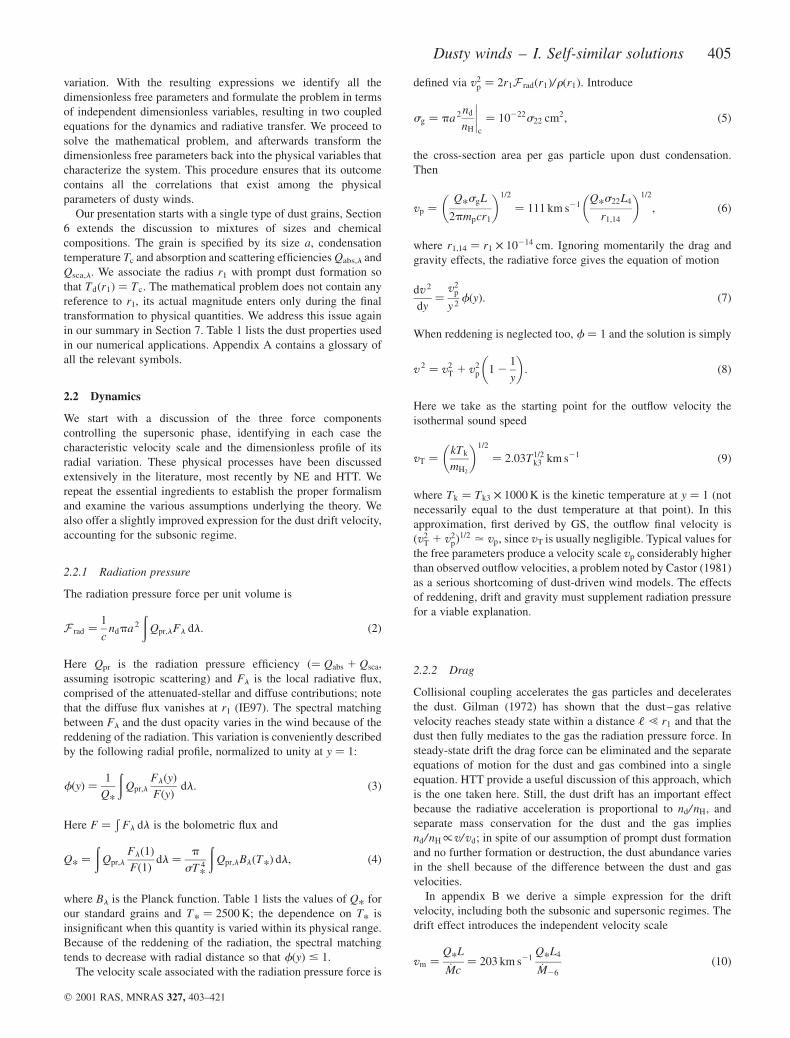
Carbon Silicate

a (mm) 0.1 0.1Tc (K) 800 800QV 2.40 1.15Q* 0.599 0.114C0 5.97 2.72

Table 1. Standard parameters for dust grains used in all numericalcalculations. The efficiency factors are from Hanner (1988) for amorphouscarbon, and Ossenkopf, Henning & Mathis (1992) for (the ‘warm’ version of)silicate grains. The grain size a and sublimation temperature Tc are assumed.The lower part lists derived quantities: QV is the efficiency factor for absorptionat visual; Q* is the Planck average at the stellar temperature of the efficiencycoefficient for radiation pressure (equation 4); C0 is defined in equation (41).

404 M. Elitzur and Z. Ivezic

q 2001 RAS, MNRAS 327, 403–421

variation. With the resulting expressions we identify all the

dimensionless free parameters and formulate the problem in terms

of independent dimensionless variables, resulting in two coupled

equations for the dynamics and radiative transfer. We proceed to

solve the mathematical problem, and afterwards transform the

dimensionless free parameters back into the physical variables that

characterize the system. This procedure ensures that its outcome

contains all the correlations that exist among the physical

parameters of dusty winds.

Our presentation starts with a single type of dust grains, Section

6 extends the discussion to mixtures of sizes and chemical

compositions. The grain is specified by its size a, condensation

temperature Tc and absorption and scattering efficiencies Qabs,l and

Qsca,l. We associate the radius r1 with prompt dust formation so

that Tdðr1Þ ¼ Tc. The mathematical problem does not contain any

reference to r1, its actual magnitude enters only during the final

transformation to physical quantities. We address this issue again

in our summary in Section 7. Table 1 lists the dust properties used

in our numerical applications. Appendix A contains a glossary of

all the relevant symbols.

2.2 Dynamics

We start with a discussion of the three force components

controlling the supersonic phase, identifying in each case the

characteristic velocity scale and the dimensionless profile of its

radial variation. These physical processes have been discussed

extensively in the literature, most recently by NE and HTT. We

repeat the essential ingredients to establish the proper formalism

and examine the various assumptions underlying the theory. We

also offer a slightly improved expression for the dust drift velocity,

accounting for the subsonic regime.

2.2.1 Radiation pressure

The radiation pressure force per unit volume is

F rad ¼1

cndpa 2

ðQpr;lFl dl: ð2Þ

Here Qpr is the radiation pressure efficiency ð¼ Qabs 1 Qsca,

assuming isotropic scattering) and Fl is the local radiative flux,

comprised of the attenuated-stellar and diffuse contributions; note

that the diffuse flux vanishes at r1 (IE97). The spectral matching

between Fl and the dust opacity varies in the wind because of the

reddening of the radiation. This variation is conveniently described

by the following radial profile, normalized to unity at y ¼ 1:

fðyÞ ¼1

Q*

ðQpr;l

FlðyÞ

FðyÞdl: ð3Þ

Here F ¼Ð

Fl dl is the bolometric flux and

Q* ¼

ðQpr;l

Flð1Þ

Fð1Þdl ¼

p

sT 4

*

ðQpr;lBlðT*Þ dl; ð4Þ

where Bl is the Planck function. Table 1 lists the values of Q* for

our standard grains and T* ¼ 2500 K; the dependence on T* is

insignificant when this quantity is varied within its physical range.

Because of the reddening of the radiation, the spectral matching

tends to decrease with radial distance so that fðyÞ # 1.

The velocity scale associated with the radiation pressure force is

defined via v2p ¼ 2r1F radðr1Þ/rðr1Þ. Introduce

sg ¼ pa 2 nd

nH

����c

¼ 10222s22 cm2; ð5Þ

the cross-section area per gas particle upon dust condensation.

Then

vp ¼Q*sgL

2pmpcr1

� �1=2

¼ 111 km s21Q*s22L4

r1;14

� �1=2

; ð6Þ

where r1;14 ¼ r1 � 10214 cm. Ignoring momentarily the drag and

gravity effects, the radiative force gives the equation of motion

dv 2

dy¼

v2p

y 2fðyÞ: ð7Þ

When reddening is neglected too, f ¼ 1 and the solution is simply

v 2 ¼ v2T 1 v2

p 1 21

y

� �: ð8Þ

Here we take as the starting point for the outflow velocity the

isothermal sound speed

vT ¼kTk

mH2

� �1=2

¼ 2:03T1=2k3 km s21 ð9Þ

where Tk ¼ Tk3 � 1000 K is the kinetic temperature at y ¼ 1 (not

necessarily equal to the dust temperature at that point). In this

approximation, first derived by GS, the outflow final velocity is

ðv2T 1 v2

pÞ1=2 . vp, since vT is usually negligible. Typical values for

the free parameters produce a velocity scale vp considerably higher

than observed outflow velocities, a problem noted by Castor (1981)

as a serious shortcoming of dust-driven wind models. The effects

of reddening, drift and gravity must supplement radiation pressure

for a viable explanation.

2.2.2 Drag

Collisional coupling accelerates the gas particles and decelerates

the dust. Gilman (1972) has shown that the dust–gas relative

velocity reaches steady state within a distance ‘ ! r1 and that the

dust then fully mediates to the gas the radiation pressure force. In

steady-state drift the drag force can be eliminated and the separate

equations of motion for the dust and gas combined into a single

equation. HTT provide a useful discussion of this approach, which

is the one taken here. Still, the dust drift has an important effect

because the radiative acceleration is proportional to nd/nH, and

separate mass conservation for the dust and the gas implies

nd/nH/v/vd; in spite of our assumption of prompt dust formation

and no further formation or destruction, the dust abundance varies

in the shell because of the difference between the dust and gas

velocities.

In appendix B we derive a simple expression for the drift

velocity, including both the subsonic and supersonic regimes. The

drift effect introduces the independent velocity scale

vm ¼Q*L

_Mc¼ 203 km s21

Q*L4

_M26

ð10Þ

Dusty winds – I. Self-similar solutions 405

q 2001 RAS, MNRAS 327, 403–421

and the steady-state drift velocity is:

vrel ¼vmvf

vT 1ffiffiffiffiffiffiffiffiffiffiffiffivmvfp ð11Þ

(equation B4). The significance of subsonic drift is rapidly

diminished with radial distance because v is increasing as the gas

accelerates while vT is decreasing as it cools down. The radial

variation of vT requires the gas temperature profile, a quantity that

does not impact any other aspect of the flow and whose calculation

contains large uncertainties. We avoid these uncertainties and use

instead the initial vT throughout the outflow. This slightly

overestimates the overall impact of subsonic drift, producing a

negligible error in an effect that is small to begin with.

The dust velocity is vd ¼ v 1 vrel, therefore nd/nH varies in

proportion to the dimensionless drift profile

zð yÞ ¼v

vd

¼vT 1

ffiffiffiffiffiffiffiffiffiffiffiffivmvfp

vT 1 vmf 1ffiffiffiffiffiffiffiffiffiffiffiffivmvfp : ð12Þ

Since pa 2ndðyÞ/ nHðyÞ ¼ sgzðyÞ for y $ 1, the force equation

including the drift effect is

dv 2

dy¼

v2p

y 2fðyÞzðyÞ: ð13Þ

Because of the drift, at y ¼ 1 the radiative force is reduced by a

factor z(1), a significant reduction when vm @ vT. The reason is

that the dust particles are produced at the velocity vT with a certain

abundance and the drift immediately dilutes that abundance within

a distance ‘ ! r1 so that nd/nH is diminished already at y ¼ 1. In

calculations that keep track separately of the dust and the gas, the

two species start with the same velocity and this dilution is

generated automatically (cf. NE, HTT). Here we solve for only one

component, the two species start with different velocities at y ¼ 1

and the initial dilution must be inserted explicitly.

It is important to note that z is a monotonically increasing

function of y (see Section 3.2 below). Therefore, the dust

abundance is the smallest at y ¼ 1 and increases from this

minimum during the outflow. At the wind outer regions, nd/ nH

exceeds its initial value by the factor zð1Þ/zð1Þ.

2.2.3 Gravity

The gravitational pull introduces an independent velocity scale, the

escape velocity at r1

vg ¼2GM

r1

� �1=2

¼ 15:2 km s21 M0

r1;14

� �1=2

; ð14Þ

which is frequently entered in terms of the dimensionless ratio

G ¼F rad

F grav

����r1

¼v2

p

v2g

¼Q*sgL

4pGMmpc¼ 45:8Q*s22

L4

M0

: ð15Þ

Gravity does not introduce any radial profile beyond its y 22

variation. Adding the gravitational effects, the equation of motion

becomes

dv 2

dy¼

v2p

y 2fðyÞzðyÞ2

1

G

� �: ð16Þ

In the limit of negligible drift and reddening ðz ¼ f ¼ 1Þ, the

gravitational pull reduces the wind terminal velocity from vp to

vpð1 2 1=GÞ1=2, typically only , 1 per cent effect.

This is the complete form of the equation of motion, including

all the dynamical processes in the wind. The outflow is fully

specified by the four independent velocity scales: vp, vm, vg and vT,

which is also the initial velocity vðy ¼ 1Þ, and the reddening profile

f. This profile varies with the overall optical depth and is

determined from an independent equation, the equation of radiative

transfer.

2.3 Radiative transfer

Because of the spherical symmetry, the radiative transfer equation

requires as input only two additional quantities (IE97). One is the

overall optical depth along a radial ray at one wavelength, which

we take as visual

tV ¼ r1sV

ðnd dy; ð17Þ

the optical depth at every other wavelength is simply tVQl/QV,

where Ql and QV are the absorption efficiencies at l and visual,

respectively. The other required input is the normalized radial

profile of the dust density distribution

hðyÞ ¼ndðyÞÐ1

1nd dy

: ð18Þ

Given these two quantities, the intensity Il(y,b ) of radiation

propagating at angle b to the radius vector at distance y can be

obtained from

dIlðy;bÞ

dtlðy;bÞ¼ Sl 2 Il; ð19Þ

where

tlðy;bÞ ¼ tV

Ql

QV

ðy cosb

0

hðffiffiffiffiffiffiffiffiffiffiffiffiffiffiffiffiffiffiffiffiffiffiffiffiffiffiffiz 2 1 y 2 sin2b

pÞ dz: ð20Þ

In general, h and tV must be specified as independent inputs.

Instead, here they are fully specified by the dynamics problem.

With the assumption of no grain growth or sputtering after its

prompt formation, mass conservation for the dust gives

nd/1/ r 2vd/z/ y 2v so that

hðyÞ ¼zðyÞ

y 2vðyÞ

ð1

1

z

y 2vdy

� �21

: ð21Þ

Therefore h is not an independent input property, instead it is

determined by the solution of the equation of motion. And

straightforward manipulations show that

tV ¼ QV

v2p

2vm

ð1

1

z

y 2vdy; ð22Þ

so tV, too, does not require the introduction of any additional

independent input. The radiative transfer problem is fully specified

by the parameters already introduced to formulate the equation of

motion; it requires no additional input.

This completes the formulation of the dusty wind problem. The

dynamics and radiative transfer problems are coupled through the

reddening profile f. The solution of the equation of motion

obtained with a certain such profile determines a dust distribution h

and an optical depth tV. The solution of the radiative transfer

equation obtained with these h and tV as input properties must

reproduce the reddening profile f that was used in the equation of

motion to derive them.

406 M. Elitzur and Z. Ivezic

q 2001 RAS, MNRAS 327, 403–421

2.4 Scaling

Given the grain properties and the spectral profile of the stellar

radiation, the wind problem is fully specified by the four

independent velocities: vp, vm, vg and vT, which together form the

complete input of the problem. Since an arbitrary velocity

magnitude can always be scaled out, the mathematical model can

be described in a dimensionless form which includes only three

parameters. We choose vm for this purpose because it results in a

particularly simple equation of motion. Introduce

w ¼ v/vm; u ¼ vT/vm; P ¼ vp/vm: ð23Þ

The parameter P characterizes the ratio of radiation pressure to

drift effects. It is very large when the drift becomes negligible and

goes to zero when the drift dominates. The equation of motion (16)

becomes

dw 2

dy¼

P 2

y 2fz 2

1

G

� �; where z ¼

u 1ffiffiffiffiffiffiffiwfp

u 1 f 1ffiffiffiffiffiffiffiwfp ð24Þ

and where f is determined from the solution of the radiative

transfer equation (19) in which the dust distribution and optical

depth are

hðyÞ ¼zðyÞ

y 2wðyÞ

ð1

1

z

y 2wdy

� �21

;

tV ¼1

2QVP 2

ð1

1

z

y 2wdy: ð25Þ

In this new form, the mathematical model is fully specified by the

three dimensionless parameters P, G and u, where the latter is also

the initial value u ¼ wðy ¼ 1Þ. The velocity must rise at the origin,

and since fð1Þ ¼ 1 the parameters are subject to the constraint

Gzð1Þ . 1; i:e: ðG 2 1Þðu 1ffiffiffiupÞ . 1: ð26Þ

This lift-off condition ensures that radiation pressure, with proper

accounting for the dust drift, can overcome the initial gravitational

pull. It can be viewed as either a lower limit on G for a given u or,

given G, a lower limit on u.

The dusty wind problem has been transformed into a set of two

general mathematical equations – the equation of motion (24) and

the radiative transfer equation (19) with the input properties from

equation (25). Given the spectral shapes of the stellar radiation and

the dust absorption coefficient, these equations are fully prescribed

by P, G and u. Both the radiative transfer and the dynamics

equations are solved without any reference to vm or any other

velocity scale. The velocity scale is an extraneous parameter,

entirely arbitrary as far as the solution is concerned. The wind

radiative emission and the shape of its velocity profile are both

independent of the actual magnitude of the velocity. In the

following discussion we show that the shape of w(y ) turns out to be

a nearly universal function, independent of input parameters within

their relevant range, and that the final velocity w1 ¼ wðy!1Þ is

for all practical purposes only a function of P.

3 S O L U T I O N S

The complete solution involves two elements – dynamics and

radiative transfer. The impact of the radiative transfer on the

dynamics can be conveniently expressed in terms of the quantity F,

defined via

w1

F¼

ðw1

u

dw

f: ð27Þ

That is, F is the velocity-weighted harmonic average of the

reddening profile f. Combining equations (24) and (25), it is easy

to show that

tV

QV

¼w1

F1

P 2

2G

ð1

1

dy

y 2wf: ð28Þ

Therefore, when gravity is negligible ðG @ 1Þ the optical depth and

the terminal velocity obey the simple relation

w1 ¼ FtV

QV

: ð29Þ

In optically thin winds F ¼ 1 and w1 ¼ tV/QV. As reddening

increases F decreases, the final velocity is affected by the radiative

transfer and numerical computations are necessary.

We obtain numerical solutions for arbitrary optical depths with

the code DUSTY (Ivezic, Nenkova & Elitzur, 1999). DUSTY

solves the dusty wind problem through a full treatment of the

radiation field, including scattering, absorption and emission by the

dust, coupled to the hydrodynamics problem formulated above.

Appendix D provides a description of the numerical procedure. We

present now the solutions, starting with the optically thin regime

where we found the exact analytic solution.

3.1 Negligible reddening

When reddening is negligible, the flux spectral shape does not vary

and f ¼ 1 (see equation 3). This is the situation in optically thin

winds, and the detailed results presented in the next section show

this to be the case when tV & 1.1 Even though the optical depth at

wavelengths shorter than the visual already exceeds unity when

tV ¼ 1 and the emerging spectrum is affected by radiative transfer,

the impact on the dynamics is minimal. The reason is that f

involves a spectral average, and the stellar radiation peaks at longer

wavelengths.

The wind problem with f ¼ 1 was called the ‘first simplified

model’ by HTT, who solved it numerically. Here we present the

complete analytic solution for this case. Since f is known, the

equation of motion decouples from the radiative transfer problem

and can be considered independently. Introduce

d ¼1

G 2 1; ð30Þ

then equation (24) can be cast in the form

1 11 1 dffiffiffiffi

wp

1 u 2 d

� �dw 2

dy¼

P 2

1 1 d

1

y 2ð31Þ

so that

w 2 2 u 2 1 4ð1 1 dÞ

ð ffiffiffiwpffiffiup

x 3 dx

x 1 u 2 d¼

P 2

1 1 d1 2

1

y

� �: ð32Þ

1 Another limit that in principle could give f ¼ 1 involves grains so large

that Ql is constant for all relevant wavelengths. This requires grain sizes in

excess of , 10mm, and seems of little relevance.

Dusty winds – I. Self-similar solutions 407

q 2001 RAS, MNRAS 327, 403–421

The lift-off constraint (26) ensures that the denominator of the

integrand never vanishes in physical solutions; it starts positive at

the lower boundary and increases as x increases. The integration is

standard, the result is

P 2

1 1 d1 2

1

y

� �¼ w 2 2 u 2 1 4ð1 1 dÞ

1

3ðw 3=2 2 u 3=2Þ

�1

1

2ðd 2 uÞðw 2 uÞ

1 ðd 2 uÞ2ðw 1=2 2 u 1=2Þ

1ðd 2 uÞ3 ln

ffiffiffiffiwp

1 u 2 dffiffiffiup

1 u 2 d

�: ð33Þ

This is the complete solution for all dusty winds with tV , 1, fully

incorporating the effects of gravity and dust drift. Radiation

reddening, which takes effect when tV . 1, is the only ingredient

missing from this analytic solution and preventing it from

applicability for all winds. The GS solution (equation 8), the only

previous analytic result, which neglected the effects of gravity and

drift in addition to reddening, can be recovered inserting d ¼ 0 and

P @ 1.

The solutions are meaningful only when describing winds in

which v1/vT is at least , 3; otherwise, the effects of gas pressure,

which were neglected here, become significant and equation

(24) loses its physical relevance. Therefore, we require

v1/vT ¼ w1/u . 3. In addition, the lift-off condition implies

that d , dmax where

dmax ¼ffiffiffiup

1 u: ð34Þ

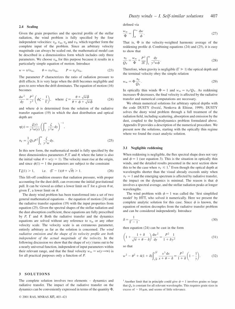
Fig. 1 displays the dimensionless velocity profile as a function of

distance y for a range of representative values of the three free

parameters and demonstrates a remarkable property. Except for

their role in determining the boundary of allowed phase space and

controlling the wind properties near that boundary, d and u hardly

matter; away from the boundary, the solution is controlled almost

exclusively by the single parameter P. Part (a) of the figure shows

Figure 1. The complete solution (equation 33) for the velocity profiles of optically thin winds. (a) In each panel P has the indicated value and the initial velocity

is u ¼ 0:03P. The solutions are plotted for various values of d, marked as fractions of the gravitational quenching value dmax. Note the virtual d-independence,

except for the solutions asymptotically close to dmax. (b) Same as (a), only now u varies and d is fixed at 0. The values of u are listed as fractions of umax, the

initial velocity that yields the smallest meaningful velocity increase w1/u ¼ v1/vT ¼ 3. Note the complete u-independence, except for the solution with

u ¼ umax.

408 M. Elitzur and Z. Ivezic

q 2001 RAS, MNRAS 327, 403–421

the effect of varying d when P and u are held fixed. Each panel

presents a representative value of P with a wind initial velocity

u ¼ 0:03P; this choice of u ensures that the wind velocity increases

by a factor of , 10–20 in each case. The displayed values of d

cover the entire physical range for this parameter, from 0 to just

below the singularity at dmax. In each panel, the solutions for

d/dmax # 1=2 are similar to each other, those with d/dmax # 1=4

hardly distinguishable. All display a similar rapid rise within y &

10 towards a final, nearly the same velocity. The plots for d/dmax $

0:999 stand out and show the quenching effect of gravity, which is

discussed below (Section 5.1).

The effect of u on the solution when d and P are held fixed are

similarly shown in part (b) of the figure. In these panels d ¼ 0. This

value was chosen because it represents faithfully most non-

quenched solutions while allowing the wind to start with arbitrarily

small initial velocity, even zero. The values of u for the displayed

solutions are listed as fractions of umax, the initial velocity that

leads to w1/u ¼ 3 for the listed P. As is evident from the plots, the

initial velocity is largely irrelevant. Starting from u ¼ 0 or as much

as 1/2umax yields practically the same results. The only discernible

difference occurs at umax, where the profile deviates from the

common shape by no more than , 10 per cent.

The analytic solution defines w as an implicit function of y. In

appendix C we derive explicit analytic expressions for w that

provide adequate approximations in all regions of interest. An

inspection of the solution shows that P ¼ 16=9 is the transition

between the drift-dominated regime at small P and negligible drift

at large P. The velocity profiles in the two are:

w ¼ w1 1 21

y

� �k

; k ¼2=3 for P , 16=9

1=2 for P . 16=9

(: ð35Þ

The expressions for w1 in the two regimes can be combined into

the single form

w1 ¼ PP

P 1 169

!1=3

: ð36Þ

The optical depth, needed for the radiative transfer problem which

is solved independently in this case, is simply tV ¼ QVw1 (see

equation 29). Appendix C provides the d and u corrections to these

results, which show that the dependence on u is confined to the very

origin of the wind, y 2 1 & u/w1.

The last two expressions reproduce to within 30 per cent the

plots for all the non-quenched winds displayed in Fig. 1. They

amplify our conclusion about the negligible role of both d and u

away from the physical boundary and point to another remarkable

property of the solution. Although the final velocity strongly

depends on P, the shape of the velocity profile w/w1 does not. The

only reference to P in this profile is in determining a transition to a

slightly steeper profile shape at large P. The profile itself is

independent of P in either regime and furthermore, the difference

between the two shapes is not that large. These properties are

evident from Fig. 1. Other than the numerical values on the vertical

axis, it is hard to tell apart the plots in the different panels.

These results show that among the three independent input

parameters, P is the only one to have a significant effect on any

property of interest. Furthermore, even P affects mostly just the

final velocity, it does not have a discernible effect on the shape of

the velocity profile; all optically thin winds share universal

velocity and dust density profiles.

3.2 Reddening effects

The results for optically thin winds carry over to arbitrary optical

depths, with profound implications for all winds. Reddening

effects are controlled by the wind optical depth and density profile.

For a given pair of d and u, consider a value of P sufficiently small

that tV ! 1 so that reddening can be neglected; such a choice of P

is virtually always possible. The velocity profile and tV are then

uniquely determined by P (equations 35 and 36) and so is the

radiative transfer problem. When P increases, tV increases too. The

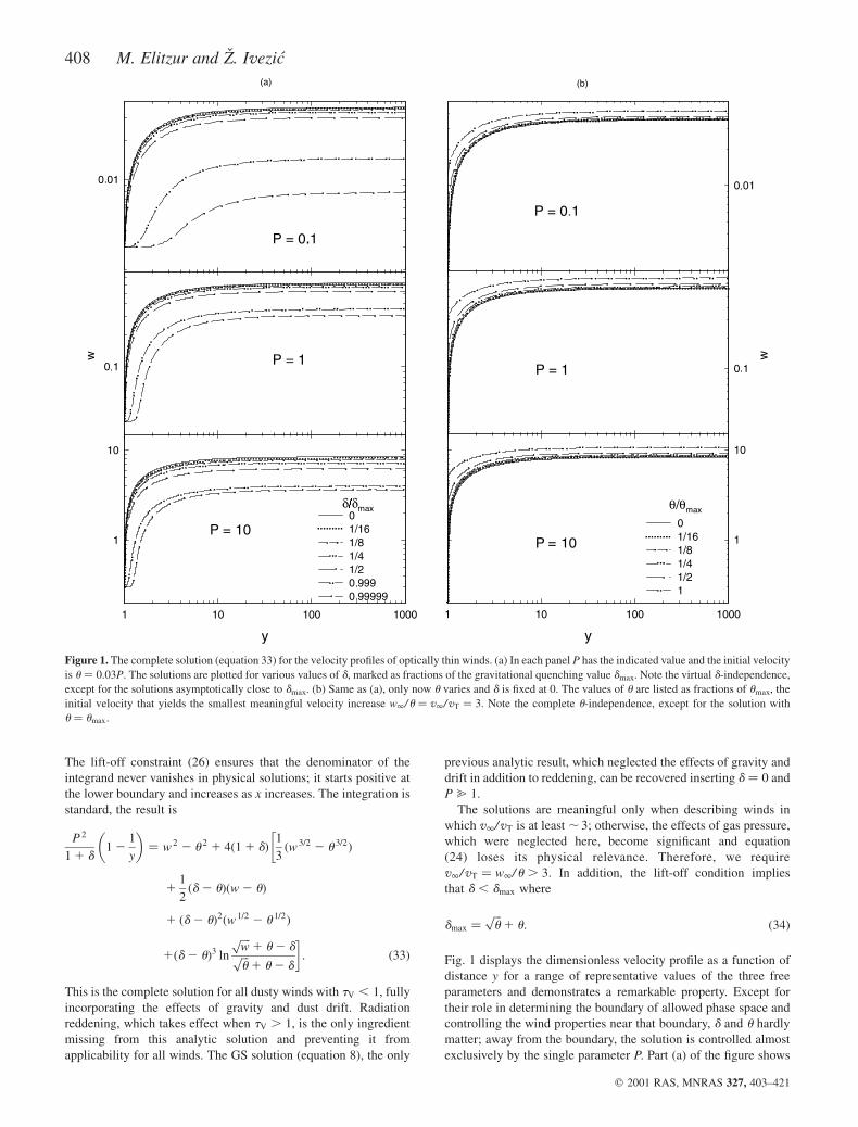
Figure 2. Radial profiles for quantities of interest at various values of P, as

marked. The corresponding optical depths are shown in parenthesis. All

models have amorphous carbon grains, d ¼ 0 and w1/u ¼ 10.

Dusty winds – I. Self-similar solutions 409

q 2001 RAS, MNRAS 327, 403–421

results of appendix C show that

P ¼1

QV

1 14

3Q1=2

V

� �1=2

ð37Þ

yields tV ¼ 1; with our standard grains, the corresponding values

are P ¼ 0:73 for carbon and P ¼ 1:35 for silicates. As P increases

further the optical depth increases too and with it the impact of

reddening, and that impact too is controlled exclusively by P.

Therefore, the parameter P controls all aspects of the problem. As

concluded in IE95, away from its boundary and for most of the

phase space the dusty wind problem is controlled by a single free

parameter. Since P, tV and w1 are uniquely related to each other,

either one can serve as that free parameter.

Fig. 2 shows the radial variation of profiles of interest for various

values of P. The models for P ¼ 0:1, 1 and 10 repeat those

presented in Fig. 1 but fully incorporate radiative transfer.

Comparison of the corresponding plots in the two figures illustrates

the impact of reddening. The bottom panel of Fig. 2 shows the

reddening profile f. Most of the reddening occurs close to the wind

origin. Reddening becomes significant at P ¼ 1, and substantial at

P ¼ 10 and 100. Still it has only a minimal impact on the velocity

profile; as is evident from the top panel, the dependence of the

profile shape on P remains weak. We find that equation (35)

remains an excellent approximation under all circumstances, the

effect of reddening merely decreases the exponent k from 0.5 to 0.4

at large P. The plots of z show that most of the drift variation, too,

occurs close to the origin. At y * 2 the dust and gas velocities

maintain a constant ratio, which can be substantial when P is small;

at P ¼ 0:1 the final velocity of the dust grains exceeds that of the

gas particles by more than a factor of 6. The velocity and drift

profiles combine to determine the dust density profile h (see

equation 25). The figure presents the function y 2h, removing the

common radial divergence factor 1/ y 2.

The plots present the full solutions of the dynamics problem

coupled with radiative transfer for carbon grains. The results for

silicate grains are essentially the same, extending the conclusion

reached in the optically thin limit to all cases: all radiatively driven

dusty winds share nearly identical velocity and dust density

profiles.

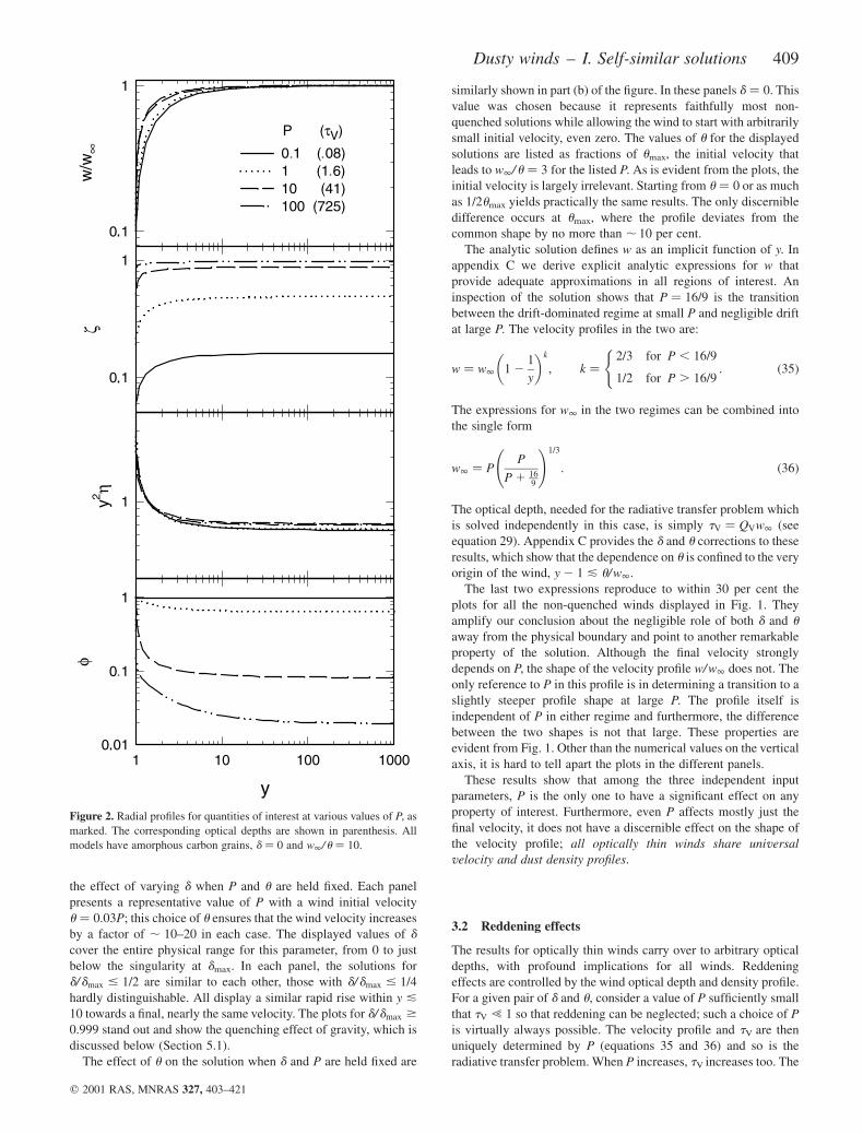
Fig. 3 presents the dependence of tV/QV ð¼ w1/FÞ and final

velocity w1 on P. The bottom panel shows the reddening indicator

F. As long as F ¼ 1, reddening is negligible, the analytic solution

(33) holds and the grain properties are irrelevant. Indeed, all

quantities are the same for carbon and silicate dust in that regime.

The grain composition matters only when reddening affects the

dynamics. The figure shows that F begins to decrease, indicating

that reddening becomes significant, at a value of P corresponding

to tV . 1; the actual value is controlled by QV (equation 37), it is

larger for silicate because of its smaller QV. As noted before, the

optical depth at wavelengths shorter than the visual already

exceeds unity when tV ¼ 1, but that spectral region has little

impact on the dynamics.

Appendix B shows that the analytic approximation in equation

(36) can be extended to include reddening effects,

w1 ¼ PffiffiffiffiFp P

P 1 169

ffiffiffiffiFp

!1=3

: ð38Þ

This expression provides an excellent approximation for the

numerical results presented in Fig. 3; the deviations are less than 10

per cent for silicate grains, 30 per cent for carbon. In addition to

w1, the figure displays also w1/P ¼ v1/vp. As discussed in

Section 2, the simplest application of radiation pressure gives the

GS result v1 ¼ vp, i.e. w1/P ¼ 1. The figure shows that the actual

solution has a substantially different behaviour – w1/P is neither

constant, nor does it reach unity. Instead, it increases in proportion

to P 1/3 at P & 1, because of the drift, and decreases in proportion

to F1/2 at P * 1, because of the reddening. Its maximum, reached

around P , 1, is larger for silicate because it requires larger P for

reddening to become significant. Drift and reddening play a crucial

role in the behaviour of w1/P. The maximum reached by this

function translates to a maximum velocity for dusty winds,

discussed in the next section.

Figure 3. Variation with P of various quantities of interest.

410 M. Elitzur and Z. Ivezic

q 2001 RAS, MNRAS 327, 403–421

4 O B S E RVA B L E C O R R E L AT O N S

Contact with observations is made by transforming the

mathematical problem back into physical quantities. Except for

regions close to the boundary of phase space (see Section 5), the

wind problem is fully controlled by the parameter P and its solution

determines the corresponding w1. Both quantities will now be

expressed in terms of physical parameters.

The main scaling variable is

P ¼ 0:546 _M26

s22

Q*L4r1;14

!1=2

ð39Þ

(see equation 23). This expression does not determine P explicitly

because P enters indirectly also on its right-hand side. The dust

condensation condition Tðr1Þ ¼ Tc determines r1 as (IE97):

r1 ¼LC

16psT4c

� �1=2

¼ 1:16 � 1014 L1=24 C1=2

T2c3

cm: ð40Þ

Here Tc3 ¼ Tc/ ð1000 KÞ and C is a dimensionless function

determined by the radiative transfer, similar to the reddening

profile, and thus dependent on P. Optically thin winds have C ¼

C0 where

C0 ¼QPðT*Þ

QPðTcÞ: ð41Þ

Here QP(T ) is the Planck average of the absorption efficiency,

similar to the average of the radiation pressure efficiency that

defines Q* (equation 4); Table 1 lists C0 for our standard

grains. As P increases, the wind becomes optically thick and C

increases too. In IE97 we present the variation of C=C0 with

optical depth and show that it is well approximated by the

analytic expression

C

C0

¼ 1 1 3tV

QV

QPðTcÞ �f ð42Þ

where

�f ¼

ðfðyÞhðyÞ

dy

y 2

(see fig. 1 and equation B7 in IE97).2 Just as F is the velocity-

weighted harmonic average of the reddening profile, f is its

standard average, weighted by h/ y 2.

For most of the relevant region of phase space, P fully controls

the solution of the dusty wind problem. Since C is part of that

solution, it too depends only on P. Therefore, the combination of

equations (39) and (40) results in

_M26

L3=44

¼ 1:98Q1=2

*s1=2

22 Tc3

PC1=4; ð43Þ

a one-to-one correspondence between _M/L 3=4 and P. This

correspondence involves the function PC1/4, which is fully

determined from the solution of the mathematical wind problem.

The proportionality constant involves the individual grain

properties Q* and Tc which are part of the problem specification,

and s22 which is not. The dust abundance, necessary for specifying

s22, has no effect on the wind solution; only the proportionality

constant is modified when this abundance is varied, the function

PC1/4 remains the same.

This result shows that for any dusty wind, the combination_M/L 3=4 can be determined directly from the shape of the spectral

energy distribution: the wind IR signature is fully controlled by the

parameter P, therefore comparing the observations with a bank of

solutions determines the value of P and equation (43) fixes _M/L 3=4.

We may expect all C-rich stars to have dust with roughly similar

abundance and individual grain properties, so that they have the

same proportionality constant and functional dependence C(P );

likewise for O-rich stars. In that case, each family defines a unique

correspondence between _M/L 3=4 and P. And since the parameter P

fully controls the IR signature, stars that have different M and L but

the same _M/L 3=4 are indistinguishable by their IR emission because

they also have the same P.

The solution of the wind problem also determines w1, another

unique function of P. Therefore, the relation v1/vm ¼ w1 gives

another one-to-one correspondence between P and an independent

combination of physical quantities

_Mv1

L¼

1

cQ*w1: ð44Þ

Since this correspondence does not involve s22, it is independent of

the dust abundance and depends only on individual grain

properties. Systems with different M, Landv1 but the same_M/L 3=4 necessarily have also the same _Mv1/L because each

combination uniquely determines the parameter P of the system.

The complete description of the wind problem involves four

velocity scales, two of which (vT and vg) do not count whenever G

and u can be ignored. For most of the phase space the problem is

fully specified by the velocities vp and vm, and its solution

determines v1. The two ratios formed out of these three velocities

are all the independent dimensionless combinations of physical

parameters to determine the mathematical wind model and its

solution. Since this solution fully specifies the wind IR signature,_M/L 3=4 and _Mv1/L are the only combinations of global parameters

that can be determined from IR observations, even the most

detailed ones. When the velocity is additionally measured in

molecular line observations, so that both P and v1 are known, the

two combinations in equations (43) and (44) can be used to

determine also L and M individually. The relevant correlations

are:

v1

L 1=4/

w1

PC1=4;

v31

_M/

w31

P 4C; ð45Þ

whose constants of proportionality can be trivially derived. Only

two of the last four combinations that relate M, L and v1 to the

solution are independent; any two of them can be derived from the

other two.

4.1 Similarity relations

While P is the natural independent variable of the mathematical

problem, its physical interpretation is only indirect. Modelling of

IR observations directly determines tV, not P. Therefore, we now

express all results in terms of tV by performing a straightforward

change of variables. The relation between tV and P is non-linear,

2 Since scattering is neglected in the IE97 analytic solution, the difference

between Q* and QP(T*) is ignored in the approximations here (but not in the

numerical calculations).

Dusty winds – I. Self-similar solutions 411

q 2001 RAS, MNRAS 327, 403–421

starting from P/t3=4V in the optically thin regime and switching to

a more complex dependence when reddening becomes significant.

We introduce the tV–P transformation function Q through

P ¼2ffiffiffi3p

tV

QV

� �3=4

Q ð46Þ

so that Q ¼ 1 when tV , 1. At larger optical depths, Q can only be

determined from the numerical solution. The analytic expression

Q2 . 1 1

3

4ðtV/QVÞ

1=2

� �F; ð47Þ

obtained from equation (C12), provides a useful approximation

for the numerical results at all optical depths. With the tV–P

transformation, equation (43) becomes

_M26

L3=44

¼ c1t3=4V K1ðtVÞ; ð48Þ

where

K1 ¼C

C0

� �1=4

Q; c1 ¼ 2:28Q1=2

* C1=40

Q3=4V s1=2

22 Tc3

:

From its definition K1 ¼ 1 when tV , 1, therefore _M26 ¼

c1ðL4tVÞ3=4 in all optically thin winds. As the optical depth

increases, K1 introduces the reddening correction to this relation.

This correction, purely a function of tV, is shown in the top panel of

Fig. 4.

The transformation of the other independent correlation from P

to tV is considerably simpler. Thanks to equation (29), which holds

for all winds when gravity is negligible, equation (44) can be cast

similarly in the form

_Mv1

L¼

1

cðQ*/QVÞtVK2ðtVÞ; ð49Þ

where K2 ¼ F. The function K2, shown in the second panel of Fig.

4, contains the reddening corrections to the optically thin

correlation, similar to the previous result. Since K2 ¼ F, it is the

same function as shown in Fig. 3, only plotted against the

independent variable tV instead of P.

This completes the transformation from P to tV of the two

independent correlations. In both, the luminosity does not enter

independently, only through the product LtV. In the case of

equation (49) this is a direct consequence of the structure of the

equation of motion, which gives v1 ¼ vmw1 ¼ vmtVðF/QVÞ. The

combination LtV emerges here as a ‘kinematic’ result irrespective

of the explicit expression for the drift function. In the case of

equation (48), on the other hand, this combination is a direct

consequence of the specific functional form of z. With these two

results, the correlations in equation (45) become similarly

v1

L1=44

¼ c3t1=4V K3ðtVÞ;

v31

_M26

¼ c4K4ðtVÞ ð50Þ

where K3 ¼ K2/K1 and K4 ¼ K32/K4

1. The associated proportion-

ality constants are:

c3 ¼ 88:9Tc3ðQ*s22Þ1=2ðQVC0Þ

21=4;

c4 ¼ 3:08 � 105T4c3Q*s

222C

210 : ð51Þ

Since L enters only in the form LtV, the combination that eliminates

L eliminates also tV from its optically thin regime. The reddening

correction functions K3 and K4 are shown in the two bottom panels

of Fig. 4.

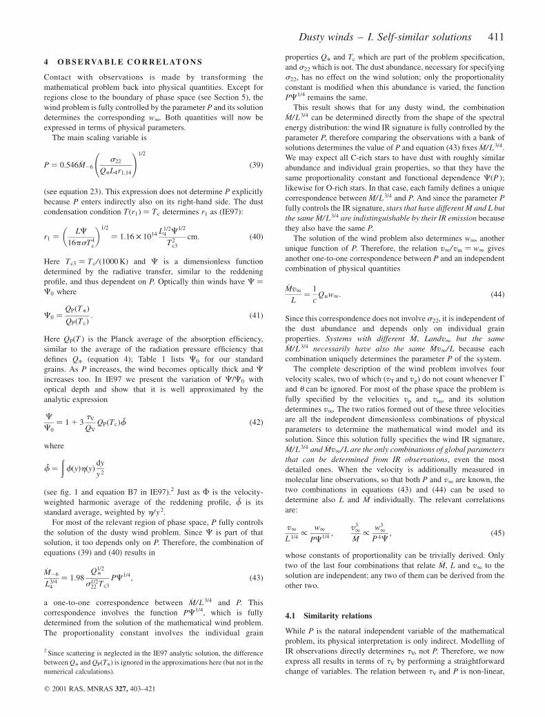
At small tV the grain properties are irrelevant and the similarity

K-functions are unity for both silicate and carbon dust. As tV

increases the curves for the two species diverge, reflecting their

different optical properties. However, Fig. 4 shows that the

differences are moderate in all four cases. They are most noticeable

in K1 and K2, where the relative differences from the mean never

Figure 4. The reddening corrections in the scaling relations that summarize

the physical contents of the solution (equations 48–50). Note the linear

scale in the plot of K1. The full and dashed lines show the results of detailed

numerical calculations for carbon and silicate grains, respectively. The

dotted line in the panel for Ki ði ¼ 1…4Þ plots the function 1=ð1 1 tVÞai

where a1 ¼ 20:105, a2 ¼ 0:36, a3 ¼ 0:465 and a4 ¼ 1:5.

412 M. Elitzur and Z. Ivezic

q 2001 RAS, MNRAS 327, 403–421

exceed , 25 per cent. It is also important to note that the displayed

range of tV greatly exceeds the observed range since cases of

tV * 10 are rare. The differences are greatly reduced in the ratio

function K3 ð¼ K2/K1Þ and practically disappear in K4. This

function is essentially the same (within a few per cent) for both

silicate and carbon grains at all optical depths, an agreement

maintained over many orders of magnitude. Evidently, K4 is

independent of chemical composition.

The universality of K4 is no accident. From the analytic

approximations for C (equation 42) and Q (equation 47), at large

optical depths, t2VK4/F/ �f; i.e., apart from the explicit

dependence on tV, the variation of K4 comes from the ratio of

two averages of the reddening profile, one (F) strongly weighted

towards the outer part of the shell and the other (f ) towards the

inner part. Although F and f are different for grains with different

optical properties, their ratio is controlled by the shapes of the

density and velocity profiles – which are universal, as shown

above. As a result, the functional dependence of K4 on tV is the

same for all grains when tV @ 1 in addition to tV , 1. This does

not yet guarantee a universal profile because the transition between

the two regimes could depend on the grain parameters. Indeed, the

plot of F ð¼ K2Þ shows that the large-tV decline of this function is

delayed for silicate in comparison with carbon dust. As explained

in the discussion of Fig. 3, the onset of reddening requires a larger

tV for silicate because of its smaller QV. However, the behaviour of

the factor 1 1 34ðtV/QVÞ

1=2 in Q (equation 47) is precisely the

opposite since its large-tV behaviour starts earlier when QV is

smaller. The two effects offset each other, producing a universal

shape.

The simple analytic expression ð1 1 tVÞ21:5 fits the function K4

to within 20 per cent over a variation range covering more than four

orders of magnitude, providing the nearly perfect fit evident in

Fig. 4. Therefore, dusty winds obey the condition

v31

_M26

ð1 1 tVÞ1:5 ¼ c4: ð52Þ

This result provides a complete separation of the system global

parameters from the grain parameters. The combination of v1, M

and tV on the left-hand side is always constant, its magnitude is

determined purely by the dust properties. This expression makes it

evident again that the optically thin regime corresponds to tV , 1.

As is evident from Fig. 4, K3 too is nearly the same for carbon

and silicate grains. The reason is that K3 ¼ ðK2K4Þ1=4 and the only

difference between the two species comes from their K2 profiles,

which enter only in the fourth root. The single analytic expression

ð1 1 tVÞ20:465 provides an excellent fit for both silicate and carbon

grains, leading to the independent correlation

v1 ¼ c3ðL4tVÞ1=4ð1 1 tVÞ

20:465: ð53Þ

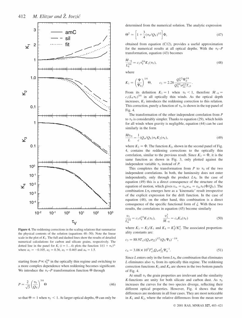
This result can explain the narrow range of velocities observed in

dusty winds. The dependence of velocity on tV at fixed luminosity

and grain properties is shown in Fig. 5. This function reaches a

maximum of 0.73 at tV ¼ 1:3, therefore the largest velocity a dusty

wind can have is

vmax ¼ 0:73c3L1=44 km s21: ð54Þ

Fig. 5 shows that the deviations from this maximum are no more

than a factor of , 2 when tV is varied in either direction by two

orders of magnitude. The dependence of velocity on luminosity is

only L 1/4, and since L4 is typically , 0:3–20 it introduces a

similarly small variation. Finally, even the dependence on grain

properties is weak, as is evident from the expression for c3

(equation 51). The only grain parameter that enters linearly is the

condensation temperature, and its dispersion is expected to be

small.

Since only two of the K-functions are independent, the universal

fits for K3 and K4 can be used to produce grain-independent

approximations also for K1 and K2. Fig. 4 shows that the single

function K33/K4 ¼ ð1 1 tVÞ

0:105 provides an adequate fit for K1 of

both silicate and carbon dust, always within 30 per cent of the

detailed results.3 This expression gives

_M26 ¼ c1ðL4tVÞ3=4ð1 1 tVÞ

0:105: ð55Þ

Since tV ¼ 1:3 gives the largest possible velocity at a given L, the

corresponding mass-loss rate is

_M26ðvmaxÞ ¼ 1:33c1L3=44 : ð56Þ

A common practice in the analysis of observations is to deduce the

optical depth from spectral data and derive M from tV (e.g. Jura

1991). This procedure is predicated on the assumption of a linear

relationship between M and tV, and our result shows that this

assumption is not right. At a fixed luminosity, M is proportional to

t3=4V in the optically thin regime and to t0:86

V at large tV. The

expectation of a linear relationship between M and tV is not met

because of the dust drift, since tV/ _M/Ððz/ y 2vÞ dy. The

relationship would be linear if z were 1 everywhere, but Fig. 2

shows that this is never the case. The deviations from unity are

large at small tV, where the drift is most prominent, decreasing as

tV increases.

Finally, Fig. 4 shows that the universal profile K43/K4 ¼

ð1 1 tVÞ20:36 again describes reasonably the actual K2 of both

grains, so that

_Mv1 ¼L

cðQ*/QVÞtVð1 1 tVÞ

20:36: ð57Þ

The relation _Mv1 # L/c has often been used as a physical bound

on radiatively driven winds, even though the mistake in this

Figure 5. The tV variation of the correlations given by equations (53) and

(57).

3 Higher accuracy, when desired, can be obtained by replacing the common

index 0.105 with 0.05 for amorphous carbon and 0.15 for silicate grains.

Dusty winds – I. Self-similar solutions 413

q 2001 RAS, MNRAS 327, 403–421

application when tV . 1 has been pointed out repeatedly. In IE95

we show that the proper form of momentum conservation is_Mv1 ¼ tFL/c where tF is the flux-averaged optical depth, so now

we have found the explicit expression

tF ¼ ðQ*/QVÞtVð1 1 tVÞ20:36: ð58Þ

The tV variation of this function is shown in Fig. 5. It increases

linearly at small tV, reaches unity at tV ¼ 1:6 and switches to t0:64V

thereafter. The ratio Q*/QV is 0.1 for silicate and 0.25 for carbon

(see Table 1).

For every pair among M, L and v1, equations (52), (53) and (55)

list the correlation in terms of optical depth. When detailed IR data

are not available and tV cannot be determined, it can be bypassed

by correlating the pairs directly against each other. Since only two

of the three relations are independent, there is only one such

combination. Equation (55) is the most suitable for eliminating tV

because K1 varies the least among the four K-functions. In fact, the

crude approximation K1 . 1 introduces an error of less than 50 per

cent for tV & 10. With this approximation, tV/ _M 4=3/L. Inserting

this result in equation (52) yields

v31 ¼ A _M26 1 1 B

_M4=3

26

L4

!21:5

ð59Þ

where A ¼ c4 and B ¼ c24=31 . This universal correlation summar-

izes our solution for all dusty winds away from the boundaries of

phase space. The error in this result, introduced by the

approximation K1 ¼ 1, is less than 50 per cent when tV # 10.

When the observational accuracy warrants higher precision,

corrections can be readily derived.

This completes the similarity solution of the dusty wind

problem. Our results amplify the conclusion of IE95, taking it a

step further: the solution is fully characterized by optical depth.

The relations among global parameters M, L and v1 involve

universal similarity functions of tV, independent of chemical

composition. The grain properties enter only in the proportionality

constants of the similarity relations. We derived the similarity

functions from solutions for carbon and silicate grains, whose

absorption efficiencies are widely different. Since dust spectral

features have a negligible effect on overall reddening corrections,

these functions should describe all interstellar grains with

reasonable properties. It is gratifying that in spite of its great

complexity, the dusty wind problem can afford such a simple,

explicit solution.

4.2 Young’s correlation

Young (1995) conducted a survey of nearby Mira variables with

low mass-loss rates. He finds a clear, strong correlation between

outflow velocity and mass-loss rate, but independent of luminosity.

The correlation can be parametrized as _M/va1, with a ¼ 3:35.

Subsequent observations by Knapp et al (1998) corroborate

Young’s results and find a ¼ 2, although the scatter in their data is

consistent with values as large as 3. Remarkably, even though the

wind is driven by radiation pressure, its velocity is independent of

luminosity.

From equation (52) or (59), at small optical depths our solution

gives _M/v31 independent of luminosity, explaining the observa-

tional findings. The implied a ¼ 3 is consistent with all

observational results within their errors. This result reflects the

central role of drift at small mass-loss rates. When the drift

dominates, z . w 1=2/ð _Mv/LÞ1=2. Neglecting gravity and reverting

to physical variables, the equation of motion (13) becomes

dv 2

dr/ð _MLvÞ1=2

r 2ð60Þ

where the proportionality constant contains the grain properties.

The solution gives v3=21 /ð

_MLÞ1=2/ r1. And since r1 is proportional to

L 1/2 (equation 40), the dependence on luminosity cancels out. If

not for the particular L dependences of r1 and the drift, this would

not have happened.

The observed correlation, in particular its luminosity indepen-

dence, directly reflects the specific dependence of the drag force on

M, L and v. Other forms for the force would produce different

correlations. For example, when the drift is neglected, the

combination (MLv )1/2 is replaced by L, leading to the GS result

v1 ¼ vp/ðL/r1Þ1=2 (equation 6). Together with r1/L 1=2 this

yields v41/L, as first noted by Jura (1984). This prediction of a

correlation between velocity and luminosity independent of mass-

loss rate is in strong conflict with the observations. One could

formally eliminate the luminosity with the aid of the momentum

flux conservation _Mv1 ¼ tFL/c (see equation 57 and subsequent

discussion) to rewrite this result as _M/tFv31. While this bears

superficial resemblance to Young’s correlation, the observational

result emerges only if the variation of tF with L and M is ignored.

In contrast, at tV , 1 equations (55) and (58) together give

tF/tV/ _M 4=3/L.

Young’s correlation is a direct reflection of the basic physics

ingredients that went into the model. It demonstrates the

importance of drift in dusty winds and provides strong support

for its underlying theory.

5 P H Y S I C A L D O M A I N

A global property not considered thus far is the stellar mass. This

quantity does not enter into the definition of the parameter P and

thus cannot be determined in general. The mass only affects G (see

equation 15), a quantity that can vary by orders of magnitude

without a discernible effect on any observed property. However, G

does play an important role in determining the parameter range

corresponding to actual winds.

The equation of motion (24) has many mathematical solutions

but not all of them are physically relevant. For example, consider

the analytic solution for optically thin winds (equation 33), whose

logarithmic term becomes singular when d ¼ dmax (see equation

34). The singularity is avoided whenever the numerator and

denominator are finite and have the same sign. Both cases are

mathematically acceptable but the negative sign is physically

meaningless. Such solutions violate the lift-off condition (equation

26) and the only transition from one set of solutions to the other is

through the singularity.

At the outset, P, G and u must be positive. Further, all winds must

obey the lift-off condition, which involves only two out of the three

input parameters. This condition ensures lift-off under all

circumstances but it does not automatically guarantee a meaningful

outcome. The formal solution of equation (24) gives

w21 ¼ u 2 1 P 2

ð1

1

fzdy

y 22

1

G

� �: ð61Þ

Obviously, in physical solutions the final velocity must exceed the

initial velocity and we further require v1/vT * 3 (see Section 3.1).

414 M. Elitzur and Z. Ivezic

q 2001 RAS, MNRAS 327, 403–421

Because f # 1 and z , 1,Ð1

1ðfz/ y 2Þ dy , 1 and

P 2 . u 2 G

G 2 1

v21

v2T

2 1

� �: ð62Þ

The three parameters of every dusty wind whose velocity increases

by the ratio v1/vT must also obey this constraint.

5.1 Gravitational quenching

The wind acceleration is positive as long as Gfz . 1 (equation 24).

Negative acceleration, leading to wind quenching, can be caused

by increasing either the gravitational pull (smaller G) or the

reddening (smaller f ). The quenching process depends on all three

input parameters and takes different forms in the optically thick

and thin regimes. In optically thin winds f ¼ 1 and since z

increases monotonically with w (cf. Fig. 2), the lift-off condition

ensures positive acceleration everywhere. Consider the analytic

solution (equation 33) when d increases while P and u remain

fixed. When b ¼ d/dmax approaches unity the acceleration

becomes negligible, although it remains positive, producing the

behaviour seen in the plots for b ¼ 0:999 and 0.99999 in Fig. 1.

This quenching effect is caused by the logarithmic term. Near

y ¼ 1 this term dominates and the velocity increases very slowly.

At a distance y roughly proportional to P 22u 3=2|lnð1 2 bÞ|, the

terms independent of d take over and the acceleration picks up.

From that point on the solution resembles non-quenched winds,

albeit at a lower acceleration because of its late start. As b gets

closer to unity, the dominance of the logarithmic term is slowly

extended further out until the whole wind is stalled.

Reddening introduces an entirely different quenching mode,

affecting winds that obey the lift-off condition when P is increased

beyond a certain point. The lift-off condition ensures that the initial

acceleration is always positive, irrespective of optical depth.

However, subsequent reddening can reduce f substantially (Fig. 2)

and since the acceleration is proportional to fz 2 1=G, the wind

may be prevented from reaching a significant terminal velocity.

Furthermore, since fz , f the acceleration becomes negative

whenever f , 1=G and the velocity can even decline after its initial

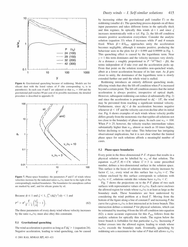
rise. Fig. 6 shows examples of such winds whose velocity profile

differs greatly from the monotonic rise that typifies all solutions not

too close to the boundary of phase space. In each case w1 ¼ 10u.

When P * 25, however, the velocity reaches intermediate values

substantially higher than w1, almost as much as 10 times higher,

before declining to its final value. This behaviour has intriguing

observational implications, but it is not clear whether the limited

phase space for such solutions affords a meaningful number of

cases.

5.2 Phase-space boundaries

Every point in the three-dimensional P–G–u space that results in a

physical solution can be labelled by w1 of that solution. The

equation w1ðP;G; uÞ ¼ Cu, where C $ 3 is some prescribed

number, defines a two-dimensional surface in the solution space.

This surface is the locus of solutions whose velocity increases by

factor C, i.e., every wind on this surface has v1/vT ¼ C. The

volume enclosed by this surface corresponds to solutions with

v1/vT $ C, solutions outside this volume have v1/vT , C.

Fig. 7 shows the projections on to the P–G plane of two such

surfaces with representative values of v1/vT. Each curve encloses

the allowed region for winds whose v1/vT is at least as large as the

boundary mark. These boundaries are best understood by

considering the wind problem at a fixed G. Moving from the

bottom of the figure along a line of constant G and increasing P, the

curve for a given v1/vT is first intersected at its lower branch. This

intersection defines a minimal P for physical solutions, which can

be estimated by inserting u from the lift-off condition into equation

(62); a more accurate expression for this Pmin follows from the

analytic solution for optically thin winds. The region below the

lower branch is forbidden for that particular v1/vT. Increasing P

further crosses into the allowed region, leading to winds whose

v1/vT exceeds the boundary mark. Eventually, quenching by

reddening sets a maximum to the value of P that still allows v1/vT

Figure 6. Gravitational quenching because of reddening. Models are for

silicate dust with the listed values of P (the corresponding tV is in

parenthesis). In each case u and G are adjusted so that w1 ¼ 10u and the

gravitational pull reaches 99 per cent of its possible maximum; the detailed

procedure is described in appendix D.

Figure 7. Phase-space boundary: the parameters P and G of winds whose

velocities increase by the indicated ratios v1/vT must lie to the right of the

correspondingly marked boundaries. The boundaries for amorphous carbon

are marked by amC, and for silicate grains by sil.

Dusty winds – I. Self-similar solutions 415

q 2001 RAS, MNRAS 327, 403–421

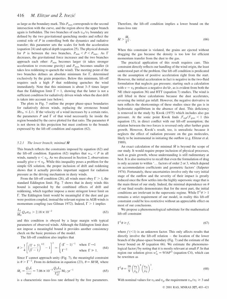
as large as the boundary mark. This Pmax corresponds to the second

intersection with the curve, and the region above the upper branch

again is forbidden. The two branches of each v1/vT boundary are

defined by the two gravitational quenching modes and reflect the

central role of P in controlling both the dynamics and radiative

transfer; this parameter sets the scales for both the acceleration

(equation 24) and optical depth (equation 25). The physical domain

for P is between the two branches, Pmin , P , Pmax. As G

decreases, the gravitational force increases and the two branches

approach each other: Pmin becomes larger (it takes stronger

acceleration to overcome gravity) and Pmax becomes smaller (it

takes less reddening to quench the wind). The meeting point of the

two branches defines an absolute minimum for G, determined

exclusively by the grain properties. Below this minimum, lift-off

requires such a high P that reddening quenches the wind

immediately. Note that this minimum is about 3–5 times larger

than the Eddington limit G ¼ 1, showing that the latter is not a

sufficient condition for radiatively driven winds when the dust drift

is taken into account (see below).

The plots in Fig. 7 outline the proper phase-space boundaries

for radiatively driven winds, replacing the erroneous bound_Mv1 # L /c. If the velocity of a wind increases by a certain ratio,

the parameters P and G of that wind necessarily lie inside the

region bounded by the curve plotted for that ratio. The parameter u

is not shown in this projection but must conform to the bounds

expressed by the lift-off condition and equation (62).

5.2.1 The lower branch; minimal M

This branch reflects the constraints imposed by equation (62) and

the lift-off condition. Equation (62) implies that w1 , P in all

winds, namely v , vp. As we discussed in Section 2, observations

usually give v ! vp. While this inequality poses a problem for the

simple GS solution, the proper inclusion of drift and reddening

shows that it actually provides important support for radiation

pressure as the driving mechanism in dusty winds.

From the lift-off condition (26), all winds must obey G . 1, the

standard Eddington limit. Fig. 7 shows that in dusty winds this

bound is superseded by the combined effects of drift and

reddening, which together impose a more stringent lower limit on

G. The Eddington limit would be meaningful if the dust and gas

were position coupled, instead the relevant regime in AGB winds is

momentum coupling (see Gilman 1972). Indeed, G . 1 implies

L4

M0

Q*s22 . 2:18 � 1022 ð63Þ

and this condition is obeyed by a large margin with typical

parameters of observed winds. Although the Eddington limit does

not impose a meaningful bound it provides another consistency

check on the basic premises of the model.

The lift-off condition also implies that

u .1

4

G 1 3

G 2 1

� �1=2

2 1

" #2

.ðG 2 1Þ21 when G!1

G22 when G @ 1:

(ð64Þ

Since G cannot approach unity (Fig. 7), the meaningful constraint

is u . G22. From its definition in equation (23), u ¼ _M/ _Mc where

_Mc ¼Q*L

vTc¼ 7:06 � 1025

Q*L4

T1=2k3

M( yr21 ð65Þ

is a characteristic mass-loss rate defined by the free parameters.

Therefore, the lift-off condition implies a lower bound on the

mass-loss rate

_M ._Mc

G2: ð66Þ

When this constraint is violated, the grains are ejected without

dragging the gas because the density is too low for efficient

momentum transfer from the dust to the gas.

The practical application of this result requires care. This

constraint directly reflects our handling of the wind origin, the least

understood part of the problem. Our lift-off condition is predicated

on the assumption of positive acceleration right from the start.

However, the initial acceleration in fact is negative in the two-fluid

formulation that neglects gas pressure; starting such a calculation

with v ¼ vd produces a negative dv/dr, as is evident from both the

NE (their equation 36) and HTT (equation 7) studies. The wind is

still lifted in these calculations because the dust accelerates,

reversing the initial gas infall. However, the negative derivative in

turn reflects the shortcomings of these studies since the gas is in

hydrostatic equilibrium in the absence of dust. This deficiency

is removed in the study by Kwok (1975) which includes also gas

pressure. At the sonic point Kwok finds F rad/F grav , 1 (his

equation 15), in direct conflict with our lift-off assumption; the

relation between the two forces is reversed only after further grain

growth. However, Kwok’s result, too, is unrealistic because it

neglects the effect of radiation pressure on the gas molecules,

likely to be instrumental in initiating the outflow (e.g. Elitzur et al.

1989).

An exact calculation of the minimal M is beyond the scope of

our study. It would require proper inclusion of physical processes,

such as grain growth, whose understanding is still rudimentary at

best. It is also instructive to recall that even the formulation of drag

is only accurate to within ‘… factors of order 2 or 3, which depend

on accommodation coefficients and geometric factors’ (Salpeter

1974). Fortunately, these uncertainties involve only the very initial

stage of the outflow and the severity of their impact is greatly

reduced once the flow settles into the highly supersonic stage that is

the main thrust of our study. Indeed, the minimal dependence on u

of our final results demonstrates that for the most part, the initial

conditions are irrelevant in the supersonic regime. While G2u . 1

remains a strict requirement of our model, in reality this lift-off

constraint could be less restrictive without an appreciable effect on

most of our conclusions.

We propose a phenomenological substitute for the mathematical

lift-off constraint

G2u * f ; ð67Þ

where f (,1) is an unknown factor. This only affects results that

directly involve the lift-off relation – the location of the lower

branch of the phase-space boundary (Fig. 7) and the estimate of the

lower bound on M (equation 66). We estimate the phenomeno-

logical factor f by noting that it is mostly relevant at small P. In that

region our solution gives w31 ¼ 9=16P 4 (equation C4), which can

be rewritten as

G2u ¼16

9

vT

vg

� �4v1

vT

� �3

: ð68Þ

With nominal values for vT and vg, the requirement v1/vT * 3 and

416 M. Elitzur and Z. Ivezic

q 2001 RAS, MNRAS 327, 403–421

consistency of the last two relations set f , 0:1. As a result,

_M * f_Mc

G2. 3 � 1029 M2

0

Q*s222L4T1=2

k3

M( yr21 ð69Þ

replaces equation (66) as our phenomenological estimate of the

minimal M. It may be noted that HTT proposed a similar relation.

5.2.2 The upper branch; maximal M

The upper branch of the phase-space boundary is defined by the

quenching effect of reddening. Since it involves the wind outer

regions where the supersonic flow is well established, it does not

suffer from the lift-off uncertainties that afflict the lower branch.

The upper branch defines a maximum M when the other parameters

are fixed, discussed in paper II.

6 G R A I N M I X T U R E S

We now discuss the general case of a mixture of grains that can

have different sizes and chemical compositions. For the most part,

the results of the single-type case hold. A new feature is the

variation of the mixture composition because of different drift

velocities.

The i-component of the mixture is defined by its grain size ai and

efficiency coefficients Qi,l; the latter may reflect differences in

both size and chemical composition. As before, the details of

production mechanism are ignored. We define the wind origin

y ¼ 1 as the point where the last grain type added to the mix

enables the conditions for momentum coupling, initiating the

supersonic gas outflow. We assume no further change in grain

properties and denote the density of species i at that point ni(1) and

its fractional abundance x1i ¼ nið1Þ/ ndð1Þ.

6.1 Scaling formalism

In analogy with the single-type case, the reddening profile of the ith

species is

fiðyÞ ¼1

Q* ; i

ðQpr;il

FlðyÞ

FðyÞdl; ð70Þ

where

Q* ; i ¼

p

sT4

*

ðQpr;ilBlðT*Þ dl:

Since grain–grain collisions are negligible, different types of

grains drift through the gas in response to the radiation pressure

independent of each other. The velocity of species i is vi and the

ratio ni/nH varies in proportion to ziðyÞ ¼ v/vi. Introduce

qi ¼Q

*;i

Q*; where Q* ¼

i

Xx1iQ*;i: ð71Þ

With the aid of the mixture average Q* we define vm as before

(equation 10), and the drift function of the ith species is

ziðyÞ ¼u 1

ffiffiffiffiffiffiffiffiffiffiffiffiwqifi

p

u 1 qifi 1ffiffiffiffiffiffiffiffiffiffiffiffiwqifi

p ; ð72Þ

where w and u are the same as in the single-type case (equation 23).

The radiation pressure force per unit volume is

F rad ¼LQ*

4pr 2c i

XniðyÞpa2

i qifiðyÞ: ð73Þ

We generalize the definition of cross-sectional area per gas particle

(equation 5) via

f isg ¼ pa2i

x1i

zið1Þ

ndð1Þ

nHð1Þand

Xf i ¼ 1; ð74Þ

so that fi is the fractional contribution of species i to sg. At every

point in the shell nipa2i ¼ nHsg f izi and the equation of motion is

dw 2

dy¼

P 2

y 2i

Xf iqifiðyÞziðyÞ2

1

G

24 35 ð75Þ

where P and G are defined as before. The equation of motion

retains its single-type form, the only modification is the weighted

sum in the radiation pressure term. The dust properties require a

larger amount of input now but the other parameters remain the

same – P, u and G.

The radiative transfer equation requires as input the overall

optical depth tV and dust density profile h. Introduce the

normalized density profile of the ith species

hiðyÞ ¼ziðyÞ

y 2wðyÞ

ð1

1

zi

y 2wdy

� �21

ð76Þ

and the coefficients

zi ¼ QVi f i

ð1

1

zi

y 2wdy ð77Þ

where QVi is the absorption efficiency at visual of the ith species.

Then

h ¼i

Pzihi

i

Pzi

; tV ¼1

2P 2

i

Xzi ð78Þ

and the radiative transfer problem again does not require any

additional input parameters. The most general dusty wind problem

is fully prescribed by the grain properties and the three free

parameters P, u and G.

6.2 The wind velocity

The wind velocity profile remains similar to the single-type case.

Consider first optically thin winds, where fi ¼ 1. An analytic

solution does not exist now but the problem reverts to the single-

grain case in two limits. When w is sufficiently small that w , qi

for every i, drift dominates all grain types and the k ¼ 2=3 profile of

equation (35) is recovered. In the opposite limit of w . qi for every

i, drift is negligible for all grains and equation (35) again applies

with k ¼ 1=2. In reality, the grain types are distributed between

these two extremes. Different types move from the drift dominated

to the negligible drift regimes as w increases, and the gas velocity

profile evolves slowly from one shape to the other. Since the two

profiles are similar, the overall behaviour does not differ

significantly from the single-grain case. And since the only effect

of reddening is to decrease k slightly further, the qualitative

similarity remains for optically thick winds.

Dusty winds – I. Self-similar solutions 417

q 2001 RAS, MNRAS 327, 403–421

6.3 Radial variation of grain abundances

Grains of different types have different velocities, creating a radial

variation of the fractional abundances. The final abundance of

species i is x1iEi/E where

Ei ¼zið1Þ

zið1Þð79Þ

and E ¼P

x1iEi. Since z is monotonically increasing, Ei . 1 for

every grain type and E . 1. The outflow enhances the overall dust

abundance, the final value of nd/ nH always exceeds its initial value.

The fractional abundance is enhanced for grains with Ei . E and

suppressed for those with Ei , E.

For simplicity, we discuss the behaviour of this differential

enhancement only in the optically thin limit ðfi ¼ 1Þ, where Ei has

the approximate behaviour:

Ei .

1 qi , u

qi

u

ÿ �1=2u , qi , w1

w1

u

ÿ �1=2w1 , qi:

8>>><>>>: ð80Þ

This result is easy to understand. At a position where the gas

velocity is w, grains with qi , w maintain a constant ratio vi/v and

have zi ¼ 1. Those with qi . w are falling behind and have

z ¼ ðw/qiÞ1=2. The expression for Ei reflects the two limiting cases

of grains that are either moving with the gas ðqi , uÞ or lagging

behind ðqi . w1Þ throughout the entire outflow, and the

intermediate case of grains that are falling behind until the wind

has accelerated to the point that w ¼ qi.

The differential enhancement is controlled by qi, the ratio of Q*for the particular grain type and for the whole mixture. The

dependence of this quantity on grain size can be derived in a simple

model that ignores spectral features, approximating the efficiency

coefficient with

Qðl; aÞ .1 l , 2pa

2pal

ÿ �bl . 2pa

8<: : ð81Þ

This crude approximation, with b , 1–2, is adequate for most

purposes. Approximating the spectral averaging in the definition of

Q* with its value at the peak wavelength of the Planck distribution,

produces

Q*ðaÞ .

1 a . a*

aa*

� �ba , a*

8><>: ð82Þ

where a* ¼ 0:64mm ð1000 K/T*Þ. It is interesting to note that

T* ¼ 2500 K gives a* ¼ 0:25mm, same as the upper bound of the

MRN grain size distribution (Mathis, Rumpl & Nordsieck 1977).

Consider an initial power-low grain size distribution of the form:

ndða; y ¼ 1Þ/a 2p for amin # a # a* ð83Þ

defined by the free parameters p and amin (the MRN distribution

corresponds to the special case with p ¼ 3:5 and amin ¼ 0:005mmÞ.

With this general form,

qðaÞ ¼a

a1

� �b

; where a1 ¼ amin

p 2 1

p 2 b 2 1

� �1/b

: ð84Þ

Only the lower bound amin enters here, q(a ) is independent of the

upper bound a*. The result for the abundance enhancement factor is

EðaÞ .

1 a1u1/b , a , a1u

1/b

aa1u 1/b

� �b/2

a1u1/b , a , a1w1/b

1

w1

u

ÿ �1=2a1w1/b

1 , a

8>>>><>>>>: : ð85Þ

The drift enhances preferentially the upper end of the size

distribution, grains smaller than a certain size do not drift at all and

their abundance is never enhanced. A power-law distribution that

starts with index p emerges as a power-law distribution with the

reduced index p 2 b/2. To produce the MRN index of 3.5, the size

distribution must start with a higher index of , 4–4:5.

A complete theory for the grain distribution cannot be con-

structed without including the details of the production process. Our

results show that some properties of the MRN distribution are natural

features in the subsequent effect the outflow has on the fractional

abundances. It is possible that the MRN distribution could emerge

as the only self-consistent solution of the complete theory.

7 S U M M A RY A N D D I S C U S S I O N

Given the grain properties, we have shown here that the supersonic

phase of dusty winds is specified in terms of three independent

dimensionless variables. A bank of solutions derived in the three-

dimensional space of these variables will contain the dimensionless

density and velocity profiles of any possible wind around an

evolved star. Matching the complete observations of any particular

system requires at most scaling by an overall velocity scale. In

addition, the solution of the radiative transfer problem is also

contained in the outcome. We find that the solutions are generally

controlled by a single parameter and can be described in terms of

self-similarity functions that are independent of grain properties.

Therefore, the results presented here contain the solution for the

dynamics problem for all grains. The corresponding spectral energy

distributions were presented elsewhere for amorphous carbon and

silicate dust (IE95, IE97). Thanks to scaling, extending that data base

to any other grain composition is as simple as a single run of

DUSTY in which tV is varied over its entire feasible range.

Our formulation starts once the dust properties are established.

These properties, as well as the value of M, are set during an earlier

phase of the outflow. This initial phase is still poorly understood

and our analysis has nothing to say about it. However, most

observations involve the subsequent supersonic phase, which is the

one addressed here. We associate the starting radius r1 with prompt

dust formation, but this does not enter directly into the solution

because r1 drops out of our formulation. Extended, rather than

prompt, dust formation can be accommodated without any change

if r1 is identified with the endpoint of grain growth. The association

of r1 with dust condensation enters only indirectly – since the

region r , r1 is devoid of dust, the diffuse radiation vanishes at r1

(IE97). Even this indirect effect is inconsequential in optically thin

systems, where the dynamics impact of the diffuse radiation is

negligible altogether. Therefore, our analytic solution (equation

33) is valid in all optically thin winds irrespective of the nature of

dust formation; if grain growth is extended over a distance

comparable with the dynamics length-scale, the solution simply

becomes applicable from the point where that growth stops. The

only direct reference to the association of dust condensation with r1

occurs when this radius is expressed in terms of other physical

quantities (equation 40). If the explicit dependence on r1 is instead

left intact, any arbitrary model of dust condensation can be

418 M. Elitzur and Z. Ivezic

q 2001 RAS, MNRAS 327, 403–421

incorporated through the behaviour it gives for r1. Young’s

correlation (Section. 4.2) implies that r1/L 1=2, consistent with

prompt dust formation.

One of the grain parameters employed here is the cross-sectional

area per hydrogen nucleus sg. This quantity is directly related to

the ratio of dust-to-gas mass-loss rates

rdg ¼_Md

_M¼

4rs

3mp

asg ð86Þ

where rs is the density of the dust solid material. This ratio (which

requires rs additionally) was used as an input in the calculations of

HTT, who denoted it as d and pointed out its significance to the

wind solution. Our analysis shows that sg actually does not enter

into the scaling formulation of the problem; indeed, we have solved

here the dusty wind problem for two different types of grains

without ever specifying the value of sg for either of them. The only

dust properties required are the efficiency coefficients Ql and

sublimation temperature Tc. Even the grain size is not strictly

needed since it only enters indirectly as one factor, albeit a major

one, in determining Ql. The dust abundance is an extraneous

parameter controlling only the correspondence between the model

results and physical quantities, just like the velocity scale which is

irrelevant for the solution itself.

Our analysis highlights the central roles that drift and reddening

play in the velocity structure of dusty winds. Independent of grain

properties, the significance of drift is diminished when P . 16=9, a

universal result reflecting the mathematical structure of the

equation of motion. Reddening, on the other hand, becomes

important at tV . 1 and the corresponding P is determined by QV

(equation 37). If QV were, say, 1022 reddening would start playing

a role only at P . 100, long after the drift ceased to be a factor.

Since astronomical dust has QV of order unity, reddening starts

controlling the force just as the drift dominance ends.

Finally, why are typical velocities of AGB winds ,10–20 km s21 Our results provide explanations for both the

magnitude and the narrow range of v1. While the driving force is

radiation pressure, drift and reddening play a fundamental role.

Rapid drift at small tV decreases the dust abundance from its initial

value, reducing the captured fraction of radiative energy. And at

large optical depths this fraction is similarly reduced because the

radiation spectral shape is shifted towards longer wavelengths

where the absorption efficiency is small. The two effects combine

to produce the very narrow range of velocities displayed by

equation (53) – the range of variation with either L or tV is less

than a factor of 3, the dependence on dust properties is similarly

weak. Given that the luminosity scale is , 104 L(, the velocity

magnitude is determined by the dust parameters. Single-grain

properties cannot deviate much from the values listed in Table 1,

the only parameter that is completely free is the dust abundance.

Since the velocities are typically , 10 km s21, the dust abundance

must be such that s22 is of order unity; were that abundance 100

times higher, typical velocities would be , 100 km s21 instead.

This implies that the dust is produced with an abundance

comparable to that found in the general interstellar medium and

resolves the conflicts pointed out by Castor (1981).

AC K N OW L E D G M E N T S

We thank Haggai Elitzur for instrumental advice on the analytic

solution of optically thin winds. The partial support of NASA and

NSF is gratefully acknowledged.

R E F E R E N C E S

Bowen G. H., 1989, in Johnson H. R., Zuckerman B. eds, Evolution of

peculiar red giant stars. Cambridge Univ. Press, Cambridge, p. 269

Castor J. I., 1981, in Iben I., Renzini A. eds, Physical Processes in red

Giants. Reidel, Dordrecht, p. 285

Elitzur M., Brown J. A., Johnson H. R., 1989, ApJ, 341, L95

Fleischer A. J., Winters J. M., Sedlmayr E., 1999, in Le Bertre T., Lebre A.,

Waelkens C. eds, AGB Stars. Astron. Soc. Pac., San Francisco, p. 187

Gilman R. C., 1972, ApJ, 178, 423

Goldreich P., Scoville N., 1976, ApJ, 205, 144, (GS)

Habing H. J., Tignon J., Tielens A. G. G. M., 1994, A&A, 286, 523, (HTT)

Hanner M. S., 1988, NASA Conf. Pub., 3004, 22

Hofner S., 1999, in Le Bertre T., Lebre A., Waelkens C. eds, AGB Stars.

Astron. Soc. Pac., San Francisco, p. 159

Ivezic Z., Elitzur M., 1995, ApJ, 445, 415, (IE95)

Ivezic Z., Elitzur M., 1997, MNRAS, 287, 799, (IE97)

Ivezic Z., Nenkova M., Elitzur M., 1999, User Manual for DUSTY,

University of Kentucky Internal Report, accessible at http://www.pa.

uky.edu/,moshe/dusty

Jura M., 1984, ApJ, 282, 200

Jura M., 1991, A&AR, 2, 227

Knapp G. P., Gunn J. R., Wynn-Williams C. G., 1992, ApJ, 399, 76

Knapp G. R., Young K., Lee E., Jorissen A., 1998, ApJS, 117, 209

Kwok S., 1975, ApJ, 198, 583

Mathis J. S., Rumpl W., Nordsieck K. H., 1977, ApJ, 217, 425

Netzer N., Elitzur M., 1993, ApJ, 410, 701, (NE)

Ossenkopf V., Henning Th., Mathis J. S., 1992, A&A, 261, 567

Salpeter E. E., 1974, ApJ, 193, 579

Young K., 1995, ApJ, 445, 872

A P P E N D I X A : G L O S S A RY

a dust grain radiusEi abundance enhancement of the ith component of a

mixture owing to differential drift velocities(equation 79)

K1…K4 similarity functions summarizing the solutionobservable implications (equations 48–50)

L,L4 luminosity and its magnitude in 104 L(

M,M0 stellar mass and its magnitude in M(

M,M26 mass-loss rate and its magnitude in 1026 M( yr21

nd,nH number densities of dust grains and hydrogen nuclei,respectively

P ¼ vp/vm main scaling parameter of the dimensionless equationof motion; sets the ratio of radiation pressure to thedrift effect

QV the dust absorption efficiency at visualQ* Planck average at the stellar temperature of the

efficiency coefficient for radiation pressure (equation 4)qi fractional contribution of the ith component of a

mixture to Q* (equation 71)r1,r1,14 the wind inner radius and its magnitude in 1014 cmT* stellar temperatureTc,Tc3 the dust temperature at r1 and its magnitude in 1000 KTk,Tk3 the kinetic temperature at r1 and its magnitude in

1000 Kv, vd, vrel velocities of the gas, dust and their difference,

respectivelyvp, vm, vg velocity scales characterizing the radiation pressure

(equation 6), drift (10) and gravity (14), respectivelyvT the wind initial velocity (identified with the isothermal

sound speed at r1; equation 9)v1,v1 the wind final velocity and its magnitude in km s21

w ¼ v/vm dimensionless velocityw1 ¼ v1/vm dimensionless final velocityy ¼ r/ r1 dimensionless radial distanceG ratio of radiation pressure to gravity (equation 15)

Dusty winds – I. Self-similar solutions 419

q 2001 RAS, MNRAS 327, 403–421

A P P E N D I X B : D R I F T V E L O C I T Y

The drag force on a grain moving at velocity vrel through gas with

density r is

Fdrag ¼ pa 2r �v2

rel when vrel . vT

vrelvT when vrel , vT

(ðB1Þ

for the subsonic ðvrel , vTÞ and supersonic ðvrel . vTÞ regimes

(e.g. Kwok 1975). The drift reaches steady state when Fdrag ¼ Fpr,

the radiation pressure force on the grain. Introduce

v2D ¼

Fpr

pa 2r¼

1

cr

ðQpr;lFl dl; ðB2Þ

then the steady-state drift velocity is

vrel ¼

vD when vD . vT

v2D

vTwhen vD , vT:

8<: ðB3Þ

Both limits can be combined in the simple expression

vrel ¼v2

D

vD 1 vT

: ðB4Þ

Kwok proposed instead the more complex expression

vrel ¼1

2ð4v4

D 1 v4TÞ

1=2 2 v2T

� �� �1=2

: ðB5Þ

He derived this result by combining first into a single expression

the two limiting forms of the drag force, instead of vrel itself, and

then solved the resulting quadratic equation for vrel. Kwok’s

expression and ours are based on the same ingredients and give

identical results in the limits of both vD . vT and vD , vT.

A P P E N D I X C : A N A LY T I C A P P R OX I M AT I O N S

The quantities of interest obtained from the solution of the equation

of motion are the profile shapes of the velocity and density

variation, the final velocity w1 and the optical depth tV.

Introduce

u ¼w

w1

; e ¼u

w1

; b ¼d

dmax

: ðC1Þ

The profile shape is conveniently expressed in terms of u, which

varies from e to 1, with e (#1/3) and b (,1) as small parameters.

Furthermore, we note that u, too, is a small parameter in all

practical cases and use dmax ¼ u 1ffiffiffiup

.ffiffiffiup

as well as

d 2 u . bffiffiffiup

.

C1 Negligible reddening

When f ¼ 1, the complete solution (equation 33) gives the

following equation for w1:

P 2 ¼ w21ð1 2 e 2Þð1 1 be 1=2w1=2

1 Þ

14

3w3=2

1 ð1 1 be 1=2w1=21 Þ

2

� 1 13

2be 1=2 2 3b 2e 2 e 3=2 1 1

3

2b 1 3b 2

� ��

13b 3e 3=2 ln1 2 be 1=2

e 1=2ð1 2 bÞ

�: ðC2Þ

This expression is an expansion in the smaller parameters of the

problem. Consider first the limit b ¼ 0, which gives

P 2 ¼4

3w3=2

1 ð1 2 e 3=2Þ1 w21ð1 2 e 2Þ: ðC3Þ

At small values of w1 the first term on the right dominates, at large

values the second. Keeping only the dominant term produces w1 ¼

ð9=16P 4Þ1=3ð1 2 e 3=2Þ22=3 in the first regime, w1 ¼ Pð1 2 e 2Þ21=2

in the second. Neglecting the e corrections, the two terms and the

approximate solutions they yield are equal to each other at

w1 ¼ P ¼ 16=9. Since small w1 ensures w , 1 for the entire wind,

z ¼ w 1=2 in that case while z ¼ 1 for most of the wind when

w1 @ 1 (see equation 24). Therefore, P ¼ 16=9 is the transition

between drift dominance and negligible drift, and

w1 ¼

916

P 4ÿ �1=3

for P , 16=9 ðdrift dominatedÞ

P for P . 16=9 ðnegligible driftÞ

8<: : ðC4Þ

These two limit expressions for w1 can be combined in the single

form listed in equation (36).

Finite b corrections are generally small when e # 1=3 and

b # 1=2. The deviations from unity of the terms inside the large

square brackets are less then 30 per cent in that domain. The only

significant corrections can come from the terms in be 1=2w1=21 . Since

w1 # P, be 1=2w1=21 , 0:3P 1=2 for all e # 1=3 and b # 1=2.

Therefore, this term is always negligible in the drift-dominated

regime. However at large P it can become significant, at P ¼ 10 it

already amounts to a 90 per cent correction. When this term

dominates, the solution becomes w51 ¼ P 4/b 2e. However, red-

dening effects become significant before this limit is reached,

therefore we are justified in maintaining the b ¼ 0 approximation;

Fig. 1 shows that this faithfully presents the entire e # 1=3 and

b # 1=2 domain.

We proceed now to the velocity profile. With b ¼ 0, equation

(33) gives

u 2 2 e 2 1 43

w21=21 ðu 3=2 2 e 3=2Þ

1 2 e 2 1 43

w21=21 ð1 2 e 3=2Þ

¼ 1 21

y: ðC5Þ

Similar to equation (C3), this equation changes its behaviour at

w1 ¼ 16=9; at smaller w1 the terms proportional to 4=3w21=21

dominate, at larger w1 the other terms. The two limits give

u ¼ 1 21 2 e 1/ k

y

� �k

; k ¼2=3 for P , 16=9

1=2 for P . 16=9:

(ðC6Þ

d ¼ 1=ðG 2 1Þ auxiliary quantity for the analytic solution of opticallythin winds

z ¼ v/vd dimensionless drift profile (equation 12)zi dimensionless drift profile of the ith component of a

gas mixture (equation 72)h dimensionless dust density profile (equation 18)u ¼ vT/vm dimensionless initial velocityQ the transformation function between P and tV

(equation 46)sg,s22 dust cross-sectional area per particle at condensation

and its magnitude in 10222 cm2 (equation 5)tV overall optical depth at visualf reddening profile (equation 3)F velocity-weighted harmonic average of f (equation 27)f density-weighted average of f (equation 42)C,C0 a dimensionless function determined by radiative

transfer and its value in optically thin winds (equations40 and 41)

420 M. Elitzur and Z. Ivezic

q 2001 RAS, MNRAS 327, 403–421

From this we can immediately determine the dust density

normalized profile h ð/z/ y 2uÞ, required for the radiative transfer

equation. The ratio zu is proportional to 1/ u 1=2 in the drift-

dominated regime and to 1/u when the drift is negligible. With the

particular value for k in each case, zu is the same as 1/u with the

power index 2k replaced by 1 2 k, leading to

h ¼A

y 2

y

y 2 1 1 e 1/ k

� �12k

; A ¼ k1 2 e 1/ k

1 2 e: ðC7Þ

The velocity and density profiles are independent of P, which is

relevant only for the choice of the solution regime. The only

parameter that enters explicitly is e, and even this dependence is

confined mostly to the wind origin where uð1Þ ¼ e and

hð1Þ ¼ A/e ð12kÞ/ k. However, the e-dependence, which must be

maintained to avoid a singularity for h at y ¼ 1, rapidly disappears

once y . 1 1 e.

C2 Reddening corrections

Reddening corrections are conveniently expressed in terms of the

quantity F. Since f decreases away from the wind origin, the

averaging is dominated by its upper end and

F .fðy!1Þ

1 2 e: ðC8Þ

For simplicity, only d ¼ 0 is considered. The equivalent of

equation (C3) is then

P 2 ¼4

3w3=2

1

ð1

e

duffiffiffiffifp 1 w2

1

ð1

e

du

f: ðC9Þ

Approximating the integrand in the first term by its largest value,

our approximate solution for w1 becomes

P 2 ¼4w3=2

1

3ffiffiffiffiFp 1

w21

F: ðC10Þ

In analogy with equation (C3) this yields

w1 ¼ð9=16P 4FÞ1=3 for P , 16=9F1=2

PF1=2 for P . 16=9F1=2

(: ðC11Þ

C3 Optical depth

The relation between P and tV is obtained by combining equations

(28) and (C10). When d ¼ 0,

P 2

F¼

4

3

tV

QV

� �3=2

1tV

QV

� �2

: ðC12Þ

From this we can find the value of P that yields tV ¼ 1. With the

approximation F . 1 at this point we get

P ¼1

QV

1 14

3Q1=2

V

� �1=2

: ðC13Þ

Finally, the d-dependent correction term in equation (28) can be

estimated in the optically thin case. With the leading order velocity

profile from equation (C6), the integration result isð1

1

dy

y 2u¼

1

1 2 k

1 2 e ð12kÞ/ k

1 2 e 1/k: ðC14Þ

A P P E N D I X D : N U M E R I C A L P R O C E D U R E S

The velocity and density profiles are very steep near the wind

origin (cf. equation C7). As a result, the solution of the equation of

motion (24) can become a difficult numerical problem that requires

a prohibitive number of radial grid points, especially when optical

depths are large. To bypass these problems, we find the velocity

profile instead from the integral equation expressed by the formal

solution

w 2 ¼ u 2 1 P 2 zðyÞ21

G1 2

1

y

� �� �; ðD1Þ

where

z ¼

ðy

1

fzdy

y 2: ðD2Þ

Given f, this equation is solved by iterations that start with the

analytic solution for w derived in the previous section.

The code DUSTY (Ivezic et al. 1999) starts by solving the

radiative transfer equation with an initial density profile h taken

from equation (C7). The resulting reddening profile f is used in

equation (D1) to find w. A new reddening profile is calculated with

the corresponding h (see equation 25), and the process is repeated

until f, h and w are self-consistent. Convergence is rapid and the

number of radial grid points is modest – less than 30 points are

adequate for optical depths up to 100. The power of the method

stems from the fact that the steepness of the velocity and density

profiles is built in right from the start.

We find it advantageous to replace P, G and u with three other

independent input parameters. First, because of the central role of

radiative transfer we specify the optical depth tV and determine P

from

P 2 ¼2

N

tV

QV

; where N ¼

ð1

1

z

y 2wdy ðD3Þ

(see equation 25). Next, consider the quantity

gmax ¼ max1 2 1

y

zðyÞ; ðD4Þ

the maximum of the prescribed profile anywhere in the shell. The

wind stalls when gmax ¼ G, therefore physical solutions have

gmax ¼ fG with f , 1. We choose f as an input parameter instead of

G with the replacement

1

G¼

f

gmax

: ðD5Þ

The parameter f varies from 0 for negligible gravity to 1 for

gravitationally quenched winds. Finally, instead of u we specify as

an input parameter e ¼ u/w1. If Y denotes the shell outer radius, u

is derived from the formal solution at that point, which gives

u 2 ¼e 2

1 2 e 2P 2 zðYÞ2

1

G1 2

1

Y

� �� �: ðD6Þ

The advantage of tV, e and f over P, u and G as input parameters is

the more direct contact they have with physical quantities. In

particular, the choice e # 1=3 and f , 1 guarantees a priori a

physically meaningful solution.

This paper has been typeset from a TEX/LATEX file prepared by the author.

Dusty winds – I. Self-similar solutions 421

q 2001 RAS, MNRAS 327, 403–421