Embed Size (px)
Citation preview

iv
DUST STORM FORECASTING FOR AL UDEID AB, QATAR: AN EMPIRICAL ANALYSIS
THESIS
Kevin S. Bartlett, Captain, USAF
AFIT/GM/ENP-04-01
DEPARTMENT OF THE AIR FORCE AIR UNIVERSITY
AIR FORCE INSTITUTE OF TECHNOLOGY
Wright-Patterson Air Force Base, Ohio
APPROVED FOR PUBLIC RELEASE; DISTRIBUTION UNLIMITED

v
The views expressed in this thesis are those of the author and do not reflect the official policy or position of the United States Air Force, Department of Defense, or the United States Government.

vi
AFIT/GM/ENP-04-01
DUST STORM FORECASTING FOR AL UDEID AB, QATAR: AN EMPIRICAL ANALYSIS
THESIS
Presented to the Faculty
Department of Engineering Physics
Graduate School of Engineering and Management
Air Force Institute of Technology
Air University
Air Education and Training Command
In Partial Fulfillment of the Requirements for the
Degree of Master of Science in Meteorology
Kevin S. Bartlett
Captain, USAF
March 2004
APPROVED FOR PUBLIC RELEASE; DISTRIBUTION UNLIMITED

vii

iv
AFIT/GM/ENP-04-01 Abstract
Dust storms are extreme weather events that have strong winds laden with
visibility reducing and operations limiting dust. The Central Command Air Forces
(CENTAF) 28th Operational Weather Squadron (OWS) is ultimately responsible for
forecasting weather in the vast, data denied region of Southwest Asia in support of daily
military and humanitarian operations. As a result, the 28th OWS requests a simplified
forecasting tool to help predict mesoscale dust events that affect coalition operations at
Al Udeid AB, Qatar.
This research satisfies the 28th OWS request through an extensive statistical
analysis of observational data depicting seasonal dust events over the past 2 years. The
resultant multiple linear regression best fit model combines 28 easily attainable model
outputs, satellite imagery, surface and upper air observations, and applies a linear
transformation equation. The best fit model derived provides the end user with a
numerical visibility prediction tool for Al Udeid AB that is verified against a seasonally
divided and independent validation data set that yields an R2 of 0.79 while maintaining <
800 m accuracy.
The operational significance of the summarized seasonal patterns and dust storm
type offers operators within the region a quick synopsis of possible dust prone periods
and duration of events; whereas the best fit model offers an easy-to-use, accurate dust
forecasting tool. The fit model developed is ready to use and is expected to positively
affect weather forecasts for flight operations at Al Udeid AB.

v
Acknowledgements
I would like to thank the many people who made this thesis work possible. First, I
would like to thank my thesis advisor, Maj Steven T. Fiorino, for his technical assistance,
and mentorship during this process. I would also like to express my gratitude to the other
members in my committee, Lt Col Ronald Lowther and Mr. Daniel Reynolds, for the
tremendous research and statistical expertise they provided.
This thesis would not have been possible without the help of Mr. Jeremy Wesley
from the Air Force Weather Agency’s technological division. Additionally, I would like
to thank TSgt Kevin Wendt from the Air Force Combat Climatology Center for
supplying data in many formats and CMSgt Salinda Larabee at the 28th Operational
Weather Squadron for providing the initial regional dust data and operational forecasting
rules of thumb. A special thanks goes out to Dr. Steve Miller and his staff from the
Naval Research Laboratory, who provided me with the MODIS enhanced satellite
imagery, and who answered the many questions I formulated in learning their products.
Additionally, I would like to thank my sponsors at Air Combat Command who guided me
with direction for the research and provided funding for necessary and invaluable trips.
I would like to thank my classmates for contributing scientific advice and levity
during this research. Finally, I would especially like to thank my wife, children, and
extended family who were extremely patient and understanding during the time dedicated
to this work.
Kevin S. Bartlett
vi
Table of Contents
Page Abstract ....................................................................................................................... iv Acknowledgements........................................................................................................v List of Figures ........................................................................................................... viii List of Tables ................................................................................................................x I. Introduction ..............................................................................................................1 1.1 Background......................................................................................................3 1.2 Statement of Problem.......................................................................................4 1.3 Research Approach ..........................................................................................4 II. Literature Review.....................................................................................................6 2.1. Definitions......................................................................................................6 2.2. Topography and Source Regions ...................................................................7 2.3. Mobilization Studies ....................................................................................10 2.4. Dust Storm Forcing Mechanisms.................................................................12 2.5. Past Forecasting Techniques........................................................................22 2.6. Current Forecasting Techniques ..................................................................24 2.7. Regional Study Summary………………………………………………….32 III. Methodology.........................................................................................................35 3.1. Overview.....................................................................................................35 3.2. Past Data .....................................................................................................38 3.3. AFCCC Data...............................................................................................39 3.4. DTA Data....................................................................................................44 3.5. NAAPS Data...............................................................................................46 3.6. COAMPS Data............................................................................................49 3.7. Satellite Focus Data ....................................................................................52 3.8. Data Splitting ..............................................................................................53 3.9. CART Data .................................................................................................54 3.10. Multiple Linear Regression.......................................................................55 3.11. JMP Data...................................................................................................56

vii
IV. Analysis and Results.............................................................................................60 4.1. Introduction................................................................................................60 4.2. Statistical Dust Event Analysis..................................................................60 4.3. Test Data Results .......................................................................................71 4.4. Validation Data Set Results .......................................................................74 4.5. The Optimized Dust Prediction Application Model ..................................77 V. Conclusions and Recommendations for Future Research......................................79 5.1. Conclusions................................................................................................79 5.2. Recommendations......................................................................................81 5.2.1. Recommendations for AFWA .........................................................81 5.2.2. Recommendations for Future Research ...........................................81 Glossary ......................................................................................................................84 Appendix .....................................................................................................................86 Bibliography ................................................................................................................89

viii
List of Figures
Figure Page 1. Major dust and sand source regions.....................................................................9
2. Fujita’s (1984) conceptual model of a microburst.............................................15 3. Typical late winter Kamsin low development along a cold front. .....................16 4. Typical surface pressure gradient patterns during 24-36 h winter Shamal..…..19
5. July mean surface pressure patterns ..................................................................20 6. Typical DTA output……………………………………………………..……..26 7. Typical NAAPS output ..…………………………………………..…………..28 8. Typical COAMPS output ..................................................................................30 9. “Satellite Focus” options menu..........................................................................31 10. High resolution true color MODIS imagery and dust enhancement imagery ...32 11. Mean dust storm/Shamal occurrence for Saudi Arabia, Qatar and Kuwait ......33 12. Methodological flow chart of processes used in current research .……...……36 13. Surface and upper level data source stations within SWA ...............................43 14. JMP statistical analysis comparing Doha and Dhahran upper air data.............45 15. Latest COAMPS dust concentration plot..........................................................51 16. JMP Fit Model interface ...................................................................................59 17. JMP monthly distribution of surface observations taken during significant dust events for 2002 and 2003..................................................................................66 18. JMP wind direction distribution of surface observations taken during significant dust events for 2002 and 2003 ........................................................67 19. JMP wind speed distribution of surface observations taken during significant dust events for 2002 and 2003 ..........................................................................68

ix
20. JMP wind gust distribution of surface observations taken during significant dust events for 2002 and 2003....................................................................................68 21. JMP visibility distribution of surface observations taken during significant dust events for 2002 and 2003....................................................................................69 22. JMP derived test data set model residual plots by row.......................................73 23. JMP derived test data set normal plot of residuals .............................................73 24. JMP derived validation data model residual plots by row..................................76 25. JMP derived validation data set normal plot of the residuals .............................77

x
List of Tables
Table Page 1. Summary of dust mobilization by wind speeds ....................................................11 2. Conditions favorable for the generation and the advection of dust ......................25 3. Summary of reported dust and significant dust events at Al Udeid AB...............62 4. Local and Advected dust event summarization ....................................................64 5. JMP derived test data model statistical output......................................................72 6. JMP derived validation data model statistical output. ..........................................75 7. Test data set JMP derived parameter estimates ....................................................86 8. Validation data set JMP derived parameter estimates ..........................................87

1
DUST STORM FORECASTING FOR AL UDEID AB, QATAR: AN EMPIRICAL ANALYSIS
I. Introduction
Southwest Asia has been burdened with political unrest throughout modern
history, an unrest that has earned the region a sometimes controversial, but stabilizing,
United States military presence. The Department of Defense (DoD) and the Air Force
continue to expand air, ground, military, anti-terror and humanitarian operations within
this region and have strained current weather forecasting abilities. The diverse and ever
changing missions require weather personnel to acquire extensive forecasting knowledge
over this large and data denied geographical region to ensure mission safety and success.
Dust and sand storms comprise one of the more troubling meteorological aspects
of Southwest Asia (SWA). Worldwide these storms can adversely affect millions of
people, delay critical missions and effectively “grind operations to a halt” (Miner 2001).
Greatly reduced visibility in the horizontal, vertical and slant range is the primary hazard
affecting operations within dust storms (Miner 2001). Vast deserts engulf SWA whose
many interior regions are riddled with infinite supplies of airborne lithometeors.
Although dust can reduce visibility on any given day in this region, dust storms intense
enough to significantly reduce visibility to affect daily operations are not an every day
event. However, due to the frequency and severity of the dust storms that do occur, the
myriad of health problems they cause, the aviation and ground travel hazards that occur
and the delays they create; accurately forecasting the onset and impact of these storms is

2
continuing challenge to constantly rotating military personnel who deploy to the region
for short periods then redeploy to their home stations.
Recently, the Air Force Weather Agency (AFWA) in a joint project with John
Hopkins University’s Applied Physics Lab released a dust specific, synoptic scale model.
Together they applied the University of Colorado, Boulder Division’s Community
Aerosol Research Model from Ames/NASA (CARMA) and combined it with the AFWA
Mesoscale Model 5th generation (MM5) model output and called it the Dust Transport
Application (DTA) model. Under the premise of increased operational requirements, the
Navy Research Lab (NRL) in Monterey, California, launched a two sided assault to also
better forecast the dust storms in the same region. The Navy’s aerosol models include the
global NRL Aerosol Analysis and Prediction System (NAAPS) and a newer version of
the Coupled Atmosphere/Ocean Mesoscale Prediction System (COAMPS™) with an
aerosol prediction capability. Additionally, the Marine Meteorology Division at NRL
devised a technique that enhances dust signatures on high resolution satellite imagery
from the Moderate Resolution Imaging Radiospectrometer (MODIS) instrument onboard
the Terra and Aqua polar orbiting satellites. All of these products have recently been
developed and are now available to supply valuable synoptic and mesoscale dust forecast
guidance for operators in this region.
The increased number of anti-terror and humanitarian missions staged from Qatar
demand that a mesoscale forecasting technique be developed to enhance the current
model outputs and reduce dust storm impacts on daily operations. The hypothesis of this
research is that there are multiple and distinct environmental conditions foreshadowing
dust storm origination that when coupled with high resolution satellite imagery and

3
numerical model output can more accurately predict the onset and severity of dust storms
than either manual forecast analysis or modeling alone. Regularly measured surface and
upper air conditions such as temperature, dewpoint, wind direction, speed and gusts,
atmospheric pressure, and relative humidity can be monitored closely to identify common
patterns and changes before the onset of dust storms. The goal of this research is to
identify the environmental flags that have foreshadowed past dust events, match those
flags with corresponding model outputs and satellite observations in order to develop a
statistically sound mesoscale forecasting tool accurate to within 800 m for Al Udeid Air
Base (AB), Qatar.
1.1 Background
Qatar is an oil and natural gas rich nation situated on a small peninsula about the
size of Connecticut jutting northward into the Persian Gulf from the Arabian Peninsula.
After the Iraqi invasion of Kuwait in 1990 and the regional repercussions, Qatari
leadership slowly warmed to a stabilizing United States presence within the region.
Recently, Qatari leaders offered the United States unrestricted military basing rights at Al
Udeid AB and welcomed an increased and sustained US presence into central Qatar
(Global Security 2003).
As a small peninsula, Qatar’s immediate dust sources are limited, but due to its
close proximity to extensive dust and sand source regions of the Arabian Peninsula, Qatar
is plagued with intense seasonal dust storms similar to the surrounding areas. These dust

4
storms can adversely affect military and humanitarian operations generating from and
returning to Al Udeid AB.
1.2 Statement of Problem
The Central Command Air Forces (CENTAF) 28th Operational Weather Squadron
(OWS) forecasters located at Shaw AFB, SC are ultimately responsible for forecasting
the weather and accompanying flight hazards for Southwest Asia. Since the Combined
(Joint and Coalition) Central Air Operations Center (CAOC) base build up at Al Udeid
has occurred in the past 2-3 years, the climatological weather records and forecasting
techniques available for Qatar are restricted in scope and offer little guidance for the 28th
OWS forecasters.
The 28th OWS’s need to better forecast the onset and severity of sand and dust
storms affecting Al Udeid AB, Qatar is a primary driving force behind this research.
This study intends to fulfill the 28th OWS request for support by developing a mesoscale
forecasting tool for Al Udeid AB, Qatar that spans the gap of the model limitations within
this data sparse area.
1.3 Research Approach
Developing a mesoscale forecasting tool that accurately forecasts dust storms for

5
Qatar involves five distinct processes. First, seasonal and diurnal dust storm peaks and
lulls are identified and understood by analyzing past regional studies. Next, surface and
upper air data are collected from the Air Force Combat Climatology Center (AFCCC)
spanning a period of record several years long from surrounding stations and analyzed for
climatological and dust advection patterns. Then, the model output data are archived from
NAAPS, COAMPS and DTA models and compared with surface observations and
satellite imagery to determine the model’s ability to forecast and detect dust storm events
specifically affecting Al Udeid AB, Qatar -- which has been active for only the past 2 y.
Then the dust data is grouped by location and the Al Udeid AB data is split evenly along
seasonal lines. Finally, the resultant statistical analysis incorporating seasonal and
diurnal patterns, surface and upper air parameters, as well as model and satellite
interactions, are analyzed to show predictable wind speed and directional patterns and
their immediate effects on reported visibilities at Al Udeid AB.
The results are then summarized as a semi-automated forecast decision aid that is
statistically proven to predict known dust events. The resulting decision aid ultimately
allows forecasters with limited regional weather knowledge to use the AFWA and NRL
products to easily identify and forecast mesoscale dust storm development in Qatar in
order to reduce the storm’s adverse effects on daily operations.

6
II. Literature Review
2.1 Definitions
A dust storm is defined in the American Meteorological Society’s (AMS) Glossary
of Meteorology (Glickman 2000) “as an unusual, frequently severe weather condition
characterized by strong winds and dust filled air over an extensive area. They usually
arise suddenly in the form of an advancing dust wall that may be many kilometers long
and a kilometer or so deep.” The AMS Glossary continues to describe sand storms
similarly as follows:
A strong wind carrying sand through the air. In contrast to a dust storm, the sand particles are mostly confined to the lowest 5 meters, rarely rise more than 15 meters above the ground as individual sand grains and proceed mainly in a series of leaps, called saltation. Sand storms are best developed in desert regions where there is loose sand, often in dunes without much admixture of dust and are caused or enhanced by surface heating and tend to form during the day (Glickman 2000).
Air Force Manual (AFMAN) 15-111, Surface Weather Observations, defines dust
and sand storms similarly to Glickman and provides guidance for reporting the severity
of dust storms based on restrictions to visibility, “Report a dust/sand storm if the
prevailing visibility is reduced to less than 1000 m,…report a severe dust/sand storm if
the visibility is reduced to less than 500 m.” The Kuwait dust studies by Safar (1980)
also categorize dust and sand storms by the intensity reported. Safar found that when the
visibility was reported < 1,000 m in winds at 9.5 m s-1 or greater, most stations reported a
dust storm, but if the visibility dropped below 200 m, severe sand or dust storms were
reported.
7
Dust and sand storms commonly occur simultaneously as larger sand particles
obscure visibility in the lowest atmospheric layers and as smaller dust particles become
lifted aloft through depths of many kilometers, effectively scattering incoming solar
radiation and reducing visibility to distant objects. The expansive Arabian Peninsula
(AP) deserts and surrounding complex terrain provide key dust storm ingredients such as
limited precipitation, scarce vegetation, ample dust and sand sources as well as unstable,
thermally mixed air providing essential vertical transport. Additionally, the persistent
northwesterly winds and turbulent flows provide lift and the means to transport the dust-
laden air deep into the atmosphere and well beyond the peninsula’s sources. This
research utilizes the definitions and timelines outlined by Wigner and Peterson (1982) as
guidance to address dust and sand storms jointly since they are often difficult to observe
separately. Therefore both airborne lithometeors are regarded as dust storm components
from this point forward.
2.2 Topography and Source Regions
The Arabian Peninsula climate is classified as arid even though it is surrounded
on three sides by water. The Red Sea lies to its southwest, the Arabian Sea to the
southeast and the Persian Gulf to its northeast. Additionally the AP climate is
significantly modified by its periphery of mountains. Jordanian and Syrian mountains lie
to the northwest of Saudi Arabia, while to the southwest are the Al Hijaz and Asir ranges
with peaks to 3,000 m, to the southeast are the Hadramaunt Mountains in Yemen, and to
the northeast across the Persian Gulf lie the Zagros range in southern Iran. These

8
mountain ranges effectively block out precipitation from transitory extra-tropical
cyclones that frequent the AP throughout the winter and spring. This lack of measurable
precipitation, except along the coastal mountain regions, provides an inland ocean of sand
and dust for the winds to feed upon. The mountains also tend to funnel surface winds
from the northwest to the southeast across the peninsula year round.
The Arabian Peninsula and surrounding area provide multiple dust and sand
source regions for any wind direction as depicted in Fig.1. Region 1 is known as the
Mesopotamian source or fertile crescent encompassing the Tigres and Euphrates River
deltas and flood plains where fourteen major dust sources have been identified
(Wilkerson 1991). These sources are located within a complex river basin and tend to be
marshy flat lands during the rainy winter months, but dry out quickly by late spring. This
region is a primary source for dust storms into Kuwait, Coastal Saudi Arabia, Bahrain
and Qatar.
Region 2 in northwest Saudi Arabia lies within a southern extension of the Syrian
Desert known as the high desert of An Nafud or the Great Nafud (Bukhari 1993). This
region has ample sand dunes, alluvial fans, dry washes and lake-beds to provide multiple
point sources where many AP dust storms originate. Region 3 is known as the Ad Dahna
Desert and connects the An Nafud in the north to the massive Rub al-Khali Desert that
dominates southeastern Saudi Arabia. Oriented northwest through southeast, the Ad
Dahna provides most AP dust storms with a continuous supply of dust as the storms flow
southeast across the peninsula.
Finally within region 4, the Rub al-Khali Desert provides the last fuel for
northwest originating dust storms before they drift into the Arabian Sea and eventually

9
dissipate. The Rub al-Khali is commonly known as the most arid and hottest location on
the AP. Its vast sea of sand and dust provides a sizeable source region for all wind
generated dust storms. It must be noted that additional source regions exist surrounding
the AP but are considered beyond the scope of this study. This paper focuses on the 4
source regions identified as the providers of the majority of the dust storms that affect the
study area of Qatar. With the topography specified, this review proceeds into the
geological soil source studies and the wind speeds required to transport and lift dust in
order to appreciably reduce visibility.
FIG. 1. Major dust and sand source regions. Graphic derived from the 28th Operational Weather Squadron (OWS) dust forecast training program. Region 1, Mesopotamian, Region 2, An Nafud Desert, Region 3, Ad Dahna Desert, Region 4, Rub al-Khali Desert.
12
3
4
10
2.3 Mobilization Studies
Clements et al. (1963) led a team of scientists from the University of Southern
California into the deserts of Southern California with a large blowing fan to study the
movement of sand and dust along various desert surfaces at controlled wind speeds. The
following section summarizes their results and shows which soil type coupled with
specific wind velocities will most likely produce dust storms.
Sand dunes were the first soil type the Clements et al. (1963) group investigated.
Here they revealed a mere 6 m s-1 as the critical velocity required for suspension of finer
sand particles (Clements et al. 1963). Additionally they noticed as the wind speeds
increased, larger particles were moved and suspended easily within the air. They next
studied a desert flat surface, which they described as a low-lying area within the desert
floor where run-off water from surrounding higher terrain had settled and evaporated, but
remained dominated by a sandy surface. They found that at 11 m s-1 the first significant
amounts of fine sand began to move. When the wind speed increased to 15 m s-1,
significant sand, silt and clay particles lifted vertically and moved horizontally. As the
study extended into dry washes, the team found that major drainage channels that carry
ample winter rains, but later dry into the spring, deposit a significant amount of loose
sand and silt along their paths as they flow. This plentiful medium to coarse sand
provides a tremendous source for dust storms. They found the critical pickup velocity
reduced to 10 m s-1 along the dry wash areas, whereas particles along loosely packed,
sand desert roads required an even lower critical pickup velocity of 6 m s-1. The team
continued their work along an area of alluvial fans composed of coarse sands and covered

11
with a bounded crust that required a stronger critical velocity of 15 m s-1 to move larger
particles which in turn dislodged the finer particles and suspended them (Clements et al.
1963). The final desert terrains investigated were the playas or dry lake beds with
“crusted salts, clays and silts”. They quickly learned that the crusted dry lake surface was
“stable” and required a sustained critical wind of 15 m s-1 to move particles across the
surface and effectively dislodge smaller imbedded particles (Clements et al. 1963).
The Clements et al. (1963) findings are summarized in Table 1. Additionally, it
can be concluded from their intensive studies that the best sources for dust and
sandstorms would be the extensive areas of dunes and dried out river washes, similar to
those found in the Tigres and Euphrates River valley and the deserts of Saudi Arabia.
Prospero et al. (1986) conducted further studies on naturally occurring dust at multiple
field sites in Northern Africa and produced similar results. Prospero et al (1986) defined
threshold velocity, another name for critical pickup velocities, as the minimum wind
velocity required to initiate movement of surface sediments. When the threshold is
reached, the wind’s drag on the surface is strong enough to dislodge particles, set them
into motion and lift them into the air at average velocities of 6.5 - 13 m s-1. Threshold
TABLE 1. Summary of dust mobilization by wind speeds.
H or iz on ta l w in d sp e e d s r e q uir e d to m ob iliz e d e se r t lith om e te or sD e se r t S oil S our c e P r e d om in a n t S oil T y p e W in d S p e e d sS a n d D u n es F in e- M ed iu m S a n d 6 m s-1L oose p a ck ed d eser t r oa d s L oose sa n d 6 m s-1D ry W a sh es L oose sa n d /S ilt 1 0 m s-1D eser t F la t sa n d cover ed S a n d 1 1 m s-1
S ilt a n d C la y 1 5 m s-1A llu via l fa n s-cru sted su r fa ce M ed iu m -C oa r se S a n d 1 5 m s-1D ry L a k e bed s a n d P la ya s C ru sted sa lts , c la ys, s il ts 1 5 m s-1

12
velocities vary greatly with each location based on source region terrain features, particle
size, shape, moisture content, and soil composition. Most studies have shown that dust
storms require minimum wind speeds greater than 5 m s-1 to mobilize dust, but Prospero
et al. (1986) noted that larger scale blowing dust events require higher wind speeds of at
least 11.5-13.5 m s-1.
The independent Clements et al. (1963) and Prospero et al. (1986) studies resulted
in similar criteria and allow the establishment of 10 m s-1 as a critical threshold of wind
speed to lift dust into the air to reduce visibility in most cases. This correlates well with
dust forecasting guidance from the 28th OWS for weather stations in their Area of
Responsibility (AOR), which requires a minimum wind speed of 13 m s-1 to restrict
visibility to 4800 m at most locations. It should also be noted that any anthropogenic
activity across the previous mentioned soil surfaces in the vicinity of operational
locations would loosen additional sediments and allow the particles to flow more freely at
greatly reduced wind speeds.
2.4 Dust Storm Forcing Mechanisms
According to Wigner and Peterson (1982), natural dust suspension occurs when
wind flows over loose, fine grained sand and soil and can be categorized according to
flow type: synoptic versus mesoscale and duration.
1. Dust devils (limited aerial extent and occurrence)
2. Thunderstorm outflows (duration up to 30 min)

13
3. Frontal Passage (several hours ahead of cold front and approximately
1 h after passage of cold front)
4. Trough induced (4-8 h)
5. Associated with deep cyclones (12-36 h)
Lewis and Feteris (1989) found that man made dust suspension occurs when the soil is
disturbed during heavy construction, agricultural cultivation, vehicular traffic or military
maneuvers. Following these guidelines, this study addresses and expands upon the
occurrence of dust storms, some of the operational hazards they present and establishes
seasonal peaks within the study area.
Dust devils are small-scale whirlwinds of rotating columns of air created by
differential heating of the earth’s surface occurring on a micro-scale. They generally
require dry soil surface, clear to partly cloudy skies, weak surface winds and air
temperatures in excess in 27° C (Wilkerson 1991). The earth’s surface is widely varied
in slope, composition and color. Under the conditions mentioned above, these changes
can create localized, rapidly rising motions near areas of stagnant, cooler air. The rising
column pulls air into its core at the surface as it raises, twists and stretches with height,
creating a localized whirlwind commonly referred to as a dust devil. Dust devils can
reach extreme vertical heights in excess of 500 m, but are most likely observed to heights
of 10-100 m. Once formed they move in erratic paths and slightly upslope (Wilkerson
1991). Dust devil winds have been estimated to range from 10 m s-1 to extremes of
25 m s-1. Fortunately, dust devils are short lived, small in horizontal scale and dissipate
within tens of minutes. The primary operational concern with dust devils is the
unpredictable nature of their formation and forward motion. The localized wind shears

14
produced can adversely affect flight operations, landing or taxiing, and personnel. Dust
devils tend to have a peak occurrence on the AP in the spring around April and early
May, before the steady surface winds of the summer Shamal (SSH) develops.
The next level of dust event increases in scale and duration and happens within
thunderstorm outflows. “Haboob” is a word derived from the Arabic word habb, which
means to blow (Membery 1985), and is commonly found in studies to describe a strong
convective downburst of strong winds accompanied by an intense but short lived dust
storm. Haboobs can be micro or mesoscale events and can occur anywhere
thunderstorms are common. They can flow tens of km ahead of the parent thunderstorms
in the form of a gust front, as a wall of dust towering to 3 km with strong turbulent winds.
Haboob dynamics are similar to United State’s High Plains convective downbursts.
Desert surface conditions can be extremely warm and dry. When warm and moist
coastal air is drawn onshore, it can contribute to developing rain showers and
thunderstorms that can eventually produce rain reaching the surface. Often in desert
environments the air below the cloud base is extremely dry. Falling rains tend to
evaporate within the rain shaft, effectively cooling the air and ultimately increasing the
downward wind and rain velocities. When the cold pool of air hits the ground, the edges
of the cold air force air upward and outward churning and lifting sand and dust as it
advances as depicted in Fig. 2. The leading edge of the created wall of dust will move
ahead of the parent shower, causing a surface pressure jump, an increase and directional
shift in near surface winds, and frequently, a drop in surface temperatures. Haboobs
normally endure for 30 min to 3 h (Wilkerson 1991) but can extend beyond 6 h in rare

15
FIG. 2. Fujita’s (1984) conceptual model of a microburst. Shows turbulent motions required to lift dust near the edges of the outflow.
instances (Membery 1985). Reportedly they are most severe in April and May; however
they can occur anytime rain showers or thunderstorms are present. Climatologically, they
are least likely to occur in November. Haboobs can be induced along vigorous cold
fronts during the winter and early spring that approach from the north, but their origin
shifts as the thunderstorm genesis’ shift to the east, south and southeast. A haboob’s
greatest threat to operations is the rapid reduction of visibility to as low as 50 m as
reported by Membery (1985), strong low level wind shear and surface winds. They have
average winds at 22 m s-1 but can produce stronger winds closer to the originating
downburst where winds have been measured at speeds to 33 m s-1 in the deserts near
Phoenix, AZ (Idso et al. 1976).
Continuing with Wigner and Petterson (1982) guidance, the next synoptic level

16
dust event is associated with extra-tropical cyclone frontal passages, which can be
subdivided into two distinct dust producers, Aziab, and Shamal winds. Aziab, a Saudi
Arabian term, is a prefrontal event defined by Siraj (1980). Aziab winds are strong, hot
and dry southerly winds that can raise massive dust storms characterized by a tightened
surface pressure gradient. Many times during frontal passage across the AP a secondary
Khamsin low (Siraj 1980) develops along the advancing cold front from the northwest as
in Fig. 3. As the low pressure gradient tightens against a pre-existing high pressure to the
south, southerly surface winds increase dramatically and draw moisture in from the Red
and Arabian Seas. These southerly winds induce upslope precipitation events along
southern Saudi Arabia and Yemen mostly in the form of high based thunderstorms near
FIG. 3. Typical late winter Kamsin low development along a cold front. Parent extra-tropical cyclone shown with 500 mb and surface isobar pattern. (Adapted from Perrone 1979)
L
Aziab winds
17
the coastal and mountainous regions, but this synoptic scenario also produces down
slope, and drying winds into the AP interior. Aziabs primarily occur during spring,
March-April, along the east coast of the Red Sea as the last of the strong, spring frontal
systems affect the region (Siraj 1980). Climatologically, Aziab events are less frequent
from May through September since fewer extra-tropical cyclones develop and migrate
through the arid region.
The strength of an Aziab event is highly dependent on the location and intensity
of the North African High pressure (Siraj 1980). The surface winds follow a typical
developing low pressure prefrontal process. The winds start from east then shift to the
south and increase in speed as the Kamsin low moves to the southeast across the AP
(Siraj 1980). The winds ahead of the Khamsin dry and warm to temperatures of 37-40 C
as they flow across the desert at speeds reaching 15-20 m s-1 (Siraj 1980). Aziab winds
tend to last approximately 24 h or up to 2 – 3 d in extreme cases depending on the system
strength and speed of motion. The strong southerly surface winds can stir up dust and
sand decreasing surface visibilities to 200 m in some cases (Siraj 1980). As the
associated cold front passes, temperatures cool and the winds transition to the northwest
as Shamal winds. Surface visibilities can remain poor in northwesterly winds as
velocities remain strong until the Kamsin low moves off the AP and away from its dust
source. Aziab winds can also occur with more or less dramatic weather events such as
strong upper level troughs or tropical cyclones.
The second synoptic scale wind is the Shamal, which means north in Arabic
(Membery 1983). Shamal winds are derived from the prevailing northwesterly wind that
flows across the AP year round. Rao et al. (2001) classified a Shamal wind event as

18
winds that flowed from a north to northwesterly direction and exceeded 8.5 m s-1 for at
least 3 h throughout a 24 h period. The 3 h duration is critical in keeping the suspended
dust aloft and is noted within the 28th OWS rules of thumb whereby occasional wind
gusts to this wind speed will not produce enough dust to reduce visibilities significantly.
There are two distinct Shamal seasonal patterns due to specific dynamical processes with
one occurring in the winter and one in the summer.
This review first focuses on the winter and early spring Shamals that are
associated with the passage of a distinct cold front. In recent studies about Qatar, Rao et
al. (2001) characterized the winter Shamal season as one that begins in November and
ends in March. His studies summarized 28 y of data focused on Qatar and showed that
26% of Qatar’s Shamal days occurred within this period. Rao et al. (2001) as well as
Perrone (1979), Safar (1980) and Wilkerson (1991), noted that winter Shamal dust events
were the most intense in horizontal and vertical extent. The turbulent nature of the cold
frontal boundary, coupled with high wind speeds, mix the dust to phenomenal heights up
to 5 km (Wilkerson 1991). After passage, the strong post-frontal wind speeds can vary
from 8-15 m s-1 and gust to 25 m s-1 which can reduce visibilities down to 0 m (Wilkerson
1991). These adverse conditions can occur during two different synoptic scenarios that
drive winter Shamals. The first is coupled with a slower moving 500 mb pattern and a
semi-stationary surface front that allows a Kamsin low to develop along the boundary
and drift slowly east and northeast lasting 3-5 d as seen in Fig. 3. The second is
associated with a standard mid-latitude cold frontal system with strong pressure gradients
that progressively move across the AP and endure for 24-36 h and can be found in Fig. 4.

19
In contrast, the summer Shamal (SSH), commonly called “wind of 120 days,” is a
result of a seasonal semi-permanent high pressure in the Mediterranean region interacting
with the summer monsoonal trough extending out of SW Asia and into Saudi Arabia and
consequent surface heat low near Kuwait as in Fig. 5. Intense solar radiation into the
deserts of the AP and SWA enhance the strength of the monsoonal trough and SSH from
late May into early July (Membery 1983). This induced lower pressure amplifies the
pressure gradient force from the Mediterranean Sea to the Arabian Sea creating sustained
northwesterly winds for extended periods. Daily SSH winds can average 7 - 13 m s-1
during this period. The intense heating of the desert surface during the day turbulently
mixes air and small dust particulates upward to heights approaching 3 km (Wilkerson
1991). As the horizontal winds increase they push the dust across the AP.
FIG. 4 Typical surface pressure gradient patterns during a 24-36 h winter Shamal. (Adapted from Perrone 1979)

20
Desert soils with limited vegetation are typically poor insulators; therefore the
desert surface cools rapidly at night creating a surface based temperature inversion. This
radiational inversion forces the stronger winds temporarily aloft and creates a stable
region that reduces turbulent mixing of surface air and dust particles into higher altitudes
overnight (Membery 1983). The inversion is one of the key processes in allowing the
dust to settle as the surface winds decrease, consequently station visibilities tend to
increase overnight at most reporting stations during the SSH (Safar 1980). When the sun
rises and reheats the desert surface, the process is reversed as the stable inversion is
mixed out by convective and thermal turbulence. Inversion breaking allows the strong
FIG. 5. July mean surface pressure patterns. Note the influences of the monsoonal trough from India through Africa and the Mediterranean ridging. (Adapted from the AFCCC graphics.)

21
winds held aloft by the surface inversion to return to the surface and reduce daytime
visibilities dramatically at a rate proportional to the increasing wind speeds (Membery
1983). SSH events are typically longer in duration than winter Shamals and can last for
several days or up to a week, but they normally do not produce the stronger winds and
extreme visibility reductions to 0 m as is evident during some winter Shamals (Wilkerson
1991). In an earlier study Membery (1983), also found that due to the strong winds held
aloft by the radiational inversion, there was strong wind shear through the inversions that
posed a significant turbulence threat to smaller aircraft. These winds aloft are also a key
ingredient in transporting the suspended dust across great horizontal distances.
The third synoptic scale dust event is trough or shear line induced. These low-
level wind-shift zones normally form along washed out cold frontal boundaries during
winter and spring with little upper level dynamics and weak surface convergence. As cold
polar highs push frontal boundaries south out of Eurasia the northerly winds and colder
air sometimes clash with easterly trade winds off the Arabian Sea (Wilkerson 1991). As
the trough slowly moves south and east, convergent winds along the boundary lift dust
into the air in the form of a weaker dust storm. Wind directions behind the trough are
more northeasterly with speeds along the trough averaging 5-12 m s-1 and gusts to
15-20 m s-1 (Wilkerson 1991). Due to the weakened nature of most troughs, they tend to
affect smaller areas with dust for 4-8 h (Wigner and Peterson 1982).
The final synoptic scale dust storm producer along the Arabian Peninsula is the
tropical cyclone. These are relatively rare and normally only affect the southeastern coast
of the AP. In a 70 y study, AFCCC (1970) found that 137 tropical cyclones were
22
observed in the Arabian Sea with 26 encroaching onto the AP with winds, rain and
clouds. When tropical cyclones strike the southern coast of the AP, as they do
approximately 1 time every 3 y, the storms are rapidly torn apart by surface friction and
shearing upper level winds. They normally produce rains and high winds limited to the
coast (AFCCC, 1970). Once inland, the cyclones have little remaining moisture, but
sufficient winds to lift dust and create a cyclonic dust storm that can last 12-36 h (Wigner
and Peterson 1982).
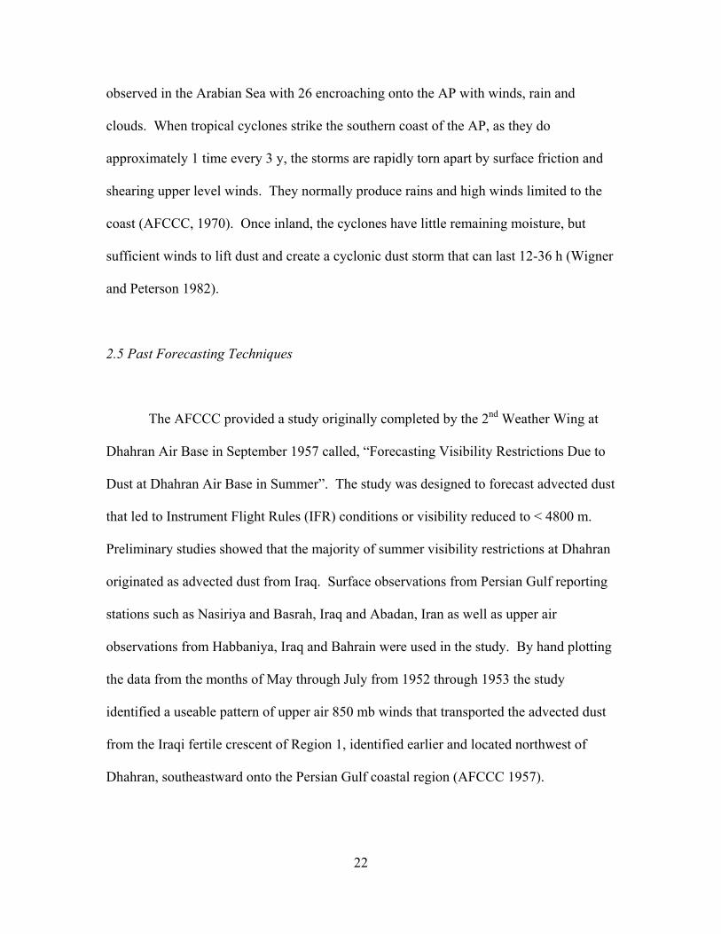
2.5 Past Forecasting Techniques
The AFCCC provided a study originally completed by the 2nd Weather Wing at
Dhahran Air Base in September 1957 called, “Forecasting Visibility Restrictions Due to
Dust at Dhahran Air Base in Summer”. The study was designed to forecast advected dust
that led to Instrument Flight Rules (IFR) conditions or visibility reduced to < 4800 m.
Preliminary studies showed that the majority of summer visibility restrictions at Dhahran
originated as advected dust from Iraq. Surface observations from Persian Gulf reporting
stations such as Nasiriya and Basrah, Iraq and Abadan, Iran as well as upper air
observations from Habbaniya, Iraq and Bahrain were used in the study. By hand plotting
the data from the months of May through July from 1952 through 1953 the study
identified a useable pattern of upper air 850 mb winds that transported the advected dust
from the Iraqi fertile crescent of Region 1, identified earlier and located northwest of
Dhahran, southeastward onto the Persian Gulf coastal region (AFCCC 1957).

23
A simplified version of the technique basically states that if there is no dust
reported upstream, Visible Flight Rules (VFR) conditions ≥ 4800 m will prevail at
Dhahran for at least 24 h. More importantly the study revealed that if dust was reported
within Iraq and the 850 mb wind direction at Bahrain was from the northwest to north
and the 850 mb wind direction at Habbaniya was from the northwest that dust would
reduce visibility to IFR conditions for the next 24 h at Dhahran. Their methodology was
simple yet very useful for Dhahran during the SSH. When independently tested during
the summer of 1956 the study recorded a 76% success rate on the 1200 Zulu (Z) forecasts
and an 82 % success rate on the 1800 Z forecasts which surprisingly was the same as a
persistence forecast (AFCCC 1957).
The “Forecasting Visibility Restrictions Due to Dust at Dhahran Air Base in
Summer” (AFCCC 1957) study resulted with the following general comments and hints
of use for Dhahran, can be applied downstream from Iraq and are listed below:
1. The procedure is an objective aid in forecasting reduced visibilities due to the advection of suspended fine dust from Iraq.
2. Suspended dust may occur either with or without strong gusty surface winds and locally blowing sand.
3. IFR weather may result solely from blowing sand due to strong winds at Dhahran and this method gives no assistance in forecasting the wind speed at Dhahran.
4. When suspended dust is the only restriction to visibility, the visibility is usually lowest at approximately sunrise and usually becomes unrestricted by mid-afternoon.
5. When blowing sand also occurs with the advection of dust from Iraq, visibility often remains below 4800 m for the 24 h period. Visibility will most likely show slight improvement between 1700 and 2400 local time.
6. When blowing sand occurs alone, visibility is usually lowest between 1000 and 1500 local time.
7. Wind speed aloft is apparently of little consequence in applying this method; direction alone is the determining factor.

24
8. This method is intended primarily as an aid in preparing a 24 h Terminal Aerodrome Forecast (TAF) at 1200 and 1800 Universal Time Coordinated (UTC), and its applicability at other times have not been tested.
Many of the rules of thumb from AFCCC (1957) are used to derive the statistical predictors discussed later within this study in the methodology section. The AFWA also addressed dust storm generation in a recently updated
Meteorological Techniques Guide, AFWA Technical Note (TN) 98/002 (Mireless et al.
2002). The guide updated past studies and incorporated general rules of thumb, lessons
learned and research results while addressing forecasting challenges specific to military
meteorologists in three areas such as: surface weather elements, flight weather elements
and severe weather. Under the Visibility Forecasting Rules of Thumb, Dry Obstruction
section, TN 98/002 stated that after dust is already generated and held aloft, wind speed
becomes important in the advection of the dust. “Dust may also be advected by winds
aloft when surface winds become weak or calm” (Mireless et al. 2002). They found that
the duration of a dust event is a function of vertical depth of the dust and the advecting
wind speeds. Mireless et al. (2002) also noted that “forecasting dust generation is more
difficult than forecasting the advection of observed dust into the area.” The data within
Table 2 summarizes the complex processes of dust generation and dust advection that the
current research uses to devise the forecasting tool best suited for Al Udeid AB, Qatar.
2.6 Current Forecasting Techniques
Due to the additional operational needs in support of Operation Iraqi Freedom

25
TABLE 2. Conditions favorable for the generation and the advection of dust. (Adapted from AFWA/TN 98/002) Parameter or Condition Favorable for Dust Generation When for Dust Generation Location with respect to source region Located downstream and in close proximity Agricultural practices Soil left unprotected Previous dry years Plant cover reduced Wind speed ≥ 15.4 m s-1
Wind direction Southwest through northwest (dust source upstream) Cold front Passes through the area Squall line Passes through the area Leeside trough Deepening with increasing winds Thunderstorm Mature storm in local area or generates blowing dust upstream Whirlwind (dust devil) In local area Time of day 1200 to 1900 L Surface dewpoint point depression ≥ 10˚ C Parameter or Condition Favorable for Dust Advection When for Potential Dust Advection Wind speed ≥ 5.1 m s-1 Wind direction Along trajectory of the generated dust Synoptic situation Ensures the wind trajectory continues to advect the dust
(OIF) and Operation Enduring Freedom (OEF) in Afghanistan, the United States Air
Force and Navy has stepped up efforts this year to field operationally tested aerosol
transport models and dust specific satellite imagery enhancements. The AFWA in a joint
project with John Hopkins University’s Applied Physics Lab has taken the University of
Colorado, Boulder division’s Community Aerosol Research Model from Ames/NASA
(CARMA) and combined it with AFWA MM5 model output and called it the Dust
Transport Application (DTA). The DTA model is designed to forecast synoptic scale
dust events within SWA as shown in Fig. 6. In an independent study, Barnum et al.
(2003) discovered that the DTA can successfully forecast synoptic scale dust storm
occurrences throughout SWA 61% of the time with a 10% false alarm rate. The AFWA
rapidly tested and fielded operationally accessible DTA model outputs by creating an
environmental worldwide web link on their Joint Air Force Army Weather Information

26
FIG. 6. Typical DTA output. 26 March 00Z run successfully forecasted a significant
dust storm that affected Qatar on 26 March 2003. (Provided by AFWA/DNXT 2003) satellite imagery and detailed regional dust event discussions. Additionally JAAWIN
Network (JAAWIN). This site provides daily DTA model updates with forecasts out to
72 h, dust highlighted satellite imagery and detailed regional dust event discussions.
Additionally JAAWIN provides a DTA tutorial link to train new users on the capabilities
as well as the limitations of the DTA model outputs. The tutorial mentions that the DTA
model’s most pronounced limitation is the size of the model grid resolution compared to
size of the terrain features and identified dust source regions.
Much of the DTA’s successes of prediction can be attributed to the diligent work
of Dr. George Ginoux and his staff at the Georgia Institute of Technology. His team
utilized Advanced Very High Resolution Radiometer (AVHRR) and Total Ozone
Mapping Spectrometer (TOMS) data to painstakingly map dust source regions from
27
Africa through China. Ginoux’s identified sources represent the majority of observed
regions, but due to the soil type sensitivity and horizontal scale limitations of the remote
sensors, some of the source regions previously identified in this study are not reflected in
the DTA model outputs (Barnum et al. 2003). Under-analyzed AP source regions result
in a pronounced under forecast of synoptic scale dust storm events within the Saudi
Arabian interior. Ginoux’s dust source identification method identified Region 1, Fig. 1
well; therefore according to Barnum et al. (2003), the forecasting skill of the DTA model
increases to an 81% success rate for areas downwind through Kuwait and along the
Persian Gulf coastal region. The dust storm forecast success rates for synoptic scale
systems are promising to operational forecasters in this region. However, though the
DTA model has tremendous applications at the synoptic level, the 28th OWS forecaster’s
guides and tools for meso-scale dust forecasting in SWA are general and limited in scope.
In addition to the AFWA’s modeling efforts, the Navy Research Lab (NRL) in
Monterey, California launched a two sided assault on the dust storms in this region. The
Navy’s aerosol models include the global NAAPS and a newer version of the COAMPS
with a meso-scale aerosol prediction capability. The NRL created a highly accessible
aerosol website that allows the end user to select the world region of interest, the model
of interest, NAAPS or COAMPS 4-panel output with a 48 h NAAPS and a 72 h
COAMPS outlook and loop. The website also has links to current satellite imagery as
well as archived model output.
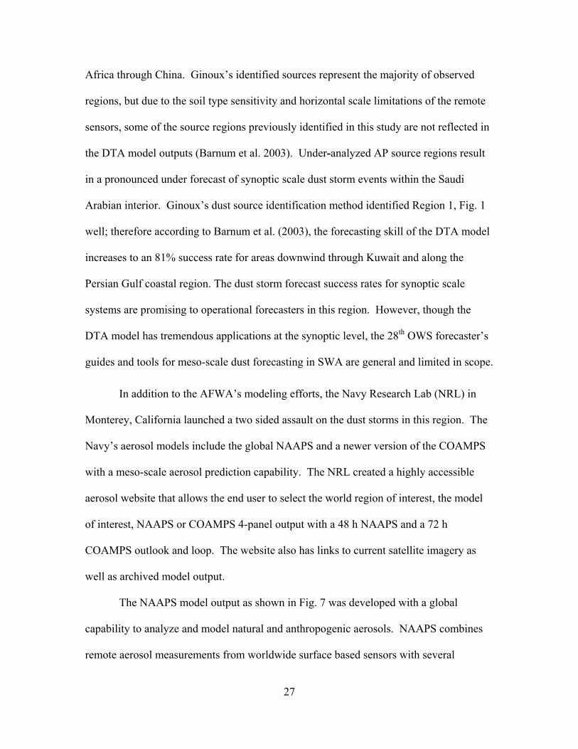
The NAAPS model output as shown in Fig. 7 was developed with a global
capability to analyze and model natural and anthropogenic aerosols. NAAPS combines
remote aerosol measurements from worldwide surface based sensors with several

28
geostationary and polar orbiter remote sensing platforms that monitor daily aerosol
fluctuations and Navy Global Atmospheric Prediction System (NOGAPS) weather
forecasts to produce the regional and global scale aerosol forecasts. The NRL ingests
data from many sources in countless spatial and temporal scales and there remain many
FIG. 7. Typical NAAPS output. 26 March 00Z run successfully forecasted a significant dust storm that affected Qatar on 26 March 2003. (Provided by NRL 2003)

29
challenges to overcome. Some of these challenges include but are not limited to
determining the altitude of identified aerosols, identification and characterization of the
source regions, conversion of synoptic observations to aerosol concentration and
combining the data streams into common format (NRL 2003). Because of the scale of
the challenges to the current NAAPS processing procedures, the previously introduced
NAAPS outputs remain in the development stage, are not always available and are not
operationally tested. However when available the NAAPS outputs can provide an
additional valuable synoptic scale tool for dust forecasting in Qatar (NRL 2003).
The COAMPS mesoscale aerosol model output shown in Fig. 8 is a recent
addition to standard Navy model outputs that started development in 1977 when
COAMPS was designed as a short term, 72 h, meso-scale forecast tool for any region on
the earth. Because the NRL has utilized COAMPS for so long, it is considered a reliable
and stable model output that has many derivations and applications from the synoptic
down to the micro-scale. Expansion of COAMPS into an aerosol transport platform was
a natural progression of this meso-scale output, however the current aerosol model output
has not been field tested and is provided to field units for additional dust forecasting
guidance only.
Additionally, the Marine Meteorology Division at NRL under the guidance of Dr
Steve Miller devised a breakthrough technique that rapidly downloads, reprocesses, and
enhances dust signatures on high resolution satellite imagery from the Moderate
Resolution Imaging Spectroradiometer (MODIS) instrument onboard the Earth
Observing System (EOS) Terra and Aqua polar orbiting satellites. The enhancement
process is limited to visible images and uses algorithms to combine infared and high

30
FIG. 8. Typical COAMPS output. 26 March 00Z run successfully forecasted assignificant dust storm that affected Qatar valid 27 March 2003. (Provided by NRL 2003)
resolution visible channels as well as false color enhancements to discern between cloud
cover and surface based dust (Miller et al. 2003). The operational products are provided
by the Fleet Numerical Model Operations Center (FNMOC) to the end user through a
one-stop secure website known as “Satellite Focus” and shown in Fig. 9 (Miller et al.
2003). “Satellite Focus” provides, regionally focused images, looping capabilities,
multiple atmospheric phenomena enhancements, forecasted satellite passes and product
tutorials. The resulting satellite products have been operationally tested and have

31
FIG. 9. “Satellite Focus” options menu. (Provided by NRL 2003)
successfully supplied valuable dust event enhancement imagery for operators in SWA
supporting OEF and OIF (Miller et al. 2003). Perhaps most impressive are the color dust
enhancement images as seen in Fig. 10; which though limited in temporal scale, clearly
enhance dust events over land or water revealing major as well as minor dust events.
These satellite download procedures and products have been under development since
September 11, 2001 (Miller et al. 2003). The satellite products highlighted in Figs. 9 and
10 have been operationally tested and have successfully supplied valuable dust event
imagery for operators in this region supporting OEF and OIF. As a final note, the
FNMOC has been using all three NRL model and satellite images in conjunction with the
AFWA DTA products mentioned earlier to discuss daily dust outlooks, areas of interest
and model comparisons. These discussions are expected to be expanded to other

32
FIG. 10. High resolution true color MODIS imagery and dust enhancement imagery. (from Miller 2003)
agencies through secure FNMOC web channels with time (Liu et al. 2003), and suggest
an operational release in the near future.
2.7 Regional Study Summary
With the current forecasting techniques addressed, this review focuses on
summarizing some of the more recent regional dust studies completed. The three
regional studies by Bukhari (1993), Safar (1980), and Rao (2001), encompass over 50 y
of surface observations for Saudi Arabia, Kuwait and Qatar respectively. Figure 11
graphically summarizes the studies by highlighting patterns showing seasonal peaks of
dust storms and Shamal winds beginning in March then increasing into June and July
during the SSH. Bukhari (1993) compiled the Saudi Arabian Meteorological and

33
FIG. 11. Mean dust storm/Shamal occurrence for Saudi Arabia, Qatar and Kuwait. (Derived from Bukhari 1993, Rao, et al 2001 and Safar 1980).
Environmental Protection Administration data that consisted of satellite imagery and
hourly surface observations from 8 Saudi Arabian weather stations over a 12 y period
while studying dust events. In a similar study completed over 10 y at the Kuwaiti
International Airport, Safar (1980) concluded that comparable spring and summer dust
event peaks occurred within Kuwait. The most recent study completed by Rao et al.
(2001), noted that over a 28 y period from 1962-1990 the Doha International Airport data
also showed a similar seasonal distribution. Figure 11 shows that on average, Kuwait
recorded the most dust storms within this region, followed by Qatar then Saudi Arabia.
The number of reported storms and differences among the countries show a direct
Normalized Dust/Shamal events
0.0
2.0
4.0
6.0
8.0
10.0
12.0
14.0
16.0
Dec Jan Feb Mar Apr May Jun Jul Aug Sep Oct Nov
Month
Mon
thly
ave
rage
num
ber o
f dus
t/Sha
mal
day
s
SA avg dustKuwait DustQatar Shamal

34
correlation to each country’s proximity to the primary dust source regions. The summer
maximums common to each country depicted within Fig. 11 show that the dust storms
are dependent on sparsely vegetated and dry soil source regions within Iraq and the AP,
intense summer solar radiation and sustained surface winds common during the Summer
Shamals. Finally, Fig. 11 provides the reader with a yearly outlook of trends and focuses
the research on operationally significant seasonal dust storm events that affect Qatar.

35
III. Methodology
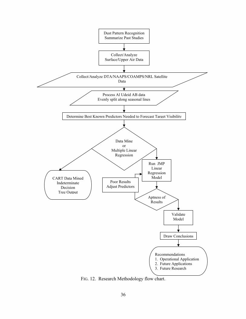
3.1 Overview
Greatly reduced surface based horizontal visibility is a crucial and measurable
hazard affecting operations during dust storms. Developing a mesoscale forecasting tool
that facilitates accurately forecasting these dust storms in Qatar is the main purpose of
this study and involves five distinct processes. First, seasonal dust patterns are
recognized through past data studies. Then, years of surface and upper air data from
surrounding stations are collected and analyzed for climatological and dust advection
patterns. Next, model output are archived from NAAPS, COAMPS and DTA models and
compared with surface observations and MODIS satellite imagery to determine their
ability to forecast and detect dust storm events. Then the dust data is grouped by location
and the Al Udeid AB data is split evenly along seasonal lines and finally evaluated
through CART decision trees and JMP derived multiple linear regression models to show
how each parameter affected surface visibilities at Al Udeid AB, Qatar. The five step
process is illustrated in the methodology flow chart depicted in Fig.12 and is described
below.
First, seasonal and diurnal dust storm peaks and lulls are identified and
understood by analyzing past regional studies. Figure 11 provides a graphical summary
of the primary regional studies reviewed. Additionally the literature review reveals that
sustained winds blowing at 10 m s-1 can lift sufficient dust into the air to reduce visibility
in most cases and initiate a dust event. This correlates well with current dust forecasting
36
FIG. 12. Research Methodology flow chart.
Collect/Analyze Surface/Upper Air Data
Data Mine or
Multiple Linear Regression
CART Data Mined Indeterminate
Decision Tree Output
Determine Best Known Predictors Needed to Forecast Target Visibility
Aptness ofResults
Run JMP Linear
Regression Model
Poor Results Adjust Predictors
Validate Model
Draw Conclusions
Recommendations 1. Operational Application 2. Future Applications 3. Future Research
Collect/Analyze DTA/NAAPS/COAMPS/NRL Satellite Data
Process Al Udeid AB data Evenly split along seasonal lines
Dust Pattern Recognition Summarize Past Studies

37
guidance from the 28th OWS for weather stations in the region, which require a minimum
sustained wind speed at 13 m s-1 to restrict visibility to 4800 m at most locations.
Once the seasonal peaks are identified, surface and upper air data are collected
from surrounding reporting stations such as Al Jaber, Kuwait, Dhahran, Saudi Arabia, as
well as Doha, and Al Udeid AB, Qatar encompassing data packages ten to thirty years
long from the AFCCC. The collected data in comma delineated format is read into
spreadsheets (e.g. EXCEL), where dust events are identified and analyzed for
climatological and advection patterns.
Al Udeid AB operations have been limited to the past 2 y. Therefore once the
seasonal and climatological patterns are established, the archived model output and
satellite imagery for the past 2 y are evaluated to compare the model forecasts and
surface observations and to provide additional relevant predictors for the subsequent
regression analysis. Focusing on data collected throughout the whole year allows this
study to evaluate the numerical and statistical model output through 2 y of known dust
event peaks comprising the winter and summer seasons. As noted in the literature review,
dust storms are the most intense in horizontal extent and duration during these two
distinct winter and summer patterns and should be easily identified within the model
output and enhanced satellite imagery collected.
The next step within the process is to pull the Al Udeid AB dust event data from
the larger data pool, split the collected data evenly and statistically analyze the events.
The Classification and Regression Tree (CART) software was originally used to identify
relevant classification patterns, predictors and decision trees, but the results were difficult

38
to comprehend. Therefore the data is processed through JMP statistical analysis software
to establish the best multiple linear regression analysis models. The resultant statistical
analysis yields an “optimum” regression fit model that incorporates past studies of
seasonal and diurnal patterns, model and satellite interactions as well as surface and
upper air parameters and the accompanying synoptic weather patterns necessary to
produce dust storms while accurately predicting the resultant reduction of visibility.
The closing process of this thesis is to summarize the statistical results and
finalize a semi-automated forecast decision aid that is easily attainable and statistically
proven against known dust events. The resulting decision aid will ultimately allow
forecasters with limited regional weather knowledge to utilize the decision aid in
conjunction with the AFWA and NRL products to easily identify and forecast mesoscale
dust storm development at Al Udeid AB, Qatar in order to reduce the adverse effects of
such weather phenomena on daily operations.
3.2 Past Data
To start, seasonal dust storm peaks and lulls are identified and understood by re-
analyzing past regional studies that are discussed and summarized in detail within the
literature review and Fig. 11. A brief summary of that chapter shows that there are
distinct dust storm event peaks within the winter and summer of studied locations
surrounding Qatar which are attributed to the transitory extra-tropical cyclones in the late
winter/spring and the steady Shamal winds of a SSH. Dust storms are most intense in
horizontal extent and duration during these two distinct seasonal patterns.

39
Additionally, past studies have shown that each studied site is sensitive to wind
direction and the site’s proximity to the major dust source regions. The current research
exploits each reporting station’s dependence on wind speed and direction to show the
importance of the critical upper air and surface data in forecasting future events. Finally
the literature review details valuable rules of thumb and forecasting techniques found in
Table 2 that are instrumental in selecting initial predictors that can be used while
forecasting visibility reductions through statistical linear regression techniques and are
discussed in detail within the results section.
3.3 AFCCC Data
The author requested and received archived comma separated (CSV) surface
observation and upper data from military and international reporting stations from the
AFCCC worldwide database in Asheville, North Carolina. Surface weather observations
are taken and transmitted worldwide every hour at the top of the hour. The military
weather observations used within this study are also recorded and transmitted every hour.
The surface parameters within hourly observations are recorded and transmitted as
follows: time in UTC or Z, wind direction in degrees to the nearest 10˚, wind speed in
whole knots, wind gusts in whole knots, visibility in meters, temperature in degrees ˚C to
the nearest 0.1˚, dewpoint temperature in ˚C to the nearest 0.1˚ and altimeter in inches of
mercury. Due to the expenses of maintaining, launching and recording upper air
soundings, weather balloons are launched only twice a day at 1200 Z and 0000 Z from
upper air sounding reporting stations around the world. The upper air parameters

40
measured are recorded as follows: time in Zulu (Z), atmospheric height measured in m,
atmospheric pressure measured in mb, wind direction in degrees to the nearest 10˚, wind
speed in m s-1, temperature in ˚ C to the nearest 0.1˚, and dewpoint temperature in ˚ C the
nearest 0.1˚. It is also prudent to note that every surface observation reporting station
does not launch upper air sounding balloons. For purposes of research continuity, the
surface and upper wind speeds are converted to m s-1 and maintained in scientific units
throughout. Surface observations are normally available for review a few minutes past
every hour whereas the upper air data may take up to an hour to be processed into useable
form. Both data sources provide crucial information and are incorporated into the global
meteorological models that guide the daily forecasts for cities worldwide.
The surface data collected are analyzed for stations surrounding Al Udeid AB
such as Al Jaber, Kuwait; Dhahran, Saudi Arabia; Bahrain; Doha, Qatar, and Abu Dhabi,
United Arab Emirates and can be found in Fig. 13. The data packages from surrounding
stations span 10-30 y periods, however the data packages received for Al Udeid AB are
limited to the period spanning March 2002 through September 2003 and reflect the short
time that the base has been active. Due to the short data collection period for Al Udeid,
climatological weather data has not yet been generated. The files of hourly observations
from surrounding stations that encompass more than 10 y are large and cumbersome to
analyze. Therefore each file is separated by station and blocks of years, but only data
from 1990 to present are reviewed for this research project.
The surface observations are searched for reported dust in the present weather
column at each station and highlighted accordingly. The highlighting process identifies a

41
significant amount of missing data within Special (off-hour) observations. Often the
missing data can be extracted from the remarks section of the observation while
retrieving data crucial to the research, therefore all of the observations are reviewed by
hand to enhance the accuracy of the study and eliminate possible automation errors. The
restrictions to visibility are then noted with dust events ≤ 4800 m highlighted and bolded.
The highlighted observations from each of the surrounding reporting stations are then
copied and transferred to another spreadsheet. Once the dust events are identified, the
observations and satellite imagery are reviewed to see what environmental conditions
existed before the onset of the dust event and possibly determine if the dust is caused by
local, meso-scale conditions or by larger synoptic scale phenomena. Additionally, each
weather observation preceding the marked events is scrutinized to determine additional
factors such as how recently it had rained, how long it had rained and how many hours or
days after the rain fell was dust able to develop.
Since the Al Udeid AB weather observations began in March 2002, the
surrounding reporting stations are then broken into years, months, days and times that
corresponded with the Al Udeid AB time frame. Then the surface stations are lined up
within the spreadsheet as they fall along the Persian Gulf coast with Al Jaber, Kuwait
first, followed by Dhahran, SA, then Al Udeid AB, Doha and finally Abu Dhabi as noted
in Fig 13. This linear alignment allows a logical analysis of advected dust storms from
Iraq and a quick view of how often dust is advected versus generated locally. Table 2
shows that the underlying physical processes are dramatically different for advected
versus generated dust events. The northwest to southeast alignment, as well as how often
the winds flow from a specific direction and how long they blow before dust onset also

42
provides valuable predictors of dust observed upstream later in the regression analysis
and results sections. The final procedure for the surface observations at this point in the
analysis is to copy and combine the Al Udeid AB observations for both years of the study
into one large spreadsheet and readdress them later once all of the upper air, model and
satellite data are input.
After the surface observations are scrutinized and dust events identified, the upper
level data stations circled in Fig.13 are analyzed for possible patterns within the data.
Geopotential height falls in the upper levels can sometimes signal the onset of advancing
upper level cold air and potentially strong surface winds and are monitored around the
time of each dust event. However, since the majority of the dust events climatologically
occur during the spring and summer months it is noted that height falls are not common
during most SSH events, but should be considered a significant predictor for winter
Shamal events. Additionally, summer radiation inversions, winter frontal inversions and
boundary layer winds within the upper air soundings are reviewed and considered
preceding and during Qatari dust events to determine the factors affecting storm
development and propagation. The outcomes are discussed within the analysis and
results chapter.
The upper air data for the present study are analyzed from the nearest upper air
sounding stations at Dhahran, King Fahad Airport, Saudi Arabia upstream and Doha
Airport, Qatar downstream from Al Udeid and are encircled in Fig. 13. A temporal
problem immediately develops when the upper air data are added to the daily observation
worksheets. Upper air data is available every 12 h, yet surface observations are taken

43
every hour or sooner to note the sometimes rapid changes affecting surface parameters.
Fortunately weather parameters measured above the boundary layer from launched
weather balloons typically change less rapidly than at the surface. The upper air data is
initially matched up with the corresponding times of surface data, then the upper air data
is copied and matched with later surface observations until the next upper air data
becomes available and the process is repeated until each dust event has surface and
corresponding upper air data.
While collecting more recent data used in the analysis for Al Udeid AB there are
many upper air data points that are missing between Dhahran and Doha. To rectify this, a
FIG. 13. Surface and upper level data source stations within SWA. The surface observation points are annotated by red dots with the upper level data points circled. (Adapted from 28th OWS CENTCOM website 2003)

44
statistical comparison between the two reporting stations approximately 128 km apart is
completed. A sample of the statistical results seen in Fig. 14 shows that each
comparative slope from the upper air data recorded between the geographically separated
sounding stations approached 1. Therefore it is concluded that the upper air data from
either station can be used interchangeably with little effect on the final model output.
After the upper air data sets are combined as needed, the remaining few missing days of
upper air data are filled with the FNMOC NOGAPS model output and manually input
into the final spreadsheet. Once the upper air data is lined up by day and time, the upper
air data is combined with the surface observation data in the final spreadsheet for further
analysis with the model and satellite output.
3.4 DTA Data
The DTA model described earlier within the introduction uses a customized
version of the Community Aerosol Research Model from Ames/NASA (CARMA) which
ingests its upper level meteorological and surface terrain parameters from the AFWA
MM5 output while incorporating dust source regions. In an independent study, Barnum
et al. (2003) discovered that the DTA can successfully forecast synoptic scale dust storm
occurrence and propagation in SWA the majority of the time, yet it cannot forecast meso-
scale weather events well.
With these limitations in mind, DTA model output was requested and received
from the AFWA/DNXT DTA model division encoded on a compact disk. The AFWA
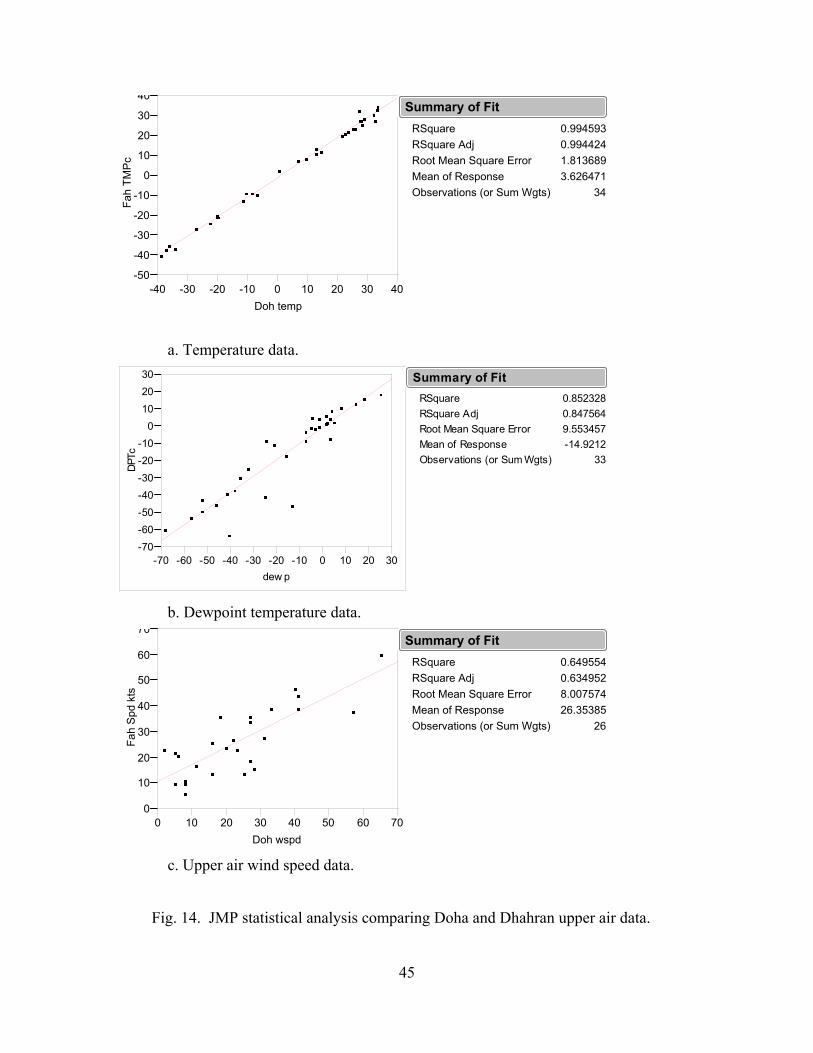
45
-50
-40
-30
-20
-10
0
10
20
30
40
Fah
TMP
c
-40 -30 -20 -10 0 10 20 30 40Doh temp
RSquareRSquare AdjRoot Mean Square ErrorMean of ResponseObservations (or Sum Wgts)
0.9945930.9944241.8136893.626471
34
Summary of Fit
a. Temperature data.
-70-60-50-40-30-20-10
0102030
DPTc
-70 -60 -50 -40 -30 -20 -10 0 10 20 30dew p
RSquareRSquare AdjRoot Mean Square ErrorMean of ResponseObservations (or Sum Wgts)
0.8523280.8475649.553457-14.9212
33
Summary of Fit
b. Dewpoint temperature data.
0
10
20
30
40
50
60
70
Fah
Spd
kts
0 10 20 30 40 50 60 70Doh wspd
RSquareRSquare AdjRoot Mean Square ErrorMean of ResponseObservations (or Sum Wgts)
0.6495540.6349528.00757426.35385
26
Summary of Fit
c. Upper air wind speed data.
Fig. 14. JMP statistical analysis comparing Doha and Dhahran upper air data.

46
provided daily model outputs that started at 0000Z and ended 72 h later at the 1800Z hour
of the third day. The data was received in full color graphical form similar to what can
be used any given day at the JAAWIN environmental website link. A typical output can
be seen in Fig. 6 which encompasses the entire SWA region. The DTA graphical output
is imported into a PowerPoint slide presentation and animated to show the dust storm
forecasted progression and intensity.
DTA’s color coded scale shows the model’s forecasted dust transport
concentrations at 100 m above the ground measured in µg m-³. DTA tutorial guidance
suggests that areas shaded yellow alert users in highlighted areas to the likely transport of
dust with surface visibilities reduced to 4800 m, whereas areas shaded red alert
forecasters to the likelihood of visibilities reduced to 1600 m (Barnum et al. 2003). The
DTA model output is utilized as a first look as to when dust events affect Qatar within the
current years peak dust season from March through September 2003. A dust event is
identified by reviewing the first 4 images of the model, encompassing the first 12-h of the
forecast on days of known dust events. Each day’s model output is encoded within the
master spreadsheet as “forecasted” or “missed” the dust event. The DTA model handles
the majority of the synoptic scale dust events well; therefore the DTA is used as a
predictor within the statistical model.
3.5 NAAPS Data
The NAAPS example model output found in Fig. 7 uses “a predictive, first

47
principle aerosol modeling approach wherein the sources and sinks are theoretically or
empirically derived and depend upon the atmospheric fields forecasted by NOGAPS”
(Liu et al. 2003). NAAPS acquires near real-time aerosol satellite data streams from
AVHRR, TM/Landsat, TOMS and SAGE II polar orbiting and GOES satellites coupled
with a global network of surface based aerosol monitors (AERONET). AERONET has
60 sun-sky monitoring spectral radiometers permanently deployed around the world
including one at Bahrain. The data collected measure optical depth at eight wavelengths
at one minute intervals and can be retrieved via satellite data streams (NRL 2003).
The NAAPS graphical plots found in Fig. 7 are available in two scales, global
scale with the capability of 5-d outlook loops, and a user defined regional scale reduced
to a 2-d outlook loop. These plots are best explained one panel at a time. The upper-left
plot is the optical depth measured at a wavelength of 0.55 microns for three measured
components: sulfate, dust and smoke. The sulfate contours start at 0.01 and double in
magnitude for consecutive contours with the assigned colors varying from orange shades
to red (NRL 2003). The upper-right plot is the sulfate mass mixing ratio measured in µg
mֿ³ at the surface. The contours start at 0.02 and double in magnitude for consecutive
contours with the colors assigned the same as above (NRL 2003). The lower-left plot is
the dust mass mixing ratio and is the plot that is monitored when forecasting dust in this
region. The dust mass mixing ratio is measured in µg mֿ³ at the surface. The dust
contours begin at 20.0 and double in magnitude for consecutive contours with the
assigned colors varying green shades through yellow (NRL 2003). The lower-right plot
is the smoke mass mixing ratio measured in µg mֿ³ at the surface. The contours begin at
0.2 and double in magnitude for consecutive contours with blue shades (NRL 2003).

48
The dust mass mixing ratio is the plot used for verification among the Al
Udeid AB dust events highlighted earlier. A NAAPS dust column is added to the master
spreadsheet and the archived NAAPS dust mass mix ratio outputs are reviewed for signs
of dust during each event through September 2003. Because the environmental
conditions inherent within this desert environment predispose the surrounding
atmosphere with some level of dust year round, the NAAPS plots are closely scrutinized
to determine what dust mass mixing ratio is necessary to reduce surface visibilities to
4800 m. A review of recent NAAPS plots, shows that shades of light green correlate well
with reported dust at the surface reducing visibility to 4800 m. With the shade of green
determined, the daily NAAPS plots are scrutinized on the dates of known dust events at
Al Udeid and subsequent entries are made within the master spreadsheet as “forecasted”
or “missed” the dust events. The NAAPS forecasts a majority of the synoptic events over
the two-year period; therefore NAAPS is used as a predictor within the statistical model.
The NRL discussions of the NAAPS strengths include an integration of real
weather into the model through NOGAPS, extended 120-h outlooks, operation in near-
real-time, and global coverage with dust and smoke simulations (NRL 2003). The noted
areas of work in progress for NAAPS include improvement of dust source functions,
verification of the sulfate simulations and improved microphysics and chemistry. Some
additional NAAPS operational challenges include but are not limited to determining the
altitude of identified aerosols, identification and characterization of the source regions,
conversion of synoptic observations to aerosol concentration and combining the data
streams into a common format (NRL 2003). Despite the many challenges yet to be
solved, the NRL continues to ingest data from multiple sources in countless spatial and

49
temporal scales and produce high quality aerosol guidance for the region. Because of the
large scale of these challenges, the previously introduced NAAPS outputs remain in the
developmental stage, are not always available and are not operationally tested and
verified. However, when available the NAAPS outputs can provide a valuable tool for
dust forecasting in Qatar.
3.6 COAMPS Data
The second NRL aerosol model is the latest version of COAMPS with an aerosol
prediction capability released in March 2003. Similar to NAAPS the COAMPS aerosol
model uses “a predictive, first principle aerosol modeling approach wherein the sources
and sinks are theoretically or empirically derived and depend upon the atmospheric fields
forecasted by COAMPS” (Liu et al. 2003). The COAMPS mesoscale aerosol model
output shown in Fig. 8 is a recent addition to standard outputs that started development in
1977 when COAMPS was designed as a short term, 72 h meso-scale forecast tool for any
region on the earth. Even though the current aerosol model output is not extensively
field-tested, Liu et al. (2003) notes that a COAMPS 72 h forecast successfully covered
the major dust event that crippled the AP from 25 – 27 March 2003 with wind and dust
forecasts throughout the duration of the event. Since its recent inception, the aerosol
COAMPS version is provided to field units for additional dust forecasting guidance only,
though current research shows promise for COAMPS model output plots.
The COAMPS graphical plots as seen in Fig. 8 come in two grid resolution sizes,
81 km and 27 km, with the maximum capability of 72 h outlook loops at 3 h intervals

50
(NRL 2003). The graphical plots are best described one panel at a time. The upper-left
plot represents the surface friction velocity patterns measured in cm sֿ¹ in the form of
blue stream lines with surface soil moisture measured in shades of green for dry to
magenta for moist. The upper-right plot represents dust surface concentrations and is the
plot of greatest interest when forecasting dust in this region, whereas COAMPS uses a
threshold of 65 cm sֿ¹ for dust lifting (NRL 2003). Initially the dust concentrations were
measured in mg mֿ³ and coded in colors from blues for small concentrations to magenta
for high concentrations of aerosols through the end of the 26 March 0000 Z model run.
Figure 15 shows that starting March 27 at 0000Z, 2003 the dust concentration plots were
changed to measure in µg mֿ³ to match standard mass mixing ratio measurement units
while the color codes were shifted to 4 shades of color from blues for small
concentrations to magenta for high concentrations. The lower-left plot is the dust optical
depth coded in colors from blues to purples and has no units. The lower-right plot is
similar to the NAAPS plot of the same position, but called the oil smoke mass loading
measured in mg mֿ² at the surface and coded in colors as above with blues representing
minute smoke loads through purple for extreme smoke loads. The oil smoke loading plot
was discontinued 26 April 2003 (NRL 2003).
Similarly to the quandary that arose while reviewing NAAPS plots, the
environmental conditions inherent within a desert environment predispose the
surrounding atmosphere with some level of dust year round. The COAMPS plots are
closely scrutinized to determine the dust mass mixing ratio necessary to reduce surface
visibilities to 4800 m. A review of recent COAMPS surface dust concentration plots

51
shows that shades of green are positive indicators of dust reported at the surface reducing
visibility to < 4800 m. The upper-right plot of dust mass mixing ratio is the plot used for
verification among the Al Udeid AB dust events highlighted earlier. A COAMPS dust
column is added to the master spreadsheet and the archived COAMPS dust mass mix
ratio outputs are reviewed for signs of dust as green shading during each event through
September 2003 and noted within the spreadsheet. The COAMPS model forecasts a
majority of the synoptic events over the two-year period; therefore COAMPS is used as a
FIG. 15. Latest COAMPS dust concentration plot. Rescaled to µg mֿ³. (Provided by
NRL 2003)

52
predictor within the final statistical model. Because of the recent release of the
COAMPS aerosol version, the previously discussed COAMPS plots remain in the
developmental stage, are not always available and are not operationally tested and
verified. However when available the COAMPS outputs can provide an additional tool
for dust forecasting in Qatar.
3.7 Satellite Focus Data
The final NRL product used within the research to identify dust storm signatures
is the “Satellite Focus” website which recently supplied and sustained deployed
personnel with high quality satellite imagery. With the numerous successes of the
“Satellite Focus” website, Dr. Miller and his staff have met the DoD task for the research
community to become more “proactive” and “forward-focused” by pushing the
technological envelope and fielding accessible, reliable and high quality satellite products
that can directly enhance warfighter capability (Miller 2003).
A satellite dust column is added to the master spreadsheet and the archived
satellite imagery outputs are reviewed for signs of dust during each event through
September 2003 and noted within the spreadsheet. The enhanced archived satellite
imagery detects a majority of the noted dust events over the two-year period; therefore
the satellite imagery is used as a predictor within the final statistical model.

53
3.8 Data Splitting
With all of the past study knowledge, surface and upper air data, as well as model
outputs and satellite imagery entered into the master spreadsheets, the data are split for
regression analysis. Neter et al. (1990) notes that the best method to test and validate a
regression analysis is to design the model with a test data set and validate the model by
generating an independent validation data set. They also note that generating new data
for validation is often not a valid option due to research limitations. Because generating a
validation data set within the current research is feasible, the data sets within the master
spreadsheets are separated into a test and validation data set.
There are many theories on how to best separate data when new data cannot be
generated to test the validity of the regression model. Random divisions, 80/20, 60/40
and 50/50 data splits are all valid options, but for this investigation the database is split
evenly. According to Neter et al. (1990), when seasonal data or cyclical events are being
analyzed, such as seasonal dust storms, the data can be split as long as the remaining data
sets are balanced. Therefore the data for this research is split and balanced such that dust
events within each month or season are approximately equally represented within each
data set. The new spreadsheets are renamed “test” and “validation” data set accordingly,
and are put aside for further statistical analysis.

54
3.9 CART Data
As a test of its possible utility, a data mining technique using Classification and
Regression Tree (CART) software is introduced to the research process. CART is
designed to provide simplified decision trees based on specific statistical data splitting
techniques that can evaluate thousands of multiple variables; categorize them into order
of importance based on degree of changes in the data, and then split the data into
branches of occurrence or non-occurrence at the point of CART defined most significant
difference. CART continues the technique until the splits of data can no longer be
completed due to lack of significant parameters to split (Salford Systems 1995). The
CART process requires that data be pre-analyzed into classification categories of simple
decisions. This allows the preliminary results to force a focus on the primary predictive
targets that had been successful predictors in the past.
Using this technique, the CART program claims to simplify large sized,
complex data patterns into easily identified general patterns of decision trees that help
determine specific conditions necessary for identified event occurrence (Salford Systems
1995). Initially, CART requires multiple parameters of interest in order to prune the
decision trees down to specific parameters of interest that isolate the current research
target of reduced visibility. Unfortunately, within this research, CART produces very
large preliminary decision trees with complex branches of parameter interaction that tend
to split on seemingly random values within the predictor parameters. Because the initial
CART decision trees are difficult to decipher with multiple splits of little physical

55
meaning, this study focuses on a multiple linear regression analysis to provide a more
direct and interpretable solution.
3.10 Multiple Linear Regression
Many problems in the scientific community involve investigating relationships
between two or more physical variables. These relationships can be analyzed through
multiple linear regression techniques, but only after assumptions about the data
population are made. For this research, data spanning almost two years from March 2002
through September 2003 are analyzed. Because the study focuses on dust events that
reduced the surface visibility to ≤ 4800 m, the two year data base is reduced to 64
significant dust events, but among those 64 events there are 465 weather observations
recorded. From the central limit theorem of statistics, a sample of data whose numbers or
observations exceed 30 -- and are taken from a population that has an unknown
probability distribution – is likely to result with a sample mean that is approximately
normal (Montgomery and Runger 2003). Additionally the weather observations collected
and used to develop the model are assumed to be independent of one another. The linear
regression model’s predictive parameters and resultant residuals are also assumed to be
normally distributed random variables with common variance. Normality can be verified
graphically by computing random scatter and normal plots of the residuals once the final
model is derived, and is further discussed within the analysis and results chapter.

56
Multiple linear regression analysis is a statistical technique used to show the
linear relationship between a response and multiple predictors and is chosen as the most
effective statistical analysis for the current research. The research shows that as the
number of predictors or weather parameters increases, the linear reaction with the
response or predicted reduced surface visibilities becomes more intricate but can be
solved through multiple linear regression techniques. The research goal of forecasting
reduced surface visibilities can be described statistically with visibility measured in
meters as the response variable or predictand, and the observed weather parameters and
model inputs as the regressors or predictors. This can be represented by linear Eq. 1,
Y β 0 β 1 X 1⋅+ ......β n X n⋅+ ε+ (1)
where Y is the response variable, visibility; β0 the intercept or “regression constant”; βn
“regression parameters”, and Xn the variables or predictors with ε, residuals, assumed as
the resulting random error with a mean of 0 and an unknown variance (Wilks, 1995).
Wilks (1995) also notes that the residuals “correspond geometrically to the distance
above or below this surface along a line perpendicular to the (X1, X2) plane.” The
positive multiple linear regression results achieved are relatively easily derived and
understood. These results are also readily repeated through simple computer programs
that can be forwarded to the end user. Therefore multiple linear regression is the
statistical method chosen to best predict reduced surface visibility.
3.11 JMP Data
The aforementioned model and satellite imagery data are entered into the final

57
spreadsheets as valid predictors in the final linear regression model. The software used
for the creation of the linear regression model is called “JMP”. The JMP software
package is designed by the SAS Institute as a “Statistical Discovery Software” widely
used in advanced academic settings and industries worldwide. Once the surface and
upper air data are effectively sorted within the spreadsheet and all parameters known to
affect the surface visibility are included, the data is entered into JMP. Once opened in
JMP, the final data files are scanned visually for occasional data points that are dropped
when transferring from the spreadsheet software. In order to maximize the data points
collected over the 2 y study period, dropped values are re-entered and saved. The JMP
software allows a semi-seamless conversion from the spreadsheet software to efficiently
evaluate dust event distributions such as maximums, minimums, means and trends of
interaction between predictors and response parameters. In order to derive the dust storm
distributions, a JMP “Fit Y by X” graphical option is invoked where the target variable of
reduced visibility is compared with each surface observation parameter reported to
determine the effect of each parameter on the visibility within all dust storm events.
These data distributions are discussed in detail in the analysis and results chapter.
After the files are prepped, JMP is used to establish an “optimum” regression
analysis to simplify the environmental predictors necessary to accurately forecast
reductions in visibility and to determine specific conditions necessary for identified event
occurrence. The most efficient way to achieve an “optimum” regression model is to use
the Fit Model option.
Since the data population is seasonally split into separate test and validation data
sets, the Fit Model is first applied to the test data set. The test data set is opened within

58
the Analyze Fit Model option as depicted in Fig. 16. The visibility parameter is entered
as the Y or response variable the model tries to predict. The remaining parameters drawn
from the columns of the test data set spreadsheet are then added to the model effects
column or predictors as needed to fine tune the model.
The coefficient of determination (R²) value is often used as a measure of the
model adequacy in capturing the overall variability of the model. An R² of 1 would
indicate a perfect model that predicted the response variable without variability. There is
no limit to the number of predictors allowed within the fit model, however, in order to
prevent over-fitting the test data set, the final predictors chosen are limited to field-
accessible, meteorologically sound predictors such as satellite and dust model data,
surface observations and upper air data. A Fit Model utilizing the primary predictors as
seen in Fig.16 produces R² values climbing into the 0.70s. Including cross product
interactions increases the response accuracy to R² values in the low 0.90s. To better
understand multiple predictors and their interactions, the JMP derived R² adjusted
statistic is also monitored. The R² adjusted statistic is a tool noted in Montgomery and
Runger (2003) that lowers the R² value by the degree of over-fitting caused by too many
predictors.
In addition to the R² values and the R² adjusted values, JMP standard Fit Model
output shows Parameter Estimates which list each predictor and the statistical analysis of
its performance within the model. Cross products whose Probability > t values exceed
0.20 are removed one at a time to improve both R² and RMSE values. This procedure is
repeated until an “optimum model” is achieved. A final Forward Step Wise model run is
then executed using 0.20 values as probability values to enter the model and 0.10 values

59
FIG. 16. JMP Fit Model interface. Used when creating standard least squares or stepwise models. (derived from JMP 2003)
to leave the model to eliminate predictor redundancies, simplify the model by cutting the
total number of predictors from 90 to 53, and reinforce the validity of the initial model
assumptions. With the R² value optimized for the test data set, the procedure is then
applied to the validation data set with results discussed in the next chapter.

60
IV. Analysis and Results
4.1 Introduction
The previous chapter discussed the methodology used to sort, group, split equally
along seasonal lines and analyze the data to develop an optimized fit model for the test
data set that accurately forecasts the reduction of visibility due to dust-producing
environmental conditions. The next 4 sections discuss the statistical analysis of
significant dust events occurring during the study period, the optimized fit model
developed with the test data set, the results of the fit model applied to the validation data
set, and finally operational applications of the model.
4.2 Statistical Dust Event Analysis
An analysis of all the dust events affecting Al Udeid over the past 2 years reveals
a spectrum of severity in dust storm phenomena. To quantify a physically meaningful
dust storm threshold, a 3-step filter is applied to the events. First the study addresses the
number of dust events occurring since Al Udeid AB began recording surface observations
in March 2002 through the end of the study in September 2003. Secondly the research
investigates the number of advected dust events that originate upstream compared to the
number of dust events that are generated locally, and the different environmental
conditions that foreshadow each type of event. Finally, the study addresses the monthly
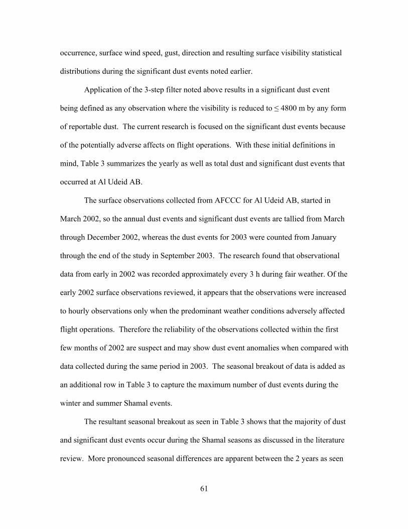
61
occurrence, surface wind speed, gust, direction and resulting surface visibility statistical
distributions during the significant dust events noted earlier.
Application of the 3-step filter noted above results in a significant dust event
being defined as any observation where the visibility is reduced to ≤ 4800 m by any form
of reportable dust. The current research is focused on the significant dust events because
of the potentially adverse affects on flight operations. With these initial definitions in
mind, Table 3 summarizes the yearly as well as total dust and significant dust events that
occurred at Al Udeid AB.
The surface observations collected from AFCCC for Al Udeid AB, started in
March 2002, so the annual dust events and significant dust events are tallied from March
through December 2002, whereas the dust events for 2003 were counted from January
through the end of the study in September 2003. The research found that observational
data from early in 2002 was recorded approximately every 3 h during fair weather. Of the
early 2002 surface observations reviewed, it appears that the observations were increased
to hourly observations only when the predominant weather conditions adversely affected
flight operations. Therefore the reliability of the observations collected within the first
few months of 2002 are suspect and may show dust event anomalies when compared with
data collected during the same period in 2003. The seasonal breakout of data is added as
an additional row in Table 3 to capture the maximum number of dust events during the
winter and summer Shamal events.
The resultant seasonal breakout as seen in Table 3 shows that the majority of dust
and significant dust events occur during the Shamal seasons as discussed in the literature
review. More pronounced seasonal differences are apparent between the 2 years as seen

62
TABLE 3. Summary of reported dust and significant dust events at Al Udeid AB. Dust Events Significant Dust Events VSBY ≤ 4800 m
Year 2002 31 17Season Mar-Sep 24 11Year 2003 95 47Season Mar-Sep 47 43
Year Totals 02 and 03 126 64Season Totals 02 and 03 71 54
in Table 3. The dust season of March through September for 2002 yields 24 dust events
that reduced visibility while the dust season for 2003 reports twice as many dust events
with 47. The increase in seasonally significant dust events that reduce visibility ≤ 4800
m is more pronounced, as 11 significant events are reported from March through
September in 2002, yet the same seasonal time frame in 2003 yields 43 significant dust
events -- an approximate 4-fold increase. The reason for the noticeable increase is not
inherently obvious from the data analysis, but a summary of possible solutions follows.
Limited observation reporting hours early in 2002 -- due to fewer military
operations -- could be a source of some of the disparity in that some small-scale, between
observation, dust events not reported in 2002 are reported in 2003. Additionally, the
observation reporting procedures, such as day and night visibility marker locations could
have been under development the first year and standardized the second year. Another
possible source of the yearly difference could be increased anthropogenic activity in the
form of Coalition ground troops who moved from Kuwait and into Iraq early in 2003.
According to Clements et al. (1963) and Prospero et al. (1986), any increased
anthropogenic activity across a source region surface greatly reduces the horizontal
threshold velocity required to lift dust particles into the air. Therefore as tens of

63
thousands of Coalition troops in support of OIF drove across Kuwait and into southern
Iraq during early spring of 2003, the desert source regions were likely disturbed, thereby
providing additional dust sources. Another potential culprit for the yearly disparity could
be increased farming along the fertile crescent of the Tigres and Euphrates river valley in
southern Iraq due to the policy of the past government to drain the marshes in the region
for agricultural use.
The literature review documented a higher wind threshold of 15 m s-1 for dust
generation than for dust advection at 5 m s-1. For this study a generated dust event is
defined as an event that occurs locally at the reporting station and is not advected from a
source region upstream based on wind direction. An advected dust event is defined as an
event larger in horizontal and possibly vertical scale, reported upstream at most reporting
stations, and transported downstream by strong surface and upper level winds.
Additionally, dust events categorized by distant or local sources within this section are
evaluated from the beginning of the study period in March 2002 through September
2003.
The data are separated and regrouped into advected dust events that originated
upstream of Al Udeid or are generated locally. Once separated, the data show 103
surface observations capturing 21 significant dust events that are generated locally and
344 surface observations capturing 43 significant dust events that originate upstream and
advect into Al Udeid AB. A brief discussion follows of some of the parameters
monitored during significant dust events that reduced visibility ≤ 4800 m. at Al Udeid
AB. These parameters are summarized in Table 4.
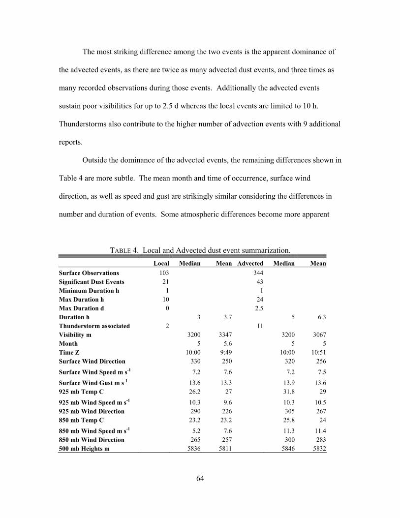
64
The most striking difference among the two events is the apparent dominance of
the advected events, as there are twice as many advected dust events, and three times as
many recorded observations during those events. Additionally the advected events
sustain poor visibilities for up to 2.5 d whereas the local events are limited to 10 h.
Thunderstorms also contribute to the higher number of advection events with 9 additional
reports.
Outside the dominance of the advected events, the remaining differences shown in
Table 4 are more subtle. The mean month and time of occurrence, surface wind
direction, as well as speed and gust are strikingly similar considering the differences in
number and duration of events. Some atmospheric differences become more apparent
TABLE 4. Local and Advected dust event summarization. Local Median Mean Advected Median MeanSurface Observations 103 344 Significant Dust Events 21 43 Minimum Duration h 1 1 Max Duration h 10 24 Max Duration d 0 2.5 Duration h 3 3.7 5 6.3Thunderstorm associated 2 11 Visibility m 3200 3347 3200 3067Month 5 5.6 5 5Time Z 10:00 9:49 10:00 10:51 Surface Wind Direction 330 250 320 256
Surface Wind Speed m s-1 7.2 7.6 7.2 7.5
Surface Wind Gust m s-1 13.6 13.3 13.9 13.6925 mb Temp C 26.2 27 31.8 29
925 mb Wind Speed m s-1 10.3 9.6 10.3 10.5925 mb Wind Direction 290 226 305 267850 mb Temp C 23.2 23.2 25.8 24
850 mb Wind Speed m s-1 5.2 7.6 11.3 11.4850 mb Wind Direction 265 257 300 283500 mb Heights m 5836 5811 5846 5832

65
within the first couple of mandatory upper level layers. For example, a 2˚ C increase in
the mean 925 mb temperature during advected dust events could be a reflection of a
surface based temperature inversion that restricts surface mixing while maintaining
suspended dust near the surface with reduced visibilities. The inversion may also hold
the 1 m s-1 stronger mean winds aloft to continually transport the dust further downstream
through extended dust fallout. The 925 and 850 mb wind directions for local events
show a southwestern trend compared to the more westerly to northwesterly directions of
the advected events. The northwesterly wind direction at the 925 and 850 mb upper
levels was a positive precursor to advected events during the summer dust study at
Dhahran AB, Saudi Arabia (AFCCC 1957). Finally, the strongest difference apparent at
the upper levels is the 850 mb wind speed where the advected events show a mean
increase of 3.8 m s-1 over the local events. Notably, the AFCCC (1957) dust study
claims that wind direction aloft is the main contributor to the advected dust events and
that wind speed is “of little consequence.” However the Dhahran dust study was focused
on SSH events, whereas the current research at Al Udeid AB encompasses yearly dust
events, so the discrepancies noted can possibly be explained by the seasonal restrictions
of the Dhahran study.
Overall, the atmospheric contrasts between locally generated and advection dust
events are subtle and offer little guidance to discern between forecasting local versus
advection events. However, the main points that can be gathered from the dust storm
summary are that advected events occur twice as often, last twice as long, are more
common with stronger northwesterly winds aloft and surface wind gusts whereas local

66
events are more likely to be generated with a southwest to westerly surface component to
stir up surrounding local dust sources for a much shorter period of time.
Finally, a JMP statistical dust event analysis is conducted to address the monthly,
surface wind speed, gust, direction, upper air wind speed, direction and resultant visibility
distributions encapsulating all of the local and advected dust events. A brief description
of each parameter’s distribution follows.
The first distribution of significant dust event parameters analyzed using JMP are
the months of occurrence and can be found in Fig. 17. This bar chart shows a trend
similar to the event distributions seen in Fig. 11 and discussed in Table 4 where March
shows a marked increase with a secondary peak into May. The monthly bar chart within
Fig. 17 is skewed by the number of observations taken in May during an extreme 2.5 d
SSH event; otherwise the distribution follows seasonal patterns apparent in Fig. 11 as
expected.
Figure 18 shows the wind direction distribution during significant dust events and
2 3 4 5 6 7 8 9 10 11 12
Month
23456789101112Total
Level 16 101 58 137 48 23 36 11 2 6 9
447
Count
11 Levels
Frequencies
FIG. 17. JMP monthly distribution of surface observations taken during significant dust events for 2002 and 2003.
67
shows the median or mid point of all recorded wind directions is 320˚ with the mean of
271˚. This wind direction is consistent with the northwest annual mean wind directions
recorded throughout the region.
The third distribution of observed dust event parameters analyzed is wind speed
as shown in Fig. 19. The wind speed distribution shows that during the significant dust
events recorded, the maximum sustained wind speed is 17.99 m s-1 with the minimum
recorded as calm winds. The median or mid point of dust event wind speeds is 7.2 m s-1
with the mean at 7.5 m s-1. This mean wind speed is consistent with winds required to
advect dust defined earlier as 5 m s-1 and stronger than the climatological wind speeds
recorded at nearby Doha International Airport that shows an annual mean wind speed of
5.7 m s-1 (AFCCC 2003).
The fourth distribution of dust event parameters analyzed is wind gusts as shown
in Fig. 20. The wind gust distribution shows that wind gusts were recorded at only 323
of the 447 significant dust event observations. The reduced number of recorded gusts
0 100 200 300
100.0%99.5%97.5%90.0%75.0%50.0%25.0%10.0%2.5%0.5%0.0%
maximum
quartilemedianquartile
minimum
360.00 360.00 360.00 340.00 340.00 320.00 260.00 60.00 12.00 0.00 0.00
QuantilesMeanStd DevStd Err Meanupper 95% Meanlower 95% MeanN
270.91723105.89279 5.008557280.76053261.07392
447
Moments
WD
FIG. 18. JMP wind direction distribution of surface observations taken during significant dust events for 2002 and 2003.

68
0 10
100.0%99.5%97.5%90.0%75.0%50.0%25.0%10.0%2.5%0.5%0.0%
maximum
quartilemedianquartile
minimum
17.995 16.843 14.910 12.339 10.283 7.198 5.141 3.085 1.028 0.000 0.000
QuantilesMeanStd DevStd Err Meanupper 95% Meanlower 95% MeanN
7.49009393.55903440.16833657.82092537.1592626
447
Moments
Surface Wind Speed m/s
FIG. 19. JMP wind speed distribution of surface observations taken during significant dust events for 2002 and 2003.
indicates the sporadic nature of wind gusts. The maximum wind gust shown is
23.65 m s-1 with a minimum gust recorded at 6.2 m s-1. The median or mid point of
recorded wind gusts is 13.88 m s-1 with the mean at 13.6 m s-1. Wind gusts are described
within the literature review as a necessary forcing mechanism to lift the dust into the air
as well as turbulently mix the dust near the surface.
The final distribution of dust event parameters analyzed, the surface visibility
10 20
100.0%99.5%97.5%90.0%75.0%50.0%25.0%10.0%2.5%0.5%0.0%
maximum
quartilemedianquartile
minimum
23.650 23.650 19.537 18.509 16.452 13.882 10.283 8.740 7.198 6.170 6.170
QuantilesMeanStd DevStd Err Meanupper 95% Meanlower 95% MeanN
13.5984153.75305230.208825414.009249 13.18758
323
Moments
Surface WG m/s
FIG. 20. JMP wind gust distribution of surface observations taken during significant dust events for 2002 and 2003.

69
distribution is the primary focus of this investigation and is illustrated in Fig. 21. The
visibility distribution shows that during significant dust events, the maximum visibility is
at 4800 m with the minimum reduced to 200 m. The median or mid point of dust event
visibilities is 3200 m with the mean of 3127.5 m. The mean visibility of 3127.5 m is a
direct result of the mean wind direction from the west at 271˚ coupled with the mean
wind speed of 7.49 m s-1. The mean wind direction and wind speed are also consistent
with wind directions and speeds required to advect dust defined earlier as northwesterly
wind directions and wind speeds of at least 5 m s-1.
Both the mean direction and wind speed results are slightly different from past
guidance. The literature review noted that most reporting stations in the AP region
require a more northwesterly flow and stronger winds closer to 13 m s-1 to reduce
visibility. Additionally the mean wind speed at 7.49 m s-1 is lower than past forecast
guidance from the 28 OWS (2003) that sets a 13 m s-1 threshold to reduce visibility to
4800 m. Hence the differences inferred from this study suggest that the increased activity
0 1000 2000 3000 4000 5000
100.0%99.5%97.5%90.0%75.0%50.0%25.0%10.0%2.5%0.5%0.0%
maximum
quartilemedianquartile
minimum
4800.0 4800.0 4800.0 4800.0 4800.0 3200.0 1800.0 960.0 600.0 324.0 200.0
QuantilesMeanStd DevStd Err Meanupper 95% Meanlower 95% MeanN
3127.51681419.492467.1396863259.46622995.5673
447
Moments
VSBY m
FIG. 21. JMP visibility distribution of surface observations taken during significant dust events for 2002 and 2003.

70
at Al Udeid AB over the past two years has both enhanced dust suspension and improved
dust reporting.
The dust storm distribution and analysis of key parameters discussed previously
show the importance of many of the key surface predictors and their roles in visibility
reduction. The primary predictors that are used to finalize the model are chosen with
consideration of past studies, trial and error tests within the model, and their availability
to the operational forecaster. These predictors are listed below in order of model
appearance: month, time, surface wind direction (WD), surface wind speed (WS), surface
wind gust (WG), surface altimeter, DTA forecasted dust, NAAPS forecasted dust,
COAMPS forecasted dust, satellite imagery depicted dust, dust reported upstream,
surface temperature (T), surface dewpoint temp (Td), 925 mb T, Td, WS, WD, 850 mb T,
Td, WS, WD, 500 mb T, Td, WD, 300 mb T, Td, WS and WD. The remaining predictors
used are derived from cross products of the primary predictors and are listed in Table 7 in
the Appendix.
According to Wilks (1995), transformations of predictors, such as cross products,
can sometimes lead to a better understanding of the physical processes behind the
phenomena being studied. However, Wilks (1995) also notes, that if a better forecast
about the phenomena being studied is the ultimate goal, then the physical processes
involved are sometimes less important than the final outcome. Because the current
research is focused on the forecasted reduction in visibility, a full explanation of the
complex physical interactions is considered unnecessary. Therefore no effort is made to
explain why the 25 cross products introduced within the research increase the validity of
the best Fit Model derived.

71
4.3 Test Data Results
Based on the statistical results of the significant dust storms and the discussions of
the predictors within the previous two sections, a multiple parameter linear regression Fit
Model from the JMP software is obtained using 28 primary predictors coupled with 25
cross product derived predictors shown in Table 7 of the Appendix. This section first
addresses the JMP Summary of Fit results that include R2, R2 adjusted, RMSE, the mean
of the response, a 95% prediction interval, then it discusses the overall F-test results and
finally it discusses the resultant residual plots and how they relate to the validation phase
of the model.
The Summary of Fit statistical results from the “optimum” Fit Model are shown
in Table 5. The R2 value of 0.91 is a highly regarded model output because this implies
this model’s ability to capture 91% of the variance of the outcomes. The R2 adjusted of
0.87 is also desirable since an R2 adjusted statistic near the R2 value indicates the
regression is not over-fit with excessive predictors. The Root Mean Square Error
(RMSE) of 514 m is also encouraging and perhaps the most impressive result as it
suggests the model could provide an operational forecaster a visibility prediction tool
accurate to within 1/3 of a mile.
Given that the RMSE meets the research objective of “accurate to within 800 m,”
the regression fit model is considered optimized. Thus adjustments are halted with a final
test data set Mean of the Response of 2953 m. Mean of the Response or the predicted
visibility is the mean of the best fit model predicted visibility in meters which is used to
compute a 95 % prediction interval. The test data set computed prediction interval or

72
TABLE 5. JMP derived test data model statistical output. Test Data set Summary of Fit R Squared 0.9149R Squared Adj. 0.8684Root Mean Square Error 514.43Mean of Response 2943.05Observations 151Prob > F < 0.0001 Mean Square Error (MSE) 264,640
probability of predicted values falling within that 95% prediction interval is later used to
further determine the adequacy of the best fit model when applied to the validation data.
The observations value is simply the number of surface observations from the test data
set that the model uses while deriving the statistical model output.
The final statistical value computed within Table 5 is the Prob > F which is the
overall F- test or the statistical probability of “obtaining a greater F-value by chance
alone if the model fits no better than the response mean” (SAS Institute 2003). Since
probabilities of F < 0.05 show that there is significant regression within the model being
fit, the Prob > F < 0.0001 value that is derived while fitting the current model offers
further proof that the best Fit Model depicts significant regression and is a model worth
investigating further with additional tests.
The final statistical test to determine the adequacy and reliability of the fit model
developed is to review the Residual plots found in Figs. 22 and 23 to assess the
randomness, heteroscedasticity or non-constant variance and normality of their plotted
patterns (Wilks 1995). Residuals, as discussed earlier, are the difference between the
observed and predicted visibilities. Therefore when the Residuals yield an objectively
random scatter pattern as seen in Fig. 22 and an approximate normal distribution as

73
-1000
0
1000
Res
idua
l0 50 100 150 200 250
Row Number
Residual by Row Plot
FIG. 22. JMP derived test data set model residual plots by row.
shown in Fig. 23, then the fit model results can be considered legitimate. Therefore due to
the high valued R2, and R2 adjusted values near 0.90, the RMSE < 800 m, the Prob >F <
0.0001, the randomness of the residual plot, and finally the normally distributed residuals,
the fit model is deemed optimized and adequate for application to the validation data set.
-1000
-500
0
500
1000.01 .05.10 .25 .50 .75 .90.95 .99
-3 -2 -1 0 1 2 3
Normal Quantile Plot
Residual VSBY Test
FIG. 23. JMP derived test data set normal plot of residuals.

74
4.4 Validation Data Set Results
For this study, the model’s ultimate validity is tested by running the same
predictors derived from the test data set and applying them to the previously separated
and held-back validation data set. The Fit Model option is run again within the JMP
software using the 28 primary predictors listed within the previous section coupled with
25 cross product predictors that can be found in their entirety within Table 8 of the
Appendix. The analysis of the model validation found below follows the same process
described in the test data discussions.
Table 6 contains the Summary of Fit statistical results for the validation model.
The R2 value of 0.79 from the validation data set is considered an acceptable model
output -- despite the drop from 0.91 for the test data set -- because the coefficient of
variance or R2 describes this model’s ability to capture 79% of the variance of the
predicted responses. The R2 adjusted of 0.66 is also considered valid as it is close enough
to the R2 value to demonstrate that the model is not over-fit. The RMSE of 740 m shows
an increase from the test data RMSE of 514 m but still remains below the desired
accuracy of < 800 m. The Observations value of 137 shows a slight decrease from the
test data due to additional missing data points within the validation data set. The Mean of
the Response at 3368 m indicates that 63% of the validation data set predicted visibilities
fall into the 95% test data set prediction interval and further attests to the best fit model’s
validity.
The Prob > F value for the validation data set is similar to the value for the test
data. Since probabilities < 0.05 show that there is significant regression within the model

75
TABLE 6. JMP derived validation data model statistical output. Validation Data set Summary of Fit R Squared 0.7944R Squared Adj. 0.6631Root Mean Square Error 739.72Mean of Response 3367.88Observations 137Prob > F < 0.0001
being fit, the Prob > F < 0.0001 value found offers further proof that the model results are
reasonable and significant. As a further test of the output validity, the residual random
scatter and normality plots are examined. Figure 24 illustrates the rather random scatter
of the validation data set residuals. Figure 25 depicts the nearly Gaussian nature of
validation residual distribution. Both of these results further exemplify the suitability of
the model output.
The final means to measure the aptness of the regression model derived is to
measure the predictive capability of the model (Neter 1990). Using the residuals from
the validation model output along with the number of observations taken into
consideration, a Mean Square Prediction Error (MSPR) is computed using Eq. 2
and is explained in greater detail below,
MSPR
1
n
i
Yi Υti−( )2∑=
n (2)
where Yi is the value of the response variable in the ith validation case, Yti the predicted
value for the ith validation case using the derived model from the test data set and n the
number of observations within the validation data set (Neter 1990). The MSPR checks

76
-1500
-500
500
1500
Res
idua
l0 50 100 150 200 250
Row Number
Residual by Row Plot
FIG. 24. JMP derived validation data model residual plots by row.
the predictive capability of the validation model by comparing the MSPR computed value
to the Mean Square Error (MSE) from the “model building” test data set (Neter 1990).
When the two values are relatively close, this is a good indicator of the model’s aptness,
the derived model is considered non-biased and shows the model’s predictive abilities
(Neter 1990). Since the MSPR computed at 362,917 is well within an order of magnitude
of the model building MSE of 264,640 from table 5, the optimized fit model is
considered non-biased with a positive predictive capability.
In summary, the optimized model is considered a suitable statistical model due to
the closeness of the R2, and the R2 adjusted values, the RMSE < 800 m, the overall F-test
with a Prob >F < 0.0001, the randomly scattered and normally distributed residual plots,
the prediction interval that captured 63% of the validation data, and the closeness of the
MSPR and MSE. Thus the optimized Fit Model can be applied to Al Udeid AB
meteorological scenarios with confidence that it can predict reduced visibilities
accurately.

77
-1500
-1000
-500
0
500
1000
1500
2000.01 .05.10 .25 .50 .75 .90.95 .99
-3 -2 -1 0 1 2 3
Normal Quantile Plot
Validation Residuals
FIG. 25. JMP derived validation data set normal plot of the residuals.
4.5 The Optimized Dust Prediction Application Model
With the statistical model derived, the results analyzed, and the model accepted as
predicting response values accurately within the population of data, the research now
focuses on creating a simple and semi-automated application of the resultant linear
regression equation. This regression equation could be loaded into an EXCEL or
EXCEL-like spreadsheet and forwarded to the end user. The AUDust (for Al Udeid AB
Dust) spreadsheet simply uses the linear equation parameters and estimated values
calculated within the optimized Fit Model derivation found in Table 8 (see Appendix) to
transform the automated statistical JMP output into a field accessible spreadsheet for
future applications.
The resultant AUDust spreadsheet requires the end user to enter 28 surface based
and upper air forecasted values into the spreadsheet where the linear algorithms then

78
calculate the predicted surface visibility. The 28 parameters may seem like a large
number of manual entries, but most parameters can easily be drawn from standard
mesoscale model outputs and require only a few numerical key strokes. It should also be
noted that no values within the primary 28 key parameters can be skipped or missing.
Each predictor has sufficient weight within the optimized model such that if one key
predictor is missing no forecast can be made. It is further noted that if no wind gust is
available, the surface wind speed can be substituted with little adverse affect on the final
outcome. Again the fact that all 28 predictor parameters are routinely available via
standard mesoscale model output prevents the “no missing data” requirement from being
prohibitive.
The operational significance of the summary of seasonal and type of dust storm
distributions, meteorological parameters and resultant “optimum” Fit Model are apparent.
The seasonal patterns and dust storm type summary offer operators within the region a
synopsis of possible dust prone periods and duration of events; whereas the “optimum”
Fit Model offers an accurate dust forecasting tool. Furthermore, the “optimum” Fit
Model developed within this study incorporates recent Air Force, Navy and NOAA
products with easily attainable surface and upper air data into one well-balanced
statistical model that accurately forecasts reductions in visibility to < 800 m.

79
V. Conclusions and Recommendations for Future Research
5.1 Conclusions
The primary goal of this research is to provide the 28th OWS weather forecasters a
simplified tool to help forecast mesoscale dust events at Al Udeid AB, Qatar. This goal
is achieved through an extensive statistical analysis of observational data depicting
significant dust events over the past 2 y. The resultant statistical model derives and
combines 28 easily attainable surface and upper air observations, model outputs, satellite
images, and applies a linear transformation equation while providing the end user with a
numerical visibility forecast for Al Udeid AB accurate within 800 m. Additionally the
developed forecast tool provides the end user with a proven statistical model that is
verified against a seasonally divided and independent validation data set that yields an R2
of 0.79, an R2 adjusted of 0.66, an RMSE < 800 m, an overall F-test with a Prob >F <
0.0001, as well as randomly scattered and normally distributed residual plots. Fielded
combat weather teams are expected to be better prepared to support the ever changing
flying missions operating within the region as a result of this investigation.
This research additionally demonstrates a method to statistically analyze the
significant dust events and show the distribution of key visibility reducing dust predictors
such as time of year, wind direction, and wind speed at the surface and aloft. The derived
distributions show the dependence of the dust events on these key parameters and the
many triggers needed to create a significant dust event that reduces surface visibilities

80
and affects daily operations. One main point the dust storm distributions reveal is the
mean wind speed at 7.49 m s-1 is lower than current forecast guidance from the 28 OWS
(2003) that states a 13 m s-1 threshold to reduce visibility to 4800 m. This difference
suggests that the increased activity at Al Udeid AB over the past two years has both
enhanced dust suspension and improved dust reporting.
A further benefit of this study is that it confirms that recent dust satellite
enhancement and dust forecasting model advancements can be linked and applied to dust
events within this region. Close contact with the AFWA, the NRL Aerosol modeling
agencies, as well as, the NRL Marine Meteorology and Satellite Division, led to the
linkages discovered. There have been great strides made towards research, development,
and field-testing of the new aerosol models and satellite enhancement techniques within
the past two years. These rapid advancements have also been made due to the
concentrated efforts of the research community to understand the time sensitive nature of
an operationally driven need for better forecasting products. Drawing from the strengths
of recent research developments from each individual agency, the statistical model
developed herein incorporates products from the AFWA and NRL divisions into the final
mesoscale forecasting tool. Yet despite all of the advancements made, limitations still
remain.
All three aerosol models noted above rely heavily on space-based, remote sensing
of micro to synoptic-scale dust source regions and are thus limited to the sometimes
coarse resolution of the remote sensor. Resolution limitations force assumptions to be
made about soil composition and complexity. The assumptions about the earth’s surface

81
coupled with the standard atmospheric modeling assumptions inherent within each model
lead to unavoidable errors in model output. The “optimum” Fit Model developed weighs
the inherent errors equally as it combines all models, with satellite output, ground truth
and upper air sounding data to develop a linear model that successfully predicts the
visibility at a mesoscale level. With that in mind, the resulting linear algorithm is now
dependent on additional forecasted data to create the point forecast at Al Udeid AB.
Therefore the resulting statistical visibility forecast is limited by the ability of the aerosol
models and forecaster experience to predict the nature of the atmosphere at Al Udeid AB.
5.2 Recommendations
5.2.1 Recommendations to AFWA. The statistical model developed from the past 2 y
of model outputs, satellite imagery and observed surface and upper air data requires an
accurate model input to forecast the surface visibility. It is recommended that the AFWA
incorporate the current dust specific “optimum” Fit Model into a MOS type output using
the “model of the day” data as input. Then the model driven forecast can be provided to
the end users at the 28th OWS where they can determine the true feasibility of the
statistical tool.
5.2.2 Recommendations for further research. Although this research provides useful
results and an extended dust/sand storm forecasting technique, there is room for
82
improvement on the processes. The entire process should be verified operationally with
ground, and air truth observations as well as pilot reports (pireps) for an extended period
of time and adjusted accordingly. It is also recommended that this statistical process be
applied to additional locations in the region to determine the feasibility of model usage at
other operational sites within the AOR.
The linear regression technique demonstrated herein could possibly be further
improved using a Neural Net non-linear regression approach. The JMP Neural Net
modeling technique is based on a nonlinear regression model that fits the model through
“standard nonlinear least-squares regression methods” (SAS Institute 2003). An
advantage of a Neural Net model is that it can “efficiently and flexibly” model multiple
response surfaces through the introduction of hidden nodes (SAS Institute 2003). The
JMP tutorials from SAS Institute (2003) note that Neural Net models are normally fit to
held back data or test data sets similar to the linear regression processes and validated on
the remaining validation data set.
Some of the disadvantages of the Neural Net are that the results are not easily
interpreted, Hidden Nodes tend to obscure the processes, the models very easily over-fit
the data and the fit is not always stable. Also, the Neural Net estimates the model from
different starting points along a non-linear S shaped curve from randomly selected
starting points and yields different statistical results every time it is run, which may not
be the optimal answer (SAS Institute 2003). In light of the advantages and disadvantages
described, the Neural Net is considered as worthy of further investigation. For
comparison, when the original 28 primary predictors of this investigation are inputted

83
into a JMP default Neural Net model and applied to the validation data set, the program
yields an impressive R2 of 0.93. Due to time limitations, these Neural Net results are not
pursued any further, but are believed to warrant further research.
Since the current research goal is to develop a forecast tool that helps weather
forecasters predict reduced visibility due to dust, the research evaluates all reported dust
events -- both suspended and blowing dust events. The atmospheric properties driving
both conditions are vastly different, yet related. It is recommended that as additional
years of surface and upper air data become available at Al Udeid AB, the problems of
forecasting suspended dust compared to blowing dust be reevaluated as a separate topic.
It is believed that the results may deviate from the current research and could shed
additional light on the dust forecasting challenges.

84
Glossary
AB Air Base AERONET Aerosol Monitoring Network
AFCCC Air Force Combat Climatology Center AFMAN Air Force Manual AFWA Air Force Weather Agency AMS American Meteorological Society AOR Area of Responsibility AP Arabian Peninsula AUDust Al Udeid AB Dust AVHRR Advanced Very High Resolution Radiometer CAOC Combined (Joint and Coalition) Central Air Operations Center CARMA Community Aerosol Research Model from Ames/NASA CART Classification and Regression Tree CENTAF Central Command Air Forces CENTCOM Central Command COAMPS Coupled Atmosphere/Ocean Mesoscale Prediction System DNXT Technology Exploitation Branch DoD Department of Defense DTA Dust Transport Application EOS Earth Observing System FNMOC Fleet Numerical and Modeling Operations Center
85
IFR Instrument Flight Rules JAAWIN Joint Air Force and Army Weather Information Network JMP Not an acronym, letters symbolize the statistical software MM5 Mesoscale Model 5th generation MODIS Moderate Resolution Imaging Spectroradiometer NAAPS NRL Aerosol Analysis and Prediction System NOGAPS Navy Global Atmospheric Prediction System NRL Navy Research Lab OEF Operation Enduring Freedom OIF Operation Iraqi Freedom OWS Operational Weather Squadron Pirep Pilot Report RMSE Root Mean Square Error SAGE III Stratospheric Aerosol and Gas Experiment SSH Summer Shamal SWA Southwest Asia TAF Terminal Aerodrome Forecast TM/LANDSAT Thematic Mapper Land Satellite TOMS Total Ozone Mapping Spectrometer UTC Universal Coordinated Time VFR Visible Flight Rules Z Zulu Time
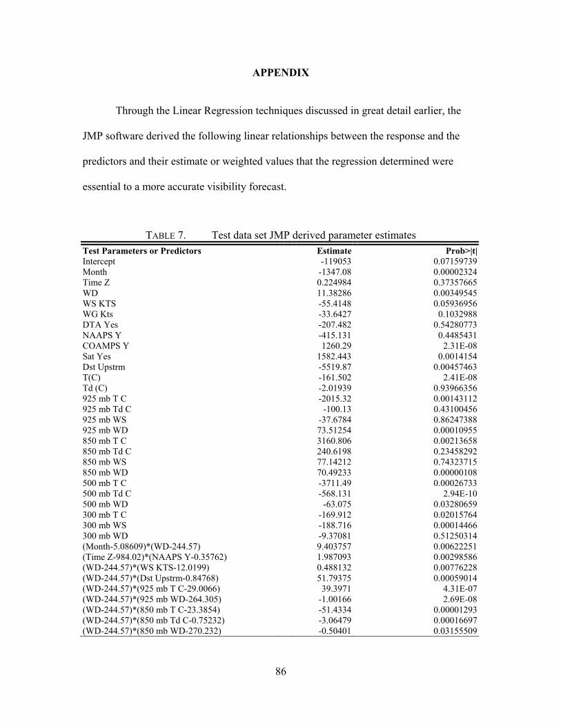
86
APPENDIX
Through the Linear Regression techniques discussed in great detail earlier, the
JMP software derived the following linear relationships between the response and the
predictors and their estimate or weighted values that the regression determined were
essential to a more accurate visibility forecast.
TABLE 7. Test data set JMP derived parameter estimates Test Parameters or Predictors Estimate Prob>|t|Intercept -119053 0.07159739Month -1347.08 0.00002324Time Z 0.224984 0.37357665WD 11.38286 0.00349545WS KTS -55.4148 0.05936956WG Kts -33.6427 0.1032988DTA Yes -207.482 0.54280773NAAPS Y -415.131 0.4485431COAMPS Y 1260.29 2.31E-08Sat Yes 1582.443 0.0014154Dst Upstrm -5519.87 0.00457463T(C) -161.502 2.41E-08Td (C) -2.01939 0.93966356925 mb T C -2015.32 0.00143112925 mb Td C -100.13 0.43100456925 mb WS -37.6784 0.86247388925 mb WD 73.51254 0.00010955850 mb T C 3160.806 0.00213658850 mb Td C 240.6198 0.23458292850 mb WS 77.14212 0.74323715850 mb WD 70.49233 0.00000108500 mb T C -3711.49 0.00026733500 mb Td C -568.131 2.94E-10500 mb WD -63.075 0.03280659300 mb T C -169.912 0.02015764300 mb WS -188.716 0.00014466300 mb WD -9.37081 0.51250314(Month-5.08609)*(WD-244.57) 9.403757 0.00622251(Time Z-984.02)*(NAAPS Y-0.35762) 1.987093 0.00298586(WD-244.57)*(WS KTS-12.0199) 0.488132 0.00776228(WD-244.57)*(Dst Upstrm-0.84768) 51.79375 0.00059014(WD-244.57)*(925 mb T C-29.0066) 39.3971 4.31E-07(WD-244.57)*(925 mb WD-264.305) -1.00166 2.69E-08(WD-244.57)*(850 mb T C-23.3854) -51.4334 0.00001293(WD-244.57)*(850 mb Td C-0.75232) -3.06479 0.00016697(WD-244.57)*(850 mb WD-270.232) -0.50401 0.03155509

87
Test Parameters or Predictors Estimate Prob>|t|(WD-244.57)*(500 mb T C+8.01523) 43.77943 0.00025333(WD-244.57)*(500 mb Td C+27.9298) 1.660285 0.03985711(WD-244.57)*(500 mb WD-246.556) 0.601492 0.00865206(WS KTS-12.0199)*(WG Kts-17.2781) -5.26107 0.00714926(WS KTS-12.0199)*(DTA Yes-0.12583) -493.006 0.00002445(WS KTS-12.0199)*(COAMPS Y-0.27152) 229.7375 0.00046302(WS KTS-12.0199)*(Dst Upstrm-0.84768) 179.2752 0.04582129(WS KTS-12.0199)*(925 mb T C-29.0066) -67.3868 0.04790503(WS KTS-12.0199)*(850 mb T C-23.3854) 57.82401 0.10682985(WS KTS-12.0199)*(500 mb Td C+27.9298) -10.6988 0.00006378(WG Kts-17.2781)*(DTA Yes-0.12583) 213.8933 0.00060494(WG Kts-17.2781)*(925 mb T C-29.0066) 113.5955 0.00036958(WG Kts-17.2781)*(925 mb Td C-3.8543) 10.91442 0.00458294(WG Kts-17.2781)*(925 mb WD-264.305) -0.75336 0.0858824(WG Kts-17.2781)*(850 mb T C-23.3854) -120.777 0.00048916(WG Kts-17.2781)*(850 mb WS-22.2985) -4.06543 0.05341369300 mb Td C 229.7776 0.03769635Alstg 2309.713 0.29746336
TABLE 8. Validation data set JMP derived parameter estimates Validation Parameter or Predictors Estimate Prob>|t|Intercept 298977.385 0.011747Month 18.4557721 0.983557Time Z 0.54673813 0.161324WD 10.4913999 0.169023WS KTS 13.2303792 0.758333WG Kts -104.6832 0.00825DTA Yes -3483.8447 0.051086NAAPS Y -137.36293 0.767593COAMPS Y 528.015307 0.233155Sat Yes 1361.61807 0.102472Dst Upstrm -2727.1432 0.045528T(C) -34.924235 0.55191Td (C) -41.695016 0.45868925 mb T C -885.79588 0.074236925 mb Td C -472.05759 0.008309925 mb WS 338.997643 0.001264925 mb WD -9.6283126 0.078877850 mb T C 1129.74663 0.157707850 mb Td C 843.593251 1.96E-05850 mb WS 56.2956598 0.409648850 mb WD -20.197711 0.091346500 mb T C -782.72622 0.073033500 mb Td C -173.65196 0.021423500 mb WD 17.5489884 0.15661300 mb T C -3.3112611 0.913284300 mb WS 24.5292432 0.497193300 mb WD -22.016338 0.155694(Month-5.25547)*(WD-269.343) -15.084072 0.093607(Month-5.25547)*(Dst Upstrm-0.65693) -1744.0708 0.000441

88
Validation Parameter or Predictors Estimate Prob>|t|(Time Z-969.109)*(NAAPS Y-0.40146) 2.15676417 0.006249(WD-269.343)*(WS KTS-14.5839) 0.51025042 0.193222(WD-269.343)*(Dst Upstrm-0.65693) -23.513513 0.057295(WD-269.343)*(925 mb T C-28.2073) 21.9980922 2.61E-05(WD-269.343)*(925 mb WD-262.372) 0.08227234 0.061733(WD-269.343)*(850 mb T C-24.1898) -30.600183 7.73E-05(WD-269.343)*(850 mb Td C+1.10365) 0.4394088 0.787704(WD-269.343)*(850 mb WD-297.08) 0.10576304 0.100353(WD-269.343)*(500 mb T C+7.43796) 12.478342 0.040998(WD-269.343)*(500 mb WD-245.474) -0.0182657 0.923577(WS KTS-14.5839)*(WG Kts-21.4307) 0.09700078 0.973355(WS KTS-14.5839)*(DTA Yes-0.11679) -297.80019 0.118819(WS KTS-14.5839)*(COAMPS Y-0.28467) -76.454577 0.332701(WS KTS-14.5839)*(Dst Upstrm-0.65693) -87.381885 0.459338(WS KTS-14.5839)*(925 mb T C-28.2073) 55.5830179 0.071807(WS KTS-14.5839)*(850 mb T C-24.1898) -58.88157 0.15336(WS KTS-14.5839)*(500 mb Td C+30.8372) -8.1098237 0.004785(WG Kts-21.4307)*(925 mb T C-28.2073) -46.455087 0.025855(WG Kts-21.4307)*(925 mb WD-262.372) -0.672593 0.012046(WG Kts-21.4307)*(850 mb T C-24.1898) 56.9208504 0.054555(WG Kts-21.4307)*(850 mb WS-17.9565) -1.5620222 0.509202(WG Kts-21.4307)*(925 mb Td C-3.43723) 0.91824853 0.766801Alstg -10950.536 0.004634300 mb Td C -430.76673 0.001361(WG Kts-21.4307)*(DTA Yes-0.11679) 95.7738632 0.4343

89
Bibliography
Air Force Combat Climatology Center, 1957: Forecasting Visibility Restrictions Due to Dust at Dhahran Air Base in Summer, AD-161712, 4 pp.
Air Force Combat Climatology Center, 1970: Iraq and Arabian Peninsula climate and weather, NIS 30 and 32, 92 pp. Air Force Manual (AFMAN) 15-111, Surface Weather Observations, 18 September
2001. Air University Style Guide for Writers and Editors, Maxwell AFB, AL.: Air University Press, 2001, 137 pp. American Meteorological Society, 2002: A Brief Guide for Authors. American
Meteorological Society, Boston, MA Barnum, B. H., N. S. Winstead, L. J. Wesley, A. Hokola, P. Colarco, O. B. Toon, P. Ginoux, G. W. Brooks, L. Hasselbarth and B. Toth, 2003: Forecasting dust storms using CARMA-dust model and MM5 weather data, [On-line at https://weather.afwa.af.mil/about_info/DTA/DTA_Tutorial.html], 16 pp. Bukhari, S. A., 1993: Depicting dust and sand storm signatures through the means of satellite images and ground-based observations for Saudi Arabia, University of Colorado, Boulder, CO, 130 pp. Clements, T., J. F. Mann Jr., R. O. Stone, and J. A. Eymann, 1963: A study of windborne sand and dust in desert areas, U. S. Army Tech. Rep. ES-8, 61 pp. Fleet Numerical METOC Detachment (FNMOD) NOGAPS Climatology, 2003: Fleet
Numerical Meteorology and Oceanography Detachment, Asheville, NC. [On-line at http://navy.ncdc.noaa.gov/gradsmap/indexcustomfhf.html]
Fujita, T. T., 1984: Andrews AFB microburst, SMRP Res. Paper 205, University of Chicago, IL, 38 pp. Glickman, T. S., 2000: Glossary of Meteorology, 2nd Ed., American Meteorological Society, 855 pp. Global Security, 2003: Global Security.Org, Alexandria, VA. [On-line at
http://www.globalsecurity.org/military/facility/udeid.htm]

90
Idso, S. B., R. S. Ingram, and J. M. Pritchard, 1972: An American haboob, Bulletin of the American Meteorological Society, 53, 930-935. Lewis, L. J., and P. J. Feteris, 1989: Diagnostic study of atmospheric-terrain interaction
leading to the formation of dust clouds and poor visibilities over near east desert areas, Department of Physics and Atmospheric Sciences, Jackson State University, Jackson, MS, 20 pp.
Liu, M., Walker, A. L., Westphal D. L., and Richardson, K., Dust Forecasting for Operation Iraqi Freedom, 2003: Naval Research Laboratory, Monterey, CA. [On-line at http://www.nrlmry.navy.mil/aerosol/index_frame.html]
Membery, D. A., 1983: Low level wind profiles during the Gulf Shamal, Weather, 38, 18-24. Membery, D. A., 1985: Gravity wave haboob, Weather, 40, 214-221. Miller, S. D., Hawkins, J., Turk, J., Lee, T., Richardson, K., and Kuciauskas, A.,
2003: Satellite Focus: A Dynamic, Near Real-Time Satellite Resource for the DoD, The Battlespace Atmospheric and Cloud Impacts on Military Operations (BACIMO) Conference, 9-11 September 2003, Monterey, CA.
Miller, S. D., 2003: Satellite Surveillance of Desert Dust Storms, NRL Review, 69-77 Miner, T., 2003: Sand, dust and ash: The answer is blowing in the wind, United States Air Force Flying Safety Magazine, May, 4-7. Mireless, M., Pederson, K., Elford, C., Reyman, M., Piasecki, J., Hosein F., Larabee, S.,
Williams, G., Jimenez, M., and Chapdelaine, D., 2002: Meteorological Techniques, AFWA/TN—98/002, Air Force Weather Agency, 285 pp.
Montgomery, D. C., and G. C. Runger, 2003: Applied Statistics and Probability For
Engineers, 3rd Ed., John Wiley and Sons, Inc., New York, NY, 706 pp. Naval Research Lab (NRL), Monterey Aerosol Page, 2003: Marine Meteorology Division, Monterey, CA. [On-line at http://www.nrlmry.navy.mil/aerosol/index_frame.html] Neter, J., Wasserman, W., and Kutner, M. H., 1990: Applied Linear Statistical Models
Regression, Analysis of Variance, and Experimental Designs, 3rd Ed., Homewood, IL., Irwin, 1181 pp.
Perrone, T. J., 1979: Winter Shamal in the Persian Gulf, Naval Environmental Prediction Research Facility, TR 79-06, 168 pp.

91
Prospero, J. M., D. M. Helgren, J. Fernandez-Partagas, and M. Estoque, 1986: Environmental conditions associated with the occurrence of large scale dust storms in arid regions of North Africa, University of Miami, Rosenthal School of Marine and Atmospheric Science, Miami, FL, 19 pp.
Rao, P. G., M. Al-Sulaiti, and A. H. Al-Mulla, 2001: Winter shamals in Qatar, Arabian Gulf, Weather, 56, 444-451
Safar, M. I., 1980: Dust and duststorms in Kuwait, State of Kuwait Directorate General of Civil Aviation, Meteorological Dept., Climatological Section, 137 pp. Salford Systems, 1995: Data Mining with Decision Trees: An Introduction to CART®.
San Diego, CA, 133 pp. Salford Systems, 2002: CART® for Windows User’s Guide. San Diego, CA, 295 pp. SAS Institute, 2003: JMP Users Guide. Cary, N.C. [On-line at
http://web.utk.edu/~leon/jmp/default.html] “Satellite Focus”, Naval Research Lab (NRL), 2003: Marine Meteorology Division, Monterey, CA. [On-line at http://www.nrlmry.navy.mil/focus-bin/focus.cgi] Siraj, A. A., 1980: Aziab weather, General Directorate of Meteorology, Saudi Arabia, 22 pp. Wigner, K. A., and R. E. Peterson, 1982: Duststorms over Texas. Preprints, 2nd
Symposium on the Composition of the Non-Urban Troposphere, Williamsburg, VA, 52-71.
Wilkerson, W. D., 1991: Dust and sand forecasting in Iraq and adjoining countries, AWS/TN—91/001, Air Weather Service, Scott AFB, IL, 63 pp. Wilks, D.S., 1995: Statistical Methods in the Atmospheric Sciences, Academic Press, San
Diego, CA, 467 pp.

92
REPORT DOCUMENTATION PAGE Form Approved OMB No. 074-0188
The public reporting burden for this collection of information is estimated to average 1 hour per response, including the time for reviewing instructions, searching existing data sources, gathering and maintaining the data needed, and completing and reviewing the collection of information. Send comments regarding this burden estimate or any other aspect of the collection of information, including suggestions for reducing this burden to Department of Defense, Washington Headquarters Services, Directorate for Information Operations and Reports (0704-0188), 1215 Jefferson Davis Highway, Suite 1204, Arlington, VA 22202-4302. Respondents should be aware that notwithstanding any other provision of law, no person shall be subject to an penalty for failing to comply with a collection of information if it does not display a currently valid OMB control number. PLEASE DO NOT RETURN YOUR FORM TO THE ABOVE ADDRESS. 1. REPORT DATE (DD-MM-YYYY)
March 2004 2. REPORT TYPE
Master’s Thesis
3. DATES COVERED (From – To) Jun 2003 – Mar 2004
5a. CONTRACT NUMBER 5b. GRANT NUMBER
4. TITLE AND SUBTITLE DUST STORM FORECASTING FOR AL UDEID AB, QATAR: AN EMPIRICAL ANALYSIS 5c. PROGRAM ELEMENT NUMBER
5d. PROJECT NUMBER None 5e. TASK NUMBER
6. AUTHOR(S) Bartlett, Kevin S., Captain, USAF 5f. WORK UNIT NUMBER 7. PERFORMING ORGANIZATION NAMES(S) AND ADDRESS(S) Air Force Institute of Technology Graduate School of Engineering and Physics (AFIT/ENP) 2950 P Street, Building 640 WPAFB OH 45433-7765
8. PERFORMING ORGANIZATION REPORT NUMBER AFIT/GM/ENP/04-01
10. SPONSOR/MONITOR’S ACRONYM(S)
9. SPONSORING/MONITORING AGENCY NAME(S) AND ADDRESS(ES) Chief, Tactical Capabilities Development Attn: Capt Gerald Sullivan HQ Air Combat Command/Weather Operations Division (HQ ACC/DOW) 205 Dodd Blvd, Ste 101 DSN: 574-8442 Langley AFB, VA 23665-2789 e-mail:[email protected]
11. SPONSOR/MONITOR’S REPORT NUMBER(S)
12. DISTRIBUTION/AVAILABILITY STATEMENT APPROVED FOR PUBLIC RELEASE; DISTRIBUTION UNLIMITED.
13. SUPPLEMENTARY NOTES 14. ABSTRACT Dust storms are extreme weather events that have strong winds laden with visibility reducing and operations limiting dust. The Central Command Air Forces (CENTAF) 28th Operational Weather Squadron (OWS) is ultimately responsible for forecasting weather in the vast, data denied region of Southwest Asia in support of daily military and humanitarian operations. As a result, the 28th OWS requests a simplified forecasting tool to help predict mesoscale dust events that affect coalition operations at Al Udeid AB, Qatar. This research satisfies the 28th OWS request through an extensive statistical analysis of observational data depicting seasonal dust events over the past 2 years. The resultant multiple linear regression best fit model combines 28 easily attainable model outputs, satellite imagery, surface and upper air observations, and applies a linear transformation equation. The model provides the end user with a numerical visibility prediction for Al Udeid AB that is verified against a seasonally divided and independent validation data set that yields an R2 of 0.79 while maintaining < 800 m accuracy. The operational significance of the summarized seasonal patterns and dust storm type offers operators within the region a quick synopsis of possible dust prone periods and duration of events; whereas the best Fit Model offers an easy-to-use, accurate dust forecasting tool. The Fit Model developed is ready to use and is expected to positively affect weather forecasts for flight operations at Al Udeid AB.
15. SUBJECT TERMS Dust storms, dust storm forecasting, Qatar weather, Al Udeid AB weather, Persian Gulf weather 16. SECURITY CLASSIFICATION OF:
19a. NAME OF RESPONSIBLE PERSON Steven T. Fiorino, Maj USAF (ENP)
a. REPORT
U
b. ABSTRACT
U
c. THIS PAGE
U
17. LIMITATION OF ABSTRACT
UU
18. NUMBER OF PAGES
103 19b. TELEPHONE NUMBER (Include area code) (937) 255-3636 x4506 e-mail: [email protected]
Standard Form 298 (Rev. 8-98) Prescribed by ANSI Std. Z39-18