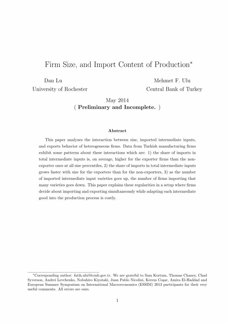
Firm Size, and Import Content of Production∗

Dan Lu Mehmet F. Ulu

University of Rochester Central Bank of Turkey

May 2014( Preliminary and Incomplete. )

Abstract

This paper analyzes the interaction between size, imported intermediate inputs,

and exports behavior of heterogeneous firms. Data from Turkish manufacturing firms

exhibit some patterns about these interactions which are: 1) the share of imports in

total intermediate inputs is, on average, higher for the exporter firms than the non-

exporter ones at all size percentiles, 2) the share of imports in total intermediate inputs

grows faster with size for the exporters than for the non-exporters, 3) as the number

of imported intermediate input varieties goes up, the number of firms importing that

many varieties goes down. This paper explains these regularities in a setup where firms

decide about importing and exporting simultaneously while adapting each intermediate

good into the production process is costly.

∗Corresponding author: fatih.ulu@tcmb.gov.tr. We are grateful to Sam Kortum, Thomas Chaney, ChadSyverson, Andrei Levchenko, Nobuhiro Kiyotaki, Juan Pablo Nicolini, Kerem Cosar, Amira El-Haddad andEuropean Summer Symposium on International Macroeconomics (ESSIM) 2013 participants for their veryuseful comments. All errors are ours.

1

1 Introduction

One of the common patterns for countries that reduce their trade barriers is the surge in

their exports accompanied with an even bigger increase in their imports. At the same time,

import content of exports increases in these countries.1 We also know that two thirds of world

trade is in intermediate goods (Hummels et al. (2001)). Beside these, when a production

function with three production factors -labor,capital and intermediate goods- is estimated for

industries, the biggest share of the total cost of production is spent for intermediate goods.2

These findings combined suggest that intermediate goods are important in both trade and

production processes, and this study analyzes the joint role of intermediate goods in trade

and production processes, which has not been explored completely yet.

This paper analyzes the interaction between firm productivity, imported intermediate

inputs, and exports behavior of firms. It explains the regularities observed in the data about

these interactions in a setup where after receiving their productivity and demand shocks

firms decide about importing and exporting simultaneously while adapting each imported

intermediate good into the production process is costly and costs grow convexly in the

number of imported varieties.

Different aspects of the fragmentation of production processes across countries have been

analyzed under different names in several other studies.3,4 Next to the theoretical studies of

the topic some other studies have analyzed and quantified couple channels for the impact

of trade in intermediate goods other economic decisions of firms.5 Goldberg et al. (2010)

investigate the impact of trade barrier reductions on intermediate goods imports and con-

sequently firm product scope. They state that in the analyzed period in India, 31% of the

new products launched by domestic firms accounted for the lower tariff barriers. Availability

of new intermediate inputs which were not available prior to barrier reduction is the main

factor that drove this outcome. In Halpern et al. (2011) imported inputs affect TFP, and

they find large productivity effects of imported inputs. Kasahara and Rodrigue (2008) also

finds evidence from Chilean data that importing intermediate inputs improves productivity.

Kasahara and Lapham (2013) analyze the interaction between productivity and decisions to

1Trade barrier reductions between EU and Central and Eastern European countries may give us examplesof these situations.

2In Amiti and Konings (2007) for almost all manufacturing sectors the share of intermediate goods intotal production costs is between 60% and 70%.

3Some of these names are offshoring, outsourcing, global value chains, global production chains, fragmen-tation of production.

4Grossman and Rossi-Hansberg (2008) has a good list of related references.5Grossman and Rossi-Hansberg (2008) propose a theory of global production processes with tradeable

tasks, and analyze the impact changes in offshoring costs on domestic factor prices. Costinot et al. (forth-coming) offer a perspective on how vertical specialization shapes the interdependence of nations.

2

import and export. They develop a theoretical model and estimate their structural model

empirically. Johnson and Noguera (2012) find that variation in aggregate VAX (value added

to exports) ratios across countries is, to a large extent, driven by variation in the composition

of exports. Bergin et al. (2009) show how global production sharing affects the volatility of

economic activity. Feenstra and Hanson (1997) indicate that outsourcing explains significant

fractions of the increase in the relative wages of non-production workers at industry level.

As to the motives behind firms’ import behaviors, a recent study by Saygl et al. (2010)

presents results of their interviews with the big intermediate input importers in Turkey.

These interviewed firms produce 35.9% of total manufacturing value added and export 24.8%

of manufactured goods. 96.6% of these firms mention lack of domestic supply of the imported

input, and 75.2% of them also mention purchasing more quality inputs for cheaper from

abroad as their motives for importing. Firms’ responses in these interviews also justify our

approach which accounts for quality differences between the imported intermediates and the

domestic ones.

The mechanism that we propose to explain the interaction between intermediate goods,

productivity and the value added content of exports builds on the the approach of Gopinath

and Neiman (2014) for modelling the decision of firm about how much imported intermediate

input to employ in production. We augment their model by introducing an exports market

which is costly to enter (e.g., Melitz (2003)). Firms have incentive to use more imported

intermediate inputs due to the quality of intermediate input that can be embedded to the

productivity of the firm as well as the love-of-variety in the production technologies.

Halpern et al. (2011) have an idea similar to ours. However, they do not analyze the

interaction between firm size, input imports and export behavior of firms which we focus on.

Our model diverges from Kasahara and Lapham (2013) in several respects. First, in their

set up imported inputs increase productivity only through the channel of love-of-variety in

the production function. Instead, we introduce quality differences into intermediate inputs,

and these quality differences across intermediate inputs directly affect the productivity of

firms. A second difference of our work is that we explicitly model firms’ decisions about the

number of different varieties to import. This aspect of our model provides an explanation

for the fact that is observed in the data that the gap between average intermediate import

ratios for exporters and non-exporters grows with the firm size.

Since the marginal productivity gains through importing one more good will be higher

for them, more productive firms will be more willing to import more varieties of intermediate

inputs. On the other side, the fixed cost of importing will be convex in the number of different

varieties imported. Hence, for each firm with an initial productivity, there will be an optimal

number of different varieties to be imported. This situation gives more productive firms more

3

room to improve their productivities by importing a more diverse set of intermediate inputs.

It is already established in the previous studies that only sufficiently productive firms enter

the export markets in the existence of fixed entry costs. Imported intermediate goods give

the more productive firms the ability to become even more productive relative to the less

productive firms. More productive firms import more, become even more productive, and

hence export even more, and their exported goods are on average more import intensive.

For calibrating the model we target a list of moments that includes the intermediate

import ratios of exporter and non-exporter firms at all sizes, and the distribution of the

number of imported intermediate inputs. Findings from the calibration gives estimates for

the deep parameters that govern the interaction between firm productivity and firms’ import

and export decisions, and allow me to have some counterfactual experiments.

2 Data and Facts

We combine two distinct datasets from the Turkish Statistical Institute (TurkStat), which

are the trade transactions and structural business datasets for Turkish firms. We focus our

analysis on only the manufacturing firms (NACE 15-37) in 2008. We observe both import

and export numbers as well as some balance sheet items of these firms. In this section, we

present some regularities about firm size, number of imported varieties, expenditure share

of imported intermediate inputs in total intermediate input expenditure and firms’ importer

and exporter statuses.

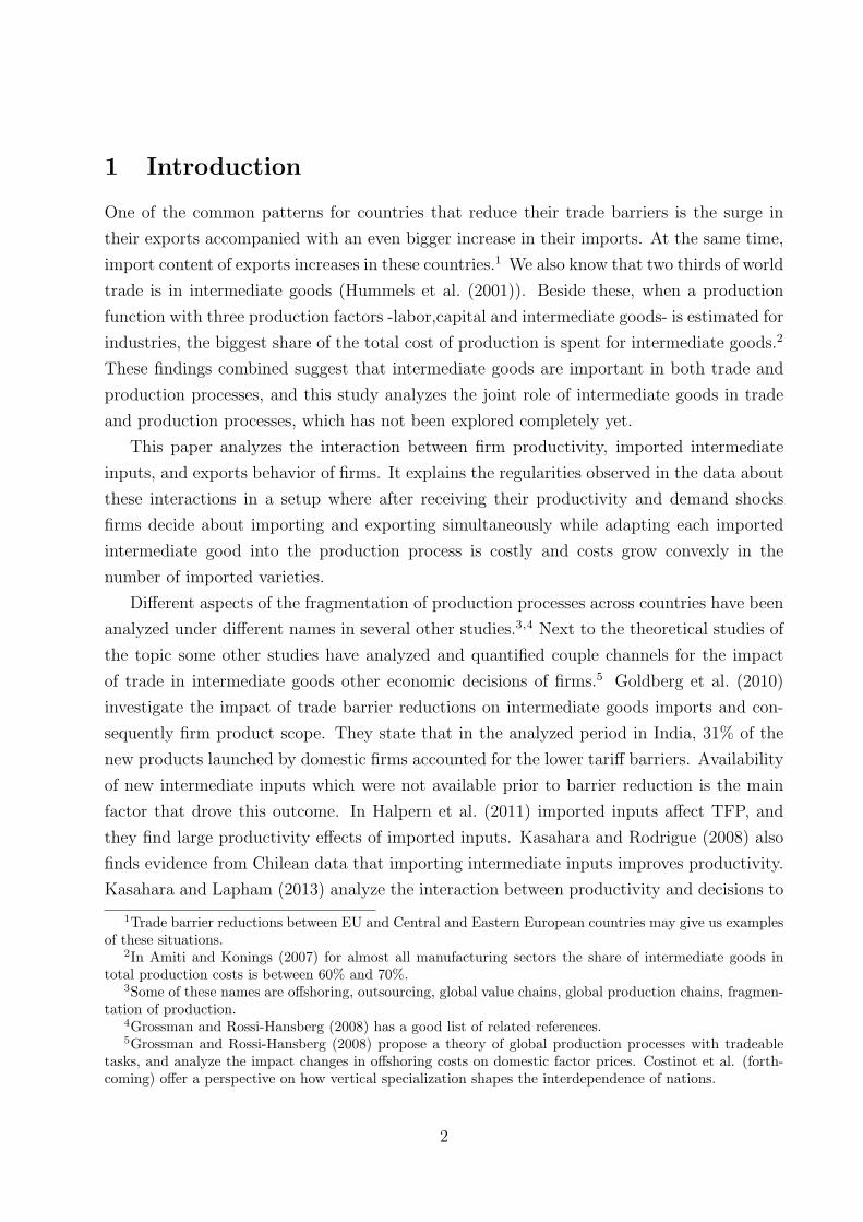
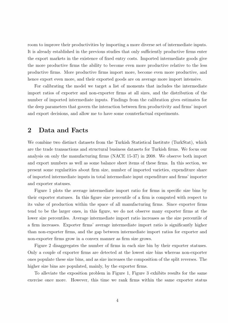
Figure 1 plots the average intermediate import ratio for firms in specific size bins by

their exporter statuses. In this figure size percentile of a firm is computed with respect to

its value of production within the space of all manufacturing firms. Since exporter firms

tend to be the larger ones, in this figure, we do not observe many exporter firms at the

lower size percentiles. Average intermediate import ratio increases as the size percentile of

a firm increases. Exporter firms’ average intermediate import ratio is significantly higher

than non-exporter firms, and the gap between intermediate import ratios for exporter and

non-exporter firms grow in a convex manner as firm size grows.

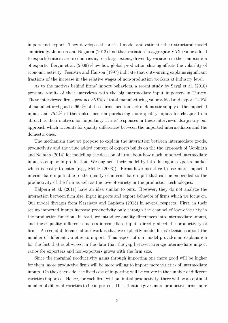
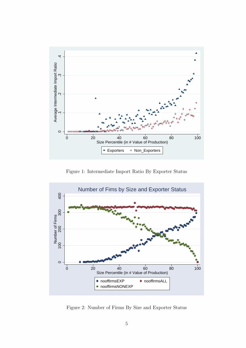
Figure 2 disaggregates the number of firms in each size bin by their exporter statuses.

Only a couple of exporter firms are detected at the lowest size bins whereas non-exporter

ones populate these size bins, and as size increases the composition of the split reverses. The

higher size bins are populated, mainly, by the exporter firms.

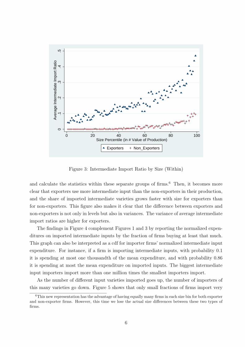
To alleviate the exposition problem in Figure 1, Figure 3 exhibits results for the same

exercise once more. However, this time we rank firms within the same exporter status

4

0.1

.2.3

.4A

vera

ge In

term

edia

te Im

port

Rat

io

0 20 40 60 80 100Size Percentile (in # Value of Production)

Exporters Non_Exporters

Figure 1: Intermediate Import Ratio By Exporter Status

010

020

030

040

0N

umbe

r of

Firm

s

0 20 40 60 80 100Size Percentile (in # Value of Production)

nooffirmsEXP nooffirmsALLnooffirmsNONEXP

Number of Fims by Size and Exporter Status

Figure 2: Number of Firms By Size and Exporter Status

5

0.1

.2.3

.4.5

Ave

rage

Inte

rmed

iate

Impo

rt R

atio

0 20 40 60 80 100Size Percentile (in # Value of Production)

Exporters Non_Exporters

Figure 3: Intermediate Import Ratio by Size (Within)

and calculate the statistics within these separate groups of firms.6 Then, it becomes more

clear that exporters use more intermediate input than the non-exporters in their production,

and the share of imported intermediate varieties grows faster with size for exporters than

for non-exporters. This figure also makes it clear that the difference between exporters and

non-exporters is not only in levels but also in variances. The variance of average intermediate

import ratios are higher for exporters.

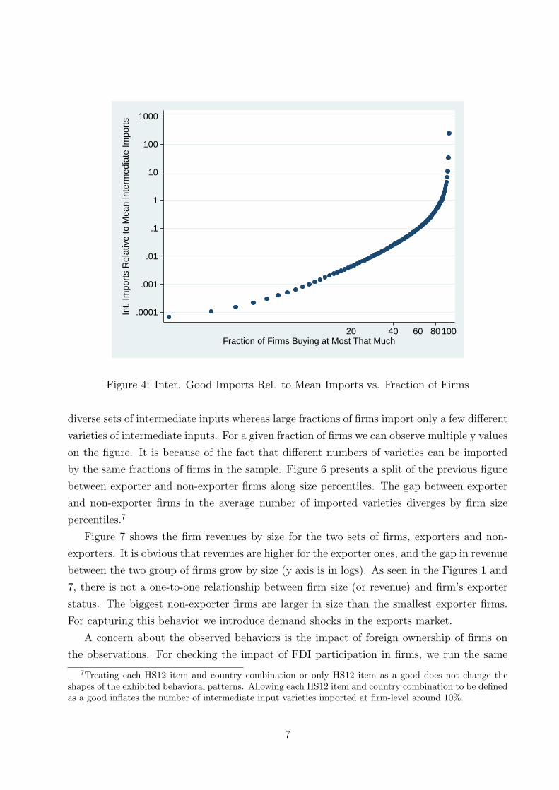
The findings in Figure 4 complement Figures 1 and 3 by reporting the normalized expen-

ditures on imported intermediate inputs by the fraction of firms buying at least that much.

This graph can also be interpreted as a cdf for importer firms’ normalized intermediate input

expenditure. For instance, if a firm is importing intermediate inputs, with probability 0.1

it is spending at most one thousandth of the mean expenditure, and with probability 0.86

it is spending at most the mean expenditure on imported inputs. The biggest intermediate

input importers import more than one million times the smallest importers import.

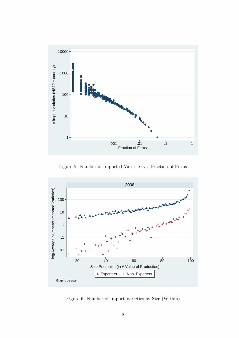
As the number of different input varieties imported goes up, the number of importers of

this many varieties go down. Figure 5 shows that only small fractions of firms import very

6This new representation has the advantage of having equally many firms in each size bin for both exporterand non-exporter firms. However, this time we lose the actual size differences between these two types offirms.

6

.0001

.001

.01

.1

1

10

100

1000In

t. Im

port

s R

elat

ive

to M

ean

Inte

rmed

iate

Impo

rts

20 40 60 80100Fraction of Firms Buying at Most That Much

Figure 4: Inter. Good Imports Rel. to Mean Imports vs. Fraction of Firms

diverse sets of intermediate inputs whereas large fractions of firms import only a few different

varieties of intermediate inputs. For a given fraction of firms we can observe multiple y values

on the figure. It is because of the fact that different numbers of varieties can be imported

by the same fractions of firms in the sample. Figure 6 presents a split of the previous figure

between exporter and non-exporter firms along size percentiles. The gap between exporter

and non-exporter firms in the average number of imported varieties diverges by firm size

percentiles.7

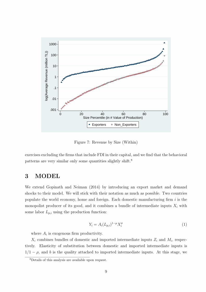
Figure 7 shows the firm revenues by size for the two sets of firms, exporters and non-

exporters. It is obvious that revenues are higher for the exporter ones, and the gap in revenue

between the two group of firms grow by size (y axis is in logs). As seen in the Figures 1 and

7, there is not a one-to-one relationship between firm size (or revenue) and firm’s exporter

status. The biggest non-exporter firms are larger in size than the smallest exporter firms.

For capturing this behavior we introduce demand shocks in the exports market.

A concern about the observed behaviors is the impact of foreign ownership of firms on

the observations. For checking the impact of FDI participation in firms, we run the same

7Treating each HS12 item and country combination or only HS12 item as a good does not change theshapes of the exhibited behavioral patterns. Allowing each HS12 item and country combination to be definedas a good inflates the number of intermediate input varieties imported at firm-level around 10%.

7

1

10

100

1000

10000#

impo

rt v

arie

ties

(HS

12 −

cou

ntry

)

.001 .01 .1 1Fraction of Firms

Figure 5: Number of Imported Varieties vs. Fraction of Firms

.01

.1

1

10

100

20 40 60 80 100

2008

Exporters Non_Exporters

log(

Ave

rage

Num

bero

f Im

port

ed V

arie

ties)

Size Percentile (in # Value of Production)

Graphs by year

Figure 6: Number of Import Varieties by Size (Within)

8

.001

.01

.1

1

10

100

1000lo

g(A

vera

ge R

even

ue (

mill

ion

TL)

)

0 20 40 60 80 100Size Percentile (in # Value of Production)

Exporters Non_Exporters

Figure 7: Revenue by Size (Within)

exercises excluding the firms that include FDI in their capital, and we find that the behavioral

patterns are very similar only some quantities slightly shift.8

3 MODEL

We extend Gopinath and Neiman (2014) by introducing an export market and demand

shocks to their model. We will stick with their notation as much as possible. Two countries

populate the world economy, home and foreign. Each domestic manufacturing firm i is the

monopolist producer of its good, and it combines a bundle of intermediate inputs Xi with

some labor Lp,i using the production function:

Yi = Ai(Lp,i)1−µXµ

i (1)

where Ai is exogenous firm productivity.

Xi combines bundles of domestic and imported intermediate inputs Zi and Mi, respec-

tively. Elasticity of substitution between domestic and imported intermediate inputs is

1/1 − ρ, and b is the quality attached to imported intermediate inputs. At this stage, we

8Details of this analysis are available upon request.

9

assume b to be same for all imported varieties. Intermediate goods are produced by monop-

olistic producers in both the domestic and foreign markets.

Xi = [Zρi +Mρ

i ]1

ρ (2)

where

Zi =

[∫

zθijdj

] 1

θ

(3)

Mi =

[∫

Ωi

(bmik)θdk

] 1

θ

Firm i can sell its products in both domestic and foreign markets. gi is the domestic

sales while g∗i is the exports.

Yi = gi + g∗i (4)

There are three kinds of fixed costs in the environment. These costs are paid in terms

of labor units. The first kind is the fixed entry cost to be paid while entering the foreign

market, fe. The remaining two fixed costs are related to importing intermediate goods. fI

is the fixed part of import costs while fυ multiplies the part that varies with the number of

varieties imported.9,10 |Ωi| is the cardinality of the set of varieties imported by firm i. λ > 1.

governs the curvature of the variable cost of importing.11

F (|Ωi|, g∗i ) = [fII|Ωi|6=0 + fυ|Ωi|

λ + feI|g∗i |>0] (5)

Since each firm will import different sets of intermediate goods, the ideal price index

of intermediate inputs PXimay differ for each firm. PMi

is the price index for imported

intermediate inputs, will differ across firms depending on the number of varieties that firms

import |Ωi|. PZ is the equilibrium price index for domestic intermediate goods. For now, we

will treat it as exogenous and same for every firm.12 Price of each imported intermediate

input is pm, and they have the same quality b > 1 attached to them.

9For starting to import firms need to bear costs of hiring new personnel, learning the legal requirements,and other red tape costs.

10Adaptation of new imported intermediate inputs to the production process is costly. New machinery orhuman resources may be necessary for this adaptation, and fυ captures these costs.

11These convex adjustment costs allow us to capture the decreasing number of importer firms in thenumber of varieties imported, and also the convexly increasing average intermediate import ratios by firmsize.

12Allowing PZ to be endogenously determined will definitely add new insights to the model, and in futurethe model can be extended to that direction.

10

PXi=

(

Pρ

ρ−1

Z + Pρ

ρ−1

Mi

) ρ−1

ρ

if firm i imports

PZ if firm i does not import(6)

PMi=

[∫

k∈Ωi

(pmb)

θθ−1dk

] θ−1

θ

(7)

=pmb|Ωi|

θ−1

θ

where 0 < θ < 1.

The love-of-variety in the production technology brings about the inverse relationship

between between the ideal price index imported intermediate imputs PMiand the the number

of different varieties imported Ωi.In fact this relationship is a mirror image of the increasing

returns to more varieties embedded into the production process as observed in Eq. (3). This

inverse relationship is at the core of the model while explaining the observed firm behavior.

3.1 Firm’s Problem

Firm has to decide about being an exporter and an importer. If it decides to be an importer,

it also has to determine the number of varieties to import.13

Unit cost of production for firm i is Ci =1

µµ(1−µ)1−µ

w1−µPµXi

Ai.

mi =

(pmPMi

) 1

θ−1

(PMi

PXi

) 1

ρ−1

Xi if firm i imports

0 if firm i does not import(8)

Firm i receives demand shock si in the foreign market. Aside from the demand shocks,

demand and market structures in the foreign market are as they are in the domestic market.14

g∗i (si, pi) =

sip1

ε−1

i if firm i exports

0 if firm i does not export(9)

Sending goods to the foreign market is costly. For delivering one unit of product to the

foreign country τ units of good should be shipped from the home country. The price that

13In the model we have assumed the imported intermediate varieties to be a continuum, and hence, a firmcould decide about its optimal number of varieties to import by continuously differentiating their objectivefunctions. However, for mapping those decisions to the observed physical decisions of firms we have todiscretize the varieties, and in the calculations we achieve it by rounding the optimal choices of the firms.

14However, market sizes differ. Since we will analyze model in a partial equilibrium environment, we areonly interested in the parameters of the distribution from where the demand shocks come.

11

firm i charges on its products is pi and p∗i in domestic and foreign markets, respectively:

pi =Ci

ε, p∗i = τ

Ci

ε(10)

If we allow p∗i to be the price in the foreign market, then firm i’s profit from the domestic

and foreign markets are πi = (pi − Ci)p1

ε−1

i = (1 − ε)(pi)ε

ε−1

and π∗i = si(1 − ε)(p∗i )

εε−1

,

respectively. Πi = πi + π∗i is the gross profit from both markets.

(Ωi, gi, g∗i ) = arg max

Ωi,gi,g∗

i

πi = (1− ε)Ri − wF (|Ωi|, g∗i ) (11)

The firm determines its PMi, and hence PXi

and consequently the unit cost of production

Ci by deciding about the optimal number of varieties to import. The firm’s action set about

importing and exporting is comprised of four possible actions: neither import nor export,

only import, only export, and both import and export. For each action, the optimal number

of varieties to import may differ, and the firm maximizes profit by picking one of these

actions.

After observing its productivity and demand shocks A and s, a firm decides about whether

to be an exporter and how much intermediates to import simultaneously. A firm’s exporter

status and the number of varieties that the firm imports are positively correlated. A firm

earns directly and indirectly from exporting goods. The direct return to the firm from

entering into the foreign market is selling its goods in this new market with a markup. The

indirect return is through importing more varieties. Since it is selling its goods in a larger

market, any effort to reduce unit production costs pays more to the firm. That’s why, the

firm will be more eager to employ more imported varieties in production, and consequently

lower its unit production costs.

As the unit cost of production increases, profits go down, and unit cost of production

comoves with factor prices, w and PX . Even if there is no quality difference between the

domestic and imported intermediate goods, more imported varieties decreases the unit costs

of production because of the love-of-variety in the production technology. If a quality that

is higher than the quality of the domestic intermediates is attached to the imported inter-

mediates -b > 1- than the cost reducing impact of imported intermediates becomes stronger.

Ri = W [p(Ωi)ε

ε−1 + I(g∗ > 0)sip∗(Ωi)

εε−1 ] (12)

W is the market size parameter. It multiplies the demands in both home and foreign

markets, and acts as a demand shifter.

Firm’s FOC regarding Ω is

12

∂π

∂Ω= W (1− ε)(1 + I(g∗ > 0)sτ

εε−1 )

∂p(Ω)ε

ε−1

∂Ω− λwfνΩ

λ−1 = 0 (13)

=⇒ κµε

ε− 1

θ − 1

θ

(pmb

) ρρ−1

Pµεε−1

+ ρ1−ρ

X = λwfνΩλ− θ−1

θρ

ρ−1

where κ = W (1 − ε)(1 + I(g∗ > 0)sτε

ε−1 )εε

1−ε

(w1−µ

Aµµ(1−µ)1−µ

) εε−1

. By deciding Ωi in fact

each firm decides about the price of intermediate inputs bundle PXithat they will face

and hence the unit cost of production Ci that they will incur. λwfνΩλ− θ−1

θρ

ρ−1 represents

the marginal cost of increasing the number of imported varieties and adding them to the

production process. This marginal cost definitely increases with convexity of the adjustment

cost function, and λ governs convexity of this cost function. The exponent term λ− θ−1θ

ρ

ρ−1

exhibits that as the θ goes down which means that elasticity of substitution among imported

varieties increases the marginal cost of adapting one more variety. As ρ goes down and hence

the elasticity of substitution between the domestic and imported intermediate varieties goes

up again marginal cost of adapting imported varieties goes down. The right-hand side of 13

exhibit returns to increasing number of imported varieties embedded to production process.

It mainly reduces PX and this effect is amplifies by the exponent µε

ε−1+ ρ

1−ρ. µ is the cost

share of the bundle intermediate inputs in production and marginal returns to importing

more varieties is deepened with this cost share as well as the elasticity of demand. More

elastic the demand more returns to any decline in unit production costs. Adversely, as ρ goes

up the domestic and imported intermediate inputs become more substitutable and hence the

unit production cost reducing impact of importing more varieties is lessened.

3.2 Discussions

The expenditure share of import in total intermediate inputs used (IIS) increases with the

price of domestically supplied intermediate inputs and decreases with the price of imported

inputs. The elasticity of IIS with respect to the optimal number of imported varieties isθ−1θ

ρ

ρ−1. Since domestic and imported inputs are not perfect substitutes, as θ goes up (hence,

the within elasticity of substitution for each type of intermediate inputs) the impact of this

change through Ω reduces the IIS. For the same number of imported varieties, the firm will

demand more domestic inputs and consequently the expenditure share of imported inputs

will increase. For the same number of imported varieties when the elasticity of substitution

between imported and domestically produced goods ρ increases, the cost share of imported

inputs goes down.

13

Em

EZ

=(pm)

ρρ−1 (b)

1

θ−1− 1

ρ−1

(PZ)ρ

ρ−1

Ωθ−1

θρ

ρ−1 (14)

∂(Em/EZ)

∂Ω> 0,

∂(Em/EZ)

∂pm< 0,

∂(Em/EZ)

∂PZ

> 0 (15)

The elasticity of the cost share of imported inputs with respect to firm size is governed

by the elasticity of substitution among goods of the same origin (θ), across goods of different

origins (ρ) and the elasticity of the optimal number of imported varieties with respect to

firm size.

∂ln(Em/EZ)

∂lnY=

θ − 1

θ

ρ

ρ− 1

∂lnΩ

∂lnY(16)

4 Simulation

We analyze this economy in a partial equilibrium setting where domestic intermediate in-

put bundle price index PZ , price of an imported intermediate variety pm, and wage w are

exogenous.

We numerically simulate the model with 2,000 firms by targeting some moments from

the data. The targeted moments are: 1- Intermediate import ratio by size and by exporter

status, 2- Number of imported varieties by number of firms, 3- Average number of imported

intermediate varieties in each size percentile, and 4- Average revenues by size.

A firm is a tuple of two shocks, A and s. We assume that A and s are distributed jointly

log-normal. Specifically, lnA and lns are normally distributed with zero and µs, variances 1

and σs, respectivley and correlation corr. Parameter values are presented in Table 1. Most

of the parameters has a one-to-one match with the ones in Gopinath and Neiman (2014).

The levels of revenues in the targeted moment identifies the demand shifter in both

markets W whereas the difference in revenue levels between exporters and non-exporters

identifies µs, and inter-quantile dispersion of average revenues of exporters identifies σs. In

Eq. (13) we see that the wage w enters both side of the equality multiplicatively, and hence

it is not easy to identify it since we already have the demand shifter W. Hence we normalize

w to 1.

After fixing some of the parameters to values filtered from the literature and reducing

the dimensionality of the search space, we will search through the parameter space for the

optimal values by using a simulated annealing algorithm.

The iceberg cost of exports τ is assumed to be 1.2 and Anderson and Wincoop (2004)

find it to be 1.21 which includes both transport cost as directly measured freight costs and a

14

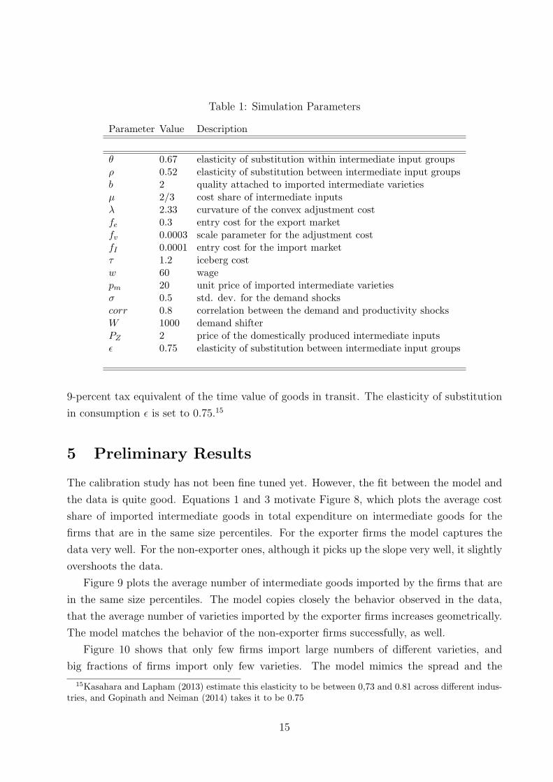
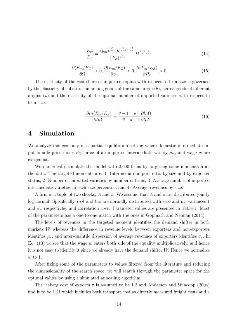
Table 1: Simulation Parameters

Parameter Value Description

θ 0.67 elasticity of substitution within intermediate input groupsρ 0.52 elasticity of substitution between intermediate input groupsb 2 quality attached to imported intermediate varietiesµ 2/3 cost share of intermediate inputsλ 2.33 curvature of the convex adjustment costfe 0.3 entry cost for the export marketfv 0.0003 scale parameter for the adjustment costfI 0.0001 entry cost for the import marketτ 1.2 iceberg costw 60 wagepm 20 unit price of imported intermediate varietiesσ 0.5 std. dev. for the demand shockscorr 0.8 correlation between the demand and productivity shocksW 1000 demand shifterPZ 2 price of the domestically produced intermediate inputsǫ 0.75 elasticity of substitution between intermediate input groups

9-percent tax equivalent of the time value of goods in transit. The elasticity of substitution

in consumption ǫ is set to 0.75.15

5 Preliminary Results

The calibration study has not been fine tuned yet. However, the fit between the model and

the data is quite good. Equations 1 and 3 motivate Figure 8, which plots the average cost

share of imported intermediate goods in total expenditure on intermediate goods for the

firms that are in the same size percentiles. For the exporter firms the model captures the

data very well. For the non-exporter ones, although it picks up the slope very well, it slightly

overshoots the data.

Figure 9 plots the average number of intermediate goods imported by the firms that are

in the same size percentiles. The model copies closely the behavior observed in the data,

that the average number of varieties imported by the exporter firms increases geometrically.

The model matches the behavior of the non-exporter firms successfully, as well.

Figure 10 shows that only few firms import large numbers of different varieties, and

big fractions of firms import only few varieties. The model mimics the spread and the

15Kasahara and Lapham (2013) estimate this elasticity to be between 0,73 and 0.81 across different indus-tries, and Gopinath and Neiman (2014) takes it to be 0.75

15

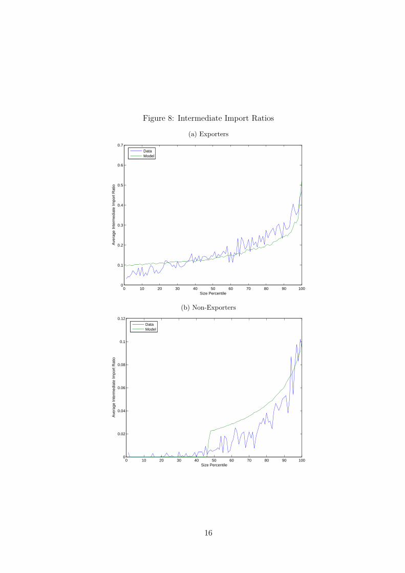
Figure 8: Intermediate Import Ratios

(a) Exporters

0 10 20 30 40 50 60 70 80 90 1000

0.1

0.2

0.3

0.4

0.5

0.6

0.7

Size Percentile

Ave

rage

Inte

rmed

iate

Impo

rt R

atio

DataModel

(b) Non-Exporters

0 10 20 30 40 50 60 70 80 90 1000

0.02

0.04

0.06

0.08

0.1

0.12

Size Percentile

Ave

rage

Inte

rmed

iate

Impo

rt R

atio

DataModel

16

Figure 9: Average Number of Imported Varieties by Firm Size

(a) Exporters

0 10 20 30 40 50 60 70 80 90 1000

20

40

60

80

100

120

140

160

Size Percentile

Ave

rage

Num

ber

of Im

port

ed V

arie

ties

DataModel

(b) Non-Exporters

0 10 20 30 40 50 60 70 80 90 1000

2

4

6

8

10

12

14

16

18

Size Percentile

Ave

rage

Num

ber

of Im

port

ed V

arie

ties

DataModel

17

slope observed in the data about the relationship between the number of different varieties

imported by a firm and the fraction of all firms that import such many varieties. However,

there is a level difference between the model and the data that should be worked out.

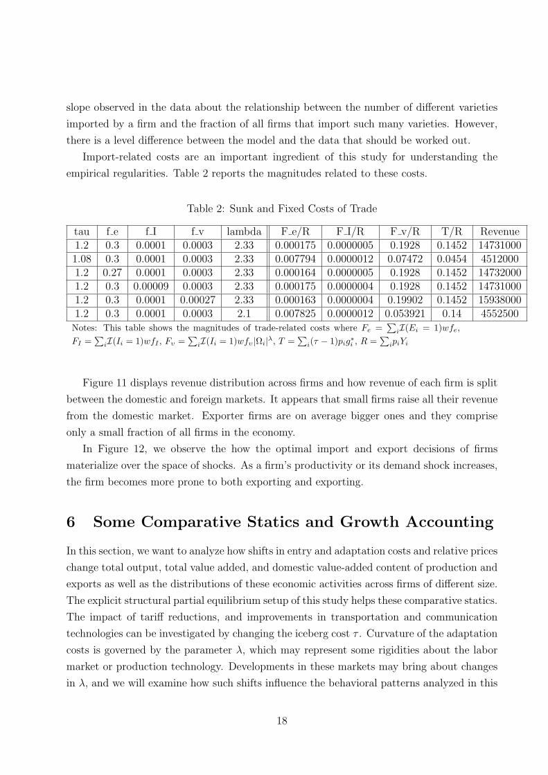
Import-related costs are an important ingredient of this study for understanding the

empirical regularities. Table 2 reports the magnitudes related to these costs.

Table 2: Sunk and Fixed Costs of Trade

tau f e f I f v lambda F e/R F I/R F v/R T/R Revenue1.2 0.3 0.0001 0.0003 2.33 0.000175 0.0000005 0.1928 0.1452 147310001.08 0.3 0.0001 0.0003 2.33 0.007794 0.0000012 0.07472 0.0454 45120001.2 0.27 0.0001 0.0003 2.33 0.000164 0.0000005 0.1928 0.1452 147320001.2 0.3 0.00009 0.0003 2.33 0.000175 0.0000004 0.1928 0.1452 147310001.2 0.3 0.0001 0.00027 2.33 0.000163 0.0000004 0.19902 0.1452 159380001.2 0.3 0.0001 0.0003 2.1 0.007825 0.0000012 0.053921 0.14 4552500Notes: This table shows the magnitudes of trade-related costs where Fe =

∑

iI(Ei = 1)wfe,

FI =∑

iI(Ii = 1)wfI , Fυ =

∑

iI(Ii = 1)wfυ|Ωi|

λ, T =∑

i(τ − 1)pig

∗

i, R =

∑

ipiYi

Figure 11 displays revenue distribution across firms and how revenue of each firm is split

between the domestic and foreign markets. It appears that small firms raise all their revenue

from the domestic market. Exporter firms are on average bigger ones and they comprise

only a small fraction of all firms in the economy.

In Figure 12, we observe the how the optimal import and export decisions of firms

materialize over the space of shocks. As a firm’s productivity or its demand shock increases,

the firm becomes more prone to both exporting and exporting.

6 Some Comparative Statics and Growth Accounting

In this section, we want to analyze how shifts in entry and adaptation costs and relative prices

change total output, total value added, and domestic value-added content of production and

exports as well as the distributions of these economic activities across firms of different size.

The explicit structural partial equilibrium setup of this study helps these comparative statics.

The impact of tariff reductions, and improvements in transportation and communication

technologies can be investigated by changing the iceberg cost τ . Curvature of the adaptation

costs is governed by the parameter λ, which may represent some rigidities about the labor

market or production technology. Developments in these markets may bring about changes

in λ, and we will examine how such shifts influence the behavioral patterns analyzed in this

18

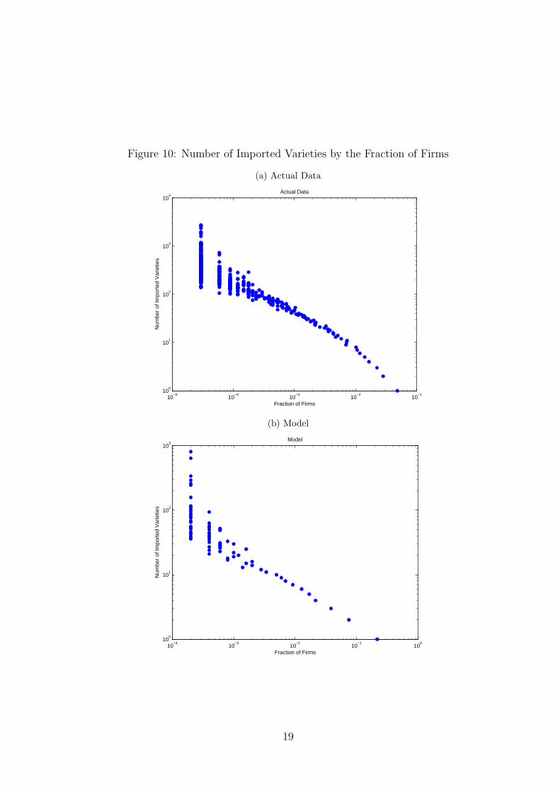
Figure 10: Number of Imported Varieties by the Fraction of Firms

(a) Actual Data

10−5

10−4

10−3

10−2

10−1

100

101

102

103

104

Actual Data

Fraction of Firms

Num

ber

of Im

port

ed V

arie

ties

(b) Model

10−4

10−3

10−2

10−1

100

100

101

102

103

Model

Fraction of Firms

Num

ber

of Im

port

ed V

arie

ties

19

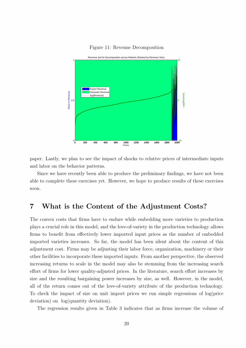
Figure 11: Revenue Decomposition

0 200 400 600 800 1000 1200 1400 1600 1800 20000

0.5

1

Sha

re in

Rev

enue

Revenue and Its Decomposition across Markets (Ranked by Revenue Size)

Firms

0 200 400 600 800 1000 1200 1400 1600 1800 2000−20

0

20

Log(

Rev

enue

)

Export RevenueDomestic Revenuelog(Revenue)

paper. Lastly, we plan to see the impact of shocks to relative prices of intermediate inputs

and labor on the behavior patterns.

Since we have recently been able to produce the preliminary findings, we have not been

able to complete these exercises yet. However, we hope to produce results of these exercises

soon.

7 What is the Content of the Adjustment Costs?

The convex costs that firms have to endure while embedding more varieties to production

plays a crucial role in this model, and the love-of-variety in the production technology allows

firms to benefit from effectively lower imported input prices as the number of embedded

imported varieties increases. So far, the model has been silent about the content of this

adjustment cost. Firms may be adjusting their labor force, organization, machinery or their

other facilities to incorporate these imported inputs. From another perspective, the observed

increasing returns to scale in the model may also be stemming from the increasing search

effort of firms for lower quality-adjusted prices. In the literature, search effort increases by

size and the resulting bargaining power increases by size, as well. However, in the model,

all of the return comes out of the love-of-variety attribute of the production technology.

To check the impact of size on unit import prices we run simple regressions of log(price

deviation) on log(quantity deviation).

The regression results given in Table 3 indicates that as firms increase the volume of

20

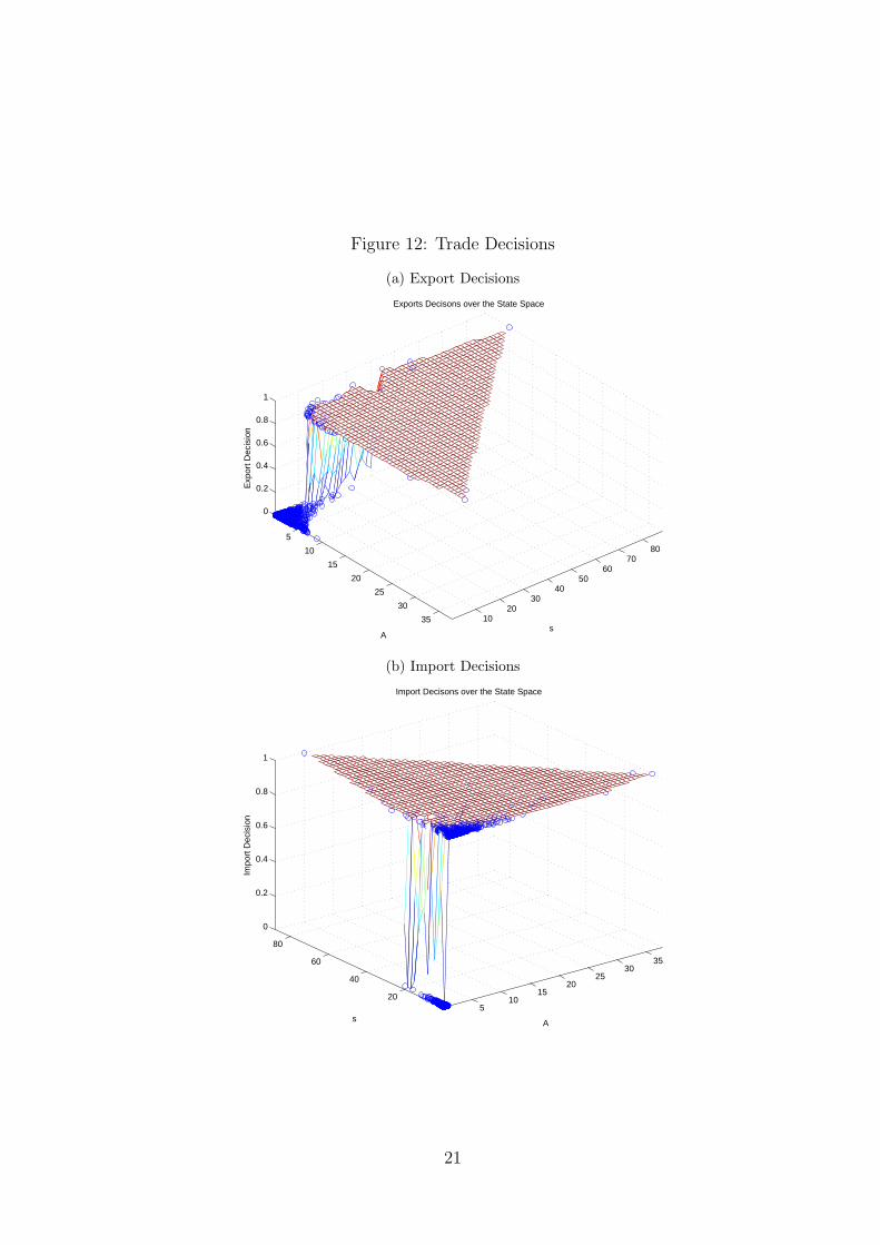
Figure 12: Trade Decisions

(a) Export Decisions

5

10

15

20

25

30

35 1020

3040

5060

7080

0

0.2

0.4

0.6

0.8

1

s

Exports Decisons over the State Space

A

Exp

ort D

ecis

ion

(b) Import Decisions

510

1520

2530

35

20

40

60

80

0

0.2

0.4

0.6

0.8

1

A

Import Decisons over the State Space

s

Impo

rt D

ecis

ion

21

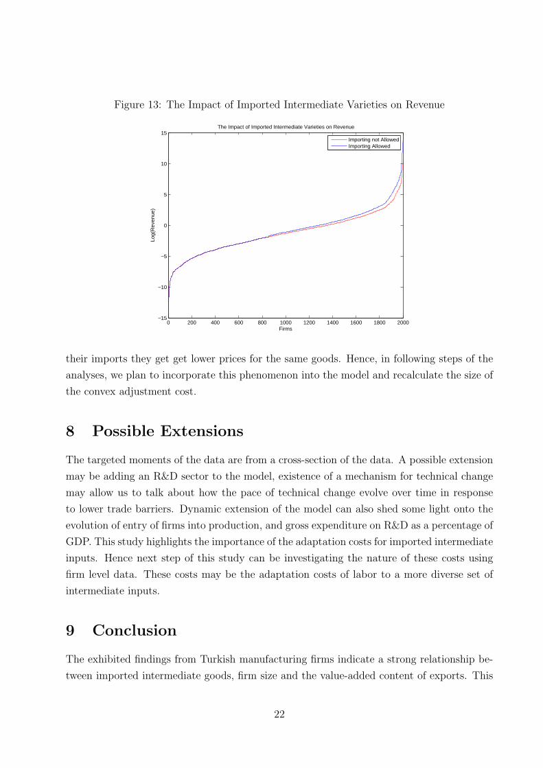
Figure 13: The Impact of Imported Intermediate Varieties on Revenue

0 200 400 600 800 1000 1200 1400 1600 1800 2000−15

−10

−5

0

5

10

15

Firms

Log(

Rev

enue

)

The Impact of Imported Intermediate Varieties on Revenue

Importing not AllowedImporting Allowed

their imports they get get lower prices for the same goods. Hence, in following steps of the

analyses, we plan to incorporate this phenomenon into the model and recalculate the size of

the convex adjustment cost.

8 Possible Extensions

The targeted moments of the data are from a cross-section of the data. A possible extension

may be adding an R&D sector to the model, existence of a mechanism for technical change

may allow us to talk about how the pace of technical change evolve over time in response

to lower trade barriers. Dynamic extension of the model can also shed some light onto the

evolution of entry of firms into production, and gross expenditure on R&D as a percentage of

GDP. This study highlights the importance of the adaptation costs for imported intermediate

inputs. Hence next step of this study can be investigating the nature of these costs using

firm level data. These costs may be the adaptation costs of labor to a more diverse set of

intermediate inputs.

9 Conclusion

The exhibited findings from Turkish manufacturing firms indicate a strong relationship be-

tween imported intermediate goods, firm size and the value-added content of exports. This

22

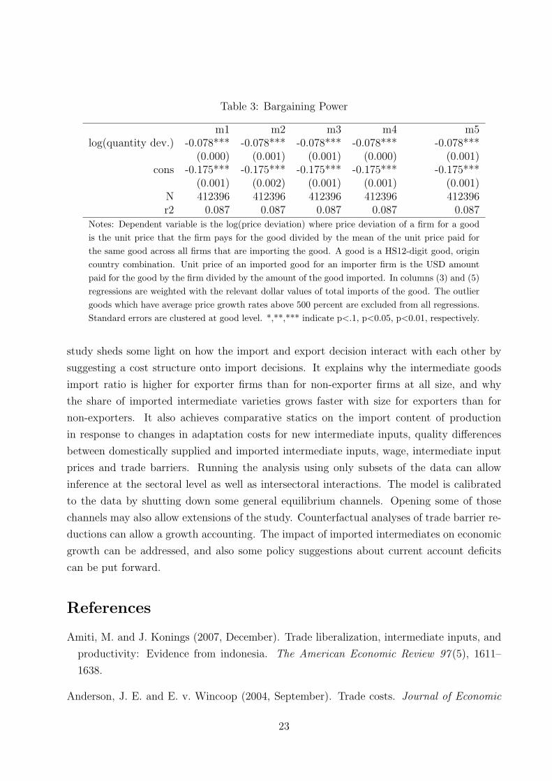
Table 3: Bargaining Power

m1 m2 m3 m4 m5log(quantity dev.) -0.078*** -0.078*** -0.078*** -0.078*** -0.078***

(0.000) (0.001) (0.001) (0.000) (0.001)cons -0.175*** -0.175*** -0.175*** -0.175*** -0.175***

(0.001) (0.002) (0.001) (0.001) (0.001)N 412396 412396 412396 412396 412396r2 0.087 0.087 0.087 0.087 0.087

Notes: Dependent variable is the log(price deviation) where price deviation of a firm for a good

is the unit price that the firm pays for the good divided by the mean of the unit price paid for

the same good across all firms that are importing the good. A good is a HS12-digit good, origin

country combination. Unit price of an imported good for an importer firm is the USD amount

paid for the good by the firm divided by the amount of the good imported. In columns (3) and (5)

regressions are weighted with the relevant dollar values of total imports of the good. The outlier

goods which have average price growth rates above 500 percent are excluded from all regressions.

Standard errors are clustered at good level. *,**,*** indicate p<.1, p<0.05, p<0.01, respectively.

study sheds some light on how the import and export decision interact with each other by

suggesting a cost structure onto import decisions. It explains why the intermediate goods

import ratio is higher for exporter firms than for non-exporter firms at all size, and why

the share of imported intermediate varieties grows faster with size for exporters than for

non-exporters. It also achieves comparative statics on the import content of production

in response to changes in adaptation costs for new intermediate inputs, quality differences

between domestically supplied and imported intermediate inputs, wage, intermediate input

prices and trade barriers. Running the analysis using only subsets of the data can allow

inference at the sectoral level as well as intersectoral interactions. The model is calibrated

to the data by shutting down some general equilibrium channels. Opening some of those

channels may also allow extensions of the study. Counterfactual analyses of trade barrier re-

ductions can allow a growth accounting. The impact of imported intermediates on economic

growth can be addressed, and also some policy suggestions about current account deficits

can be put forward.

References

Amiti, M. and J. Konings (2007, December). Trade liberalization, intermediate inputs, and

productivity: Evidence from indonesia. The American Economic Review 97 (5), 1611–

1638.

Anderson, J. E. and E. v. Wincoop (2004, September). Trade costs. Journal of Economic

23

Literature 42 (3), 691–751.

Bergin, P. R., R. C. Feenstra, and G. H. Hanson (2009). Offshoring and volatility: Evidence

from mexico’s maquiladora industry. American Economic Review 99 (4), 1664–1671.

Feenstra, R. C. and G. H. Hanson (1997, May). Foreign direct investment and relative wages:

Evidence from mexico’s maquiladoras. Journal of International Economics 42 (3-4), 371–

393.

Goldberg, P. K., A. K. Khandelwal, N. Pavcnik, and P. Topalova (2010, November). Imported

intermediate inputs and domestic product growth: Evidence from india. The Quarterly

Journal of Economics 125 (4), 1727 –1767.

Gopinath, G. and B. Neiman (2014). Trade adjustment and productivity in large crises.

American Economic Review .

Grossman, G. M. and E. Rossi-Hansberg (2008, December). Trading tasks: A simple theory

of offshoring. The American Economic Review 98 (5), 1978–1997.

Halpern, L., M. Koren, and A. Szeidl (2011). Imported inputs and productivity. mimeo.

Hummels, D., J. Ishii, and K.-M. Yi (2001, June). The nature and growth of vertical

specialization in world trade. Journal of International Economics 54 (1), 75–96.

Johnson, R. C. and G. Noguera (2012). Accounting for intermediates: Production sharing

and trade in value added. Journal of International Economics .

Kasahara, H. and B. Lapham (2013, March). Productivity and the decision to import and

export: Theory and evidence. Journal of International Economics 89 (2), 297–316.

Kasahara, H. and J. Rodrigue (2008, August). Does the use of imported intermediates

increase productivity? plant-level evidence. Journal of Development Economics 87 (1),

106–118.

Melitz, M. J. (2003, November). The impact of trade on intra-industry reallocations and

aggregate industry productivity. Econometrica 71 (6), 1695–1725.

Saygl, S., C. Cihan, C. Yalcin, and T. Hamsici (2010). Turkiye malat sanayiinin thalat yaps.

TCMB WP No:1002 .

APPENDIX

24

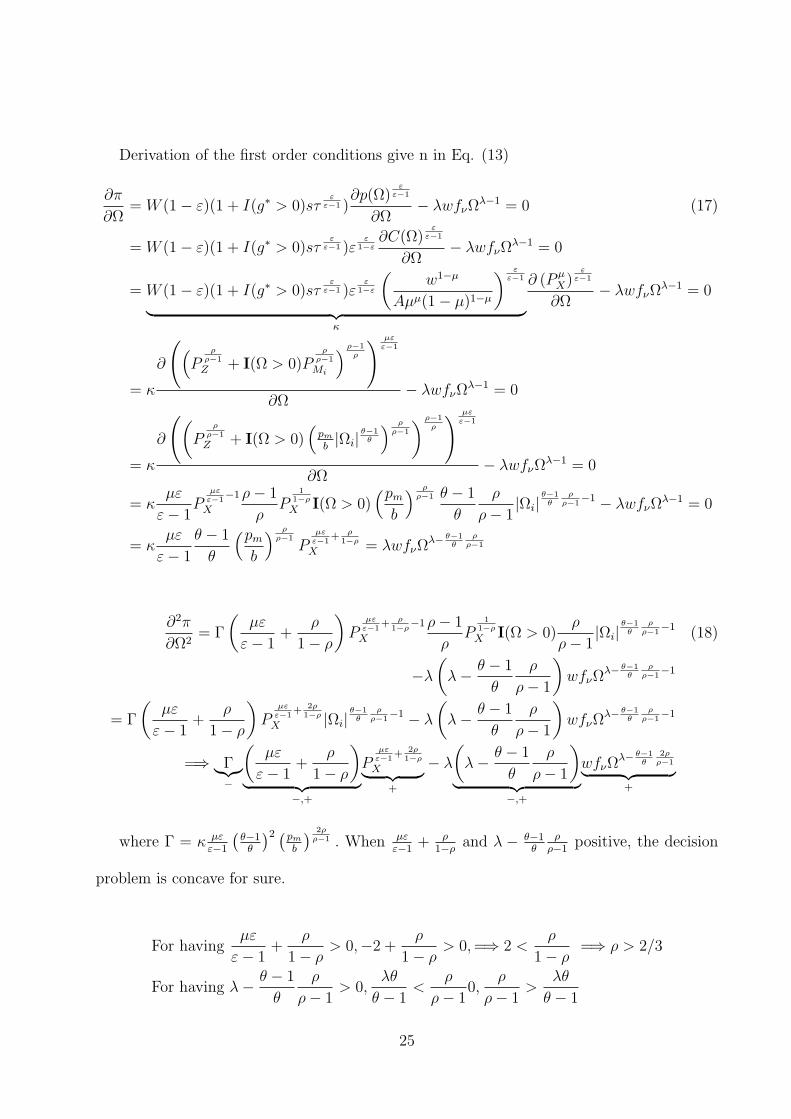
Derivation of the first order conditions give n in Eq. (13)

∂π

∂Ω= W (1− ε)(1 + I(g∗ > 0)sτ

εε−1 )

∂p(Ω)ε

ε−1

∂Ω− λwfνΩ

λ−1 = 0 (17)

= W (1− ε)(1 + I(g∗ > 0)sτε

ε−1 )εε

1−ε∂C(Ω)

εε−1

∂Ω− λwfνΩ

λ−1 = 0

= W (1− ε)(1 + I(g∗ > 0)sτε

ε−1 )εε

1−ε

(w1−µ

Aµµ(1− µ)1−µ

) εε−1

︸ ︷︷ ︸

κ

∂ (P µX)

εε−1

∂Ω− λwfνΩ

λ−1 = 0

= κ

∂

((

Pρ

ρ−1

Z + I(Ω > 0)Pρ

ρ−1

Mi

) ρ−1

ρ

) µεε−1

∂Ω− λwfνΩ

λ−1 = 0

= κ

∂

((

Pρ

ρ−1

Z + I(Ω > 0)(

pmb|Ωi|

θ−1

θ

) ρρ−1

) ρ−1

ρ

) µεε−1

∂Ω− λwfνΩ

λ−1 = 0

= κµε

ε− 1P

µεε−1

−1

X

ρ− 1

ρP

1

1−ρ

X I(Ω > 0)(pm

b

) ρρ−1 θ − 1

θ

ρ

ρ− 1|Ωi|

θ−1

θρ

ρ−1−1 − λwfνΩ

λ−1 = 0

= κµε

ε− 1

θ − 1

θ

(pmb

) ρρ−1

Pµεε−1

+ ρ1−ρ

X = λwfνΩλ− θ−1

θρ

ρ−1

∂2π

∂Ω2= Γ

(µε

ε− 1+

ρ

1− ρ

)

Pµεε−1

+ ρ1−ρ

−1

X

ρ− 1

ρP

1

1−ρ

X I(Ω > 0)ρ

ρ− 1|Ωi|

θ−1

θρ

ρ−1−1 (18)

−λ

(

λ−θ − 1

θ

ρ

ρ− 1

)

wfνΩλ− θ−1

θρ

ρ−1−1

= Γ

(µε

ε− 1+

ρ

1− ρ

)

Pµεε−1

+ 2ρ1−ρ

X |Ωi|θ−1

θρ

ρ−1−1 − λ

(

λ−θ − 1

θ

ρ

ρ− 1

)

wfνΩλ− θ−1

θρ

ρ−1−1

=⇒ Γ︸︷︷︸

−

(µε

ε− 1+

ρ

1− ρ

)

︸ ︷︷ ︸

−,+

Pµεε−1

+ 2ρ1−ρ

X︸ ︷︷ ︸

+

− λ

(

λ−θ − 1

θ

ρ

ρ− 1

)

︸ ︷︷ ︸

−,+

wfνΩλ− θ−1

θ2ρρ−1

︸ ︷︷ ︸

+

where Γ = κ µε

ε−1

(θ−1θ

)2 (pmb

) 2ρρ−1 . When µε

ε−1+ ρ

1−ρand λ − θ−1

θ

ρ

ρ−1positive, the decision

problem is concave for sure.

For havingµε

ε− 1+

ρ

1− ρ> 0,−2 +

ρ

1− ρ> 0,=⇒ 2 <

ρ

1− ρ=⇒ ρ > 2/3

For having λ−θ − 1

θ

ρ

ρ− 1> 0,

λθ

θ − 1<

ρ

ρ− 10,

ρ

ρ− 1>

λθ

θ − 1

25

Ifλθ

1− θ>

ρ

1− ρ> 2

Ifλθ

1− θ>

ρ

1− ρ> 2

then Γ︸︷︷︸

−

(µε

ε− 1+

ρ

1− ρ

)

︸ ︷︷ ︸

+

Pµεε−1

+ 2ρ1−ρ

X︸ ︷︷ ︸

+

︸ ︷︷ ︸

−

− λ

(

λ−θ − 1

θ

ρ

ρ− 1

)

︸ ︷︷ ︸

+

wfνΩλ− θ−1

θ2ρρ−1

︸ ︷︷ ︸

+

︸ ︷︷ ︸

+

26