Durability of Output and Expected Stock Returns∗

Joao F. Gomes†, Leonid Kogan‡, and Motohiro Yogo§

Abstract

The demand for durable goods is more cyclical than that for nondurable goods

and services. Consequently, the cash flow and stock returns of durable-good produc-

ers are exposed to higher systematic risk. Using the NIPA input-output tables, we

construct portfolios of durable-good, nondurable-good, and service producers. In the

cross-section, a strategy that is long on durables and short on services earns a sizable

risk premium. In the time series, a strategy that is long on durables and short on

the market portfolio earns a countercyclical risk premium. We develop an equilibrium

asset-pricing model that explains these empirical findings.

JEL classification: D57; E21; G12

Keywords: Cash flow; Durable goods; Factor-mimicking portfolios; Input-output ac-

counts; Stock returns

First draft: December 16, 2005

This draft: January 12, 2007

∗For comments and discussions, we thank James Choi, Lars Hansen, Robert Stambaugh, Selale Tuzel, andseminar participants at the Federal Reserve Board, Goldman Sachs, UBC, University of Chicago, Universityof Tokyo, University of Utah, University of Washington, Wharton, North American Winter Meeting of theEconometric Society 2006, and NYU Stern Five-Star Conference 2006.

†The Wharton School, University of Pennsylvania, 3620 Locust Walk, Philadelphia, PA 19104 (e-mail:gomesj@wharton.upenn.edu).

‡Sloan School of Management, MIT, 50 Memorial Drive, E52-455, Cambridge, MA 02142 (e-mail: lko-gan@mit.edu).

§The Wharton School, University of Pennsylvania, 3620 Locust Walk, Philadelphia, PA 19104 (e-mail:yogo@wharton.upenn.edu).

1 Introduction

The cross-section of stock returns has been a subject of considerable research in financial

economics. A key finding in this literature is that variation in accounting and financial

variables across stocks generates puzzlingly large variation in average returns.1 In contrast,

variation in measured systematic risk across stocks generates surprisingly little variation in

average returns. For instance, classic studies of the capital asset pricing model (CAPM)

have found no variation in average returns across portfolios of stocks sorted by the market

beta (Black, Jensen, and Scholes 1972, Fama and MacBeth 1973, Fama and French 1992).

In this paper, we show that an important source of systematic risk is priced in the cross-

section of stock returns. Our approach builds on the core intuition of the consumption-based

CAPM, which dictates that assets with higher exposure to consumption risk command higher

risk premia. Because some components of aggregate consumption are more cyclical than

others, firms producing the more cyclical components must command higher risk premia.

Specifically, we argue theoretically and verify empirically that firms that produce durable

goods are exposed to higher systematic risk than those that produce nondurable goods

and services. An appealing aspect of our approach is that we classify firms based on an

easily observable and economically meaningful source of systematic risk, rather than ad hoc

characteristics that have tenuous relationship with risk. While durability is probably not

the only aspect of a firm’s output that determines its exposure to consumption risk, our

empirical success provides hope for identifying other proxies for systematic risk that are tied

to variation in expected returns.

To identify the durability of each firm’s output, we first develop a novel industry classifi-

cation using the Benchmark Input-Output Accounts. This classification essentially identifies

each Standard Industrial Classification (SIC) industry by its primary contribution to fi-

1A partial list of accounting and financial variables that are known to be related to average stock returnsare market equity (Banz 1981), earnings yield (Basu 1983), book-to-market equity (Rosenberg, Reid, andLanstein 1985, Fama and French 1992), leverage (Bhandari 1988), and past returns (Jegadeesh and Titman1993).

2

nal demand. We then sort firms into portfolios representing the three broad categories of

personal consumption expenditures (PCE): durable goods, nondurable goods, and services.

Because these portfolios have cash flows that are economically tied to aggregate consumption,

they can be interpreted as consumption-risk mimicking portfolios in the sense of Breeden,

Gibbons, and Litzenberger (1989).

We use these PCE portfolios to document four main facts about the durable portfolio,

relative to the service or the nondurable portfolio.

1. The durable portfolio has cash flows that are more volatile and more correlated with

aggregate consumption.

2. The durable portfolio has returns that are higher on average and more volatile. Over

the period 1927–2004, a strategy that is long on durables and short on services earned

an average annual rate of return of almost 4.5%.

3. The durable portfolio has cash flows that are conditionally more volatile when the ratio

of aggregate durable expenditure to its stock is low.

4. The durable portfolio has returns that are more predictable. A strategy that is long

on durables and short on the market portfolio has countercyclical expected returns

that are strongly predicted by the durable expenditure-stock ratio. Moreover, the

conditional covariance of this strategy’s returns with durable consumption growth is

countercyclical, suggesting that this variation in expected returns is compensation for

consumption risk.

To better understand these empirical findings, we develop an equilibrium asset-pricing

model that extends the two-good endowment model of Dunn and Singleton (1986), Eichen-

baum and Hansen (1990), and Piazzesi, Schneider, and Tuzel (2006). Specifically, we set up

a two-sector economy in which optimal resource allocation endogenously generates the out-

put of a durable-good and a nondurable-good producer. The firm’s output then determines

3

the joint process for its cash flow and asset return. Although our model is a simplified de-

scription of reality, designed to make transparent the basic economic mechanism, it delivers

most of our key empirical findings in the cross-section of returns.

The key results of the model are driven by two intuitive mechanisms. First, a proportional

change in the service flow of durables (i.e., the stock) requires a much larger proportional

change in its expenditure (i.e., the investment). As a result, the demand for durable goods is

more cyclical and volatile than that for nondurable goods. Because the cash flow of durable-

good producers is exposed to higher systematic risk, their unconditional expected returns are

higher than those of nondurable-good producers. Second, the magnitude of the proportional

change in expenditure must be relatively large when the existing stock of durables is high

relative to current demand. Because the cash flow of durable-good producers is exposed to

higher systematic risk when the stock of durables is high relative to its expenditure, their

conditional expected returns are more time varying than those of nondurable-good producers.

Although the model successfully explains our key empirical findings in the cross-section

of returns, it is clearly too simple to match all of the standard asset-pricing facts. In par-

ticular, the model fails to match the high volatility of stock returns and the magnitude of

time variation in the equity premium. Although the ingredients necessary to resolve the

classic asset-pricing puzzles within the consumption-based framework are now well known,

we abstract from these issues to highlight the basic intuition for our findings (see Campbell

and Cochrane (1999) and Bansal and Yaron (2004)).

Our work is part of a recent effort to link expected returns to fundamental aspects of

firm heterogeneity. One branch of the literature shows that the size and book-to-market

effects arise naturally from optimal production and investment decisions.2 A limitation of

these earlier studies is that the underlying determinants of stock returns are often difficult

to measure, and perhaps more significantly, they reflect fundamental differences between

2See, for example, Berk, Green, and Naik (1999), Kogan (2001, 2004), Gomes, Kogan, and Zhang (2003),Carlson, Fisher, and Giammarino (2004), Gala (2006), and Zhang (2006).

4

firms that are not true primitives of the economic environment.3 Partly in response, Gourio

(2005) and Tuzel (2005) focus on more readily identifiable sources of firm heterogeneity, such

as differences in their production technology or the composition of their physical assets. This

paper is in the same spirit, but we focus on heterogeneity in the characteristics of the output,

rather than the inputs or technology.

The remainder of the paper proceeds as follows. In Section 2, we motivate the basic

idea by documenting empirical properties of portfolios sorted by the durability of output.

In Section 3, we set up a simple two-sector economy that incorporates the notion of firm

heterogeneity based on the durability of output. In Section 4, we calibrate the model to

match aggregate quantities and examine its asset-pricing implications. In Section 5, we

document cross-sectional and time-series evidence for an empirical relationship between risk

and return. Section 6 concludes. A separate appendix (Gomes, Kogan, and Yogo 2006)

contains the industry classification as well as a documentation of its construction.

2 Portfolios Sorted by the Durability of Output

2.1 Industry Classification

The National Income and Product Accounts (NIPA) divides PCE into the following three

categories, ordered in decreasing degree of durability.

• Durable goods are “commodities that can be stored or inventoried and have an average

service life of at least three years.” This category consists of furniture and household

equipment; motor vehicles and parts; and other durable goods.

• Nondurable goods are “commodities that can be stored or inventoried and have an

average service life of at most three years.” This category consists of clothing and

shoes; food; fuel oil and coal; gasoline and oil; and other nondurable goods.

3Key ingredients in these models include heterogeneity in fixed costs of operation, the degree of irre-versibility in capital, and the volatility of cash flow.

5

• Services are “commodities that cannot be stored and that are consumed at the place

and time of purchase.” This category consists of household operation; housing4; med-

ical care; net foreign travel; personal business; personal care; private education and

research; recreation; religious and welfare activities; and transportation.

Our empirical analysis requires a link from industries, identified at the four-digit SIC code,

to the various components of PCE. Because such a link is not readily available, we create our

own using NIPA’s Benchmark Input-Output Accounts (Bureau of Economic Analysis 1994).

The input-output accounts identify how much output each industry contributes to the four

broad categories of final demand: PCE, gross private investment, government expenditures,

and net exports of goods and services. Within PCE, the input-output accounts also identify

how much output each industry contributes to the three categories of durability. Based

on this data, we assign each industry to the category of final demand to which it has the

highest value added: PCE on durable goods, PCE on nondurable goods, PCE on services,

investment, government expenditures, and net exports. Gomes, Kogan, and Yogo (2006)

contains further details on the construction of the industry classification.

2.2 Construction of the Portfolios

The universe of stocks is ordinary common equity traded in NYSE, AMEX, or Nasdaq,

which are recorded in the Center for Research in Securities Prices (CRSP) Monthly Stock

Database. In June of each year t, we sort the universe of stocks into five industry portfolios

based on their SIC code: services, nondurable goods, durable goods, investment, and other

industries. Other industries include the wholesale, retail, and financial sectors as well as

industries whose primary output is to government expenditures or net exports. The stock

must have a non-missing SIC code in order to be included in a portfolio. We first search for

4According to the input-output accounts, SIC 7000 (hotels and other lodging places) is the only industrythat has direct output to housing services. Expenditure on owner-occupied housing is accounted as partof residential fixed investment, rather than PCE. In the publicly available files, the input-output accountsdo not have a breakdown of fixed investment into residential and nonresidential. Therefore, owner-occupiedhousing will remain outside the scope of our analysis of durable goods.

6

a match at the four-, then at the three-, and finally at the two-digit SIC. Once the portfolios

are formed, we track their value-weighted returns from July of year t through June of year

t + 1. We compute annual portfolio returns by compounding monthly returns.

We compute dividends for each stock based on the difference of holding period returns

with and without dividends. Since 1971, we augment dividends with equity repurchase

(Item 115) from Compustat’s statement of cash flows (Boudoukh, Michaely, Richardson,

and Roberts 2007). We assume that the repurchases occur at the end of each fiscal year.

Monthly dividends for each portfolio are simply the sum of dividends across all stocks in the

portfolio. We compute annual dividends in December of each year by accumulating monthly

dividends, assuming that intermediate (January through November) dividends are reinvested

in the portfolio until the end of the calendar year. We compute dividend growth and the

dividend yield for each portfolio based on a “buy and hold” investment strategy starting in

1927.

Since 1951, we compute other properties for each portfolio using the subset of firms for

which the relevant data are available from Compustat. Book-to-market equity is book equity

at the end of fiscal year t divided by the market equity in December of year t. Liabilities-

to-market equity is liabilities (Item 181) at the end of fiscal year t divided by the market

equity in December of year t. We construct book equity data as a merge of Compustat and

historical data from Moody’s Manuals, available through Kenneth French’s webpage. We

follow the procedure described in Davis, Fama, and French (2000) for the computation of

book equity. Operating income is sales (Item 12) minus the cost of goods sold (Item 41).

We compute the annual growth rate of sales and operating income in each year t based on

the subset of firms that are in the portfolio in years t − 1 and t.

By construction, the three PCE portfolios have cash flows that are directly tied to con-

sumption expenditures. We therefore interpret them as consumption-risk mimicking port-

folios. The notion of synthesizing assets that mimic macroeconomic risk is hardly new (see

Shiller (1993)). However, our methodology differs from the conventional procedure that

7

starts with a universe of assets, and then estimates portfolio weights that create maximal

correlation with the economic variable of interest (e.g., Breeden, Gibbons, and Litzenberger

(1989) and Lamont (2001)). Our procedure does not require estimation, and more impor-

tantly, the cash flows are economically (rather than just statistically) linked to consumption

risk.

2.3 Portfolio Properties

Table 1 reports some basic properties of the five industry portfolios. We focus our attention

on the first three portfolios, which represent PCE. To get a sense of the size of the portfolios,

we report the average number of firms and the average share of total market equity that each

portfolio represents. In the full sample period, services represent 15%, nondurables represent

35%, and durables represent 16% of total market equity. On average, the service portfolio

has the highest, and the nondurable portfolio has the lowest dividend yield.

For the sample period 1951–2004, we also report log book-to-market equity and log

liabilities-to-market equity. On average, the service portfolio has the highest, and the non-

durable portfolio has the lowest book-to-market equity. Similarly, the service portfolio has

the highest, and the nondurable portfolio has the lowest liabilities-to-market equity. These

patterns suggest that durability is not a property that is directly related to the book-to-

market and leverage effects in expected stock returns.

2.4 Link to Aggregate Consumption

If our procedure successfully identifies durable-good producers, the total sales of firms in

the durable portfolio should be empirically related to the aggregate expenditure on durable

goods. In Figure 1, we plot the annual growth rate of sales for the service, the nondurable,

and the durable portfolio. The dashed line in all three panels, shown for the purposes of

comparison, is the growth rate of real durable expenditure from NIPA. As shown in Panel C,

the correlation between sales of the durable portfolio and durable expenditure is almost

8

perfect, except in the last ten years.5 This evidence suggests that our industry classification

based on the input-output tables successfully identifies durable-good producers.

Table 2 reports the same evidence in a more systematic way. Panel A reports descriptive

statistics for the annual growth rate of sales for the PCE portfolios. In addition, the table

reports the correlation between sales growth and the growth rate of real service consump-

tion, nondurable consumption, and durable expenditure. (Appendix A contains a detailed

description of the consumption data.) The durable portfolio has sales that are more volatile

than those of the service or the nondurable portfolio with a standard deviation of 8%. The

sales of the durable portfolio have correlation of 0.81 with durable expenditure, confirming

the visual impression in Figure 1. The sales of both the service and the nondurable portfolio

have relatively low correlation with nondurable and service consumption. An explanation for

this low correlation is that a large part of nondurable and service consumption is produced

by private firms, nonprofit firms, and households that are not part of the CRSP database.

There is a potential accounting problem in aggregating sales across firms. Conceptually,

aggregate consumption in NIPA is the sum of value added across firms, which is sales minus

the cost of intermediate inputs. Therefore, the sum of sales across firms can lead to double

accounting of the cost of intermediate inputs. We therefore compute the operating income

for each firm, defined as sales minus the cost of goods sold. Unfortunately, the cost of goods

sold in Compustat includes wages and salaries in addition to the cost of intermediate inputs.

However, this adjustment would eliminate double accounting and potentially give us a better

correspondence between the output of Compustat firms and aggregate consumption.

Panel B reports descriptive statistics for the annual growth rate of operating income for

the PCE portfolios. The standard deviation of operating-income growth for the durable

portfolio is 13%, compared to 6% for the service and the nondurable portfolio. These dif-

ferences mirror the large differences in the volatility of real aggregate quantities. In the

full sample, the standard deviation of nondurable and service consumption growth is 2%,

5We suspect that foreign firms, producing motor vehicles and appliances in the U.S., have become animportant part of durable expenditure in the recent period.

9

compared to 13% for durable expenditure growth (see Table 7). In comparison to sales, the

operating income of the service and the nondurable firms have much higher correlation with

nondurable and service consumption. The correlation between the operating income of the

service portfolio and service consumption is 0.25, and the correlation between the operating

income of the nondurable portfolio and nondurable consumption is 0.31. The correlation

between the operating income of the durable portfolio and durable expenditure is 0.79.

The fundamental economic mechanism in this paper is that durable-good producers have

demand that is more cyclical than that of nondurable-good producers. Table 2 provides

strong empirical support for this mechanism, consistent with previous findings by Petersen

and Strongin (1996). In the Census of Manufacturing for the period 1958–1986, they find

that durable manufacturers are three times more cyclical than nondurable manufacturers, as

measured by the elasticity of output (i.e., value added) to gross national product. Moreover,

they find that this difference in cyclicality is driven by demand, rather than factors that

affect supply (e.g., factor intensities, industry concentration, and unionization).

2.5 Stock Returns

Table 3 reports descriptive statistics for excess returns (over the three-month T-bill) on the

five industry portfolios. In the period 1927–2004, both the average and the standard devia-

tion of returns rise in the durability of output. Excess returns on the service portfolio has

mean of 5.99% and a standard deviation of 18.70%. Excess returns on the durable portfolio

has mean of 10.40% and a standard deviation of 29.27%. In ten-year sub-samples, durables

generally have higher average returns than both services and nondurables. Interestingly,

the largest spread in average returns occurred in the period 1927–1934, during the Great

Depression. The spread between durables and nondurables is almost 8%, and the spread

between nondurables and services is over 6%.

10

2.6 Predictability of Returns

Panel A of Table 4 examines evidence for the predictability of excess returns on the PCE

portfolios. Our main predictor variable is durable expenditure as a fraction of its stock,

which captures the strength of demand for durable goods over the business cycle. As shown

in Panel A of Figure 2, the durable expenditure-stock ratio is strongly procyclical, peaking

during expansions as identified by the National Bureau of Economic Research (NBER).

We report results for the full sample 1930–2004 and the postwar sample 1951–2004. The

postwar sample is commonly used in empirical work due to apparent non-stationarity in

durable expenditure during and immediately after the war (e.g., Ogaki and Reinhart (1998)

and Yogo (2006)). We focus our discussion on the postwar sample because the results are

qualitatively similar for the full sample.

In an univariate regression, the durable expenditure-stock ratio predicts excess returns on

the service portfolio with a coefficient of −0.75, the nondurable portfolio with a coefficient

of −0.14, and the durable portfolio with a coefficient of −1.11. The negative coefficient

across the portfolios implies that the durable expenditure-stock ratio predicts the common

countercyclical component of expected returns. This finding is similar to a previous finding

that the ratio of investment to the capital stock predicts aggregate stock returns (Cochrane

1991). Of more interest than the common sign is the relative magnitude of the coefficient

across the portfolios. The coefficient is the most negative for the durable portfolio, implying

that it has the largest amount of countercyclical variation in expected returns.

In order to assess the strength of the evidence for return predictability, Table 4 also exam-

ines a bivariate regression that includes each portfolio’s own dividend yield. The coefficient

for the durable expenditure-stock ratio is hardly changed from the univariate regression. The

dividend yield predicts excess returns with a positive coefficient as expected, but adds little

predictive power over the durable expenditure-stock ratio in terms of the R2.

In Panel B, we examine whether there is cyclical variation in the volatility of returns.

Rather than a structural estimation of risk and return, which we implement in Section 5, we

11

report here a simple regression of absolute excess returns onto the lagged predictor variables.

In an univariate regression, the durable expenditure-stock ratio predicts absolute excess

returns on the service portfolio with a coefficient of 0.12, the nondurable portfolio with

a coefficient of 0.16, and the durable portfolio with a coefficient of −0.18. While these

coefficients are not statistically significant in the postwar sample, the empirical pattern

suggests that the volatility of returns on the durable portfolio is more countercyclical than

that of the service or the nondurable portfolio.

2.7 Predictability of Cash-Flow Volatility

Differences in the conditional risk of the PCE portfolios are difficult to isolate based on

returns data alone. This difficulty could arise from the fact that returns are driven by both

news about aggregate discount rates and news about industry-specific cash flows. In Table 5,

we therefore examine evidence for the predictability of cash-flow volatility. The basic idea is

that the conditional risk on the PCE portfolios should be predictable because their returns

are predictable. We use the same predictor variables as those used for predicting returns in

Table 4.

As reported in Panel A, the durable expenditure-stock ratio predicts absolute sales growth

for the service portfolio with a coefficient of 0.14, the nondurable portfolio with a coefficient

of 0.25, and the durable portfolio with a coefficient of −0.20. This empirical pattern suggests

that the volatility of cash-flow growth for the durable portfolio is more countercyclical than

that for the service or the nondurable portfolio. The evidence is robust to including the

dividend yield as an additional regressor, and to using operating income instead of sales as

the measure of cash flow.

In Panel C, we examine evidence for the predictability of the volatility of five-year div-

idend growth. We motivate five-year dividend growth as a way to empirically implement

the cash-flow news component of a standard return decomposition (Campbell 1991). The

durable expenditure-stock ratio predicts absolute dividend growth for the service portfo-

12

lio with a coefficient of 0.15, the nondurable portfolio with a coefficient of −1.17, and the

durable portfolio with a coefficient of −1.46. This evidence suggests that the cash flow of

the durable portfolio is exposed to higher systematic risk than that of the service or the

nondurable portfolio during recessions, when durable expenditure is low relative to its stock.

3 Asset-Pricing Model

The last section established two key facts about the cash flow and returns of durable-good

producers in comparison to those of nondurable-good producers. First, the cash flow of

durable-good producers is more volatile and more correlated with aggregate consumption.

This unconditional cash-flow risk appears to explain the fact that durable-good producers

have higher average returns than nondurable-good producers. Second, the cash flow of

durable-good producers is more volatile when the durable expenditure-stock ratio is low.

This conditional cash-flow risk appears to explain the fact that durable-good producers have

expected returns that are more time varying than those of nondurable-good producers.

In this section, we construct an equilibrium asset-pricing model as an organizing frame-

work for our empirical findings. We begin with a representative-household model as in Yogo

(2006), then endogenize the production of nondurable and durable consumption goods. Our

analysis highlights the role of durability as an economic mechanism that generates differ-

ences in firm output and cash-flow risk, abstracting from other sources of asymmetry. The

model delivers most of our key empirical findings in a simple and parsimonious setting. It

also provides the necessary theoretical structure to guide our formal econometric tests in

Section 5.

3.1 Representative Household

There is an infinitely lived representative household in an economy with a complete set

of financial markets. In each period t, the household purchases Ct units of a nondurable

13

consumption good and Et units of a durable consumption good. The nondurable good is

taken to be the numeraire, so that Pt denotes the price of the durable good in units of

the nondurable good. The nondurable good is entirely consumed in the period of purchase,

whereas the durable good provides service flows for more than one period. The household’s

stock of the durable good Dt is related to its expenditure by the law of motion

Dt = (1 − δ)Dt−1 + Et, (1)

where δ ∈ (0, 1] is the depreciation rate.

The household’s utility flow in each period is given by the Cobb-Douglas function

u(C,D) = C1−αDα, (2)

where α ∈ (0, 1) is the utility weight on the durable good.6 As is well known, Cobb-

Douglas utility implies a unit elasticity of substitution between the two goods. Implicit

in this specification is the assumption that the service flow from the durable good is a

constant proportion of its stock. We therefore use the words “stock” and “consumption”

interchangeably in reference to the durable good.

The household maximizes the discounted value of future utility flows, defined through

the Epstein-Zin (1991) recursive function

Ut = {(1 − β)u(Ct, Dt)1−1/σ + β(Et[U

1−γt+1 ])1/κ}1/(1−1/σ). (3)

The parameter β ∈ (0, 1) is the household’s subjective discount factor. The parameter σ ≥ 0

is its elasticity of intertemporal substitution (EIS), γ > 0 is its relative risk aversion, and

κ = (1 − γ)/(1 − 1/σ).

6We use homothetic preferences to ensure that the difference in the volatility of expenditure is a conse-quence of durability alone, rather than income elasticity. See Bils and Klenow (1998) and Pakos (2004) fora model with non-homothetic preferences.

14

3.2 Technology

Let Xt be the aggregate productivity at time t, which evolves as a geometric random walk

with drift. Specifically, we assume that

Xt+1 = Xt exp{µ + zt+1 + εt+1}, (4)

zt+1 = φzt + νt+1, (5)

where εt ∼ N(0, σ2ε ) and νt ∼ N(0, σ2

ν) are independently and identically distributed shocks.

The variable zt captures the persistent (i.e., business-cycle) component of aggregate produc-

tivity, which evolves as a first-order autoregression.

3.3 Firms and Production

In each period t, the household inelastically supplies labor at the wage rate Yt. A unit

of labor is allocated competitively between two infinitely lived firms, a nondurable-good

producer and a durable-good producer. The variable Lt ∈ [0, 1] denotes the share of labor

allocated to the production of the nondurable good in period t. The nondurable firm has

the production function

Ct = XtLθt , (6)

where θ ∈ (0, 1) is the labor elasticity of output.7

The relative price of durable goods has steadily fallen, and the production of durable

goods relative to that of nondurable goods and services has steadily risen in the postwar

period (see Yogo (2006, Figure 1)). These facts suggest that the productivity of the durable

sector has grown faster than that of the nondurable sector. We therefore model the produc-

7We abstract from the use of capital in production to keep the model parsimonious. From an economicstandpoint, introducing capital is fairly straightforward and mostly inconsequential without additional as-sumptions about adjustment costs or deviations from Cobb-Douglas technology.

15

tion function of the durable firm as

Et = Xλt (1 − Lt)

θ, (7)

where λ ≥ 1 is the relative productivity of the durable firm.

In addition, we assume that the firms must pay a fixed cost of operation each period.

This fixed cost creates operating leverage, which drives a wedge between the volatility of

household expenditure and the volatility of firm profits. The fixed cost for the nondurable

firm is fCXt, and the fixed cost for the durable firm is fEXt. Because the two firms will

generally operate at different scales, the fixed cost must be carefully chosen to scale in firm

size. Let

fC = (1 − α)f, (8)

fE = αf, (9)

where f ∈ [0, 1) is a constant. Proposition 1 below states the precise sense in which these

fixed costs scale in firm size.

The nondurable firm chooses the amount of labor each period to maximize profits

ΠCt = Ct − YtLt − fCXt. (10)

Similarly, the profits of the durable firm are given by

ΠEt = PtEt − Yt(1 − Lt) − fEXt. (11)

Since the firms distribute their profits back to the household, these equations imply the

aggregate budget constraint

Ct + PtEt = ΠCt + ΠEt + Yt + fXt. (12)

16

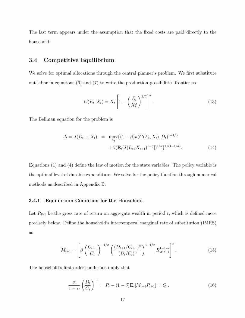
The last term appears under the assumption that the fixed costs are paid directly to the

household.

3.4 Competitive Equilibrium

We solve for optimal allocations through the central planner’s problem. We first substitute

out labor in equations (6) and (7) to write the production-possibilities frontier as

C(Et, Xt) = Xt

[1 −

(Et

Xλt

)1/θ]θ

. (13)

The Bellman equation for the problem is

Jt = J(Dt−1, Xt) = maxEt

{(1 − β)u(C(Et, Xt), Dt)1−1/σ

+β(Et[J(Dt, Xt+1)1−γ])1/κ}1/(1−1/σ). (14)

Equations (1) and (4) define the law of motion for the state variables. The policy variable is

the optimal level of durable expenditure. We solve for the policy function through numerical

methods as described in Appendix B.

3.4.1 Equilibrium Condition for the Household

Let RWt be the gross rate of return on aggregate wealth in period t, which is defined more

precisely below. Define the household’s intertemporal marginal rate of substitution (IMRS)

as

Mt+1 =

[β

(Ct+1

Ct

)−1/σ ((Dt+1/Ct+1)

α

(Dt/Ct)α

)1−1/σ

R1−1/κW,t+1

]κ

. (15)

The household’s first-order conditions imply that

α

1 − α

(Dt

Ct

)−1

= Pt − (1 − δ)Et[Mt+1Pt+1] = Qt. (16)

17

Intuitively, the marginal rate of substitution between the durable and the nondurable good

must equal the user cost of the service flow for the durable good, denoted by Qt. The

user cost is equal to the purchase price today minus the present discounted value of the

depreciated stock tomorrow.

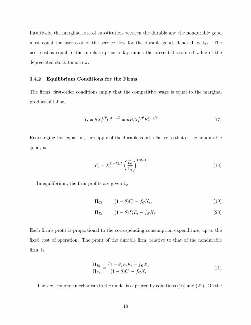
3.4.2 Equilibrium Conditions for the Firms

The firms’ first-order conditions imply that the competitive wage is equal to the marginal

product of labor,

Yt = θX1/θt C

1−1/θt = θPtX

λ/θt E

1−1/θt . (17)

Rearranging this equation, the supply of the durable good, relative to that of the nondurable

good, is

Pt = X(1−λ)/θt

(Et

Ct

)1/θ−1

. (18)

In equilibrium, the firm profits are given by

ΠCt = (1 − θ)Ct − fCXt, (19)

ΠEt = (1 − θ)PtEt − fEXt. (20)

Each firm’s profit is proportional to the corresponding consumption expenditure, up to the

fixed cost of operation. The profit of the durable firm, relative to that of the nondurable

firm, is

ΠEt

ΠCt

=(1 − θ)PtEt − fEXt

(1 − θ)Ct − fCXt

. (21)

The key economic mechanism in the model is captured by equations (16) and (21). On the

18

one hand, equation (16) shows that the household smoothes the ratio the stock of durables

to nondurable consumption. On the other hand, equation (21) shows that the profit of

the durable firm, relative to that of the nondurable firm, is proportional to the ratio of the

expenditure on durables to nondurable consumption. Consequently, the profits of the durable

firm are more volatile than those of the nondurable firm because a proportional change in

the durable stock requires a much larger proportional change in its expenditure.

3.5 Equilibrium Asset Prices

Let VCt be the value of a claim to the profits of the nondurable firm, or the present discounted

value of the stream {ΠC,t+s}∞s=1. The one-period return on the claim is

RC,t+1 =VC,t+1 + ΠC,t+1

VCt

. (22)

In analogous notation, the one-period return on a claim to the profits of the durable firm is

RE,t+1 =VE,t+1 + ΠE,t+1

VEt

. (23)

Let VMt be the value of a claim to total consumption expenditure, or the present dis-

counted value of the stream {Ct+s + Pt+sEt+s}∞s=1. The one-period return on the claim

is

RM,t+1 =VM,t+1 + Ct+1 + Pt+1Et+1

VMt

. (24)

The one-period return on the “wealth portfolio” that enters the IMRS (15) is then given by

RW,t+1 =

(1 − QtDt

VMt + PtDt

)−1(VM,t+1 + Pt+1Dt+1 + Ct+1

VMt + PtDt

). (25)

If the durable good fully depreciates each period (i.e., δ = 1), the durable stock does not

19

enter the wealth portfolio. In this special case, the wealth portfolio collapses to the claim

on total consumption expenditure (i.e., RWt = RMt).

The absence of arbitrage implies that the one-period return on any asset i satisfies

Et[Mt+1Ri,t+1] = 1, (26)

where the IMRS is given by equation (15). In particular, the one-period riskfree interest rate

satisfies

Rf,t+1 =1

Et[Mt+1]. (27)

We use the solution to the planner’s problem and numerical methods to compute asset prices

as described in Appendix B.

3.6 Discussion

Our model is designed to focus on durability as the sole economic mechanism that drives

cross-sectional differences in profits and expected returns. For emphasis, we state this point

formally as a proposition.

Proposition 1. In the special case δ = 1, the profit of the durable firm is a constant

proportion of that of the nondurable firm. Consequently, the two firms have identical rates

of return (i.e., RCt = REt).

Proof. When δ = 1, the household’s first-order condition (16) simplifies to

α

1 − α

(Et

Ct

)−1

= Pt.

Substituting this expression in equation (21),

ΠEt

ΠCt

=α

1 − α.

20

The proposition immediately implies that, in the general case δ < 1, any differences in the

firms’ profits and returns arise from durability alone. The result might initially be surprising

because the productivity of the durable firm is more cyclical than that of the nondurable

firm when λ > 1. The explanation is that the profit of the durable firm also depends on

the relative price of durables, which is endogenously determined through optimal resource

allocation.

Because durability is the only source of asymmetry between the firms, our model provides

a laboratory for assessing the importance of durability as a mechanism for generating cross-

sectional differences in cash flows and returns. The ability to analyze durability in the absence

of asymmetries in preferences or technologies is an advantage of the production approach. In

contrast, the endowment model requires exogenous assumptions about the firms’ cash flows.

Of course, the ability to pinpoint the empirical properties of cash flows is an advantage of the

endowment approach, which makes it especially suitable for matching the key asset-pricing

facts. We refer to Piazzesi, Schneider, and Tuzel (2006) and Yogo (2006) for an analysis of

the endowment model.

4 Quantitative Implications of the Model

4.1 Choice of Parameters

Panel A of Table 7 reports the four macroeconomic quantities that we target in the calibra-

tion. These quantities are

• the log growth rate of real nondurable consumption, log(Ct/Ct−1);

• the log growth rate of real durable expenditure, log(Et/Et−1);

• the ratio of durable expenditure to its stock, Et/Dt;

21

• the ratio of durable expenditure to nondurable consumption, PtEt/Ct.

By matching the first two moments and the autocorrelation for these quantities, we ensure

realistic implications for aggregate consumption and the relative price. We compute the

population moments by simulating the model at annual frequency for 500,000 years.

For the purposes of calibration, “nondurable consumption” in the model is matched to

nondurable and service consumption in the data. Similarly, the “nondurable firm” in the

model is matched to the combination of the nondurable and the service portfolio in the data.

We report the empirical moments for two sample periods, 1930–2004 and 1951–2004. Both

nondurable consumption and durable expenditure are somewhat more volatile in the longer

sample, but otherwise, the empirical moments are quite similar across the samples. We

calibrate to the longer sample because it is a somewhat easier target from the perspective of

explaining asset prices.

As with most general equilibrium models, especially those with production, our model

cannot completely resolve the equity premium and volatility puzzles. Because a quantitative

resolution of these classic issues is attempted elsewhere our focus is on the cross-sectional

findings discussed above.

Table 6 reports the parameters in our benchmark calibration. We set the depreciation

rate to 22%, which matches the value reported by the Bureau of Economic Analysis (BEA)

for consumer durables. We set the growth rate of technology to 2% in order to match the

growth rate of real nondurable consumption. We set the relative productivity of the durable

sector to λ = 1.8 in order to match the growth rate of real durable expenditure. We set

labor elasticity, which is approximately the labor share of aggregate output in the model, to

θ = 0.7 and perform sensitivity analysis around that value.

Following Bansal and Yaron (2004) we model productivity growth as having a persistent

component with an autoregressive parameter φ = 0.78. We choose the standard deviation

22

of the shocks so that log(Xt+1/Xt) has the moments

SD =

(σ2

ε +σ2

ν

1 − φ2

)1/2

= 3%,

Autocorrel =φ

1 + σ2ε (1 − φ2)/σ2

ν

= 0.4.

To generate a nontrivial equity premium, we choose a fairly high risk aversion of γ = 10.

At the same time, we choose a fairly high EIS of σ = 2, which helps keep both the mean

and the volatility of the riskfree rate low. An EIS greater than one also implies that the

substitution effect dominates the income effect, so that asset prices rise in response to a

positive productivity shock. This helps magnify both the equity premium and the volatility

of asset returns. Finally, the intratemporal first-order condition (16) requires that α = 0.12

to pin down the level of durable expenditure relative to nondurable consumption.

4.2 Calibration to Aggregate Consumption

Panel A of Table 7 shows that our choice of parameters leads to a realistic match of the

targeted quantities. We match the mean, the standard deviation, and the autocorrelation

of nondurable consumption growth. We do the same for durable expenditure, except that

the standard deviation is somewhat lower than the empirical counterpart. The standard

deviation of durable expenditure growth is 13% in the full sample and 8% in the model.

A higher value of labor elasticity can raise the spread in volatility between nondurable

consumption and durable expenditure, by making it easier to transfer resources between the

nondurable and durable sectors. However, this channel cannot fully account for the relatively

high volatility of durable expenditure.

Figure 3 shows the optimal policy for the planner’s problem under the benchmark pa-

rameters. We plot policy functions for a state with high productivity growth when εt = σε,

and a state with low productivity growth when εt = −σε. Panel A shows that labor allocated

to the production of durables rises in the productivity shock, holding the existing stock of

23

durables constant. In response to a positive productivity shock, the expenditure on durables

rises (in Panel B) and the relative price of durables falls (in Panel C). These policy functions

verify the simple intuition that the expenditure on durables is more volatile and cyclical

than that on nondurables.

Panel A also shows that labor allocated to the production of durables falls in the existing

stock of durables, holding the productivity growth constant. Intuitively, the household has

little need for additional durables when the existing stock, and hence its service flow, is

already high. Both the expenditure on durables (in Panel B) and the user cost of durables

(in Panel D) are more volatile when the stock of durables is relatively high. If we rearrange

the accumulation equation (1) and compute the conditional variance of both sides,

Dt−1

Et−1

=σt−1(Et/Et−1)

σt−1(Dt/Dt−1). (28)

This relationship between the stock of durables and the conditional volatility of durable

expenditure is a natural consequence of durability. A negative productivity shock causes the

desired future service flow from durables to fall, which is accomplished through a reduction

in the expenditure on new durables. When the existing stock is relatively high, such a

reduction must be more pronounced.

4.3 Calibration to Profits

In our discussion of parameters above, we have deliberately omitted the fixed cost of oper-

ation. This is because the parameter has no bearing on the planner’s problem, and conse-

quently, any of the quantities reported in Panel A of Table 7. We now set this parameter

to f = 0.22 in order to calibrate the model to the volatility of profits. Our empirical proxy

for profits is operating income, which is sales minus the cost of goods sold. Data on sales

and the cost of goods sold, which includes wages and salaries, are from Compustat and are

available only for the postwar sample. In both the model and the data, the market portfolio

24

is the combination of the nondurable and the durable firm.

Panel B of Table 7 reports the mean and the standard deviation of profit growth. Our

simple model of operating leverage introduces a realistic wedge between the volatility of

consumption expenditures and profits. For the nondurable firm, the standard deviation of

profit growth is 3% in the model and 5% in the data. For the durable firm, the standard

deviation of profit growth is 15% in the model and 13% in the data.

4.4 Asset Returns

Equity is a leveraged claim on the firm’s profits. In order to compare firm returns in the

model to stock returns in the data, we must first introduce financial leverage. Consider a

portfolio that is long Vit dollars in firm i and short bVit dollars in the riskfree asset. The

one-period return on the leveraged strategy is

Rit =1

1 − bRit − b

1 − bRft.

In the model, we compute stock returns in this way using an empirically realistic leverage

ratio. We compute the leverage ratio for all Compustat firms as the ratio of the book value

of liabilities to the market value of assets (i.e., the sum of book liabilities and market equity).

While the leverage ratio varies over time, it is on average 52% in the postwar sample. We

therefore set b = 52% in the calibration.

In Panel C of Table 7, we report the first two moments of asset returns implied by the

model. The nondurable firm has excess returns (over the riskfree rate) with mean of 6.75%

and a standard deviation of 10.08%. The durable firm has excess returns with mean of 9.13%

and a standard deviation of 13.67%. The spread in average returns between the two firms

is more than 2%, which is comparable to the empirical counterpart. However, the spread in

the volatility of returns is somewhat lower than the empirical counterpart because our model

is not designed to resolve the equity volatility puzzle. The riskfree rate is 0.96% on average

25

with low volatility, consistent with empirical evidence. Overall, the model supports the key

empirical facts, that the durable portfolio has returns that are higher on average and more

volatile.

4.5 Predictability of Returns

We use the calibrated model to simulate 10,000 samples, each consisting of 50 annual ob-

servations. In each sample, we run a regression of excess returns onto the lagged durable

expenditure-stock ratio. Panel A of Table 8 reports the mean and the standard deviation of

the t-statistic from the regression across the simulated samples. The goal of this exercise is

to see whether the model replicates the evidence for predictability in actual data, reported

in Panel A of Table 4. The regression coefficient is negative for both firms, and the t-statistic

for the durable firm is larger than that for the nondurable firm. This pattern is consistent

with the empirical evidence, especially accounting for the moderate sampling variance.

In Panel B, we use the simulated data to run a regression of absolute excess returns onto

the lagged durable expenditure-stock ratio. The regression coefficient is negative for both

firms, and the t-statistic for the durable firm is larger than that for the nondurable firm.

This pattern is consistent with the empirical evidence presented in Panel B of Table 4.

In Panel C, we use the simulated data to run a regression of absolute profit growth

onto the lagged durable expenditure-stock ratio. The regression coefficient is positive for

the nondurable firm and negative for the durable firm. This pattern is consistent with the

empirical evidence presented in Table 5.

To understand these simulation results, it is helpful to distinguish two sources of pre-

dictability in the model. The first source is the common component that is responsible for

the predictability of the market portfolio. The IMRS (15) depends on the stock of durables

as a ratio of nondurable consumption, which is proportional to the user cost of durables

through the household’s intratemporal first-order condition (16). As shown in Panel D of

Figure 3, the user cost of durables is more volatile when the stock of durables is relatively

26

high. This implies that the IMRS is more volatile when the stock of durables is relatively

high.

The second source is the independent component that is responsible for the predictability

of the durable firm above and beyond that of the nondurable firm. Figure 4 shows the profits

and the value (i.e., the present discounted value of profits) of both firms as a function of the

existing stock of durables. The profits of the durable firm (in Panel B) is more sensitive to

aggregate productivity shocks when the stock of durables is relatively high, in contrast to

the profits of the nondurable firm (in Panel A). In other words, the conditional volatility of

the profits of the durable firm rises in the existing stock of durables. As compensation for

the higher conditional cash-flow risk, the durable firm earns a higher expected return when

the stock of durables is relatively high.

4.6 Consumption Betas

In order to quantify the sources of risk, Table 9 reports consumption betas for each of

the portfolios. We compute the betas through a regression of excess returns onto the log

growth rate of nondurable consumption, log(Ct/Ct−1), and the log growth rate of durable

stock, log(Dt/Dt−1). The nondurable firm has a nondurable consumption beta of 2.87 and a

durable consumption beta of −1.84. The durable firm has a nondurable consumption beta

of 3.87 and a durable consumption beta of −2.85.

As shown in Figure 4, the profits of the durable firm are more sensitive to aggregate

productivity shocks than those of the nondurable firm, holding the stock of durables constant.

Because nondurable consumption growth is proportional to aggregate productivity growth,

the durable firm has a higher nondurable consumption beta than the nondurable firm.

As shown in Table 8, expected returns are low when the durable expenditure-stock ratio

is high. Through the accumulation equation (1), the growth rate of durable stock, Dt/Dt−1,

is high when the durable expenditure-stock ratio, Et/Dt, is high. Therefore, expected returns

are low when the growth rate of durable stock is high, leading to a negative durable con-

27

sumption beta. Because the durable firm has expected returns that are more time-varying

than those of the nondurable firm, the durable firm has a lower durable consumption beta

than the nondurable firm.

5 Relationship between Risk and Return

This section extends the analysis in Section 2 by further investigating the empirical properties

of portfolios sorted by the durability of output. Specifically, we use a model of risk and return

to show that the durability of output is a priced risk factor in both the cross-section and the

time series of expected returns.

We evaluate portfolio returns with respect to two different factor models. The first is

the Fama-French (1993) three-factor model, in which the factors are excess market returns,

SMB (small minus big market equity) portfolio returns, and HML (high minus low book-to-

market equity) portfolio returns. The second is a consumption-based model, in which the

factors are nondurable and durable consumption growth. The consumption-based model can

be formally motivated as an approximation to the Euler equation (26), as shown in Yogo

(2006, Appendix C). As is well known, the Euler equation holds even in an economy in which

production is different from the particular model described in Section 3. In that sense, the

estimation in this section is more general than the calibration in the last section.

5.1 Cross-Sectional Variation in Expected Returns

5.1.1 Empirical Framework

Let Rit denote the excess return on an asset i in period t. Let “nondurable consumption”

refer to real nondurable and service consumption, where ∆ct denotes its log growth rate. Let

“durable consumption” refer to the real stock of consumer durables, where ∆dt denotes its

log growth rate. We model the cross-sectional relationship between risk and return through

28

a linear factor model,

E[Rit] = b1Cov(Rit, ∆ct) + b2Cov(Rit, ∆dt). (29)

This equation says that the variation in expected returns across assets must reflect the

variation in the quantity of risk across assets, measured by the covariance of returns with

consumption growth. Appendix C contains details on the estimation of the linear factor

model.

The test assets are the three Fama-French factors and the five industry portfolios. For

the industry portfolios, we compute excess returns over the three-month T-bill. We use

quarterly (rather than annual) data for the period 1951:1–2004:4 to obtain more precise

estimates of the covariance between asset returns and consumption growth. Appendix A

contains a detailed description of the consumption data.

5.1.2 Empirical Findings

Panel A of Table 10 reports the annualized excess returns on the eight portfolios. Among

the five industry portfolios, the durable portfolio has the highest excess returns with mean of

8.19%. The service portfolio has the lowest excess returns with mean of 5.66%. The spread

in average excess returns between the durable and the service portfolio is 2.53%, which is

comparable to the size premium of 2.87% in this sample period. The nondurable portfolio

has unusually high excess returns in this sample period with mean of 8.07%. This finding can

be explained by the relatively high returns on energy stocks during the decade 1965–1974

(see Table 3).

In the first column of Table 11, we examine whether the Fama-French three-factor model

explains cross-sectional returns on the eight portfolios. The risk price for the market factor

is 3.24, and the risk price for the HML factor is 2.60. The risk price for the SMB factor is not

significantly different from zero. The R2 is 67%, which suggests that the Fama-French model

29

explains some of the variation in average excess returns. However, the J-test (i.e., the test of

overidentifying restrictions) rejects the model with a p-value of 3%. The rejection highlights

the importance of including industry portfolios in cross-sectional asset pricing tests, which

has been recently emphasized by Lewellen, Nagel, and Shanken (2006).

In the second column of Table 11, we examine whether the consumption-based model

explains cross-sectional returns on the eight portfolios. The risk price for nondurable con-

sumption growth is 22, while the risk price for durable consumption growth is 93. Of the two

risk factors, only durable consumption growth has a risk price that is significantly different

from zero, implying that this factor alone explains most of the variation in average excess

returns. The R2 of the model is 92%, which is higher than that for the Fama-French model.

The J-test fails to reject the model with a p-value of 22%.

In order to better understand the relationship between risk and return, Table 10 reports

the betas and the alphas for the eight portfolios. As shown in Panel C, the service portfolio

has a nondurable consumption beta of 4.79 and a durable consumption beta of −1.01. The

nondurable portfolio has a nondurable consumption beta of 4.01 and a durable consumption

beta of 0.16. The durable portfolio has a nondurable consumption beta of 7.45 and a durable

consumption beta of −1.49. In summary, firms that produce durable goods have a higher

nondurable consumption beta and a lower durable consumption beta than firms that produce

nondurable goods and services. This pattern is precisely that predicted by the model, as

reported in Table 9.

The investment portfolio has the largest alpha with respect to the consumption-based

model. In other words, this portfolio has average returns that are too low relative to their

measured risk. As shown in Panel B, this is also the case with respect to the Fama-French

model. This failure can be partly rationalized by the fact that firms that produce investment

goods, which presumably act as inputs for firms that produce consumption goods, are outside

the scope of our general equilibrium model. A potentially interesting extension of our model

is to incorporate a type of firm that produces investment goods (see Papanikolaou (2006)).

30

5.2 Time Variation in Expected Returns

5.2.1 Empirical Framework

We model the time-series relationship between risk and return through a conditional factor

model,

Et−1[Rit] = b1Covt−1(Rit, ∆ct) + b2Covt−1(Rit, ∆dt). (30)

This equation says that the variation in expected returns over time must reflect the variation

in the quantity of risk over time, measured by the conditional covariance of returns with

consumption growth.

Following the approach in Campbell (1987) and Harvey (1989), we model the conditional

moments in equation (30) as linear functions of a vector of instruments xt−1, observed at

t − 1. For a set of assets indexed by i, we estimate the linear regression model

Rit = Π′ixt−1 + εit, (31)

εit∆ct = Υ′i1xt−1 + ηi1t, (32)

εit∆dt = Υ′i2xt−1 + ηi2t. (33)

The conditional factor model (30) implies cross-equation restrictions of the form

Πi = b1Υi1 + b2Υi2. (34)

Appendix C contains further details on estimation of the conditional factor model.

Our estimation is based on four excess returns and three instruments. The excess re-

turns are the market portfolio over the three-month T-bill and each of the PCE (service,

nondurable, and durable) portfolios over the market portfolio. The instruments are the

durable expenditure-stock ratio, the dividend yield for the market portfolio, and a constant.

31

In the estimation, we impose the risk prices b1 = 22 and b2 = 93, which are the estimated

risk prices from Table 11. This procedure ensures that the asset-pricing implications for the

time series are consistent with those for the cross-section.

5.2.2 Empirical Findings

Panel A of Table 12 reports estimates of the regression model (31) for the conditional mean

of excess returns. The estimates imply that the durable expenditure-stock ratio is the key

instrument that explains time variation in expected returns. The estimated coefficient is

−0.20 for excess returns on the market portfolio. Because the durable expenditure-stock ratio

is procyclical, the negative coefficient implies that the equity premium is countercyclical.

The estimated coefficient is 0.03 for excess returns on the service portfolio over the market

portfolio. The positive coefficient implies that the expected return on the service portfolio

is less cyclical than that on the market portfolio. In contrast, the estimated coefficient is

−0.07 for excess returns on the durable portfolio over the market portfolio. The negative

coefficient implies that the expected return on the durable portfolio is more cyclical than

that on the market portfolio. Between these two extremes is the expected return on the

nondurable portfolio, which is slightly more cyclical than the market portfolio.

In Panels B and C, we investigate whether the cyclical variation in expected returns

is matched by cyclical variation in risk, measured by the conditional covariance of returns

with consumption growth. In particular, Panel C reports estimates of the regression model

(33) for the conditional covariance of returns with durable consumption growth. The durable

expenditure-stock ratio predicts the product of the innovations to market return and durable

consumption growth with a coefficient of −0.21. Because the durable expenditure-stock ratio

is procyclical, the negative coefficient implies that the conditional covariance of the market

return with durable consumption growth is countercyclical.

The estimated coefficient is 0.03 for excess returns on the service portfolio over the market

portfolio. The positive coefficient implies that the conditional covariance for the service

32

portfolio is less cyclical than that for the market portfolio. In contrast, the estimated

coefficient is −0.08 for excess returns on the durable portfolio over the market portfolio.

The negative coefficient implies the conditional covariance for the durable portfolio is more

cyclical than that for the market portfolio.

Panel B of Figure 2 is a visual representation of the results in Table 12. The figure shows

a time-series plot of expected excess market returns (i.e., the equity premium), implied by

the estimates in Table 12. The heavy line represents the total equity premium, Et−1[Rit],

and the light line represents the part due to durable consumption, b2Covt−1(Rit, ∆dt). The

difference between the two lines is the premium due to nondurable consumption. The plot

reveals two interesting facts. First, the equity premium is strongly countercyclical, that is,

highest at business-cycle troughs and lowest at peaks. Second, the two lines move closely

together, which implies that most of the time variation in the equity premium is driven by

the time variation in durable consumption risk.

Figure 5 shows the premium on the service, the nondurable, and the durable portfolio

over the market portfolio. A portfolio strategy that is long on the service portfolio and short

on the market portfolio has procyclical expected returns. For example, expected returns are

low during the 1960:2–1961:3 and 1980:1–1982:4 recessions. In contrast, a portfolio strategy

that is long on the durable portfolio and short on the market portfolio has countercyclical

expected returns. For example, expected returns are high during the same two recessions.

In summary, Table 12 uncovers a new empirical fact that the premium on the service

portfolio is less cyclical, and the premium on the durable portfolio is more cyclical than that

on the market portfolio. The countercyclical variation in expected returns is matched by

countercyclical variation in the quantity of risk, as captured by the conditional covariance of

returns with durable consumption growth. Durable stocks deliver unexpectedly low returns

during recessions when durable consumption growth is low. Therefore, investors demand a

higher premium for holding durable stocks during recessions, above and beyond the usual

compensation for stock market risk.

33

6 Conclusion

The literature on the cross-section of stock returns has documented a number empirical

relationships between characteristics and expected returns. Although these studies provide

useful descriptions of stock market data, they provide a limited insight into the underlying

economic determinants of stock returns. Consequently, proposed explanations for these

empirical findings represent a broad spectrum of ideologies, which include compensation

for yet undiscovered economic risk factors (Fama and French 1993), investor mistakes (De

Bondt and Thaler 1985, Lakonishok, Shleifer, and Vishny 1994), and data snooping (Lo

and MacKinlay 1990). A more fruitful approach to the study of stock returns is to find

direct empirical relationships between sources of systematic risk and expected returns. For

instance, Pastor and Stambaugh (2003) find evidence that aggregate liquidity risk is priced

in the cross-section of stock returns.

Ultimately, prices should not be viewed as characteristics by which to rationalize differ-

ences in expected returns. Instead, prices and expected returns should jointly be explained

by more fundamental aspects of firm heterogeneity, such as the demand for their output. In

this paper, we have shown that durability is an important aspect of demand that is priced

in the cross-section of stock returns. Firms that produce durable goods have higher average

returns, and their expected returns vary more over the business cycle. We suspect that

there are other, and perhaps more important, aspects of demand that explain differences in

expected returns.

34

Appendix A Consumption Data

We work with two samples of consumption data: a longer annual sample for the period

1930–2004 and a shorter quarterly sample for the period 1951:1–2004:4. We construct our

data using the following tables from the BEA.

• NIPA Table 2.3.4: Price Indexes for Personal Consumption Expenditures by Major

Type of Product.

• NIPA Table 2.3.5: Personal Consumption Expenditures by Major Type of Product.

• NIPA Table 7.1: Selected Per Capita Product and Income Series in Current and

Chained Dollars.

• Fixed Assets Table 8.1: Current-Cost Net Stock of Consumer Durable Goods.

Nondurable consumption is the properly chain-weighted sum of real PCE on nondurable

goods and real PCE on services. The data for the stock of durable goods are available only

at annual frequency (measured at each year end). We therefore construct a quarterly series

that is consistent with the accumulation equation (1), using quarterly data for real PCE on

durable goods. The depreciation rate for durable goods, implied by the construction, is about

6% per quarter. In computing growth rates, we divide all quantities by the population. In

matching consumption growth to returns at the quarterly frequency, we use the “beginning-

of-period” timing convention as in Campbell (2003).

To deflate asset returns and cash-flow growth, we use the consumer price index (CPI) for

all urban consumers from the Bureau of Labor Analysis. The CPI is the only consistent time

series for consumer prices going back to 1926, which is the beginning of the CRSP database.

The CPI is based on a basket of goods and services from eight major groups of expenditures:

food and beverages; housing; apparel; transportation; medical care; recreation; education

and communication; and other nondurable goods and services. Because the CPI measures

35

the price of nondurable goods and services, our deflating methodology is consistent with our

modeling convention that the nondurable good is the numeraire in the economy.

Appendix B Numerical Solution of the Model

B.1 Central Planner’s Problem

We first rescale all variables by the appropriate power of aggregate productivity to make the

planner’s problem stationary. We define the rescaled value function Jt = Jt/X1+α(λ−1)t . We

also define the rescaled variables Ct = Ct/Xt, Et = Et/Xλt , Dt = Dt/X

λt , and Pt = Pt/X

1−λt .

Let ∆Xt+1 = Xt+1/Xt. By homotheticity, we can solve an equivalent problem defined by

the Bellman equation

Jt = J(Dt−1, ∆Xt) = maxEt

{(1 − β)u(C(Et), Dt)1−1/σ

+β(Et[∆X(1−γ)(1+α(λ−1))t+1 J(Dt, ∆Xt+1)

1−γ])1/κ}1/(1−1/σ), (B1)

C(Et) = (1 − E1/θt )θ. (B2)

The law of motion for the state variables are given by

Dt = (1 − δ)Dt−1

∆Xλt

+ Et (B3)

and equation (4).

We discretize the state space and solve the dynamic program through policy iteration.

We start with an initial guess that the user cost is Qt = δPt. Then the intratemporal

first-order condition (16) implies that

α

1 − α

(Dt

Ct

)−1

= δPt. (B4)

36

Our initial guess of the policy function, Et = E(Dt−1, ∆Xt), is the solution to the system of

three nonlinear equations (18), (B2), and (B4). We then use the following recursion to solve

the problem.

1. Compute the value function Ji corresponding to the current policy function Ei.

2. Update the policy function Ei+1, using Ji and the intratemporal first-order condition

(16).

3. If ‖Ei+1 − Ei‖ is less than the convergence criteria, stop. Otherwise, return to step 1.

B.2 Asset Prices

As shown by Yogo (2006, Appendix B), the value of the claim to total consumption expen-

diture is related to the value function (14) through the equation

VMt =C

1/σt (Dt/Ct)

α(1/σ−1)J1−1/σt

(1 − β)(1 − α)− Ct − PtDt. (B5)

We use the solution to the planner’s problem to compute the return on the wealth portfolio

(25) and the IMRS (15). We then solve for the (rescaled) value of the two firms by iterating

on the Euler equations

VCt = VC(Dt−1, ∆Xt) = Et[Mt+1∆Xt+1(VC(Dt, ∆Xt+1) + ΠC,t+1)], (B6)

VEt = VE(Dt−1, ∆Xt) = Et[Mt+1∆Xt+1(VE(Dt, ∆Xt+1) + ΠE,t+1)]. (B7)

We compute the riskfree rate through equation (27).

37

Appendix C Estimating the Relationship between Risk

and Return

We use the following notation throughout this appendix. The vector Rt = (R1t, . . . , RNt)′

denotes the time t observation on N excess returns with mean µR and covariance matrix ΣR.

The vector ft = (f1t, . . . , fFt)′ denotes the time t observation on F factors with mean µf and

covariance matrix Σf . The vector xt denotes the time t observation on I instruments. For

any parameter vector θ, the symbol θ denotes a corresponding consistent estimator.

C.1 Cross-Sectional Estimation

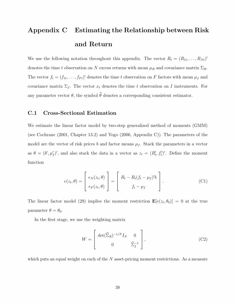
We estimate the linear factor model by two-step generalized method of moments (GMM)

(see Cochrane (2001, Chapter 13.2) and Yogo (2006, Appendix C)). The parameters of the

model are the vector of risk prices b and factor means µf . Stack the parameters in a vector

as θ = (b′, µ′f )

′, and also stack the data in a vector as zt = (R′t, f

′t)

′. Define the moment

function

e(zt, θ) =

⎡⎢⎣ eN(zt, θ)

eF (zt, θ)

⎤⎥⎦ =

⎡⎢⎣ Rt − Rt(ft − µf )′b

ft − µf

⎤⎥⎦ . (C1)

The linear factor model (29) implies the moment restriction E[e(zt, θ0)] = 0 at the true

parameter θ = θ0.

In the first stage, we use the weighting matrix

W =

⎡⎢⎣ det(ΣR)−1/NIN 0

0 Σ−1f

⎤⎥⎦ , (C2)

which puts an equal weight on each of the N asset-pricing moment restrictions. As a measure

38

of first-stage fit, we compute the statistic

R2 = 1 − ‖∑t eN(zt, θ)‖2

‖∑t(Rt − µR)‖2. (C3)

We compute heteroskedasticity- and autocorrelation-consistent (HAC) standard errors through

the VARHAC procedure with automatic lag length selection by the Akaike information cri-

teria (see Den Haan and Levin (1997)).

C.2 Time-Series Estimation

We estimate the conditional factor model by two-step GMM (see Yogo (2006, Appendix D)).

The linear regression model (31)–(33), in more compact notation, is

Rit = Π′ixt−1 + εit (i = 1, . . . , N), (C4)

εitfjt = Υ′ijxt−1 + ηijt (i = 1, . . . , N ; j = 1, . . . , F ). (C5)

The parameters of the model are the vector of risk prices b and the conditional covariance

matrices

Υj = [Υ1j · · ·ΥNj] (I × N), (C6)

Υ = [Υ1 · · ·ΥF ] (I × NF ). (C7)

Stack the parameters in a vector as θ = (b′, vec(Υ)′)′, and also stack the data in a vector as

zt = (R′t, f

′t , x

′t−1)

′. Define the moment function

e(zt, θ) =

⎡⎢⎣ Rt − (∑F

j=1 bjΥj)′xt−1

vec([Rt − (∑F

j=1 bjΥj)′xt−1]f

′t) − Υ′xt−1

⎤⎥⎦⊗ xt−1. (C8)

39

The conditional factor model (30) implies the moment restriction E[e(zt, θ0)] = 0 at the true

parameter θ = θ0.

40

References

Bansal, Ravi, and Amir Yaron, 2004, Risks for the long run: A potential resolution of asset

pricing puzzles, Journal of Finance 59, 1481–1509.

Banz, Rolf W., 1981, The relationship between return and market value of common stocks,

Journal of Financial Economics 9, 3–18.

Basu, Sanjoy, 1983, The relationship between earnings yield, market value, and return for

NYSE common stocks: Further evidence, Journal of Financial Economics 12, 129–156.

Berk, Jonathan B., Richard C. Green, and Vasant Naik, 1999, Optimal investment, growth

options, and security returns, Journal of Finance 54, 1153–1607.

Bhandari, Laxmi Chand, 1988, Debt/equity ratio and expected common stock returns: Em-

pirical evidence, Journal of Finance 43, 507–528.

Bils, Mark, and Peter J. Klenow, 1998, Using consumer theory to test competing business

cycle models, Journal of Political Economy 106, 233–261.

Black, Fischer, Michael C. Jensen, and Myron Scholes, 1972, The capital asset pricing model:

Some empirical tests, in Michael C. Jensen, ed.: Studies in Theory of Capital Markets

(Preager: New York).

Boudoukh, Jacob, Roni Michaely, Matthew Richardson, and Michael R. Roberts, 2007, On

the importance of measuring payout yield: Implications for empirical asset pricing, Journal

of Finance 62, forthcoming.

Breeden, Douglas T., Michael R. Gibbons, and Robert H. Litzenberger, 1989, Empirical test

of the consumption-oriented CAPM, Journal of Finance 44, 231–262.

Bureau of Economic Analysis, 1994, Benchmark input-output accounts for the U.S. economy,

1987, Survey of Current Business 4, 73–115.

41

Campbell, John Y., 1987, Stock returns and the term structure, Journal of Financial Eco-

nomics 18, 373–399.

Campbell, John Y., 1991, A variance decomposition for stock returns, Economic Journal

101, 157–179.

Campbell, John Y., 2003, Consumption-based asset pricing, in George M. Constantinides,

Milton Harris, and Rene M. Stulz, ed.: Handbook of the Economics of Finance, vol. 1B .

chap. 13, pp. 801–885 (Elsevier: Amsterdam).

Campbell, John Y., and John H. Cochrane, 1999, By force of habit: A consumption-based

explanation of aggregate stock market behavior, Journal of Political Economy 107, 205–

251.

Carlson, Murray, Adlai Fisher, and Ron Giammarino, 2004, Corporate investment and asset

price dynamics: Implications for the cross-section of returns, Journal of Finance 59, 2577–

2603.

Cochrane, John H., 1991, Production-based asset pricing and the link between stock returns

and economic fluctuations, Journal of Finance 46, 209–237.

Cochrane, John H., 2001, Asset Pricing (Princeton University Press: Princeton, NJ).

Davis, James L., Eugene F. Fama, and Kenneth R. French, 2000, Characteristics, covariances,

and average returns: 1929 to 1997, Journal of Finance 55, 389–406.

De Bondt, Werner F. M., and Richard Thaler, 1985, Does the stock market overreact?,

Journal of Finance 40, 793–805.

Den Haan, Wouter J., and Andrew T. Levin, 1997, A practitioner’s guide to robust covariance

matrix estimation, in G.S. Maddala, and C.R. Rao, ed.: Handbook of Statistics, vol. 15 .

pp. 299–342 (Elsevier: Amsterdam).

42

Dunn, Kenneth B., and Kenneth J. Singleton, 1986, Modeling the term structure of interest

rates under non-separable utility and durability of goods, Journal of Financial Economics

17, 27–55.

Eichenbaum, Martin, and Lars Peter Hansen, 1990, Estimating models with intertemporal

substitution using aggregate time series data, Journal of Business and Economic Statistics

8, 53–69.

Epstein, Larry G., and Stanley E. Zin, 1991, Substitution, risk aversion, and the temporal

behavior of consumption and asset returns: An empirical analysis, Journal of Political

Economy 99, 263–286.

Fama, Eugene F., and Kenneth R. French, 1992, The cross-section of expected stock returns,

Journal of Finance 47, 427–465.

Fama, Eugene F., and Kenneth R. French, 1993, Common risk factors in the returns on

stocks and bonds, Journal of Financial Economics 33, 3–56.

Fama, Eugene F., and James D. MacBeth, 1973, Risk, return, and equilibrium: Empirical

tests, Journal of Political Economy 81, 607–636.

Gala, Vito D., 2006, Investment and returns, Working paper, London Business School.

Gomes, Joao, Leonid Kogan, and Lu Zhang, 2003, Equilibrium cross section of returns,

Journal of Political Economy 111, 693–732.

Gomes, Joao F., Leonid Kogan, and Motohiro Yogo, 2006, Data appendix for ‘Durability of

output and expected stock returns’, Working paper, University of Pennsylvania.

Gourio, Francois, 2005, Operating leverage, stock market cyclicality, and the cross section

of returns, Working paper, Boston University.

Harvey, Campbell R., 1989, Time-varying conditional covariances in tests of asset pricing

models, Journal of Financial Economics 24, 289–317.

43

Jegadeesh, Narasimhan, and Sheridan Titman, 1993, Returns to buying winners and selling

losers: Implications for stock market efficiency, Journal of Finance 48, 65–91.

Kogan, Leonid, 2001, An equilibrium model of irreversible investment, Journal of Financial

Economics 62, 201–245.

Kogan, Leonid, 2004, Asset prices and real investment, Journal of Financial Economics 73,

411–431.

Lakonishok, Josef, Andrei Shleifer, and Robert W. Vishny, 1994, Contrarian investment,

extrapolation, and risk, Journal of Finance 49, 1541–78.

Lamont, Owen A., 2001, Economic tracking portfolios, Journal of Econometrics 105, 161–

184.

Lewellen, Jonathan, Stefan Nagel, and Jay Shanken, 2006, A skeptical appraisal of asset

pricing tests, Working paper, Dartmouth University.

Lo, Andrew W., and A. Craig MacKinlay, 1990, Data-snooping biases in tests of financial

asset pricing models, Review of Financial Studies 3, 431–467.

Ogaki, Masao, and Carmen M. Reinhart, 1998, Measuring intertemporal substitution: The

role of durable goods, Journal of Political Economy 106, 1078–1098.

Pakos, Michal, 2004, Asset pricing with durable goods and non-homothetic preferences,

Working paper, Carnegie Mellon University.

Papanikolaou, Dimitris, 2006, Investment technology shocks and asset prices, Working paper,

MIT.

Pastor, Lubos, and Robert F. Stambaugh, 2003, Liquidity risk and expected stock returns,

Journal of Political Economy 111, 642–685.

44

Petersen, Bruce, and Steven Strongin, 1996, Why are some industries more cyclical than

others?, Journal of Business and Economic Statistics 14, 189–198.

Piazzesi, Monika, Martin Schneider, and Selale Tuzel, 2006, Housing, consumption and asset

pricing, Working paper, University of Chicago.

Rosenberg, Barr, Kenneth Reid, and Ronald Lanstein, 1985, Persuasive evidence of market

inefficiency, Journal of Portfolio Management 11, 9–17.

Shiller, Robert J., 1993, Macro Markets . Clarendon Lectures in Economics (Oxford Univer-

sity Press: New York).

Tuzel, Selale, 2005, Corporate real estate holdings and the cross section of stock returns,

Working paper, University of Southern California.

Yogo, Motohiro, 2006, A consumption-based explanation of expected stock returns, Journal

of Finance 61, 539–580.

Zhang, Lu, 2006, Anomalies, Working paper, University of Michigan.

45

Table 1: Properties of the PCE PortfoliosWe sort NYSE, AMEX, and Nasdaq stocks into five industry portfolios based on their SICcodes. The industries are defined by their primary contribution to final demand accordingto the NIPA input-output tables. We compute portfolio properties in December of each yearand report the time-series average over the indicated sample period. The reported propertiesare the number of firms in each portfolio, the share of total market equity that each portfoliorepresents, log dividend yield, log book-to-market equity, and log liabilities-to-market equity.

Variable Services Nondurables Durables Investment OtherPanel A: Sample Period 1927–2004

Number of Firms 415 401 189 638 1175Share of Market Equity (%) 14.6 35.3 15.9 16.7 17.5Dividend Yield -2.97 -3.12 -3.04 -3.29 -3.24

Panel B: Sample Period 1951–2004Number of Firms 547 493 233 844 1616Share of Market Equity (%) 10.2 39.2 15.6 17.2 17.8Dividend Yield -3.01 -3.18 -3.09 -3.42 -3.34Book-to-Market Equity -0.24 -0.71 -0.52 -0.63 -0.58Liabilities-to-Market Equity 0.07 -0.82 -0.13 -0.62 0.63

Table 2: Sales and Operating Income for the PCE PortfoliosThe table reports descriptive statistics for the log annual growth rate of sales and operatingincome for the PCE portfolios. Operating income is sales minus the cost of goods sold.Correlation is with the log growth rate of real service consumption, nondurable consumption,and durable expenditure. Data on sales and the cost of goods sold are from Compustat andare deflated by the CPI. The sample period is 1951–2004.

Statistic Services Nondurables DurablesPanel A: Sales

Mean (%) 5.62 4.54 3.15Standard Deviation (%) 5.94 5.43 8.16Correlation with the Growth of

Service Consumption 0.13 -0.01 0.62Nondurable Consumption 0.19 0.04 0.49Durable Expenditure 0.07 -0.10 0.81

Panel B: Operating IncomeMean (%) 5.36 4.70 3.00Standard Deviation (%) 5.99 5.55 12.77Correlation with the Growth of

Service Consumption 0.25 0.27 0.60Nondurable Consumption 0.20 0.31 0.39Durable Expenditure 0.29 0.33 0.79

46

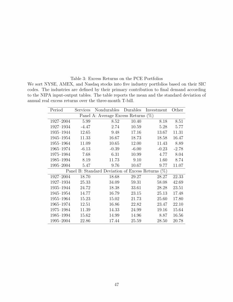
Table 3: Excess Returns on the PCE PortfoliosWe sort NYSE, AMEX, and Nasdaq stocks into five industry portfolios based on their SICcodes. The industries are defined by their primary contribution to final demand accordingto the NIPA input-output tables. The table reports the mean and the standard deviation ofannual real excess returns over the three-month T-bill.

Period Services Nondurables Durables Investment OtherPanel A: Average Excess Returns (%)

1927–2004 5.99 8.52 10.40 8.18 8.511927–1934 -4.47 2.74 10.59 5.28 5.771935–1944 12.65 9.48 17.16 13.67 11.311945–1954 11.33 16.67 18.73 18.58 16.471955–1964 11.09 10.65 12.00 11.43 8.891965–1974 -6.13 -0.39 -6.00 -0.23 -2.781975–1984 7.68 6.31 10.99 4.77 8.041985–1994 8.19 11.73 9.10 1.60 8.741995–2004 5.47 9.76 10.67 9.77 11.07

Panel B: Standard Deviation of Excess Returns (%)1927–2004 18.70 18.68 29.27 28.27 22.331927–1934 25.33 34.09 59.31 58.08 42.691935–1944 24.72 18.38 33.61 28.28 23.511945–1954 14.77 16.79 23.15 25.13 17.481955–1964 15.23 15.02 21.73 25.60 17.801965–1974 12.51 16.86 22.82 23.47 22.101975–1984 11.39 14.33 24.99 19.16 15.641985–1994 15.62 14.99 14.96 8.87 16.561995–2004 22.86 17.44 25.59 28.50 20.78

47

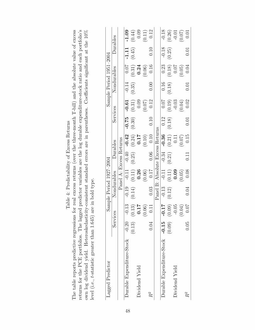
Tab

le4:

Pre

dic

tability

ofE

xce

ssR

eturn

sT

he

table

repor

tspre

dic

tive

regr

essi

ons

for

real

exce

ssre

turn

s(o

ver

the

thre

e-m

onth

T-b

ill)

and

the

abso

lute

valu

eof

exce

ssre

turn

sfo

rth

eP

CE

por

tfol

ios.

The

lagg

edpre

dic

tor

vari

able

sar

eth

elo

gdura

ble

expen

dit

ure

-sto

ckra

tio

and

each

por

tfol

io’s

own

log

div

iden

dyie

ld.

Het

eros

kedas

tici

ty-c

onsi

sten

tst

andar

der

rors

are

inpar

enth

eses

.C

oeffi

cien

tssi

gnifi

cant

atth

e10

%le

vel(i

.e.,

t-st

atis

tic

grea

ter

than

1.64

5)ar

ein

bol

dty

pe.

Lag

ged

Pre

dic

tor

Sam

ple

Per

iod

1927

–200

4Sam

ple

Per

iod

1951

–200

4Ser

vic

esN

ondura

ble

sD

ura

ble

sSer

vic

esN

ondura

ble

sD

ura

ble

sPan

elA

:E

xce

ssR

eturn

sD

ura

ble

Expen

dit

ure

-Sto

ck-0

.20

-0.1

3-0

.19

-0.1

1-0

.40

-0.4

2-0

.75

-0.6

1-0

.14

0.07

-1.1

1-1

.09

(0.1

3)(0

.13)

(0.1

4)(0

.11)

(0.2

5)(0

.24)

(0.3

0)(0

.31)

(0.3

5)(0

.31)

(0.4

5)(0

.44)

Div

iden

dY

ield

0.1

70.2

60.1

70.

090.2

40.

09(0

.06)

(0.0

6)(0

.10)

(0.0

7)(0

.06)

(0.1

1)R

20.

040.

110.

030.

170.

060.

100.

100.

120.

000.

160.

100.

12Pan

elB

:A

bso

lute

Exce

ssR

eturn

sD

ura

ble

Expen

dit

ure

-Sto

ck-0

.15

-0.1

7-0

.13

-0.1

1-0

.34

-0.3

60.

120.

070.

160.

23-0

.18

-0.1

8(0

.09)

(0.0

9)(0

.12)

(0.1

1)(0

.21)

(0.2

1)(0

.18)

(0.1

9)(0

.18)

(0.1

8)(0

.25)

(0.2

6)D

ivid

end

Yie

ld-0

.05

0.0

90.

11-0

.03

0.07

-0.0

1(0

.04)

(0.0

5)(0

.07)

(0.0

4)(0

.05)

(0.0

7)R

20.

050.

070.

040.

080.

110.

150.

010.

020.

010.

040.

010.

01

48

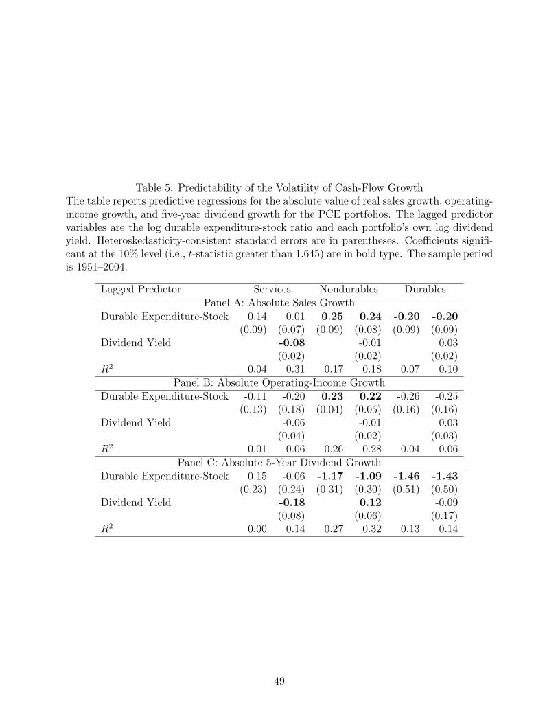
Table 5: Predictability of the Volatility of Cash-Flow GrowthThe table reports predictive regressions for the absolute value of real sales growth, operating-income growth, and five-year dividend growth for the PCE portfolios. The lagged predictorvariables are the log durable expenditure-stock ratio and each portfolio’s own log dividendyield. Heteroskedasticity-consistent standard errors are in parentheses. Coefficients signifi-cant at the 10% level (i.e., t-statistic greater than 1.645) are in bold type. The sample periodis 1951–2004.

Lagged Predictor Services Nondurables DurablesPanel A: Absolute Sales Growth

Durable Expenditure-Stock 0.14 0.01 0.25 0.24 -0.20 -0.20(0.09) (0.07) (0.09) (0.08) (0.09) (0.09)

Dividend Yield -0.08 -0.01 0.03(0.02) (0.02) (0.02)

R2 0.04 0.31 0.17 0.18 0.07 0.10Panel B: Absolute Operating-Income Growth

Durable Expenditure-Stock -0.11 -0.20 0.23 0.22 -0.26 -0.25(0.13) (0.18) (0.04) (0.05) (0.16) (0.16)

Dividend Yield -0.06 -0.01 0.03(0.04) (0.02) (0.03)

R2 0.01 0.06 0.26 0.28 0.04 0.06Panel C: Absolute 5-Year Dividend Growth

Durable Expenditure-Stock 0.15 -0.06 -1.17 -1.09 -1.46 -1.43(0.23) (0.24) (0.31) (0.30) (0.51) (0.50)

Dividend Yield -0.18 0.12 -0.09(0.08) (0.06) (0.17)

R2 0.00 0.14 0.27 0.32 0.13 0.14

49

Table 6: Parameters in the Benchmark Calibration

Parameter Symbol ValueDepreciation rate of durable good δ 22%Preferences:

Discount factor β 0.98EIS σ 2Risk aversion γ 10Utility weight on durable good α 0.12

Technology:Growth rate µ 2.0%SD of i.i.d. component σε 2.1%SD of shock to persistent component σν 1.3%Autocorrel of persistent component φ 0.78

Production:Labor elasticity of output θ 0.70Relative productivity of durable sector λ 1.80Fixed cost of operation f 0.22

Financial leverage b 52%

50

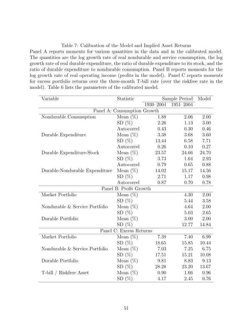
Table 7: Calibration of the Model and Implied Asset ReturnsPanel A reports moments for various quantities in the data and in the calibrated model.The quantities are the log growth rate of real nondurable and service consumption, the loggrowth rate of real durable expenditure, the ratio of durable expenditure to its stock, and theratio of durable expenditure to nondurable consumption. Panel B reports moments for thelog growth rate of real operating income (profits in the model). Panel C reports momentsfor excess portfolio returns over the three-month T-bill rate (over the riskfree rate in themodel). Table 6 lists the parameters of the calibrated model.

Variable Statistic Sample Period Model1930–2004 1951–2004

Panel A: Consumption GrowthNondurable Consumption Mean (%) 1.88 2.06 2.00

SD (%) 2.26 1.13 3.00Autocorrel 0.43 0.30 0.46

Durable Expenditure Mean (%) 3.38 3.68 3.60SD (%) 13.44 6.58 7.71Autocorrel 0.26 0.10 0.27

Durable Expenditure-Stock Mean (%) 23.57 24.66 24.70SD (%) 3.73 1.64 2.93Autocorrel 0.79 0.65 0.88

Durable-Nondurable Expenditure Mean (%) 14.02 15.17 14.56SD (%) 2.71 1.17 0.98Autocorrel 0.87 0.70 0.78

Panel B: Profit GrowthMarket Portfolio Mean (%) 4.30 2.00

SD (%) 5.44 3.58Nondurable & Service Portfolio Mean (%) 4.64 2.00

SD (%) 5.03 2.65Durable Portfolio Mean (%) 3.00 2.00

SD (%) 12.77 14.84Panel C: Excess Returns

Market Portfolio Mean (%) 7.39 7.40 6.99SD (%) 18.65 15.85 10.44

Nondurable & Service Portfolio Mean (%) 7.03 7.25 6.75SD (%) 17.51 15.21 10.08

Durable Portfolio Mean (%) 9.81 8.83 9.13SD (%) 28.28 23.20 13.67

T-bill / Riskfree Asset Mean (%) 0.90 1.66 0.96SD (%) 4.17 2.45 0.76

51

Table 8: Predictability of Excess Returns in the ModelWe use the calibrated model to simulate 10,000 samples, each consisting of 50 annual obser-vations. In Panel A, we run a regression of excess returns (over the riskfree rate) onto thelagged durable expenditure-stock ratio and report the mean and the standard deviation ofthe t-statistic across the simulated samples. In Panel B (Panel C), we repeat the same ex-ercise for a regression of the absolute value of excess returns (profit growth) onto the laggeddurable expenditure-stock ratio. Table 6 lists the parameters of the calibrated model.

Statistic PortfolioMarket Nondurables Durables

Panel A: Excess ReturnsMean of t-stat -0.61 -0.60 -0.71SD of t-stat 1.05 1.05 1.04

Panel B: Absolute Excess ReturnsMean of t-stat -0.35 -0.33 -0.54SD of t-stat 1.08 1.08 1.06

Panel C: Absolute Profit GrowthMean of t-stat 1.13 2.59 -1.27SD of t-stat 1.30 1.74 1.13

Table 9: Consumption Betas in the ModelThe table reports the nondurable and the durable consumption beta in the calibrated model.We compute the betas through a regression of excess returns (over the riskfree rate) ontonondurable consumption growth, durable stock growth, and a constant. Table 6 lists theparameters of the calibrated model.

Statistic PortfolioMarket Nondurables Durables

Nondurable Beta 2.97 2.87 3.87Durable Beta -1.91 -1.84 -2.58

52

Tab

le10

:A

vera

geR

eturn

san

dB

etas

for

the

Fam

a-Fre

nch

and

the

PC

EPor

tfol

ios

Pan

elA

repor

tsav

erag

eex

cess

retu

rns

onth

eth

ree

Fam

a-Fre

nch

fact

ors

and

the

five

indust

rypor

tfol

ios.

For

the

indust

rypor

tfol

ios,

exce

ssre

turn

sar

eov

erth

eth

ree-

mon

thT

-bill.

Pan

elB

repor

tsth

ebet

asan

dth

eal

phas

for

the

Fam

a-Fre

nch

thre

e-fa

ctor

model

.Pan

elC

repor

tsth

ebet

asan

dth

eal

phas

for

the

consu

mpti

on-b

ased

model

,in

whic

hth

efa

ctor

sar

enon

dura

ble

and

dura

ble

consu

mpti

ongr

owth

.A

llre

turn

san

dal

phas

are

repor

ted

inan

nual

ized

per

centa

geunit

s.T

he

sam

ple

per

iod

is19

51:1

–200

4:4. S

tati

stic

Fam

a-Fre

nch

Por

tfol

ios

Indust

ryPor

tfol

ios

Mar

ket

SM

BH

ML

Ser

vic

esN

ondura

ble

sD

ura

ble

sIn

vest

men

tO

ther

Pan

elA

:E

xce

ssR

eturn

sM

ean

(%)

7.67

2.87

3.92

5.66

8.07

8.19

6.43

7.43

Pan

elB

:Fam

a-Fre

nch

Model

Mar

ket

Bet

a1.

000.

000.

000.

870.

911.

131.

111.

06SM

BB

eta

0.00

1.00

0.00

-0.0

7-0

.29

0.15

0.18

0.17

HM

LB

eta

0.00

0.00

1.00

0.10

0.01

0.15

-0.0

70.

02A

lpha

(%)

0.73

0.99

0.03

-0.5

92.

32-0

.51

-1.2

9-0

.31

Pan

elC

:C

onsu

mpti

on-B

ased

Model

Non

dura

ble

Bet

a5.

431.

870.

154.

794.

017.

456.

695.

51D

ura

ble

Bet

a-0

.65

-0.2

50.

75-1

.01

0.16

-1.4

9-1

.26

-0.7

7A

lpha

(%)

0.03

0.36

0.39

0.80

-0.3

10.

31-1

.00

0.17

53

Table 11: Cross-Sectional Test on the Fama-French and the PCE PortfoliosThe table reports estimated factor risk prices for the Fama-French three-factor model andthe consumption-based model. The test assets are the three Fama-French portfolios andthe five industry portfolios. Estimation is by two-step GMM. HAC standard errors are inparentheses. The mean absolute pricing error (MAE) and R2 are based on the first-stageestimate. The p-values for the J-test are in parentheses.

Factor Price Fama-French Consumption-BasedMarket 3.24

(1.14)SMB 1.05

(1.22)HML 2.60

(1.41)Nondurables 22.30

(25.39)Durables 93.11

(38.87)MAE (%) 0.85 0.42R2 0.67 0.92J-test 12.36 8.21

(0.03) (0.22)

54

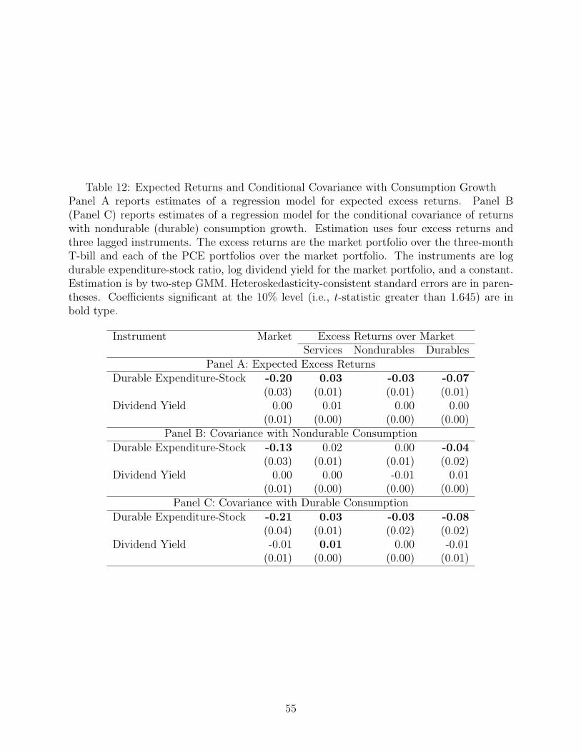
Table 12: Expected Returns and Conditional Covariance with Consumption GrowthPanel A reports estimates of a regression model for expected excess returns. Panel B(Panel C) reports estimates of a regression model for the conditional covariance of returnswith nondurable (durable) consumption growth. Estimation uses four excess returns andthree lagged instruments. The excess returns are the market portfolio over the three-monthT-bill and each of the PCE portfolios over the market portfolio. The instruments are logdurable expenditure-stock ratio, log dividend yield for the market portfolio, and a constant.Estimation is by two-step GMM. Heteroskedasticity-consistent standard errors are in paren-theses. Coefficients significant at the 10% level (i.e., t-statistic greater than 1.645) are inbold type.

Instrument Market Excess Returns over MarketServices Nondurables Durables

Panel A: Expected Excess ReturnsDurable Expenditure-Stock -0.20 0.03 -0.03 -0.07

(0.03) (0.01) (0.01) (0.01)Dividend Yield 0.00 0.01 0.00 0.00

(0.01) (0.00) (0.00) (0.00)Panel B: Covariance with Nondurable Consumption

Durable Expenditure-Stock -0.13 0.02 0.00 -0.04(0.03) (0.01) (0.01) (0.02)

Dividend Yield 0.00 0.00 -0.01 0.01(0.01) (0.00) (0.00) (0.00)

Panel C: Covariance with Durable ConsumptionDurable Expenditure-Stock -0.21 0.03 -0.03 -0.08

(0.04) (0.01) (0.02) (0.02)Dividend Yield -0.01 0.01 0.00 -0.01

(0.01) (0.00) (0.00) (0.01)

55

−30−20−1001020Percent Growth

1951

1961

1971

1981

1991

2001

Yea

r

Sal

es

Dur

able

Exp

endi

ture

(A)

Sal

es o

f Ser

vice

Firm

s

−100102030Percent Growth

1951

1961

1971

1981

1991

2001

Yea

r

(B)

Sal

es o

f Non

dura

ble

Firm

s

−20−1001020Percent Growth

1951

1961

1971

1981

1991

2001

Yea

r

(C)

Sal

es o

f Dur

able

Firm

s

Fig

ure

1:Sal

esG

row

thfo

rth

eP

CE

Por

tfol

ios

The

figu

resh

ows

the

log

annual

grow

thra

teof

sale

sfo

rth

eP

CE

por

tfol

ios.

The

das

hed

line

inea

chpan

elis

the

log

grow

thra

teof

real

dura

ble

expen

dit

ure

.D

ata

onsa

les

are

from

Com

pust

atan

dar

edefl

ated

by

the

CP

I.T

he

sam

ple

per

iod

is19

51–2

004.

56

1950 1955 1960 1965 1970 1975 1980 1985 1990 1995 2000 20055

6

7

8

9

Year

Per

cent

per

Qua

rter

Panel A: Durable Expenditure−Stock Ratio

1950 1955 1960 1965 1970 1975 1980 1985 1990 1995 2000 2005−1

0

1

2

3

4

5

Year

Per

cent

per

Qua

rter

Panel B: Equity Premium

Equity PremiumPremium due to Durables

Figure 2: Time Variation in the Equity PremiumPanel A is a time-series plot of the durable expenditure-stock ratio. Panel B is a time-seriesplot of expected excess returns on the market portfolio over the three-month T-bill rate,implied by the regression model estimated in Table 12. The sample period is 1951:1–2004:3,and the shaded regions are NBER recessions.

57

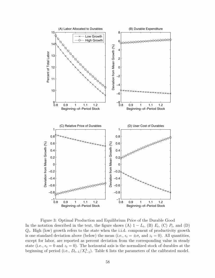
0.8 0.9 1 1.1 1.29

10

11

12

13

14

15(A) Labor Allocated to Durables

Beginning−of−Period Stock

Per

cent

of T

otal

Lab

or

Low GrowthHigh Growth

0.8 0.9 1 1.1 1.2−8

−6

−4

−2

0

2

4

6

8(B) Durable Expenditure

Beginning−of−Period StockD

evia

tion

from

Mea

n G

row

th (

%)

0.8 0.9 1 1.1 1.2−1

−0.8

−0.6

−0.4

−0.2

0

0.2

0.4

0.6

0.8

1(C) Relative Price of Durables

Beginning−of−Period Stock

Dev

iatio

n fr

om M

ean

Gro

wth

(%

)

0.8 0.9 1 1.1 1.2−1

−0.8

−0.6

−0.4

−0.2

0

0.2

0.4

0.6

0.8

1(D) User Cost of Durables

Beginning−of−Period Stock

Dev

iatio

n fr

om M

ean

Gro

wth

(%

)

Figure 3: Optimal Production and Equilibrium Price of the Durable GoodIn the notation described in the text, the figure shows (A) 1 − Lt, (B) Et, (C) Pt, and (D)Qt. High (low) growth refers to the state when the i.i.d. component of productivity growthis one standard deviation above (below) the mean (i.e., εt = ±σε and zt = 0). All quantities,except for labor, are reported as percent deviation from the corresponding value in steadystate (i.e., εt = 0 and zt = 0). The horizontal axis is the normalized stock of durables at thebeginning of period (i.e., Dt−1/X

λt−1). Table 6 lists the parameters of the calibrated model.

58

0.8 0.9 1 1.1 1.2−25

−20

−15

−10

−5

0

5

10

15

20

25(A) Profit of Nondurable Firm

Beginning−of−Period Stock

Dev

iatio

n fr

om M

ean

Gro

wth

(%

)

Low GrowthHigh Growth

0.8 0.9 1 1.1 1.2−25

−20

−15

−10

−5

0

5

10

15

20

25(B) Profit of Durable Firm

Beginning−of−Period StockD

evia

tion

from

Mea

n G

row

th (

%)

0.8 0.9 1 1.1 1.2−3

−2

−1

0

1

2

3(C) Value of Nondurable Firm

Beginning−of−Period Stock

Dev

iatio

n fr

om M

ean

Gro

wth

(%

)

0.8 0.9 1 1.1 1.2−3

−2

−1

0

1

2

3(D) Value of Durable Firm

Beginning−of−Period Stock

Dev

iatio

n fr

om M

ean

Gro

wth

(%

)

Figure 4: Profits and Equilibrium Asset PricesIn the notation described in the text, the figure shows (A) ΠCt, (B) ΠEt, (C) VCt, and (D)VEt. High (low) growth refers to the state when the i.i.d. component of productivity growthis one standard deviation above (below) the mean (i.e., εt = ±σε and zt = 0). All quantitiesare reported as percent deviation from the corresponding value in steady state (i.e., εt = 0and zt = 0). The horizontal axis is the normalized stock of durables at the beginning ofperiod (i.e., Dt−1/X

λt−1). Table 6 lists the parameters of the calibrated model.

59

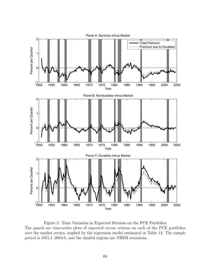
1950 1955 1960 1965 1970 1975 1980 1985 1990 1995 2000 2005−1

0

1

2

Year

Per

cent

per

Qua

rter

Panel A: Services minus Market

Total PremiumPremium due to Durables

1950 1955 1960 1965 1970 1975 1980 1985 1990 1995 2000 2005−1

0

1

2

Year

Per

cent

per

Qua

rter

Panel B: Nondurables minus Market

1950 1955 1960 1965 1970 1975 1980 1985 1990 1995 2000 2005−1

0

1

2

Year

Per

cent

per

Qua

rter

Panel C: Durables minus Market

Figure 5: Time Variation in Expected Returns on the PCE PortfoliosThe panels are time-series plots of expected excess returns on each of the PCE portfoliosover the market return, implied by the regression model estimated in Table 12. The sampleperiod is 1951:1–2004:3, and the shaded regions are NBER recessions.

60