Embed Size (px)
Citation preview
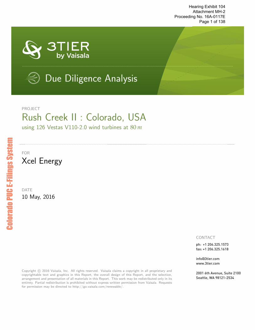
PROJECT
Rush Creek II : Colorado, USAusing 126 Vestas V110-2.0 wind turbines at 80 m
FOR
Xcel Energy
DATE
10 May, 2016
CONTACT
Copyright c© 2016 Vaisala, Inc. All rights reserved. Vaisala claims a copyright in all proprietary andcopyrightable text and graphics in this Report, the overall design of this Report, and the selection,arrangement and presentation of all materials in this Report. This work may be redistributed only in itsentirety. Partial redistribution is prohibited without express written permission from Vaisala. Requestsfor permission may be directed to http://go.vaisala.com/renewable/.
2001 6th Avenue, Suite 2100Seattle, WA 98121-2534
ph: +1 206.325.1573fax: +1 206.325.1618
Due Diligence Analysis
Hearing Exhibit 104 Attachment MH-2
Proceeding No. 16A-0117E Page 1 of 138
Colo
rado
PUC
E-Fil
ings
Syst
em

Disclaimer
This report has been prepared for the use of the client named in the report for the specific purpose identified in the report.Any other party should not rely upon this report for any other purpose. This report is not be used, circulated, quoted orreferred to, in whole or in part, for any other purpose without the prior written consent of Vaisala, Inc. The conclusions,observations and recommendations contained herein attributed to Vaisala, Inc. constitute the opinions of Vaisala, Inc. Fora complete understanding of the conclusions and opinions, this report should be read in its entirety. To the extent thatstatements, information and opinions provided by the client or others have been used in the preparation of this report,Vaisala, Inc. has relied upon the same to be accurate. While we believe the use of such information provided by othersis reasonable for the purposes of this report, no assurances are intended and no representations or warranties are made.Vaisala, Inc. makes no certification and gives no assurances except as explicitly set forth in this report.
Hearing Exhibit 104 Attachment MH-2
Proceeding No. 16A-0117E Page 2 of 138
Rush Creek IIFor Xcel Energy
. . . . . . . . . . . . . . . . . . . . . . . . . . . . . . . . . . . . . . . . . . . . . . . . . . . . . . . . . . . . . . . . . . . . . . . . . . . . . . . . . . . . . . . . . . . . . . . . . . . . . . . . . . . . . . . . . .
Contents
1 Executive Summary 31.1 Wind Speed Maps . . . . . . . . . . . . . . . . . . . . . . . . . . . . . . . . . . . . . . . . . . . . . . . . 4
2 Methodology 52.1 Wind Resource Assessment Steps . . . . . . . . . . . . . . . . . . . . . . . . . . . . . . . . . . . . . . . . 6
3 Observational Data 73.1 Tower M2196 . . . . . . . . . . . . . . . . . . . . . . . . . . . . . . . . . . . . . . . . . . . . . . . . . . 83.2 Tower M2202 . . . . . . . . . . . . . . . . . . . . . . . . . . . . . . . . . . . . . . . . . . . . . . . . . . 103.3 Tower M2311 . . . . . . . . . . . . . . . . . . . . . . . . . . . . . . . . . . . . . . . . . . . . . . . . . . 123.4 Tower M2313 . . . . . . . . . . . . . . . . . . . . . . . . . . . . . . . . . . . . . . . . . . . . . . . . . . 14
4 Long-term Reference 16
5 Gross Generation 175.1 Wind Resource Variability . . . . . . . . . . . . . . . . . . . . . . . . . . . . . . . . . . . . . . . . . . . . 175.2 Gross Generation Variability . . . . . . . . . . . . . . . . . . . . . . . . . . . . . . . . . . . . . . . . . . . 215.3 Power Curves . . . . . . . . . . . . . . . . . . . . . . . . . . . . . . . . . . . . . . . . . . . . . . . . . . 22
6 Loss Factors 236.1 Availability . . . . . . . . . . . . . . . . . . . . . . . . . . . . . . . . . . . . . . . . . . . . . . . . . . . . 236.2 Curtailment . . . . . . . . . . . . . . . . . . . . . . . . . . . . . . . . . . . . . . . . . . . . . . . . . . . 236.3 Wake Deficit . . . . . . . . . . . . . . . . . . . . . . . . . . . . . . . . . . . . . . . . . . . . . . . . . . . 246.4 Electrical Efficiency . . . . . . . . . . . . . . . . . . . . . . . . . . . . . . . . . . . . . . . . . . . . . . . 256.5 Turbine Efficiency . . . . . . . . . . . . . . . . . . . . . . . . . . . . . . . . . . . . . . . . . . . . . . . . 266.6 Environmental . . . . . . . . . . . . . . . . . . . . . . . . . . . . . . . . . . . . . . . . . . . . . . . . . . 266.7 Aggregate Loss Factor . . . . . . . . . . . . . . . . . . . . . . . . . . . . . . . . . . . . . . . . . . . . . . 27
7 Uncertainty Analysis 297.1 Uncertainty Methodology . . . . . . . . . . . . . . . . . . . . . . . . . . . . . . . . . . . . . . . . . . . . 297.2 Uncertainty Framework Results . . . . . . . . . . . . . . . . . . . . . . . . . . . . . . . . . . . . . . . . . 30
8 Probability of Exceedances 328.1 Alternative Project Size . . . . . . . . . . . . . . . . . . . . . . . . . . . . . . . . . . . . . . . . . . . . . 34
9 Conclusion 35
10 Appendix Turbine Means 3610.1 Vestas V110-2.0 wind turbines at 80 m . . . . . . . . . . . . . . . . . . . . . . . . . . . . . . . . . . . . . 36
11 Appendix Gross Long-term Variability 4211.1 Summary . . . . . . . . . . . . . . . . . . . . . . . . . . . . . . . . . . . . . . . . . . . . . . . . . . . . . 4211.2 Power Capacity Maps . . . . . . . . . . . . . . . . . . . . . . . . . . . . . . . . . . . . . . . . . . . . . . 4311.3 Model Simulations By 3TIER . . . . . . . . . . . . . . . . . . . . . . . . . . . . . . . . . . . . . . . . . . 4411.4 Project-average Long-term Wind Resource Assessment . . . . . . . . . . . . . . . . . . . . . . . . . . . . 4611.5 Project-average Long-term Gross Power Capacity Assessment . . . . . . . . . . . . . . . . . . . . . . . . . 5811.6 Long-term Wind Resource Assessment for Tower M2196 at 80 m . . . . . . . . . . . . . . . . . . . . . . . 6811.7 Long-term Wind Resource Assessment for Tower M2202 at 80 m . . . . . . . . . . . . . . . . . . . . . . . 7011.8 Long-term Wind Resource Assessment for Tower M2311 at 80 m . . . . . . . . . . . . . . . . . . . . . . . 7211.9 Long-term Wind Resource Assessment for Tower M2313 at 80 m . . . . . . . . . . . . . . . . . . . . . . . 74
c© 2016 Vaisala, Inc.1
Hearing Exhibit 104 Attachment MH-2
Proceeding No. 16A-0117E Page 3 of 138

Rush Creek IIFor Xcel Energy
. . . . . . . . . . . . . . . . . . . . . . . . . . . . . . . . . . . . . . . . . . . . . . . . . . . . . . . . . . . . . . . . . . . . . . . . . . . . . . . . . . . . . . . . . . . . . . . . . . . . . . . . . . . . . . . . . .
12 Appendix Validation of Model Results 7612.1 Validation of Model Results at Tower M2196 . . . . . . . . . . . . . . . . . . . . . . . . . . . . . . . . . 7612.2 Validation of Model Results at Tower M2202 . . . . . . . . . . . . . . . . . . . . . . . . . . . . . . . . . 9112.3 Validation of Model Results at Tower M2311 . . . . . . . . . . . . . . . . . . . . . . . . . . . . . . . . . 10612.4 Validation of Model Results at Tower M2313 . . . . . . . . . . . . . . . . . . . . . . . . . . . . . . . . . 121
References 136
c© 2016 Vaisala, Inc.2
Hearing Exhibit 104 Attachment MH-2
Proceeding No. 16A-0117E Page 4 of 138
Executive SummaryRush Creek II
For Xcel Energy
. . . . . . . . . . . . . . . . . . . . . . . . . . . . . . . . . . . . . . . . . . . . . . . . . . . . . . . . . . . . . . . . . . . . . . . . . . . . . . . . . . . . . . . . . . . . . . . . . . . . . . . . . . . . . . . . . .
1 EXECUTIVE SUMMARY. . . . . . . . . . . . . . . . . . . . . . . . . . . . . . . . . . . . . . . . . . . . . . . . . . . . . . . . . . . . . . . . . . . . . . . . . . . . . . . . . . . . . . . . . . . . . . . . . . . . . . . . . . . . . . . . . . . . . . . . . . . . . . . . . . . . . . . .
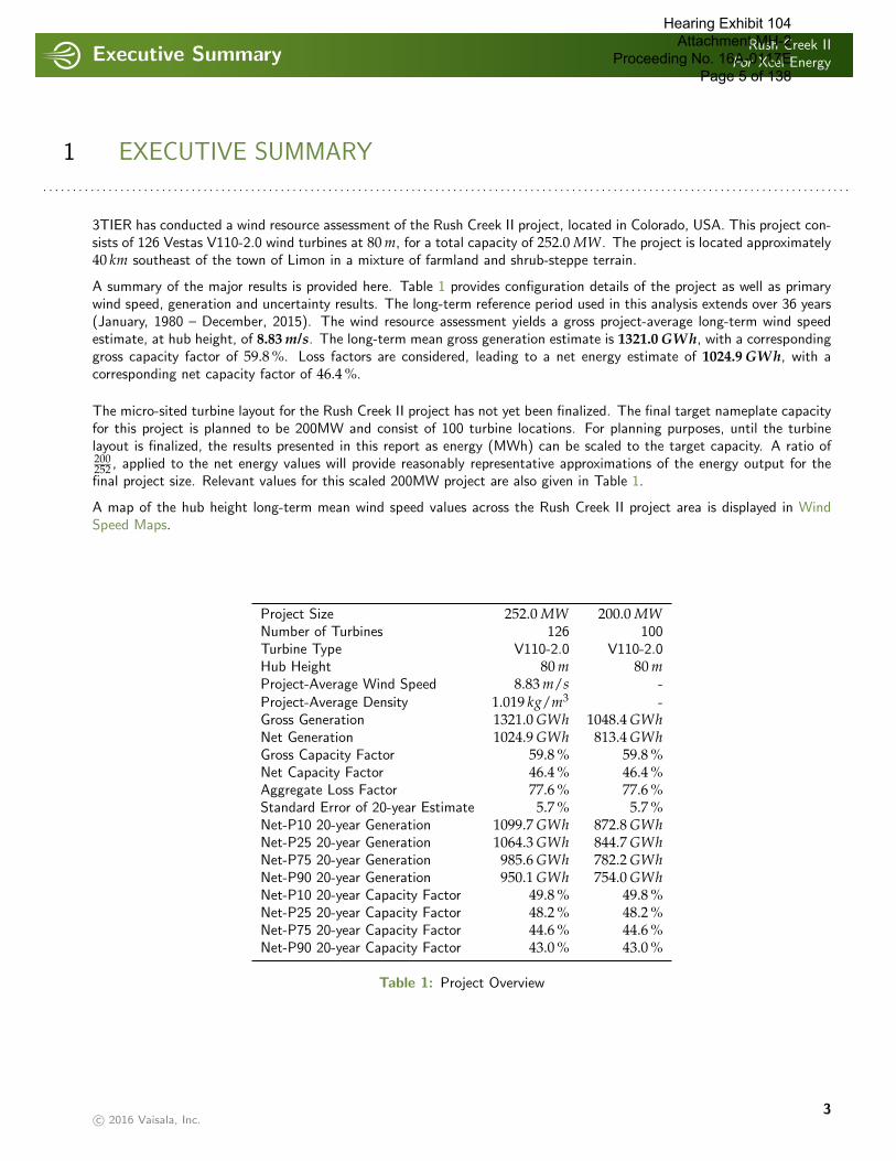
3TIER has conducted a wind resource assessment of the Rush Creek II project, located in Colorado, USA. This project con-sists of 126 Vestas V110-2.0 wind turbines at 80 m, for a total capacity of 252.0 MW. The project is located approximately40 km southeast of the town of Limon in a mixture of farmland and shrub-steppe terrain.
A summary of the major results is provided here. Table 1 provides configuration details of the project as well as primarywind speed, generation and uncertainty results. The long-term reference period used in this analysis extends over 36 years(January, 1980 – December, 2015). The wind resource assessment yields a gross project-average long-term wind speedestimate, at hub height, of 8.83 m/s. The long-term mean gross generation estimate is 1321.0 GWh, with a correspondinggross capacity factor of 59.8 %. Loss factors are considered, leading to a net energy estimate of 1024.9 GWh, with acorresponding net capacity factor of 46.4 %.
The micro-sited turbine layout for the Rush Creek II project has not yet been finalized. The final target nameplate capacityfor this project is planned to be 200MW and consist of 100 turbine locations. For planning purposes, until the turbinelayout is finalized, the results presented in this report as energy (MWh) can be scaled to the target capacity. A ratio of200252 , applied to the net energy values will provide reasonably representative approximations of the energy output for thefinal project size. Relevant values for this scaled 200MW project are also given in Table 1.
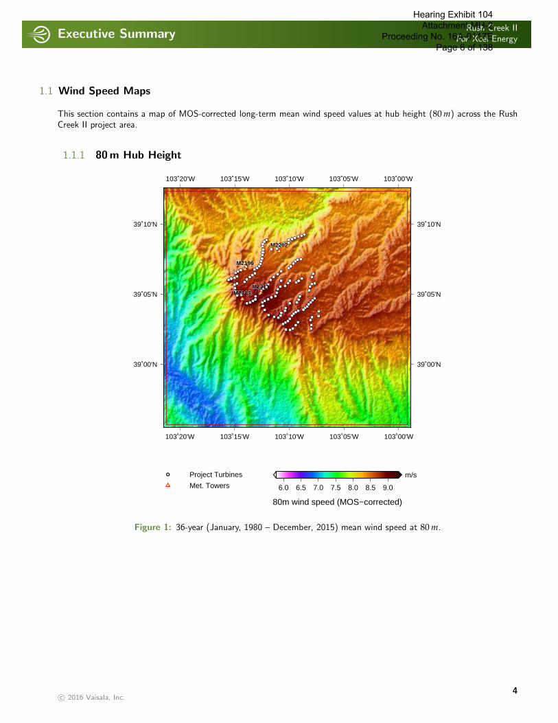
A map of the hub height long-term mean wind speed values across the Rush Creek II project area is displayed in WindSpeed Maps.
Project Size 252.0 MW 200.0 MWNumber of Turbines 126 100Turbine Type V110-2.0 V110-2.0Hub Height 80 m 80 mProject-Average Wind Speed 8.83 m/s -Project-Average Density 1.019 kg/m3 -Gross Generation 1321.0 GWh 1048.4 GWhNet Generation 1024.9 GWh 813.4 GWhGross Capacity Factor 59.8 % 59.8 %Net Capacity Factor 46.4 % 46.4 %Aggregate Loss Factor 77.6 % 77.6 %Standard Error of 20-year Estimate 5.7 % 5.7 %Net-P10 20-year Generation 1099.7 GWh 872.8 GWhNet-P25 20-year Generation 1064.3 GWh 844.7 GWhNet-P75 20-year Generation 985.6 GWh 782.2 GWhNet-P90 20-year Generation 950.1 GWh 754.0 GWhNet-P10 20-year Capacity Factor 49.8 % 49.8 %Net-P25 20-year Capacity Factor 48.2 % 48.2 %Net-P75 20-year Capacity Factor 44.6 % 44.6 %Net-P90 20-year Capacity Factor 43.0 % 43.0 %
Table 1: Project Overview
c© 2016 Vaisala, Inc.3
Hearing Exhibit 104 Attachment MH-2
Proceeding No. 16A-0117E Page 5 of 138
Executive SummaryRush Creek II
For Xcel Energy
. . . . . . . . . . . . . . . . . . . . . . . . . . . . . . . . . . . . . . . . . . . . . . . . . . . . . . . . . . . . . . . . . . . . . . . . . . . . . . . . . . . . . . . . . . . . . . . . . . . . . . . . . . . . . . . . . .
1.1 Wind Speed Maps
This section contains a map of MOS-corrected long-term mean wind speed values at hub height (80 m) across the RushCreek II project area.
1.1.1 80 m Hub Height
103˚20'W
103˚20'W
103˚15'W
103˚15'W
103˚10'W
103˚10'W
103˚05'W
103˚05'W
103˚00'W
103˚00'W
39˚00'N 39˚00'N
39˚05'N 39˚05'N
39˚10'N 39˚10'N
M2196
M2202
M2311M2313
6.0 6.5 7.0 7.5 8.0 8.5 9.0
80m wind speed (MOS−corrected)
m/sProject Turbines
Met. Towers
Figure 1: 36-year (January, 1980 – December, 2015) mean wind speed at 80 m.
c© 2016 Vaisala, Inc.4
Hearing Exhibit 104 Attachment MH-2
Proceeding No. 16A-0117E Page 6 of 138
MethodologyRush Creek II
For Xcel Energy
. . . . . . . . . . . . . . . . . . . . . . . . . . . . . . . . . . . . . . . . . . . . . . . . . . . . . . . . . . . . . . . . . . . . . . . . . . . . . . . . . . . . . . . . . . . . . . . . . . . . . . . . . . . . . . . . . .
2 METHODOLOGY. . . . . . . . . . . . . . . . . . . . . . . . . . . . . . . . . . . . . . . . . . . . . . . . . . . . . . . . . . . . . . . . . . . . . . . . . . . . . . . . . . . . . . . . . . . . . . . . . . . . . . . . . . . . . . . . . . . . . . . . . . . . . . . . . . . . . . . .
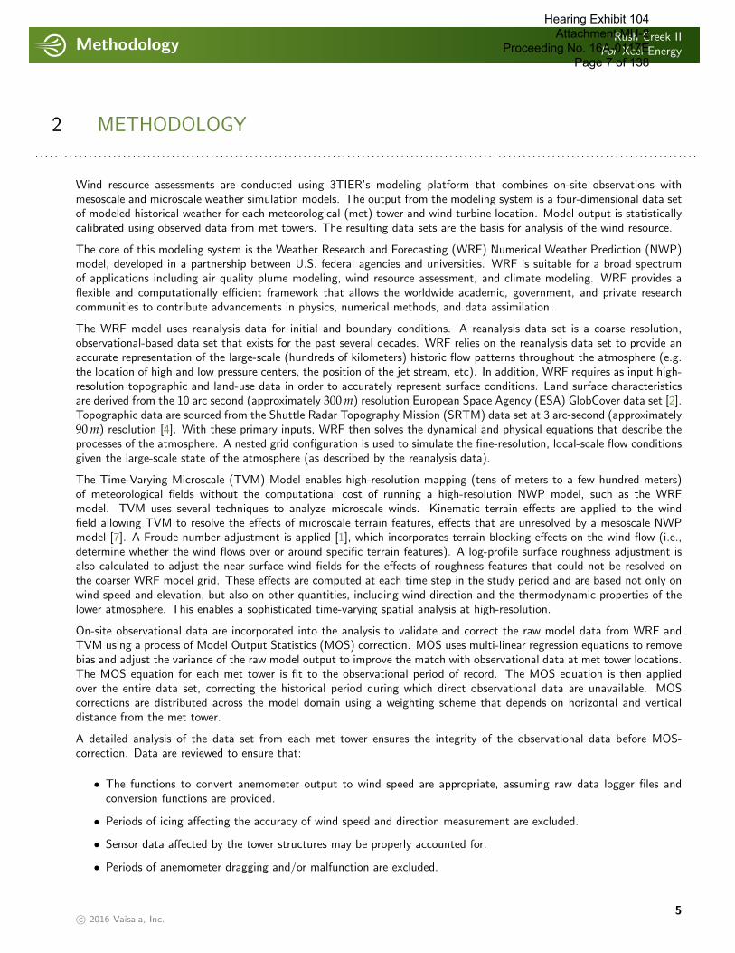
Wind resource assessments are conducted using 3TIER’s modeling platform that combines on-site observations withmesoscale and microscale weather simulation models. The output from the modeling system is a four-dimensional data setof modeled historical weather for each meteorological (met) tower and wind turbine location. Model output is statisticallycalibrated using observed data from met towers. The resulting data sets are the basis for analysis of the wind resource.
The core of this modeling system is the Weather Research and Forecasting (WRF) Numerical Weather Prediction (NWP)model, developed in a partnership between U.S. federal agencies and universities. WRF is suitable for a broad spectrumof applications including air quality plume modeling, wind resource assessment, and climate modeling. WRF provides aflexible and computationally efficient framework that allows the worldwide academic, government, and private researchcommunities to contribute advancements in physics, numerical methods, and data assimilation.
The WRF model uses reanalysis data for initial and boundary conditions. A reanalysis data set is a coarse resolution,observational-based data set that exists for the past several decades. WRF relies on the reanalysis data set to provide anaccurate representation of the large-scale (hundreds of kilometers) historic flow patterns throughout the atmosphere (e.g.the location of high and low pressure centers, the position of the jet stream, etc). In addition, WRF requires as input high-resolution topographic and land-use data in order to accurately represent surface conditions. Land surface characteristicsare derived from the 10 arc second (approximately 300 m) resolution European Space Agency (ESA) GlobCover data set [2].Topographic data are sourced from the Shuttle Radar Topography Mission (SRTM) data set at 3 arc-second (approximately90 m) resolution [4]. With these primary inputs, WRF then solves the dynamical and physical equations that describe theprocesses of the atmosphere. A nested grid configuration is used to simulate the fine-resolution, local-scale flow conditionsgiven the large-scale state of the atmosphere (as described by the reanalysis data).
The Time-Varying Microscale (TVM) Model enables high-resolution mapping (tens of meters to a few hundred meters)of meteorological fields without the computational cost of running a high-resolution NWP model, such as the WRFmodel. TVM uses several techniques to analyze microscale winds. Kinematic terrain effects are applied to the windfield allowing TVM to resolve the effects of microscale terrain features, effects that are unresolved by a mesoscale NWPmodel [7]. A Froude number adjustment is applied [1], which incorporates terrain blocking effects on the wind flow (i.e.,determine whether the wind flows over or around specific terrain features). A log-profile surface roughness adjustment isalso calculated to adjust the near-surface wind fields for the effects of roughness features that could not be resolved onthe coarser WRF model grid. These effects are computed at each time step in the study period and are based not only onwind speed and elevation, but also on other quantities, including wind direction and the thermodynamic properties of thelower atmosphere. This enables a sophisticated time-varying spatial analysis at high-resolution.
On-site observational data are incorporated into the analysis to validate and correct the raw model data from WRF andTVM using a process of Model Output Statistics (MOS) correction. MOS uses multi-linear regression equations to removebias and adjust the variance of the raw model output to improve the match with observational data at met tower locations.The MOS equation for each met tower is fit to the observational period of record. The MOS equation is then appliedover the entire data set, correcting the historical period during which direct observational data are unavailable. MOScorrections are distributed across the model domain using a weighting scheme that depends on horizontal and verticaldistance from the met tower.
A detailed analysis of the data set from each met tower ensures the integrity of the observational data before MOS-correction. Data are reviewed to ensure that:
• The functions to convert anemometer output to wind speed are appropriate, assuming raw data logger files andconversion functions are provided.
• Periods of icing affecting the accuracy of wind speed and direction measurement are excluded.
• Sensor data affected by the tower structures may be properly accounted for.
• Periods of anemometer dragging and/or malfunction are excluded.
c© 2016 Vaisala, Inc.5
Hearing Exhibit 104 Attachment MH-2
Proceeding No. 16A-0117E Page 7 of 138

MethodologyRush Creek II
For Xcel Energy
. . . . . . . . . . . . . . . . . . . . . . . . . . . . . . . . . . . . . . . . . . . . . . . . . . . . . . . . . . . . . . . . . . . . . . . . . . . . . . . . . . . . . . . . . . . . . . . . . . . . . . . . . . . . . . . . . .
During wind project development, met tower sensors are usually placed lower than the hub height of the proposed windturbines. The analysis process must extrapolate the sensor data to hub height using a wind shear coefficient. Wind shearis a meteorological phenomenon in which wind speed values generally increase with height above ground level (AGL); thesurrounding ground cover, trees, and topographic features such as hills and valleys can significantly affect the measuredwind shear. The analysis calculates the shear coefficient from the observed data and then applies the coefficient to highestobserved wind speed data to estimate wind speed values at hub height.
Long-term time series at each proposed turbine location are extracted from the MOS-corrected data set. These hourly timeseries are then combined with the manufacturer’s specified power curve to compute gross capacity factor values. Applyingsite-specific loss factor estimates to the mean P50 gross capacity factor yields the P50 net capacity factor. Uncertainty ofthe measured data and modeling data is then estimated to calculate the final net capacity factors at various probabilitiesof exceedance.
2.1 Wind Resource Assessment Steps
To determine the energy production potential of the proposed Rush Creek II wind project, the following procedure wasimplemented:
1. For the ECMWF ERA-I [3], NCAR/NCEP [5], and MERRA [8] reanalysis data sets, simulate 36 years at 4.5 kmresolution using WRF to understand the long-term temporal variability of weather over the project site.
2. Validate time series data collected from each met tower.
3. Perform correlation analysis between observations and 4.5 km models to determine primary reanalysis data set forNWP modeling.
4. Simulate 1 year at 500 m resolution using WRF to understand the spatial variability of the wind resource at the site.
5. Run TVM to downscale 500 m WRF simulation to 90 m spatial resolution.
6. Perform ensemble analysis to integrate effects of each long term data set including consistency checks to determineusefulness of entire 36 year period for each data set
7. Run MOS to eliminate temporal bias and mitigate spatial bias of WRF/TVM model output. Compute MOScorrections at each met tower. Combine the high-resolution spatial model data with the ensemble adjusted coarserresolution long-term data, creating the final MOS-corrected 90 m resolution long term data set.
8. Calculate the expected (P50) gross capacity factor using modeled long-term time series at each turbine location incombination with the appropriate power curve.
9. Perform numerical wake and turbulence modeling.
10. Apply wake deficit as well as other site-specific loss factor estimates to the gross capacity factor, yielding the expected(P50) net capacity factor.
11. Calculate probability of exceedance levels for the net capacity factor data based on year-to-year wind resourcevariation, measurement uncertainty, and modeling uncertainty.
The following sections provide detail regarding the process outlined above as applied to the Rush Creek II wind project.
c© 2016 Vaisala, Inc.6
Hearing Exhibit 104 Attachment MH-2
Proceeding No. 16A-0117E Page 8 of 138
Observational DataRush Creek II
For Xcel Energy
. . . . . . . . . . . . . . . . . . . . . . . . . . . . . . . . . . . . . . . . . . . . . . . . . . . . . . . . . . . . . . . . . . . . . . . . . . . . . . . . . . . . . . . . . . . . . . . . . . . . . . . . . . . . . . . . . .
3 OBSERVATIONAL DATA. . . . . . . . . . . . . . . . . . . . . . . . . . . . . . . . . . . . . . . . . . . . . . . . . . . . . . . . . . . . . . . . . . . . . . . . . . . . . . . . . . . . . . . . . . . . . . . . . . . . . . . . . . . . . . . . . . . . . . . . . . . . . . . . . . . . . . . .
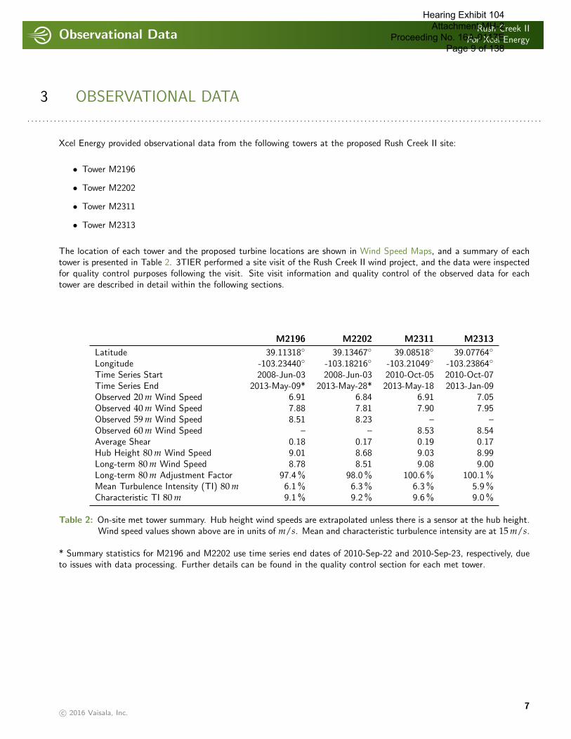
Xcel Energy provided observational data from the following towers at the proposed Rush Creek II site:
• Tower M2196
• Tower M2202
• Tower M2311
• Tower M2313
The location of each tower and the proposed turbine locations are shown in Wind Speed Maps, and a summary of eachtower is presented in Table 2. 3TIER performed a site visit of the Rush Creek II wind project, and the data were inspectedfor quality control purposes following the visit. Site visit information and quality control of the observed data for eachtower are described in detail within the following sections.
M2196 M2202 M2311 M2313
Latitude 39.11318◦ 39.13467◦ 39.08518◦ 39.07764◦
Longitude -103.23440◦ -103.18216◦ -103.21049◦ -103.23864◦
Time Series Start 2008-Jun-03 2008-Jun-03 2010-Oct-05 2010-Oct-07Time Series End 2013-May-09* 2013-May-28* 2013-May-18 2013-Jan-09Observed 20 m Wind Speed 6.91 6.84 6.91 7.05Observed 40 m Wind Speed 7.88 7.81 7.90 7.95Observed 59 m Wind Speed 8.51 8.23 – –Observed 60 m Wind Speed – – 8.53 8.54Average Shear 0.18 0.17 0.19 0.17Hub Height 80 m Wind Speed 9.01 8.68 9.03 8.99Long-term 80 m Wind Speed 8.78 8.51 9.08 9.00Long-term 80 m Adjustment Factor 97.4 % 98.0 % 100.6 % 100.1 %Mean Turbulence Intensity (TI) 80 m 6.1% 6.3 % 6.3 % 5.9 %Characteristic TI 80 m 9.1% 9.2 % 9.6 % 9.0 %
Table 2: On-site met tower summary. Hub height wind speeds are extrapolated unless there is a sensor at the hub height.Wind speed values shown above are in units of m/s. Mean and characteristic turbulence intensity are at 15 m/s.
* Summary statistics for M2196 and M2202 use time series end dates of 2010-Sep-22 and 2010-Sep-23, respectively, dueto issues with data processing. Further details can be found in the quality control section for each met tower.
c© 2016 Vaisala, Inc.7
Hearing Exhibit 104 Attachment MH-2
Proceeding No. 16A-0117E Page 9 of 138
Observational DataRush Creek II
For Xcel Energy
. . . . . . . . . . . . . . . . . . . . . . . . . . . . . . . . . . . . . . . . . . . . . . . . . . . . . . . . . . . . . . . . . . . . . . . . . . . . . . . . . . . . . . . . . . . . . . . . . . . . . . . . . . . . . . . . . .
3.1 Tower M2196
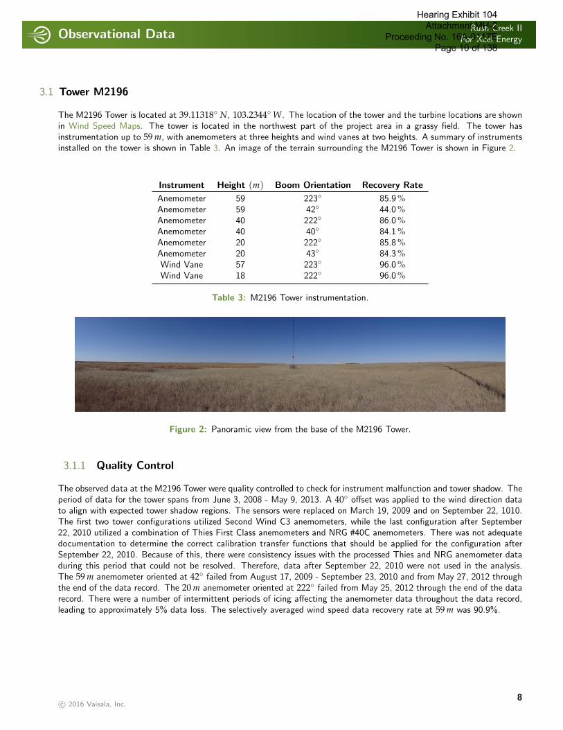
The M2196 Tower is located at 39.11318◦ N, 103.2344◦ W. The location of the tower and the turbine locations are shownin Wind Speed Maps. The tower is located in the northwest part of the project area in a grassy field. The tower hasinstrumentation up to 59 m, with anemometers at three heights and wind vanes at two heights. A summary of instrumentsinstalled on the tower is shown in Table 3. An image of the terrain surrounding the M2196 Tower is shown in Figure 2.
Instrument Height (m) Boom Orientation Recovery Rate
Anemometer 59 223◦ 85.9 %Anemometer 59 42◦ 44.0 %Anemometer 40 222◦ 86.0 %Anemometer 40 40◦ 84.1 %Anemometer 20 222◦ 85.8 %Anemometer 20 43◦ 84.3 %Wind Vane 57 223◦ 96.0 %Wind Vane 18 222◦ 96.0 %
Table 3: M2196 Tower instrumentation.
Figure 2: Panoramic view from the base of the M2196 Tower.
3.1.1 Quality Control
The observed data at the M2196 Tower were quality controlled to check for instrument malfunction and tower shadow. Theperiod of data for the tower spans from June 3, 2008 - May 9, 2013. A 40◦ offset was applied to the wind direction datato align with expected tower shadow regions. The sensors were replaced on March 19, 2009 and on September 22, 1010.The first two tower configurations utilized Second Wind C3 anemometers, while the last configuration after September22, 2010 utilized a combination of Thies First Class anemometers and NRG #40C anemometers. There was not adequatedocumentation to determine the correct calibration transfer functions that should be applied for the configuration afterSeptember 22, 2010. Because of this, there were consistency issues with the processed Thies and NRG anemometer dataduring this period that could not be resolved. Therefore, data after September 22, 2010 were not used in the analysis.The 59 m anemometer oriented at 42◦ failed from August 17, 2009 - September 23, 2010 and from May 27, 2012 throughthe end of the data record. The 20 m anemometer oriented at 222◦ failed from May 25, 2012 through the end of the datarecord. There were a number of intermittent periods of icing affecting the anemometer data throughout the data record,leading to approximately 5% data loss. The selectively averaged wind speed data recovery rate at 59 m was 90.9%.
c© 2016 Vaisala, Inc.8
Hearing Exhibit 104 Attachment MH-2
Proceeding No. 16A-0117E Page 10 of 138
Observational DataRush Creek II
For Xcel Energy
. . . . . . . . . . . . . . . . . . . . . . . . . . . . . . . . . . . . . . . . . . . . . . . . . . . . . . . . . . . . . . . . . . . . . . . . . . . . . . . . . . . . . . . . . . . . . . . . . . . . . . . . . . . . . . . . . .
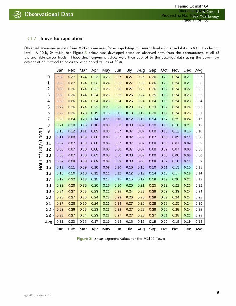
3.1.2 Shear Extrapolation
Observed anemometer data from M2196 were used for extrapolating top sensor level wind speed data to 80 m hub heightlevel. A 12-by-24 table, see Figure 3 below, was developed based on observed data from the anemometers at all ofthe available sensor levels. These shear exponent values were then applied to the observed data using the power lawextrapolation method to calculate wind speed values at 80 m.
Hou
r of
Day
(Lo
cal)
012
34
567
89101112
1314
151617
1819202122
23
Avg
Jan
Jan
Feb
Feb
Mar
Mar
Apr
Apr
May
May
Jun
Jun
Jly
Jly
Aug
Aug
Sep
Sep
Oct
Oct
Nov
Nov
Dec
Dec
Avg
Avg
0.30
0.30
0.30
0.30
0.30
0.29
0.29
0.26
0.21
0.15
0.11
0.09
0.08
0.08
0.09
0.12
0.16
0.19
0.22
0.24
0.25
0.27
0.28
0.29
0.21
0.27
0.27
0.26
0.26
0.26
0.26
0.26
0.24
0.18
0.12
0.08
0.07
0.07
0.07
0.08
0.11
0.16
0.22
0.26
0.27
0.27
0.26
0.26
0.27
0.20
0.24
0.24
0.24
0.24
0.24
0.24
0.23
0.20
0.15
0.11
0.09
0.08
0.08
0.08
0.08
0.09
0.13
0.18
0.23
0.25
0.26
0.25
0.25
0.24
0.18
0.23
0.23
0.23
0.24
0.24
0.22
0.19
0.14
0.10
0.09
0.08
0.08
0.08
0.09
0.09
0.10
0.12
0.15
0.20
0.23
0.24
0.24
0.23
0.23
0.17
0.23
0.24
0.25
0.25
0.23
0.21
0.16
0.11
0.08
0.08
0.08
0.08
0.08
0.08
0.08
0.09
0.11
0.14
0.18
0.22
0.23
0.23
0.23
0.23
0.16
0.27
0.26
0.26
0.25
0.24
0.21
0.15
0.10
0.08
0.07
0.07
0.07
0.08
0.08
0.09
0.10
0.12
0.15
0.20
0.25
0.28
0.29
0.28
0.27
0.18
0.27
0.27
0.27
0.26
0.25
0.23
0.18
0.12
0.08
0.07
0.07
0.07
0.07
0.08
0.08
0.10
0.12
0.15
0.20
0.24
0.26
0.27
0.27
0.27
0.18
0.26
0.25
0.25
0.24
0.24
0.23
0.19
0.13
0.09
0.07
0.07
0.07
0.07
0.07
0.08
0.10
0.12
0.17
0.21
0.25
0.26
0.26
0.26
0.26
0.18
0.26
0.26
0.26
0.25
0.24
0.23
0.20
0.14
0.10
0.08
0.07
0.08
0.08
0.08
0.08
0.10
0.14
0.19
0.25
0.28
0.29
0.28
0.28
0.27
0.19
0.20
0.20
0.19
0.19
0.19
0.19
0.19
0.17
0.13
0.10
0.08
0.08
0.07
0.08
0.09
0.11
0.15
0.19
0.22
0.23
0.23
0.23
0.22
0.21
0.16
0.24
0.24
0.24
0.24
0.24
0.24
0.24
0.22
0.18
0.12
0.09
0.07
0.07
0.08
0.10
0.13
0.17
0.20
0.22
0.23
0.24
0.25
0.25
0.25
0.19
0.21
0.21
0.22
0.23
0.23
0.24
0.25
0.24
0.21
0.16
0.11
0.09
0.08
0.09
0.11
0.15
0.19
0.22
0.23
0.24
0.24
0.24
0.24
0.22
0.19
0.25
0.25
0.25
0.25
0.24
0.23
0.21
0.17
0.13
0.10
0.08
0.08
0.08
0.08
0.09
0.11
0.14
0.18
0.22
0.24
0.25
0.26
0.25
0.25
0.18
Figure 3: Shear exponent values for the M2196 Tower.
c© 2016 Vaisala, Inc.9
Hearing Exhibit 104 Attachment MH-2
Proceeding No. 16A-0117E Page 11 of 138
Observational DataRush Creek II
For Xcel Energy
. . . . . . . . . . . . . . . . . . . . . . . . . . . . . . . . . . . . . . . . . . . . . . . . . . . . . . . . . . . . . . . . . . . . . . . . . . . . . . . . . . . . . . . . . . . . . . . . . . . . . . . . . . . . . . . . . .
3.2 Tower M2202
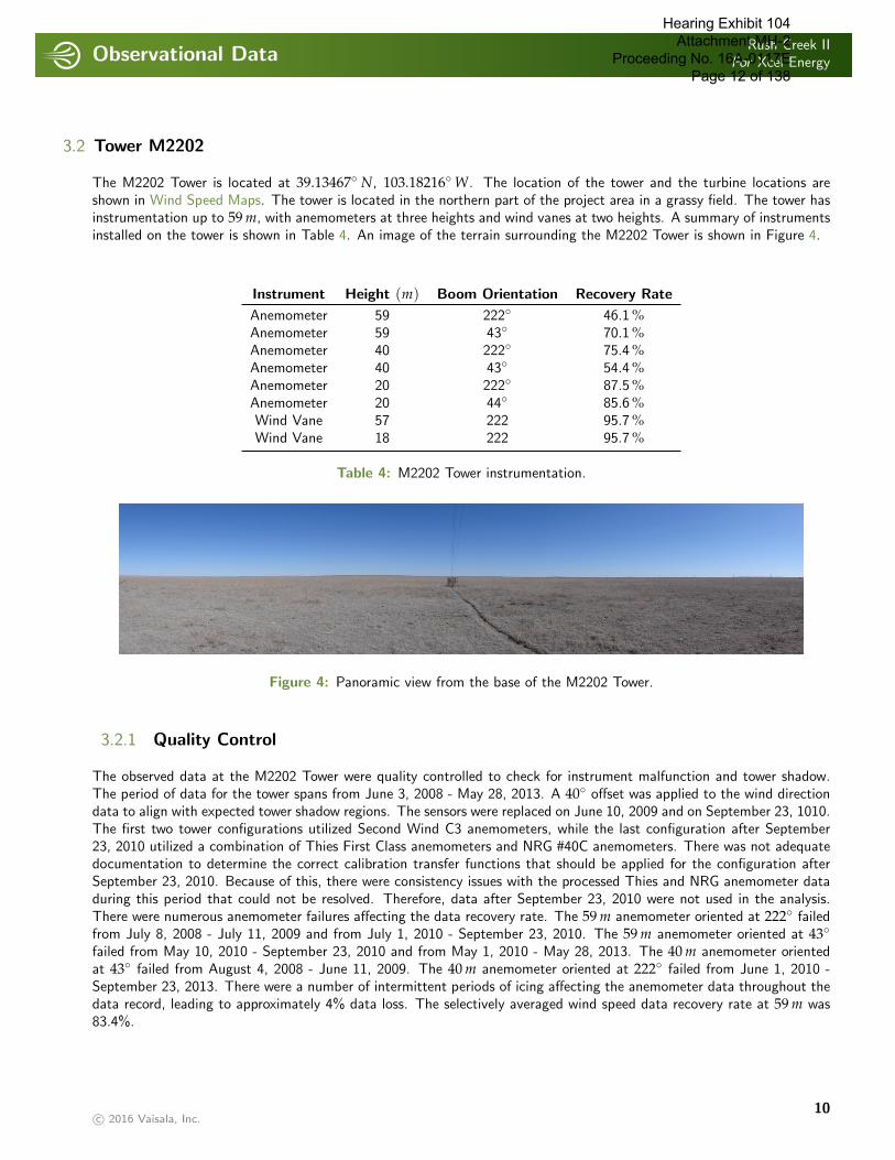
The M2202 Tower is located at 39.13467◦ N, 103.18216◦ W. The location of the tower and the turbine locations areshown in Wind Speed Maps. The tower is located in the northern part of the project area in a grassy field. The tower hasinstrumentation up to 59 m, with anemometers at three heights and wind vanes at two heights. A summary of instrumentsinstalled on the tower is shown in Table 4. An image of the terrain surrounding the M2202 Tower is shown in Figure 4.
Instrument Height (m) Boom Orientation Recovery Rate
Anemometer 59 222◦ 46.1 %Anemometer 59 43◦ 70.1 %Anemometer 40 222◦ 75.4 %Anemometer 40 43◦ 54.4 %Anemometer 20 222◦ 87.5 %Anemometer 20 44◦ 85.6 %Wind Vane 57 222 95.7 %Wind Vane 18 222 95.7 %
Table 4: M2202 Tower instrumentation.
Figure 4: Panoramic view from the base of the M2202 Tower.
3.2.1 Quality Control
The observed data at the M2202 Tower were quality controlled to check for instrument malfunction and tower shadow.The period of data for the tower spans from June 3, 2008 - May 28, 2013. A 40◦ offset was applied to the wind directiondata to align with expected tower shadow regions. The sensors were replaced on June 10, 2009 and on September 23, 1010.The first two tower configurations utilized Second Wind C3 anemometers, while the last configuration after September23, 2010 utilized a combination of Thies First Class anemometers and NRG #40C anemometers. There was not adequatedocumentation to determine the correct calibration transfer functions that should be applied for the configuration afterSeptember 23, 2010. Because of this, there were consistency issues with the processed Thies and NRG anemometer dataduring this period that could not be resolved. Therefore, data after September 23, 2010 were not used in the analysis.There were numerous anemometer failures affecting the data recovery rate. The 59 m anemometer oriented at 222◦ failedfrom July 8, 2008 - July 11, 2009 and from July 1, 2010 - September 23, 2010. The 59 m anemometer oriented at 43◦
failed from May 10, 2010 - September 23, 2010 and from May 1, 2010 - May 28, 2013. The 40 m anemometer orientedat 43◦ failed from August 4, 2008 - June 11, 2009. The 40 m anemometer oriented at 222◦ failed from June 1, 2010 -September 23, 2013. There were a number of intermittent periods of icing affecting the anemometer data throughout thedata record, leading to approximately 4% data loss. The selectively averaged wind speed data recovery rate at 59 m was83.4%.
c© 2016 Vaisala, Inc.10
Hearing Exhibit 104 Attachment MH-2
Proceeding No. 16A-0117E Page 12 of 138
Observational DataRush Creek II
For Xcel Energy
. . . . . . . . . . . . . . . . . . . . . . . . . . . . . . . . . . . . . . . . . . . . . . . . . . . . . . . . . . . . . . . . . . . . . . . . . . . . . . . . . . . . . . . . . . . . . . . . . . . . . . . . . . . . . . . . . .
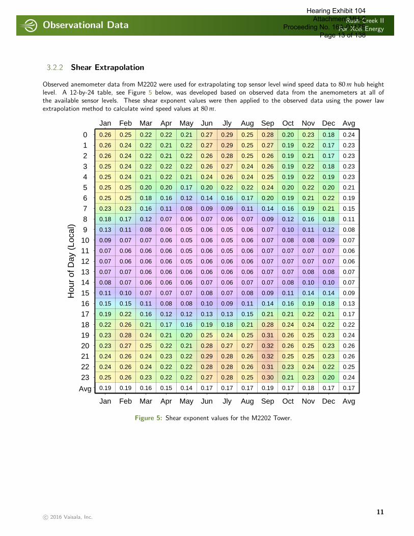
3.2.2 Shear Extrapolation
Observed anemometer data from M2202 were used for extrapolating top sensor level wind speed data to 80 m hub heightlevel. A 12-by-24 table, see Figure 5 below, was developed based on observed data from the anemometers at all ofthe available sensor levels. These shear exponent values were then applied to the observed data using the power lawextrapolation method to calculate wind speed values at 80 m.
Hou
r of
Day
(Lo
cal)
012
34
567
89101112
1314
151617
1819202122
23
Avg
Jan
Jan
Feb
Feb
Mar
Mar
Apr
Apr
May
May
Jun
Jun
Jly
Jly
Aug
Aug
Sep
Sep
Oct
Oct
Nov
Nov
Dec
Dec
Avg
Avg
0.26
0.26
0.26
0.25
0.25
0.25
0.25
0.23
0.18
0.13
0.09
0.07
0.07
0.07
0.08
0.11
0.15
0.19
0.22
0.23
0.23
0.24
0.24
0.25
0.19
0.25
0.24
0.24
0.24
0.24
0.25
0.25
0.23
0.17
0.11
0.07
0.06
0.06
0.07
0.07
0.10
0.15
0.22
0.26
0.28
0.27
0.26
0.26
0.26
0.19
0.22
0.22
0.22
0.22
0.21
0.20
0.18
0.16
0.12
0.08
0.07
0.06
0.06
0.06
0.06
0.07
0.11
0.16
0.21
0.24
0.25
0.24
0.24
0.23
0.16
0.22
0.21
0.21
0.22
0.22
0.20
0.16
0.11
0.07
0.06
0.06
0.06
0.06
0.06
0.06
0.07
0.08
0.12
0.17
0.21
0.22
0.23
0.22
0.22
0.15
0.21
0.22
0.22
0.22
0.21
0.17
0.12
0.08
0.06
0.05
0.05
0.05
0.05
0.06
0.06
0.07
0.08
0.12
0.16
0.20
0.21
0.22
0.22
0.22
0.14
0.27
0.27
0.26
0.26
0.24
0.20
0.14
0.09
0.07
0.06
0.06
0.06
0.06
0.06
0.07
0.08
0.10
0.13
0.19
0.25
0.28
0.29
0.28
0.27
0.17
0.29
0.29
0.28
0.27
0.26
0.22
0.16
0.09
0.06
0.05
0.05
0.05
0.06
0.06
0.06
0.07
0.09
0.13
0.18
0.24
0.27
0.28
0.28
0.28
0.17
0.25
0.25
0.25
0.24
0.24
0.22
0.17
0.11
0.07
0.06
0.06
0.06
0.06
0.06
0.07
0.08
0.11
0.15
0.21
0.25
0.27
0.26
0.26
0.25
0.17
0.28
0.27
0.26
0.26
0.25
0.24
0.20
0.14
0.09
0.07
0.07
0.07
0.07
0.07
0.07
0.09
0.14
0.21
0.28
0.31
0.32
0.32
0.31
0.30
0.19
0.20
0.19
0.19
0.19
0.19
0.20
0.19
0.16
0.12
0.10
0.08
0.07
0.07
0.07
0.08
0.11
0.16
0.21
0.24
0.26
0.26
0.25
0.23
0.21
0.17
0.23
0.22
0.21
0.22
0.22
0.22
0.21
0.19
0.16
0.11
0.08
0.07
0.07
0.08
0.10
0.14
0.19
0.22
0.24
0.25
0.25
0.25
0.24
0.23
0.18
0.18
0.17
0.17
0.18
0.19
0.20
0.22
0.21
0.18
0.12
0.09
0.07
0.07
0.08
0.10
0.14
0.18
0.21
0.22
0.23
0.23
0.23
0.22
0.20
0.17
0.24
0.23
0.23
0.23
0.23
0.21
0.19
0.15
0.11
0.08
0.07
0.06
0.06
0.07
0.07
0.09
0.13
0.17
0.22
0.24
0.26
0.26
0.25
0.24
0.17
Figure 5: Shear exponent values for the M2202 Tower.
c© 2016 Vaisala, Inc.11
Hearing Exhibit 104 Attachment MH-2
Proceeding No. 16A-0117E Page 13 of 138
Observational DataRush Creek II
For Xcel Energy
. . . . . . . . . . . . . . . . . . . . . . . . . . . . . . . . . . . . . . . . . . . . . . . . . . . . . . . . . . . . . . . . . . . . . . . . . . . . . . . . . . . . . . . . . . . . . . . . . . . . . . . . . . . . . . . . . .
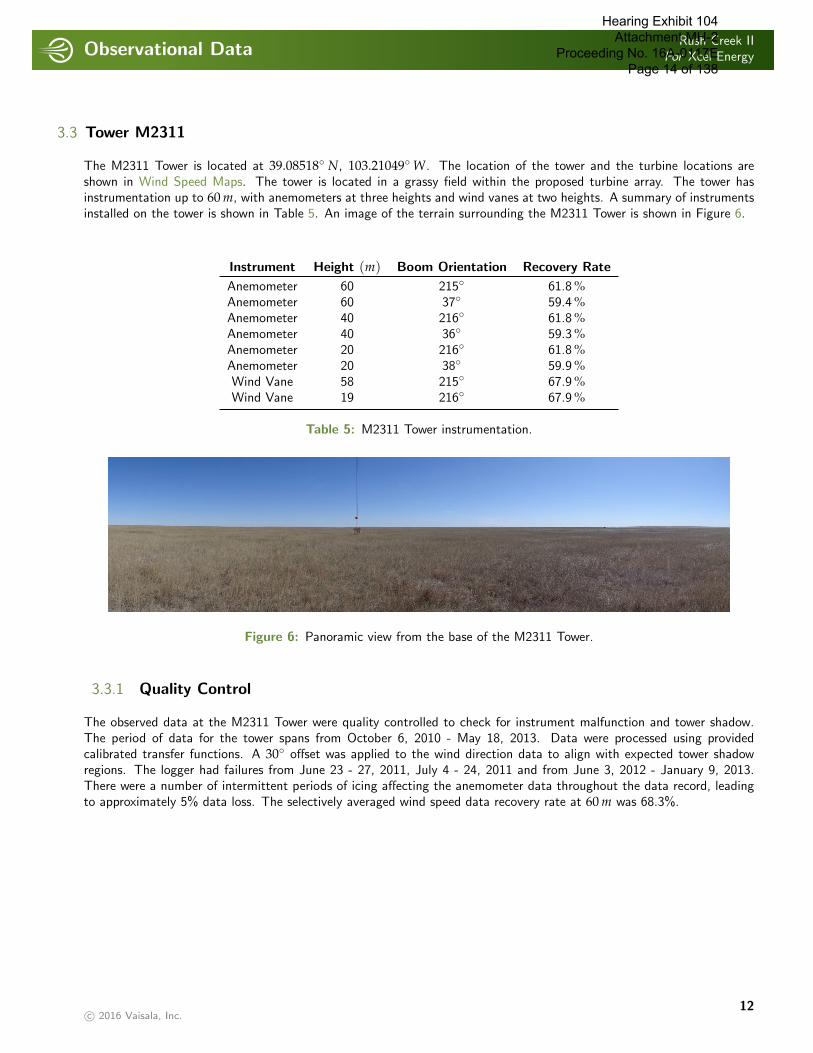
3.3 Tower M2311
The M2311 Tower is located at 39.08518◦ N, 103.21049◦ W. The location of the tower and the turbine locations areshown in Wind Speed Maps. The tower is located in a grassy field within the proposed turbine array. The tower hasinstrumentation up to 60 m, with anemometers at three heights and wind vanes at two heights. A summary of instrumentsinstalled on the tower is shown in Table 5. An image of the terrain surrounding the M2311 Tower is shown in Figure 6.
Instrument Height (m) Boom Orientation Recovery Rate
Anemometer 60 215◦ 61.8 %Anemometer 60 37◦ 59.4 %Anemometer 40 216◦ 61.8 %Anemometer 40 36◦ 59.3 %Anemometer 20 216◦ 61.8 %Anemometer 20 38◦ 59.9 %Wind Vane 58 215◦ 67.9 %Wind Vane 19 216◦ 67.9 %
Table 5: M2311 Tower instrumentation.
Figure 6: Panoramic view from the base of the M2311 Tower.
3.3.1 Quality Control
The observed data at the M2311 Tower were quality controlled to check for instrument malfunction and tower shadow.The period of data for the tower spans from October 6, 2010 - May 18, 2013. Data were processed using providedcalibrated transfer functions. A 30◦ offset was applied to the wind direction data to align with expected tower shadowregions. The logger had failures from June 23 - 27, 2011, July 4 - 24, 2011 and from June 3, 2012 - January 9, 2013.There were a number of intermittent periods of icing affecting the anemometer data throughout the data record, leadingto approximately 5% data loss. The selectively averaged wind speed data recovery rate at 60 m was 68.3%.
c© 2016 Vaisala, Inc.12
Hearing Exhibit 104 Attachment MH-2
Proceeding No. 16A-0117E Page 14 of 138
Observational DataRush Creek II
For Xcel Energy
. . . . . . . . . . . . . . . . . . . . . . . . . . . . . . . . . . . . . . . . . . . . . . . . . . . . . . . . . . . . . . . . . . . . . . . . . . . . . . . . . . . . . . . . . . . . . . . . . . . . . . . . . . . . . . . . . .
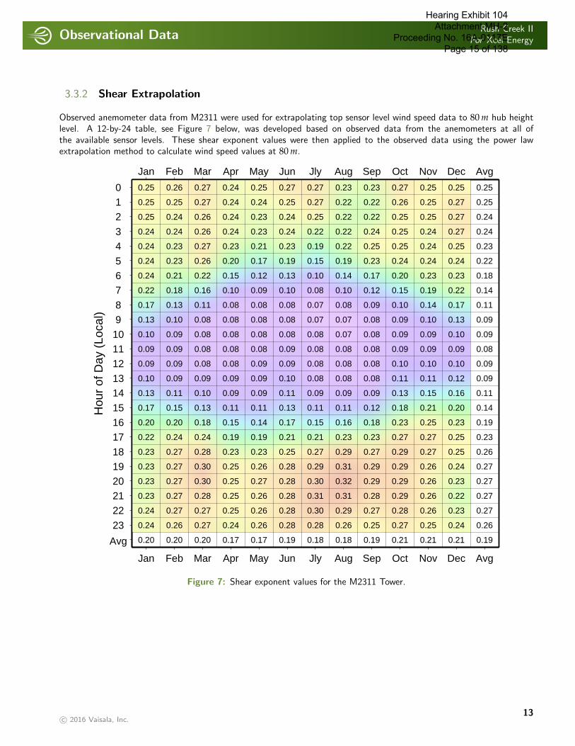
3.3.2 Shear Extrapolation
Observed anemometer data from M2311 were used for extrapolating top sensor level wind speed data to 80 m hub heightlevel. A 12-by-24 table, see Figure 7 below, was developed based on observed data from the anemometers at all ofthe available sensor levels. These shear exponent values were then applied to the observed data using the power lawextrapolation method to calculate wind speed values at 80 m.
Hou
r of
Day
(Lo
cal)
012
34
567
89101112
1314
151617
1819202122
23
Avg
Jan
Jan
Feb
Feb
Mar
Mar
Apr
Apr
May
May
Jun
Jun
Jly
Jly
Aug
Aug
Sep
Sep
Oct
Oct
Nov
Nov
Dec
Dec
Avg
Avg
0.25
0.25
0.25
0.24
0.24
0.24
0.24
0.22
0.17
0.13
0.10
0.09
0.09
0.10
0.13
0.17
0.20
0.22
0.23
0.23
0.23
0.23
0.24
0.24
0.20
0.26
0.25
0.24
0.24
0.23
0.23
0.21
0.18
0.13
0.10
0.09
0.09
0.09
0.09
0.11
0.15
0.20
0.24
0.27
0.27
0.27
0.27
0.27
0.26
0.20
0.27
0.27
0.26
0.26
0.27
0.26
0.22
0.16
0.11
0.08
0.08
0.08
0.08
0.09
0.10
0.13
0.18
0.24
0.28
0.30
0.30
0.28
0.27
0.27
0.20
0.24
0.24
0.24
0.24
0.23
0.20
0.15
0.10
0.08
0.08
0.08
0.08
0.08
0.09
0.09
0.11
0.15
0.19
0.23
0.25
0.25
0.25
0.25
0.24
0.17
0.25
0.24
0.23
0.23
0.21
0.17
0.12
0.09
0.08
0.08
0.08
0.08
0.09
0.09
0.09
0.11
0.14
0.19
0.23
0.26
0.27
0.26
0.26
0.26
0.17
0.27
0.25
0.24
0.24
0.23
0.19
0.13
0.10
0.08
0.08
0.08
0.09
0.09
0.10
0.11
0.13
0.17
0.21
0.25
0.28
0.28
0.28
0.28
0.28
0.19
0.27
0.27
0.25
0.22
0.19
0.15
0.10
0.08
0.07
0.07
0.08
0.08
0.08
0.08
0.09
0.11
0.15
0.21
0.27
0.29
0.30
0.31
0.30
0.28
0.18
0.23
0.22
0.22
0.22
0.22
0.19
0.14
0.10
0.08
0.07
0.07
0.08
0.08
0.08
0.09
0.11
0.16
0.23
0.29
0.31
0.32
0.31
0.29
0.26
0.18
0.23
0.22
0.22
0.24
0.25
0.23
0.17
0.12
0.09
0.08
0.08
0.08
0.08
0.08
0.09
0.12
0.18
0.23
0.27
0.29
0.29
0.28
0.27
0.25
0.19
0.27
0.26
0.25
0.25
0.25
0.24
0.20
0.15
0.10
0.09
0.09
0.09
0.10
0.11
0.13
0.18
0.23
0.27
0.29
0.29
0.29
0.29
0.28
0.27
0.21
0.25
0.25
0.25
0.24
0.24
0.24
0.23
0.19
0.14
0.10
0.09
0.09
0.10
0.11
0.15
0.21
0.25
0.27
0.27
0.26
0.26
0.26
0.26
0.25
0.21
0.25
0.27
0.27
0.27
0.25
0.24
0.23
0.22
0.17
0.13
0.10
0.09
0.10
0.12
0.16
0.20
0.23
0.25
0.25
0.24
0.23
0.22
0.23
0.24
0.21
0.25
0.25
0.24
0.24
0.23
0.22
0.18
0.14
0.11
0.09
0.09
0.08
0.09
0.09
0.11
0.14
0.19
0.23
0.26
0.27
0.27
0.27
0.27
0.26
0.19
Figure 7: Shear exponent values for the M2311 Tower.
c© 2016 Vaisala, Inc.13
Hearing Exhibit 104 Attachment MH-2
Proceeding No. 16A-0117E Page 15 of 138
Observational DataRush Creek II
For Xcel Energy
. . . . . . . . . . . . . . . . . . . . . . . . . . . . . . . . . . . . . . . . . . . . . . . . . . . . . . . . . . . . . . . . . . . . . . . . . . . . . . . . . . . . . . . . . . . . . . . . . . . . . . . . . . . . . . . . . .
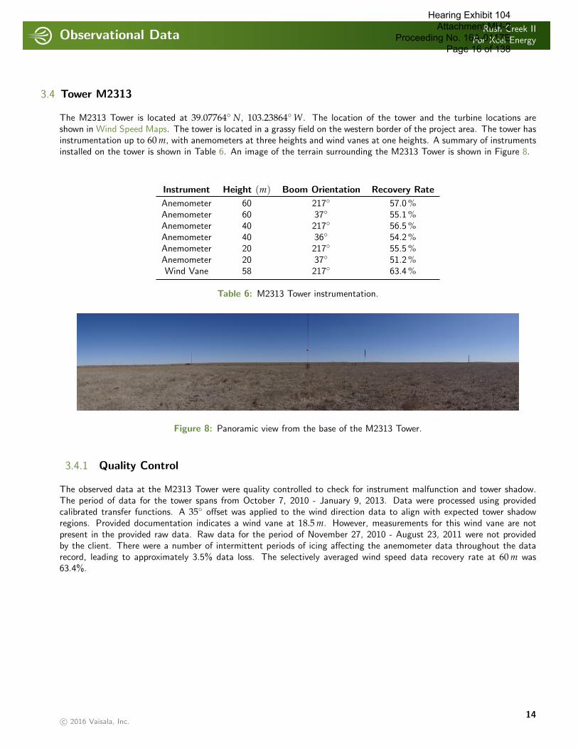
3.4 Tower M2313
The M2313 Tower is located at 39.07764◦ N, 103.23864◦ W. The location of the tower and the turbine locations areshown in Wind Speed Maps. The tower is located in a grassy field on the western border of the project area. The tower hasinstrumentation up to 60 m, with anemometers at three heights and wind vanes at one heights. A summary of instrumentsinstalled on the tower is shown in Table 6. An image of the terrain surrounding the M2313 Tower is shown in Figure 8.
Instrument Height (m) Boom Orientation Recovery Rate
Anemometer 60 217◦ 57.0 %Anemometer 60 37◦ 55.1 %Anemometer 40 217◦ 56.5 %Anemometer 40 36◦ 54.2 %Anemometer 20 217◦ 55.5 %Anemometer 20 37◦ 51.2 %Wind Vane 58 217◦ 63.4 %
Table 6: M2313 Tower instrumentation.
Figure 8: Panoramic view from the base of the M2313 Tower.
3.4.1 Quality Control
The observed data at the M2313 Tower were quality controlled to check for instrument malfunction and tower shadow.The period of data for the tower spans from October 7, 2010 - January 9, 2013. Data were processed using providedcalibrated transfer functions. A 35◦ offset was applied to the wind direction data to align with expected tower shadowregions. Provided documentation indicates a wind vane at 18.5 m. However, measurements for this wind vane are notpresent in the provided raw data. Raw data for the period of November 27, 2010 - August 23, 2011 were not providedby the client. There were a number of intermittent periods of icing affecting the anemometer data throughout the datarecord, leading to approximately 3.5% data loss. The selectively averaged wind speed data recovery rate at 60 m was63.4%.
c© 2016 Vaisala, Inc.14
Hearing Exhibit 104 Attachment MH-2
Proceeding No. 16A-0117E Page 16 of 138
Observational DataRush Creek II
For Xcel Energy
. . . . . . . . . . . . . . . . . . . . . . . . . . . . . . . . . . . . . . . . . . . . . . . . . . . . . . . . . . . . . . . . . . . . . . . . . . . . . . . . . . . . . . . . . . . . . . . . . . . . . . . . . . . . . . . . . .
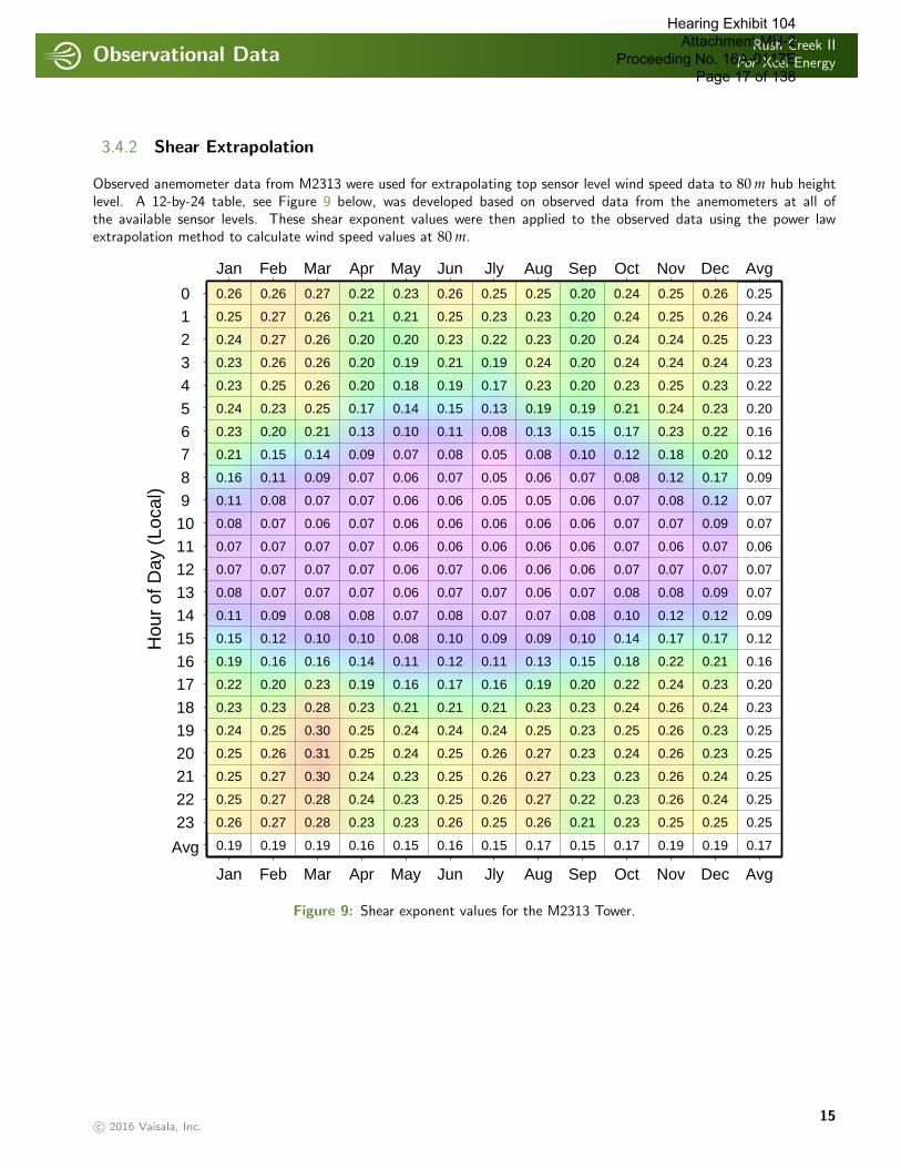
3.4.2 Shear Extrapolation
Observed anemometer data from M2313 were used for extrapolating top sensor level wind speed data to 80 m hub heightlevel. A 12-by-24 table, see Figure 9 below, was developed based on observed data from the anemometers at all ofthe available sensor levels. These shear exponent values were then applied to the observed data using the power lawextrapolation method to calculate wind speed values at 80 m.
Hou
r of
Day
(Lo
cal)
012
34
567
89101112
1314
151617
1819202122
23
Avg
Jan
Jan
Feb
Feb
Mar
Mar
Apr
Apr
May
May
Jun
Jun
Jly
Jly
Aug
Aug
Sep
Sep
Oct
Oct
Nov
Nov
Dec
Dec
Avg
Avg
0.26
0.25
0.24
0.23
0.23
0.24
0.23
0.21
0.16
0.11
0.08
0.07
0.07
0.08
0.11
0.15
0.19
0.22
0.23
0.24
0.25
0.25
0.25
0.26
0.19
0.26
0.27
0.27
0.26
0.25
0.23
0.20
0.15
0.11
0.08
0.07
0.07
0.07
0.07
0.09
0.12
0.16
0.20
0.23
0.25
0.26
0.27
0.27
0.27
0.19
0.27
0.26
0.26
0.26
0.26
0.25
0.21
0.14
0.09
0.07
0.06
0.07
0.07
0.07
0.08
0.10
0.16
0.23
0.28
0.30
0.31
0.30
0.28
0.28
0.19
0.22
0.21
0.20
0.20
0.20
0.17
0.13
0.09
0.07
0.07
0.07
0.07
0.07
0.07
0.08
0.10
0.14
0.19
0.23
0.25
0.25
0.24
0.24
0.23
0.16
0.23
0.21
0.20
0.19
0.18
0.14
0.10
0.07
0.06
0.06
0.06
0.06
0.06
0.06
0.07
0.08
0.11
0.16
0.21
0.24
0.24
0.23
0.23
0.23
0.15
0.26
0.25
0.23
0.21
0.19
0.15
0.11
0.08
0.07
0.06
0.06
0.06
0.07
0.07
0.08
0.10
0.12
0.17
0.21
0.24
0.25
0.25
0.25
0.26
0.16
0.25
0.23
0.22
0.19
0.17
0.13
0.08
0.05
0.05
0.05
0.06
0.06
0.06
0.07
0.07
0.09
0.11
0.16
0.21
0.24
0.26
0.26
0.26
0.25
0.15
0.25
0.23
0.23
0.24
0.23
0.19
0.13
0.08
0.06
0.05
0.06
0.06
0.06
0.06
0.07
0.09
0.13
0.19
0.23
0.25
0.27
0.27
0.27
0.26
0.17
0.20
0.20
0.20
0.20
0.20
0.19
0.15
0.10
0.07
0.06
0.06
0.06
0.06
0.07
0.08
0.10
0.15
0.20
0.23
0.23
0.23
0.23
0.22
0.21
0.15
0.24
0.24
0.24
0.24
0.23
0.21
0.17
0.12
0.08
0.07
0.07
0.07
0.07
0.08
0.10
0.14
0.18
0.22
0.24
0.25
0.24
0.23
0.23
0.23
0.17
0.25
0.25
0.24
0.24
0.25
0.24
0.23
0.18
0.12
0.08
0.07
0.06
0.07
0.08
0.12
0.17
0.22
0.24
0.26
0.26
0.26
0.26
0.26
0.25
0.19
0.26
0.26
0.25
0.24
0.23
0.23
0.22
0.20
0.17
0.12
0.09
0.07
0.07
0.09
0.12
0.17
0.21
0.23
0.24
0.23
0.23
0.24
0.24
0.25
0.19
0.25
0.24
0.23
0.23
0.22
0.20
0.16
0.12
0.09
0.07
0.07
0.06
0.07
0.07
0.09
0.12
0.16
0.20
0.23
0.25
0.25
0.25
0.25
0.25
0.17
Figure 9: Shear exponent values for the M2313 Tower.
c© 2016 Vaisala, Inc.15
Hearing Exhibit 104 Attachment MH-2
Proceeding No. 16A-0117E Page 17 of 138
Long-term ReferenceRush Creek II
For Xcel Energy
. . . . . . . . . . . . . . . . . . . . . . . . . . . . . . . . . . . . . . . . . . . . . . . . . . . . . . . . . . . . . . . . . . . . . . . . . . . . . . . . . . . . . . . . . . . . . . . . . . . . . . . . . . . . . . . . . .
4 LONG-TERM REFERENCE. . . . . . . . . . . . . . . . . . . . . . . . . . . . . . . . . . . . . . . . . . . . . . . . . . . . . . . . . . . . . . . . . . . . . . . . . . . . . . . . . . . . . . . . . . . . . . . . . . . . . . . . . . . . . . . . . . . . . . . . . . . . . . . . . . . . . . . .
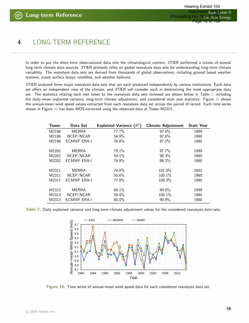
In order to put the short-term observational data into the climatological context, 3TIER performed a review of severallong term climate data sources. 3TIER primarily relies on global reanalysis data sets for understanding long-term climatevariability. The reanalysis data sets are derived from thousands of global observations, including ground based weatherstations, ocean surface buoys, satellites, and weather balloons.
3TIER analyzed three major reanalysis data sets that are each produced independently by various institutions. Each dataset offers an independent view of the climate, and 3TIER will consider each in determining the most appropriate dataset. The statistics relating each met tower to the reanalysis data sets reviewed are shown below in Table 7, includingthe daily-mean explained variance, long-term climate adjustment, and considered start year statistics. Figure 10 showsthe annual-mean wind speed values extracted from each reanalysis data set across the period of record. Each time seriesshown in Figure 10 has been MOS-corrected using the observed data at Tower M2313.
Tower Data Set Explained Variance (R2) Climate Adjustment Start Year
M2196 MERRA 77.7% 97.0% 1999M2196 NCEP/NCAR 54.9% 97.8% 1980M2196 ECMWF ERA-I 78.8% 97.3% 1980
M2202 MERRA 79.1% 97.7% 1999M2202 NCEP/NCAR 59.1% 98.3% 1980M2202 ECMWF ERA-I 78.9% 98.2% 1980
M2311 MERRA 78.0% 101.0% 2002M2311 NCEP/NCAR 55.6% 100.1% 1980M2311 ECMWF ERA-I 77.9% 100.3% 1980
M2313 MERRA 80.1% 99.6% 1999M2313 NCEP/NCAR 59.4% 100.1% 1980M2313 ECMWF ERA-I 80.0% 99.9% 1980
Table 7: Daily explained variance and long-term climate adjustment values for the considered reanalysis data sets.
8.7
8.8
8.9
9.0
9.1
9.2
9.3
9.4
9.5
9.6
9.7
Ann
ual−
mea
n W
ind
Spe
ed (
m/s
)
1980 1984 1988 1992 1996 2000 2004 2008 2012
Year
ERA MERRA NNRP
Figure 10: Time series of annual-mean wind speed data for each considered reanalysis data set.
c© 2016 Vaisala, Inc.16
Hearing Exhibit 104 Attachment MH-2
Proceeding No. 16A-0117E Page 18 of 138
Gross GenerationRush Creek II
For Xcel Energy
. . . . . . . . . . . . . . . . . . . . . . . . . . . . . . . . . . . . . . . . . . . . . . . . . . . . . . . . . . . . . . . . . . . . . . . . . . . . . . . . . . . . . . . . . . . . . . . . . . . . . . . . . . . . . . . . . .
5 GROSS GENERATION. . . . . . . . . . . . . . . . . . . . . . . . . . . . . . . . . . . . . . . . . . . . . . . . . . . . . . . . . . . . . . . . . . . . . . . . . . . . . . . . . . . . . . . . . . . . . . . . . . . . . . . . . . . . . . . . . . . . . . . . . . . . . . . . . . . . . . . .
5.1 Wind Resource Variability
This section provides an analysis of the MOS-corrected model-simulated project-average wind resource at hub height. Togenerate the project-average wind resource time series, MOS-corrected wind resource time series data are extracted ateach turbine location at the appropriate height (80 m) and then averaged across all 126 turbine locations.
Based on the results of 3TIER’s Energy Risk Framework, the last 36 years (January, 1980 – December, 2015) of datahave been utilized for estimating the expected future generation at Rush Creek II. The long-term mean project-averagewind speed at hub height is 8.83 m/s. A map of the 36-year average wind speed values at 80 m is displayed in Figure 1.Gross wind speed values and average density values at each of the 126 turbine locations are provided in Appendix TurbineMeans. The project-average density value at hub height is 1.019 kg/m3.
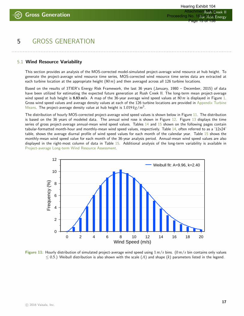
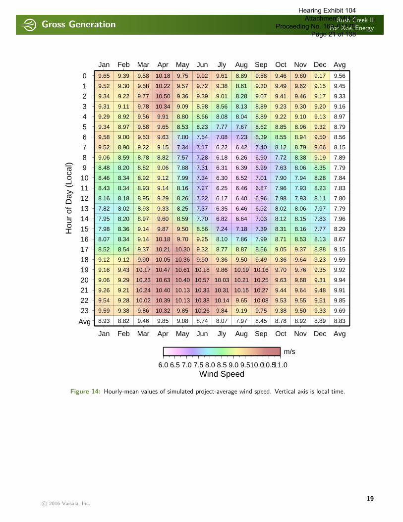
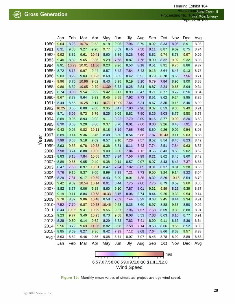
The distribution of hourly MOS-corrected project-average wind speed values is shown below in Figure 11. The distributionis based on the 36 years of modeled data. The annual wind rose is shown in Figure 12. Figure 13 displays the timeseries of gross project-average annual-mean wind speed values. Tables 14 and 15 shown on the following pages containtabular-formatted month-hour and monthly-mean wind speed values, respectively. Table 14, often referred to as a ’12x24’table, shows the average diurnal profile of wind speed values for each month of the calendar year. Table 15 shows themonthly-mean wind speed value for each month of the 36-year analysis period. Annual-mean wind speed values are alsodisplayed in the right-most column of data in Table 15. Additional analysis of the long-term variability is available inProject-average Long-term Wind Resource Assessment.
0 2 4 6 8 10 12 14 16 18 20Wind Speed (m/s)
0
2
4
6
8
10
12
Fre
quen
cy (
%)
Weibull fit: A=9.96, k=2.40
Figure 11: Hourly distribution of simulated project-average wind speed using 1 m/s bins. (0 m/s bin contains only values≤ 0.5.) Weibull distribution is also shown with the scale (A) and shape (k) parameters listed in the legend.
c© 2016 Vaisala, Inc.17
Hearing Exhibit 104 Attachment MH-2
Proceeding No. 16A-0117E Page 19 of 138
Gross GenerationRush Creek II
For Xcel Energy
. . . . . . . . . . . . . . . . . . . . . . . . . . . . . . . . . . . . . . . . . . . . . . . . . . . . . . . . . . . . . . . . . . . . . . . . . . . . . . . . . . . . . . . . . . . . . . . . . . . . . . . . . . . . . . . . . .
S 10 %
EW
N
S 10 %
EW
N
SW
NW
SE
NE
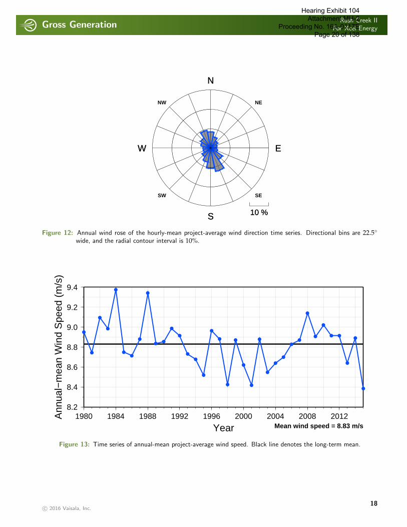
Figure 12: Annual wind rose of the hourly-mean project-average wind direction time series. Directional bins are 22.5◦
wide, and the radial contour interval is 10%.
8.2
8.4
8.6
8.8
9.0
9.2
9.4
Ann
ual−
mea
n W
ind
Spe
ed (
m/s
)
1980 1984 1988 1992 1996 2000 2004 2008 2012
Year Mean wind speed = 8.83 m/s
Figure 13: Time series of annual-mean project-average wind speed. Black line denotes the long-term mean.
c© 2016 Vaisala, Inc.18
Hearing Exhibit 104 Attachment MH-2
Proceeding No. 16A-0117E Page 20 of 138
Gross GenerationRush Creek II
For Xcel Energy
. . . . . . . . . . . . . . . . . . . . . . . . . . . . . . . . . . . . . . . . . . . . . . . . . . . . . . . . . . . . . . . . . . . . . . . . . . . . . . . . . . . . . . . . . . . . . . . . . . . . . . . . . . . . . . . . . .
Hou
r of
Day
(Lo
cal)
012
34
567
89101112
1314
151617
1819202122
23
Avg
Jan
Jan
Feb
Feb
Mar
Mar
Apr
Apr
May
May
Jun
Jun
Jly
Jly
Aug
Aug
Sep
Sep
Oct
Oct
Nov
Nov
Dec
Dec
Avg
Avg
8.52
9.12
9.16
9.06
9.26
9.54
9.59
9.65
9.52
9.34
9.31
9.29
9.34
9.58
9.52
9.06
8.48
8.46
8.43
8.16
7.82
7.95
7.98
8.07
8.93
8.54
9.12
9.43
9.29
9.21
9.28
9.38
9.39
9.30
9.22
9.11
8.92
8.97
9.00
8.90
8.59
8.20
8.34
8.34
8.18
8.02
8.20
8.36
8.34
8.82
9.37
9.90
10.17
10.23
10.24
10.02
9.86
9.58
9.58
9.77
9.78
9.56
9.58
9.53
9.22
8.78
8.82
8.92
8.93
8.95
8.93
8.97
9.14
9.14
9.46
10.21
10.05
10.47
10.63
10.40
10.39
10.32
10.18
10.22
10.50
10.34
9.91
9.65
9.63
9.15
8.82
9.06
9.12
9.14
9.29
9.33
9.60
9.87
10.18
9.85
10.30
10.36
10.61
10.40
10.13
10.13
9.85
9.75
9.57
9.36
9.09
8.80
8.53
7.80
7.34
7.57
7.88
7.99
8.16
8.26
8.25
8.59
9.50
9.70
9.08
9.32
9.90
10.18
10.57
10.33
10.38
10.26
9.92
9.72
9.39
8.98
8.66
8.23
7.54
7.17
7.28
7.31
7.34
7.27
7.22
7.37
7.70
8.56
9.25
8.74
8.77
9.36
9.86
10.03
10.31
10.14
9.84
9.61
9.38
9.01
8.56
8.08
7.77
7.08
6.22
6.18
6.31
6.30
6.25
6.17
6.35
6.82
7.24
8.10
8.07
8.87
9.50
10.19
10.21
10.15
9.65
9.19
8.89
8.61
8.28
8.13
8.04
7.67
7.23
6.42
6.26
6.39
6.52
6.46
6.40
6.46
6.64
7.18
7.86
7.97
8.56
9.49
10.16
10.25
10.27
10.08
9.75
9.58
9.30
9.07
8.89
8.89
8.62
8.39
7.40
6.90
6.99
7.01
6.87
6.96
6.92
7.03
7.39
7.99
8.45
9.05
9.36
9.70
9.63
9.44
9.53
9.38
9.46
9.49
9.41
9.23
9.22
8.85
8.55
8.12
7.72
7.63
7.90
7.96
7.98
8.02
8.12
8.31
8.71
8.78
9.37
9.64
9.76
9.68
9.64
9.55
9.50
9.60
9.62
9.46
9.30
9.10
8.96
8.94
8.79
8.38
8.06
7.94
7.93
7.93
8.06
8.15
8.16
8.53
8.92
8.88
9.23
9.35
9.31
9.48
9.51
9.33
9.17
9.15
9.17
9.20
9.13
9.32
9.50
9.66
9.19
8.35
8.28
8.23
8.11
7.97
7.83
7.77
8.13
8.89
9.15
9.59
9.92
9.94
9.91
9.85
9.69
9.56
9.45
9.33
9.16
8.97
8.79
8.56
8.15
7.89
7.79
7.84
7.83
7.80
7.79
7.96
8.29
8.67
8.83
6.0 6.5 7.0 7.5 8.0 8.5 9.0 9.510.010.511.0Wind Speed
m/s
Figure 14: Hourly-mean values of simulated project-average wind speed. Vertical axis is local time.
c© 2016 Vaisala, Inc.19
Hearing Exhibit 104 Attachment MH-2
Proceeding No. 16A-0117E Page 21 of 138
Gross GenerationRush Creek II
For Xcel Energy
. . . . . . . . . . . . . . . . . . . . . . . . . . . . . . . . . . . . . . . . . . . . . . . . . . . . . . . . . . . . . . . . . . . . . . . . . . . . . . . . . . . . . . . . . . . . . . . . . . . . . . . . . . . . . . . . . .
Yea
r198019811982198319841985198619871988198919901991199219931994199519961997199819992000200120022003200420052006200720082009201020112012201320142015Avg
Jan
Jan
Feb
Feb
Mar
Mar
Apr
Apr
May
May
Jun
Jun
Jly
Jly
Aug
Aug
Sep
Sep
Oct
Oct
Nov
Nov
Dec
Dec
Avg
Avg9.64 8.23 10.76 9.53 9.18 9.05 7.96 8.79 8.92 8.33 8.05 8.91
8.31 9.03 9.27 9.20 9.77 8.59 8.46 7.58 8.11 8.87 9.02 8.75
9.92 8.82 9.61 10.41 8.60 8.89 8.26 7.60 8.52 9.74 8.78 9.97
9.40 8.82 9.65 9.86 9.29 7.68 8.87 7.78 8.90 8.32 9.92 9.32
8.91 10.93 10.01 11.56 9.23 9.26 8.53 8.18 8.51 8.91 9.76 8.86
8.72 8.16 9.97 9.44 8.57 8.42 7.84 8.43 9.16 8.64 8.46 9.13
9.03 8.29 9.03 10.23 8.68 8.55 8.42 8.52 8.79 8.78 8.66 7.56
9.96 8.70 10.96 9.62 8.43 8.95 9.19 8.10 6.79 7.84 8.95 9.00
9.86 8.82 10.65 9.79 11.39 8.73 8.28 8.84 8.87 8.24 9.65 8.94
8.74 8.00 9.54 8.92 9.42 9.17 8.93 8.47 8.71 8.77 8.72 8.56
9.67 8.78 8.64 9.33 9.45 9.55 7.92 7.73 8.51 8.62 9.24 8.85
8.44 8.66 10.25 9.14 10.71 10.09 7.64 8.24 8.67 8.35 9.18 8.46
10.25 8.65 8.80 9.08 9.35 8.47 7.93 7.96 9.07 8.53 9.38 9.49
8.71 8.06 9.73 9.76 8.25 9.05 8.82 7.80 8.26 8.03 8.75 9.50
8.89 9.05 8.93 9.03 9.11 8.22 7.79 8.09 8.16 8.77 9.93 8.20
8.30 8.63 9.20 8.80 9.37 8.70 8.01 7.60 8.00 9.26 8.43 7.91
9.43 9.06 9.82 10.11 9.18 8.19 7.65 7.69 8.60 9.26 9.02 9.54
8.89 9.14 9.36 9.46 8.48 8.80 8.54 6.88 7.87 10.43 9.11 9.63
7.99 8.68 9.18 9.09 8.57 9.10 7.28 7.57 8.52 8.54 8.40 8.23
8.93 9.83 9.78 10.53 9.38 8.81 8.11 7.42 7.74 8.51 7.84 9.63
7.98 8.74 8.88 10.35 9.00 9.00 7.84 7.13 8.56 8.43 8.58 9.02
8.83 8.16 7.84 10.05 8.37 8.34 7.56 7.99 8.21 8.62 8.46 8.60
8.89 9.86 9.05 9.49 9.38 9.14 8.57 9.07 8.97 8.43 8.43 7.37
8.47 7.60 8.97 10.31 8.47 7.94 7.92 8.05 8.31 8.37 8.81 9.28
7.76 9.16 9.37 9.05 8.99 8.38 7.21 7.73 9.50 9.24 9.14 8.22
8.29 7.31 9.17 10.59 8.43 8.90 9.01 7.35 8.32 8.29 10.15 8.54
9.42 9.02 10.54 10.14 8.01 8.44 7.75 7.86 7.76 8.79 8.59 9.60
8.82 8.77 9.06 9.38 8.60 9.10 7.87 8.01 9.31 9.89 8.26 9.39
9.19 9.11 8.84 10.68 10.33 8.16 8.06 8.74 8.44 9.26 9.33 9.54
9.78 8.87 9.86 10.48 8.58 7.69 7.44 8.29 8.63 9.45 8.44 9.34
7.52 7.70 9.87 10.78 10.46 9.23 8.35 8.60 8.97 8.88 9.33 8.50
8.44 10.06 9.41 10.29 9.55 9.37 7.96 7.57 7.58 8.69 9.30 8.88
9.23 9.77 9.40 10.23 8.73 9.68 8.08 8.53 7.88 8.63 8.10 8.77
8.28 9.50 9.14 9.62 8.29 8.73 7.83 7.41 8.90 9.11 8.63 8.36
9.56 8.72 9.63 11.06 8.82 8.98 7.58 7.14 8.53 8.66 9.55 8.52
8.85 8.69 8.27 9.36 8.42 7.39 7.12 8.08 7.64 8.66 8.69 9.57
8.93 8.82 9.46 9.85 9.08 8.74 8.07 7.97 8.45 8.78 8.92 8.89
8.95
8.74
9.09
8.98
9.37
8.75
8.71
8.88
9.34
8.84
8.85
8.99
8.91
8.73
8.68
8.52
8.96
8.88
8.42
8.87
8.62
8.42
8.88
8.55
8.64
8.70
8.83
8.87
9.14
8.91
9.02
8.91
8.91
8.64
8.89
8.38
8.83
6.57.07.58.08.59.09.510.010.511.011.512.0Wind Speed
m/s
Figure 15: Monthly-mean values of simulated project-average wind speed.
c© 2016 Vaisala, Inc.20
Hearing Exhibit 104 Attachment MH-2
Proceeding No. 16A-0117E Page 22 of 138
Gross GenerationRush Creek II
For Xcel Energy
. . . . . . . . . . . . . . . . . . . . . . . . . . . . . . . . . . . . . . . . . . . . . . . . . . . . . . . . . . . . . . . . . . . . . . . . . . . . . . . . . . . . . . . . . . . . . . . . . . . . . . . . . . . . . . . . . .
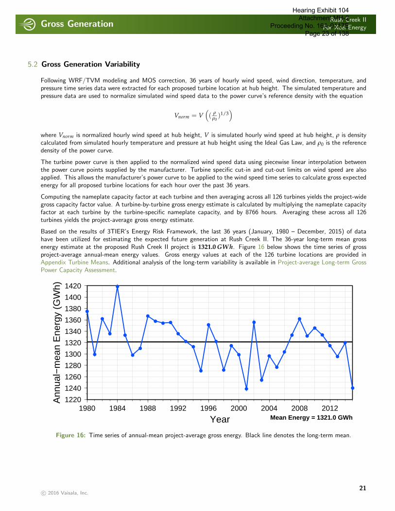
5.2 Gross Generation Variability
Following WRF/TVM modeling and MOS correction, 36 years of hourly wind speed, wind direction, temperature, andpressure time series data were extracted for each proposed turbine location at hub height. The simulated temperature andpressure data are used to normalize simulated wind speed data to the power curve’s reference density with the equation
Vnorm = V(( ρ
ρ0)1/3
)where Vnorm is normalized hourly wind speed at hub height, V is simulated hourly wind speed at hub height, ρ is densitycalculated from simulated hourly temperature and pressure at hub height using the Ideal Gas Law, and ρ0 is the referencedensity of the power curve.
The turbine power curve is then applied to the normalized wind speed data using piecewise linear interpolation betweenthe power curve points supplied by the manufacturer. Turbine specific cut-in and cut-out limits on wind speed are alsoapplied. This allows the manufacturer’s power curve to be applied to the wind speed time series to calculate gross expectedenergy for all proposed turbine locations for each hour over the past 36 years.
Computing the nameplate capacity factor at each turbine and then averaging across all 126 turbines yields the project-widegross capacity factor value. A turbine-by-turbine gross energy estimate is calculated by multiplying the nameplate capacityfactor at each turbine by the turbine-specific nameplate capacity, and by 8766 hours. Averaging these across all 126turbines yields the project-average gross energy estimate.
Based on the results of 3TIER’s Energy Risk Framework, the last 36 years (January, 1980 – December, 2015) of datahave been utilized for estimating the expected future generation at Rush Creek II. The 36-year long-term mean grossenergy estimate at the proposed Rush Creek II project is 1321.0 GWh. Figure 16 below shows the time series of grossproject-average annual-mean energy values. Gross energy values at each of the 126 turbine locations are provided inAppendix Turbine Means. Additional analysis of the long-term variability is available in Project-average Long-term GrossPower Capacity Assessment.
1220
1240
1260
1280
1300
1320
1340
1360
1380
1400
1420
Ann
ual−
mea
n E
nerg
y (G
Wh)
1980 1984 1988 1992 1996 2000 2004 2008 2012
Year Mean Energy = 1321.0 GWh
Figure 16: Time series of annual-mean project-average gross energy. Black line denotes the long-term mean.
c© 2016 Vaisala, Inc.21
Hearing Exhibit 104 Attachment MH-2
Proceeding No. 16A-0117E Page 23 of 138
Gross GenerationRush Creek II
For Xcel Energy
. . . . . . . . . . . . . . . . . . . . . . . . . . . . . . . . . . . . . . . . . . . . . . . . . . . . . . . . . . . . . . . . . . . . . . . . . . . . . . . . . . . . . . . . . . . . . . . . . . . . . . . . . . . . . . . . . .
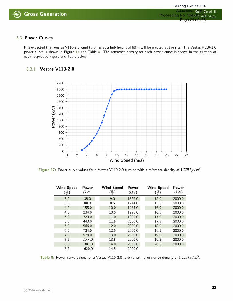
5.3 Power Curves
It is expected that Vestas V110-2.0 wind turbines at a hub height of 80 m will be erected at the site. The Vestas V110-2.0power curve is shown in Figure 17 and Table 8. The reference density for each power curve is shown in the caption ofeach respective Figure and Table below.
5.3.1 Vestas V110-2.0
0
200
400
600
800
1000
1200
1400
1600
1800
2000
2200
Pow
er (
kW)
0 2 4 6 8 10 12 14 16 18 20 22 24
Wind Speed (m/s)
Figure 17: Power curve values for a Vestas V110-2.0 turbine with a reference density of 1.225 kg/m3.
Wind Speed Power Wind Speed Power Wind Speed Power(m
s ) (kW) (ms ) (kW) (m
s ) (kW)
3.0 35.0 9.0 1827.0 15.0 2000.03.5 88.0 9.5 1944.0 15.5 2000.04.0 155.0 10.0 1985.0 16.0 2000.04.5 234.0 10.5 1996.0 16.5 2000.05.0 329.0 11.0 1999.0 17.0 2000.05.5 443.0 11.5 2000.0 17.5 2000.06.0 566.0 12.0 2000.0 18.0 2000.06.5 734.0 12.5 2000.0 18.5 2000.07.0 928.0 13.0 2000.0 19.0 2000.07.5 1144.0 13.5 2000.0 19.5 2000.08.0 1381.0 14.0 2000.0 20.0 2000.08.5 1620.0 14.5 2000.0
Table 8: Power curve values for a Vestas V110-2.0 turbine with a reference density of 1.225 kg/m3.
c© 2016 Vaisala, Inc.22
Hearing Exhibit 104 Attachment MH-2
Proceeding No. 16A-0117E Page 24 of 138
Loss FactorsRush Creek II
For Xcel Energy
. . . . . . . . . . . . . . . . . . . . . . . . . . . . . . . . . . . . . . . . . . . . . . . . . . . . . . . . . . . . . . . . . . . . . . . . . . . . . . . . . . . . . . . . . . . . . . . . . . . . . . . . . . . . . . . . . .
6 LOSS FACTORS. . . . . . . . . . . . . . . . . . . . . . . . . . . . . . . . . . . . . . . . . . . . . . . . . . . . . . . . . . . . . . . . . . . . . . . . . . . . . . . . . . . . . . . . . . . . . . . . . . . . . . . . . . . . . . . . . . . . . . . . . . . . . . . . . . . . . . . .
To convert from expected gross generation to expected net generation, the following loss factor categories are considered:availability, curtailment, wake deficit, electrical efficiency, turbine efficiency, and environmental. Details for each loss factorare discussed below.
6.1 Availability
Availability losses include losses driven by turbine and transmission shutdowns caused by planned and unexpected faults.
6.1.1 Turbine Availability
3TIER has observed that turbine availability at newly constructed wind farms achieve 96.0% or higher availability whenaveraged over an entire calendar year. Therefore, the turbine availability loss factor is estimated to be 96.0%.
6.1.2 Grid Availability
The ability of the electric grid to receive and transmit wind power to load centers varies by year, season and location. Issueswith grid availability are very dynamic and may actually be worsened as wind penetration levels increase. Grid availabilityis expected to be high across the United States. 3TIER has assumed a regional grid availability loss factor of 99.5% forthe Rush Creek II wind energy project.
6.1.3 Balance of Plant Availability
The balance of the plant availability is based on a total of 24 hours of outage time per year per turbine for transformerinspections and maintenance. Therefore, the balance of plant availability loss factor is estimated to be 99.7%.
6.2 Curtailment
Curtailment losses are based on forced wind plant shutdowns resulting from environmental conditions that can adverselyeffect the turbines. These curtailments include wind driven sector management, high wind hysteresis, extreme icing events,and extreme temperatures.
6.2.1 Sector Management
Standard minimum turbine spacing of three rotor diameters perpendicular to the dominant wind direction and five rotordiameters parallel to the dominant wind direction was tested against the layout. Turbine spacing perpendicular to theprevailing wind direction is less than three rotor diameters for a significant number of turbines. Due to the tight spacing,a sector management curtailment loss factor may apply, and the layout should be verified by the turbine manufacturer toensure sector management is properly considered. A quantitative sector management loss calculation may be performed,once details of a sector loss algorithm (if required) are provided by the turbine manufacturer.
c© 2016 Vaisala, Inc.23
Hearing Exhibit 104 Attachment MH-2
Proceeding No. 16A-0117E Page 25 of 138
Loss FactorsRush Creek II
For Xcel Energy
. . . . . . . . . . . . . . . . . . . . . . . . . . . . . . . . . . . . . . . . . . . . . . . . . . . . . . . . . . . . . . . . . . . . . . . . . . . . . . . . . . . . . . . . . . . . . . . . . . . . . . . . . . . . . . . . . .
6.2.2 High Wind Hysteresis
High wind speed hysteresis loss potentially occurs after a turbine has shut down because of a high wind speed cut-outevent. Before the turbine can re-start, the wind speed must slow down to the hysteresis cut-in wind speed. If wind speedvalues reduce to below the cut-out wind speed, but remain above the hysteresis cut-in wind speed, then hysteresis losswill occur. Based on 36 years of modeled hourly wind speed data, cut-out wind speed events are expected to periodicallyoccur. The hysteresis loss factor associated with cut-out events is estimated to be 98.5%.
6.2.3 Extreme Temperature
The Vestas V110-2.0 has an assumed operating temperature between −20◦C and 40◦C without an additional cold weatherpackage. 36 years of MOS-corrected temperature data were analyzed to determine the production losses due to thetemperature constraints. Based on the potential power production during periods with temperatures outside the operatinglimits, and a total wind farm shutdown during these times, the extreme temperature loss factor is estimated to be 99.9%due to extreme temperatures below −20◦C.
6.2.4 Icing Shutdown
Observational data were inspected for significant icing events that may lead an operator to shutdown the wind farm. Theobservational data suggest a curtailment associated with icing events of 99.0%.
6.3 Wake Deficit
3TIER’s wake model is used to determine the expected wake deficit for the turbine layout. The magnitude of the lossesat any given time is a combination of the gross wind field and ambient turbulence intensity across the park, the turbinelayout, and physical characteristics of the installed turbines. 3TIER analyzes wakes using a proprietary time-varying wakemodel that analyzes the wake at every individual time within the simulated record, rather than relying on bulk statisticaldescriptions of the wind field. Wakes for each turbine are computed individually and interact in a physically consistent way,eliminating the need for posterior models to combine wakes from multiple turbines or add in deep-array effects. The singleturbine wake model is based on concepts originally presented by Larsen et al. (1996). [6] 3TIER’s internal research hasshown that the low bias associated with other Larsen-derived wake models [9] is a result of poorly handled wake additionrather than the underlying model. The full system has been calibrated using production numbers from permanentlyinstalled turbines under a wide range of environmental conditions, including a broad span of turbulence intensities andstability regimes. The outputs from the model are wake-induced velocity deficit and turbulence intensity at all turbinelocations, and can include additional reference locations.
6.3.1 Internal Wakes
Internal wakes represent wakes caused by turbines within the project. The effect of wake deficit on energy output for thelayout leads to an internal wake loss factor of 92.7%.
6.3.2 External Wakes
External wakes represent additional wakes caused by turbines from surrounding wind farms. Cedar Point and Limon(Phases 1, 2 and 3) Wind Farms are over 20 km to the northwest of the nearest Rush Creek II project wind turbine. 3TIERconsidered the distances between and positions of project turbines and surrounding turbines within the context of the localwind rose and determined the surrounding wind farms to be inconsequential.
c© 2016 Vaisala, Inc.24
Hearing Exhibit 104 Attachment MH-2
Proceeding No. 16A-0117E Page 26 of 138
Loss FactorsRush Creek II
For Xcel Energy
. . . . . . . . . . . . . . . . . . . . . . . . . . . . . . . . . . . . . . . . . . . . . . . . . . . . . . . . . . . . . . . . . . . . . . . . . . . . . . . . . . . . . . . . . . . . . . . . . . . . . . . . . . . . . . . . . .
6.3.3 Future Wakes
Future wakes represent wakes caused by turbines that will be built in the future, not related to this project. 3TIER utilizedthe Federal Aviation Administration’s (FAA) Wind Turbine Build Out web tool to identify possible future developmentsin the region. 3TIER also directly searched the FAA’s Obstruction Evaluation online database for relevant records ofDetermination of No Hazard to Air Navigation. The closest possible future project filed with the FAA is EDPR’s CrossingTrails project in Kit Carson County, but it is over 20 km to the east and would have no impacts on the Rush Creek II WindFarm. The terrain and expected wind resource immediately north and east, and to some extent to the south, are similarto that of Rush Creek II and could potentially be developed in the future. Such developments would have future wakeimpacts. However, because 3TIER is unaware of any future developments in the immediate area at this time, the futurewakes loss factor is assumed to be 100%.
6.3.4 Total Wakes
The total wake loss factor, including the project (i.e. internal) turbines, is 92.7%. Waked generation values for eachindividual turbine are shown in Appendix Turbine Means.
6.4 Electrical Efficiency
Electrical efficiency considers losses associated with the electrical systems connecting the turbines to the metering point.These systems include the on-site collection system, the substation power transformer, and the transmission line dependingon the meter location. 3TIER assumes the wind farm will be metered on the low side of the substation power transformer.Given this assumption, the electrical system efficiency is expected to be 98.0%.
6.4.1 Collection System Efficiency
The collection system efficiency covers the efficiency of all components from the turbines to the pooling substation,including the medium voltage transformer efficiency that steps up the turbine voltage to the collection system voltage.
6.4.2 Substation Power Transformer Efficiency
The substation power transformer converts the voltage of the collection system to the voltage of the high voltage trans-mission line. This analysis ends at the low side of the substation transformer and does not consider substation powertransformer losses. The client is undertaking a study to determine the full substation loss.
6.4.3 High Voltage Transmission Line Efficiency
Transmission line efficiency is dependent on the cable type, voltage, load, and the distance from the pooling substationto the plant metering point. The client has indicated that the export power will be delivered to a substation that isapproximately 90 miles away which would incur additional high voltage transmission line losses. The client is undertakinga study to determine these added losses. 3TIER has not included an assumption for additional high voltage transmissionline losses in this analysis.
c© 2016 Vaisala, Inc.25
Hearing Exhibit 104 Attachment MH-2
Proceeding No. 16A-0117E Page 27 of 138
Loss FactorsRush Creek II
For Xcel Energy
. . . . . . . . . . . . . . . . . . . . . . . . . . . . . . . . . . . . . . . . . . . . . . . . . . . . . . . . . . . . . . . . . . . . . . . . . . . . . . . . . . . . . . . . . . . . . . . . . . . . . . . . . . . . . . . . . .
6.4.4 Consumptive Power
Consumptive power considers the fact that a wind farm consumes electrical power when generation levels are very low.This is primarily due to power required to keep generators and transformers active and ready for operations. When theplant is operating, consumptive power is inherent to the turbine power curve and electrical efficiency assumptions. Theclient has specified that the wind farm will have a bidirectional meter and has requested that consumptive power of thewind farm be accounted for as an additional loss factor. 3TIER has assumed a loss factor of 99.5% for consumptive power.
6.5 Turbine Efficiency
Turbine efficiency is based on the ability of the turbines to perform at a level relative to the manufacturer’s suggestedperformance rating. This can be affected by many factors, including the manufacturer’s warranted performance level, theturbulence, and inflow angle.
6.5.1 Turbine Performance
3TIER’s experience with operating wind farms suggests a loss factor should be applied for turbine performance. This lossfactor is related to turbines not performing at the manufacturer’s rated power curve. The Vestas V110-2.0 is a relativelynew turbine. Within the United States, there are 5 projects currently under construction with this model and a limitednumber of operating turbines. This turbine model is based on the Vestas V100-2.0, with a longer blade and new gear box.According to a database of installed turbines created by the American Wind Energy Association, there are 2,288 V100-2.0turbines installed in the United States. Based on the lack operational history for the Vestas V110-2.0, 3TIER suggeststhat a turbine performance loss factor of 98.0% be applied to account for the risk that the turbines do not perform exactlyat the manufacturer’s rated power curve.
6.5.2 Turbulence Intensity
Research has linked turbine under performance to stable atmospheric conditions. These conditions are often identifiedby low turbulence intensity. In addition, periods of low or high turbulence intensity can affect the specified power curveby creating a statistical averaging effect. The statistical averaging effect is assessed by comparing the average of theinstantaneous wind speeds using a theoretical zero turbulence power curve against the manufacturer’s power curve atgiven turbulence level. 3TIER analyzes the potential for both of these effects using the measured turbulence intensity andhas calculated a loss factor of 96.9%.
6.5.3 Inflow Angle
Reduced efficiency associated with extreme inflow angles is expected to be negligible; therefore, an inflow angle loss factorof 100.0% is applied.
6.6 Environmental
Potential environmental losses include turbine under-performance caused by turbine blade soiling and degradation, extremeweather conditions such as icing and thunderstorms, and changes to the surrounding environment such as tree growth.
c© 2016 Vaisala, Inc.26
Hearing Exhibit 104 Attachment MH-2
Proceeding No. 16A-0117E Page 28 of 138

Loss FactorsRush Creek II
For Xcel Energy
. . . . . . . . . . . . . . . . . . . . . . . . . . . . . . . . . . . . . . . . . . . . . . . . . . . . . . . . . . . . . . . . . . . . . . . . . . . . . . . . . . . . . . . . . . . . . . . . . . . . . . . . . . . . . . . . . .
6.6.1 Blade Soiling
In locations where the ground is dry and the soil is loose, turbine blades can build up substantial amounts of soil, leadingto a power curve derating. 3TIER has analyzed projects in similar terrain and has calculated a standard loss factor forcultivated farmland and shrub-steppe conditions. A loss factor of 98.5% is applied for blade soiling.
6.6.2 Blade Degradation
Blade degradation, unlike blade soiling, is permanent damage caused to the turbine blades by material in hitting the blades.This can include corrosive material, such as sodium chloride (sea salt), and larger diameter soil and dirt particles. 3TIERhas analyzed projects in similar terrain and has calculated a standard loss factor for cultivated farmland and shrub steppeconditions. A loss factor of 99.5% is applied for blade degradation. While this elevated risk of hail applies to the generalregion, the probability of hail damage at the project or at an individual turbine location is relatively small. No additionalloss factor has been applied for blade degradation due to hail.
6.6.3 Soft Icing
Soft icing occurs when ice builds up on the turbine blades and affects the ability of the turbine to operate optimally. Softicing is often found as shoulder events to hard ice in which loads are exceeded and turbine shutdown occurs. A loss factorof 99.5% is applied for soft icing.
6.6.4 Other Environmental Losses
3TIER has considered the effects from additional environmental losses. Average lightning density for the project is expectedto be moderate relative to the state of Colorado as a whole. Local lightning density is expected to be lower than high risklightning areas in the Midwestern and Southeastern United States. Additional losses such thunderstorms and tree growth,are expected to be negligible.
6.7 Aggregate Loss Factor
Table 9 below shows the individual loss factors for all considered categories and the aggregate loss factor. The product ofall considered losses is 77.6%. The expected gross P50 generation is 1321.0 GWh; therefore, the net P50 generation isthe product of 77.6% and 1321.0 GWh, which equals 1024.9 GWh. Table 10 displays the monthly-mean net values as apercent of the expected annual-mean generation value (GWh).
c© 2016 Vaisala, Inc.27
Hearing Exhibit 104 Attachment MH-2
Proceeding No. 16A-0117E Page 29 of 138
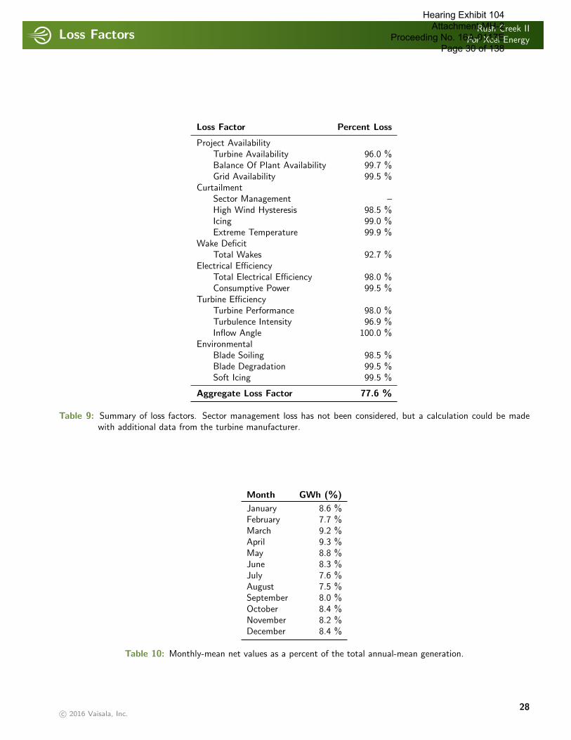
Loss FactorsRush Creek II
For Xcel Energy
. . . . . . . . . . . . . . . . . . . . . . . . . . . . . . . . . . . . . . . . . . . . . . . . . . . . . . . . . . . . . . . . . . . . . . . . . . . . . . . . . . . . . . . . . . . . . . . . . . . . . . . . . . . . . . . . . .
Loss Factor Percent Loss
Project AvailabilityTurbine Availability 96.0 %Balance Of Plant Availability 99.7 %Grid Availability 99.5 %
CurtailmentSector Management –High Wind Hysteresis 98.5 %Icing 99.0 %Extreme Temperature 99.9 %
Wake DeficitTotal Wakes 92.7 %
Electrical EfficiencyTotal Electrical Efficiency 98.0 %Consumptive Power 99.5 %
Turbine EfficiencyTurbine Performance 98.0 %Turbulence Intensity 96.9 %Inflow Angle 100.0 %
EnvironmentalBlade Soiling 98.5 %Blade Degradation 99.5 %Soft Icing 99.5 %
Aggregate Loss Factor 77.6 %
Table 9: Summary of loss factors. Sector management loss has not been considered, but a calculation could be madewith additional data from the turbine manufacturer.
Month GWh (%)
January 8.6 %February 7.7 %March 9.2 %April 9.3 %May 8.8 %June 8.3 %July 7.6 %August 7.5 %September 8.0 %October 8.4 %November 8.2 %December 8.4 %
Table 10: Monthly-mean net values as a percent of the total annual-mean generation.
c© 2016 Vaisala, Inc.28
Hearing Exhibit 104 Attachment MH-2
Proceeding No. 16A-0117E Page 30 of 138

Uncertainty AnalysisRush Creek II
For Xcel Energy
. . . . . . . . . . . . . . . . . . . . . . . . . . . . . . . . . . . . . . . . . . . . . . . . . . . . . . . . . . . . . . . . . . . . . . . . . . . . . . . . . . . . . . . . . . . . . . . . . . . . . . . . . . . . . . . . . .
7 UNCERTAINTY ANALYSIS. . . . . . . . . . . . . . . . . . . . . . . . . . . . . . . . . . . . . . . . . . . . . . . . . . . . . . . . . . . . . . . . . . . . . . . . . . . . . . . . . . . . . . . . . . . . . . . . . . . . . . . . . . . . . . . . . . . . . . . . . . . . . . . . . . . . . . . .
To calculate uncertainty and estimates of probabilities of exceedance, 3TIER has utilized its Energy Risk Framework. Thisframework is based on theoretical propagation of error theory and models hundreds of sources of uncertainty and theirrelationships throughout the modeling process. Each source of uncertainty is treated in a separate model that interactswith the framework through overlying covariance models. The analysis considers the following sources of uncertainty:measurement, vertical extrapolation, MOS correction, climate variability, spatial modeling, and power modeling.
7.1 Uncertainty Methodology
7.1.1 Measurement Uncertainty
Measurement uncertainty captures the uncertainties related to the on-site measured data utilized in the energy assessment.It is a measure of the confidence that the recorded data, which are presumed to represent the truth, actually do representthe truth. Individual components of measurement uncertainty include the following: anemometer uncertainty, benefits ofutilizing redundant sensors, measurement height uncertainty, and the statistical propagation of these uncertainties throughthe wind shear and extrapolation calculations to estimate hub height wind speed values. Uncertainty is separately estimatedfor each measurement sensor, and the sensor uncertainties are aggregated together to represent the total measurementuncertainty at hub height level for each met tower. Measurement uncertainty estimates at each met tower are consideredto be independent when predicting measurement uncertainty at each turbine location.
7.1.2 Vertical Extrapolation Uncertainty
If on-site measurements are not directly recorded at hub height, an uncertainty exists that the true vertical wind speedprofile may differ from the assumed power law profile. A vertical extrapolation uncertainty is required to account for thisuncertainty. Remote sensing and/or hub height measurements can reduce and potentially eliminate this uncertainty.
Vertical extrapolation uncertainty is estimated at each met tower individually and, met tower estimates are combinedassuming partial dependency on the mast and turbine heights when estimating vertical extrapolation uncertainty at theturbine locations. For example, if met towers are located in meteorologically similar environments, risk is increased thatcommon errors are present in the vertical extrapolation process.
7.1.3 MOS Correction Uncertainty
A MOS Correction uncertainty is applied at each met tower that accounts for the probability that the statistical correctionapplied to the long term climate signal will accurately capture the true historic climate variability. The uncertaintyassociated with 3TIER’s MOS correction algorithm decreases as the training period increases. The uncertainty dependson the length of data available at the met tower and the quality of the relationship between the met tower and the longterm data set.
MOS correction uncertainty is estimated at each met tower, and then individual uncertainties are combined to predict theuncertainty at each turbine location assuming partial dependence between each met tower. This dependence is a functionof the concurrency of measurements between the met towers, since the uncertainty of this relationship will depend oncommon errors in the climate signal used as the reference.
c© 2016 Vaisala, Inc.29
Hearing Exhibit 104 Attachment MH-2
Proceeding No. 16A-0117E Page 31 of 138
Uncertainty AnalysisRush Creek II
For Xcel Energy
. . . . . . . . . . . . . . . . . . . . . . . . . . . . . . . . . . . . . . . . . . . . . . . . . . . . . . . . . . . . . . . . . . . . . . . . . . . . . . . . . . . . . . . . . . . . . . . . . . . . . . . . . . . . . . . . . .
7.1.4 Climate Variability Uncertainty
Climate variability uncertainty is comprised of the following individual component uncertainties: historic climate, futureclimate, climate change, and climate signal consistency. Historic and future climate uncertainties represent the uncertaintyassociated with the natural variability of the climate and whether the climate reference period or future prediction periodwill capture the true climate. These uncertainties are a function of the inter-annual variability and auto-correlation ofthe climate signal. Climate change and climate signal consistency uncertainties represent the probability of error of thefuture prediction because the climate of the future may not be accurately represented by the climate of the past. Theseuncertainties are higher if the past few years show potential trends that may point towards a changing pattern.
Climate variability uncertainty is considered common across all met towers and is modeled with complete dependence inthe uncertainty framework.
7.1.5 Spatial Modeling Uncertainty
Spatial modeling uncertainty is estimated by calibrating a spatial model for each met tower that applies the MOS correctionderived at that met tower to all the turbine locations. The individual spatial models are combined at each turbine locationusing weights that are a function of the total uncertainty at each met tower considering dependence and independence ofeach component uncertainty. Spatial uncertainties are a function of the geographic covariance between each met towerand turbine location. 3TIER applies two spatial modeling uncertainties: micro spatial uncertainty and macro spatialuncertainty. Micro spatial uncertainty represents the uncertainty associated with the grid resolution of the spatial modeland whether the model is capturing micro scale effects. Macro spatial uncertainty represents the risk that a spatial modelcalibration at the location of a met tower is applicable at distances away from that met tower.
This complex uncertainty is a function of all the prior uncertainties and relative proximity and complexity of each geospatialrelationship. The dependence on prior uncertainties is driven by the weighting scheme of each met tower, which hasuncertainty dependence. Spatial covariance is also considered when aggregating each individual turbine uncertainty into aproject average uncertainty.
7.1.6 Power Modeling Uncertainty
Power modeling uncertainty considers each step in converting wind speed estimates into energy estimates. In this step,wind speed uncertainties are expanded by the wind speed to energy relationship and then the following is considered:representativeness of the modeled frequency distribution when applying the specified power curve, wakes, availabilities,electrical losses, and all other losses considered in the loss evaluation process. Power modeling uncertainties are consideredto be dependent between each turbine location.
7.2 Uncertainty Framework Results
All uncertainty categories for the Rush Creek II project fall within acceptable ranges for a quality pre-construction duediligence analysis. The project benefits from multiple met towers with redundant anemometry all collecting over a year ofdata. Although the vertical extrapolation uncertainty is relatively low, the project could benefit by collecting wind speedmeasurements at or near hub height to further reduce the vertical extrapolation uncertainty. This can be achieved byinstalling additional met towers with hub height measurements, or by utilizing a wind profiler device such as a Triton SODAR(Sonic Detection and Ranging) or LIDAR (Light Detection and Ranging). 3TIER can provide further recommendationsregarding wind profiler options at the clients request.
c© 2016 Vaisala, Inc.30
Hearing Exhibit 104 Attachment MH-2
Proceeding No. 16A-0117E Page 32 of 138
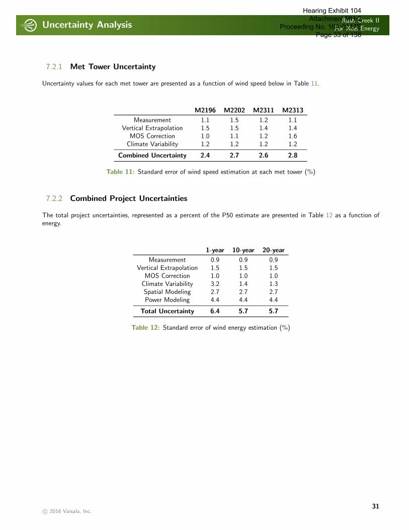
Uncertainty AnalysisRush Creek II
For Xcel Energy
. . . . . . . . . . . . . . . . . . . . . . . . . . . . . . . . . . . . . . . . . . . . . . . . . . . . . . . . . . . . . . . . . . . . . . . . . . . . . . . . . . . . . . . . . . . . . . . . . . . . . . . . . . . . . . . . . .
7.2.1 Met Tower Uncertainty
Uncertainty values for each met tower are presented as a function of wind speed below in Table 11.
M2196 M2202 M2311 M2313
Measurement 1.1 1.5 1.2 1.1Vertical Extrapolation 1.5 1.5 1.4 1.4
MOS Correction 1.0 1.1 1.2 1.6Climate Variability 1.2 1.2 1.2 1.2
Combined Uncertainty 2.4 2.7 2.6 2.8
Table 11: Standard error of wind speed estimation at each met tower (%)
7.2.2 Combined Project Uncertainties
The total project uncertainties, represented as a percent of the P50 estimate are presented in Table 12 as a function ofenergy.
1-year 10-year 20-year
Measurement 0.9 0.9 0.9Vertical Extrapolation 1.5 1.5 1.5
MOS Correction 1.0 1.0 1.0Climate Variability 3.2 1.4 1.3Spatial Modeling 2.7 2.7 2.7Power Modeling 4.4 4.4 4.4
Total Uncertainty 6.4 5.7 5.7
Table 12: Standard error of wind energy estimation (%)
c© 2016 Vaisala, Inc.31
Hearing Exhibit 104 Attachment MH-2
Proceeding No. 16A-0117E Page 33 of 138
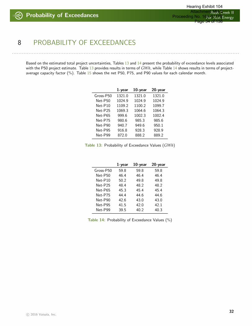
Probability of ExceedancesRush Creek II
For Xcel Energy
. . . . . . . . . . . . . . . . . . . . . . . . . . . . . . . . . . . . . . . . . . . . . . . . . . . . . . . . . . . . . . . . . . . . . . . . . . . . . . . . . . . . . . . . . . . . . . . . . . . . . . . . . . . . . . . . . .
8 PROBABILITY OF EXCEEDANCES. . . . . . . . . . . . . . . . . . . . . . . . . . . . . . . . . . . . . . . . . . . . . . . . . . . . . . . . . . . . . . . . . . . . . . . . . . . . . . . . . . . . . . . . . . . . . . . . . . . . . . . . . . . . . . . . . . . . . . . . . . . . . . . . . . . . . . . .
Based on the estimated total project uncertainties, Tables 13 and 14 present the probability of exceedance levels associatedwith the P50 project estimate. Table 13 provides results in terms of GWh, while Table 14 shows results in terms of project-average capacity factor (%). Table 15 shows the net P50, P75, and P90 values for each calendar month.
1-year 10-year 20-year
Gross-P50 1321.0 1321.0 1321.0Net-P50 1024.9 1024.9 1024.9Net-P10 1109.2 1100.2 1099.7Net-P25 1069.3 1064.6 1064.3Net-P65 999.6 1002.3 1002.4Net-P75 980.6 985.3 985.6Net-P90 940.7 949.6 950.1Net-P95 916.8 928.3 928.9Net-P99 872.0 888.2 889.2
Table 13: Probability of Exceedance Values (GWh)
1-year 10-year 20-year
Gross-P50 59.8 59.8 59.8Net-P50 46.4 46.4 46.4Net-P10 50.2 49.8 49.8Net-P25 48.4 48.2 48.2Net-P65 45.3 45.4 45.4Net-P75 44.4 44.6 44.6Net-P90 42.6 43.0 43.0Net-P95 41.5 42.0 42.1Net-P99 39.5 40.2 40.3
Table 14: Probability of Exceedance Values (%)
c© 2016 Vaisala, Inc.32
Hearing Exhibit 104 Attachment MH-2
Proceeding No. 16A-0117E Page 34 of 138
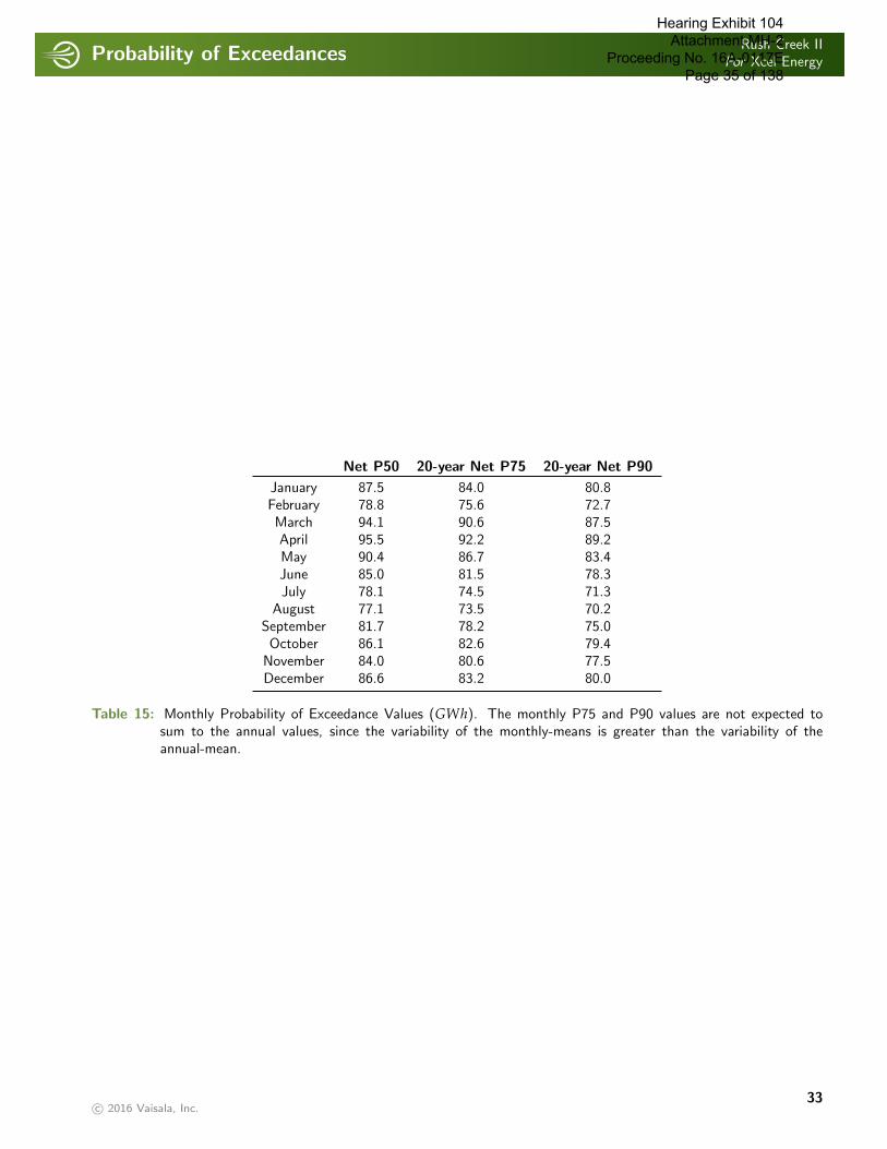
Probability of ExceedancesRush Creek II
For Xcel Energy
. . . . . . . . . . . . . . . . . . . . . . . . . . . . . . . . . . . . . . . . . . . . . . . . . . . . . . . . . . . . . . . . . . . . . . . . . . . . . . . . . . . . . . . . . . . . . . . . . . . . . . . . . . . . . . . . . .
Net P50 20-year Net P75 20-year Net P90
January 87.5 84.0 80.8February 78.8 75.6 72.7March 94.1 90.6 87.5April 95.5 92.2 89.2May 90.4 86.7 83.4June 85.0 81.5 78.3July 78.1 74.5 71.3
August 77.1 73.5 70.2September 81.7 78.2 75.0October 86.1 82.6 79.4
November 84.0 80.6 77.5December 86.6 83.2 80.0
Table 15: Monthly Probability of Exceedance Values (GWh). The monthly P75 and P90 values are not expected tosum to the annual values, since the variability of the monthly-means is greater than the variability of theannual-mean.
c© 2016 Vaisala, Inc.33
Hearing Exhibit 104 Attachment MH-2
Proceeding No. 16A-0117E Page 35 of 138

Probability of ExceedancesRush Creek II
For Xcel Energy
. . . . . . . . . . . . . . . . . . . . . . . . . . . . . . . . . . . . . . . . . . . . . . . . . . . . . . . . . . . . . . . . . . . . . . . . . . . . . . . . . . . . . . . . . . . . . . . . . . . . . . . . . . . . . . . . . .
8.1 Alternative Project Size
The micro-sited turbine layout for the Rush Creek II project has not yet been finalized. The final target nameplate capacityfor this project is planned to be 200MW and consist of 100 turbine locations. For planning purposes, until the turbinelayout is finalized, the results presented in this report as energy (MWh) can be scaled to the target capacity. A ratio of200252 , applied to the net energy values will provide reasonably representative approximations of the energy output for thefinal project size. Table 16 provides the results of this reduced size project in terms of GWh. The project average capacityfactor (%) for this scaled down project remains unchanged.
1-year 10-year 20-year
Gross-P50 1048.4 1048.4 1048.4Net-P50 813.4 813.4 813.4Net-P10 880.3 873.2 872.8Net-P25 848.7 844.9 844.7Net-P65 793.3 795.5 795.6Net-P75 778.3 782.0 782.2Net-P90 746.6 753.7 754.0Net-P95 727.6 736.7 737.2Net-P99 692.1 704.9 705.7
Table 16: Probability of Exceedance Values (GWh)
c© 2016 Vaisala, Inc.34
Hearing Exhibit 104 Attachment MH-2
Proceeding No. 16A-0117E Page 36 of 138
ConclusionRush Creek II
For Xcel Energy
. . . . . . . . . . . . . . . . . . . . . . . . . . . . . . . . . . . . . . . . . . . . . . . . . . . . . . . . . . . . . . . . . . . . . . . . . . . . . . . . . . . . . . . . . . . . . . . . . . . . . . . . . . . . . . . . . .
9 CONCLUSION. . . . . . . . . . . . . . . . . . . . . . . . . . . . . . . . . . . . . . . . . . . . . . . . . . . . . . . . . . . . . . . . . . . . . . . . . . . . . . . . . . . . . . . . . . . . . . . . . . . . . . . . . . . . . . . . . . . . . . . . . . . . . . . . . . . . . . . .
3TIER has conducted a wind resource assessment of the Rush Creek II project. The assessment is based on a wind turbinelayout consisting of 126 Vestas V110-2.0 wind turbines at 80 m. The wind resource assessment yields a gross energy valueof 1321.0 GWh. Loss factors were considered, leading to a net energy estimate of 1024.9 GWh. Turbine-wise values ofgross energy, wake loss, and net energy are available in Appendix Turbine Means. Following the uncertainty assessmentof wind speed measurement and energy modeling analysis, net probabilities of exceedance were calculated. 20-year P75and P90 cases are 985.6 GWh and 950.1 GWh, respectively.
The micro-sited turbine layout for the Rush Creek II project has not yet been finalized. The final target nameplate capacityfor this project is planned to be 200MW and consist of 100 turbine locations. For planning purposes, until the turbinelayout is finalized, the results presented in this report as energy (MWh) can be scaled to the target capacity. A ratio of200252 , applied to the net energy values will provide reasonably representative approximations of the energy output for thefinal project size. Under this scenario the 200MW project has a gross energy value of 1048.4 GWh. The 200MW projecthas a net energy estimate of 813.4 GWh, and a 20-year P75 and P90 values of 782.2 GWh and 754.0 GWh, respectively.
c© 2016 Vaisala, Inc.35
Hearing Exhibit 104 Attachment MH-2
Proceeding No. 16A-0117E Page 37 of 138
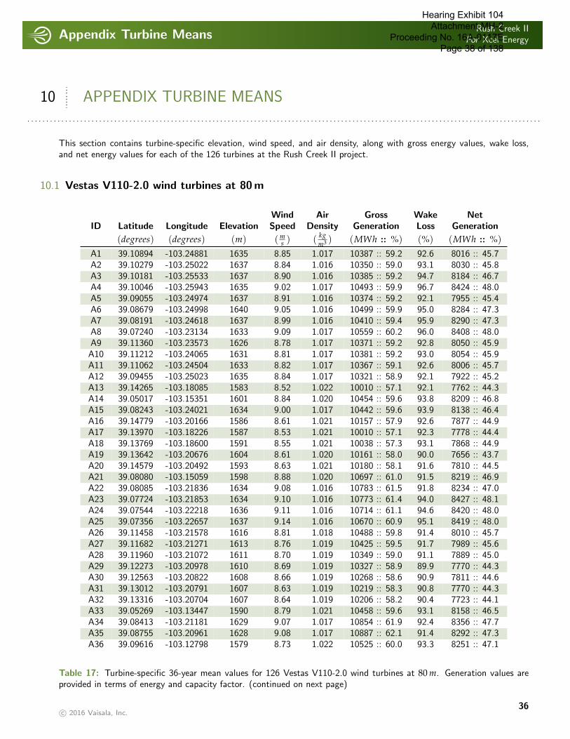
Appendix Turbine MeansRush Creek II
For Xcel Energy
. . . . . . . . . . . . . . . . . . . . . . . . . . . . . . . . . . . . . . . . . . . . . . . . . . . . . . . . . . . . . . . . . . . . . . . . . . . . . . . . . . . . . . . . . . . . . . . . . . . . . . . . . . . . . . . . . .
10 APPENDIX TURBINE MEANS. . . . . . . . . . . . . . . . . . . . . . . . . . . . . . . . . . . . . . . . . . . . . . . . . . . . . . . . . . . . . . . . . . . . . . . . . . . . . . . . . . . . . . . . . . . . . . . . . . . . . . . . . . . . . . . . . . . . . . . . . . . . . . . . . . . . . . . .
This section contains turbine-specific elevation, wind speed, and air density, along with gross energy values, wake loss,and net energy values for each of the 126 turbines at the Rush Creek II project.
10.1 Vestas V110-2.0 wind turbines at 80 m
Wind Air Gross Wake NetID Latitude Longitude Elevation Speed Density Generation Loss Generation
(degrees) (degrees) (m) ( ms ) ( kg
m3 ) (MWh :: %) (%) (MWh :: %)A1 39.10894 -103.24881 1635 8.85 1.017 10387 :: 59.2 92.6 8016 :: 45.7A2 39.10279 -103.25022 1637 8.84 1.016 10350 :: 59.0 93.1 8030 :: 45.8A3 39.10181 -103.25533 1637 8.90 1.016 10385 :: 59.2 94.7 8184 :: 46.7A4 39.10046 -103.25943 1635 9.02 1.017 10493 :: 59.9 96.7 8424 :: 48.0A5 39.09055 -103.24974 1637 8.91 1.016 10374 :: 59.2 92.1 7955 :: 45.4A6 39.08679 -103.24998 1640 9.05 1.016 10499 :: 59.9 95.0 8284 :: 47.3A7 39.08191 -103.24618 1637 8.99 1.016 10410 :: 59.4 95.9 8290 :: 47.3A8 39.07240 -103.23134 1633 9.09 1.017 10559 :: 60.2 96.0 8408 :: 48.0A9 39.11360 -103.23573 1626 8.78 1.017 10371 :: 59.2 92.8 8050 :: 45.9A10 39.11212 -103.24065 1631 8.81 1.017 10381 :: 59.2 93.0 8054 :: 45.9A11 39.11062 -103.24504 1633 8.82 1.017 10367 :: 59.1 92.6 8006 :: 45.7A12 39.09455 -103.25023 1635 8.84 1.017 10321 :: 58.9 92.1 7922 :: 45.2A13 39.14265 -103.18085 1583 8.52 1.022 10010 :: 57.1 92.1 7762 :: 44.3A14 39.05017 -103.15351 1601 8.84 1.020 10454 :: 59.6 93.8 8209 :: 46.8A15 39.08243 -103.24021 1634 9.00 1.017 10442 :: 59.6 93.9 8138 :: 46.4A16 39.14779 -103.20166 1586 8.61 1.021 10157 :: 57.9 92.6 7877 :: 44.9A17 39.13970 -103.18226 1587 8.53 1.021 10010 :: 57.1 92.3 7778 :: 44.4A18 39.13769 -103.18600 1591 8.55 1.021 10038 :: 57.3 93.1 7868 :: 44.9A19 39.13642 -103.20676 1604 8.61 1.020 10161 :: 58.0 90.0 7656 :: 43.7A20 39.14579 -103.20492 1593 8.63 1.021 10180 :: 58.1 91.6 7810 :: 44.5A21 39.08080 -103.15059 1598 8.88 1.020 10697 :: 61.0 91.5 8219 :: 46.9A22 39.08085 -103.21836 1634 9.08 1.016 10783 :: 61.5 91.8 8234 :: 47.0A23 39.07724 -103.21853 1634 9.10 1.016 10773 :: 61.4 94.0 8427 :: 48.1A24 39.07544 -103.22218 1636 9.11 1.016 10714 :: 61.1 94.6 8420 :: 48.0A25 39.07356 -103.22657 1637 9.14 1.016 10670 :: 60.9 95.1 8419 :: 48.0A26 39.11458 -103.21578 1616 8.81 1.018 10488 :: 59.8 91.4 8010 :: 45.7A27 39.11682 -103.21271 1613 8.76 1.019 10425 :: 59.5 91.7 7989 :: 45.6A28 39.11960 -103.21072 1611 8.70 1.019 10349 :: 59.0 91.1 7889 :: 45.0A29 39.12273 -103.20978 1610 8.69 1.019 10327 :: 58.9 89.9 7770 :: 44.3A30 39.12563 -103.20822 1608 8.66 1.019 10268 :: 58.6 90.9 7811 :: 44.6A31 39.13012 -103.20791 1607 8.63 1.019 10219 :: 58.3 90.8 7770 :: 44.3A32 39.13316 -103.20704 1607 8.64 1.019 10206 :: 58.2 90.4 7723 :: 44.1A33 39.05269 -103.13447 1590 8.79 1.021 10458 :: 59.6 93.1 8158 :: 46.5A34 39.08413 -103.21181 1629 9.07 1.017 10854 :: 61.9 92.4 8356 :: 47.7A35 39.08755 -103.20961 1628 9.08 1.017 10887 :: 62.1 91.4 8292 :: 47.3A36 39.09616 -103.12798 1579 8.73 1.022 10525 :: 60.0 93.3 8251 :: 47.1
Table 17: Turbine-specific 36-year mean values for 126 Vestas V110-2.0 wind turbines at 80 m. Generation values areprovided in terms of energy and capacity factor. (continued on next page)
c© 2016 Vaisala, Inc.36
Hearing Exhibit 104 Attachment MH-2
Proceeding No. 16A-0117E Page 38 of 138
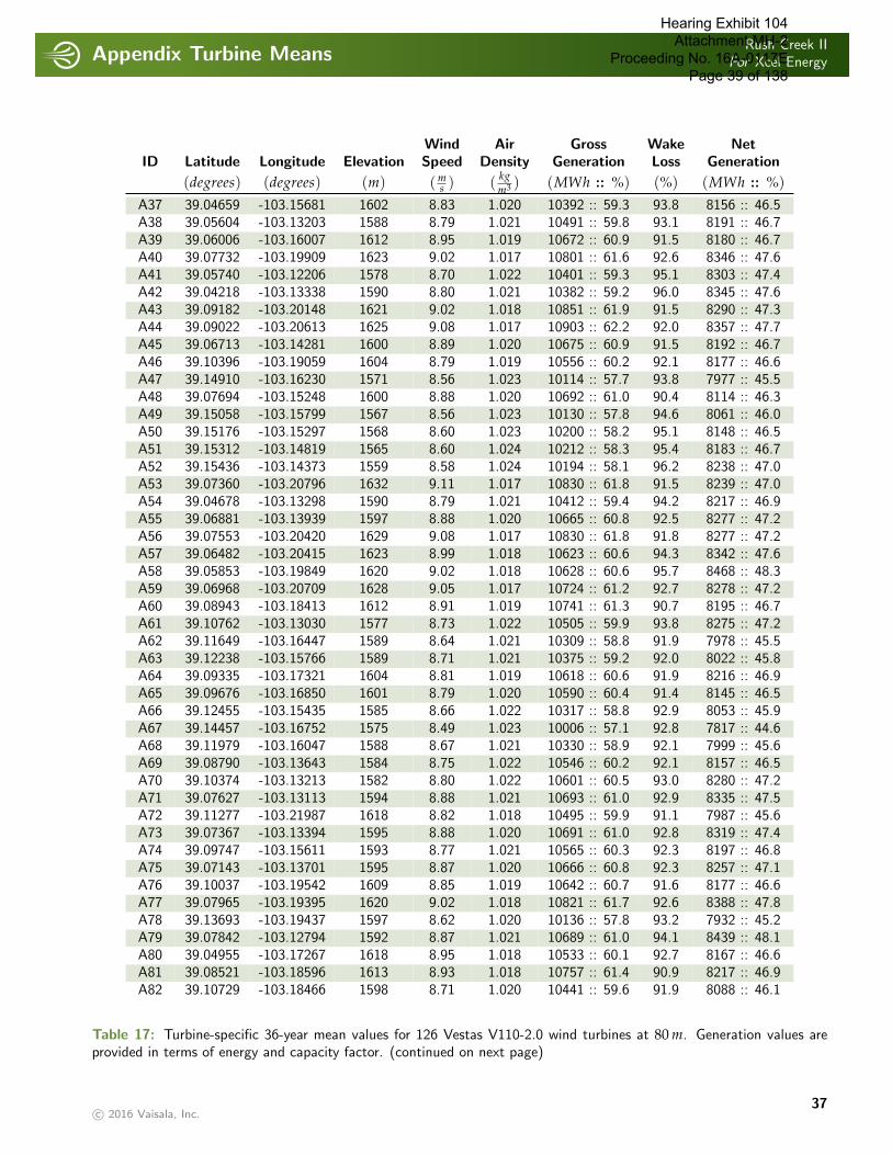
Appendix Turbine MeansRush Creek II
For Xcel Energy
. . . . . . . . . . . . . . . . . . . . . . . . . . . . . . . . . . . . . . . . . . . . . . . . . . . . . . . . . . . . . . . . . . . . . . . . . . . . . . . . . . . . . . . . . . . . . . . . . . . . . . . . . . . . . . . . . .
Wind Air Gross Wake NetID Latitude Longitude Elevation Speed Density Generation Loss Generation
(degrees) (degrees) (m) ( ms ) ( kg
m3 ) (MWh :: %) (%) (MWh :: %)A37 39.04659 -103.15681 1602 8.83 1.020 10392 :: 59.3 93.8 8156 :: 46.5A38 39.05604 -103.13203 1588 8.79 1.021 10491 :: 59.8 93.1 8191 :: 46.7A39 39.06006 -103.16007 1612 8.95 1.019 10672 :: 60.9 91.5 8180 :: 46.7A40 39.07732 -103.19909 1623 9.02 1.017 10801 :: 61.6 92.6 8346 :: 47.6A41 39.05740 -103.12206 1578 8.70 1.022 10401 :: 59.3 95.1 8303 :: 47.4A42 39.04218 -103.13338 1590 8.80 1.021 10382 :: 59.2 96.0 8345 :: 47.6A43 39.09182 -103.20148 1621 9.02 1.018 10851 :: 61.9 91.5 8290 :: 47.3A44 39.09022 -103.20613 1625 9.08 1.017 10903 :: 62.2 92.0 8357 :: 47.7A45 39.06713 -103.14281 1600 8.89 1.020 10675 :: 60.9 91.5 8192 :: 46.7A46 39.10396 -103.19059 1604 8.79 1.019 10556 :: 60.2 92.1 8177 :: 46.6A47 39.14910 -103.16230 1571 8.56 1.023 10114 :: 57.7 93.8 7977 :: 45.5A48 39.07694 -103.15248 1600 8.88 1.020 10692 :: 61.0 90.4 8114 :: 46.3A49 39.15058 -103.15799 1567 8.56 1.023 10130 :: 57.8 94.6 8061 :: 46.0A50 39.15176 -103.15297 1568 8.60 1.023 10200 :: 58.2 95.1 8148 :: 46.5A51 39.15312 -103.14819 1565 8.60 1.024 10212 :: 58.3 95.4 8183 :: 46.7A52 39.15436 -103.14373 1559 8.58 1.024 10194 :: 58.1 96.2 8238 :: 47.0A53 39.07360 -103.20796 1632 9.11 1.017 10830 :: 61.8 91.5 8239 :: 47.0A54 39.04678 -103.13298 1590 8.79 1.021 10412 :: 59.4 94.2 8217 :: 46.9A55 39.06881 -103.13939 1597 8.88 1.020 10665 :: 60.8 92.5 8277 :: 47.2A56 39.07553 -103.20420 1629 9.08 1.017 10830 :: 61.8 91.8 8277 :: 47.2A57 39.06482 -103.20415 1623 8.99 1.018 10623 :: 60.6 94.3 8342 :: 47.6A58 39.05853 -103.19849 1620 9.02 1.018 10628 :: 60.6 95.7 8468 :: 48.3A59 39.06968 -103.20709 1628 9.05 1.017 10724 :: 61.2 92.7 8278 :: 47.2A60 39.08943 -103.18413 1612 8.91 1.019 10741 :: 61.3 90.7 8195 :: 46.7A61 39.10762 -103.13030 1577 8.73 1.022 10505 :: 59.9 93.8 8275 :: 47.2A62 39.11649 -103.16447 1589 8.64 1.021 10309 :: 58.8 91.9 7978 :: 45.5A63 39.12238 -103.15766 1589 8.71 1.021 10375 :: 59.2 92.0 8022 :: 45.8A64 39.09335 -103.17321 1604 8.81 1.019 10618 :: 60.6 91.9 8216 :: 46.9A65 39.09676 -103.16850 1601 8.79 1.020 10590 :: 60.4 91.4 8145 :: 46.5A66 39.12455 -103.15435 1585 8.66 1.022 10317 :: 58.8 92.9 8053 :: 45.9A67 39.14457 -103.16752 1575 8.49 1.023 10006 :: 57.1 92.8 7817 :: 44.6A68 39.11979 -103.16047 1588 8.67 1.021 10330 :: 58.9 92.1 7999 :: 45.6A69 39.08790 -103.13643 1584 8.75 1.022 10546 :: 60.2 92.1 8157 :: 46.5A70 39.10374 -103.13213 1582 8.80 1.022 10601 :: 60.5 93.0 8280 :: 47.2A71 39.07627 -103.13113 1594 8.88 1.021 10693 :: 61.0 92.9 8335 :: 47.5A72 39.11277 -103.21987 1618 8.82 1.018 10495 :: 59.9 91.1 7987 :: 45.6A73 39.07367 -103.13394 1595 8.88 1.020 10691 :: 61.0 92.8 8319 :: 47.4A74 39.09747 -103.15611 1593 8.77 1.021 10565 :: 60.3 92.3 8197 :: 46.8A75 39.07143 -103.13701 1595 8.87 1.020 10666 :: 60.8 92.3 8257 :: 47.1A76 39.10037 -103.19542 1609 8.85 1.019 10642 :: 60.7 91.6 8177 :: 46.6A77 39.07965 -103.19395 1620 9.02 1.018 10821 :: 61.7 92.6 8388 :: 47.8A78 39.13693 -103.19437 1597 8.62 1.020 10136 :: 57.8 93.2 7932 :: 45.2A79 39.07842 -103.12794 1592 8.87 1.021 10689 :: 61.0 94.1 8439 :: 48.1A80 39.04955 -103.17267 1618 8.95 1.018 10533 :: 60.1 92.7 8167 :: 46.6A81 39.08521 -103.18596 1613 8.93 1.018 10757 :: 61.4 90.9 8217 :: 46.9A82 39.10729 -103.18466 1598 8.71 1.020 10441 :: 59.6 91.9 8088 :: 46.1
Table 17: Turbine-specific 36-year mean values for 126 Vestas V110-2.0 wind turbines at 80 m. Generation values areprovided in terms of energy and capacity factor. (continued on next page)
c© 2016 Vaisala, Inc.37
Hearing Exhibit 104 Attachment MH-2
Proceeding No. 16A-0117E Page 39 of 138
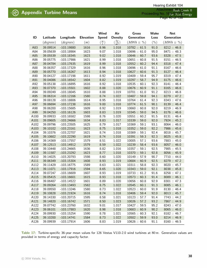
Appendix Turbine MeansRush Creek II
For Xcel Energy
. . . . . . . . . . . . . . . . . . . . . . . . . . . . . . . . . . . . . . . . . . . . . . . . . . . . . . . . . . . . . . . . . . . . . . . . . . . . . . . . . . . . . . . . . . . . . . . . . . . . . . . . . . . . . . . . . .
Wind Air Gross Wake NetID Latitude Longitude Elevation Speed Density Generation Loss Generation
(degrees) (degrees) (m) ( ms ) ( kg
m3 ) (MWh :: %) (%) (MWh :: %)A83 39.09514 -103.19880 1616 8.96 1.018 10782 :: 61.5 91.0 8212 :: 46.8A84 39.05639 -103.18984 1623 9.07 1.018 10696 :: 61.0 95.0 8471 :: 48.3A85 39.05539 -103.18345 1623 9.02 1.018 10646 :: 60.7 93.6 8328 :: 47.5A86 39.05775 -103.17986 1621 8.99 1.018 10651 :: 60.8 91.5 8151 :: 46.5A87 39.04784 -103.17635 1619 8.99 1.018 10552 :: 60.2 94.4 8318 :: 47.4A88 39.06357 -103.17329 1616 8.96 1.018 10696 :: 61.0 91.1 8167 :: 46.6A89 39.05770 -103.16267 1613 8.94 1.018 10627 :: 60.6 91.3 8127 :: 46.4A90 39.04127 -103.17198 1611 8.92 1.019 10409 :: 59.4 95.7 8319 :: 47.4A91 39.04086 -103.16542 1604 8.82 1.019 10297 :: 58.7 94.9 8175 :: 46.6A92 39.05138 -103.16895 1616 8.92 1.018 10535 :: 60.1 92.3 8141 :: 46.4A93 39.07370 -103.15501 1602 8.88 1.020 10676 :: 60.9 91.1 8165 :: 46.6A94 39.09249 -103.18045 1610 8.88 1.019 10701 :: 61.0 91.2 8213 :: 46.8A95 39.06314 -103.12166 1580 8.74 1.022 10487 :: 59.8 94.1 8279 :: 47.2A96 39.08128 -103.18806 1614 8.95 1.018 10764 :: 61.4 92.3 8343 :: 47.6A97 39.06694 -103.17238 1616 9.00 1.018 10774 :: 61.5 90.1 8139 :: 46.4A98 39.06200 -103.15685 1609 8.92 1.019 10660 :: 60.8 92.0 8219 :: 46.9A99 39.04250 -103.16126 1603 8.83 1.019 10345 :: 59.0 94.5 8176 :: 46.6A100 39.09933 -103.16582 1598 8.76 1.020 10551 :: 60.2 91.5 8131 :: 46.4A101 39.09605 -103.24666 1634 8.83 1.017 10339 :: 59.0 92.0 7924 :: 45.2A102 39.09796 -103.23505 1625 8.79 1.017 10369 :: 59.1 93.1 8064 :: 46.0A103 39.10102 -103.23161 1623 8.75 1.018 10352 :: 59.0 92.2 7986 :: 45.6A104 39.10376 -103.22707 1621 8.74 1.018 10369 :: 59.1 92.4 8018 :: 45.7A105 39.10602 -103.22290 1619 8.74 1.018 10391 :: 59.3 92.3 8025 :: 45.8A106 39.14369 -103.17557 1579 8.51 1.022 10005 :: 57.1 93.6 7883 :: 45.0A107 39.12513 -103.14912 1579 8.59 1.022 10239 :: 58.4 93.6 8057 :: 46.0A108 39.10448 -103.24665 1636 8.82 1.016 10357 :: 59.1 92.5 7985 :: 45.5A109 39.11587 -103.23292 1623 8.77 1.018 10370 :: 59.1 92.8 8056 :: 45.9A110 39.14025 -103.20793 1598 8.60 1.020 10149 :: 57.9 90.7 7710 :: 44.0A111 39.06349 -103.15304 1608 8.93 1.019 10684 :: 60.9 92.5 8279 :: 47.2A112 39.11429 -103.16775 1589 8.63 1.021 10311 :: 58.8 92.3 8020 :: 45.7A113 39.11071 -103.17916 1594 8.65 1.020 10343 :: 59.0 92.1 8038 :: 45.8A114 39.07247 -103.16609 1607 8.93 1.019 10733 :: 61.2 91.6 8258 :: 47.1A115 39.05415 -103.16601 1615 8.93 1.018 10573 :: 60.3 91.4 8089 :: 46.1A116 39.06487 -103.14522 1601 8.89 1.020 10656 :: 60.8 92.9 8301 :: 47.3A117 39.09264 -103.13493 1582 8.75 1.022 10545 :: 60.1 91.3 8085 :: 46.1A118 39.09550 -103.13246 1580 8.73 1.022 10523 :: 60.0 91.9 8130 :: 46.4A119 39.10828 -103.21924 1616 8.74 1.018 10406 :: 59.4 92.0 8013 :: 45.7A120 39.14330 -103.20715 1595 8.58 1.021 10123 :: 57.7 91.4 7743 :: 44.2A121 39.14820 -103.16742 1571 8.50 1.023 10026 :: 57.2 93.2 7867 :: 44.9A122 39.07742 -103.23760 1632 9.01 1.017 10427 :: 59.5 95.2 8243 :: 47.0A123 39.06101 -103.17883 1620 8.98 1.018 10683 :: 60.9 90.2 8065 :: 46.0A124 39.09930 -103.15254 1590 8.78 1.021 10565 :: 60.3 92.1 8182 :: 46.7A125 39.10200 -103.14741 1584 8.73 1.022 10502 :: 59.9 93.0 8214 :: 46.9A126 39.09939 -103.17914 1606 8.83 1.019 10626 :: 60.6 91.1 8160 :: 46.5
Table 17: Turbine-specific 36-year mean values for 126 Vestas V110-2.0 wind turbines at 80 m. Generation values areprovided in terms of energy and capacity factor.
c© 2016 Vaisala, Inc.38
Hearing Exhibit 104 Attachment MH-2
Proceeding No. 16A-0117E Page 40 of 138
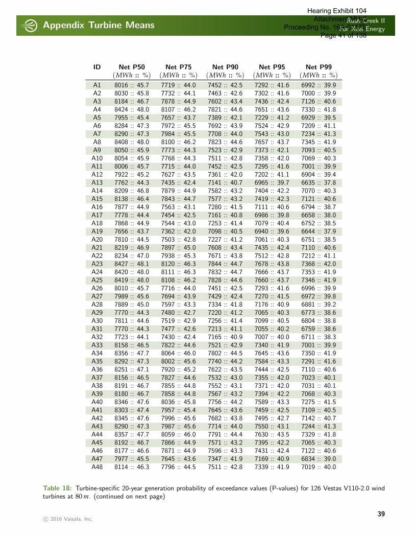
Appendix Turbine MeansRush Creek II
For Xcel Energy
. . . . . . . . . . . . . . . . . . . . . . . . . . . . . . . . . . . . . . . . . . . . . . . . . . . . . . . . . . . . . . . . . . . . . . . . . . . . . . . . . . . . . . . . . . . . . . . . . . . . . . . . . . . . . . . . . .
ID Net P50 Net P75 Net P90 Net P95 Net P99(MWh :: %) (MWh :: %) (MWh :: %) (MWh :: %) (MWh :: %)
A1 8016 :: 45.7 7719 :: 44.0 7452 :: 42.5 7292 :: 41.6 6992 :: 39.9A2 8030 :: 45.8 7732 :: 44.1 7463 :: 42.6 7302 :: 41.6 7000 :: 39.9A3 8184 :: 46.7 7878 :: 44.9 7602 :: 43.4 7436 :: 42.4 7126 :: 40.6A4 8424 :: 48.0 8107 :: 46.2 7821 :: 44.6 7651 :: 43.6 7330 :: 41.8A5 7955 :: 45.4 7657 :: 43.7 7389 :: 42.1 7229 :: 41.2 6929 :: 39.5A6 8284 :: 47.3 7972 :: 45.5 7692 :: 43.9 7524 :: 42.9 7209 :: 41.1A7 8290 :: 47.3 7984 :: 45.5 7708 :: 44.0 7543 :: 43.0 7234 :: 41.3A8 8408 :: 48.0 8100 :: 46.2 7823 :: 44.6 7657 :: 43.7 7345 :: 41.9A9 8050 :: 45.9 7773 :: 44.3 7523 :: 42.9 7373 :: 42.1 7093 :: 40.5A10 8054 :: 45.9 7768 :: 44.3 7511 :: 42.8 7358 :: 42.0 7069 :: 40.3A11 8006 :: 45.7 7715 :: 44.0 7452 :: 42.5 7295 :: 41.6 7001 :: 39.9A12 7922 :: 45.2 7627 :: 43.5 7361 :: 42.0 7202 :: 41.1 6904 :: 39.4A13 7762 :: 44.3 7435 :: 42.4 7141 :: 40.7 6965 :: 39.7 6635 :: 37.8A14 8209 :: 46.8 7879 :: 44.9 7582 :: 43.2 7404 :: 42.2 7070 :: 40.3A15 8138 :: 46.4 7843 :: 44.7 7577 :: 43.2 7419 :: 42.3 7121 :: 40.6A16 7877 :: 44.9 7563 :: 43.1 7280 :: 41.5 7111 :: 40.6 6794 :: 38.7A17 7778 :: 44.4 7454 :: 42.5 7161 :: 40.8 6986 :: 39.8 6658 :: 38.0A18 7868 :: 44.9 7544 :: 43.0 7253 :: 41.4 7079 :: 40.4 6752 :: 38.5A19 7656 :: 43.7 7362 :: 42.0 7098 :: 40.5 6940 :: 39.6 6644 :: 37.9A20 7810 :: 44.5 7503 :: 42.8 7227 :: 41.2 7061 :: 40.3 6751 :: 38.5A21 8219 :: 46.9 7897 :: 45.0 7608 :: 43.4 7435 :: 42.4 7110 :: 40.6A22 8234 :: 47.0 7938 :: 45.3 7671 :: 43.8 7512 :: 42.8 7212 :: 41.1A23 8427 :: 48.1 8120 :: 46.3 7844 :: 44.7 7678 :: 43.8 7368 :: 42.0A24 8420 :: 48.0 8111 :: 46.3 7832 :: 44.7 7666 :: 43.7 7353 :: 41.9A25 8419 :: 48.0 8108 :: 46.2 7828 :: 44.6 7660 :: 43.7 7346 :: 41.9A26 8010 :: 45.7 7716 :: 44.0 7451 :: 42.5 7293 :: 41.6 6996 :: 39.9A27 7989 :: 45.6 7694 :: 43.9 7429 :: 42.4 7270 :: 41.5 6972 :: 39.8A28 7889 :: 45.0 7597 :: 43.3 7334 :: 41.8 7176 :: 40.9 6881 :: 39.2A29 7770 :: 44.3 7480 :: 42.7 7220 :: 41.2 7065 :: 40.3 6773 :: 38.6A30 7811 :: 44.6 7519 :: 42.9 7256 :: 41.4 7099 :: 40.5 6804 :: 38.8A31 7770 :: 44.3 7477 :: 42.6 7213 :: 41.1 7055 :: 40.2 6759 :: 38.6A32 7723 :: 44.1 7430 :: 42.4 7165 :: 40.9 7007 :: 40.0 6711 :: 38.3A33 8158 :: 46.5 7822 :: 44.6 7521 :: 42.9 7340 :: 41.9 7001 :: 39.9A34 8356 :: 47.7 8064 :: 46.0 7802 :: 44.5 7645 :: 43.6 7350 :: 41.9A35 8292 :: 47.3 8002 :: 45.6 7740 :: 44.2 7584 :: 43.3 7291 :: 41.6A36 8251 :: 47.1 7920 :: 45.2 7622 :: 43.5 7444 :: 42.5 7110 :: 40.6A37 8156 :: 46.5 7827 :: 44.6 7532 :: 43.0 7355 :: 42.0 7023 :: 40.1A38 8191 :: 46.7 7855 :: 44.8 7552 :: 43.1 7371 :: 42.0 7031 :: 40.1A39 8180 :: 46.7 7858 :: 44.8 7567 :: 43.2 7394 :: 42.2 7068 :: 40.3A40 8346 :: 47.6 8036 :: 45.8 7756 :: 44.2 7589 :: 43.3 7275 :: 41.5A41 8303 :: 47.4 7957 :: 45.4 7645 :: 43.6 7459 :: 42.5 7109 :: 40.5A42 8345 :: 47.6 7996 :: 45.6 7682 :: 43.8 7495 :: 42.7 7142 :: 40.7A43 8290 :: 47.3 7987 :: 45.6 7714 :: 44.0 7550 :: 43.1 7244 :: 41.3A44 8357 :: 47.7 8059 :: 46.0 7791 :: 44.4 7630 :: 43.5 7329 :: 41.8A45 8192 :: 46.7 7866 :: 44.9 7571 :: 43.2 7395 :: 42.2 7065 :: 40.3A46 8177 :: 46.6 7871 :: 44.9 7596 :: 43.3 7431 :: 42.4 7122 :: 40.6A47 7977 :: 45.5 7645 :: 43.6 7347 :: 41.9 7169 :: 40.9 6834 :: 39.0A48 8114 :: 46.3 7796 :: 44.5 7511 :: 42.8 7339 :: 41.9 7019 :: 40.0
Table 18: Turbine-specific 20-year generation probability of exceedance values (P-values) for 126 Vestas V110-2.0 windturbines at 80 m. (continued on next page)
c© 2016 Vaisala, Inc.39
Hearing Exhibit 104 Attachment MH-2
Proceeding No. 16A-0117E Page 41 of 138
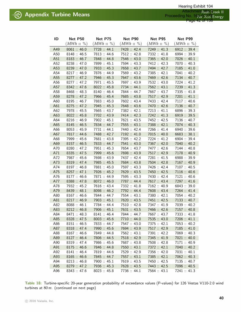
Appendix Turbine MeansRush Creek II
For Xcel Energy
. . . . . . . . . . . . . . . . . . . . . . . . . . . . . . . . . . . . . . . . . . . . . . . . . . . . . . . . . . . . . . . . . . . . . . . . . . . . . . . . . . . . . . . . . . . . . . . . . . . . . . . . . . . . . . . . . .
ID Net P50 Net P75 Net P90 Net P95 Net P99(MWh :: %) (MWh :: %) (MWh :: %) (MWh :: %) (MWh :: %)
A49 8061 :: 46.0 7728 :: 44.1 7428 :: 42.4 7249 :: 41.3 6912 :: 39.4A50 8148 :: 46.5 7813 :: 44.6 7512 :: 42.8 7332 :: 41.8 6994 :: 39.9A51 8183 :: 46.7 7848 :: 44.8 7546 :: 43.0 7365 :: 42.0 7026 :: 40.1A52 8238 :: 47.0 7899 :: 45.1 7594 :: 43.3 7412 :: 42.3 7070 :: 40.3A53 8239 :: 47.0 7933 :: 45.3 7658 :: 43.7 7494 :: 42.7 7185 :: 41.0A54 8217 :: 46.9 7876 :: 44.9 7569 :: 43.2 7385 :: 42.1 7041 :: 40.2A55 8277 :: 47.2 7946 :: 45.3 7647 :: 43.6 7469 :: 42.6 7134 :: 40.7A56 8277 :: 47.2 7971 :: 45.5 7697 :: 43.9 7532 :: 43.0 7224 :: 41.2A57 8342 :: 47.6 8022 :: 45.8 7734 :: 44.1 7562 :: 43.1 7239 :: 41.3A58 8468 :: 48.3 8140 :: 46.4 7844 :: 44.7 7667 :: 43.7 7335 :: 41.8A59 8278 :: 47.2 7966 :: 45.4 7685 :: 43.8 7517 :: 42.9 7201 :: 41.1A60 8195 :: 46.7 7883 :: 45.0 7602 :: 43.4 7433 :: 42.4 7117 :: 40.6A61 8275 :: 47.2 7945 :: 45.3 7648 :: 43.6 7470 :: 42.6 7136 :: 40.7A62 7978 :: 45.5 7665 :: 43.7 7382 :: 42.1 7213 :: 41.1 6896 :: 39.3A63 8022 :: 45.8 7702 :: 43.9 7414 :: 42.3 7242 :: 41.3 6919 :: 39.5A64 8216 :: 46.9 7902 :: 45.1 7621 :: 43.5 7452 :: 42.5 7136 :: 40.7A65 8145 :: 46.5 7834 :: 44.7 7555 :: 43.1 7388 :: 42.1 7074 :: 40.3A66 8053 :: 45.9 7731 :: 44.1 7440 :: 42.4 7266 :: 41.4 6940 :: 39.6A67 7817 :: 44.6 7488 :: 42.7 7192 :: 41.0 7015 :: 40.0 6683 :: 38.1A68 7999 :: 45.6 7681 :: 43.8 7395 :: 42.2 7224 :: 41.2 6904 :: 39.4A69 8157 :: 46.5 7833 :: 44.7 7541 :: 43.0 7367 :: 42.0 7040 :: 40.2A70 8280 :: 47.2 7951 :: 45.3 7654 :: 43.7 7477 :: 42.6 7144 :: 40.8A71 8335 :: 47.5 7999 :: 45.6 7698 :: 43.9 7517 :: 42.9 7178 :: 40.9A72 7987 :: 45.6 7698 :: 43.9 7437 :: 42.4 7281 :: 41.5 6988 :: 39.9A73 8319 :: 47.4 7985 :: 45.5 7684 :: 43.8 7504 :: 42.8 7167 :: 40.9A74 8197 :: 46.8 7881 :: 45.0 7597 :: 43.3 7426 :: 42.4 7107 :: 40.5A75 8257 :: 47.1 7926 :: 45.2 7629 :: 43.5 7450 :: 42.5 7116 :: 40.6A76 8177 :: 46.6 7871 :: 44.9 7595 :: 43.3 7430 :: 42.4 7121 :: 40.6A77 8388 :: 47.8 8072 :: 46.0 7787 :: 44.4 7617 :: 43.4 7297 :: 41.6A78 7932 :: 45.2 7616 :: 43.4 7332 :: 41.8 7162 :: 40.9 6843 :: 39.0A79 8439 :: 48.1 8098 :: 46.2 7792 :: 44.4 7608 :: 43.4 7264 :: 41.4A80 8167 :: 46.6 7844 :: 44.7 7554 :: 43.1 7380 :: 42.1 7054 :: 40.2A81 8217 :: 46.9 7903 :: 45.1 7620 :: 43.5 7451 :: 42.5 7133 :: 40.7A82 8088 :: 46.1 7784 :: 44.4 7510 :: 42.8 7347 :: 41.9 7039 :: 40.2A83 8212 :: 46.8 7906 :: 45.1 7631 :: 43.5 7466 :: 42.6 7157 :: 40.8A84 8471 :: 48.3 8141 :: 46.4 7844 :: 44.7 7667 :: 43.7 7333 :: 41.8A85 8328 :: 47.5 8003 :: 45.6 7710 :: 44.0 7535 :: 43.0 7206 :: 41.1A86 8151 :: 46.5 7833 :: 44.7 7547 :: 43.0 7375 :: 42.1 7053 :: 40.2A87 8318 :: 47.4 7990 :: 45.6 7694 :: 43.9 7517 :: 42.9 7185 :: 41.0A88 8167 :: 46.6 7849 :: 44.8 7562 :: 43.1 7391 :: 42.2 7069 :: 40.3A89 8127 :: 46.4 7806 :: 44.5 7518 :: 42.9 7345 :: 41.9 7021 :: 40.0A90 8319 :: 47.4 7986 :: 45.6 7687 :: 43.8 7508 :: 42.8 7171 :: 40.9A91 8175 :: 46.6 7846 :: 44.8 7550 :: 43.1 7372 :: 42.1 7040 :: 40.2A92 8141 :: 46.4 7819 :: 44.6 7529 :: 42.9 7356 :: 42.0 7031 :: 40.1A93 8165 :: 46.6 7845 :: 44.7 7557 :: 43.1 7385 :: 42.1 7062 :: 40.3A94 8213 :: 46.8 7900 :: 45.1 7619 :: 43.5 7450 :: 42.5 7135 :: 40.7A95 8279 :: 47.2 7936 :: 45.3 7628 :: 43.5 7443 :: 42.5 7096 :: 40.5A96 8343 :: 47.6 8023 :: 45.8 7736 :: 44.1 7564 :: 43.1 7241 :: 41.3
Table 18: Turbine-specific 20-year generation probability of exceedance values (P-values) for 126 Vestas V110-2.0 windturbines at 80 m. (continued on next page)
c© 2016 Vaisala, Inc.40
Hearing Exhibit 104 Attachment MH-2
Proceeding No. 16A-0117E Page 42 of 138
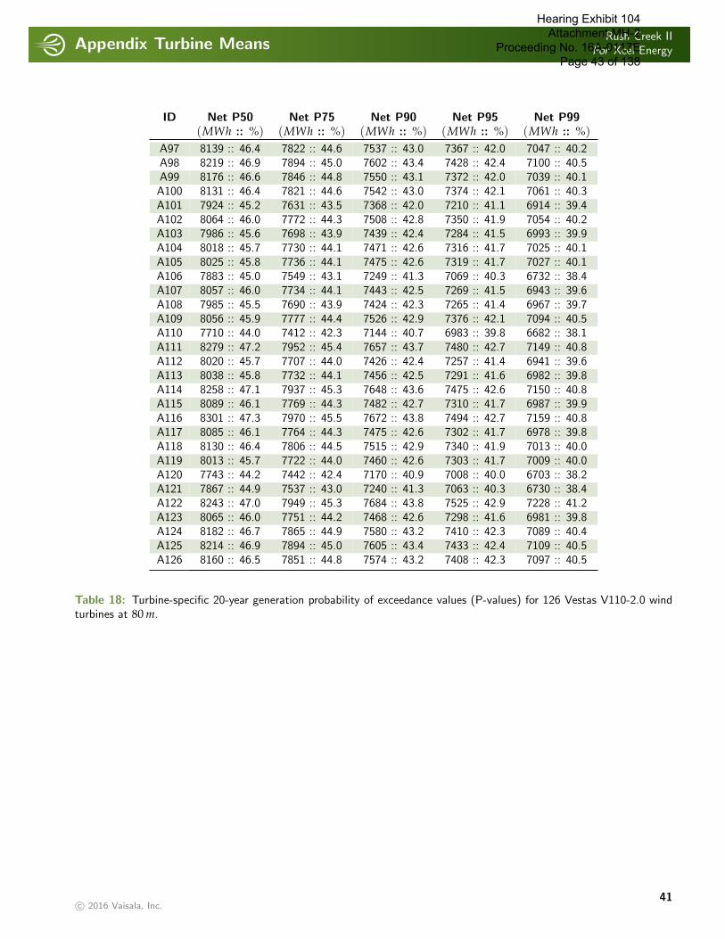
Appendix Turbine MeansRush Creek II
For Xcel Energy
. . . . . . . . . . . . . . . . . . . . . . . . . . . . . . . . . . . . . . . . . . . . . . . . . . . . . . . . . . . . . . . . . . . . . . . . . . . . . . . . . . . . . . . . . . . . . . . . . . . . . . . . . . . . . . . . . .
ID Net P50 Net P75 Net P90 Net P95 Net P99(MWh :: %) (MWh :: %) (MWh :: %) (MWh :: %) (MWh :: %)
A97 8139 :: 46.4 7822 :: 44.6 7537 :: 43.0 7367 :: 42.0 7047 :: 40.2A98 8219 :: 46.9 7894 :: 45.0 7602 :: 43.4 7428 :: 42.4 7100 :: 40.5A99 8176 :: 46.6 7846 :: 44.8 7550 :: 43.1 7372 :: 42.0 7039 :: 40.1A100 8131 :: 46.4 7821 :: 44.6 7542 :: 43.0 7374 :: 42.1 7061 :: 40.3A101 7924 :: 45.2 7631 :: 43.5 7368 :: 42.0 7210 :: 41.1 6914 :: 39.4A102 8064 :: 46.0 7772 :: 44.3 7508 :: 42.8 7350 :: 41.9 7054 :: 40.2A103 7986 :: 45.6 7698 :: 43.9 7439 :: 42.4 7284 :: 41.5 6993 :: 39.9A104 8018 :: 45.7 7730 :: 44.1 7471 :: 42.6 7316 :: 41.7 7025 :: 40.1A105 8025 :: 45.8 7736 :: 44.1 7475 :: 42.6 7319 :: 41.7 7027 :: 40.1A106 7883 :: 45.0 7549 :: 43.1 7249 :: 41.3 7069 :: 40.3 6732 :: 38.4A107 8057 :: 46.0 7734 :: 44.1 7443 :: 42.5 7269 :: 41.5 6943 :: 39.6A108 7985 :: 45.5 7690 :: 43.9 7424 :: 42.3 7265 :: 41.4 6967 :: 39.7A109 8056 :: 45.9 7777 :: 44.4 7526 :: 42.9 7376 :: 42.1 7094 :: 40.5A110 7710 :: 44.0 7412 :: 42.3 7144 :: 40.7 6983 :: 39.8 6682 :: 38.1A111 8279 :: 47.2 7952 :: 45.4 7657 :: 43.7 7480 :: 42.7 7149 :: 40.8A112 8020 :: 45.7 7707 :: 44.0 7426 :: 42.4 7257 :: 41.4 6941 :: 39.6A113 8038 :: 45.8 7732 :: 44.1 7456 :: 42.5 7291 :: 41.6 6982 :: 39.8A114 8258 :: 47.1 7937 :: 45.3 7648 :: 43.6 7475 :: 42.6 7150 :: 40.8A115 8089 :: 46.1 7769 :: 44.3 7482 :: 42.7 7310 :: 41.7 6987 :: 39.9A116 8301 :: 47.3 7970 :: 45.5 7672 :: 43.8 7494 :: 42.7 7159 :: 40.8A117 8085 :: 46.1 7764 :: 44.3 7475 :: 42.6 7302 :: 41.7 6978 :: 39.8A118 8130 :: 46.4 7806 :: 44.5 7515 :: 42.9 7340 :: 41.9 7013 :: 40.0A119 8013 :: 45.7 7722 :: 44.0 7460 :: 42.6 7303 :: 41.7 7009 :: 40.0A120 7743 :: 44.2 7442 :: 42.4 7170 :: 40.9 7008 :: 40.0 6703 :: 38.2A121 7867 :: 44.9 7537 :: 43.0 7240 :: 41.3 7063 :: 40.3 6730 :: 38.4A122 8243 :: 47.0 7949 :: 45.3 7684 :: 43.8 7525 :: 42.9 7228 :: 41.2A123 8065 :: 46.0 7751 :: 44.2 7468 :: 42.6 7298 :: 41.6 6981 :: 39.8A124 8182 :: 46.7 7865 :: 44.9 7580 :: 43.2 7410 :: 42.3 7089 :: 40.4A125 8214 :: 46.9 7894 :: 45.0 7605 :: 43.4 7433 :: 42.4 7109 :: 40.5A126 8160 :: 46.5 7851 :: 44.8 7574 :: 43.2 7408 :: 42.3 7097 :: 40.5
Table 18: Turbine-specific 20-year generation probability of exceedance values (P-values) for 126 Vestas V110-2.0 windturbines at 80 m.
c© 2016 Vaisala, Inc.41
Hearing Exhibit 104 Attachment MH-2
Proceeding No. 16A-0117E Page 43 of 138
Appendix Gross Long-term VariabilityRush Creek II
For Xcel Energy
. . . . . . . . . . . . . . . . . . . . . . . . . . . . . . . . . . . . . . . . . . . . . . . . . . . . . . . . . . . . . . . . . . . . . . . . . . . . . . . . . . . . . . . . . . . . . . . . . . . . . . . . . . . . . . . . . .
11 APPENDIX GROSS LONG-TERM VARIABILITY. . . . . . . . . . . . . . . . . . . . . . . . . . . . . . . . . . . . . . . . . . . . . . . . . . . . . . . . . . . . . . . . . . . . . . . . . . . . . . . . . . . . . . . . . . . . . . . . . . . . . . . . . . . . . . . . . . . . . . . . . . . . . . . . . . . . . . . .
11.1 Summary
This section provides a retrospective analysis of the past 36 years of wind speed and power at the Rush Creek II location.These data were derived from a mesoscale Numerical Weather Prediction (NWP) model that has been statistically calibratedto match the observed data during the measurement period at each meteorological tower for which data were provided(Towers M2196, M2202, M2311 and M2313). Due to long-term climate variability and/or change the historic distributionsof wind and power capacity described here may not be indicative of future conditions.
Based on the results of 3TIER’s Energy Risk Framework, the last 36 years (January, 1980 – December, 2015) of data havebeen utilized for estimating the expected future generation at Rush Creek II. The average MOS-corrected simulated windspeed at hub height (80 m) during the past 36 years of record (January, 1980 – December, 2015) across all 126 turbinesis 8.83 m/s. The average MOS-corrected simulated gross power capacity at hub height during the past 36 years acrossall 126 turbines is 59.8%. A map of average MOS-corrected gross power capacity values across the Rush Creek II projectarea using the power curve for the Vestas V110-2.0 wind turbines is displayed in Power Capacity Maps.
All power capacities presented in this section are gross power capacities.
c© 2016 Vaisala, Inc.42
Hearing Exhibit 104 Attachment MH-2
Proceeding No. 16A-0117E Page 44 of 138
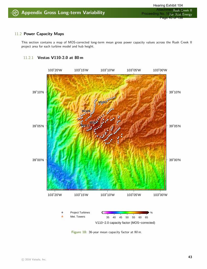
Appendix Gross Long-term VariabilityRush Creek II
For Xcel Energy
. . . . . . . . . . . . . . . . . . . . . . . . . . . . . . . . . . . . . . . . . . . . . . . . . . . . . . . . . . . . . . . . . . . . . . . . . . . . . . . . . . . . . . . . . . . . . . . . . . . . . . . . . . . . . . . . . .
11.2 Power Capacity Maps
This section contains a map of MOS-corrected long-term mean gross power capacity values across the Rush Creek IIproject area for each turbine model and hub height.
11.2.1 Vestas V110-2.0 at 80 m
103˚20'W
103˚20'W
103˚15'W
103˚15'W
103˚10'W
103˚10'W
103˚05'W
103˚05'W
103˚00'W
103˚00'W
39˚00'N 39˚00'N
39˚05'N 39˚05'N
39˚10'N 39˚10'N
M2196
M2202
M2311M2313
35 40 45 50 55 60 65
V110−2.0 capacity factor (MOS−corrected)
%Project Turbines
Met. Towers
Figure 18: 36-year mean capacity factor at 80 m.
c© 2016 Vaisala, Inc.43
Hearing Exhibit 104 Attachment MH-2
Proceeding No. 16A-0117E Page 45 of 138
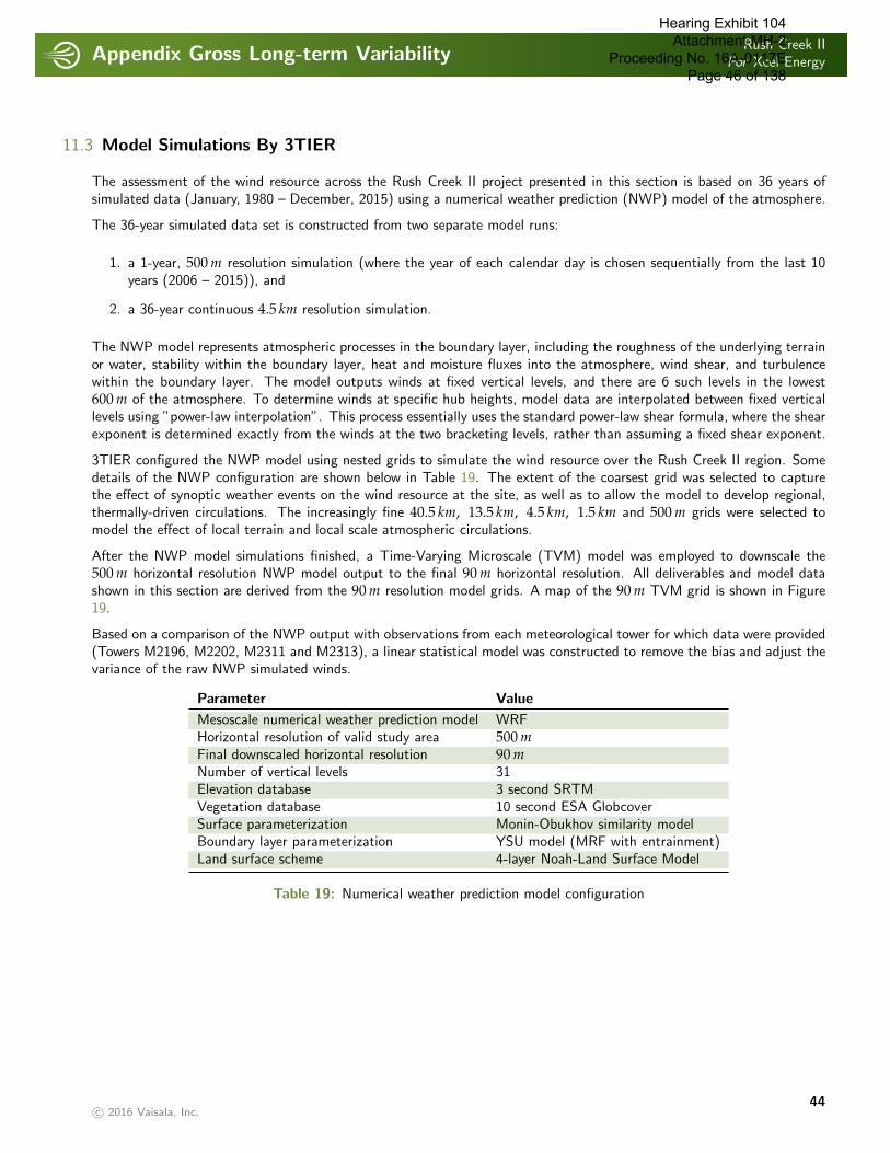
Appendix Gross Long-term VariabilityRush Creek II
For Xcel Energy
. . . . . . . . . . . . . . . . . . . . . . . . . . . . . . . . . . . . . . . . . . . . . . . . . . . . . . . . . . . . . . . . . . . . . . . . . . . . . . . . . . . . . . . . . . . . . . . . . . . . . . . . . . . . . . . . . .
11.3 Model Simulations By 3TIER
The assessment of the wind resource across the Rush Creek II project presented in this section is based on 36 years ofsimulated data (January, 1980 – December, 2015) using a numerical weather prediction (NWP) model of the atmosphere.
The 36-year simulated data set is constructed from two separate model runs:
1. a 1-year, 500 m resolution simulation (where the year of each calendar day is chosen sequentially from the last 10years (2006 – 2015)), and
2. a 36-year continuous 4.5 km resolution simulation.
The NWP model represents atmospheric processes in the boundary layer, including the roughness of the underlying terrainor water, stability within the boundary layer, heat and moisture fluxes into the atmosphere, wind shear, and turbulencewithin the boundary layer. The model outputs winds at fixed vertical levels, and there are 6 such levels in the lowest600 m of the atmosphere. To determine winds at specific hub heights, model data are interpolated between fixed verticallevels using ”power-law interpolation”. This process essentially uses the standard power-law shear formula, where the shearexponent is determined exactly from the winds at the two bracketing levels, rather than assuming a fixed shear exponent.
3TIER configured the NWP model using nested grids to simulate the wind resource over the Rush Creek II region. Somedetails of the NWP configuration are shown below in Table 19. The extent of the coarsest grid was selected to capturethe effect of synoptic weather events on the wind resource at the site, as well as to allow the model to develop regional,thermally-driven circulations. The increasingly fine 40.5 km, 13.5 km, 4.5 km, 1.5 km and 500 m grids were selected tomodel the effect of local terrain and local scale atmospheric circulations.
After the NWP model simulations finished, a Time-Varying Microscale (TVM) model was employed to downscale the500 m horizontal resolution NWP model output to the final 90 m horizontal resolution. All deliverables and model datashown in this section are derived from the 90 m resolution model grids. A map of the 90 m TVM grid is shown in Figure19.
Based on a comparison of the NWP output with observations from each meteorological tower for which data were provided(Towers M2196, M2202, M2311 and M2313), a linear statistical model was constructed to remove the bias and adjust thevariance of the raw NWP simulated winds.
Parameter Value
Mesoscale numerical weather prediction model WRFHorizontal resolution of valid study area 500 mFinal downscaled horizontal resolution 90 mNumber of vertical levels 31Elevation database 3 second SRTMVegetation database 10 second ESA GlobcoverSurface parameterization Monin-Obukhov similarity modelBoundary layer parameterization YSU model (MRF with entrainment)Land surface scheme 4-layer Noah-Land Surface Model
Table 19: Numerical weather prediction model configuration
c© 2016 Vaisala, Inc.44
Hearing Exhibit 104 Attachment MH-2
Proceeding No. 16A-0117E Page 46 of 138
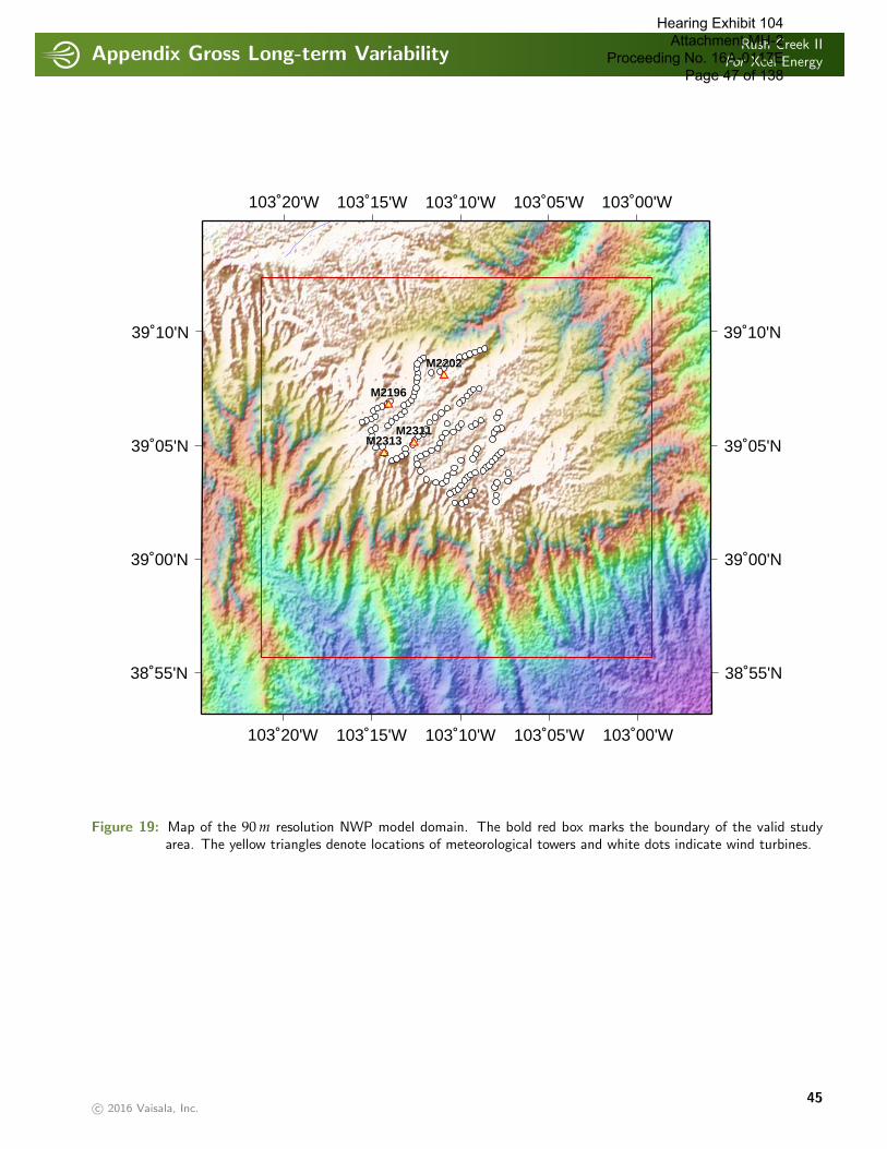
Appendix Gross Long-term VariabilityRush Creek II
For Xcel Energy
. . . . . . . . . . . . . . . . . . . . . . . . . . . . . . . . . . . . . . . . . . . . . . . . . . . . . . . . . . . . . . . . . . . . . . . . . . . . . . . . . . . . . . . . . . . . . . . . . . . . . . . . . . . . . . . . . .
103˚20'W
103˚20'W
103˚15'W
103˚15'W
103˚10'W
103˚10'W
103˚05'W
103˚05'W
103˚00'W
103˚00'W
38˚55'N 38˚55'N
39˚00'N 39˚00'N
39˚05'N 39˚05'N
39˚10'N 39˚10'N
M2196
M2202
M2311M2313
Figure 19: Map of the 90 m resolution NWP model domain. The bold red box marks the boundary of the valid studyarea. The yellow triangles denote locations of meteorological towers and white dots indicate wind turbines.
c© 2016 Vaisala, Inc.45
Hearing Exhibit 104 Attachment MH-2
Proceeding No. 16A-0117E Page 47 of 138
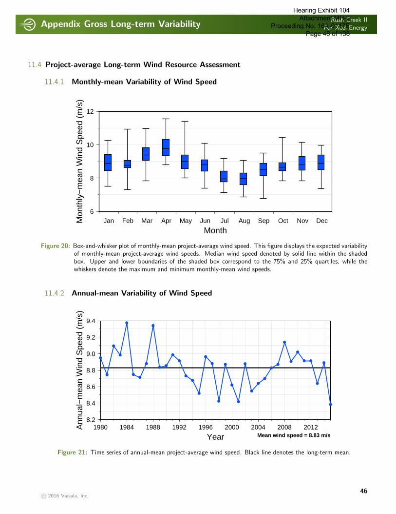
Appendix Gross Long-term VariabilityRush Creek II
For Xcel Energy
. . . . . . . . . . . . . . . . . . . . . . . . . . . . . . . . . . . . . . . . . . . . . . . . . . . . . . . . . . . . . . . . . . . . . . . . . . . . . . . . . . . . . . . . . . . . . . . . . . . . . . . . . . . . . . . . . .
11.4 Project-average Long-term Wind Resource Assessment
11.4.1 Monthly-mean Variability of Wind Speed
Jan Feb Mar Apr May Jun Jul Aug Sep Oct Nov Dec
Month
6
8
10
12
Mon
thly
−m
ean
Win
d S
peed
(m
/s)
Figure 20: Box-and-whisker plot of monthly-mean project-average wind speed. This figure displays the expected variabilityof monthly-mean project-average wind speeds. Median wind speed denoted by solid line within the shadedbox. Upper and lower boundaries of the shaded box correspond to the 75% and 25% quartiles, while thewhiskers denote the maximum and minimum monthly-mean wind speeds.
11.4.2 Annual-mean Variability of Wind Speed
8.2
8.4
8.6
8.8
9.0
9.2
9.4
Ann
ual−
mea
n W
ind
Spe
ed (
m/s
)
1980 1984 1988 1992 1996 2000 2004 2008 2012
Year Mean wind speed = 8.83 m/s
Figure 21: Time series of annual-mean project-average wind speed. Black line denotes the long-term mean.
c© 2016 Vaisala, Inc.46
Hearing Exhibit 104 Attachment MH-2
Proceeding No. 16A-0117E Page 48 of 138
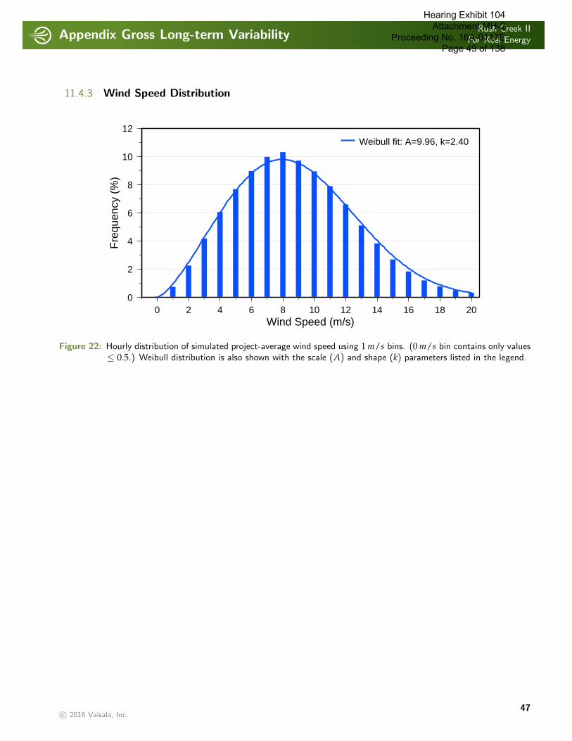
Appendix Gross Long-term VariabilityRush Creek II
For Xcel Energy
. . . . . . . . . . . . . . . . . . . . . . . . . . . . . . . . . . . . . . . . . . . . . . . . . . . . . . . . . . . . . . . . . . . . . . . . . . . . . . . . . . . . . . . . . . . . . . . . . . . . . . . . . . . . . . . . . .
11.4.3 Wind Speed Distribution
0 2 4 6 8 10 12 14 16 18 20Wind Speed (m/s)
0
2
4
6
8
10
12
Fre
quen
cy (
%)
Weibull fit: A=9.96, k=2.40
Figure 22: Hourly distribution of simulated project-average wind speed using 1 m/s bins. (0 m/s bin contains only values≤ 0.5.) Weibull distribution is also shown with the scale (A) and shape (k) parameters listed in the legend.
c© 2016 Vaisala, Inc.47
Hearing Exhibit 104 Attachment MH-2
Proceeding No. 16A-0117E Page 49 of 138
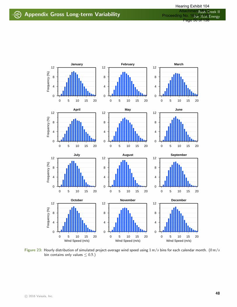
Appendix Gross Long-term VariabilityRush Creek II
For Xcel Energy
. . . . . . . . . . . . . . . . . . . . . . . . . . . . . . . . . . . . . . . . . . . . . . . . . . . . . . . . . . . . . . . . . . . . . . . . . . . . . . . . . . . . . . . . . . . . . . . . . . . . . . . . . . . . . . . . . .
January
0 5 10 15 20
0
4
8
12
Fre
quen
cy (
%)
February
0 5 10 15 20
0
4
8
12March
0 5 10 15 20
0
4
8
12
April
0 5 10 15 20
0
4
8
12
Fre
quen
cy (
%)
May
0 5 10 15 20
0
4
8
12June
0 5 10 15 20
0
4
8
12
July
0 5 10 15 20
0
4
8
12
Fre
quen
cy (
%)
August
0 5 10 15 20
0
4
8
12September
0 5 10 15 20
0
4
8
12
October
0 5 10 15 20Wind Speed (m/s)
0
4
8
12
Fre
quen
cy (
%)
November
0 5 10 15 20Wind Speed (m/s)
0
4
8
12December
0 5 10 15 20Wind Speed (m/s)
0
4
8
12
Figure 23: Hourly distribution of simulated project-average wind speed using 1 m/s bins for each calendar month. (0 m/sbin contains only values ≤ 0.5.)
c© 2016 Vaisala, Inc.48
Hearing Exhibit 104 Attachment MH-2
Proceeding No. 16A-0117E Page 50 of 138
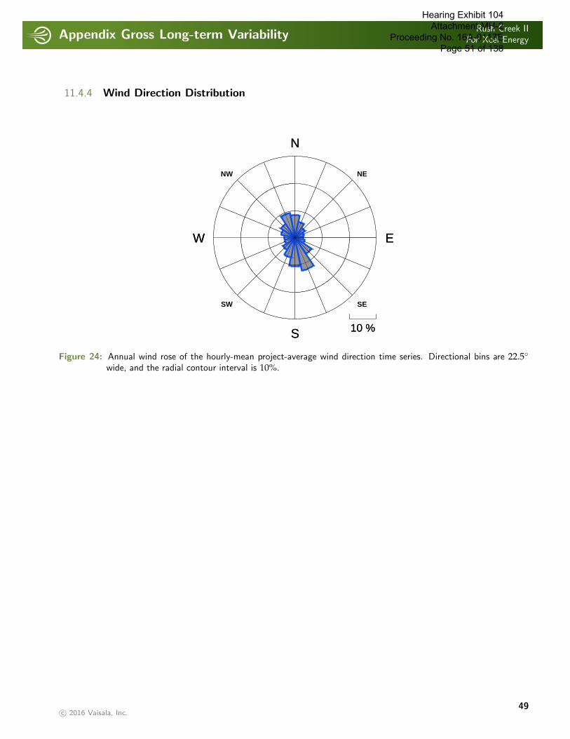
Appendix Gross Long-term VariabilityRush Creek II
For Xcel Energy
. . . . . . . . . . . . . . . . . . . . . . . . . . . . . . . . . . . . . . . . . . . . . . . . . . . . . . . . . . . . . . . . . . . . . . . . . . . . . . . . . . . . . . . . . . . . . . . . . . . . . . . . . . . . . . . . . .
11.4.4 Wind Direction Distribution
S 10 %
EW
N
S 10 %
EW
N
SW
NW
SE
NE
Figure 24: Annual wind rose of the hourly-mean project-average wind direction time series. Directional bins are 22.5◦
wide, and the radial contour interval is 10%.
c© 2016 Vaisala, Inc.49
Hearing Exhibit 104 Attachment MH-2
Proceeding No. 16A-0117E Page 51 of 138

Appendix Gross Long-term VariabilityRush Creek II
For Xcel Energy
. . . . . . . . . . . . . . . . . . . . . . . . . . . . . . . . . . . . . . . . . . . . . . . . . . . . . . . . . . . . . . . . . . . . . . . . . . . . . . . . . . . . . . . . . . . . . . . . . . . . . . . . . . . . . . . . . .
S 10 %
EW
NOctober
S 10 %
EW
N
S 10 %
EW
NNovember
S 10 %
EW
N
S 10 %
EW
NDecember
S 10 %
EW
N
S 10 %
EW
NJuly
S 10 %
EW
N
S 10 %
EW
NAugust
S 10 %
EW
N
S 10 %
EW
NSeptember
S 10 %
EW
N
S 10 %
EW
NApril
S 10 %
EW
N
S 10 %
EW
NMay
S 10 %
EW
N
S 10 %
EW
NJune
S 10 %
EW
N
S 10 %
EW
NJanuary
S 10 %
EW
N
S 10 %
EW
NFebruary
S 10 %
EW
N
S 10 %
EW
NMarch
S 10 %
EW
N
Figure 25: Wind roses of the hourly-mean project-average wind direction time series for each calendar month. Directionalbins are 22.5◦ wide, and the radial contour interval is 10%.
c© 2016 Vaisala, Inc.50
Hearing Exhibit 104 Attachment MH-2
Proceeding No. 16A-0117E Page 52 of 138
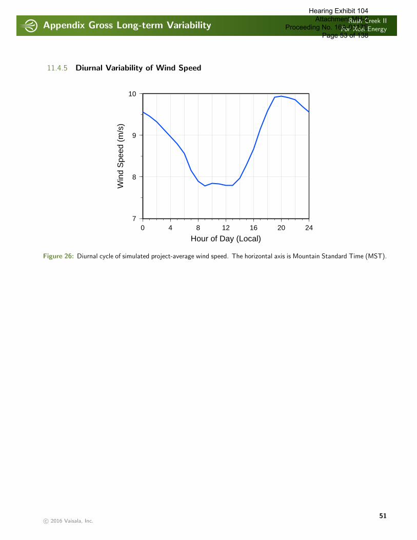
Appendix Gross Long-term VariabilityRush Creek II
For Xcel Energy
. . . . . . . . . . . . . . . . . . . . . . . . . . . . . . . . . . . . . . . . . . . . . . . . . . . . . . . . . . . . . . . . . . . . . . . . . . . . . . . . . . . . . . . . . . . . . . . . . . . . . . . . . . . . . . . . . .
11.4.5 Diurnal Variability of Wind Speed
0 4 8 12 16 20 24
Hour of Day (Local)
7
8
9
10
Win
d S
peed
(m
/s)
Figure 26: Diurnal cycle of simulated project-average wind speed. The horizontal axis is Mountain Standard Time (MST).
c© 2016 Vaisala, Inc.51
Hearing Exhibit 104 Attachment MH-2
Proceeding No. 16A-0117E Page 53 of 138
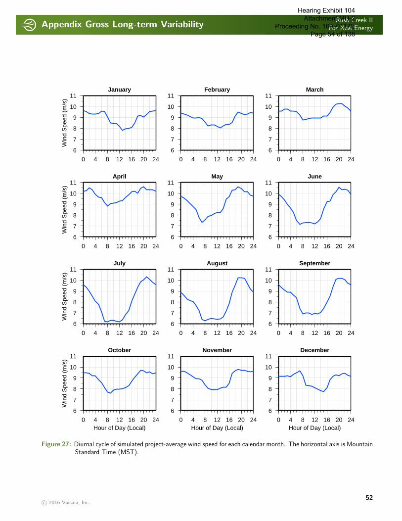
Appendix Gross Long-term VariabilityRush Creek II
For Xcel Energy
. . . . . . . . . . . . . . . . . . . . . . . . . . . . . . . . . . . . . . . . . . . . . . . . . . . . . . . . . . . . . . . . . . . . . . . . . . . . . . . . . . . . . . . . . . . . . . . . . . . . . . . . . . . . . . . . . .
January
0 4 8 12 16 20 24
6
7
8
9
10
11
Win
d S
peed
(m
/s)
February
0 4 8 12 16 20 24
6
7
8
9
10
11March
0 4 8 12 16 20 24
6
7
8
9
10
11
April
0 4 8 12 16 20 24
6
7
8
9
10
11
Win
d S
peed
(m
/s)
May
0 4 8 12 16 20 24
6
7
8
9
10
11June
0 4 8 12 16 20 24
6
7
8
9
10
11
July
0 4 8 12 16 20 24
6
7
8
9
10
11
Win
d S
peed
(m
/s)
August
0 4 8 12 16 20 24
6
7
8
9
10
11September
0 4 8 12 16 20 24
6
7
8
9
10
11
October
0 4 8 12 16 20 24Hour of Day (Local)
6
7
8
9
10
11
Win
d S
peed
(m
/s)
November
0 4 8 12 16 20 24Hour of Day (Local)
6
7
8
9
10
11December
0 4 8 12 16 20 24Hour of Day (Local)
6
7
8
9
10
11
Figure 27: Diurnal cycle of simulated project-average wind speed for each calendar month. The horizontal axis is MountainStandard Time (MST).
c© 2016 Vaisala, Inc.52
Hearing Exhibit 104 Attachment MH-2
Proceeding No. 16A-0117E Page 54 of 138
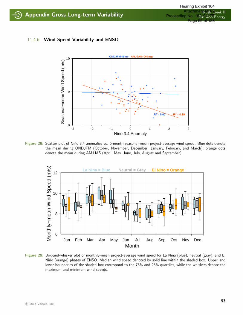
Appendix Gross Long-term VariabilityRush Creek II
For Xcel Energy
. . . . . . . . . . . . . . . . . . . . . . . . . . . . . . . . . . . . . . . . . . . . . . . . . . . . . . . . . . . . . . . . . . . . . . . . . . . . . . . . . . . . . . . . . . . . . . . . . . . . . . . . . . . . . . . . . .
11.4.6 Wind Speed Variability and ENSO
−3 −2 −1 0 1 2 3
Nino 3.4 Anomaly
8
9
10S
easo
nal−
mea
n W
ind
Spe
ed (
m/s
)
R2 = 0.00 R2 = 0.19
ONDJFM=Blue AMJJAS=Orange
Figure 28: Scatter plot of Nino 3.4 anomalies vs. 6-month seasonal-mean project-average wind speed. Blue dots denotethe mean during ONDJFM (October, November, December, January, February, and March); orange dotsdenote the mean during AMJJAS (April, May, June, July, August and September).
Jan Feb Mar Apr May Jun Jul Aug Sep Oct Nov Dec
Month
6
8
10
12
Mon
thly
−m
ean
Win
d S
peed
(m
/s)
La Nina = Blue Neutral = Gray El Nino = Orange
Figure 29: Box-and-whisker plot of monthly-mean project-average wind speed for La Nina (blue), neutral (gray), and ElNino (orange) phases of ENSO. Median wind speed denoted by solid line within the shaded box. Upper andlower boundaries of the shaded box correspond to the 75% and 25% quartiles, while the whiskers denote themaximum and minimum wind speeds.
c© 2016 Vaisala, Inc.53
Hearing Exhibit 104 Attachment MH-2
Proceeding No. 16A-0117E Page 55 of 138
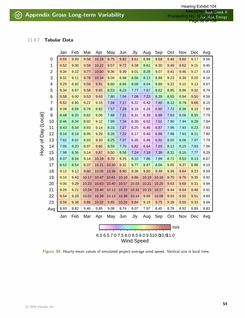
Appendix Gross Long-term VariabilityRush Creek II
For Xcel Energy
. . . . . . . . . . . . . . . . . . . . . . . . . . . . . . . . . . . . . . . . . . . . . . . . . . . . . . . . . . . . . . . . . . . . . . . . . . . . . . . . . . . . . . . . . . . . . . . . . . . . . . . . . . . . . . . . . .
11.4.7 Tabular DataH
our
of D
ay (
Loca
l)
012
34
567
89101112
1314
151617
1819202122
23
Avg
Jan
Jan
Feb
Feb
Mar
Mar
Apr
Apr
May
May
Jun
Jun
Jly
Jly
Aug
Aug
Sep
Sep
Oct
Oct
Nov
Nov
Dec
Dec
Avg
Avg
8.52
9.12
9.16
9.06
9.26
9.54
9.59
9.65
9.52
9.34
9.31
9.29
9.34
9.58
9.52
9.06
8.48
8.46
8.43
8.16
7.82
7.95
7.98
8.07
8.93
8.54
9.12
9.43
9.29
9.21
9.28
9.38
9.39
9.30
9.22
9.11
8.92
8.97
9.00
8.90
8.59
8.20
8.34
8.34
8.18
8.02
8.20
8.36
8.34
8.82
9.37
9.90
10.17
10.23
10.24
10.02
9.86
9.58
9.58
9.77
9.78
9.56
9.58
9.53
9.22
8.78
8.82
8.92
8.93
8.95
8.93
8.97
9.14
9.14
9.46
10.21
10.05
10.47
10.63
10.40
10.39
10.32
10.18
10.22
10.50
10.34
9.91
9.65
9.63
9.15
8.82
9.06
9.12
9.14
9.29
9.33
9.60
9.87
10.18
9.85
10.30
10.36
10.61
10.40
10.13
10.13
9.85
9.75
9.57
9.36
9.09
8.80
8.53
7.80
7.34
7.57
7.88
7.99
8.16
8.26
8.25
8.59
9.50
9.70
9.08
9.32
9.90
10.18
10.57
10.33
10.38
10.26
9.92
9.72
9.39
8.98
8.66
8.23
7.54
7.17
7.28
7.31
7.34
7.27
7.22
7.37
7.70
8.56
9.25
8.74
8.77
9.36
9.86
10.03
10.31
10.14
9.84
9.61
9.38
9.01
8.56
8.08
7.77
7.08
6.22
6.18
6.31
6.30
6.25
6.17
6.35
6.82
7.24
8.10
8.07
8.87
9.50
10.19
10.21
10.15
9.65
9.19
8.89
8.61
8.28
8.13
8.04
7.67
7.23
6.42
6.26
6.39
6.52
6.46
6.40
6.46
6.64
7.18
7.86
7.97
8.56
9.49
10.16
10.25
10.27
10.08
9.75
9.58
9.30
9.07
8.89
8.89
8.62
8.39
7.40
6.90
6.99
7.01
6.87
6.96
6.92
7.03
7.39
7.99
8.45
9.05
9.36
9.70
9.63
9.44
9.53
9.38
9.46
9.49
9.41
9.23
9.22
8.85
8.55
8.12
7.72
7.63
7.90
7.96
7.98
8.02
8.12
8.31
8.71
8.78
9.37
9.64
9.76
9.68
9.64
9.55
9.50
9.60
9.62
9.46
9.30
9.10
8.96
8.94
8.79
8.38
8.06
7.94
7.93
7.93
8.06
8.15
8.16
8.53
8.92
8.88
9.23
9.35
9.31
9.48
9.51
9.33
9.17
9.15
9.17
9.20
9.13
9.32
9.50
9.66
9.19
8.35
8.28
8.23
8.11
7.97
7.83
7.77
8.13
8.89
9.15
9.59
9.92
9.94
9.91
9.85
9.69
9.56
9.45
9.33
9.16
8.97
8.79
8.56
8.15
7.89
7.79
7.84
7.83
7.80
7.79
7.96
8.29
8.67
8.83
6.0 6.5 7.0 7.5 8.0 8.5 9.0 9.510.010.511.0Wind Speed
m/s
Figure 30: Hourly-mean values of simulated project-average wind speed. Vertical axis is local time.
c© 2016 Vaisala, Inc.54
Hearing Exhibit 104 Attachment MH-2
Proceeding No. 16A-0117E Page 56 of 138
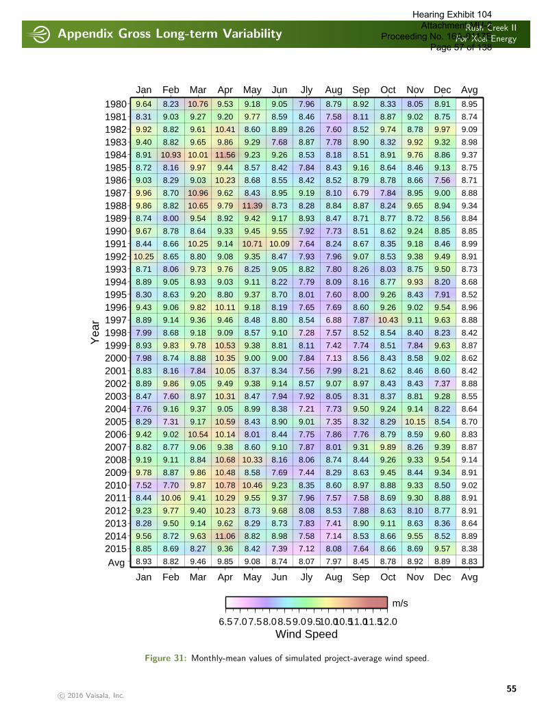
Appendix Gross Long-term VariabilityRush Creek II
For Xcel Energy
. . . . . . . . . . . . . . . . . . . . . . . . . . . . . . . . . . . . . . . . . . . . . . . . . . . . . . . . . . . . . . . . . . . . . . . . . . . . . . . . . . . . . . . . . . . . . . . . . . . . . . . . . . . . . . . . . .
Yea
r198019811982198319841985198619871988198919901991199219931994199519961997199819992000200120022003200420052006200720082009201020112012201320142015Avg
Jan
Jan
Feb
Feb
Mar
Mar
Apr
Apr
May
May
Jun
Jun
Jly
Jly
Aug
Aug
Sep
Sep
Oct
Oct
Nov
Nov
Dec
Dec
Avg
Avg9.64 8.23 10.76 9.53 9.18 9.05 7.96 8.79 8.92 8.33 8.05 8.91
8.31 9.03 9.27 9.20 9.77 8.59 8.46 7.58 8.11 8.87 9.02 8.75
9.92 8.82 9.61 10.41 8.60 8.89 8.26 7.60 8.52 9.74 8.78 9.97
9.40 8.82 9.65 9.86 9.29 7.68 8.87 7.78 8.90 8.32 9.92 9.32
8.91 10.93 10.01 11.56 9.23 9.26 8.53 8.18 8.51 8.91 9.76 8.86
8.72 8.16 9.97 9.44 8.57 8.42 7.84 8.43 9.16 8.64 8.46 9.13
9.03 8.29 9.03 10.23 8.68 8.55 8.42 8.52 8.79 8.78 8.66 7.56
9.96 8.70 10.96 9.62 8.43 8.95 9.19 8.10 6.79 7.84 8.95 9.00
9.86 8.82 10.65 9.79 11.39 8.73 8.28 8.84 8.87 8.24 9.65 8.94
8.74 8.00 9.54 8.92 9.42 9.17 8.93 8.47 8.71 8.77 8.72 8.56
9.67 8.78 8.64 9.33 9.45 9.55 7.92 7.73 8.51 8.62 9.24 8.85
8.44 8.66 10.25 9.14 10.71 10.09 7.64 8.24 8.67 8.35 9.18 8.46
10.25 8.65 8.80 9.08 9.35 8.47 7.93 7.96 9.07 8.53 9.38 9.49
8.71 8.06 9.73 9.76 8.25 9.05 8.82 7.80 8.26 8.03 8.75 9.50
8.89 9.05 8.93 9.03 9.11 8.22 7.79 8.09 8.16 8.77 9.93 8.20
8.30 8.63 9.20 8.80 9.37 8.70 8.01 7.60 8.00 9.26 8.43 7.91
9.43 9.06 9.82 10.11 9.18 8.19 7.65 7.69 8.60 9.26 9.02 9.54
8.89 9.14 9.36 9.46 8.48 8.80 8.54 6.88 7.87 10.43 9.11 9.63
7.99 8.68 9.18 9.09 8.57 9.10 7.28 7.57 8.52 8.54 8.40 8.23
8.93 9.83 9.78 10.53 9.38 8.81 8.11 7.42 7.74 8.51 7.84 9.63
7.98 8.74 8.88 10.35 9.00 9.00 7.84 7.13 8.56 8.43 8.58 9.02
8.83 8.16 7.84 10.05 8.37 8.34 7.56 7.99 8.21 8.62 8.46 8.60
8.89 9.86 9.05 9.49 9.38 9.14 8.57 9.07 8.97 8.43 8.43 7.37
8.47 7.60 8.97 10.31 8.47 7.94 7.92 8.05 8.31 8.37 8.81 9.28
7.76 9.16 9.37 9.05 8.99 8.38 7.21 7.73 9.50 9.24 9.14 8.22
8.29 7.31 9.17 10.59 8.43 8.90 9.01 7.35 8.32 8.29 10.15 8.54
9.42 9.02 10.54 10.14 8.01 8.44 7.75 7.86 7.76 8.79 8.59 9.60
8.82 8.77 9.06 9.38 8.60 9.10 7.87 8.01 9.31 9.89 8.26 9.39
9.19 9.11 8.84 10.68 10.33 8.16 8.06 8.74 8.44 9.26 9.33 9.54
9.78 8.87 9.86 10.48 8.58 7.69 7.44 8.29 8.63 9.45 8.44 9.34
7.52 7.70 9.87 10.78 10.46 9.23 8.35 8.60 8.97 8.88 9.33 8.50
8.44 10.06 9.41 10.29 9.55 9.37 7.96 7.57 7.58 8.69 9.30 8.88
9.23 9.77 9.40 10.23 8.73 9.68 8.08 8.53 7.88 8.63 8.10 8.77
8.28 9.50 9.14 9.62 8.29 8.73 7.83 7.41 8.90 9.11 8.63 8.36
9.56 8.72 9.63 11.06 8.82 8.98 7.58 7.14 8.53 8.66 9.55 8.52
8.85 8.69 8.27 9.36 8.42 7.39 7.12 8.08 7.64 8.66 8.69 9.57
8.93 8.82 9.46 9.85 9.08 8.74 8.07 7.97 8.45 8.78 8.92 8.89
8.95
8.74
9.09
8.98
9.37
8.75
8.71
8.88
9.34
8.84
8.85
8.99
8.91
8.73
8.68
8.52
8.96
8.88
8.42
8.87
8.62
8.42
8.88
8.55
8.64
8.70
8.83
8.87
9.14
8.91
9.02
8.91
8.91
8.64
8.89
8.38
8.83
6.57.07.58.08.59.09.510.010.511.011.512.0Wind Speed
m/s
Figure 31: Monthly-mean values of simulated project-average wind speed.
c© 2016 Vaisala, Inc.55
Hearing Exhibit 104 Attachment MH-2
Proceeding No. 16A-0117E Page 57 of 138
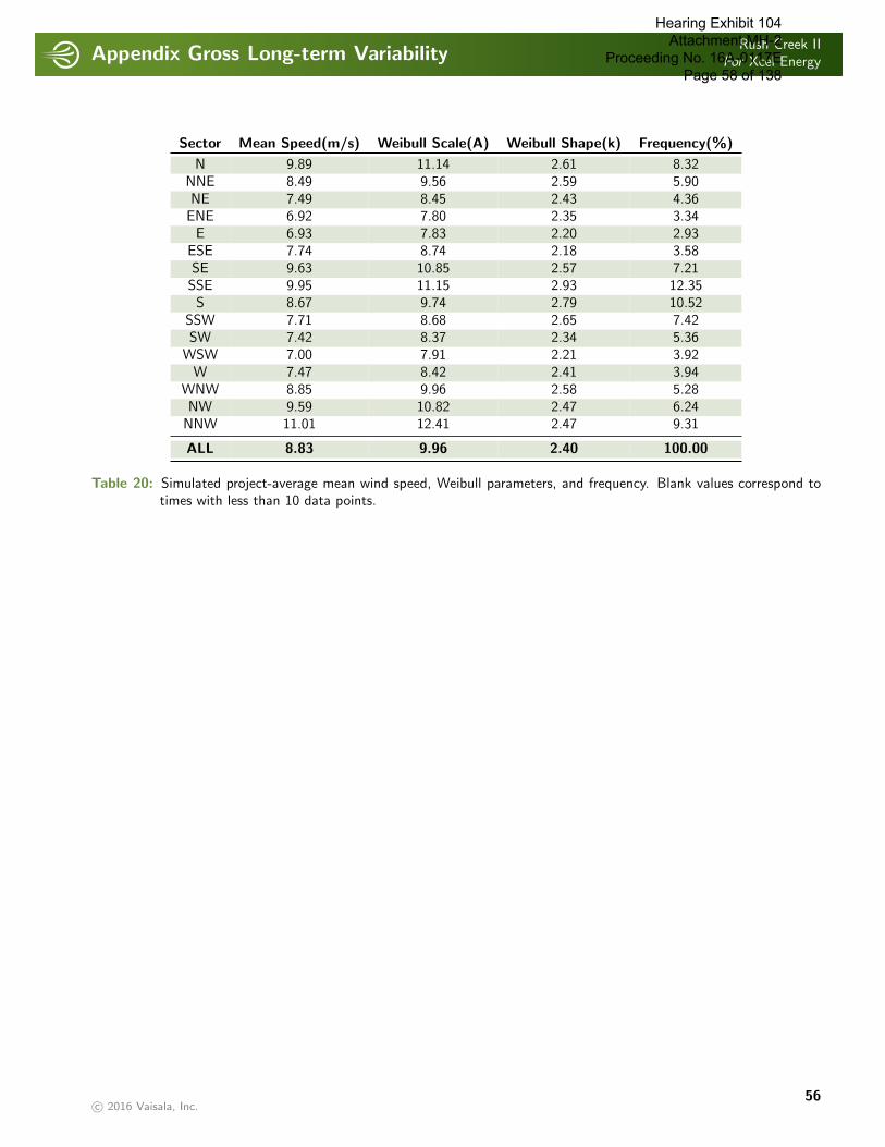
Appendix Gross Long-term VariabilityRush Creek II
For Xcel Energy
. . . . . . . . . . . . . . . . . . . . . . . . . . . . . . . . . . . . . . . . . . . . . . . . . . . . . . . . . . . . . . . . . . . . . . . . . . . . . . . . . . . . . . . . . . . . . . . . . . . . . . . . . . . . . . . . . .
Sector Mean Speed(m/s) Weibull Scale(A) Weibull Shape(k) Frequency(%)
N 9.89 11.14 2.61 8.32NNE 8.49 9.56 2.59 5.90NE 7.49 8.45 2.43 4.36ENE 6.92 7.80 2.35 3.34E 6.93 7.83 2.20 2.93
ESE 7.74 8.74 2.18 3.58SE 9.63 10.85 2.57 7.21SSE 9.95 11.15 2.93 12.35S 8.67 9.74 2.79 10.52
SSW 7.71 8.68 2.65 7.42SW 7.42 8.37 2.34 5.36
WSW 7.00 7.91 2.21 3.92W 7.47 8.42 2.41 3.94
WNW 8.85 9.96 2.58 5.28NW 9.59 10.82 2.47 6.24
NNW 11.01 12.41 2.47 9.31
ALL 8.83 9.96 2.40 100.00
Table 20: Simulated project-average mean wind speed, Weibull parameters, and frequency. Blank values correspond totimes with less than 10 data points.
c© 2016 Vaisala, Inc.56
Hearing Exhibit 104 Attachment MH-2
Proceeding No. 16A-0117E Page 58 of 138

Appendix Gross Long-term VariabilityRush Creek II
For Xcel Energy
. . . . . . . . . . . . . . . . . . . . . . . . . . . . . . . . . . . . . . . . . . . . . . . . . . . . . . . . . . . . . . . . . . . . . . . . . . . . . . . . . . . . . . . . . . . . . . . . . . . . . . . . . . . . . . . . . .
Win
dSpee
dN
NN
EN
EEN
EE
ESE
SE
SSE
SSSW
SW
WSW
WW
NW
NW
NN
WA
ll(m
/s)
0-
0.5
0.00
0.00
0.00
0.00
0.01
0.01
0.00
0.00
0.00
0.00
0.00
0.00
0.00
0.00
0.00
0.00
0.05
0.5
-1.
50.
030.
040.
040.
060.
060.
070.
050.
060.
050.
040.
040.
040.
030.
040.
040.
040.
741.
5-
2.5
0.13
0.13
0.17
0.15
0.17
0.15
0.16
0.14
0.14
0.14
0.14
0.13
0.12
0.13
0.12
0.13
2.26
2.5
-3.
50.
230.
260.
280.
280.
240.
230.
230.
260.
300.
320.
310.
280.
260.
240.
210.
234.
163.
5-
4.5
0.35
0.39
0.36
0.34
0.30
0.30
0.34
0.42
0.51
0.54
0.50
0.42
0.34
0.30
0.30
0.31
6.03
4.5
-5.
50.
490.
460.
450.
370.
320.
340.
430.
590.
730.
710.
640.
560.
450.
380.
350.
407.
655.
5-
6.5
0.59
0.54
0.49
0.38
0.31
0.34
0.51
0.76
0.96
0.93
0.71
0.58
0.47
0.41
0.44
0.51
8.93
6.5
-7.
50.
680.
600.
520.
420.
320.
350.
610.
991.
171.
020.
720.
510.
450.
450.
520.
619.
947.
5-
8.5
0.74
0.65
0.51
0.36
0.30
0.34
0.63
1.15
1.34
1.00
0.63
0.38
0.42
0.51
0.58
0.72
10.2
78.
5-
9.5
0.77
0.60
0.40
0.29
0.26
0.31
0.60
1.24
1.35
0.87
0.47
0.27
0.36
0.50
0.62
0.77
9.66
9.5
-10
.50.
760.
570.
340.
240.
210.
280.
611.
271.
170.
650.
370.
190.
300.
560.
590.
808.
9210
.5-
11.5
0.70
0.49
0.28
0.19
0.16
0.26
0.61
1.25
0.95
0.43
0.27
0.15
0.25
0.49
0.59
0.79
7.87
11.5
-12
.50.
660.
400.
210.
120.
120.
200.
591.
170.
660.
290.
170.
120.
180.
430.
500.
766.
5712
.5-
13.5
0.62
0.28
0.13
0.07
0.07
0.13
0.53
0.98
0.41
0.18
0.12
0.09
0.13
0.32
0.39
0.64
5.09
13.5
-14
.50.
450.
190.
080.
030.
040.
100.
440.
800.
300.
110.
090.
070.
070.
220.
270.
563.
8114
.5-
15.5
0.34
0.14
0.05
0.02
0.02
0.06
0.32
0.52
0.19
0.07
0.06
0.05
0.05
0.13
0.21
0.47
2.69
15.5
-16
.50.
280.
080.
030.
010.
010.
040.
220.
300.
100.
050.
040.
030.
020.
080.
150.
371.
8316
.5-
17.5
0.21
0.04
0.01
0.01
0.01
0.02
0.12
0.18
0.05
0.03
0.03
0.02
0.01
0.04
0.10
0.33
1.21
17.5
-18
.50.
110.
020.
010.
000.
000.
010.
080.
100.
050.
020.
020.
020.
010.
020.
070.
240.
7718
.5-
19.5
0.07
0.01
0.01
0.00
0.00
0.01
0.05
0.06
0.03
0.01
0.01
0.01
0.00
0.01
0.04
0.17
0.50
19.5
-20
.50.
050.
010.
000.
000.
000.
010.
030.
040.
010.
010.
010.
010.
000.
010.
040.
120.
3320
.5-
21.5
0.03
0.00
0.00
0.00
0.00
0.00
0.01
0.03
0.01
0.01
0.01
0.00
0.00
0.01
0.02
0.09
0.23
21.5
-22
.50.
020.
000.
000.
000.
000.
000.
010.
010.
010.
000.
010.
000.
000.
010.
020.
070.
1722
.5-
23.5
0.01
0.00
0.00
0.00
0.00
0.00
0.00
0.01
0.01
0.00
0.00
0.00
0.00
0.00
0.01
0.05
0.11
23.5
-24
.50.
010.
000.
000.
000.
000.
000.
000.
010.
000.
000.
000.
000.
000.
000.
010.
040.
08>
24.5
0.00
0.00
0.00
0.00
0.00
0.00
0.00
0.01
0.01
0.00
0.00
0.00
0.00
0.00
0.01
0.08
0.12
Table
21:
Distr
ibution
ofsim
ula
ted
proj
ect-
aver
age
win
dsp
eed
bydirec
tion
.
c© 2016 Vaisala, Inc.57
Hearing Exhibit 104 Attachment MH-2
Proceeding No. 16A-0117E Page 59 of 138
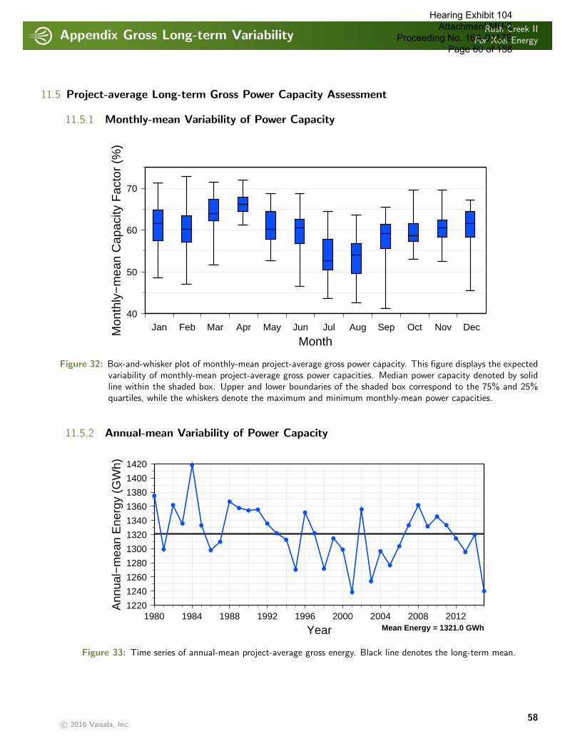
Appendix Gross Long-term VariabilityRush Creek II
For Xcel Energy
. . . . . . . . . . . . . . . . . . . . . . . . . . . . . . . . . . . . . . . . . . . . . . . . . . . . . . . . . . . . . . . . . . . . . . . . . . . . . . . . . . . . . . . . . . . . . . . . . . . . . . . . . . . . . . . . . .
11.5 Project-average Long-term Gross Power Capacity Assessment
11.5.1 Monthly-mean Variability of Power Capacity
Jan Feb Mar Apr May Jun Jul Aug Sep Oct Nov Dec
Month
40
50
60
70
Mon
thly
−m
ean
Cap
acity
Fac
tor
(%)
Figure 32: Box-and-whisker plot of monthly-mean project-average gross power capacity. This figure displays the expectedvariability of monthly-mean project-average gross power capacities. Median power capacity denoted by solidline within the shaded box. Upper and lower boundaries of the shaded box correspond to the 75% and 25%quartiles, while the whiskers denote the maximum and minimum monthly-mean power capacities.
11.5.2 Annual-mean Variability of Power Capacity
1220
1240
1260
1280
1300
1320
1340
1360
1380
1400
1420
Ann
ual−
mea
n E
nerg
y (G
Wh)
1980 1984 1988 1992 1996 2000 2004 2008 2012
Year Mean Energy = 1321.0 GWh
Figure 33: Time series of annual-mean project-average gross energy. Black line denotes the long-term mean.
c© 2016 Vaisala, Inc.58
Hearing Exhibit 104 Attachment MH-2
Proceeding No. 16A-0117E Page 60 of 138
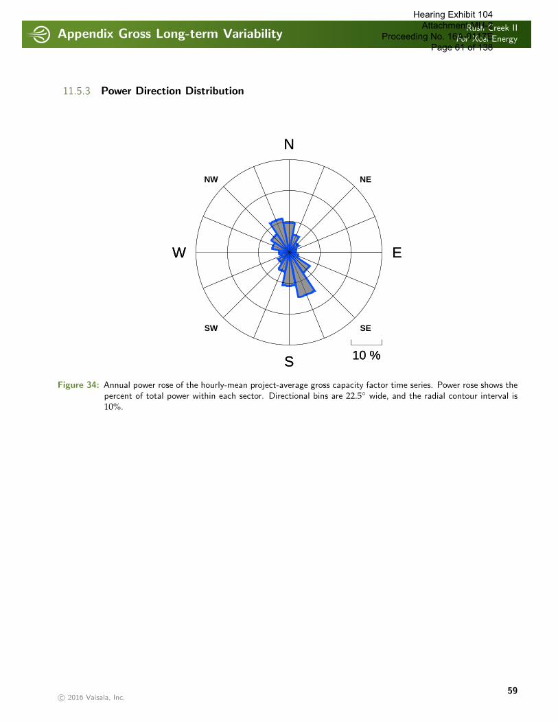
Appendix Gross Long-term VariabilityRush Creek II
For Xcel Energy
. . . . . . . . . . . . . . . . . . . . . . . . . . . . . . . . . . . . . . . . . . . . . . . . . . . . . . . . . . . . . . . . . . . . . . . . . . . . . . . . . . . . . . . . . . . . . . . . . . . . . . . . . . . . . . . . . .
11.5.3 Power Direction Distribution
S 10 %
EW
N
S 10 %
EW
N
SW
NW
SE
NE
Figure 34: Annual power rose of the hourly-mean project-average gross capacity factor time series. Power rose shows thepercent of total power within each sector. Directional bins are 22.5◦ wide, and the radial contour interval is10%.
c© 2016 Vaisala, Inc.59
Hearing Exhibit 104 Attachment MH-2
Proceeding No. 16A-0117E Page 61 of 138
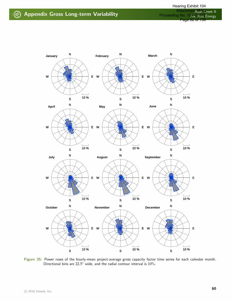
Appendix Gross Long-term VariabilityRush Creek II
For Xcel Energy
. . . . . . . . . . . . . . . . . . . . . . . . . . . . . . . . . . . . . . . . . . . . . . . . . . . . . . . . . . . . . . . . . . . . . . . . . . . . . . . . . . . . . . . . . . . . . . . . . . . . . . . . . . . . . . . . . .
S 10 %
EW
NOctober
S 10 %
EW
N
S 10 %
EW
NNovember
S 10 %
EW
N
S 10 %
EW
NDecember
S 10 %
EW
N
S 10 %
EW
NJuly
S 10 %
EW
N
S 10 %
EW
NAugust
S 10 %
EW
N
S 10 %
EW
NSeptember
S 10 %
EW
N
S 10 %
EW
NApril
S 10 %
EW
N
S 10 %
EW
NMay
S 10 %
EW
N
S 10 %
EW
NJune
S 10 %
EW
N
S 10 %
EW
NJanuary
S 10 %
EW
N
S 10 %
EW
NFebruary
S 10 %
EW
N
S 10 %
EW
NMarch
S 10 %
EW
N
Figure 35: Power roses of the hourly-mean project-average gross capacity factor time series for each calendar month.Directional bins are 22.5◦ wide, and the radial contour interval is 10%.
c© 2016 Vaisala, Inc.60
Hearing Exhibit 104 Attachment MH-2
Proceeding No. 16A-0117E Page 62 of 138
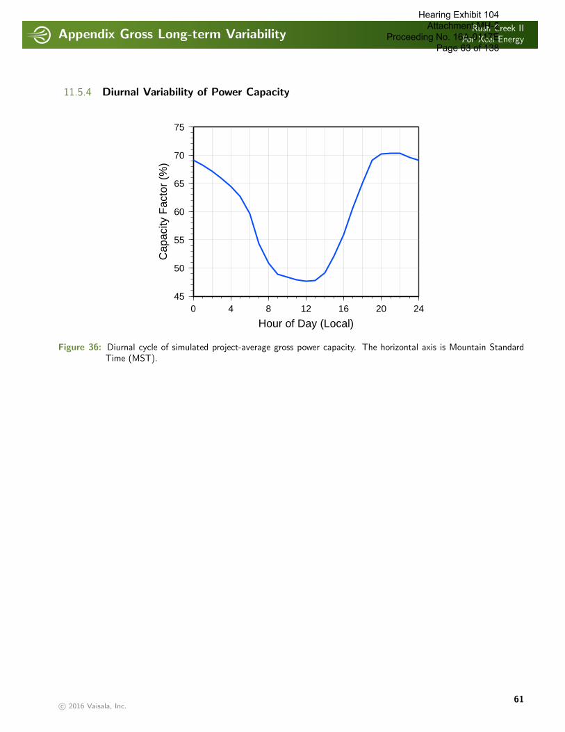
Appendix Gross Long-term VariabilityRush Creek II
For Xcel Energy
. . . . . . . . . . . . . . . . . . . . . . . . . . . . . . . . . . . . . . . . . . . . . . . . . . . . . . . . . . . . . . . . . . . . . . . . . . . . . . . . . . . . . . . . . . . . . . . . . . . . . . . . . . . . . . . . . .
11.5.4 Diurnal Variability of Power Capacity
0 4 8 12 16 20 24
Hour of Day (Local)
45
50
55
60
65
70
75
Cap
acity
Fac
tor
(%)
Figure 36: Diurnal cycle of simulated project-average gross power capacity. The horizontal axis is Mountain StandardTime (MST).
c© 2016 Vaisala, Inc.61
Hearing Exhibit 104 Attachment MH-2
Proceeding No. 16A-0117E Page 63 of 138
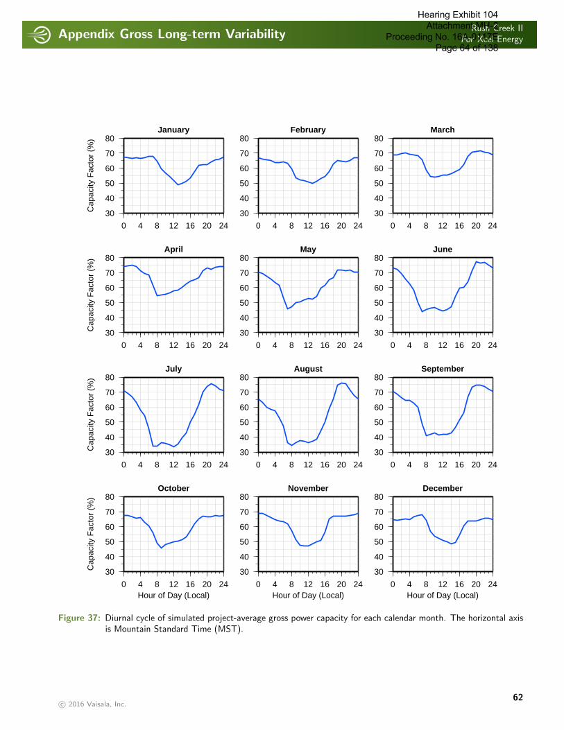
Appendix Gross Long-term VariabilityRush Creek II
For Xcel Energy
. . . . . . . . . . . . . . . . . . . . . . . . . . . . . . . . . . . . . . . . . . . . . . . . . . . . . . . . . . . . . . . . . . . . . . . . . . . . . . . . . . . . . . . . . . . . . . . . . . . . . . . . . . . . . . . . . .
January
0 4 8 12 16 20 24
30
40
50
60
70
80
Cap
acity
Fac
tor
(%)
February
0 4 8 12 16 20 24
30
40
50
60
70
80March
0 4 8 12 16 20 24
30
40
50
60
70
80
April
0 4 8 12 16 20 24
30
40
50
60
70
80
Cap
acity
Fac
tor
(%)
May
0 4 8 12 16 20 24
30
40
50
60
70
80June
0 4 8 12 16 20 24
30
40
50
60
70
80
July
0 4 8 12 16 20 24
30
40
50
60
70
80
Cap
acity
Fac
tor
(%)
August
0 4 8 12 16 20 24
30
40
50
60
70
80September
0 4 8 12 16 20 24
30
40
50
60
70
80
October
0 4 8 12 16 20 24Hour of Day (Local)
30
40
50
60
70
80
Cap
acity
Fac
tor
(%)
November
0 4 8 12 16 20 24Hour of Day (Local)
30
40
50
60
70
80December
0 4 8 12 16 20 24Hour of Day (Local)
30
40
50
60
70
80
Figure 37: Diurnal cycle of simulated project-average gross power capacity for each calendar month. The horizontal axisis Mountain Standard Time (MST).
c© 2016 Vaisala, Inc.62
Hearing Exhibit 104 Attachment MH-2
Proceeding No. 16A-0117E Page 64 of 138
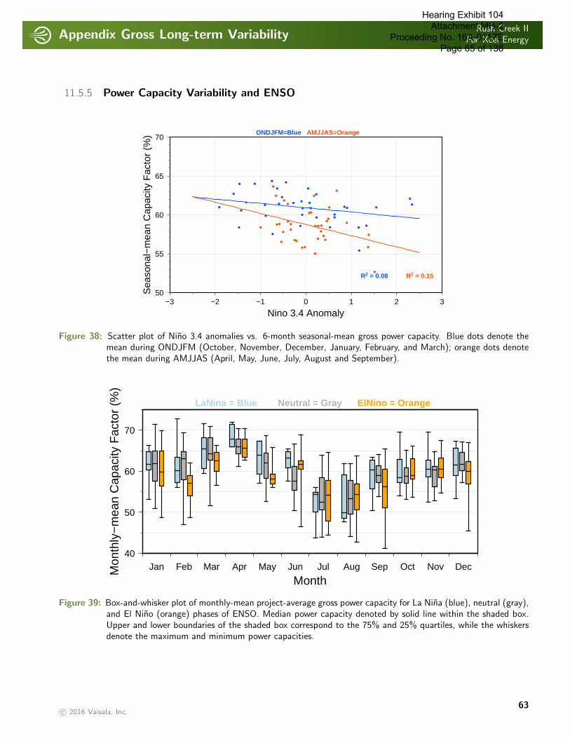
Appendix Gross Long-term VariabilityRush Creek II
For Xcel Energy
. . . . . . . . . . . . . . . . . . . . . . . . . . . . . . . . . . . . . . . . . . . . . . . . . . . . . . . . . . . . . . . . . . . . . . . . . . . . . . . . . . . . . . . . . . . . . . . . . . . . . . . . . . . . . . . . . .
11.5.5 Power Capacity Variability and ENSO
−3 −2 −1 0 1 2 3
Nino 3.4 Anomaly
50
55
60
65
70S
easo
nal−
mea
n C
apac
ity F
acto
r (%
)
R2 = 0.08 R2 = 0.15
ONDJFM=Blue AMJJAS=Orange
Figure 38: Scatter plot of Nino 3.4 anomalies vs. 6-month seasonal-mean gross power capacity. Blue dots denote themean during ONDJFM (October, November, December, January, February, and March); orange dots denotethe mean during AMJJAS (April, May, June, July, August and September).
Jan Feb Mar Apr May Jun Jul Aug Sep Oct Nov Dec
Month
40
50
60
70
Mon
thly
−m
ean
Cap
acity
Fac
tor
(%)
LaNina = Blue Neutral = Gray ElNino = Orange
Figure 39: Box-and-whisker plot of monthly-mean project-average gross power capacity for La Nina (blue), neutral (gray),and El Nino (orange) phases of ENSO. Median power capacity denoted by solid line within the shaded box.Upper and lower boundaries of the shaded box correspond to the 75% and 25% quartiles, while the whiskersdenote the maximum and minimum power capacities.
c© 2016 Vaisala, Inc.63
Hearing Exhibit 104 Attachment MH-2
Proceeding No. 16A-0117E Page 65 of 138
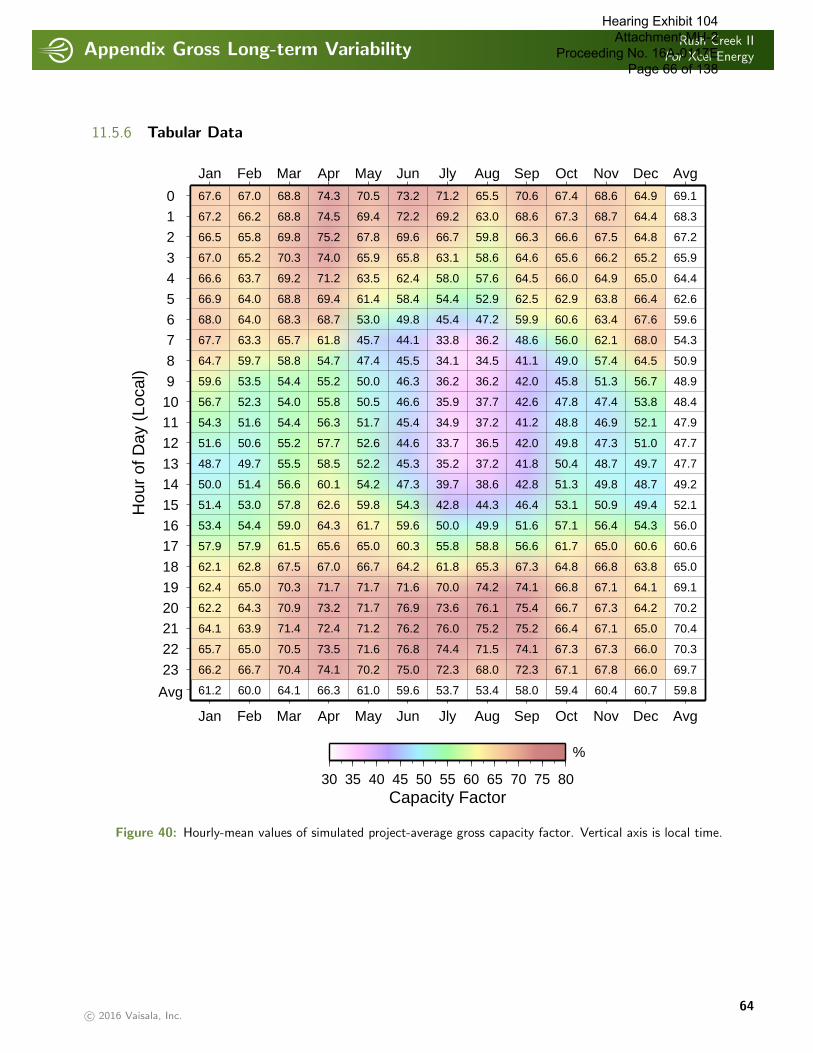
Appendix Gross Long-term VariabilityRush Creek II
For Xcel Energy
. . . . . . . . . . . . . . . . . . . . . . . . . . . . . . . . . . . . . . . . . . . . . . . . . . . . . . . . . . . . . . . . . . . . . . . . . . . . . . . . . . . . . . . . . . . . . . . . . . . . . . . . . . . . . . . . . .
11.5.6 Tabular DataH
our
of D
ay (
Loca
l)
012
34
567
89101112
1314
151617
1819202122
23
Avg
Jan
Jan
Feb
Feb
Mar
Mar
Apr
Apr
May
May
Jun
Jun
Jly
Jly
Aug
Aug
Sep
Sep
Oct
Oct
Nov
Nov
Dec
Dec
Avg
Avg
57.9
62.1
62.4
62.2
64.1
65.7
66.2
67.6
67.2
66.5
67.0
66.6
66.9
68.0
67.7
64.7
59.6
56.7
54.3
51.6
48.7
50.0
51.4
53.4
61.2
57.9
62.8
65.0
64.3
63.9
65.0
66.7
67.0
66.2
65.8
65.2
63.7
64.0
64.0
63.3
59.7
53.5
52.3
51.6
50.6
49.7
51.4
53.0
54.4
60.0
61.5
67.5
70.3
70.9
71.4
70.5
70.4
68.8
68.8
69.8
70.3
69.2
68.8
68.3
65.7
58.8
54.4
54.0
54.4
55.2
55.5
56.6
57.8
59.0
64.1
65.6
67.0
71.7
73.2
72.4
73.5
74.1
74.3
74.5
75.2
74.0
71.2
69.4
68.7
61.8
54.7
55.2
55.8
56.3
57.7
58.5
60.1
62.6
64.3
66.3
65.0
66.7
71.7
71.7
71.2
71.6
70.2
70.5
69.4
67.8
65.9
63.5
61.4
53.0
45.7
47.4
50.0
50.5
51.7
52.6
52.2
54.2
59.8
61.7
61.0
60.3
64.2
71.6
76.9
76.2
76.8
75.0
73.2
72.2
69.6
65.8
62.4
58.4
49.8
44.1
45.5
46.3
46.6
45.4
44.6
45.3
47.3
54.3
59.6
59.6
55.8
61.8
70.0
73.6
76.0
74.4
72.3
71.2
69.2
66.7
63.1
58.0
54.4
45.4
33.8
34.1
36.2
35.9
34.9
33.7
35.2
39.7
42.8
50.0
53.7
58.8
65.3
74.2
76.1
75.2
71.5
68.0
65.5
63.0
59.8
58.6
57.6
52.9
47.2
36.2
34.5
36.2
37.7
37.2
36.5
37.2
38.6
44.3
49.9
53.4
56.6
67.3
74.1
75.4
75.2
74.1
72.3
70.6
68.6
66.3
64.6
64.5
62.5
59.9
48.6
41.1
42.0
42.6
41.2
42.0
41.8
42.8
46.4
51.6
58.0
61.7
64.8
66.8
66.7
66.4
67.3
67.1
67.4
67.3
66.6
65.6
66.0
62.9
60.6
56.0
49.0
45.8
47.8
48.8
49.8
50.4
51.3
53.1
57.1
59.4
65.0
66.8
67.1
67.3
67.1
67.3
67.8
68.6
68.7
67.5
66.2
64.9
63.8
63.4
62.1
57.4
51.3
47.4
46.9
47.3
48.7
49.8
50.9
56.4
60.4
60.6
63.8
64.1
64.2
65.0
66.0
66.0
64.9
64.4
64.8
65.2
65.0
66.4
67.6
68.0
64.5
56.7
53.8
52.1
51.0
49.7
48.7
49.4
54.3
60.7
60.6
65.0
69.1
70.2
70.4
70.3
69.7
69.1
68.3
67.2
65.9
64.4
62.6
59.6
54.3
50.9
48.9
48.4
47.9
47.7
47.7
49.2
52.1
56.0
59.8
30 35 40 45 50 55 60 65 70 75 80Capacity Factor
%
Figure 40: Hourly-mean values of simulated project-average gross capacity factor. Vertical axis is local time.
c© 2016 Vaisala, Inc.64
Hearing Exhibit 104 Attachment MH-2
Proceeding No. 16A-0117E Page 66 of 138
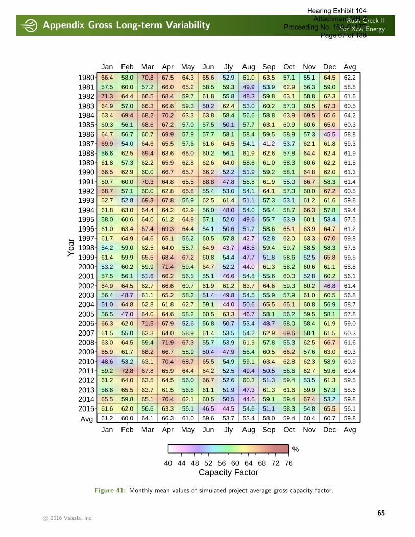
Appendix Gross Long-term VariabilityRush Creek II
For Xcel Energy
. . . . . . . . . . . . . . . . . . . . . . . . . . . . . . . . . . . . . . . . . . . . . . . . . . . . . . . . . . . . . . . . . . . . . . . . . . . . . . . . . . . . . . . . . . . . . . . . . . . . . . . . . . . . . . . . . .
Yea
r198019811982198319841985198619871988198919901991199219931994199519961997199819992000200120022003200420052006200720082009201020112012201320142015Avg
Jan
Jan
Feb
Feb
Mar
Mar
Apr
Apr
May
May
Jun
Jun
Jly
Jly
Aug
Aug
Sep
Sep
Oct
Oct
Nov
Nov
Dec
Dec
Avg
Avg66.4 58.0 70.8 67.5 64.3 65.6 52.9 61.0 63.5 57.1 55.1 64.5
57.5 60.0 57.2 66.0 65.2 58.5 59.3 49.9 53.9 62.9 56.3 59.0
71.3 64.4 66.5 68.4 59.7 61.8 55.8 48.3 59.8 63.1 58.8 62.3
64.9 57.0 66.3 66.6 59.3 50.2 62.4 53.0 60.2 57.3 60.5 67.3
63.4 69.4 68.2 70.2 63.3 63.8 58.4 56.6 58.8 63.9 69.5 65.6
60.3 56.1 68.6 67.2 57.0 57.5 50.1 57.7 63.1 60.9 60.6 65.0
64.7 56.7 60.7 69.9 57.9 57.7 58.1 58.4 59.5 58.9 57.3 45.5
69.9 54.0 64.6 65.5 57.6 61.6 64.5 54.1 41.2 53.7 62.1 61.8
56.6 62.5 69.4 63.6 65.0 60.2 56.1 61.9 62.6 57.8 64.4 62.4
61.8 57.3 62.2 65.9 62.8 62.6 64.0 58.6 61.0 58.3 60.6 62.2
66.5 62.9 60.0 66.7 65.7 66.2 52.2 51.9 59.2 58.1 64.8 62.0
60.7 60.0 70.3 64.8 65.5 68.8 47.8 56.8 61.9 55.0 66.7 58.3
68.7 57.1 60.0 62.8 65.8 55.4 53.0 54.1 64.1 57.3 60.0 67.2
62.7 52.8 69.3 67.8 56.9 62.5 61.4 51.1 57.3 53.1 61.2 61.6
61.8 63.0 64.4 64.2 62.9 56.0 48.0 54.0 56.4 58.7 66.3 57.8
58.0 60.6 64.0 61.2 64.9 57.1 52.0 49.6 55.7 53.9 60.1 53.4
61.0 63.4 67.4 69.3 64.4 54.1 50.6 51.7 58.6 65.1 63.9 64.7
61.7 64.9 64.6 65.1 56.2 60.5 57.8 42.7 52.8 62.0 63.3 67.0
54.2 59.0 62.5 64.0 58.7 64.9 43.7 48.5 59.4 59.7 58.5 58.3
61.4 59.9 65.5 68.4 67.2 60.8 54.4 47.7 51.8 58.6 52.5 65.8
53.2 60.2 59.9 71.4 59.4 64.7 52.2 44.0 61.3 58.2 60.6 61.1
57.5 56.1 51.6 66.2 56.5 55.1 46.6 54.8 55.6 60.0 52.8 60.2
64.9 64.5 62.7 66.6 60.7 61.9 61.2 63.7 64.6 59.3 60.2 46.8
56.4 48.7 61.1 65.2 58.2 51.4 49.8 54.5 55.9 57.9 61.0 60.5
51.0 64.8 62.8 61.8 62.7 59.1 44.0 50.6 65.5 65.1 60.8 56.9
56.5 47.0 64.0 64.6 58.2 60.5 63.3 46.7 58.1 56.2 59.5 58.1
66.3 62.0 71.5 67.9 52.6 56.8 50.7 53.4 48.7 58.0 58.4 61.9
61.5 55.0 63.3 64.0 58.9 61.4 53.5 54.2 62.9 69.6 58.1 61.5
63.0 64.5 59.4 71.9 67.3 55.7 53.9 61.9 57.8 55.3 62.5 66.7
65.9 61.7 68.2 66.7 58.9 50.4 47.9 56.4 60.5 66.2 57.6 63.0
48.6 53.2 63.1 70.4 68.7 65.5 54.9 59.1 63.4 62.8 62.3 58.9
59.2 72.8 67.8 65.9 64.4 64.2 52.5 49.4 50.5 56.6 62.7 59.6
61.2 64.0 63.5 64.5 56.0 66.7 52.6 60.3 51.3 59.4 53.5 61.3
56.6 65.5 63.7 61.5 56.8 61.1 51.9 47.3 61.3 61.6 59.9 57.3
65.5 59.8 65.1 70.4 62.1 60.5 50.5 44.6 59.1 59.4 67.4 53.2
61.6 62.0 56.6 63.3 56.1 46.5 44.5 54.6 51.1 58.3 54.8 65.5
61.2 60.0 64.1 66.3 61.0 59.6 53.7 53.4 58.0 59.4 60.4 60.7
62.2
58.8
61.6
60.5
64.2
60.3
58.8
59.3
61.9
61.5
61.3
61.4
60.5
59.8
59.4
57.5
61.2
59.8
57.6
59.5
58.8
56.1
61.4
56.8
58.7
57.8
59.0
60.3
61.6
60.3
60.9
60.4
59.5
58.6
59.8
56.1
59.8
40 44 48 52 56 60 64 68 72 76Capacity Factor
%
Figure 41: Monthly-mean values of simulated project-average gross capacity factor.
c© 2016 Vaisala, Inc.65
Hearing Exhibit 104 Attachment MH-2
Proceeding No. 16A-0117E Page 67 of 138
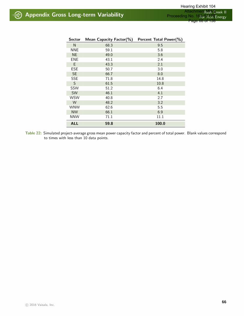
Appendix Gross Long-term VariabilityRush Creek II
For Xcel Energy
. . . . . . . . . . . . . . . . . . . . . . . . . . . . . . . . . . . . . . . . . . . . . . . . . . . . . . . . . . . . . . . . . . . . . . . . . . . . . . . . . . . . . . . . . . . . . . . . . . . . . . . . . . . . . . . . . .
Sector Mean Capacity Factor(%) Percent Total Power(%)
N 68.3 9.5NNE 59.1 5.8NE 49.0 3.6ENE 43.1 2.4E 43.3 2.1
ESE 50.7 3.0SE 66.7 8.0SSE 71.8 14.8S 61.5 10.8
SSW 51.2 6.4SW 46.1 4.1
WSW 40.8 2.7W 48.2 3.2
WNW 62.6 5.5NW 66.1 6.9
NNW 71.1 11.1
ALL 59.8 100.0
Table 22: Simulated project-average gross mean power capacity factor and percent of total power. Blank values correspondto times with less than 10 data points.
c© 2016 Vaisala, Inc.66
Hearing Exhibit 104 Attachment MH-2
Proceeding No. 16A-0117E Page 68 of 138
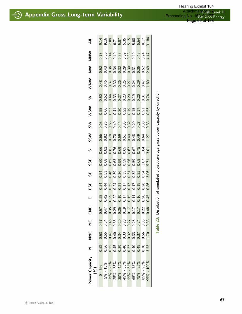
Appendix Gross Long-term VariabilityRush Creek II
For Xcel Energy
. . . . . . . . . . . . . . . . . . . . . . . . . . . . . . . . . . . . . . . . . . . . . . . . . . . . . . . . . . . . . . . . . . . . . . . . . . . . . . . . . . . . . . . . . . . . . . . . . . . . . . . . . . . . . . . . . .
Power
Capaci
tyN
NN
EN
EEN
EE
ESE
SE
SSE
SSSW
SW
WSW
WW
NW
NW
NN
WA
ll(%
)
0-
5%0.
520.
530.
570.
570.
550.
540.
540.
600.
660.
660.
630.
550.
500.
480.
520.
739.
145%
-15
%0.
560.
550.
540.
470.
420.
440.
530.
680.
820.
820.
750.
660.
520.
460.
430.
509.
1615
%-
25%
0.52
0.47
0.45
0.35
0.29
0.32
0.46
0.65
0.81
0.78
0.63
0.53
0.44
0.37
0.36
0.44
7.89
25%
-35
%0.
450.
400.
350.
290.
220.
240.
390.
630.
760.
700.
490.
410.
330.
300.
340.
406.
7135
%-
45%
0.39
0.34
0.29
0.26
0.19
0.21
0.36
0.59
0.69
0.59
0.44
0.30
0.27
0.26
0.32
0.38
5.87
45%
-55
%0.
400.
330.
280.
190.
170.
170.
350.
590.
650.
510.
330.
220.
230.
250.
290.
395.
3555
%-
65%
0.37
0.32
0.27
0.17
0.15
0.17
0.31
0.56
0.67
0.49
0.32
0.19
0.20
0.27
0.30
0.38
5.15
65%
-75
%0.
400.
330.
230.
170.
140.
170.
320.
590.
670.
480.
290.
150.
190.
240.
310.
405.
0875
%-
85%
0.48
0.37
0.24
0.17
0.16
0.18
0.35
0.68
0.75
0.49
0.27
0.17
0.20
0.29
0.35
0.48
5.64
85%
-95
%0.
700.
560.
330.
220.
200.
260.
541.
071.
040.
640.
380.
210.
310.
470.
520.
748.
1795
%-10
0%3.
531.
700.
830.
480.
450.
863.
065.
713.
011.
270.
830.
530.
741.
892.
494.
4731
.84
Tabl e
23:
Distr
ibution
ofsim
ula
ted
proj
ect-
aver
age
gros
spow
erca
pac
ity
bydirec
tion
.
c© 2016 Vaisala, Inc.67
Hearing Exhibit 104 Attachment MH-2
Proceeding No. 16A-0117E Page 69 of 138

Appendix Gross Long-term VariabilityRush Creek II
For Xcel Energy
. . . . . . . . . . . . . . . . . . . . . . . . . . . . . . . . . . . . . . . . . . . . . . . . . . . . . . . . . . . . . . . . . . . . . . . . . . . . . . . . . . . . . . . . . . . . . . . . . . . . . . . . . . . . . . . . . .
11.6 Long-term Wind Resource Assessment for Tower M2196 at 80 m
11.6.1 Tabular Data
Sector Mean Speed(m/s) Weibull Scale(A) Weibull Shape(k) Frequency(%)
N 9.91 11.17 2.47 8.74NNE 8.33 9.39 2.47 5.92NE 7.51 8.47 2.41 4.54ENE 6.85 7.73 2.39 3.53E 6.77 7.64 2.24 2.93
ESE 7.44 8.40 2.05 3.14SE 9.61 10.84 2.30 5.81SSE 10.52 11.81 2.79 11.59S 9.14 10.27 2.76 11.58
SSW 7.87 8.86 2.64 8.44SW 7.19 8.12 2.26 5.95
WSW 6.65 7.51 2.20 4.20W 7.19 8.11 2.36 4.19
WNW 8.56 9.65 2.44 5.18NW 9.31 10.50 2.31 5.67
NNW 10.83 12.22 2.36 8.59
ALL 8.78 9.91 2.29 100.00
Table 24: Simulated mean wind speed, Weibull parameters, and frequency for Tower M2196 at 80 m. Blank valuescorrespond to times with less than 10 data points.
c© 2016 Vaisala, Inc.68
Hearing Exhibit 104 Attachment MH-2
Proceeding No. 16A-0117E Page 70 of 138

Appendix Gross Long-term VariabilityRush Creek II
For Xcel Energy
. . . . . . . . . . . . . . . . . . . . . . . . . . . . . . . . . . . . . . . . . . . . . . . . . . . . . . . . . . . . . . . . . . . . . . . . . . . . . . . . . . . . . . . . . . . . . . . . . . . . . . . . . . . . . . . . . .
Win
dSpee
dN
NN
EN
EEN
EE
ESE
SE
SSE
SSSW
SW
WSW
WW
NW
NW
NN
WA
ll(m
/s)
0-
0.5
0.02
0.02
0.01
0.02
0.02
0.03
0.04
0.05
0.03
0.02
0.01
0.02
0.02
0.03
0.02
0.03
0.40
0.5
-1.
50.
070.
060.
050.
060.
060.
070.
080.
060.
070.
060.
050.
050.
050.
050.
060.
060.
941.
5-
2.5
0.14
0.14
0.16
0.13
0.14
0.15
0.14
0.14
0.16
0.16
0.15
0.13
0.14
0.13
0.14
0.13
2.29
2.5
-3.
50.
260.
300.
280.
270.
250.
250.
220.
240.
300.
350.
390.
310.
290.
240.
210.
234.
363.
5-
4.5
0.41
0.42
0.39
0.38
0.33
0.30
0.29
0.38
0.49
0.60
0.62
0.54
0.41
0.33
0.29
0.32
6.49
4.5
-5.
50.
460.
440.
430.
380.
330.
280.
320.
460.
650.
730.
730.
620.
470.
350.
340.
367.
365.
5-
6.5
0.60
0.54
0.47
0.43
0.33
0.29
0.42
0.60
0.87
0.96
0.83
0.65
0.49
0.43
0.40
0.48
8.77
6.5
-7.
50.
720.
640.
570.
450.
340.
300.
470.
831.
181.
140.
840.
580.
530.
490.
540.
6010
.22
7.5
-8.
50.
770.
630.
500.
390.
310.
300.
490.
931.
331.
080.
630.
380.
460.
520.
520.
699.
928.
5-
9.5
0.77
0.59
0.44
0.31
0.25
0.25
0.46
1.00
1.34
0.97
0.47
0.25
0.40
0.52
0.54
0.70
9.27
9.5
-10
.50.
830.
580.
390.
280.
210.
250.
481.
121.
350.
850.
370.
210.
320.
570.
540.
819.
1710
.5-
11.5
0.73
0.45
0.29
0.17
0.15
0.22
0.43
1.03
1.11
0.55
0.26
0.14
0.23
0.46
0.48
0.68
7.37
11.5
-12
.50.
670.
380.
210.
130.
100.
160.
441.
070.
920.
370.
180.
110.
150.
400.
430.
666.
3812
.5-
13.5
0.57
0.25
0.13
0.06
0.05
0.10
0.38
0.94
0.60
0.23
0.12
0.07
0.09
0.25
0.31
0.52
4.66
13.5
-14
.50.
440.
180.
080.
030.
030.
070.
290.
790.
390.
130.
080.
050.
050.
150.
210.
413.
4014
.5-
15.5
0.35
0.13
0.06
0.02
0.02
0.05
0.24
0.65
0.30
0.07
0.05
0.03
0.03
0.10
0.17
0.40
2.67
15.5
-16
.50.
310.
100.
030.
010.
010.
030.
230.
530.
210.
060.
050.
030.
020.
070.
150.
372.
1916
.5-
17.5
0.23
0.05
0.02
0.00
0.01
0.02
0.16
0.35
0.11
0.04
0.04
0.02
0.01
0.04
0.11
0.33
1.54
17.5
-18
.50.
150.
020.
010.
000.
000.
010.
090.
180.
060.
020.
020.
010.
010.
020.
060.
220.
9018
.5-
19.5
0.08
0.01
0.00
0.00
0.00
0.01
0.05
0.09
0.04
0.01
0.01
0.01
0.00
0.01
0.04
0.15
0.51
19.5
-20
.50.
070.
010.
000.
000.
000.
000.
040.
080.
030.
010.
010.
010.
000.
010.
030.
140.
4520
.5-
21.5
0.03
0.00
0.00
0.00
0.00
0.00
0.02
0.03
0.01
0.01
0.01
0.00
0.00
0.01
0.02
0.08
0.22
21.5
-22
.50.
030.
000.
000.
000.
000.
000.
010.
030.
010.
000.
010.
000.
000.
010.
020.
070.
2022
.5-
23.5
0.02
0.00
0.00
0.00
0.00
0.00
0.00
0.02
0.01
0.00
0.00
0.00
0.00
0.00
0.01
0.05
0.13
23.5
-24
.50.
000.
000.
000.
000.
000.
000.
000.
010.
000.
000.
000.
000.
000.
000.
010.
030.
05>
24.5
0.01
0.00
0.00
0.00
0.00
0.00
0.00
0.01
0.01
0.00
0.00
0.00
0.00
0.00
0.01
0.07
0.13
Table
25:
Distr
ibution
ofsim
ula
ted
win
dsp
eed
bydirec
tion
for
Tow
erM
2196
at80
m.
c© 2016 Vaisala, Inc.69
Hearing Exhibit 104 Attachment MH-2
Proceeding No. 16A-0117E Page 71 of 138

Appendix Gross Long-term VariabilityRush Creek II
For Xcel Energy
. . . . . . . . . . . . . . . . . . . . . . . . . . . . . . . . . . . . . . . . . . . . . . . . . . . . . . . . . . . . . . . . . . . . . . . . . . . . . . . . . . . . . . . . . . . . . . . . . . . . . . . . . . . . . . . . . .
11.7 Long-term Wind Resource Assessment for Tower M2202 at 80 m
11.7.1 Tabular Data
Sector Mean Speed(m/s) Weibull Scale(A) Weibull Shape(k) Frequency(%)
N 8.72 9.84 2.38 8.02NNE 7.35 8.29 2.34 5.56NE 6.59 7.44 2.19 4.22ENE 6.07 6.85 2.07 3.38E 5.98 6.74 1.90 3.04
ESE 6.65 7.49 1.88 3.53SE 8.95 10.11 2.21 6.80SSE 10.10 11.36 2.70 12.48S 9.14 10.28 2.68 10.65
SSW 8.13 9.16 2.56 7.26SW 7.68 8.67 2.29 5.35
WSW 7.05 7.96 2.20 4.04W 7.49 8.46 2.26 3.99
WNW 8.54 9.64 2.36 4.93NW 9.34 10.54 2.29 6.66
NNW 10.28 11.61 2.30 10.10
ALL 8.51 9.61 2.22 100.00
Table 26: Simulated mean wind speed, Weibull parameters, and frequency for Tower M2202 at 80 m. Blank valuescorrespond to times with less than 10 data points.
c© 2016 Vaisala, Inc.70
Hearing Exhibit 104 Attachment MH-2
Proceeding No. 16A-0117E Page 72 of 138

Appendix Gross Long-term VariabilityRush Creek II
For Xcel Energy
. . . . . . . . . . . . . . . . . . . . . . . . . . . . . . . . . . . . . . . . . . . . . . . . . . . . . . . . . . . . . . . . . . . . . . . . . . . . . . . . . . . . . . . . . . . . . . . . . . . . . . . . . . . . . . . . . .
Win
dSpee
dN
NN
EN
EEN
EE
ESE
SE
SSE
SSSW
SW
WSW
WW
NW
NW
NN
WA
ll(m
/s)
0-
0.5
0.02
0.03
0.04
0.05
0.05
0.06
0.05
0.03
0.02
0.02
0.02
0.01
0.02
0.02
0.02
0.02
0.48
0.5
-1.
50.
080.
090.
100.
100.
130.
140.
100.
080.
070.
050.
050.
060.
060.
060.
060.
081.
311.
5-
2.5
0.20
0.24
0.25
0.24
0.25
0.25
0.21
0.17
0.17
0.15
0.15
0.14
0.16
0.17
0.18
0.20
3.12
2.5
-3.
50.
310.
330.
320.
330.
310.
290.
260.
270.
270.
270.
270.
250.
240.
230.
250.
294.
493.
5-
4.5
0.51
0.46
0.44
0.37
0.34
0.35
0.37
0.42
0.45
0.44
0.43
0.41
0.35
0.31
0.35
0.40
6.40
4.5
-5.
50.
620.
580.
520.
450.
380.
380.
540.
660.
670.
660.
600.
570.
450.
370.
430.
568.
435.
5-
6.5
0.72
0.61
0.52
0.46
0.32
0.38
0.57
0.80
0.88
0.83
0.68
0.59
0.44
0.39
0.49
0.67
9.35
6.5
-7.
50.
800.
660.
540.
390.
340.
340.
610.
961.
060.
890.
700.
520.
430.
430.
570.
7610
.00
7.5
-8.
50.
820.
610.
420.
310.
270.
300.
591.
091.
190.
890.
590.
400.
390.
460.
610.
889.
818.
5-
9.5
0.74
0.52
0.35
0.22
0.21
0.26
0.55
1.13
1.18
0.80
0.47
0.27
0.34
0.47
0.61
0.87
9.00
9.5
-10
.50.
720.
470.
260.
180.
160.
240.
581.
181.
150.
710.
410.
220.
330.
510.
640.
948.
7110
.5-
11.5
0.65
0.35
0.18
0.12
0.11
0.20
0.51
1.17
1.03
0.54
0.30
0.18
0.26
0.43
0.61
0.82
7.45
11.5
-12
.50.
520.
250.
110.
070.
070.
130.
471.
090.
790.
340.
220.
140.
210.
360.
480.
735.
9612
.5-
13.5
0.36
0.15
0.07
0.04
0.04
0.08
0.36
0.90
0.55
0.24
0.14
0.10
0.11
0.25
0.33
0.57
4.28
13.5
-14
.50.
260.
080.
040.
020.
020.
040.
290.
720.
360.
160.
090.
060.
080.
160.
240.
453.
0914
.5-
15.5
0.24
0.06
0.03
0.01
0.02
0.03
0.25
0.66
0.32
0.10
0.08
0.05
0.06
0.12
0.21
0.46
2.70
15.5
-16
.50.
180.
030.
020.
010.
010.
020.
180.
480.
200.
060.
060.
020.
030.
080.
170.
361.
9216
.5-
17.5
0.10
0.02
0.01
0.01
0.01
0.02
0.12
0.27
0.12
0.04
0.04
0.02
0.01
0.04
0.12
0.27
1.21
17.5
-18
.50.
060.
010.
000.
000.
000.
010.
080.
160.
060.
030.
020.
010.
010.
020.
080.
210.
7818
.5-
19.5
0.04
0.00
0.00
0.00
0.00
0.01
0.04
0.10
0.05
0.02
0.02
0.01
0.01
0.01
0.06
0.16
0.54
19.5
-20
.50.
020.
000.
000.
000.
000.
000.
020.
040.
020.
010.
010.
010.
000.
010.
040.
100.
2920
.5-
21.5
0.02
0.00
0.00
0.00
0.00
0.00
0.02
0.03
0.01
0.00
0.01
0.00
0.00
0.00
0.02
0.06
0.17
21.5
-22
.50.
010.
000.
000.
000.
000.
000.
010.
030.
010.
010.
010.
000.
000.
010.
030.
070.
2022
.5-
23.5
0.01
0.00
0.00
0.00
0.00
0.00
0.00
0.02
0.01
0.00
0.00
0.00
0.00
0.01
0.02
0.06
0.14
23.5
-24
.50.
000.
000.
000.
000.
000.
000.
000.
010.
000.
000.
000.
000.
000.
000.
010.
030.
05>
24.5
0.00
0.00
0.00
0.00
0.00
0.00
0.00
0.01
0.01
0.00
0.00
0.00
0.00
0.00
0.02
0.07
0.12
Table
27:
Distr
ibution
ofsim
ula
ted
win
dsp
eed
bydirec
tion
for
Tow
erM
2202
at80
m.
c© 2016 Vaisala, Inc.71
Hearing Exhibit 104 Attachment MH-2
Proceeding No. 16A-0117E Page 73 of 138

Appendix Gross Long-term VariabilityRush Creek II
For Xcel Energy
. . . . . . . . . . . . . . . . . . . . . . . . . . . . . . . . . . . . . . . . . . . . . . . . . . . . . . . . . . . . . . . . . . . . . . . . . . . . . . . . . . . . . . . . . . . . . . . . . . . . . . . . . . . . . . . . . .
11.8 Long-term Wind Resource Assessment for Tower M2311 at 80 m
11.8.1 Tabular Data
Sector Mean Speed(m/s) Weibull Scale(A) Weibull Shape(k) Frequency(%)
N 10.48 11.79 2.70 8.33NNE 9.11 10.26 2.63 6.04NE 8.19 9.23 2.48 4.59ENE 7.47 8.43 2.38 3.49E 7.48 8.45 2.24 3.06
ESE 8.37 9.45 2.21 3.89SE 10.25 11.53 2.68 8.18SSE 10.04 11.25 2.96 12.66S 8.61 9.67 2.74 10.08
SSW 7.61 8.56 2.61 6.96SW 7.26 8.19 2.28 4.94
WSW 6.86 7.75 2.22 3.69W 7.34 8.27 2.49 3.84
WNW 8.90 10.02 2.67 5.41NW 9.74 10.97 2.55 6.09
NNW 11.34 12.78 2.53 8.75
ALL 9.08 10.24 2.42 100.00
Table 28: Simulated mean wind speed, Weibull parameters, and frequency for Tower M2311 at 80 m. Blank valuescorrespond to times with less than 10 data points.
c© 2016 Vaisala, Inc.72
Hearing Exhibit 104 Attachment MH-2
Proceeding No. 16A-0117E Page 74 of 138

Appendix Gross Long-term VariabilityRush Creek II
For Xcel Energy
. . . . . . . . . . . . . . . . . . . . . . . . . . . . . . . . . . . . . . . . . . . . . . . . . . . . . . . . . . . . . . . . . . . . . . . . . . . . . . . . . . . . . . . . . . . . . . . . . . . . . . . . . . . . . . . . . .
Win
dSpee
dN
NN
EN
EEN
EE
ESE
SE
SSE
SSSW
SW
WSW
WW
NW
NW
NN
WA
ll(m
/s)
0-
0.5
0.00
0.00
0.00
0.00
0.00
0.01
0.01
0.01
0.00
0.00
0.00
0.00
0.00
0.00
0.00
0.00
0.03
0.5
-1.
50.
020.
030.
030.
030.
030.
050.
050.
040.
030.
020.
020.
020.
010.
020.
010.
020.
411.
5-
2.5
0.11
0.10
0.12
0.13
0.16
0.17
0.16
0.16
0.16
0.12
0.12
0.10
0.10
0.11
0.10
0.11
2.04
2.5
-3.
50.
210.
220.
250.
250.
250.
230.
240.
280.
330.
350.
320.
290.
260.
230.
210.
224.
153.
5-
4.5
0.30
0.36
0.36
0.34
0.30
0.29
0.31
0.42
0.53
0.60
0.54
0.46
0.38
0.33
0.29
0.29
6.11
4.5
-5.
50.
380.
400.
360.
320.
270.
280.
390.
530.
660.
700.
610.
540.
430.
340.
310.
326.
865.
5-
6.5
0.52
0.50
0.46
0.38
0.30
0.35
0.48
0.76
0.95
0.90
0.72
0.59
0.51
0.44
0.40
0.43
8.70
6.5
-7.
50.
570.
510.
460.
360.
300.
340.
540.
921.
100.
920.
640.
480.
460.
480.
470.
529.
067.
5-
8.5
0.68
0.57
0.49
0.39
0.30
0.35
0.64
1.17
1.23
0.90
0.51
0.31
0.43
0.53
0.55
0.61
9.67
8.5
-9.
50.
720.
620.
490.
330.
290.
340.
691.
321.
300.
770.
400.
260.
360.
560.
630.
719.
789.
5-
10.5
0.74
0.59
0.40
0.27
0.26
0.32
0.71
1.33
1.12
0.56
0.31
0.17
0.29
0.58
0.63
0.74
9.02
10.5
-11
.50.
720.
520.
340.
220.
200.
290.
691.
340.
920.
410.
210.
130.
220.
500.
570.
738.
0311
.5-
12.5
0.70
0.47
0.29
0.18
0.17
0.26
0.74
1.26
0.64
0.27
0.16
0.10
0.17
0.46
0.53
0.72
7.11
12.5
-13
.50.
640.
370.
190.
120.
100.
200.
641.
010.
410.
160.
100.
080.
100.
340.
410.
655.
5313
.5-
14.5
0.61
0.29
0.15
0.08
0.06
0.15
0.64
0.86
0.27
0.10
0.09
0.06
0.06
0.23
0.32
0.63
4.56
14.5
-15
.50.
420.
190.
080.
030.
040.
100.
460.
510.
150.
060.
050.
030.
030.
120.
200.
482.
9615
.5-
16.5
0.34
0.12
0.05
0.02
0.02
0.07
0.31
0.30
0.08
0.03
0.04
0.02
0.01
0.06
0.14
0.37
1.99
16.5
-17
.50.
230.
080.
030.
010.
010.
040.
210.
170.
050.
030.
030.
020.
010.
030.
100.
331.
3717
.5-
18.5
0.16
0.04
0.02
0.01
0.01
0.03
0.12
0.11
0.04
0.02
0.02
0.01
0.01
0.02
0.06
0.26
0.93
18.5
-19
.50.
080.
020.
010.
000.
000.
010.
060.
060.
020.
010.
010.
010.
000.
010.
040.
160.
5119
.5-
20.5
0.05
0.01
0.01
0.00
0.00
0.01
0.04
0.03
0.01
0.01
0.01
0.01
0.00
0.01
0.03
0.10
0.32
20.5
-21
.50.
050.
010.
010.
000.
000.
000.
030.
030.
010.
010.
010.
000.
000.
010.
030.
110.
3021
.5-
22.5
0.02
0.00
0.00
0.00
0.00
0.00
0.01
0.01
0.01
0.00
0.01
0.00
0.00
0.00
0.01
0.06
0.16
22.5
-23
.50.
020.
000.
000.
000.
000.
000.
010.
020.
010.
000.
010.
000.
000.
010.
020.
060.
1623
.5-
24.5
0.01
0.00
0.00
0.00
0.00
0.00
0.01
0.01
0.01
0.00
0.00
0.00
0.00
0.00
0.01
0.04
0.10
>24
.50.
010.
000.
000.
000.
000.
000.
010.
010.
010.
000.
000.
000.
000.
010.
020.
090.
16
Table
29:
Distr
ibution
ofsim
ula
ted
win
dsp
eed
bydirec
tion
for
Tow
erM
2311
at80
m.
c© 2016 Vaisala, Inc.73
Hearing Exhibit 104 Attachment MH-2
Proceeding No. 16A-0117E Page 75 of 138
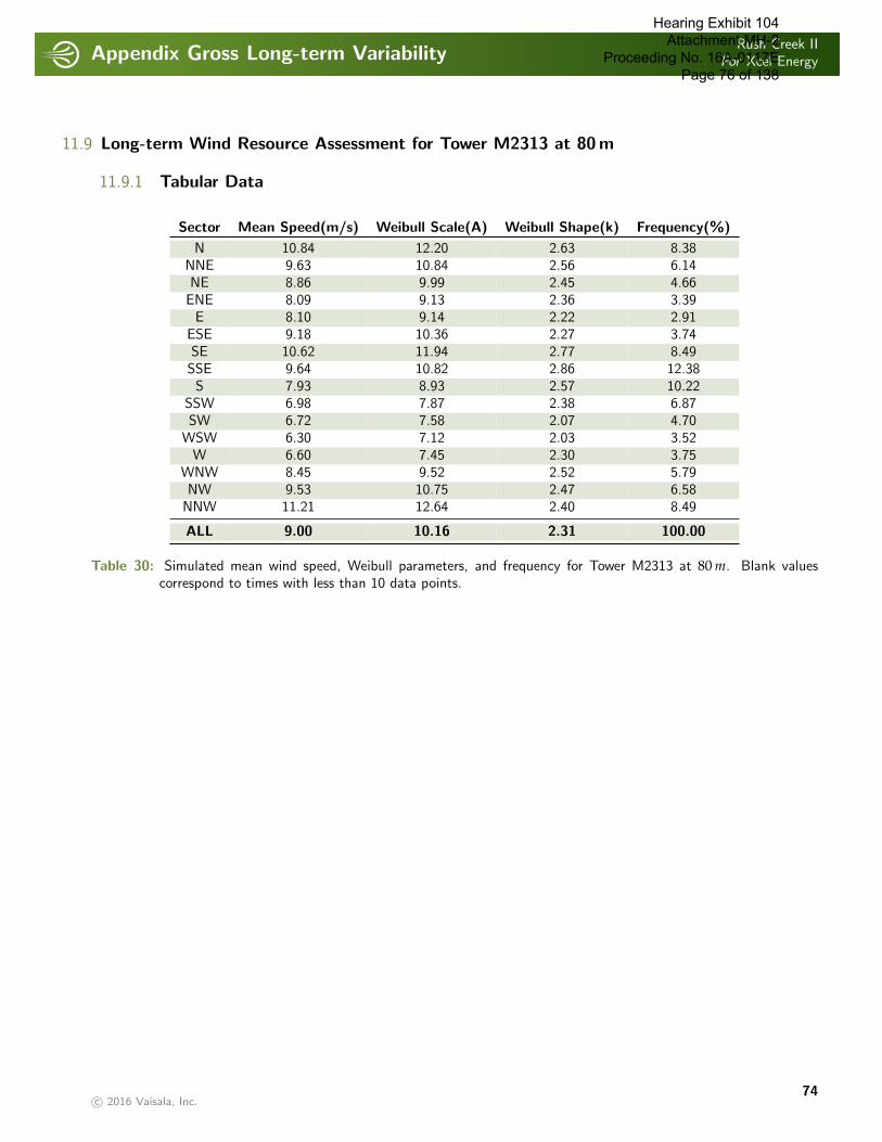
Appendix Gross Long-term VariabilityRush Creek II
For Xcel Energy
. . . . . . . . . . . . . . . . . . . . . . . . . . . . . . . . . . . . . . . . . . . . . . . . . . . . . . . . . . . . . . . . . . . . . . . . . . . . . . . . . . . . . . . . . . . . . . . . . . . . . . . . . . . . . . . . . .
11.9 Long-term Wind Resource Assessment for Tower M2313 at 80 m
11.9.1 Tabular Data
Sector Mean Speed(m/s) Weibull Scale(A) Weibull Shape(k) Frequency(%)
N 10.84 12.20 2.63 8.38NNE 9.63 10.84 2.56 6.14NE 8.86 9.99 2.45 4.66ENE 8.09 9.13 2.36 3.39E 8.10 9.14 2.22 2.91
ESE 9.18 10.36 2.27 3.74SE 10.62 11.94 2.77 8.49SSE 9.64 10.82 2.86 12.38S 7.93 8.93 2.57 10.22
SSW 6.98 7.87 2.38 6.87SW 6.72 7.58 2.07 4.70
WSW 6.30 7.12 2.03 3.52W 6.60 7.45 2.30 3.75
WNW 8.45 9.52 2.52 5.79NW 9.53 10.75 2.47 6.58
NNW 11.21 12.64 2.40 8.49
ALL 9.00 10.16 2.31 100.00
Table 30: Simulated mean wind speed, Weibull parameters, and frequency for Tower M2313 at 80 m. Blank valuescorrespond to times with less than 10 data points.
c© 2016 Vaisala, Inc.74
Hearing Exhibit 104 Attachment MH-2
Proceeding No. 16A-0117E Page 76 of 138

Appendix Gross Long-term VariabilityRush Creek II
For Xcel Energy
. . . . . . . . . . . . . . . . . . . . . . . . . . . . . . . . . . . . . . . . . . . . . . . . . . . . . . . . . . . . . . . . . . . . . . . . . . . . . . . . . . . . . . . . . . . . . . . . . . . . . . . . . . . . . . . . . .
Win
dSpee
dN
NN
EN
EEN
EE
ESE
SE
SSE
SSSW
SW
WSW
WW
NW
NW
NN
WA
ll(m
/s)
0-
0.5
0.00
0.00
0.00
0.00
0.00
0.00
0.00
0.00
0.00
0.00
0.00
0.00
0.00
0.00
0.00
0.00
0.01
0.5
-1.
50.
010.
020.
020.
020.
020.
030.
030.
040.
030.
020.
020.
010.
010.
020.
020.
020.
351.
5-
2.5
0.09
0.10
0.10
0.10
0.12
0.13
0.13
0.15
0.17
0.16
0.14
0.13
0.13
0.13
0.12
0.13
2.05
2.5
-3.
50.
190.
200.
200.
210.
200.
160.
190.
270.
430.
490.
430.
400.
360.
290.
250.
214.
493.
5-
4.5
0.26
0.28
0.26
0.25
0.22
0.20
0.25
0.38
0.64
0.73
0.67
0.56
0.44
0.36
0.29
0.26
6.03
4.5
-5.
50.
400.
410.
360.
310.
260.
270.
390.
640.
980.
980.
820.
670.
580.
480.
370.
388.
295.
5-
6.5
0.54
0.46
0.43
0.35
0.26
0.30
0.47
0.86
1.24
1.04
0.67
0.53
0.53
0.55
0.49
0.48
9.21
6.5
-7.
50.
610.
550.
500.
380.
300.
350.
601.
161.
430.
960.
510.
350.
480.
640.
620.
5910
.04
7.5
-8.
50.
680.
590.
490.
370.
280.
340.
671.
351.
410.
770.
390.
230.
370.
630.
670.
679.
938.
5-
9.5
0.72
0.59
0.46
0.32
0.26
0.32
0.71
1.44
1.22
0.58
0.27
0.16
0.27
0.60
0.69
0.75
9.38
9.5
-10
.50.
650.
510.
370.
250.
220.
300.
681.
320.
860.
380.
180.
110.
180.
510.
590.
677.
7810
.5-
11.5
0.59
0.44
0.31
0.20
0.17
0.24
0.69
1.08
0.57
0.23
0.14
0.08
0.12
0.42
0.51
0.58
6.38
11.5
-12
.50.
610.
440.
270.
170.
160.
230.
671.
010.
390.
150.
100.
070.
080.
350.
470.
565.
7412
.5-
13.5
0.62
0.40
0.26
0.16
0.14
0.23
0.73
0.94
0.29
0.11
0.10
0.06
0.06
0.30
0.43
0.58
5.41
13.5
-14
.50.
660.
370.
220.
130.
110.
210.
770.
730.
200.
090.
080.
050.
050.
230.
350.
584.
8314
.5-
15.5
0.50
0.27
0.16
0.07
0.06
0.14
0.54
0.40
0.11
0.07
0.05
0.03
0.02
0.12
0.22
0.48
3.25
15.5
-16
.50.
350.
170.
080.
040.
040.
090.
340.
190.
060.
040.
030.
020.
020.
060.
140.
321.
9916
.5-
17.5
0.25
0.13
0.06
0.02
0.02
0.06
0.20
0.14
0.03
0.02
0.03
0.01
0.01
0.03
0.09
0.25
1.36
17.5
-18
.50.
220.
080.
050.
010.
020.
050.
150.
100.
040.
020.
020.
020.
010.
020.
080.
261.
1418
.5-
19.5
0.18
0.06
0.03
0.01
0.01
0.04
0.11
0.07
0.03
0.02
0.02
0.01
0.01
0.01
0.06
0.22
0.88
19.5
-20
.50.
090.
030.
010.
010.
010.
020.
050.
040.
020.
010.
010.
000.
000.
010.
030.
130.
4620
.5-
21.5
0.05
0.01
0.00
0.00
0.00
0.01
0.02
0.02
0.01
0.00
0.00
0.00
0.00
0.00
0.02
0.07
0.23
21.5
-22
.50.
040.
010.
010.
000.
000.
010.
030.
030.
010.
010.
010.
000.
000.
010.
030.
100.
3022
.5-
23.5
0.04
0.00
0.00
0.00
0.00
0.01
0.02
0.02
0.01
0.00
0.00
0.00
0.00
0.01
0.02
0.09
0.23
23.5
-24
.50.
010.
000.
000.
000.
000.
000.
000.
000.
000.
000.
000.
000.
000.
000.
010.
020.
06>
24.5
0.02
0.00
0.00
0.00
0.00
0.01
0.01
0.01
0.01
0.00
0.00
0.00
0.00
0.01
0.02
0.11
0.20
Table
31:
Distr
ibution
ofsim
ula
ted
win
dsp
eed
bydirec
tion
for
Tow
erM
2313
at80
m.
c© 2016 Vaisala, Inc.75
Hearing Exhibit 104 Attachment MH-2
Proceeding No. 16A-0117E Page 77 of 138
Appendix Validation of Model ResultsRush Creek II
For Xcel Energy
. . . . . . . . . . . . . . . . . . . . . . . . . . . . . . . . . . . . . . . . . . . . . . . . . . . . . . . . . . . . . . . . . . . . . . . . . . . . . . . . . . . . . . . . . . . . . . . . . . . . . . . . . . . . . . . . . .
12 APPENDIX VALIDATION OF MODEL RESULTS. . . . . . . . . . . . . . . . . . . . . . . . . . . . . . . . . . . . . . . . . . . . . . . . . . . . . . . . . . . . . . . . . . . . . . . . . . . . . . . . . . . . . . . . . . . . . . . . . . . . . . . . . . . . . . . . . . . . . . . . . . . . . . . . . . . . . . . .
12.1 Validation of Model Results at Tower M2196
This section examines the quality of the NWP simulations used at a single point within the study area. For this section,the observations were taken at Tower M2196 (latitude 39.11318, longitude -103.2344).
The average observed wind speed (for all valid observational times) at 59.0 m during the 28 months of the period ofrecord (June, 2008 to September, 2010) is 8.51 m/s with an hourly standard deviation of 3.86 m/s at Tower M2196. Thiscompares to a modeled 59 m wind speed of 7.44 m/s with a 3.47 m/s standard deviation for these same times.
Based on a comparison of the NWP model output with observations from each of the meteorological towers for whichdata were provided, Model Output Statistics (MOS) was constructed. MOS uses a multilinear regression model designedto remove the bias and adjust the variance of the raw NWP simulated wind speed and direction. Applying this statisticalmodel to the simulated data at Tower M2196 results in a MOS-corrected mean value of 8.51 m/s and an hourly standarddeviation of 3.86 m/s.
This section presents a comparison of the simulated winds with the observations at the reference tower (Tower M2196).The focus of the verification is on the model’s ability to reproduce the observed variability of the wind resource at daily andmonthly time scales, while preserving the distribution of hourly wind speeds and the diurnal characteristics of the wind.
c© 2016 Vaisala, Inc.76
Hearing Exhibit 104 Attachment MH-2
Proceeding No. 16A-0117E Page 78 of 138
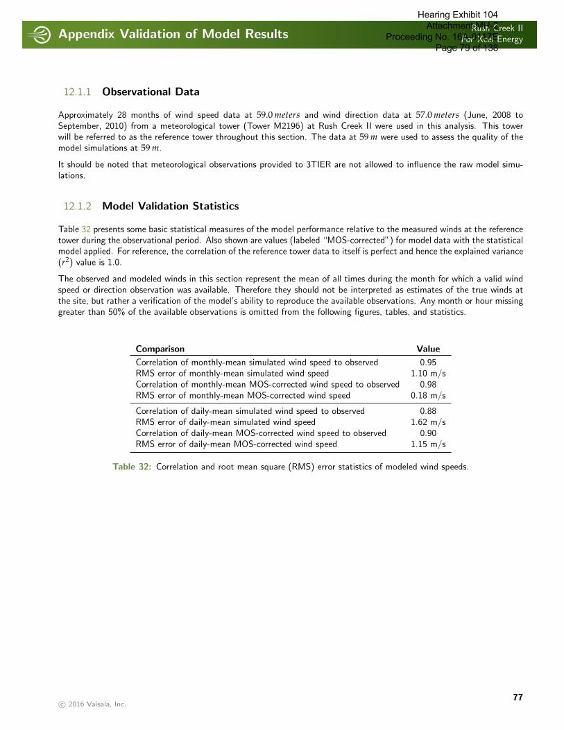
Appendix Validation of Model ResultsRush Creek II
For Xcel Energy
. . . . . . . . . . . . . . . . . . . . . . . . . . . . . . . . . . . . . . . . . . . . . . . . . . . . . . . . . . . . . . . . . . . . . . . . . . . . . . . . . . . . . . . . . . . . . . . . . . . . . . . . . . . . . . . . . .
12.1.1 Observational Data
Approximately 28 months of wind speed data at 59.0 meters and wind direction data at 57.0 meters (June, 2008 toSeptember, 2010) from a meteorological tower (Tower M2196) at Rush Creek II were used in this analysis. This towerwill be referred to as the reference tower throughout this section. The data at 59 m were used to assess the quality of themodel simulations at 59 m.
It should be noted that meteorological observations provided to 3TIER are not allowed to influence the raw model simu-lations.
12.1.2 Model Validation Statistics
Table 32 presents some basic statistical measures of the model performance relative to the measured winds at the referencetower during the observational period. Also shown are values (labeled “MOS-corrected”) for model data with the statisticalmodel applied. For reference, the correlation of the reference tower data to itself is perfect and hence the explained variance(r2) value is 1.0.
The observed and modeled winds in this section represent the mean of all times during the month for which a valid windspeed or direction observation was available. Therefore they should not be interpreted as estimates of the true winds atthe site, but rather a verification of the model’s ability to reproduce the available observations. Any month or hour missinggreater than 50% of the available observations is omitted from the following figures, tables, and statistics.
Comparison Value
Correlation of monthly-mean simulated wind speed to observed 0.95RMS error of monthly-mean simulated wind speed 1.10 m/sCorrelation of monthly-mean MOS-corrected wind speed to observed 0.98RMS error of monthly-mean MOS-corrected wind speed 0.18 m/s
Correlation of daily-mean simulated wind speed to observed 0.88RMS error of daily-mean simulated wind speed 1.62 m/sCorrelation of daily-mean MOS-corrected wind speed to observed 0.90RMS error of daily-mean MOS-corrected wind speed 1.15 m/s
Table 32: Correlation and root mean square (RMS) error statistics of modeled wind speeds.
c© 2016 Vaisala, Inc.77
Hearing Exhibit 104 Attachment MH-2
Proceeding No. 16A-0117E Page 79 of 138
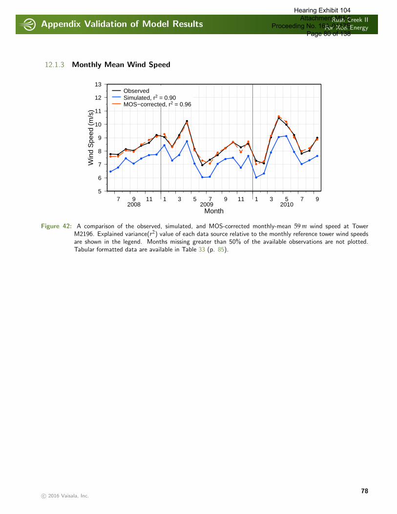
Appendix Validation of Model ResultsRush Creek II
For Xcel Energy
. . . . . . . . . . . . . . . . . . . . . . . . . . . . . . . . . . . . . . . . . . . . . . . . . . . . . . . . . . . . . . . . . . . . . . . . . . . . . . . . . . . . . . . . . . . . . . . . . . . . . . . . . . . . . . . . . .
12.1.3 Monthly Mean Wind Speed
7 9 11 1 3 5 7 9 11 1 3 5 7 9
Month2008 2009 2010
5
6
7
8
9
10
11
12
13W
ind
Spe
ed (
m/s
)ObservedSimulated, r2 = 0.90MOS−corrected, r2 = 0.96
Figure 42: A comparison of the observed, simulated, and MOS-corrected monthly-mean 59 m wind speed at TowerM2196. Explained variance(r2) value of each data source relative to the monthly reference tower wind speedsare shown in the legend. Months missing greater than 50% of the available observations are not plotted.Tabular formatted data are available in Table 33 (p. 85).
c© 2016 Vaisala, Inc.78
Hearing Exhibit 104 Attachment MH-2
Proceeding No. 16A-0117E Page 80 of 138
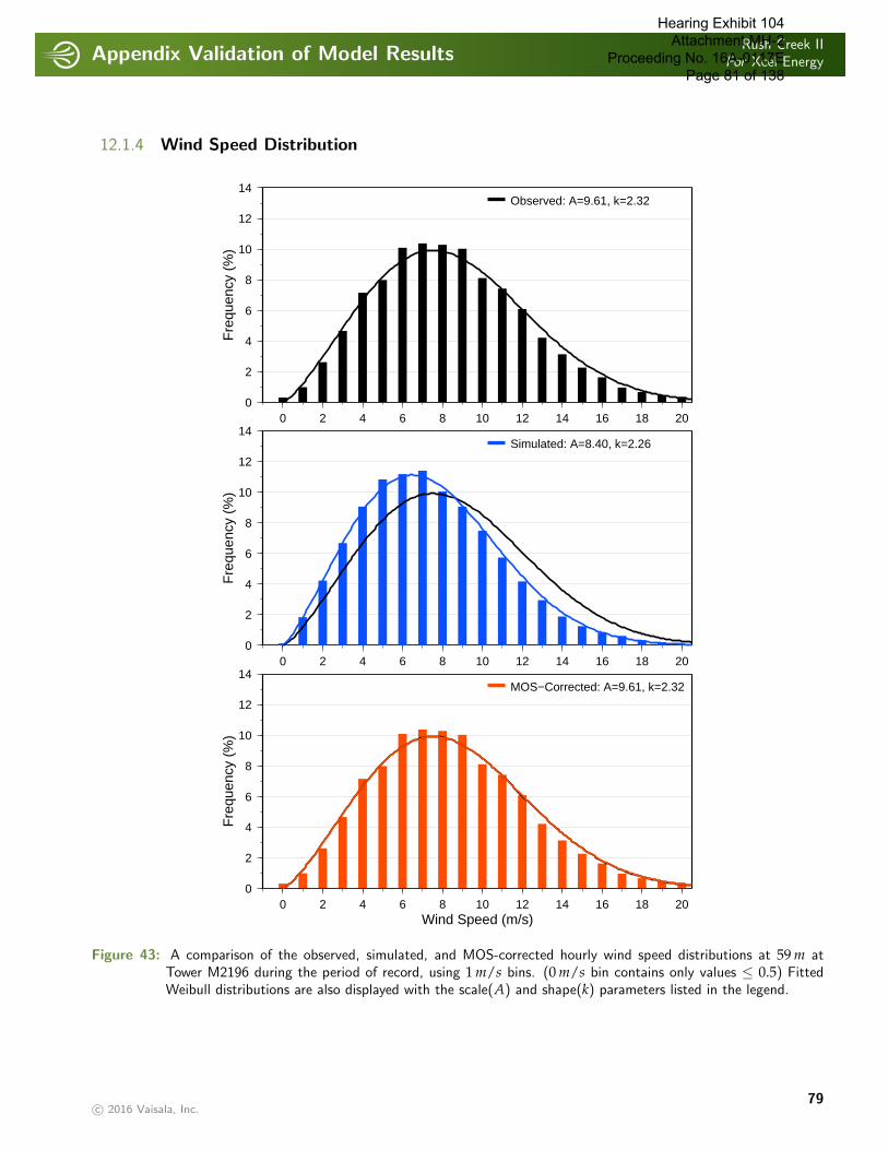
Appendix Validation of Model ResultsRush Creek II
For Xcel Energy
. . . . . . . . . . . . . . . . . . . . . . . . . . . . . . . . . . . . . . . . . . . . . . . . . . . . . . . . . . . . . . . . . . . . . . . . . . . . . . . . . . . . . . . . . . . . . . . . . . . . . . . . . . . . . . . . . .
12.1.4 Wind Speed Distribution
0 2 4 6 8 10 12 14 16 18 200
2
4
6
8
10
12
14
Fre
quen
cy (
%)
Observed: A=9.61, k=2.32
0 2 4 6 8 10 12 14 16 18 200
2
4
6
8
10
12
14
Fre
quen
cy (
%)
Simulated: A=8.40, k=2.26
0 2 4 6 8 10 12 14 16 18 20Wind Speed (m/s)
0
2
4
6
8
10
12
14
Fre
quen
cy (
%)
MOS−Corrected: A=9.61, k=2.32
Figure 43: A comparison of the observed, simulated, and MOS-corrected hourly wind speed distributions at 59 m atTower M2196 during the period of record, using 1 m/s bins. (0 m/s bin contains only values ≤ 0.5) FittedWeibull distributions are also displayed with the scale(A) and shape(k) parameters listed in the legend.
c© 2016 Vaisala, Inc.79
Hearing Exhibit 104 Attachment MH-2
Proceeding No. 16A-0117E Page 81 of 138
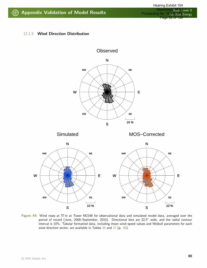
Appendix Validation of Model ResultsRush Creek II
For Xcel Energy
. . . . . . . . . . . . . . . . . . . . . . . . . . . . . . . . . . . . . . . . . . . . . . . . . . . . . . . . . . . . . . . . . . . . . . . . . . . . . . . . . . . . . . . . . . . . . . . . . . . . . . . . . . . . . . . . . .
12.1.5 Wind Direction Distribution
Observed
S 10 %
EW
N
S 10 %
EW
N
SW
NW
SE
NE
Simulated
S 10 %
EW
N
S 10 %
EW
N
SW
NW
SE
NE
MOS−Corrected
S 10 %
EW
N
S 10 %
EW
N
SW
NW
SE
NE
Figure 44: Wind roses at 57 m at Tower M2196 for observational data and simulated model data, averaged over theperiod of record (June, 2008–September, 2010). Directional bins are 22.5◦ wide, and the radial contourinterval is 10%. Tabular formatted data, including mean wind speed values and Weibull parameters for eachwind direction sector, are available in Tables 36 and 37 (p. 90).
c© 2016 Vaisala, Inc.80
Hearing Exhibit 104 Attachment MH-2
Proceeding No. 16A-0117E Page 82 of 138
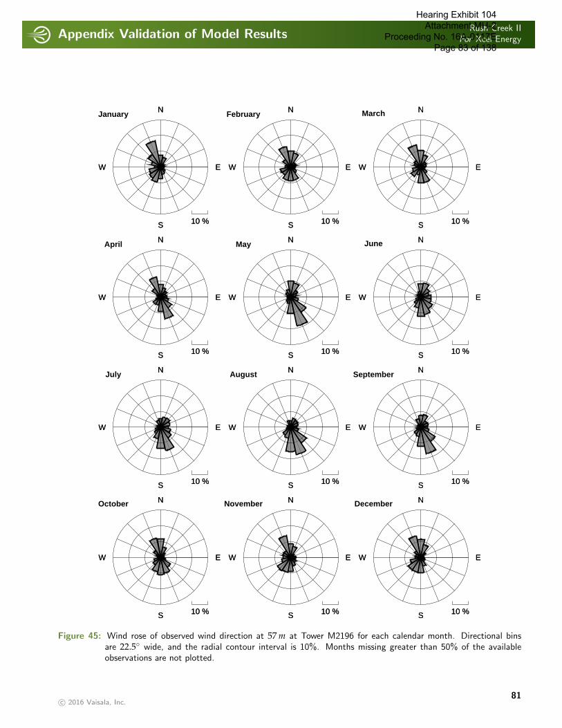
Appendix Validation of Model ResultsRush Creek II
For Xcel Energy
. . . . . . . . . . . . . . . . . . . . . . . . . . . . . . . . . . . . . . . . . . . . . . . . . . . . . . . . . . . . . . . . . . . . . . . . . . . . . . . . . . . . . . . . . . . . . . . . . . . . . . . . . . . . . . . . . .
S 10 %
EW
NOctober
S 10 %
EW
N
S 10 %
EW
NNovember
S 10 %
EW
N
S 10 %
EW
NDecember
S 10 %
EW
N
S 10 %
EW
NJuly
S 10 %
EW
N
S 10 %
EW
NAugust
S 10 %
EW
N
S 10 %
EW
NSeptember
S 10 %
EW
N
S 10 %
EW
NApril
S 10 %
EW
N
S 10 %
EW
NMay
S 10 %
EW
N
S 10 %
EW
NJune
S 10 %
EW
N
S 10 %
EW
NJanuary
S 10 %
EW
N
S 10 %
EW
NFebruary
S 10 %
EW
N
S 10 %
EW
NMarch
S 10 %
EW
N
Figure 45: Wind rose of observed wind direction at 57 m at Tower M2196 for each calendar month. Directional binsare 22.5◦ wide, and the radial contour interval is 10%. Months missing greater than 50% of the availableobservations are not plotted.
c© 2016 Vaisala, Inc.81
Hearing Exhibit 104 Attachment MH-2
Proceeding No. 16A-0117E Page 83 of 138
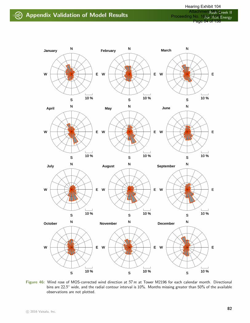
Appendix Validation of Model ResultsRush Creek II
For Xcel Energy
. . . . . . . . . . . . . . . . . . . . . . . . . . . . . . . . . . . . . . . . . . . . . . . . . . . . . . . . . . . . . . . . . . . . . . . . . . . . . . . . . . . . . . . . . . . . . . . . . . . . . . . . . . . . . . . . . .
S 10 %
EW
NOctober
S 10 %
EW
N
S 10 %
EW
NNovember
S 10 %
EW
N
S 10 %
EW
NDecember
S 10 %
EW
N
S 10 %
EW
NJuly
S 10 %
EW
N
S 10 %
EW
NAugust
S 10 %
EW
N
S 10 %
EW
NSeptember
S 10 %
EW
N
S 10 %
EW
NApril
S 10 %
EW
N
S 10 %
EW
NMay
S 10 %
EW
N
S 10 %
EW
NJune
S 10 %
EW
N
S 10 %
EW
NJanuary
S 10 %
EW
N
S 10 %
EW
NFebruary
S 10 %
EW
N
S 10 %
EW
NMarch
S 10 %
EW
N
Figure 46: Wind rose of MOS-corrected wind direction at 57 m at Tower M2196 for each calendar month. Directionalbins are 22.5◦ wide, and the radial contour interval is 10%. Months missing greater than 50% of the availableobservations are not plotted.
c© 2016 Vaisala, Inc.82
Hearing Exhibit 104 Attachment MH-2
Proceeding No. 16A-0117E Page 84 of 138

Appendix Validation of Model ResultsRush Creek II
For Xcel Energy
. . . . . . . . . . . . . . . . . . . . . . . . . . . . . . . . . . . . . . . . . . . . . . . . . . . . . . . . . . . . . . . . . . . . . . . . . . . . . . . . . . . . . . . . . . . . . . . . . . . . . . . . . . . . . . . . . .
12.1.6 Diurnal Variability of Wind Speed
0 4 8 12 16 20 24
Hour of Day (MST)
5
6
7
8
9
10
11
Win
d S
peed
(m
/s)
ObservedSimulatedMOS−corrected
Figure 47: A comparison of the diurnal cycle of observed, simulated, and MOS-corrected 59m wind speed at TowerM2196. Data are averaged over the period of record (June, 2008–September, 2010). Hours missing greaterthan 15% of the available observations are not plotted. The horizontal axis is Mountain Standard Time (MST).Tabular formatted data are available in Figures 49 and 50 (p. 86 and 87).
c© 2016 Vaisala, Inc.83
Hearing Exhibit 104 Attachment MH-2
Proceeding No. 16A-0117E Page 85 of 138
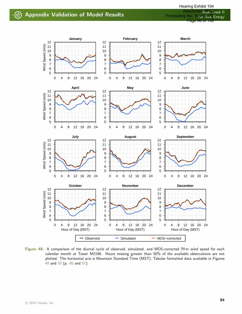
Appendix Validation of Model ResultsRush Creek II
For Xcel Energy
. . . . . . . . . . . . . . . . . . . . . . . . . . . . . . . . . . . . . . . . . . . . . . . . . . . . . . . . . . . . . . . . . . . . . . . . . . . . . . . . . . . . . . . . . . . . . . . . . . . . . . . . . . . . . . . . . .
January
0 4 8 12 16 20 24
56789
101112
Win
d S
peed
(m
/s)
February
0 4 8 12 16 20 24
56789
101112
March
0 4 8 12 16 20 24
56789
101112
April
0 4 8 12 16 20 24
56789
101112
Win
d S
peed
(m
/s)
May
0 4 8 12 16 20 24
56789
101112
June
0 4 8 12 16 20 24
56789
101112
July
0 4 8 12 16 20 24
56789
101112
Win
d S
peed
(m
/s)
August
0 4 8 12 16 20 24
56789
101112
September
0 4 8 12 16 20 24
56789
101112
October
0 4 8 12 16 20 24Hour of Day (MST)
56789
101112
Win
d S
peed
(m
/s)
November
0 4 8 12 16 20 24Hour of Day (MST)
56789
101112
Observed Simulated MOS−corrected
December
0 4 8 12 16 20 24Hour of Day (MST)
56789
101112
Figure 48: A comparison of the diurnal cycle of observed, simulated, and MOS-corrected 59 m wind speed for eachcalendar month at Tower M2196. Hours missing greater than 50% of the available observations are notplotted. The horizontal axis is Mountain Standard Time (MST). Tabular formatted data available in Figures49 and 50 (p. 86 and 87).
c© 2016 Vaisala, Inc.84
Hearing Exhibit 104 Attachment MH-2
Proceeding No. 16A-0117E Page 86 of 138
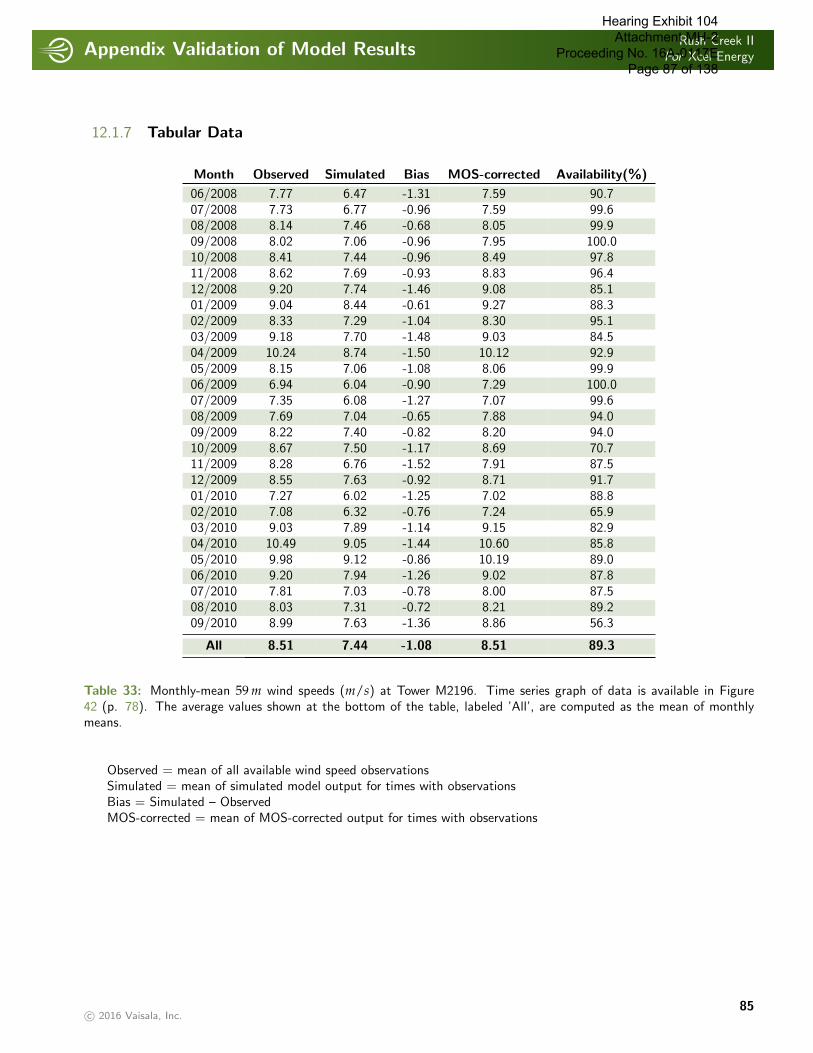
Appendix Validation of Model ResultsRush Creek II
For Xcel Energy
. . . . . . . . . . . . . . . . . . . . . . . . . . . . . . . . . . . . . . . . . . . . . . . . . . . . . . . . . . . . . . . . . . . . . . . . . . . . . . . . . . . . . . . . . . . . . . . . . . . . . . . . . . . . . . . . . .
12.1.7 Tabular Data
Month Observed Simulated Bias MOS-corrected Availability(%)
06/2008 7.77 6.47 -1.31 7.59 90.707/2008 7.73 6.77 -0.96 7.59 99.608/2008 8.14 7.46 -0.68 8.05 99.909/2008 8.02 7.06 -0.96 7.95 100.010/2008 8.41 7.44 -0.96 8.49 97.811/2008 8.62 7.69 -0.93 8.83 96.412/2008 9.20 7.74 -1.46 9.08 85.101/2009 9.04 8.44 -0.61 9.27 88.302/2009 8.33 7.29 -1.04 8.30 95.103/2009 9.18 7.70 -1.48 9.03 84.504/2009 10.24 8.74 -1.50 10.12 92.905/2009 8.15 7.06 -1.08 8.06 99.906/2009 6.94 6.04 -0.90 7.29 100.007/2009 7.35 6.08 -1.27 7.07 99.608/2009 7.69 7.04 -0.65 7.88 94.009/2009 8.22 7.40 -0.82 8.20 94.010/2009 8.67 7.50 -1.17 8.69 70.711/2009 8.28 6.76 -1.52 7.91 87.512/2009 8.55 7.63 -0.92 8.71 91.701/2010 7.27 6.02 -1.25 7.02 88.802/2010 7.08 6.32 -0.76 7.24 65.903/2010 9.03 7.89 -1.14 9.15 82.904/2010 10.49 9.05 -1.44 10.60 85.805/2010 9.98 9.12 -0.86 10.19 89.006/2010 9.20 7.94 -1.26 9.02 87.807/2010 7.81 7.03 -0.78 8.00 87.508/2010 8.03 7.31 -0.72 8.21 89.209/2010 8.99 7.63 -1.36 8.86 56.3
All 8.51 7.44 -1.08 8.51 89.3
Table 33: Monthly-mean 59 m wind speeds (m/s) at Tower M2196. Time series graph of data is available in Figure42 (p. 78). The average values shown at the bottom of the table, labeled ’All’, are computed as the mean of monthlymeans.
Observed = mean of all available wind speed observationsSimulated = mean of simulated model output for times with observationsBias = Simulated – ObservedMOS-corrected = mean of MOS-corrected output for times with observations
c© 2016 Vaisala, Inc.85
Hearing Exhibit 104 Attachment MH-2
Proceeding No. 16A-0117E Page 87 of 138
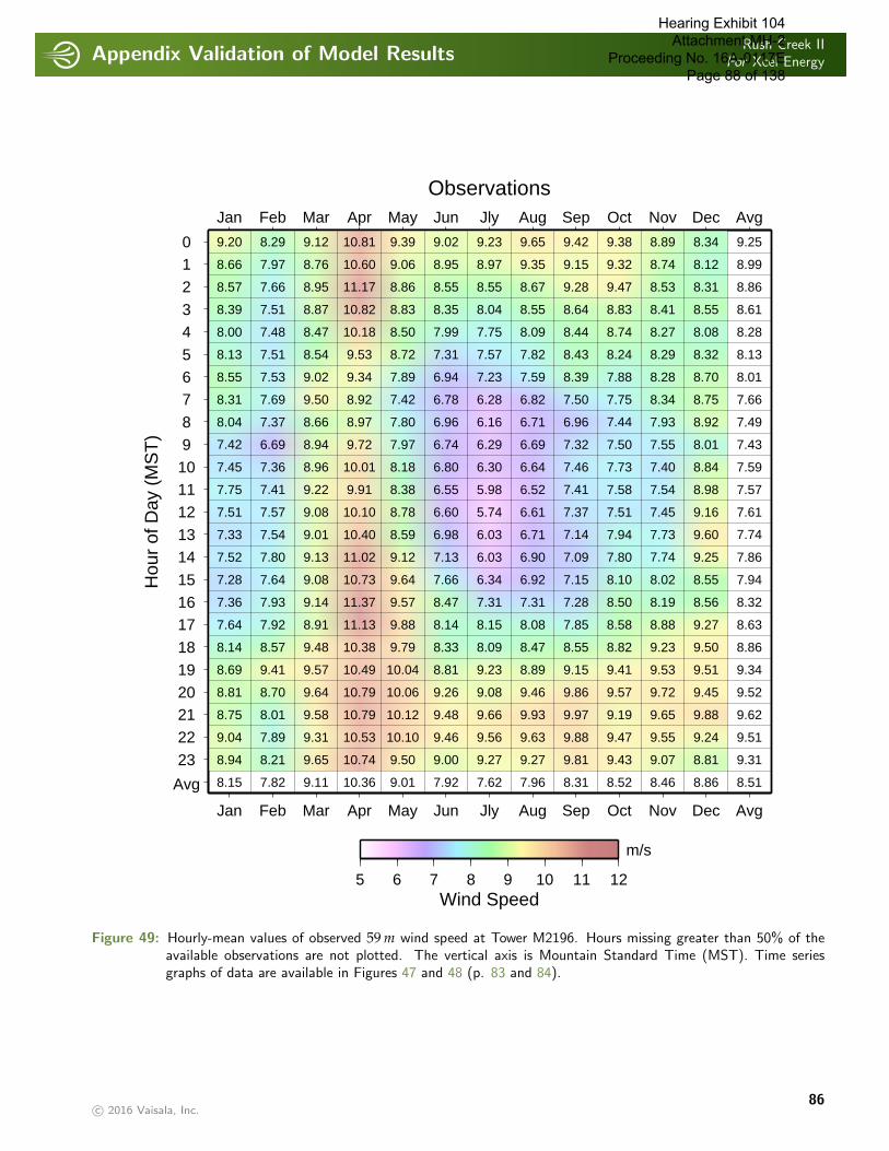
Appendix Validation of Model ResultsRush Creek II
For Xcel Energy
. . . . . . . . . . . . . . . . . . . . . . . . . . . . . . . . . . . . . . . . . . . . . . . . . . . . . . . . . . . . . . . . . . . . . . . . . . . . . . . . . . . . . . . . . . . . . . . . . . . . . . . . . . . . . . . . . .
Observations
Hou
r of
Day
(M
ST
)
012
34
567
89101112
1314
151617
1819202122
23
Avg
Jan
Jan
Feb
Feb
Mar
Mar
Apr
Apr
May
May
Jun
Jun
Jly
Jly
Aug
Aug
Sep
Sep
Oct
Oct
Nov
Nov
Dec
Dec
Avg
Avg
7.64
8.14
8.69
8.81
8.75
9.04
8.94
9.20
8.66
8.57
8.39
8.00
8.13
8.55
8.31
8.04
7.42
7.45
7.75
7.51
7.33
7.52
7.28
7.36
8.15
7.92
8.57
9.41
8.70
8.01
7.89
8.21
8.29
7.97
7.66
7.51
7.48
7.51
7.53
7.69
7.37
6.69
7.36
7.41
7.57
7.54
7.80
7.64
7.93
7.82
8.91
9.48
9.57
9.64
9.58
9.31
9.65
9.12
8.76
8.95
8.87
8.47
8.54
9.02
9.50
8.66
8.94
8.96
9.22
9.08
9.01
9.13
9.08
9.14
9.11
11.13
10.38
10.49
10.79
10.79
10.53
10.74
10.81
10.60
11.17
10.82
10.18
9.53
9.34
8.92
8.97
9.72
10.01
9.91
10.10
10.40
11.02
10.73
11.37
10.36
9.88
9.79
10.04
10.06
10.12
10.10
9.50
9.39
9.06
8.86
8.83
8.50
8.72
7.89
7.42
7.80
7.97
8.18
8.38
8.78
8.59
9.12
9.64
9.57
9.01
8.14
8.33
8.81
9.26
9.48
9.46
9.00
9.02
8.95
8.55
8.35
7.99
7.31
6.94
6.78
6.96
6.74
6.80
6.55
6.60
6.98
7.13
7.66
8.47
7.92
8.15
8.09
9.23
9.08
9.66
9.56
9.27
9.23
8.97
8.55
8.04
7.75
7.57
7.23
6.28
6.16
6.29
6.30
5.98
5.74
6.03
6.03
6.34
7.31
7.62
8.08
8.47
8.89
9.46
9.93
9.63
9.27
9.65
9.35
8.67
8.55
8.09
7.82
7.59
6.82
6.71
6.69
6.64
6.52
6.61
6.71
6.90
6.92
7.31
7.96
7.85
8.55
9.15
9.86
9.97
9.88
9.81
9.42
9.15
9.28
8.64
8.44
8.43
8.39
7.50
6.96
7.32
7.46
7.41
7.37
7.14
7.09
7.15
7.28
8.31
8.58
8.82
9.41
9.57
9.19
9.47
9.43
9.38
9.32
9.47
8.83
8.74
8.24
7.88
7.75
7.44
7.50
7.73
7.58
7.51
7.94
7.80
8.10
8.50
8.52
8.88
9.23
9.53
9.72
9.65
9.55
9.07
8.89
8.74
8.53
8.41
8.27
8.29
8.28
8.34
7.93
7.55
7.40
7.54
7.45
7.73
7.74
8.02
8.19
8.46
9.27
9.50
9.51
9.45
9.88
9.24
8.81
8.34
8.12
8.31
8.55
8.08
8.32
8.70
8.75
8.92
8.01
8.84
8.98
9.16
9.60
9.25
8.55
8.56
8.86
8.63
8.86
9.34
9.52
9.62
9.51
9.31
9.25
8.99
8.86
8.61
8.28
8.13
8.01
7.66
7.49
7.43
7.59
7.57
7.61
7.74
7.86
7.94
8.32
8.51
5 6 7 8 9 10 11 12Wind Speed
m/s
Figure 49: Hourly-mean values of observed 59 m wind speed at Tower M2196. Hours missing greater than 50% of theavailable observations are not plotted. The vertical axis is Mountain Standard Time (MST). Time seriesgraphs of data are available in Figures 47 and 48 (p. 83 and 84).
c© 2016 Vaisala, Inc.86
Hearing Exhibit 104 Attachment MH-2
Proceeding No. 16A-0117E Page 88 of 138
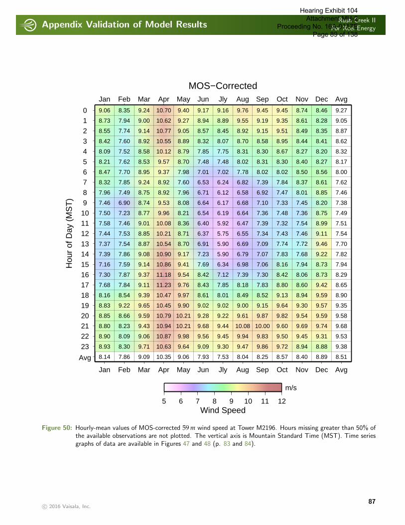
Appendix Validation of Model ResultsRush Creek II
For Xcel Energy
. . . . . . . . . . . . . . . . . . . . . . . . . . . . . . . . . . . . . . . . . . . . . . . . . . . . . . . . . . . . . . . . . . . . . . . . . . . . . . . . . . . . . . . . . . . . . . . . . . . . . . . . . . . . . . . . . .
MOS−Corrected
Hou
r of
Day
(M
ST
)
012
34
567
89
101112
1314
151617
1819202122
23
Avg
Jan
Jan
Feb
Feb
Mar
Mar
Apr
Apr
May
May
Jun
Jun
Jly
Jly
Aug
Aug
Sep
Sep
Oct
Oct
Nov
Nov
Dec
Dec
Avg
Avg
7.68
8.16
8.83
8.85
8.80
8.90
8.93
9.06
8.73
8.55
8.42
8.09
8.21
8.47
8.32
7.96
7.46
7.50
7.58
7.44
7.37
7.39
7.16
7.30
8.14
7.84
8.54
9.22
8.66
8.23
8.09
8.30
8.35
7.94
7.74
7.60
7.52
7.62
7.70
7.85
7.49
6.90
7.23
7.46
7.53
7.54
7.86
7.59
7.87
7.86
9.11
9.39
9.65
9.59
9.43
9.06
9.71
9.24
9.00
9.14
8.92
8.58
8.53
8.95
9.24
8.75
8.74
8.77
9.01
8.85
8.87
9.08
9.14
9.37
9.09
11.23
10.47
10.45
10.79
10.94
10.87
10.63
10.70
10.62
10.77
10.55
10.12
9.57
9.37
8.92
8.92
9.53
9.96
10.08
10.21
10.54
10.90
10.86
11.18
10.35
9.76
9.97
9.90
10.21
10.21
9.98
9.64
9.40
9.27
9.05
8.89
8.79
8.70
7.98
7.60
7.96
8.08
8.21
8.36
8.71
8.70
9.17
9.41
9.54
9.06
8.43
8.61
9.02
9.28
9.68
9.56
9.09
9.17
8.94
8.57
8.32
7.85
7.48
7.01
6.53
6.71
6.64
6.54
6.40
6.37
6.91
7.23
7.69
8.42
7.93
7.85
8.01
9.02
9.22
9.44
9.45
9.30
9.16
8.89
8.45
8.07
7.75
7.48
7.02
6.24
6.12
6.17
6.19
5.92
5.75
5.90
5.90
6.34
7.12
7.53
8.18
8.49
9.00
9.61
10.08
9.94
9.47
9.76
9.55
8.92
8.70
8.31
8.02
7.78
6.82
6.58
6.68
6.64
6.47
6.55
6.69
6.79
6.98
7.39
8.04
7.83
8.52
9.15
9.87
10.00
9.83
9.86
9.45
9.19
9.15
8.58
8.30
8.31
8.02
7.39
6.92
7.10
7.36
7.39
7.34
7.09
7.07
7.06
7.30
8.25
8.80
9.13
9.64
9.82
9.60
9.50
9.72
9.45
9.35
9.51
8.95
8.67
8.30
8.02
7.84
7.47
7.33
7.48
7.32
7.43
7.74
7.83
8.16
8.42
8.57
8.60
8.94
9.30
9.54
9.69
9.45
8.94
8.74
8.61
8.49
8.44
8.27
8.40
8.50
8.37
8.01
7.45
7.36
7.54
7.46
7.72
7.68
7.94
8.06
8.40
9.42
9.59
9.57
9.59
9.74
9.31
8.88
8.46
8.28
8.35
8.41
8.20
8.27
8.56
8.61
8.85
8.20
8.75
8.99
9.11
9.46
9.22
8.73
8.73
8.89
8.65
8.90
9.35
9.58
9.68
9.53
9.38
9.27
9.05
8.87
8.62
8.32
8.17
8.00
7.62
7.46
7.38
7.49
7.51
7.54
7.70
7.82
7.94
8.29
8.51
5 6 7 8 9 10 11 12Wind Speed
m/s
Figure 50: Hourly-mean values of MOS-corrected 59 m wind speed at Tower M2196. Hours missing greater than 50% ofthe available observations are not plotted. The vertical axis is Mountain Standard Time (MST). Time seriesgraphs of data are available in Figures 47 and 48 (p. 83 and 84).
c© 2016 Vaisala, Inc.87
Hearing Exhibit 104 Attachment MH-2
Proceeding No. 16A-0117E Page 89 of 138
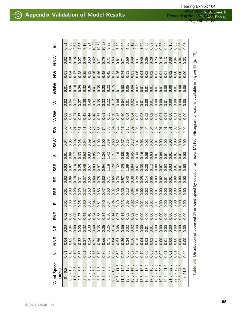
Appendix Validation of Model ResultsRush Creek II
For Xcel Energy
. . . . . . . . . . . . . . . . . . . . . . . . . . . . . . . . . . . . . . . . . . . . . . . . . . . . . . . . . . . . . . . . . . . . . . . . . . . . . . . . . . . . . . . . . . . . . . . . . . . . . . . . . . . . . . . . . .
Win
dSpee
dN
NN
EN
EEN
EE
ESE
SE
SSE
SSSW
SW
WSW
WW
NW
NW
NN
WA
ll(m
/s)
0-
0.5
0.01
0.04
0.03
0.02
0.01
0.01
0.02
0.03
0.01
0.04
0.00
0.03
0.02
0.01
0.01
0.02
0.31
0.5
-1.
50.
100.
050.
040.
080.
030.
030.
090.
070.
090.
060.
070.
080.
040.
060.
040.
080.
981.
5-
2.5
0.19
0.17
0.09
0.08
0.16
0.20
0.18
0.14
0.17
0.14
0.21
0.21
0.17
0.18
0.17
0.16
2.62
2.5
-3.
50.
360.
320.
200.
270.
250.
290.
310.
250.
330.
280.
310.
370.
270.
290.
280.
274.
653.
5-
4.5
0.51
0.37
0.32
0.41
0.50
0.37
0.37
0.48
0.62
0.64
0.51
0.48
0.38
0.32
0.35
0.49
7.13
4.5
-5.
50.
530.
540.
300.
400.
370.
530.
560.
570.
830.
690.
580.
440.
400.
360.
320.
537.
945.
5-
6.5
0.76
0.72
0.40
0.54
0.54
0.40
0.69
0.83
0.95
1.07
0.76
0.48
0.31
0.41
0.56
0.62
10.0
56.
5-
7.5
0.79
0.56
0.35
0.38
0.51
0.53
0.75
0.97
1.12
1.00
0.85
0.55
0.35
0.35
0.56
0.71
10.3
47.
5-
8.5
0.86
0.66
0.26
0.34
0.40
0.47
0.82
0.94
1.24
1.00
0.74
0.61
0.33
0.28
0.48
0.79
10.2
38.
5-
9.5
0.83
0.71
0.25
0.30
0.34
0.50
0.71
1.18
1.42
0.79
0.80
0.55
0.22
0.22
0.45
0.71
9.99
9.5
-10
.50.
790.
640.
140.
140.
240.
370.
661.
201.
210.
630.
540.
300.
120.
150.
310.
638.
0810
.5-
11.5
0.69
0.53
0.08
0.07
0.19
0.30
0.70
1.32
1.16
0.52
0.44
0.15
0.06
0.11
0.26
0.81
7.39
11.5
-12
.50.
560.
360.
060.
110.
130.
300.
571.
290.
880.
370.
270.
100.
040.
080.
240.
716.
0612
.5-
13.5
0.55
0.24
0.02
0.02
0.05
0.13
0.40
1.09
0.59
0.15
0.15
0.04
0.01
0.05
0.13
0.59
4.20
13.5
-14
.50.
370.
160.
020.
020.
020.
040.
380.
840.
450.
120.
090.
040.
020.
040.
030.
483.
1214
.5-
15.5
0.31
0.10
0.00
0.00
0.03
0.04
0.28
0.67
0.30
0.07
0.06
0.02
0.01
0.02
0.06
0.31
2.25
15.5
-16
.50.
190.
040.
000.
000.
010.
020.
250.
380.
160.
030.
070.
030.
010.
010.
040.
401.
6216
.5-
17.5
0.09
0.03
0.01
0.00
0.01
0.02
0.14
0.20
0.08
0.03
0.04
0.02
0.00
0.01
0.03
0.26
0.96
17.5
-18
.50.
030.
020.
010.
000.
010.
000.
060.
120.
030.
020.
040.
020.
010.
010.
020.
280.
6718
.5-
19.5
0.04
0.01
0.00
0.00
0.01
0.01
0.03
0.08
0.01
0.01
0.02
0.00
0.00
0.01
0.01
0.23
0.45
19.5
-20
.50.
020.
000.
000.
000.
000.
000.
020.
070.
040.
000.
010.
010.
000.
010.
010.
160.
3520
.5-
21.5
0.01
0.01
0.00
0.00
0.00
0.00
0.01
0.03
0.01
0.00
0.01
0.01
0.01
0.00
0.01
0.13
0.22
21.5
-22
.50.
010.
000.
000.
000.
000.
000.
010.
030.
010.
000.
010.
000.
000.
000.
020.
080.
1622
.5-
23.5
0.01
0.00
0.00
0.00
0.00
0.00
0.00
0.01
0.01
0.00
0.00
0.01
0.00
0.01
0.00
0.04
0.08
23.5
-24
.50.
000.
000.
000.
000.
000.
000.
000.
010.
010.
000.
000.
000.
000.
000.
000.
040.
06>
24.5
0.00
0.00
0.00
0.00
0.00
0.00
0.00
0.00
0.00
0.00
0.00
0.00
0.00
0.00
0.00
0.03
0.03
Table
34:
Distr
ibution
ofob
serv
ed59
mw
ind
spee
dby
direc
tion
atTow
erM
2196
.H
isto
gram
ofdat
ais
avai
lable
inFig
ure
43(p
.79
).
c© 2016 Vaisala, Inc.88
Hearing Exhibit 104 Attachment MH-2
Proceeding No. 16A-0117E Page 90 of 138

Appendix Validation of Model ResultsRush Creek II
For Xcel Energy
. . . . . . . . . . . . . . . . . . . . . . . . . . . . . . . . . . . . . . . . . . . . . . . . . . . . . . . . . . . . . . . . . . . . . . . . . . . . . . . . . . . . . . . . . . . . . . . . . . . . . . . . . . . . . . . . . .
Win
dSpee
dN
NN
EN
EEN
EE
ESE
SE
SSE
SSSW
SW
WSW
WW
NW
NW
NN
WA
ll(m
/s)
0-
0.5
0.03
0.02
0.01
0.01
0.01
0.01
0.04
0.03
0.02
0.01
0.01
0.03
0.00
0.02
0.03
0.02
0.31
0.5
-1.
50.
080.
070.
070.
060.
050.
070.
040.
070.
080.
030.
040.
040.
070.
080.
050.
090.
981.
5-
2.5
0.19
0.24
0.16
0.18
0.15
0.15
0.18
0.15
0.17
0.15
0.18
0.15
0.16
0.13
0.15
0.14
2.62
2.5
-3.
50.
280.
210.
340.
360.
320.
270.
360.
250.
310.
300.
330.
380.
300.
270.
160.
224.
653.
5-
4.5
0.34
0.43
0.37
0.38
0.42
0.43
0.40
0.40
0.52
0.57
0.66
0.64
0.51
0.41
0.33
0.30
7.13
4.5
-5.
50.
370.
290.
300.
500.
290.
380.
440.
490.
710.
890.
840.
680.
490.
450.
390.
437.
945.
5-
6.5
0.59
0.50
0.46
0.56
0.44
0.38
0.60
0.68
1.09
1.27
0.90
0.66
0.50
0.50
0.32
0.61
10.0
56.
5-
7.5
0.76
0.53
0.43
0.37
0.42
0.41
0.53
1.00
1.36
1.44
0.71
0.40
0.50
0.46
0.44
0.59
10.3
47.
5-
8.5
0.72
0.55
0.37
0.38
0.43
0.42
0.73
1.14
1.44
1.22
0.47
0.34
0.43
0.40
0.54
0.68
10.2
58.
5-
9.5
0.82
0.56
0.39
0.33
0.25
0.40
0.67
1.43
1.54
0.92
0.38
0.20
0.26
0.41
0.54
0.88
9.99
9.5
-10
.50.
720.
520.
320.
180.
250.
290.
661.
251.
210.
540.
190.
150.
270.
400.
390.
738.
0810
.5-
11.5
0.82
0.42
0.20
0.10
0.13
0.31
0.69
1.31
1.16
0.45
0.20
0.11
0.13
0.27
0.41
0.68
7.38
11.5
-12
.50.
610.
430.
190.
090.
070.
200.
551.
360.
880.
290.
140.
080.
090.
200.
330.
556.
0612
.5-
13.5
0.45
0.30
0.05
0.03
0.05
0.11
0.50
1.17
0.51
0.19
0.14
0.04
0.05
0.06
0.14
0.42
4.20
13.5
-14
.50.
400.
230.
040.
000.
040.
050.
380.
790.
380.
080.
100.
080.
030.
040.
080.
413.
1214
.5-
15.5
0.31
0.11
0.03
0.01
0.02
0.02
0.19
0.67
0.27
0.07
0.04
0.02
0.03
0.02
0.07
0.39
2.25
15.5
-16
.50.
160.
070.
010.
000.
010.
020.
210.
430.
080.
060.
040.
040.
010.
010.
040.
441.
6216
.5-
17.5
0.15
0.02
0.02
0.00
0.01
0.01
0.08
0.21
0.04
0.01
0.02
0.03
0.00
0.01
0.01
0.36
0.96
17.5
-18
.50.
050.
010.
020.
000.
000.
000.
070.
150.
020.
020.
020.
010.
000.
010.
020.
280.
6718
.5-
19.5
0.08
0.01
0.00
0.00
0.00
0.01
0.01
0.11
0.02
0.01
0.03
0.01
0.01
0.00
0.01
0.16
0.45
19.5
-20
.50.
030.
000.
000.
000.
000.
000.
020.
080.
020.
020.
030.
010.
000.
000.
010.
140.
3520
.5-
21.5
0.01
0.00
0.00
0.00
0.00
0.01
0.02
0.04
0.01
0.02
0.01
0.00
0.01
0.00
0.02
0.09
0.22
21.5
-22
.50.
000.
000.
000.
000.
000.
010.
010.
020.
020.
020.
010.
000.
010.
010.
000.
060.
1622
.5-
23.5
0.00
0.00
0.00
0.00
0.00
0.00
0.00
0.01
0.01
0.01
0.00
0.00
0.00
0.00
0.01
0.06
0.08
23.5
-24
.50.
000.
000.
000.
000.
000.
000.
000.
000.
020.
000.
000.
000.
000.
000.
000.
040.
06>
24.5
0.00
0.00
0.00
0.00
0.00
0.00
0.00
0.02
0.01
0.00
0.00
0.00
0.00
0.00
0.00
0.01
0.03
Table
35:
Distr
ibution
ofM
OS-c
orre
cted
59m
win
dsp
eed
bydirec
tion
atTow
erM
2196
.A
llm
odel
valu
esar
eco
mpute
don
lyfo
rtim
esw
ith
valid
obse
rvat
ions.
Histo
gram
ofdat
ais
avai
lable
inFig
ure
43(p
.79
).
c© 2016 Vaisala, Inc.89
Hearing Exhibit 104 Attachment MH-2
Proceeding No. 16A-0117E Page 91 of 138

Appendix Validation of Model ResultsRush Creek II
For Xcel Energy
. . . . . . . . . . . . . . . . . . . . . . . . . . . . . . . . . . . . . . . . . . . . . . . . . . . . . . . . . . . . . . . . . . . . . . . . . . . . . . . . . . . . . . . . . . . . . . . . . . . . . . . . . . . . . . . . . .
Sector Mean Speed(m/s) Weibull Scale(A) Weibull Shape(k) Frequency(%)
N 8.90 10.03 2.49 8.60NNE 8.05 9.07 2.55 6.27NE 6.43 7.25 2.42 2.58ENE 6.31 7.11 2.51 3.18E 6.82 7.69 2.42 3.80
ESE 7.48 8.44 2.46 4.55SE 9.10 10.26 2.48 8.00SSE 10.17 11.41 2.85 12.79S 8.93 10.04 2.74 11.74
SSW 7.60 8.55 2.69 7.64SW 7.78 8.78 2.41 6.61
WSW 6.88 7.77 2.23 4.55W 6.04 6.82 2.22 2.78
WNW 6.52 7.36 2.08 2.98NW 7.65 8.64 2.27 4.38
NNW 10.52 11.87 2.25 9.56
ALL 8.51 9.61 2.32 100.00
Table 36: Observed 59 m mean wind speed, Weibull parameters, and frequency at Tower M2196. Blank values correspondto times with less than 10 data points. Wind rose of data is available in Figure 44 (p. 80).
Sector Mean Speed(m/s) Weibull Scale(A) Weibull Shape(k) Frequency(%)
N 9.35 10.53 2.57 7.95NNE 8.34 9.40 2.50 5.51NE 7.06 7.97 2.31 3.78ENE 6.18 6.96 2.49 3.53E 6.59 7.44 2.38 3.34
ESE 7.31 8.25 2.31 3.95SE 9.09 10.25 2.47 7.37SSE 10.31 11.56 2.91 13.25S 8.76 9.83 2.82 11.88
SSW 7.58 8.53 2.62 8.58SW 6.98 7.88 2.15 5.47
WSW 6.35 7.17 2.06 4.12W 6.62 7.47 2.27 3.85
WNW 7.17 8.09 2.39 4.15NW 8.17 9.22 2.39 4.49
NNW 10.68 12.05 2.33 8.78
ALL 8.51 9.61 2.32 100.00
Table 37: MOS-corrected 59 m mean wind speed, Weibull parameters, and frequency at Tower M2196. All MOS-correctedmodel values are computed only for times with valid observations; blank values correspond to times with lessthan 10 data points. Wind rose of data is available in Figure 44 (p. 80).
c© 2016 Vaisala, Inc.90
Hearing Exhibit 104 Attachment MH-2
Proceeding No. 16A-0117E Page 92 of 138

Appendix Validation of Model ResultsRush Creek II
For Xcel Energy
. . . . . . . . . . . . . . . . . . . . . . . . . . . . . . . . . . . . . . . . . . . . . . . . . . . . . . . . . . . . . . . . . . . . . . . . . . . . . . . . . . . . . . . . . . . . . . . . . . . . . . . . . . . . . . . . . .
12.2 Validation of Model Results at Tower M2202
This section examines the quality of the NWP simulations used at a single point within the study area. For this section,the observations were taken at Tower M2202 (latitude 39.13467, longitude -103.18216).
The average observed wind speed (for all valid observational times) at 59.0 m during the 27 months of the period of record(June, 2008 to August, 2010) is 8.23 m/s with an hourly standard deviation of 3.90 m/s at Tower M2202. This comparesto a modeled 59 m wind speed of 7.23 m/s with a 3.34 m/s standard deviation for these same times.
Based on a comparison of the NWP model output with observations from each of the meteorological towers for whichdata were provided, Model Output Statistics (MOS) was constructed. MOS uses a multilinear regression model designedto remove the bias and adjust the variance of the raw NWP simulated wind speed and direction. Applying this statisticalmodel to the simulated data at Tower M2202 results in a MOS-corrected mean value of 8.24 m/s and an hourly standarddeviation of 3.90 m/s.
This section presents a comparison of the simulated winds with the observations at the reference tower (Tower M2202).The focus of the verification is on the model’s ability to reproduce the observed variability of the wind resource at daily andmonthly time scales, while preserving the distribution of hourly wind speeds and the diurnal characteristics of the wind.
c© 2016 Vaisala, Inc.91
Hearing Exhibit 104 Attachment MH-2
Proceeding No. 16A-0117E Page 93 of 138

Appendix Validation of Model ResultsRush Creek II
For Xcel Energy
. . . . . . . . . . . . . . . . . . . . . . . . . . . . . . . . . . . . . . . . . . . . . . . . . . . . . . . . . . . . . . . . . . . . . . . . . . . . . . . . . . . . . . . . . . . . . . . . . . . . . . . . . . . . . . . . . .
12.2.1 Observational Data
Approximately 27 months of wind speed data at 59.0 meters and wind direction data at 57.0 meters (June, 2008 to August,2010) from a meteorological tower (Tower M2202) at Rush Creek II were used in this analysis. This tower will be referred toas the reference tower throughout this section. The data at 59 m were used to assess the quality of the model simulationsat 59 m.
It should be noted that meteorological observations provided to 3TIER are not allowed to influence the raw model simu-lations.
12.2.2 Model Validation Statistics
Table 38 presents some basic statistical measures of the model performance relative to the measured winds at the referencetower during the observational period. Also shown are values (labeled “MOS-corrected”) for model data with the statisticalmodel applied. For reference, the correlation of the reference tower data to itself is perfect and hence the explained variance(r2) value is 1.0.
The observed and modeled winds in this section represent the mean of all times during the month for which a valid windspeed or direction observation was available. Therefore they should not be interpreted as estimates of the true winds atthe site, but rather a verification of the model’s ability to reproduce the available observations. Any month or hour missinggreater than 50% of the available observations is omitted from the following figures, tables, and statistics.
Comparison Value
Correlation of monthly-mean simulated wind speed to observed 0.95RMS error of monthly-mean simulated wind speed 1.04 m/sCorrelation of monthly-mean MOS-corrected wind speed to observed 0.98RMS error of monthly-mean MOS-corrected wind speed 0.20 m/s
Correlation of daily-mean simulated wind speed to observed 0.88RMS error of daily-mean simulated wind speed 1.62 m/sCorrelation of daily-mean MOS-corrected wind speed to observed 0.90RMS error of daily-mean MOS-corrected wind speed 1.20 m/s
Table 38: Correlation and root mean square (RMS) error statistics of modeled wind speeds.
c© 2016 Vaisala, Inc.92
Hearing Exhibit 104 Attachment MH-2
Proceeding No. 16A-0117E Page 94 of 138
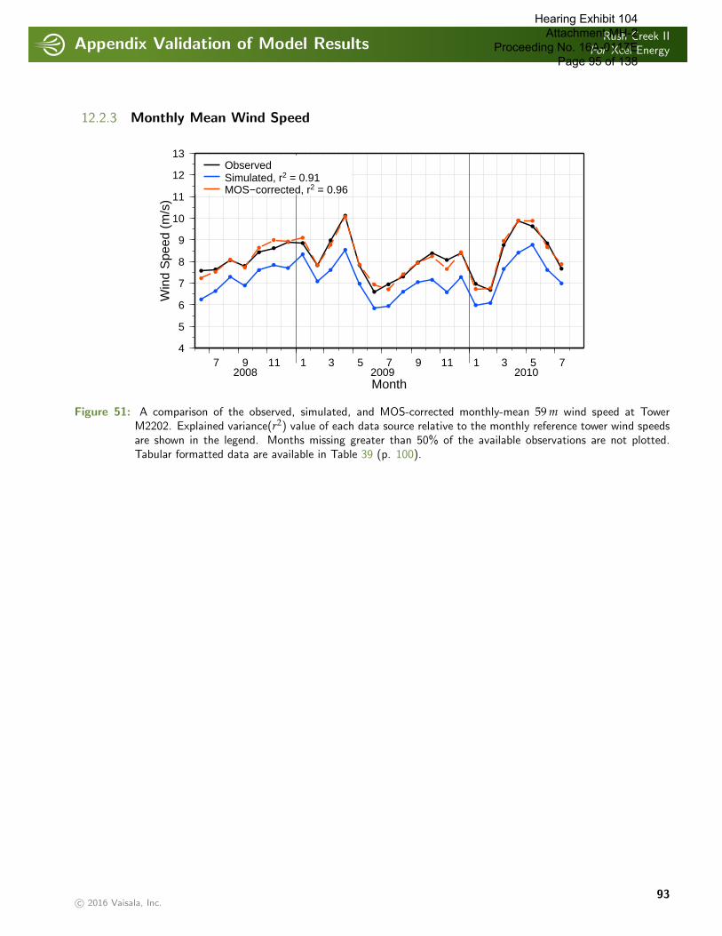
Appendix Validation of Model ResultsRush Creek II
For Xcel Energy
. . . . . . . . . . . . . . . . . . . . . . . . . . . . . . . . . . . . . . . . . . . . . . . . . . . . . . . . . . . . . . . . . . . . . . . . . . . . . . . . . . . . . . . . . . . . . . . . . . . . . . . . . . . . . . . . . .
12.2.3 Monthly Mean Wind Speed
7 9 11 1 3 5 7 9 11 1 3 5 7
Month2008 2009 2010
4
5
6
7
8
9
10
11
12
13W
ind
Spe
ed (
m/s
)ObservedSimulated, r2 = 0.91MOS−corrected, r2 = 0.96
Figure 51: A comparison of the observed, simulated, and MOS-corrected monthly-mean 59 m wind speed at TowerM2202. Explained variance(r2) value of each data source relative to the monthly reference tower wind speedsare shown in the legend. Months missing greater than 50% of the available observations are not plotted.Tabular formatted data are available in Table 39 (p. 100).
c© 2016 Vaisala, Inc.93
Hearing Exhibit 104 Attachment MH-2
Proceeding No. 16A-0117E Page 95 of 138
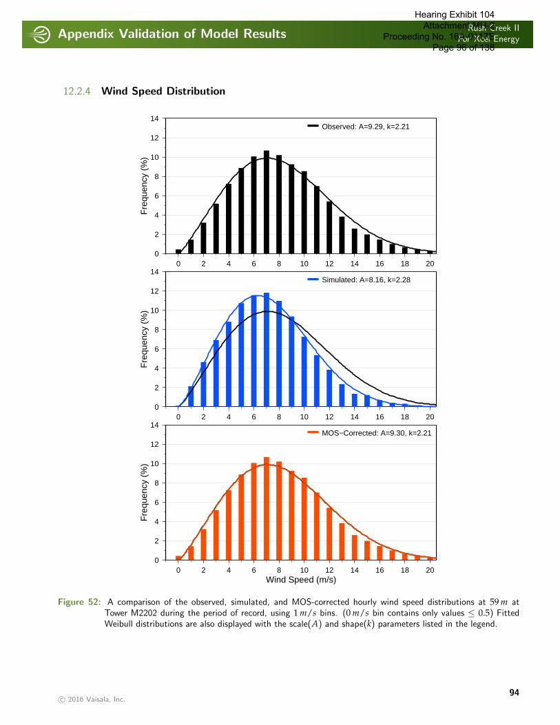
Appendix Validation of Model ResultsRush Creek II
For Xcel Energy
. . . . . . . . . . . . . . . . . . . . . . . . . . . . . . . . . . . . . . . . . . . . . . . . . . . . . . . . . . . . . . . . . . . . . . . . . . . . . . . . . . . . . . . . . . . . . . . . . . . . . . . . . . . . . . . . . .
12.2.4 Wind Speed Distribution
0 2 4 6 8 10 12 14 16 18 200
2
4
6
8
10
12
14
Fre
quen
cy (
%)
Observed: A=9.29, k=2.21
0 2 4 6 8 10 12 14 16 18 200
2
4
6
8
10
12
14
Fre
quen
cy (
%)
Simulated: A=8.16, k=2.28
0 2 4 6 8 10 12 14 16 18 20Wind Speed (m/s)
0
2
4
6
8
10
12
14
Fre
quen
cy (
%)
MOS−Corrected: A=9.30, k=2.21
Figure 52: A comparison of the observed, simulated, and MOS-corrected hourly wind speed distributions at 59 m atTower M2202 during the period of record, using 1 m/s bins. (0 m/s bin contains only values ≤ 0.5) FittedWeibull distributions are also displayed with the scale(A) and shape(k) parameters listed in the legend.
c© 2016 Vaisala, Inc.94
Hearing Exhibit 104 Attachment MH-2
Proceeding No. 16A-0117E Page 96 of 138

Appendix Validation of Model ResultsRush Creek II
For Xcel Energy
. . . . . . . . . . . . . . . . . . . . . . . . . . . . . . . . . . . . . . . . . . . . . . . . . . . . . . . . . . . . . . . . . . . . . . . . . . . . . . . . . . . . . . . . . . . . . . . . . . . . . . . . . . . . . . . . . .
12.2.5 Wind Direction Distribution
Observed
S 10 %
EW
N
S 10 %
EW
N
SW
NW
SE
NE
Simulated
S 10 %
EW
N
S 10 %
EW
N
SW
NW
SE
NE
MOS−Corrected
S 10 %
EW
N
S 10 %
EW
N
SW
NW
SE
NE
Figure 53: Wind roses at 57 m at Tower M2202 for observational data and simulated model data, averaged over theperiod of record (June, 2008–August, 2010). Directional bins are 22.5◦ wide, and the radial contour intervalis 10%. Tabular formatted data, including mean wind speed values and Weibull parameters for each winddirection sector, are available in Tables 42 and 43 (p. 105).
c© 2016 Vaisala, Inc.95
Hearing Exhibit 104 Attachment MH-2
Proceeding No. 16A-0117E Page 97 of 138
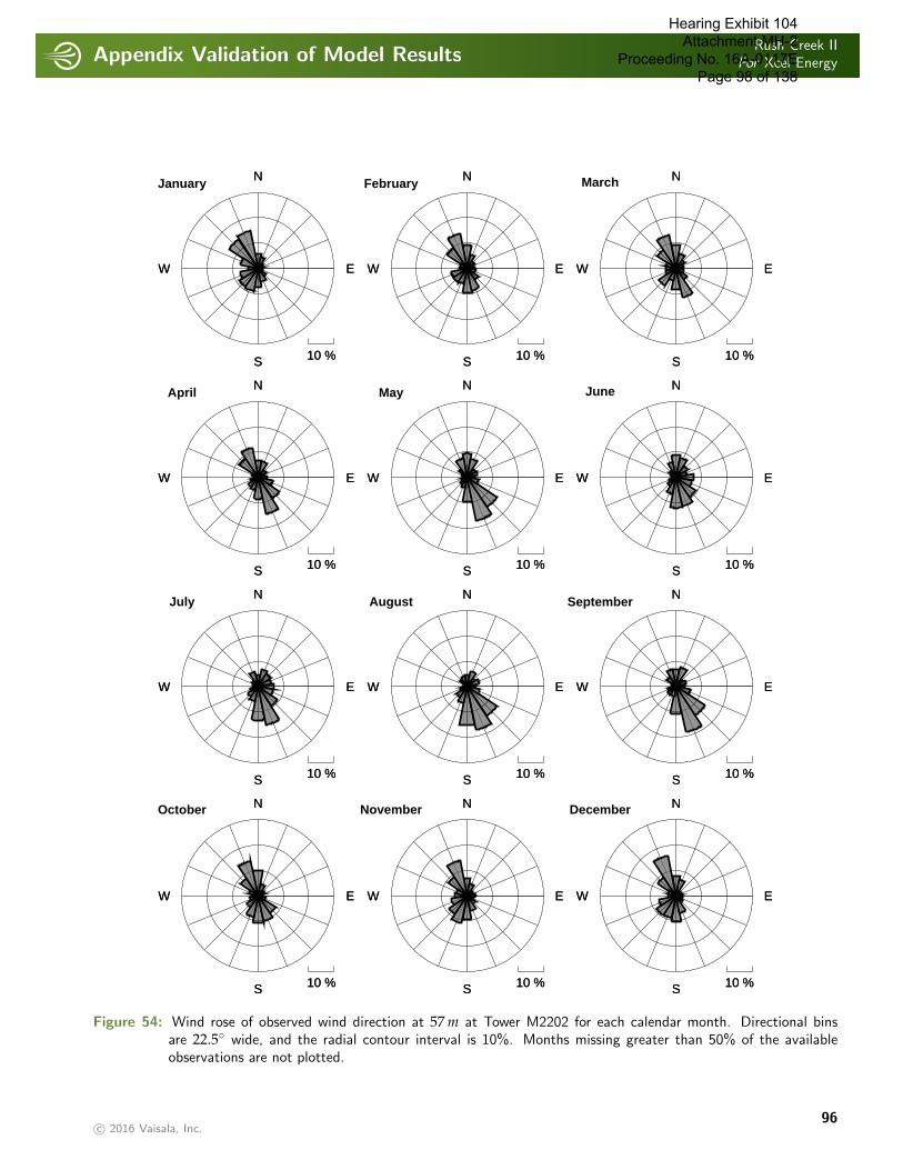
Appendix Validation of Model ResultsRush Creek II
For Xcel Energy
. . . . . . . . . . . . . . . . . . . . . . . . . . . . . . . . . . . . . . . . . . . . . . . . . . . . . . . . . . . . . . . . . . . . . . . . . . . . . . . . . . . . . . . . . . . . . . . . . . . . . . . . . . . . . . . . . .
S 10 %
EW
NOctober
S 10 %
EW
N
S 10 %
EW
NNovember
S 10 %
EW
N
S 10 %
EW
NDecember
S 10 %
EW
N
S 10 %
EW
NJuly
S 10 %
EW
N
S 10 %
EW
NAugust
S 10 %
EW
N
S 10 %
EW
NSeptember
S 10 %
EW
N
S 10 %
EW
NApril
S 10 %
EW
N
S 10 %
EW
NMay
S 10 %
EW
N
S 10 %
EW
NJune
S 10 %
EW
N
S 10 %
EW
NJanuary
S 10 %
EW
N
S 10 %
EW
NFebruary
S 10 %
EW
N
S 10 %
EW
NMarch
S 10 %
EW
N
Figure 54: Wind rose of observed wind direction at 57 m at Tower M2202 for each calendar month. Directional binsare 22.5◦ wide, and the radial contour interval is 10%. Months missing greater than 50% of the availableobservations are not plotted.
c© 2016 Vaisala, Inc.96
Hearing Exhibit 104 Attachment MH-2
Proceeding No. 16A-0117E Page 98 of 138
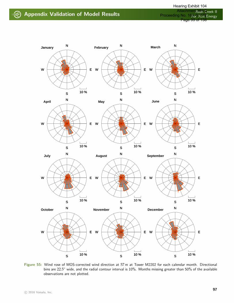
Appendix Validation of Model ResultsRush Creek II
For Xcel Energy
. . . . . . . . . . . . . . . . . . . . . . . . . . . . . . . . . . . . . . . . . . . . . . . . . . . . . . . . . . . . . . . . . . . . . . . . . . . . . . . . . . . . . . . . . . . . . . . . . . . . . . . . . . . . . . . . . .
S 10 %
EW
NOctober
S 10 %
EW
N
S 10 %
EW
NNovember
S 10 %
EW
N
S 10 %
EW
NDecember
S 10 %
EW
N
S 10 %
EW
NJuly
S 10 %
EW
N
S 10 %
EW
NAugust
S 10 %
EW
N
S 10 %
EW
NSeptember
S 10 %
EW
N
S 10 %
EW
NApril
S 10 %
EW
N
S 10 %
EW
NMay
S 10 %
EW
N
S 10 %
EW
NJune
S 10 %
EW
N
S 10 %
EW
NJanuary
S 10 %
EW
N
S 10 %
EW
NFebruary
S 10 %
EW
N
S 10 %
EW
NMarch
S 10 %
EW
N
Figure 55: Wind rose of MOS-corrected wind direction at 57 m at Tower M2202 for each calendar month. Directionalbins are 22.5◦ wide, and the radial contour interval is 10%. Months missing greater than 50% of the availableobservations are not plotted.
c© 2016 Vaisala, Inc.97
Hearing Exhibit 104 Attachment MH-2
Proceeding No. 16A-0117E Page 99 of 138

Appendix Validation of Model ResultsRush Creek II
For Xcel Energy
. . . . . . . . . . . . . . . . . . . . . . . . . . . . . . . . . . . . . . . . . . . . . . . . . . . . . . . . . . . . . . . . . . . . . . . . . . . . . . . . . . . . . . . . . . . . . . . . . . . . . . . . . . . . . . . . . .
12.2.6 Diurnal Variability of Wind Speed
0 4 8 12 16 20 24
Hour of Day (MST)
5
6
7
8
9
10
11
Win
d S
peed
(m
/s)
ObservedSimulatedMOS−corrected
Figure 56: A comparison of the diurnal cycle of observed, simulated, and MOS-corrected 59m wind speed at TowerM2202. Data are averaged over the period of record (June, 2008–August, 2010). Hours missing greater than15% of the available observations are not plotted. The horizontal axis is Mountain Standard Time (MST).Tabular formatted data are available in Figures 58 and 59 (p. 101 and 102).
c© 2016 Vaisala, Inc.98
Hearing Exhibit 104 Attachment MH-2
Proceeding No. 16A-0117E Page 100 of 138

Appendix Validation of Model ResultsRush Creek II
For Xcel Energy
. . . . . . . . . . . . . . . . . . . . . . . . . . . . . . . . . . . . . . . . . . . . . . . . . . . . . . . . . . . . . . . . . . . . . . . . . . . . . . . . . . . . . . . . . . . . . . . . . . . . . . . . . . . . . . . . . .
January
0 4 8 12 16 20 24
456789
101112
Win
d S
peed
(m
/s)
February
0 4 8 12 16 20 24
456789
101112
March
0 4 8 12 16 20 24
456789
101112
April
0 4 8 12 16 20 24
456789
101112
Win
d S
peed
(m
/s)
May
0 4 8 12 16 20 24
456789
101112
June
0 4 8 12 16 20 24
456789
101112
July
0 4 8 12 16 20 24
456789
101112
Win
d S
peed
(m
/s)
August
0 4 8 12 16 20 24
456789
101112
September
0 4 8 12 16 20 24
456789
101112
October
0 4 8 12 16 20 24Hour of Day (MST)
456789
101112
Win
d S
peed
(m
/s)
November
0 4 8 12 16 20 24Hour of Day (MST)
456789
101112
Observed Simulated MOS−corrected
December
0 4 8 12 16 20 24Hour of Day (MST)
456789
101112
Figure 57: A comparison of the diurnal cycle of observed, simulated, and MOS-corrected 59 m wind speed for eachcalendar month at Tower M2202. Hours missing greater than 50% of the available observations are notplotted. The horizontal axis is Mountain Standard Time (MST). Tabular formatted data available in Figures58 and 59 (p. 101 and 102).
c© 2016 Vaisala, Inc.99
Hearing Exhibit 104 Attachment MH-2
Proceeding No. 16A-0117E Page 101 of 138
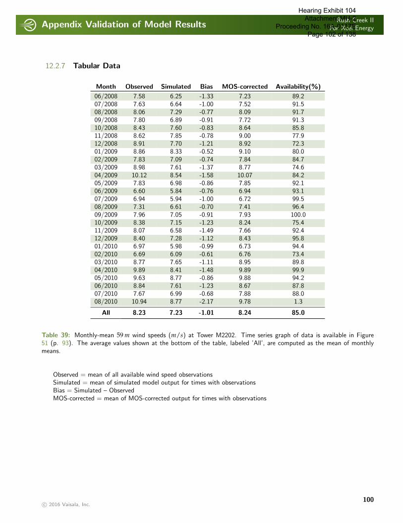
Appendix Validation of Model ResultsRush Creek II
For Xcel Energy
. . . . . . . . . . . . . . . . . . . . . . . . . . . . . . . . . . . . . . . . . . . . . . . . . . . . . . . . . . . . . . . . . . . . . . . . . . . . . . . . . . . . . . . . . . . . . . . . . . . . . . . . . . . . . . . . . .
12.2.7 Tabular Data
Month Observed Simulated Bias MOS-corrected Availability(%)
06/2008 7.58 6.25 -1.33 7.23 89.207/2008 7.63 6.64 -1.00 7.52 91.508/2008 8.06 7.29 -0.77 8.09 91.709/2008 7.80 6.89 -0.91 7.72 91.310/2008 8.43 7.60 -0.83 8.64 85.811/2008 8.62 7.85 -0.78 9.00 77.912/2008 8.91 7.70 -1.21 8.92 72.301/2009 8.86 8.33 -0.52 9.10 80.002/2009 7.83 7.09 -0.74 7.84 84.703/2009 8.98 7.61 -1.37 8.77 74.604/2009 10.12 8.54 -1.58 10.07 84.205/2009 7.83 6.98 -0.86 7.85 92.106/2009 6.60 5.84 -0.76 6.94 93.107/2009 6.94 5.94 -1.00 6.72 99.508/2009 7.31 6.61 -0.70 7.41 96.409/2009 7.96 7.05 -0.91 7.93 100.010/2009 8.38 7.15 -1.23 8.24 75.411/2009 8.07 6.58 -1.49 7.66 92.412/2009 8.40 7.28 -1.12 8.43 95.801/2010 6.97 5.98 -0.99 6.73 94.402/2010 6.69 6.09 -0.61 6.76 73.403/2010 8.77 7.65 -1.11 8.95 89.804/2010 9.89 8.41 -1.48 9.89 99.905/2010 9.63 8.77 -0.86 9.88 94.206/2010 8.84 7.61 -1.23 8.67 87.807/2010 7.67 6.99 -0.68 7.88 88.008/2010 10.94 8.77 -2.17 9.78 1.3
All 8.23 7.23 -1.01 8.24 85.0
Table 39: Monthly-mean 59 m wind speeds (m/s) at Tower M2202. Time series graph of data is available in Figure51 (p. 93). The average values shown at the bottom of the table, labeled ’All’, are computed as the mean of monthlymeans.
Observed = mean of all available wind speed observationsSimulated = mean of simulated model output for times with observationsBias = Simulated – ObservedMOS-corrected = mean of MOS-corrected output for times with observations
c© 2016 Vaisala, Inc.100
Hearing Exhibit 104 Attachment MH-2
Proceeding No. 16A-0117E Page 102 of 138
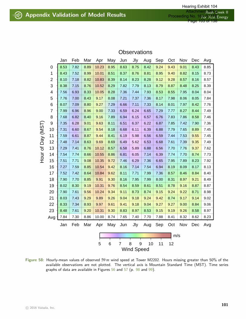
Appendix Validation of Model ResultsRush Creek II
For Xcel Energy
. . . . . . . . . . . . . . . . . . . . . . . . . . . . . . . . . . . . . . . . . . . . . . . . . . . . . . . . . . . . . . . . . . . . . . . . . . . . . . . . . . . . . . . . . . . . . . . . . . . . . . . . . . . . . . . . . .
Observations
Hou
r of
Day
(M
ST
)
012
34
567
89101112
1314
151617
1819202122
23
Avg
Jan
Jan
Feb
Feb
Mar
Mar
Apr
Apr
May
May
Jun
Jun
Jly
Jly
Aug
Aug
Sep
Sep
Oct
Oct
Nov
Nov
Dec
Dec
Avg
Avg
7.52
7.90
8.02
7.90
8.03
8.33
8.48
8.53
8.43
8.10
8.38
7.56
7.76
8.07
7.99
7.68
7.35
7.31
7.59
7.48
7.29
7.54
7.51
7.27
7.84
7.42
7.70
8.30
7.61
7.43
7.34
7.61
7.82
7.52
7.18
7.15
6.93
7.00
7.09
6.96
6.82
6.28
6.60
6.61
7.14
7.41
7.74
7.71
7.59
7.30
8.64
8.85
9.19
9.56
9.29
8.93
9.20
8.89
8.99
8.82
8.76
8.33
8.43
8.80
8.96
8.40
9.01
8.67
8.87
8.63
8.76
8.66
9.08
8.85
8.86
10.84
9.91
10.31
10.24
9.89
9.97
10.31
10.23
10.01
10.83
10.52
10.05
9.17
9.27
9.00
9.16
9.63
9.54
9.44
9.69
10.12
10.55
10.35
10.54
10.00
9.62
9.30
9.76
9.34
9.26
9.61
9.30
8.95
8.51
8.39
8.29
8.28
8.08
7.29
7.33
7.89
8.11
8.18
8.41
8.69
8.57
8.86
9.72
9.42
8.74
8.11
8.16
8.54
9.11
9.04
9.41
8.83
8.63
8.37
8.14
7.82
7.36
7.21
6.66
6.59
6.94
6.51
6.68
6.19
6.49
6.58
6.81
7.46
8.16
7.65
7.71
7.95
8.59
8.73
9.18
9.18
8.97
8.75
8.76
8.23
7.79
7.44
7.37
7.11
6.24
6.15
6.37
6.11
5.98
5.62
5.89
6.05
6.29
7.14
7.40
7.99
7.99
8.61
8.74
9.24
9.04
8.53
8.42
8.81
8.28
8.13
7.93
7.36
7.33
6.65
6.57
6.22
6.39
6.56
6.53
6.88
7.14
7.36
7.54
7.70
7.36
8.00
8.51
9.15
9.42
9.27
9.15
9.24
8.95
9.12
8.79
8.53
8.17
8.14
7.29
6.76
6.87
6.88
6.59
6.68
6.56
6.39
6.65
6.94
7.88
8.57
8.31
8.78
9.24
8.74
9.27
9.19
9.43
9.40
9.28
8.87
8.55
7.98
8.01
7.77
7.83
7.85
7.79
7.44
7.61
7.70
7.74
7.95
8.19
8.41
8.46
8.97
9.16
9.22
9.17
9.00
9.26
9.01
8.82
8.57
8.48
7.95
8.06
7.97
8.27
7.86
7.42
7.65
7.53
7.39
7.76
7.70
7.89
8.09
8.32
8.84
9.21
8.87
8.71
9.14
8.84
8.58
8.43
8.15
8.16
8.25
8.04
8.05
8.42
8.44
8.58
7.90
8.89
9.55
9.35
9.37
8.74
8.23
8.17
8.62
8.40
8.49
8.87
8.98
9.02
9.06
8.97
8.85
8.73
8.57
8.39
8.04
7.84
7.76
7.49
7.46
7.36
7.45
7.45
7.49
7.62
7.73
7.92
8.13
8.23
5 6 7 8 9 10 11 12Wind Speed
m/s
Figure 58: Hourly-mean values of observed 59 m wind speed at Tower M2202. Hours missing greater than 50% of theavailable observations are not plotted. The vertical axis is Mountain Standard Time (MST). Time seriesgraphs of data are available in Figures 56 and 57 (p. 98 and 99).
c© 2016 Vaisala, Inc.101
Hearing Exhibit 104 Attachment MH-2
Proceeding No. 16A-0117E Page 103 of 138

Appendix Validation of Model ResultsRush Creek II
For Xcel Energy
. . . . . . . . . . . . . . . . . . . . . . . . . . . . . . . . . . . . . . . . . . . . . . . . . . . . . . . . . . . . . . . . . . . . . . . . . . . . . . . . . . . . . . . . . . . . . . . . . . . . . . . . . . . . . . . . . .
MOS−Corrected
Hou
r of
Day
(M
ST
)
012
34
567
89
101112
1314
151617
1819202122
23
Avg
Jan
Jan
Feb
Feb
Mar
Mar
Apr
Apr
May
May
Jun
Jun
Jly
Jly
Aug
Aug
Sep
Sep
Oct
Oct
Nov
Nov
Dec
Dec
Avg
Avg
7.59
7.88
8.23
8.07
8.15
8.23
8.40
8.45
8.34
8.11
8.24
7.63
7.76
7.98
7.96
7.63
7.37
7.29
7.45
7.44
7.27
7.46
7.37
7.32
7.82
7.35
7.71
8.09
7.70
7.53
7.51
7.75
7.82
7.63
7.18
7.23
7.02
7.14
7.21
7.14
6.96
6.49
6.47
6.63
7.02
7.49
7.71
7.63
7.50
7.34
8.80
8.81
9.34
9.48
9.17
8.86
9.19
9.11
9.05
9.24
8.88
8.51
8.40
8.86
8.94
8.50
8.80
8.48
8.66
8.48
8.60
8.70
9.09
8.97
8.87
10.82
10.02
10.08
10.08
10.12
10.20
10.30
10.12
10.10
10.40
10.23
9.89
9.21
9.10
8.94
9.03
9.46
9.56
9.57
9.89
10.14
10.49
10.49
10.66
9.97
9.64
9.59
9.69
9.71
9.47
9.62
9.43
9.12
8.69
8.61
8.50
8.56
8.21
7.62
7.58
8.15
8.28
8.29
8.43
8.59
8.74
8.98
9.46
9.52
8.88
8.34
8.22
8.66
8.95
9.26
9.35
8.89
8.61
8.37
8.14
7.75
7.27
7.21
6.67
6.30
6.61
6.38
6.35
6.05
6.25
6.44
6.93
7.46
8.01
7.60
7.41
7.87
8.56
8.85
9.06
9.16
8.93
8.82
8.73
8.16
7.84
7.48
7.34
6.94
6.21
6.12
6.21
6.05
5.89
5.67
5.81
5.94
6.31
7.02
7.35
8.13
8.12
8.67
8.89
9.35
9.20
8.75
8.67
8.81
8.44
8.25
8.03
7.55
7.45
6.63
6.44
6.33
6.37
6.38
6.46
6.78
6.97
7.32
7.60
7.76
7.38
7.85
8.48
9.21
9.37
9.29
9.17
9.25
9.02
9.10
8.74
8.40
7.97
7.80
7.22
6.66
6.66
6.79
6.63
6.64
6.52
6.45
6.62
6.91
7.83
8.58
8.65
9.05
9.33
9.14
9.25
9.52
9.55
9.44
9.38
8.98
8.53
8.16
8.07
7.98
7.89
7.59
7.54
7.27
7.42
7.56
7.64
7.99
8.09
8.45
8.26
8.66
9.00
9.12
9.20
9.07
8.97
8.84
8.68
8.58
8.42
8.01
8.24
8.13
8.24
7.93
7.42
7.60
7.58
7.47
7.70
7.62
7.75
7.93
8.27
8.91
9.40
8.89
8.76
9.03
8.81
8.75
8.62
8.35
8.18
8.27
7.99
7.95
8.28
8.26
8.48
8.03
8.84
9.50
9.26
9.31
8.84
8.47
8.29
8.64
8.40
8.53
8.89
9.03
9.11
9.09
9.01
8.91
8.77
8.60
8.40
8.06
7.87
7.74
7.47
7.42
7.31
7.36
7.39
7.43
7.57
7.71
7.90
8.11
8.24
5 6 7 8 9 10 11 12Wind Speed
m/s
Figure 59: Hourly-mean values of MOS-corrected 59 m wind speed at Tower M2202. Hours missing greater than 50% ofthe available observations are not plotted. The vertical axis is Mountain Standard Time (MST). Time seriesgraphs of data are available in Figures 56 and 57 (p. 98 and 99).
c© 2016 Vaisala, Inc.102
Hearing Exhibit 104 Attachment MH-2
Proceeding No. 16A-0117E Page 104 of 138

Appendix Validation of Model ResultsRush Creek II
For Xcel Energy
. . . . . . . . . . . . . . . . . . . . . . . . . . . . . . . . . . . . . . . . . . . . . . . . . . . . . . . . . . . . . . . . . . . . . . . . . . . . . . . . . . . . . . . . . . . . . . . . . . . . . . . . . . . . . . . . . .
Win
dSpee
dN
NN
EN
EEN
EE
ESE
SE
SSE
SSSW
SW
WSW
WW
NW
NW
NN
WA
ll(m
/s)
0-
0.5
0.03
0.01
0.05
0.05
0.04
0.02
0.01
0.02
0.02
0.02
0.01
0.02
0.03
0.02
0.04
0.04
0.44
0.5
-1.
50.
100.
090.
130.
100.
100.
110.
070.
070.
110.
090.
030.
080.
110.
140.
050.
071.
431.
5-
2.5
0.24
0.19
0.26
0.21
0.23
0.23
0.12
0.21
0.17
0.14
0.09
0.14
0.20
0.20
0.26
0.29
3.20
2.5
-3.
50.
360.
390.
340.
380.
360.
330.
410.
360.
380.
210.
200.
270.
210.
260.
290.
395.
153.
5-
4.5
0.62
0.58
0.52
0.45
0.48
0.45
0.49
0.55
0.63
0.31
0.24
0.32
0.26
0.29
0.46
0.53
7.18
4.5
-5.
50.
620.
700.
500.
580.
520.
550.
690.
760.
750.
510.
250.
330.
320.
330.
600.
798.
825.
5-
6.5
0.73
0.77
0.48
0.64
0.71
0.55
0.79
0.89
0.92
0.64
0.32
0.30
0.27
0.42
0.65
0.87
9.97
6.5
-7.
50.
840.
800.
290.
560.
450.
551.
081.
141.
160.
660.
300.
480.
360.
380.
780.
7910
.63
7.5
-8.
50.
820.
760.
410.
300.
420.
561.
011.
061.
150.
630.
330.
410.
300.
290.
720.
9810
.16
8.5
-9.
50.
730.
700.
170.
200.
260.
510.
911.
181.
340.
490.
350.
320.
230.
250.
630.
949.
219.
5-
10.5
0.73
0.44
0.13
0.12
0.24
0.36
0.93
1.22
1.15
0.48
0.33
0.32
0.17
0.27
0.72
0.91
8.50
10.5
-11
.50.
580.
290.
050.
130.
110.
270.
831.
341.
010.
390.
150.
230.
160.
160.
420.
846.
9611
.5-
12.5
0.43
0.13
0.03
0.04
0.03
0.10
0.56
1.37
1.00
0.21
0.17
0.10
0.05
0.12
0.41
0.65
5.38
12.5
-13
.50.
440.
110.
030.
020.
060.
050.
441.
000.
490.
210.
080.
060.
040.
040.
240.
513.
8113
.5-
14.5
0.19
0.05
0.01
0.02
0.02
0.05
0.31
0.67
0.36
0.07
0.06
0.02
0.04
0.04
0.21
0.46
2.57
14.5
-15
.50.
150.
030.
020.
010.
010.
020.
290.
520.
260.
070.
030.
040.
010.
010.
170.
331.
9715
.5-
16.5
0.12
0.02
0.00
0.01
0.01
0.02
0.14
0.33
0.14
0.03
0.05
0.00
0.01
0.02
0.13
0.44
1.45
16.5
-17
.50.
040.
010.
000.
000.
000.
020.
170.
190.
130.
060.
040.
010.
010.
010.
040.
291.
0017
.5-
18.5
0.04
0.00
0.01
0.00
0.01
0.01
0.07
0.11
0.07
0.02
0.01
0.01
0.01
0.01
0.07
0.21
0.64
18.5
-19
.50.
010.
000.
000.
000.
000.
000.
020.
050.
040.
000.
030.
000.
000.
020.
050.
220.
4419
.5-
20.5
0.02
0.00
0.00
0.00
0.01
0.00
0.02
0.04
0.01
0.01
0.02
0.01
0.00
0.00
0.05
0.13
0.31
20.5
-21
.50.
000.
000.
000.
000.
010.
000.
000.
050.
010.
000.
010.
010.
000.
000.
060.
130.
2721
.5-
22.5
0.00
0.00
0.00
0.00
0.00
0.00
0.01
0.05
0.02
0.00
0.00
0.00
0.00
0.00
0.02
0.10
0.19
22.5
-23
.50.
000.
000.
000.
000.
000.
000.
000.
010.
010.
000.
010.
000.
000.
000.
010.
040.
0823
.5-
24.5
0.00
0.00
0.00
0.00
0.00
0.00
0.00
0.01
0.02
0.00
0.01
0.00
0.00
0.00
0.02
0.03
0.08
>24
.50.
000.
000.
000.
000.
000.
000.
000.
010.
010.
000.
000.
000.
000.
000.
000.
020.
04
Table
40:
Distr
ibution
ofob
serv
ed59
mw
ind
spee
dby
direc
tion
atTow
erM
2202
.H
isto
gram
ofdat
ais
avai
lable
inFig
ure
52(p
.94
).
c© 2016 Vaisala, Inc.103
Hearing Exhibit 104 Attachment MH-2
Proceeding No. 16A-0117E Page 105 of 138
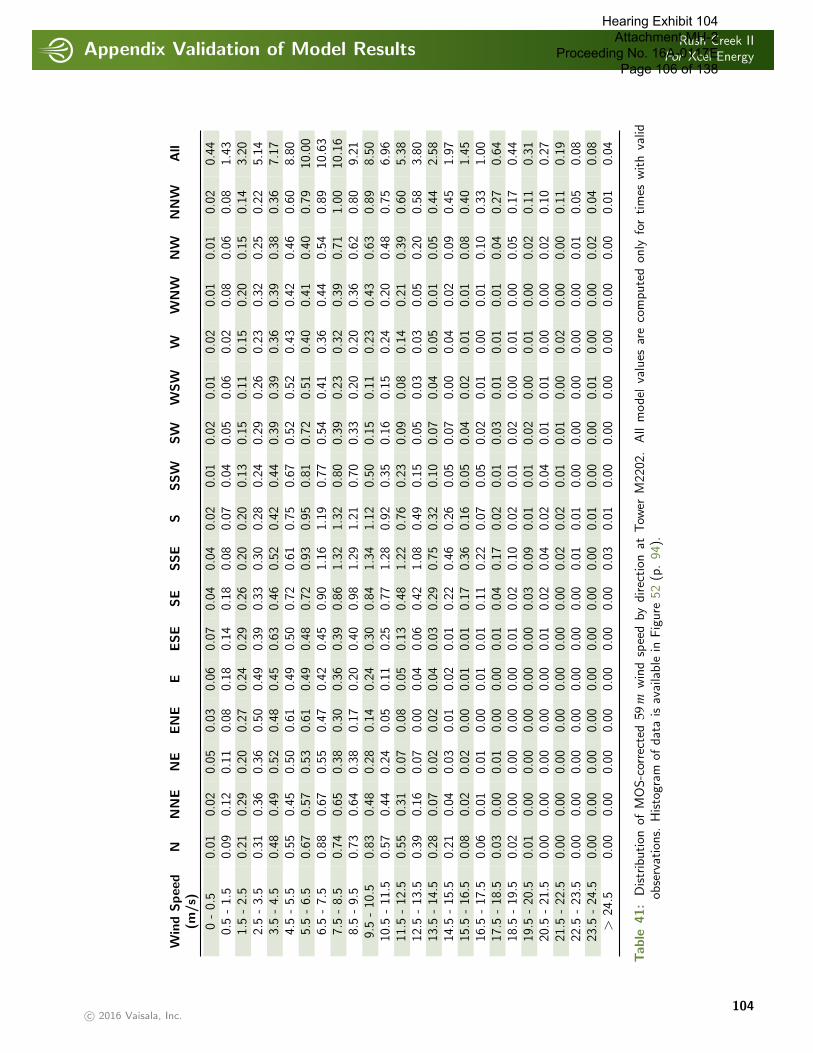
Appendix Validation of Model ResultsRush Creek II
For Xcel Energy
. . . . . . . . . . . . . . . . . . . . . . . . . . . . . . . . . . . . . . . . . . . . . . . . . . . . . . . . . . . . . . . . . . . . . . . . . . . . . . . . . . . . . . . . . . . . . . . . . . . . . . . . . . . . . . . . . .
Win
dSpee
dN
NN
EN
EEN
EE
ESE
SE
SSE
SSSW
SW
WSW
WW
NW
NW
NN
WA
ll(m
/s)
0-
0.5
0.01
0.02
0.05
0.03
0.06
0.07
0.04
0.04
0.02
0.01
0.02
0.01
0.02
0.01
0.01
0.02
0.44
0.5
-1.
50.
090.
120.
110.
080.
180.
140.
180.
080.
070.
040.
050.
060.
020.
080.
060.
081.
431.
5-
2.5
0.21
0.29
0.20
0.27
0.24
0.29
0.26
0.20
0.20
0.13
0.15
0.11
0.15
0.20
0.15
0.14
3.20
2.5
-3.
50.
310.
360.
360.
500.
490.
390.
330.
300.
280.
240.
290.
260.
230.
320.
250.
225.
143.
5-
4.5
0.48
0.49
0.52
0.48
0.45
0.63
0.46
0.52
0.42
0.44
0.39
0.39
0.36
0.39
0.38
0.36
7.17
4.5
-5.
50.
550.
450.
500.
610.
490.
500.
720.
610.
750.
670.
520.
520.
430.
420.
460.
608.
805.
5-
6.5
0.67
0.57
0.53
0.61
0.49
0.48
0.72
0.93
0.95
0.81
0.72
0.51
0.40
0.41
0.40
0.79
10.0
06.
5-
7.5
0.88
0.67
0.55
0.47
0.42
0.45
0.90
1.16
1.19
0.77
0.54
0.41
0.36
0.44
0.54
0.89
10.6
37.
5-
8.5
0.74
0.65
0.38
0.30
0.36
0.39
0.86
1.32
1.32
0.80
0.39
0.23
0.32
0.39
0.71
1.00
10.1
68.
5-
9.5
0.73
0.64
0.38
0.17
0.20
0.40
0.98
1.29
1.21
0.70
0.33
0.20
0.20
0.36
0.62
0.80
9.21
9.5
-10
.50.
830.
480.
280.
140.
240.
300.
841.
341.
120.
500.
150.
110.
230.
430.
630.
898.
5010
.5-
11.5
0.57
0.44
0.24
0.05
0.11
0.25
0.77
1.28
0.92
0.35
0.16
0.15
0.24
0.20
0.48
0.75
6.96
11.5
-12
.50.
550.
310.
070.
080.
050.
130.
481.
220.
760.
230.
090.
080.
140.
210.
390.
605.
3812
.5-
13.5
0.39
0.16
0.07
0.00
0.04
0.06
0.42
1.08
0.49
0.15
0.05
0.03
0.03
0.05
0.20
0.58
3.80
13.5
-14
.50.
280.
070.
020.
020.
040.
030.
290.
750.
320.
100.
070.
040.
050.
010.
050.
442.
5814
.5-
15.5
0.21
0.04
0.03
0.01
0.02
0.01
0.22
0.46
0.26
0.05
0.07
0.00
0.04
0.02
0.09
0.45
1.97
15.5
-16
.50.
080.
020.
020.
000.
010.
010.
170.
360.
160.
050.
040.
020.
010.
010.
080.
401.
4516
.5-
17.5
0.06
0.01
0.01
0.00
0.01
0.01
0.11
0.22
0.07
0.05
0.02
0.01
0.00
0.01
0.10
0.33
1.00
17.5
-18
.50.
030.
000.
010.
000.
000.
010.
040.
170.
020.
010.
030.
010.
010.
010.
040.
270.
6418
.5-
19.5
0.02
0.00
0.00
0.00
0.00
0.01
0.02
0.10
0.02
0.01
0.02
0.00
0.01
0.00
0.05
0.17
0.44
19.5
-20
.50.
010.
000.
000.
000.
000.
000.
030.
090.
010.
010.
020.
000.
010.
000.
020.
110.
3120
.5-
21.5
0.00
0.00
0.00
0.00
0.00
0.01
0.02
0.04
0.02
0.04
0.01
0.01
0.00
0.00
0.02
0.10
0.27
21.5
-22
.50.
000.
000.
000.
000.
000.
000.
000.
020.
020.
010.
010.
000.
020.
000.
000.
110.
1922
.5-
23.5
0.00
0.00
0.00
0.00
0.00
0.00
0.00
0.01
0.01
0.00
0.00
0.00
0.00
0.00
0.01
0.05
0.08
23.5
-24
.50.
000.
000.
000.
000.
000.
000.
000.
000.
010.
000.
000.
010.
000.
000.
020.
040.
08>
24.5
0.00
0.00
0.00
0.00
0.00
0.00
0.00
0.03
0.01
0.00
0.00
0.00
0.00
0.00
0.00
0.01
0.04
Table
41:
Distr
ibution
ofM
OS-c
orre
cted
59m
win
dsp
eed
bydirec
tion
atTow
erM
2202
.A
llm
odel
valu
esar
eco
mpute
don
lyfo
rtim
esw
ith
valid
obse
rvat
ions.
Histo
gram
ofdat
ais
avai
lable
inFig
ure
52(p
.94
).
c© 2016 Vaisala, Inc.104
Hearing Exhibit 104 Attachment MH-2
Proceeding No. 16A-0117E Page 106 of 138
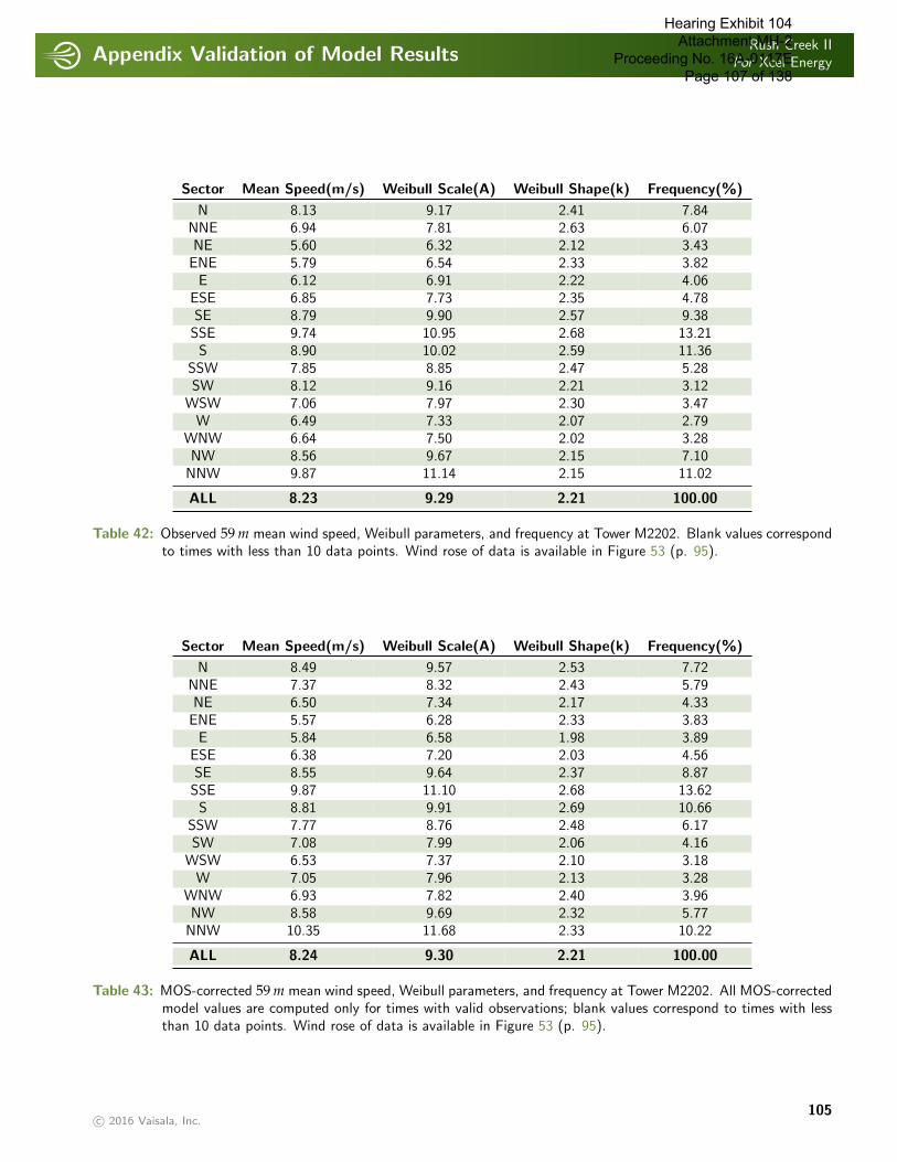
Appendix Validation of Model ResultsRush Creek II
For Xcel Energy
. . . . . . . . . . . . . . . . . . . . . . . . . . . . . . . . . . . . . . . . . . . . . . . . . . . . . . . . . . . . . . . . . . . . . . . . . . . . . . . . . . . . . . . . . . . . . . . . . . . . . . . . . . . . . . . . . .
Sector Mean Speed(m/s) Weibull Scale(A) Weibull Shape(k) Frequency(%)
N 8.13 9.17 2.41 7.84NNE 6.94 7.81 2.63 6.07NE 5.60 6.32 2.12 3.43ENE 5.79 6.54 2.33 3.82E 6.12 6.91 2.22 4.06
ESE 6.85 7.73 2.35 4.78SE 8.79 9.90 2.57 9.38SSE 9.74 10.95 2.68 13.21S 8.90 10.02 2.59 11.36
SSW 7.85 8.85 2.47 5.28SW 8.12 9.16 2.21 3.12
WSW 7.06 7.97 2.30 3.47W 6.49 7.33 2.07 2.79
WNW 6.64 7.50 2.02 3.28NW 8.56 9.67 2.15 7.10
NNW 9.87 11.14 2.15 11.02
ALL 8.23 9.29 2.21 100.00
Table 42: Observed 59 m mean wind speed, Weibull parameters, and frequency at Tower M2202. Blank values correspondto times with less than 10 data points. Wind rose of data is available in Figure 53 (p. 95).
Sector Mean Speed(m/s) Weibull Scale(A) Weibull Shape(k) Frequency(%)
N 8.49 9.57 2.53 7.72NNE 7.37 8.32 2.43 5.79NE 6.50 7.34 2.17 4.33ENE 5.57 6.28 2.33 3.83E 5.84 6.58 1.98 3.89
ESE 6.38 7.20 2.03 4.56SE 8.55 9.64 2.37 8.87SSE 9.87 11.10 2.68 13.62S 8.81 9.91 2.69 10.66
SSW 7.77 8.76 2.48 6.17SW 7.08 7.99 2.06 4.16
WSW 6.53 7.37 2.10 3.18W 7.05 7.96 2.13 3.28
WNW 6.93 7.82 2.40 3.96NW 8.58 9.69 2.32 5.77
NNW 10.35 11.68 2.33 10.22
ALL 8.24 9.30 2.21 100.00
Table 43: MOS-corrected 59 m mean wind speed, Weibull parameters, and frequency at Tower M2202. All MOS-correctedmodel values are computed only for times with valid observations; blank values correspond to times with lessthan 10 data points. Wind rose of data is available in Figure 53 (p. 95).
c© 2016 Vaisala, Inc.105
Hearing Exhibit 104 Attachment MH-2
Proceeding No. 16A-0117E Page 107 of 138

Appendix Validation of Model ResultsRush Creek II
For Xcel Energy
. . . . . . . . . . . . . . . . . . . . . . . . . . . . . . . . . . . . . . . . . . . . . . . . . . . . . . . . . . . . . . . . . . . . . . . . . . . . . . . . . . . . . . . . . . . . . . . . . . . . . . . . . . . . . . . . . .
12.3 Validation of Model Results at Tower M2311
This section examines the quality of the NWP simulations used at a single point within the study area. For this section,the observations were taken at Tower M2311 (latitude 39.08518, longitude -103.21049).
The average observed wind speed (for all valid observational times) at 60.0 m during the 32 months of the period of record(October, 2010 to May, 2013) is 8.53 m/s with an hourly standard deviation of 3.91 m/s at Tower M2311. This comparesto a modeled 60 m wind speed of 7.32 m/s with a 3.54 m/s standard deviation for these same times.
Based on a comparison of the NWP model output with observations from each of the meteorological towers for whichdata were provided, Model Output Statistics (MOS) was constructed. MOS uses a multilinear regression model designedto remove the bias and adjust the variance of the raw NWP simulated wind speed and direction. Applying this statisticalmodel to the simulated data at Tower M2311 results in a MOS-corrected mean value of 8.54 m/s and an hourly standarddeviation of 3.91 m/s.
This section presents a comparison of the simulated winds with the observations at the reference tower (Tower M2311).The focus of the verification is on the model’s ability to reproduce the observed variability of the wind resource at daily andmonthly time scales, while preserving the distribution of hourly wind speeds and the diurnal characteristics of the wind.
c© 2016 Vaisala, Inc.106
Hearing Exhibit 104 Attachment MH-2
Proceeding No. 16A-0117E Page 108 of 138

Appendix Validation of Model ResultsRush Creek II
For Xcel Energy
. . . . . . . . . . . . . . . . . . . . . . . . . . . . . . . . . . . . . . . . . . . . . . . . . . . . . . . . . . . . . . . . . . . . . . . . . . . . . . . . . . . . . . . . . . . . . . . . . . . . . . . . . . . . . . . . . .
12.3.1 Observational Data
Approximately 32 months of wind speed data at 60.0 meters and wind direction data at 58.0 meters (October, 2010 toMay, 2013) from a meteorological tower (Tower M2311) at Rush Creek II were used in this analysis. This tower will bereferred to as the reference tower throughout this section. The data at 60 m were used to assess the quality of the modelsimulations at 60 m.
It should be noted that meteorological observations provided to 3TIER are not allowed to influence the raw model simu-lations.
12.3.2 Model Validation Statistics
Table 44 presents some basic statistical measures of the model performance relative to the measured winds at the referencetower during the observational period. Also shown are values (labeled “MOS-corrected”) for model data with the statisticalmodel applied. For reference, the correlation of the reference tower data to itself is perfect and hence the explained variance(r2) value is 1.0.
The observed and modeled winds in this section represent the mean of all times during the month for which a valid windspeed or direction observation was available. Therefore they should not be interpreted as estimates of the true winds atthe site, but rather a verification of the model’s ability to reproduce the available observations. Any month or hour missinggreater than 50% of the available observations is omitted from the following figures, tables, and statistics.
Comparison Value
Correlation of monthly-mean simulated wind speed to observed 0.95RMS error of monthly-mean simulated wind speed 1.25 m/sCorrelation of monthly-mean MOS-corrected wind speed to observed 0.98RMS error of monthly-mean MOS-corrected wind speed 0.13 m/s
Correlation of daily-mean simulated wind speed to observed 0.89RMS error of daily-mean simulated wind speed 1.69 m/sCorrelation of daily-mean MOS-corrected wind speed to observed 0.90RMS error of daily-mean MOS-corrected wind speed 1.18 m/s
Table 44: Correlation and root mean square (RMS) error statistics of modeled wind speeds.
c© 2016 Vaisala, Inc.107
Hearing Exhibit 104 Attachment MH-2
Proceeding No. 16A-0117E Page 109 of 138
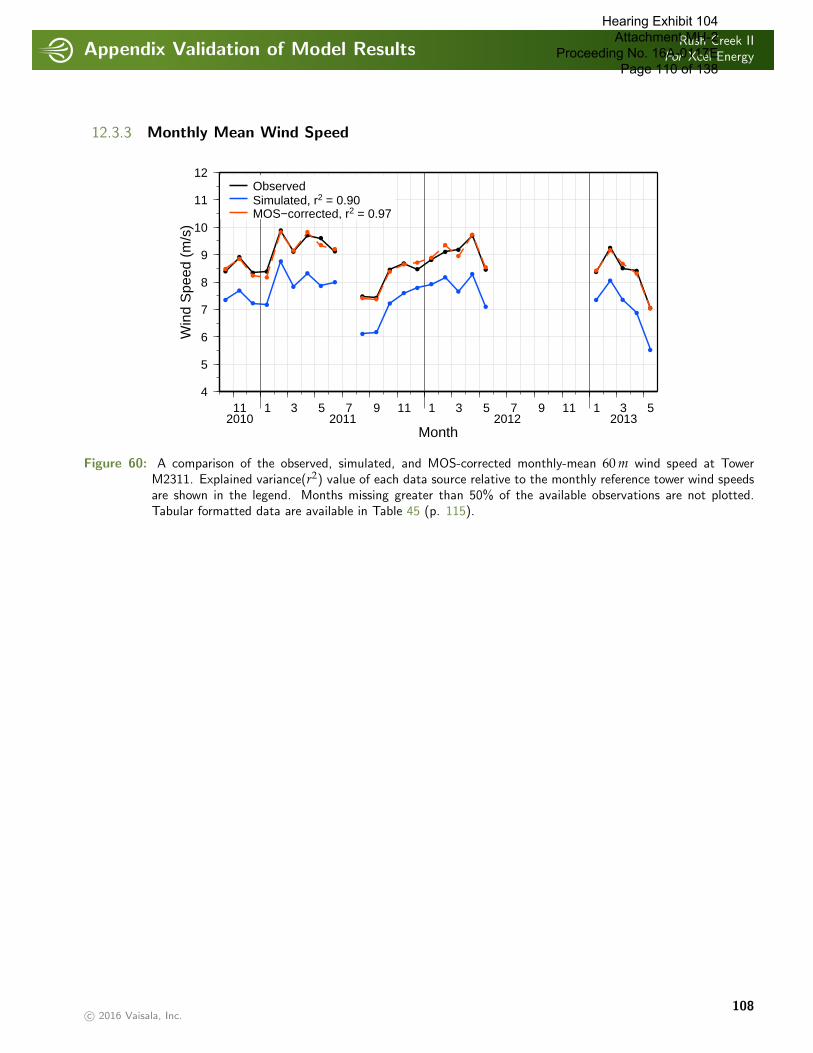
Appendix Validation of Model ResultsRush Creek II
For Xcel Energy
. . . . . . . . . . . . . . . . . . . . . . . . . . . . . . . . . . . . . . . . . . . . . . . . . . . . . . . . . . . . . . . . . . . . . . . . . . . . . . . . . . . . . . . . . . . . . . . . . . . . . . . . . . . . . . . . . .
12.3.3 Monthly Mean Wind Speed
11 1 3 5 7 9 11 1 3 5 7 9 11 1 3 5
Month2010 2011 2012 2013
4
5
6
7
8
9
10
11
12W
ind
Spe
ed (
m/s
)ObservedSimulated, r2 = 0.90MOS−corrected, r2 = 0.97
Figure 60: A comparison of the observed, simulated, and MOS-corrected monthly-mean 60 m wind speed at TowerM2311. Explained variance(r2) value of each data source relative to the monthly reference tower wind speedsare shown in the legend. Months missing greater than 50% of the available observations are not plotted.Tabular formatted data are available in Table 45 (p. 115).
c© 2016 Vaisala, Inc.108
Hearing Exhibit 104 Attachment MH-2
Proceeding No. 16A-0117E Page 110 of 138
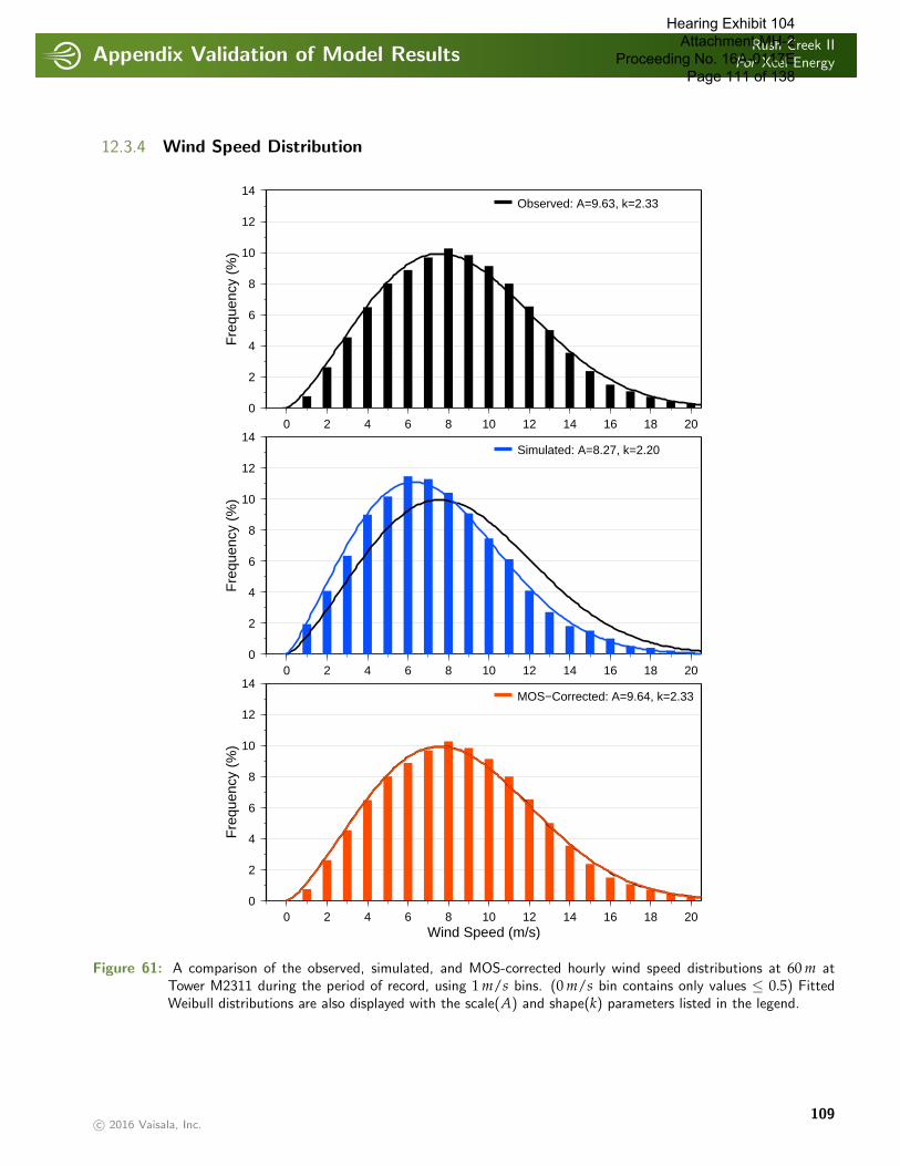
Appendix Validation of Model ResultsRush Creek II
For Xcel Energy
. . . . . . . . . . . . . . . . . . . . . . . . . . . . . . . . . . . . . . . . . . . . . . . . . . . . . . . . . . . . . . . . . . . . . . . . . . . . . . . . . . . . . . . . . . . . . . . . . . . . . . . . . . . . . . . . . .
12.3.4 Wind Speed Distribution
0 2 4 6 8 10 12 14 16 18 200
2
4
6
8
10
12
14
Fre
quen
cy (
%)
Observed: A=9.63, k=2.33
0 2 4 6 8 10 12 14 16 18 200
2
4
6
8
10
12
14
Fre
quen
cy (
%)
Simulated: A=8.27, k=2.20
0 2 4 6 8 10 12 14 16 18 20Wind Speed (m/s)
0
2
4
6
8
10
12
14
Fre
quen
cy (
%)
MOS−Corrected: A=9.64, k=2.33
Figure 61: A comparison of the observed, simulated, and MOS-corrected hourly wind speed distributions at 60 m atTower M2311 during the period of record, using 1 m/s bins. (0 m/s bin contains only values ≤ 0.5) FittedWeibull distributions are also displayed with the scale(A) and shape(k) parameters listed in the legend.
c© 2016 Vaisala, Inc.109
Hearing Exhibit 104 Attachment MH-2
Proceeding No. 16A-0117E Page 111 of 138
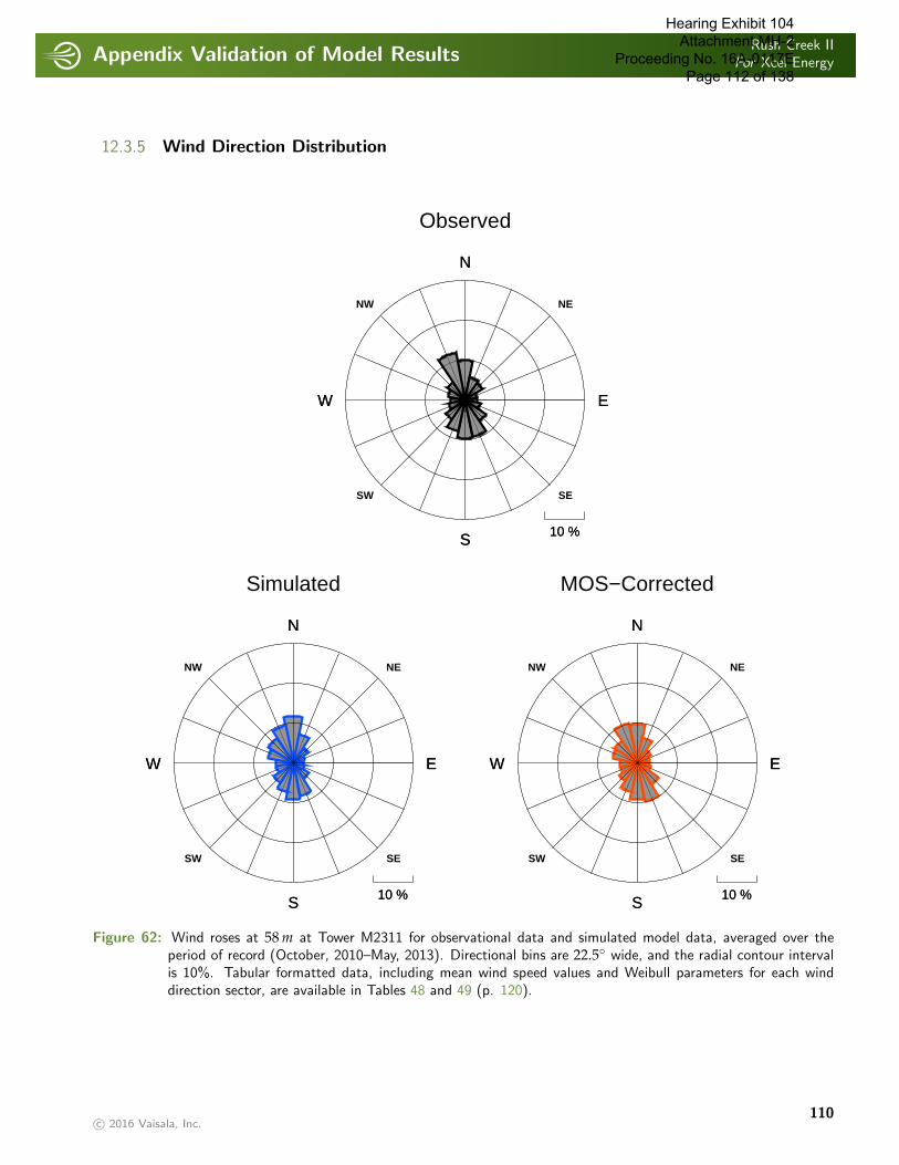
Appendix Validation of Model ResultsRush Creek II
For Xcel Energy
. . . . . . . . . . . . . . . . . . . . . . . . . . . . . . . . . . . . . . . . . . . . . . . . . . . . . . . . . . . . . . . . . . . . . . . . . . . . . . . . . . . . . . . . . . . . . . . . . . . . . . . . . . . . . . . . . .
12.3.5 Wind Direction Distribution
Observed
S 10 %
EW
N
S 10 %
EW
N
SW
NW
SE
NE
Simulated
S 10 %
EW
N
S 10 %
EW
N
SW
NW
SE
NE
MOS−Corrected
S 10 %
EW
N
S 10 %
EW
N
SW
NW
SE
NE
Figure 62: Wind roses at 58 m at Tower M2311 for observational data and simulated model data, averaged over theperiod of record (October, 2010–May, 2013). Directional bins are 22.5◦ wide, and the radial contour intervalis 10%. Tabular formatted data, including mean wind speed values and Weibull parameters for each winddirection sector, are available in Tables 48 and 49 (p. 120).
c© 2016 Vaisala, Inc.110
Hearing Exhibit 104 Attachment MH-2
Proceeding No. 16A-0117E Page 112 of 138
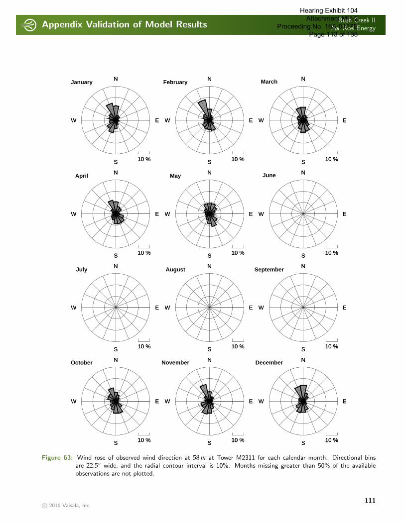
Appendix Validation of Model ResultsRush Creek II
For Xcel Energy
. . . . . . . . . . . . . . . . . . . . . . . . . . . . . . . . . . . . . . . . . . . . . . . . . . . . . . . . . . . . . . . . . . . . . . . . . . . . . . . . . . . . . . . . . . . . . . . . . . . . . . . . . . . . . . . . . .
S 10 %
EW
NOctober
S 10 %
EW
N
S 10 %
EW
NNovember
S 10 %
EW
N
S 10 %
EW
NDecember
S 10 %
EW
N
S 10 %
EW
NJuly
S 10 %
EW
N
S 10 %
EW
NAugust
S 10 %
EW
N
S 10 %
EW
NSeptember
S 10 %
EW
N
S 10 %
EW
NApril
S 10 %
EW
N
S 10 %
EW
NMay
S 10 %
EW
N
S 10 %
EW
NJune
S 10 %
EW
N
S 10 %
EW
NJanuary
S 10 %
EW
N
S 10 %
EW
NFebruary
S 10 %
EW
N
S 10 %
EW
NMarch
S 10 %
EW
N
Figure 63: Wind rose of observed wind direction at 58 m at Tower M2311 for each calendar month. Directional binsare 22.5◦ wide, and the radial contour interval is 10%. Months missing greater than 50% of the availableobservations are not plotted.
c© 2016 Vaisala, Inc.111
Hearing Exhibit 104 Attachment MH-2
Proceeding No. 16A-0117E Page 113 of 138
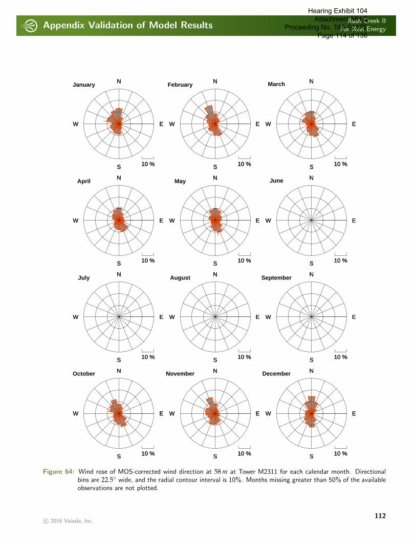
Appendix Validation of Model ResultsRush Creek II
For Xcel Energy
. . . . . . . . . . . . . . . . . . . . . . . . . . . . . . . . . . . . . . . . . . . . . . . . . . . . . . . . . . . . . . . . . . . . . . . . . . . . . . . . . . . . . . . . . . . . . . . . . . . . . . . . . . . . . . . . . .
S 10 %
EW
NOctober
S 10 %
EW
N
S 10 %
EW
NNovember
S 10 %
EW
N
S 10 %
EW
NDecember
S 10 %
EW
N
S 10 %
EW
NJuly
S 10 %
EW
N
S 10 %
EW
NAugust
S 10 %
EW
N
S 10 %
EW
NSeptember
S 10 %
EW
N
S 10 %
EW
NApril
S 10 %
EW
N
S 10 %
EW
NMay
S 10 %
EW
N
S 10 %
EW
NJune
S 10 %
EW
N
S 10 %
EW
NJanuary
S 10 %
EW
N
S 10 %
EW
NFebruary
S 10 %
EW
N
S 10 %
EW
NMarch
S 10 %
EW
N
Figure 64: Wind rose of MOS-corrected wind direction at 58 m at Tower M2311 for each calendar month. Directionalbins are 22.5◦ wide, and the radial contour interval is 10%. Months missing greater than 50% of the availableobservations are not plotted.
c© 2016 Vaisala, Inc.112
Hearing Exhibit 104 Attachment MH-2
Proceeding No. 16A-0117E Page 114 of 138
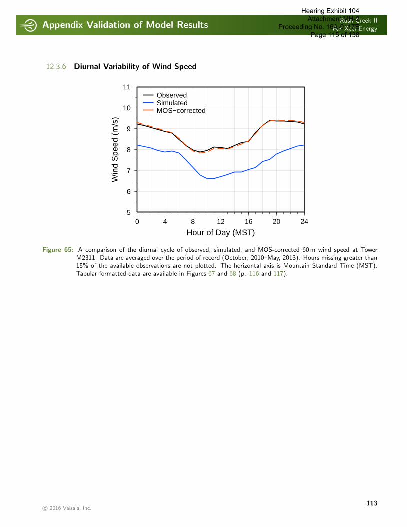
Appendix Validation of Model ResultsRush Creek II
For Xcel Energy
. . . . . . . . . . . . . . . . . . . . . . . . . . . . . . . . . . . . . . . . . . . . . . . . . . . . . . . . . . . . . . . . . . . . . . . . . . . . . . . . . . . . . . . . . . . . . . . . . . . . . . . . . . . . . . . . . .
12.3.6 Diurnal Variability of Wind Speed
0 4 8 12 16 20 24
Hour of Day (MST)
5
6
7
8
9
10
11
Win
d S
peed
(m
/s)
ObservedSimulatedMOS−corrected
Figure 65: A comparison of the diurnal cycle of observed, simulated, and MOS-corrected 60m wind speed at TowerM2311. Data are averaged over the period of record (October, 2010–May, 2013). Hours missing greater than15% of the available observations are not plotted. The horizontal axis is Mountain Standard Time (MST).Tabular formatted data are available in Figures 67 and 68 (p. 116 and 117).
c© 2016 Vaisala, Inc.113
Hearing Exhibit 104 Attachment MH-2
Proceeding No. 16A-0117E Page 115 of 138
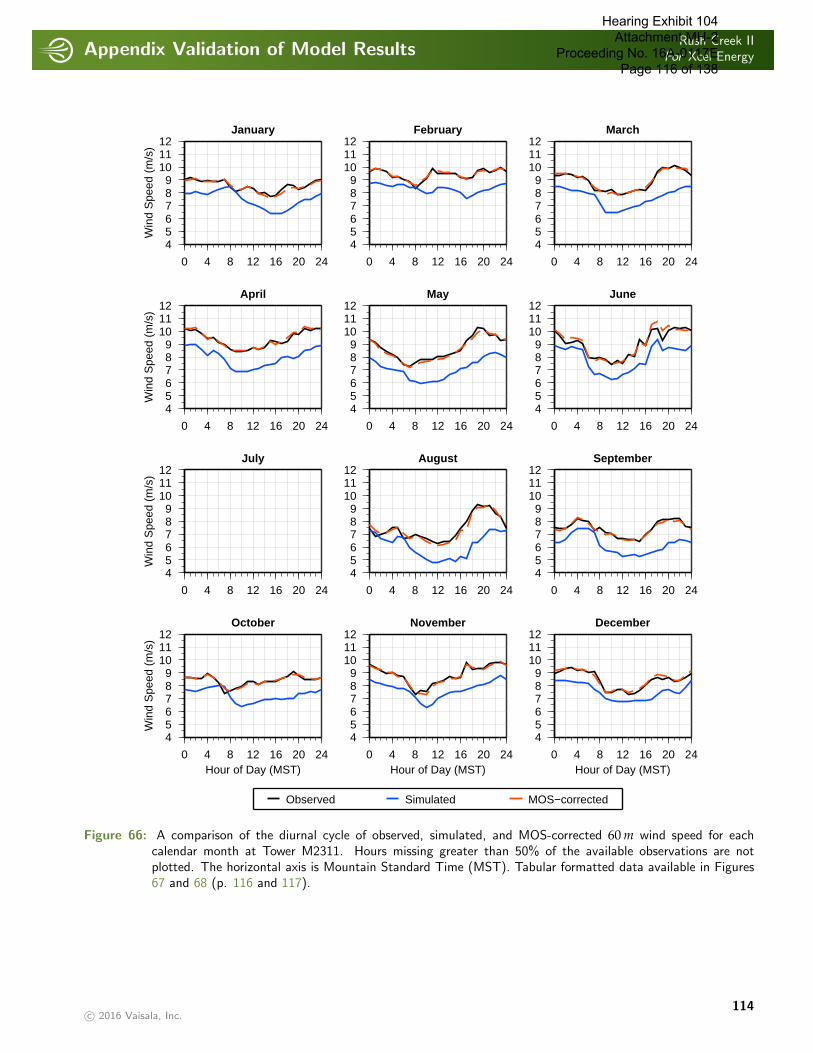
Appendix Validation of Model ResultsRush Creek II
For Xcel Energy
. . . . . . . . . . . . . . . . . . . . . . . . . . . . . . . . . . . . . . . . . . . . . . . . . . . . . . . . . . . . . . . . . . . . . . . . . . . . . . . . . . . . . . . . . . . . . . . . . . . . . . . . . . . . . . . . . .
January
0 4 8 12 16 20 24
456789
101112
Win
d S
peed
(m
/s)
February
0 4 8 12 16 20 24
456789
101112
March
0 4 8 12 16 20 24
456789
101112
April
0 4 8 12 16 20 24
456789
101112
Win
d S
peed
(m
/s)
May
0 4 8 12 16 20 24
456789
101112
June
0 4 8 12 16 20 24
456789
101112
July
0 4 8 12 16 20 24
456789
101112
Win
d S
peed
(m
/s)
August
0 4 8 12 16 20 24
456789
101112
September
0 4 8 12 16 20 24
456789
101112
October
0 4 8 12 16 20 24Hour of Day (MST)
456789
101112
Win
d S
peed
(m
/s)
November
0 4 8 12 16 20 24Hour of Day (MST)
456789
101112
Observed Simulated MOS−corrected
December
0 4 8 12 16 20 24Hour of Day (MST)
456789
101112
Figure 66: A comparison of the diurnal cycle of observed, simulated, and MOS-corrected 60 m wind speed for eachcalendar month at Tower M2311. Hours missing greater than 50% of the available observations are notplotted. The horizontal axis is Mountain Standard Time (MST). Tabular formatted data available in Figures67 and 68 (p. 116 and 117).
c© 2016 Vaisala, Inc.114
Hearing Exhibit 104 Attachment MH-2
Proceeding No. 16A-0117E Page 116 of 138
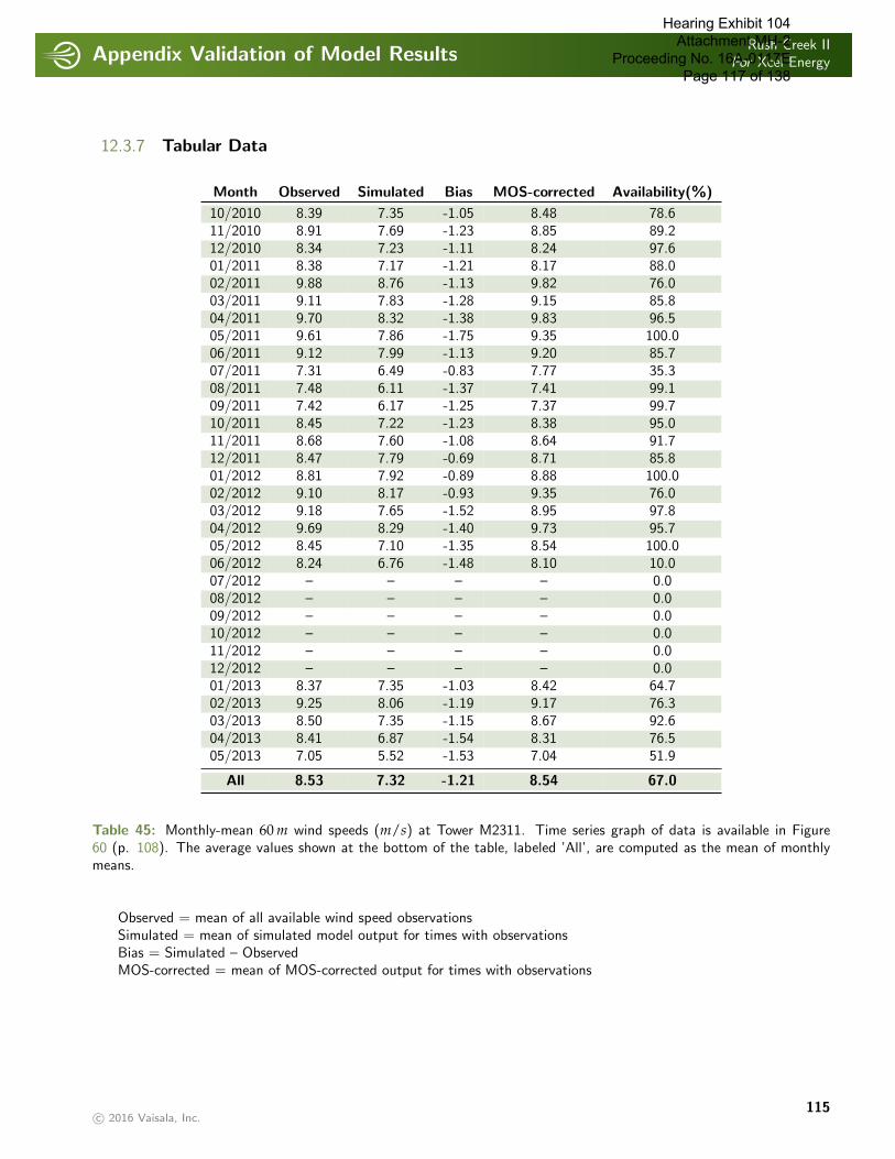
Appendix Validation of Model ResultsRush Creek II
For Xcel Energy
. . . . . . . . . . . . . . . . . . . . . . . . . . . . . . . . . . . . . . . . . . . . . . . . . . . . . . . . . . . . . . . . . . . . . . . . . . . . . . . . . . . . . . . . . . . . . . . . . . . . . . . . . . . . . . . . . .
12.3.7 Tabular Data
Month Observed Simulated Bias MOS-corrected Availability(%)
10/2010 8.39 7.35 -1.05 8.48 78.611/2010 8.91 7.69 -1.23 8.85 89.212/2010 8.34 7.23 -1.11 8.24 97.601/2011 8.38 7.17 -1.21 8.17 88.002/2011 9.88 8.76 -1.13 9.82 76.003/2011 9.11 7.83 -1.28 9.15 85.804/2011 9.70 8.32 -1.38 9.83 96.505/2011 9.61 7.86 -1.75 9.35 100.006/2011 9.12 7.99 -1.13 9.20 85.707/2011 7.31 6.49 -0.83 7.77 35.308/2011 7.48 6.11 -1.37 7.41 99.109/2011 7.42 6.17 -1.25 7.37 99.710/2011 8.45 7.22 -1.23 8.38 95.011/2011 8.68 7.60 -1.08 8.64 91.712/2011 8.47 7.79 -0.69 8.71 85.801/2012 8.81 7.92 -0.89 8.88 100.002/2012 9.10 8.17 -0.93 9.35 76.003/2012 9.18 7.65 -1.52 8.95 97.804/2012 9.69 8.29 -1.40 9.73 95.705/2012 8.45 7.10 -1.35 8.54 100.006/2012 8.24 6.76 -1.48 8.10 10.007/2012 – – – – 0.008/2012 – – – – 0.009/2012 – – – – 0.010/2012 – – – – 0.011/2012 – – – – 0.012/2012 – – – – 0.001/2013 8.37 7.35 -1.03 8.42 64.702/2013 9.25 8.06 -1.19 9.17 76.303/2013 8.50 7.35 -1.15 8.67 92.604/2013 8.41 6.87 -1.54 8.31 76.505/2013 7.05 5.52 -1.53 7.04 51.9
All 8.53 7.32 -1.21 8.54 67.0
Table 45: Monthly-mean 60 m wind speeds (m/s) at Tower M2311. Time series graph of data is available in Figure60 (p. 108). The average values shown at the bottom of the table, labeled ’All’, are computed as the mean of monthlymeans.
Observed = mean of all available wind speed observationsSimulated = mean of simulated model output for times with observationsBias = Simulated – ObservedMOS-corrected = mean of MOS-corrected output for times with observations
c© 2016 Vaisala, Inc.115
Hearing Exhibit 104 Attachment MH-2
Proceeding No. 16A-0117E Page 117 of 138

Appendix Validation of Model ResultsRush Creek II
For Xcel Energy
. . . . . . . . . . . . . . . . . . . . . . . . . . . . . . . . . . . . . . . . . . . . . . . . . . . . . . . . . . . . . . . . . . . . . . . . . . . . . . . . . . . . . . . . . . . . . . . . . . . . . . . . . . . . . . . . . .
Observations
Hou
r of
Day
(M
ST
)
012
34
567
89
101112
1314
151617
1819202122
23
Avg
Jan
Jan
Feb
Feb
Mar
Mar
Apr
Apr
May
May
Jun
Jun
Jly
Jly
Aug
Aug
Sep
Sep
Oct
Oct
Nov
Nov
Dec
Dec
Avg
Avg
8.32
8.69
8.70
8.37
8.47
8.73
8.92
9.03
9.17
9.01
8.86
8.99
8.86
8.87
9.05
8.42
8.06
8.24
8.49
8.37
7.96
8.01
7.69
7.82
8.55
9.00
9.18
9.77
9.90
9.61
9.75
9.96
9.68
9.89
9.78
9.65
9.18
9.25
9.05
8.91
8.37
8.72
9.09
9.89
9.53
9.52
9.50
9.46
9.17
9.41
8.88
9.71
9.97
9.79
9.99
9.90
9.75
9.31
9.35
9.46
9.43
9.22
9.25
8.98
8.17
8.21
8.10
8.24
7.84
7.87
8.06
8.20
8.24
8.21
8.93
8.87
9.12
9.71
9.75
10.32
10.07
10.14
10.24
10.09
10.16
9.85
9.43
9.54
9.14
9.00
8.57
8.47
8.46
8.48
8.78
8.56
8.77
9.32
9.17
9.33
9.32
9.68
10.27
10.23
9.64
9.71
9.27
9.36
9.14
8.71
8.45
8.20
7.96
7.44
7.30
7.54
7.78
7.84
7.85
8.03
8.05
8.21
8.37
8.55
8.62
10.13
10.27
9.76
10.24
10.40
10.38
10.46
10.07
9.69
9.05
9.13
9.26
9.04
7.95
7.85
7.99
7.82
7.40
7.74
7.50
8.18
8.07
9.36
8.91
9.03
−−
−−
−−
−−
−−
−−
−−
−−
−−
−−
−−
−−
−−
−−
−−
−−
−−
−−
−−
−−
−−
−−
−−
−−
−−
8.07
8.87
9.48
9.29
9.35
8.75
8.48
7.46
6.85
6.96
7.15
7.52
7.50
6.70
6.73
7.00
6.83
6.66
6.44
6.29
6.43
6.45
6.88
7.42
7.48
7.33
7.93
7.90
7.95
8.12
8.02
7.56
7.50
7.47
7.46
7.74
8.24
8.09
7.97
7.29
7.54
7.11
7.07
6.67
6.66
6.57
6.58
6.46
6.98
7.42
8.61
8.88
9.24
8.95
8.57
8.62
8.54
8.60
8.65
8.59
8.59
8.92
8.60
8.27
7.42
7.59
7.75
7.96
8.31
8.36
8.07
8.34
8.33
8.37
8.42
9.83
9.22
9.29
9.22
9.60
9.63
9.64
9.63
9.45
9.19
8.98
9.06
8.79
8.68
7.95
7.29
7.64
7.54
8.17
8.26
8.41
8.73
8.56
8.60
8.79
8.37
8.54
8.35
8.56
8.29
8.41
8.81
8.92
9.07
9.31
9.38
9.15
9.25
9.04
9.12
8.41
7.45
7.47
7.72
7.68
7.33
7.38
7.66
8.07
8.40
8.81
9.14
9.40
9.37
9.37
9.35
9.32
9.21
9.15
9.06
8.95
8.87
8.80
8.47
8.19
7.97
7.88
7.95
8.11
8.11
8.06
8.18
8.33
8.39
8.53
5 6 7 8 9 10 11 12Wind Speed
m/s
Figure 67: Hourly-mean values of observed 60 m wind speed at Tower M2311. Hours missing greater than 50% of theavailable observations are not plotted. The vertical axis is Mountain Standard Time (MST). Time seriesgraphs of data are available in Figures 65 and 66 (p. 113 and 114).
c© 2016 Vaisala, Inc.116
Hearing Exhibit 104 Attachment MH-2
Proceeding No. 16A-0117E Page 118 of 138
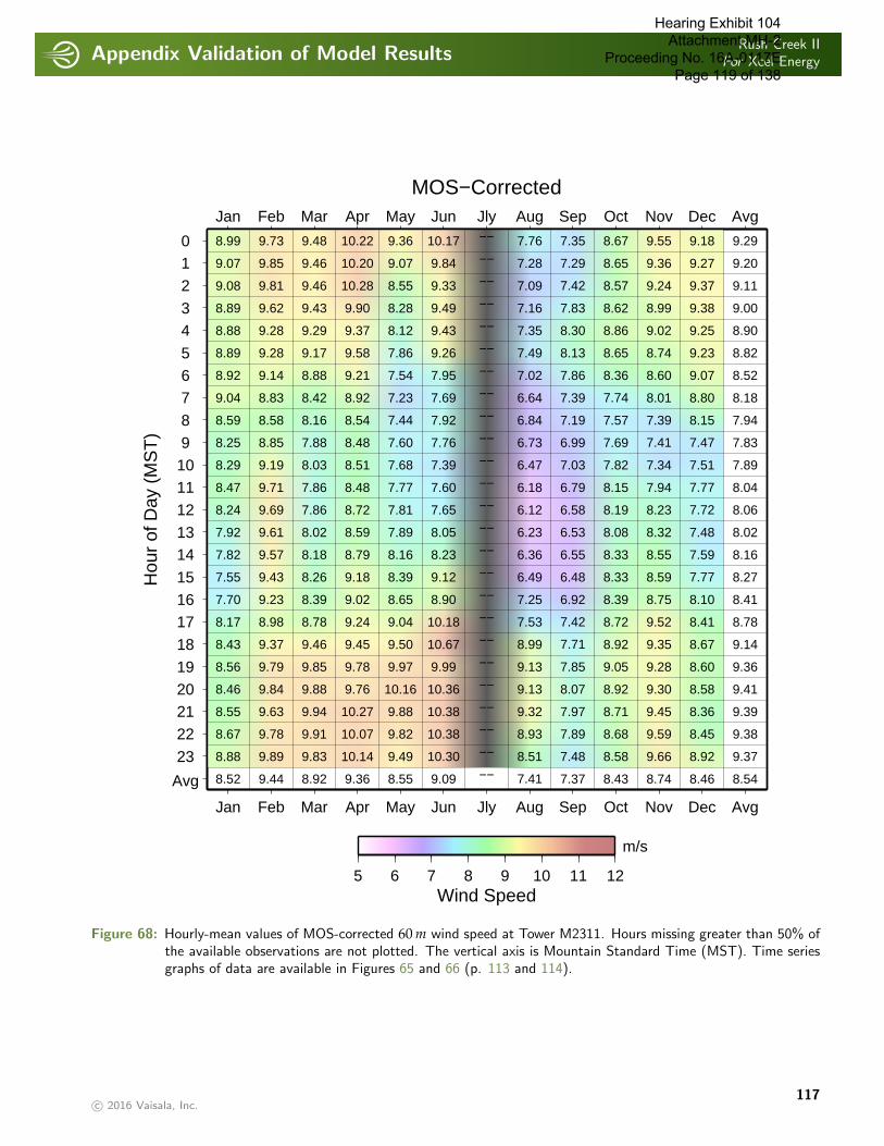
Appendix Validation of Model ResultsRush Creek II
For Xcel Energy
. . . . . . . . . . . . . . . . . . . . . . . . . . . . . . . . . . . . . . . . . . . . . . . . . . . . . . . . . . . . . . . . . . . . . . . . . . . . . . . . . . . . . . . . . . . . . . . . . . . . . . . . . . . . . . . . . .
MOS−Corrected
Hou
r of
Day
(M
ST
)
012
34
567
89
101112
1314
151617
1819202122
23
Avg
Jan
Jan
Feb
Feb
Mar
Mar
Apr
Apr
May
May
Jun
Jun
Jly
Jly
Aug
Aug
Sep
Sep
Oct
Oct
Nov
Nov
Dec
Dec
Avg
Avg
8.17
8.43
8.56
8.46
8.55
8.67
8.88
8.99
9.07
9.08
8.89
8.88
8.89
8.92
9.04
8.59
8.25
8.29
8.47
8.24
7.92
7.82
7.55
7.70
8.52
8.98
9.37
9.79
9.84
9.63
9.78
9.89
9.73
9.85
9.81
9.62
9.28
9.28
9.14
8.83
8.58
8.85
9.19
9.71
9.69
9.61
9.57
9.43
9.23
9.44
8.78
9.46
9.85
9.88
9.94
9.91
9.83
9.48
9.46
9.46
9.43
9.29
9.17
8.88
8.42
8.16
7.88
8.03
7.86
7.86
8.02
8.18
8.26
8.39
8.92
9.24
9.45
9.78
9.76
10.27
10.07
10.14
10.22
10.20
10.28
9.90
9.37
9.58
9.21
8.92
8.54
8.48
8.51
8.48
8.72
8.59
8.79
9.18
9.02
9.36
9.04
9.50
9.97
10.16
9.88
9.82
9.49
9.36
9.07
8.55
8.28
8.12
7.86
7.54
7.23
7.44
7.60
7.68
7.77
7.81
7.89
8.16
8.39
8.65
8.55
10.18
10.67
9.99
10.36
10.38
10.38
10.30
10.17
9.84
9.33
9.49
9.43
9.26
7.95
7.69
7.92
7.76
7.39
7.60
7.65
8.05
8.23
9.12
8.90
9.09
−−
−−
−−
−−
−−
−−
−−
−−
−−
−−
−−
−−
−−
−−
−−
−−
−−
−−
−−
−−
−−
−−
−−
−−
−−
7.53
8.99
9.13
9.13
9.32
8.93
8.51
7.76
7.28
7.09
7.16
7.35
7.49
7.02
6.64
6.84
6.73
6.47
6.18
6.12
6.23
6.36
6.49
7.25
7.41
7.42
7.71
7.85
8.07
7.97
7.89
7.48
7.35
7.29
7.42
7.83
8.30
8.13
7.86
7.39
7.19
6.99
7.03
6.79
6.58
6.53
6.55
6.48
6.92
7.37
8.72
8.92
9.05
8.92
8.71
8.68
8.58
8.67
8.65
8.57
8.62
8.86
8.65
8.36
7.74
7.57
7.69
7.82
8.15
8.19
8.08
8.33
8.33
8.39
8.43
9.52
9.35
9.28
9.30
9.45
9.59
9.66
9.55
9.36
9.24
8.99
9.02
8.74
8.60
8.01
7.39
7.41
7.34
7.94
8.23
8.32
8.55
8.59
8.75
8.74
8.41
8.67
8.60
8.58
8.36
8.45
8.92
9.18
9.27
9.37
9.38
9.25
9.23
9.07
8.80
8.15
7.47
7.51
7.77
7.72
7.48
7.59
7.77
8.10
8.46
8.78
9.14
9.36
9.41
9.39
9.38
9.37
9.29
9.20
9.11
9.00
8.90
8.82
8.52
8.18
7.94
7.83
7.89
8.04
8.06
8.02
8.16
8.27
8.41
8.54
5 6 7 8 9 10 11 12Wind Speed
m/s
Figure 68: Hourly-mean values of MOS-corrected 60 m wind speed at Tower M2311. Hours missing greater than 50% ofthe available observations are not plotted. The vertical axis is Mountain Standard Time (MST). Time seriesgraphs of data are available in Figures 65 and 66 (p. 113 and 114).
c© 2016 Vaisala, Inc.117
Hearing Exhibit 104 Attachment MH-2
Proceeding No. 16A-0117E Page 119 of 138

Appendix Validation of Model ResultsRush Creek II
For Xcel Energy
. . . . . . . . . . . . . . . . . . . . . . . . . . . . . . . . . . . . . . . . . . . . . . . . . . . . . . . . . . . . . . . . . . . . . . . . . . . . . . . . . . . . . . . . . . . . . . . . . . . . . . . . . . . . . . . . . .
Win
dSpee
dN
NN
EN
EEN
EE
ESE
SE
SSE
SSSW
SW
WSW
WW
NW
NW
NN
WA
ll(m
/s)
0-
0.5
0.00
0.01
0.01
0.00
0.01
0.00
0.00
0.00
0.00
0.01
0.00
0.00
0.00
0.00
0.01
0.00
0.04
0.5
-1.
50.
060.
080.
060.
080.
040.
030.
020.
030.
020.
040.
040.
040.
070.
040.
030.
060.
741.
5-
2.5
0.12
0.23
0.35
0.13
0.17
0.13
0.09
0.13
0.14
0.15
0.19
0.12
0.18
0.16
0.13
0.17
2.61
2.5
-3.
50.
360.
340.
400.
240.
260.
190.
200.
230.
310.
370.
280.
230.
190.
320.
220.
334.
453.
5-
4.5
0.52
0.33
0.43
0.35
0.32
0.31
0.24
0.40
0.50
0.54
0.45
0.38
0.37
0.30
0.40
0.43
6.26
4.5
-5.
50.
560.
520.
630.
390.
400.
220.
340.
550.
700.
660.
500.
380.
480.
440.
420.
597.
785.
5-
6.5
0.73
0.38
0.57
0.34
0.35
0.28
0.52
0.68
0.93
0.77
0.57
0.47
0.42
0.43
0.53
0.73
8.72
6.5
-7.
50.
720.
490.
520.
340.
320.
390.
380.
871.
111.
050.
630.
520.
430.
490.
500.
819.
577.
5-
8.5
0.89
0.62
0.56
0.26
0.24
0.39
0.64
0.79
1.24
1.01
0.80
0.48
0.41
0.42
0.47
0.96
10.1
78.
5-
9.5
0.81
0.63
0.61
0.27
0.23
0.39
0.42
0.94
1.32
1.09
0.63
0.39
0.30
0.47
0.41
0.88
9.78
9.5
-10
.50.
750.
560.
330.
240.
290.
380.
520.
981.
050.
810.
490.
420.
290.
370.
471.
129.
0810
.5-
11.5
0.83
0.45
0.30
0.17
0.18
0.32
0.59
0.82
0.85
0.65
0.45
0.26
0.26
0.35
0.40
1.09
7.96
11.5
-12
.50.
870.
360.
170.
130.
120.
270.
610.
810.
560.
340.
230.
140.
160.
270.
391.
066.
4912
.5-
13.5
0.74
0.28
0.07
0.03
0.08
0.26
0.54
0.71
0.33
0.19
0.20
0.10
0.05
0.13
0.34
0.94
4.98
13.5
-14
.50.
630.
200.
060.
010.
040.
150.
450.
490.
170.
090.
130.
050.
020.
120.
190.
753.
5214
.5-
15.5
0.52
0.08
0.03
0.01
0.02
0.07
0.26
0.34
0.08
0.07
0.11
0.04
0.02
0.05
0.11
0.54
2.36
15.5
-16
.50.
260.
100.
010.
000.
010.
060.
150.
240.
050.
020.
040.
020.
010.
040.
110.
361.
4916
.5-
17.5
0.18
0.04
0.01
0.00
0.02
0.03
0.17
0.12
0.07
0.02
0.03
0.01
0.00
0.03
0.06
0.28
1.06
17.5
-18
.50.
150.
030.
010.
000.
000.
010.
070.
080.
010.
010.
020.
020.
010.
000.
060.
240.
7118
.5-
19.5
0.08
0.00
0.01
0.00
0.00
0.01
0.04
0.02
0.03
0.02
0.01
0.00
0.00
0.00
0.03
0.18
0.43
19.5
-20
.50.
030.
010.
010.
000.
000.
000.
020.
030.
020.
010.
010.
000.
000.
010.
050.
120.
3120
.5-
21.5
0.05
0.00
0.00
0.00
0.00
0.00
0.01
0.03
0.02
0.00
0.00
0.01
0.00
0.00
0.03
0.12
0.27
21.5
-22
.50.
030.
000.
000.
000.
000.
000.
010.
010.
020.
010.
010.
000.
000.
000.
030.
080.
1922
.5-
23.5
0.03
0.00
0.00
0.00
0.00
0.00
0.01
0.01
0.02
0.01
0.00
0.01
0.00
0.00
0.01
0.09
0.18
23.5
-24
.50.
010.
000.
000.
000.
000.
000.
010.
010.
010.
010.
000.
000.
000.
000.
010.
040.
09>
24.5
0.01
0.00
0.00
0.00
0.00
0.00
0.00
0.00
0.01
0.00
0.00
0.00
0.00
0.01
0.01
0.04
0.08
Table
46:
Distr
ibution
ofob
serv
ed60
mw
ind
spee
dby
direc
tion
atTow
erM
2311
.H
isto
gram
ofdat
ais
avai
lable
inFig
ure
61(p
.10
9).
c© 2016 Vaisala, Inc.118
Hearing Exhibit 104 Attachment MH-2
Proceeding No. 16A-0117E Page 120 of 138

Appendix Validation of Model ResultsRush Creek II
For Xcel Energy
. . . . . . . . . . . . . . . . . . . . . . . . . . . . . . . . . . . . . . . . . . . . . . . . . . . . . . . . . . . . . . . . . . . . . . . . . . . . . . . . . . . . . . . . . . . . . . . . . . . . . . . . . . . . . . . . . .
Win
dSpee
dN
NN
EN
EEN
EE
ESE
SE
SSE
SSSW
SW
WSW
WW
NW
NW
NN
WA
ll(m
/s)
0-
0.5
0.00
0.00
0.00
0.00
0.00
0.00
0.01
0.00
0.00
0.01
0.00
0.00
0.01
0.00
0.01
0.00
0.04
0.5
-1.
50.
030.
020.
030.
040.
080.
080.
130.
040.
050.
050.
020.
040.
030.
030.
030.
030.
741.
5-
2.5
0.10
0.15
0.11
0.16
0.18
0.28
0.19
0.21
0.23
0.19
0.17
0.17
0.11
0.10
0.12
0.09
2.56
2.5
-3.
50.
260.
290.
190.
240.
260.
250.
150.
260.
330.
390.
400.
400.
330.
260.
220.
244.
473.
5-
4.5
0.39
0.28
0.31
0.35
0.26
0.29
0.25
0.35
0.47
0.64
0.62
0.52
0.43
0.49
0.33
0.40
6.38
4.5
-5.
50.
430.
500.
400.
230.
330.
310.
430.
550.
640.
770.
720.
630.
590.
430.
430.
507.
905.
5-
6.5
0.61
0.54
0.38
0.41
0.28
0.29
0.39
0.66
0.88
0.73
0.66
0.68
0.61
0.49
0.54
0.59
8.73
6.5
-7.
50.
670.
620.
300.
350.
380.
290.
520.
770.
880.
960.
750.
630.
500.
630.
660.
659.
567.
5-
8.5
0.90
0.46
0.40
0.41
0.32
0.29
0.52
1.09
1.21
1.00
0.54
0.34
0.53
0.64
0.63
0.88
10.1
68.
5-
9.5
0.97
0.66
0.31
0.22
0.24
0.21
0.57
1.07
1.09
0.84
0.40
0.22
0.39
0.80
0.76
0.94
9.71
9.5
-10
.50.
890.
470.
460.
280.
200.
320.
501.
021.
020.
510.
280.
200.
380.
790.
601.
079.
0010
.5-
11.5
0.84
0.55
0.45
0.15
0.19
0.29
0.54
1.08
0.75
0.31
0.19
0.12
0.13
0.71
0.73
0.89
7.93
11.5
-12
.50.
970.
550.
220.
120.
100.
230.
620.
730.
450.
220.
150.
150.
130.
420.
610.
796.
4712
.5-
13.5
0.72
0.54
0.14
0.07
0.06
0.19
0.54
0.66
0.31
0.20
0.11
0.05
0.10
0.29
0.38
0.63
4.98
13.5
-14
.50.
570.
360.
100.
020.
090.
070.
430.
450.
270.
090.
100.
060.
030.
080.
240.
563.
5114
.5-
15.5
0.43
0.22
0.06
0.01
0.02
0.04
0.21
0.30
0.17
0.08
0.04
0.04
0.03
0.06
0.12
0.52
2.36
15.5
-16
.50.
330.
130.
020.
010.
010.
010.
090.
190.
100.
060.
040.
010.
010.
030.
080.
361.
4916
.5-
17.5
0.24
0.08
0.02
0.02
0.01
0.02
0.11
0.09
0.05
0.04
0.03
0.01
0.02
0.02
0.10
0.22
1.06
17.5
-18
.50.
100.
030.
010.
000.
000.
030.
080.
100.
020.
020.
030.
010.
000.
010.
030.
260.
7118
.5-
19.5
0.07
0.01
0.00
0.00
0.00
0.00
0.05
0.03
0.03
0.01
0.03
0.01
0.00
0.01
0.02
0.15
0.43
19.5
-20
.50.
060.
000.
010.
000.
000.
000.
020.
030.
020.
030.
010.
000.
010.
000.
030.
110.
3120
.5-
21.5
0.04
0.00
0.00
0.00
0.00
0.01
0.00
0.03
0.02
0.00
0.03
0.00
0.00
0.01
0.01
0.13
0.27
21.5
-22
.50.
040.
000.
000.
000.
000.
000.
010.
010.
010.
010.
010.
000.
000.
000.
020.
080.
1922
.5-
23.5
0.05
0.00
0.00
0.00
0.00
0.01
0.00
0.01
0.01
0.01
0.01
0.00
0.00
0.00
0.02
0.06
0.18
23.5
-24
.50.
010.
000.
000.
000.
000.
000.
010.
000.
020.
030.
000.
000.
000.
000.
010.
020.
09>
24.5
0.00
0.00
0.00
0.00
0.00
0.00
0.00
0.00
0.05
0.00
0.00
0.00
0.00
0.01
0.01
0.01
0.08
Table
47:
Distr
ibution
ofM
OS-c
orre
cted
60m
win
dsp
eed
bydirec
tion
atTow
erM
2311
.A
llm
odel
valu
esar
eco
mpute
don
lyfo
rtim
esw
ith
valid
obse
rvat
ions.
Histo
gram
ofdat
ais
avai
lable
inFig
ure
61(p
.10
9).
c© 2016 Vaisala, Inc.119
Hearing Exhibit 104 Attachment MH-2
Proceeding No. 16A-0117E Page 121 of 138

Appendix Validation of Model ResultsRush Creek II
For Xcel Energy
. . . . . . . . . . . . . . . . . . . . . . . . . . . . . . . . . . . . . . . . . . . . . . . . . . . . . . . . . . . . . . . . . . . . . . . . . . . . . . . . . . . . . . . . . . . . . . . . . . . . . . . . . . . . . . . . . .
Sector Mean Speed(m/s) Weibull Scale(A) Weibull Shape(k) Frequency(%)
N 9.90 11.15 2.51 10.02NNE 8.23 9.29 2.39 5.77NE 6.89 7.78 2.32 5.18ENE 6.65 7.50 2.39 3.02E 6.93 7.82 2.24 3.12
ESE 8.51 9.59 2.51 3.90SE 9.98 11.22 2.74 6.34SSE 9.58 10.77 2.79 9.36S 8.49 9.55 2.71 9.62
SSW 7.91 8.89 2.69 7.99SW 7.95 8.96 2.49 5.86
WSW 7.51 8.46 2.49 4.11W 6.99 7.88 2.48 3.68
WNW 7.82 8.82 2.30 4.47NW 9.00 10.17 2.22 5.43
NNW 10.62 11.97 2.49 12.12
ALL 8.53 9.63 2.33 100.00
Table 48: Observed 60 m mean wind speed, Weibull parameters, and frequency at Tower M2311. Blank values correspondto times with less than 10 data points. Wind rose of data is available in Figure 62 (p. 110).
Sector Mean Speed(m/s) Weibull Scale(A) Weibull Shape(k) Frequency(%)
N 10.22 11.49 2.71 9.80NNE 9.11 10.25 2.66 6.52NE 8.12 9.14 2.56 3.95ENE 6.97 7.86 2.40 3.12E 6.95 7.84 2.24 3.03
ESE 7.61 8.59 2.02 3.53SE 9.49 10.70 2.48 6.42SSE 9.45 10.62 2.78 9.80S 8.60 9.71 2.37 9.12
SSW 7.58 8.56 2.32 7.25SW 7.17 8.10 2.15 5.37
WSW 6.54 7.38 2.26 4.34W 6.94 7.82 2.49 4.40
WNW 8.39 9.41 2.86 6.33NW 9.12 10.27 2.60 6.76
NNW 10.64 11.99 2.55 10.27
ALL 8.54 9.64 2.33 100.00
Table 49: MOS-corrected 60 m mean wind speed, Weibull parameters, and frequency at Tower M2311. All MOS-correctedmodel values are computed only for times with valid observations; blank values correspond to times with lessthan 10 data points. Wind rose of data is available in Figure 62 (p. 110).
c© 2016 Vaisala, Inc.120
Hearing Exhibit 104 Attachment MH-2
Proceeding No. 16A-0117E Page 122 of 138
Appendix Validation of Model ResultsRush Creek II
For Xcel Energy
. . . . . . . . . . . . . . . . . . . . . . . . . . . . . . . . . . . . . . . . . . . . . . . . . . . . . . . . . . . . . . . . . . . . . . . . . . . . . . . . . . . . . . . . . . . . . . . . . . . . . . . . . . . . . . . . . .
12.4 Validation of Model Results at Tower M2313
This section examines the quality of the NWP simulations used at a single point within the study area. For this section,the observations were taken at Tower M2313 (latitude 39.07764, longitude -103.23864).
The average observed wind speed (for all valid observational times) at 60.0 m during the 28 months of the period ofrecord (October, 2010 to January, 2013) is 8.54 m/s with an hourly standard deviation of 4.00 m/s at Tower M2313. Thiscompares to a modeled 60 m wind speed of 7.23 m/s with a 3.53 m/s standard deviation for these same times.
Based on a comparison of the NWP model output with observations from each of the meteorological towers for whichdata were provided, Model Output Statistics (MOS) was constructed. MOS uses a multilinear regression model designedto remove the bias and adjust the variance of the raw NWP simulated wind speed and direction. Applying this statisticalmodel to the simulated data at Tower M2313 results in a MOS-corrected mean value of 8.56 m/s and an hourly standarddeviation of 4.00 m/s.
This section presents a comparison of the simulated winds with the observations at the reference tower (Tower M2313).The focus of the verification is on the model’s ability to reproduce the observed variability of the wind resource at daily andmonthly time scales, while preserving the distribution of hourly wind speeds and the diurnal characteristics of the wind.
c© 2016 Vaisala, Inc.121
Hearing Exhibit 104 Attachment MH-2
Proceeding No. 16A-0117E Page 123 of 138

Appendix Validation of Model ResultsRush Creek II
For Xcel Energy
. . . . . . . . . . . . . . . . . . . . . . . . . . . . . . . . . . . . . . . . . . . . . . . . . . . . . . . . . . . . . . . . . . . . . . . . . . . . . . . . . . . . . . . . . . . . . . . . . . . . . . . . . . . . . . . . . .
12.4.1 Observational Data
Approximately 28 months of wind speed data at 60.0 meters and wind direction data at 58.0 meters (October, 2010 toJanuary, 2013) from a meteorological tower (Tower M2313) at Rush Creek II were used in this analysis. This tower will bereferred to as the reference tower throughout this section. The data at 60 m were used to assess the quality of the modelsimulations at 60 m.
It should be noted that meteorological observations provided to 3TIER are not allowed to influence the raw model simu-lations.
12.4.2 Model Validation Statistics
Table 50 presents some basic statistical measures of the model performance relative to the measured winds at the referencetower during the observational period. Also shown are values (labeled “MOS-corrected”) for model data with the statisticalmodel applied. For reference, the correlation of the reference tower data to itself is perfect and hence the explained variance(r2) value is 1.0.
The observed and modeled winds in this section represent the mean of all times during the month for which a valid windspeed or direction observation was available. Therefore they should not be interpreted as estimates of the true winds atthe site, but rather a verification of the model’s ability to reproduce the available observations. Any month or hour missinggreater than 50% of the available observations is omitted from the following figures, tables, and statistics.
Comparison Value
Correlation of monthly-mean simulated wind speed to observed 0.94RMS error of monthly-mean simulated wind speed 1.29 m/sCorrelation of monthly-mean MOS-corrected wind speed to observed 0.98RMS error of monthly-mean MOS-corrected wind speed 0.13 m/s
Correlation of daily-mean simulated wind speed to observed 0.89RMS error of daily-mean simulated wind speed 1.74 m/sCorrelation of daily-mean MOS-corrected wind speed to observed 0.89RMS error of daily-mean MOS-corrected wind speed 1.20 m/s
Table 50: Correlation and root mean square (RMS) error statistics of modeled wind speeds.
c© 2016 Vaisala, Inc.122
Hearing Exhibit 104 Attachment MH-2
Proceeding No. 16A-0117E Page 124 of 138
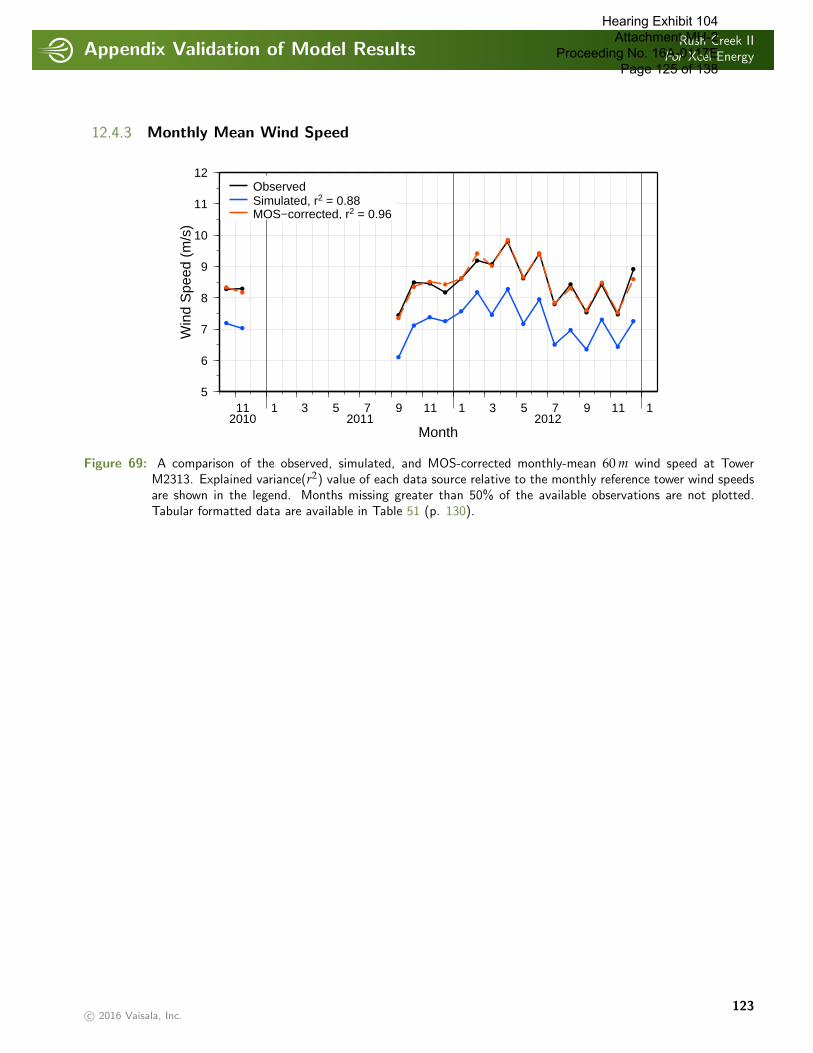
Appendix Validation of Model ResultsRush Creek II
For Xcel Energy
. . . . . . . . . . . . . . . . . . . . . . . . . . . . . . . . . . . . . . . . . . . . . . . . . . . . . . . . . . . . . . . . . . . . . . . . . . . . . . . . . . . . . . . . . . . . . . . . . . . . . . . . . . . . . . . . . .
12.4.3 Monthly Mean Wind Speed
11 1 3 5 7 9 11 1 3 5 7 9 11 1
Month2010 2011 2012
5
6
7
8
9
10
11
12W
ind
Spe
ed (
m/s
)ObservedSimulated, r2 = 0.88MOS−corrected, r2 = 0.96
Figure 69: A comparison of the observed, simulated, and MOS-corrected monthly-mean 60 m wind speed at TowerM2313. Explained variance(r2) value of each data source relative to the monthly reference tower wind speedsare shown in the legend. Months missing greater than 50% of the available observations are not plotted.Tabular formatted data are available in Table 51 (p. 130).
c© 2016 Vaisala, Inc.123
Hearing Exhibit 104 Attachment MH-2
Proceeding No. 16A-0117E Page 125 of 138
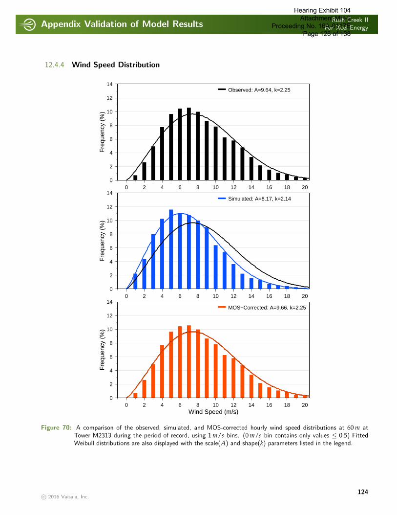
Appendix Validation of Model ResultsRush Creek II
For Xcel Energy
. . . . . . . . . . . . . . . . . . . . . . . . . . . . . . . . . . . . . . . . . . . . . . . . . . . . . . . . . . . . . . . . . . . . . . . . . . . . . . . . . . . . . . . . . . . . . . . . . . . . . . . . . . . . . . . . . .
12.4.4 Wind Speed Distribution
0 2 4 6 8 10 12 14 16 18 200
2
4
6
8
10
12
14
Fre
quen
cy (
%)
Observed: A=9.64, k=2.25
0 2 4 6 8 10 12 14 16 18 200
2
4
6
8
10
12
14
Fre
quen
cy (
%)
Simulated: A=8.17, k=2.14
0 2 4 6 8 10 12 14 16 18 20Wind Speed (m/s)
0
2
4
6
8
10
12
14
Fre
quen
cy (
%)
MOS−Corrected: A=9.66, k=2.25
Figure 70: A comparison of the observed, simulated, and MOS-corrected hourly wind speed distributions at 60 m atTower M2313 during the period of record, using 1 m/s bins. (0 m/s bin contains only values ≤ 0.5) FittedWeibull distributions are also displayed with the scale(A) and shape(k) parameters listed in the legend.
c© 2016 Vaisala, Inc.124
Hearing Exhibit 104 Attachment MH-2
Proceeding No. 16A-0117E Page 126 of 138

Appendix Validation of Model ResultsRush Creek II
For Xcel Energy
. . . . . . . . . . . . . . . . . . . . . . . . . . . . . . . . . . . . . . . . . . . . . . . . . . . . . . . . . . . . . . . . . . . . . . . . . . . . . . . . . . . . . . . . . . . . . . . . . . . . . . . . . . . . . . . . . .
12.4.5 Wind Direction Distribution
Observed
S 10 %
EW
N
S 10 %
EW
N
SW
NW
SE
NE
Simulated
S 10 %
EW
N
S 10 %
EW
N
SW
NW
SE
NE
MOS−Corrected
S 10 %
EW
N
S 10 %
EW
N
SW
NW
SE
NE
Figure 71: Wind roses at 58 m at Tower M2313 for observational data and simulated model data, averaged over theperiod of record (October, 2010–January, 2013). Directional bins are 22.5◦ wide, and the radial contourinterval is 10%. Tabular formatted data, including mean wind speed values and Weibull parameters for eachwind direction sector, are available in Tables 54 and 55 (p. 135).
c© 2016 Vaisala, Inc.125
Hearing Exhibit 104 Attachment MH-2
Proceeding No. 16A-0117E Page 127 of 138
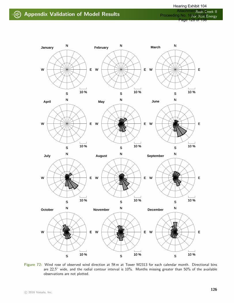
Appendix Validation of Model ResultsRush Creek II
For Xcel Energy
. . . . . . . . . . . . . . . . . . . . . . . . . . . . . . . . . . . . . . . . . . . . . . . . . . . . . . . . . . . . . . . . . . . . . . . . . . . . . . . . . . . . . . . . . . . . . . . . . . . . . . . . . . . . . . . . . .
S 10 %
EW
NOctober
S 10 %
EW
N
S 10 %
EW
NNovember
S 10 %
EW
N
S 10 %
EW
NDecember
S 10 %
EW
N
S 10 %
EW
NJuly
S 10 %
EW
N
S 10 %
EW
NAugust
S 10 %
EW
N
S 10 %
EW
NSeptember
S 10 %
EW
N
S 10 %
EW
NApril
S 10 %
EW
N
S 10 %
EW
NMay
S 10 %
EW
N
S 10 %
EW
NJune
S 10 %
EW
N
S 10 %
EW
NJanuary
S 10 %
EW
N
S 10 %
EW
NFebruary
S 10 %
EW
N
S 10 %
EW
NMarch
S 10 %
EW
N
Figure 72: Wind rose of observed wind direction at 58 m at Tower M2313 for each calendar month. Directional binsare 22.5◦ wide, and the radial contour interval is 10%. Months missing greater than 50% of the availableobservations are not plotted.
c© 2016 Vaisala, Inc.126
Hearing Exhibit 104 Attachment MH-2
Proceeding No. 16A-0117E Page 128 of 138
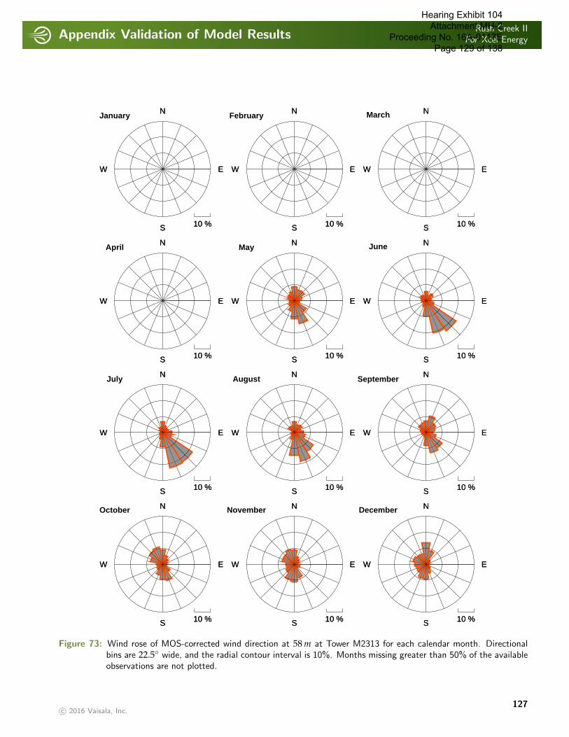
Appendix Validation of Model ResultsRush Creek II
For Xcel Energy
. . . . . . . . . . . . . . . . . . . . . . . . . . . . . . . . . . . . . . . . . . . . . . . . . . . . . . . . . . . . . . . . . . . . . . . . . . . . . . . . . . . . . . . . . . . . . . . . . . . . . . . . . . . . . . . . . .
S 10 %
EW
NOctober
S 10 %
EW
N
S 10 %
EW
NNovember
S 10 %
EW
N
S 10 %
EW
NDecember
S 10 %
EW
N
S 10 %
EW
NJuly
S 10 %
EW
N
S 10 %
EW
NAugust
S 10 %
EW
N
S 10 %
EW
NSeptember
S 10 %
EW
N
S 10 %
EW
NApril
S 10 %
EW
N
S 10 %
EW
NMay
S 10 %
EW
N
S 10 %
EW
NJune
S 10 %
EW
N
S 10 %
EW
NJanuary
S 10 %
EW
N
S 10 %
EW
NFebruary
S 10 %
EW
N
S 10 %
EW
NMarch
S 10 %
EW
N
Figure 73: Wind rose of MOS-corrected wind direction at 58 m at Tower M2313 for each calendar month. Directionalbins are 22.5◦ wide, and the radial contour interval is 10%. Months missing greater than 50% of the availableobservations are not plotted.
c© 2016 Vaisala, Inc.127
Hearing Exhibit 104 Attachment MH-2
Proceeding No. 16A-0117E Page 129 of 138

Appendix Validation of Model ResultsRush Creek II
For Xcel Energy
. . . . . . . . . . . . . . . . . . . . . . . . . . . . . . . . . . . . . . . . . . . . . . . . . . . . . . . . . . . . . . . . . . . . . . . . . . . . . . . . . . . . . . . . . . . . . . . . . . . . . . . . . . . . . . . . . .
12.4.6 Diurnal Variability of Wind Speed
0 4 8 12 16 20 24
Hour of Day (MST)
5
6
7
8
9
10
11
Win
d S
peed
(m
/s)
ObservedSimulatedMOS−corrected
Figure 74: A comparison of the diurnal cycle of observed, simulated, and MOS-corrected 60m wind speed at TowerM2313. Data are averaged over the period of record (October, 2010–January, 2013). Hours missing greaterthan 15% of the available observations are not plotted. The horizontal axis is Mountain Standard Time (MST).Tabular formatted data are available in Figures 76 and 77 (p. 131 and 132).
c© 2016 Vaisala, Inc.128
Hearing Exhibit 104 Attachment MH-2
Proceeding No. 16A-0117E Page 130 of 138
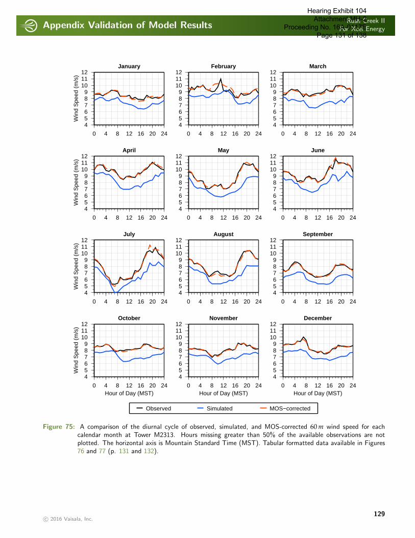
Appendix Validation of Model ResultsRush Creek II
For Xcel Energy
. . . . . . . . . . . . . . . . . . . . . . . . . . . . . . . . . . . . . . . . . . . . . . . . . . . . . . . . . . . . . . . . . . . . . . . . . . . . . . . . . . . . . . . . . . . . . . . . . . . . . . . . . . . . . . . . . .
January
0 4 8 12 16 20 24
456789
101112
Win
d S
peed
(m
/s)
February
0 4 8 12 16 20 24
456789
101112
March
0 4 8 12 16 20 24
456789
101112
April
0 4 8 12 16 20 24
456789
101112
Win
d S
peed
(m
/s)
May
0 4 8 12 16 20 24
456789
101112
June
0 4 8 12 16 20 24
456789
101112
July
0 4 8 12 16 20 24
456789
101112
Win
d S
peed
(m
/s)
August
0 4 8 12 16 20 24
456789
101112
September
0 4 8 12 16 20 24
456789
101112
October
0 4 8 12 16 20 24Hour of Day (MST)
456789
101112
Win
d S
peed
(m
/s)
November
0 4 8 12 16 20 24Hour of Day (MST)
456789
101112
Observed Simulated MOS−corrected
December
0 4 8 12 16 20 24Hour of Day (MST)
456789
101112
Figure 75: A comparison of the diurnal cycle of observed, simulated, and MOS-corrected 60 m wind speed for eachcalendar month at Tower M2313. Hours missing greater than 50% of the available observations are notplotted. The horizontal axis is Mountain Standard Time (MST). Tabular formatted data available in Figures76 and 77 (p. 131 and 132).
c© 2016 Vaisala, Inc.129
Hearing Exhibit 104 Attachment MH-2
Proceeding No. 16A-0117E Page 131 of 138
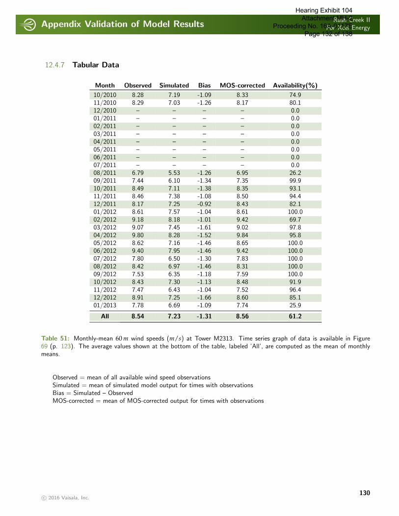
Appendix Validation of Model ResultsRush Creek II
For Xcel Energy
. . . . . . . . . . . . . . . . . . . . . . . . . . . . . . . . . . . . . . . . . . . . . . . . . . . . . . . . . . . . . . . . . . . . . . . . . . . . . . . . . . . . . . . . . . . . . . . . . . . . . . . . . . . . . . . . . .
12.4.7 Tabular Data
Month Observed Simulated Bias MOS-corrected Availability(%)
10/2010 8.28 7.19 -1.09 8.33 74.911/2010 8.29 7.03 -1.26 8.17 80.112/2010 – – – – 0.001/2011 – – – – 0.002/2011 – – – – 0.003/2011 – – – – 0.004/2011 – – – – 0.005/2011 – – – – 0.006/2011 – – – – 0.007/2011 – – – – 0.008/2011 6.79 5.53 -1.26 6.95 26.209/2011 7.44 6.10 -1.34 7.35 99.910/2011 8.49 7.11 -1.38 8.35 93.111/2011 8.46 7.38 -1.08 8.50 94.412/2011 8.17 7.25 -0.92 8.43 82.101/2012 8.61 7.57 -1.04 8.61 100.002/2012 9.18 8.18 -1.01 9.42 69.703/2012 9.07 7.45 -1.61 9.02 97.804/2012 9.80 8.28 -1.52 9.84 95.805/2012 8.62 7.16 -1.46 8.65 100.006/2012 9.40 7.95 -1.46 9.42 100.007/2012 7.80 6.50 -1.30 7.83 100.008/2012 8.42 6.97 -1.46 8.31 100.009/2012 7.53 6.35 -1.18 7.59 100.010/2012 8.43 7.30 -1.13 8.48 91.911/2012 7.47 6.43 -1.04 7.52 96.412/2012 8.91 7.25 -1.66 8.60 85.101/2013 7.78 6.69 -1.09 7.74 25.9
All 8.54 7.23 -1.31 8.56 61.2
Table 51: Monthly-mean 60 m wind speeds (m/s) at Tower M2313. Time series graph of data is available in Figure69 (p. 123). The average values shown at the bottom of the table, labeled ’All’, are computed as the mean of monthlymeans.
Observed = mean of all available wind speed observationsSimulated = mean of simulated model output for times with observationsBias = Simulated – ObservedMOS-corrected = mean of MOS-corrected output for times with observations
c© 2016 Vaisala, Inc.130
Hearing Exhibit 104 Attachment MH-2
Proceeding No. 16A-0117E Page 132 of 138
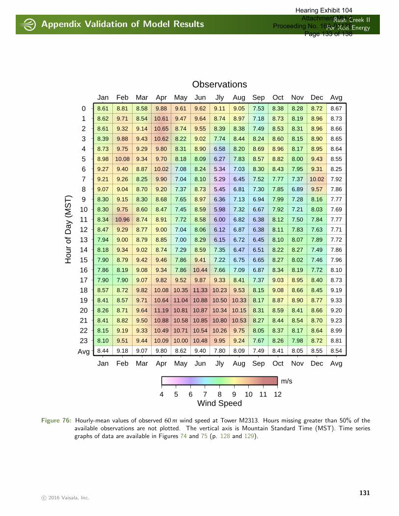
Appendix Validation of Model ResultsRush Creek II
For Xcel Energy
. . . . . . . . . . . . . . . . . . . . . . . . . . . . . . . . . . . . . . . . . . . . . . . . . . . . . . . . . . . . . . . . . . . . . . . . . . . . . . . . . . . . . . . . . . . . . . . . . . . . . . . . . . . . . . . . . .
Observations
Hou
r of
Day
(M
ST
)
012
34
567
89101112
1314
151617
1819202122
23
Avg
Jan
Jan
Feb
Feb
Mar
Mar
Apr
Apr
May
May
Jun
Jun
Jly
Jly
Aug
Aug
Sep
Sep
Oct
Oct
Nov
Nov
Dec
Dec
Avg
Avg
7.90
8.57
8.41
8.26
8.41
8.15
8.10
8.61
8.62
8.61
8.39
8.73
8.98
9.27
9.21
9.07
8.30
8.30
8.34
8.47
7.94
8.18
7.90
7.86
8.44
7.90
8.72
8.57
8.71
8.82
9.19
9.51
8.81
9.71
9.32
9.88
9.75
10.08
9.40
9.26
9.04
9.15
9.75
10.96
9.29
9.00
9.34
8.79
8.19
9.18
9.07
9.82
9.71
9.64
9.50
9.33
9.44
8.58
8.54
9.14
9.43
9.29
9.34
8.87
8.25
8.70
8.30
8.60
8.74
8.77
8.79
9.02
9.42
9.08
9.07
9.82
10.08
10.64
11.19
10.88
10.49
10.09
9.88
10.61
10.65
10.62
9.80
9.70
10.02
9.90
9.20
8.68
8.47
8.91
9.00
8.85
8.74
9.46
9.34
9.80
9.52
10.35
11.04
10.81
10.58
10.71
10.00
9.61
9.47
8.74
8.22
8.31
8.18
7.08
7.04
7.37
7.65
7.45
7.72
7.04
7.00
7.29
7.86
7.86
8.62
9.87
11.33
10.88
10.87
10.85
10.54
10.48
9.62
9.64
9.55
9.02
8.90
8.09
8.24
8.10
8.73
8.97
8.59
8.58
8.06
8.29
8.59
9.41
10.44
9.40
9.33
10.23
10.50
10.34
10.80
10.26
9.95
9.11
8.74
8.39
7.74
6.58
6.27
5.34
5.29
5.45
6.36
5.98
6.00
6.12
6.15
7.35
7.22
7.66
7.80
8.41
9.53
10.33
10.15
10.53
9.75
9.24
9.05
8.97
8.38
8.44
8.20
7.83
7.03
6.45
6.81
7.13
7.32
6.82
6.87
6.72
6.47
6.75
7.09
8.09
7.37
8.15
8.17
8.31
8.27
8.05
7.67
7.53
7.18
7.49
8.24
8.69
8.57
8.30
7.52
7.30
6.94
6.67
6.38
6.38
6.45
6.51
6.65
6.87
7.49
9.03
9.08
8.87
8.59
8.44
8.37
8.26
8.38
8.73
8.53
8.60
8.96
8.82
8.43
7.77
7.85
7.99
7.92
8.12
8.11
8.10
8.22
8.27
8.34
8.41
8.95
8.66
8.90
8.41
8.54
8.17
7.98
8.28
8.19
8.31
8.15
8.17
8.00
7.95
7.37
6.89
7.28
7.21
7.50
7.83
8.07
8.27
8.02
8.19
8.05
8.40
8.45
8.77
8.66
8.70
8.64
8.72
8.72
8.96
8.96
8.90
8.95
9.43
9.31
10.02
9.57
8.16
8.03
7.84
7.63
7.89
7.49
7.46
7.72
8.55
8.73
9.19
9.33
9.20
9.23
8.99
8.81
8.67
8.73
8.66
8.65
8.64
8.55
8.25
7.92
7.86
7.77
7.69
7.77
7.71
7.72
7.86
7.96
8.10
8.54
4 5 6 7 8 9 10 11 12Wind Speed
m/s
Figure 76: Hourly-mean values of observed 60 m wind speed at Tower M2313. Hours missing greater than 50% of theavailable observations are not plotted. The vertical axis is Mountain Standard Time (MST). Time seriesgraphs of data are available in Figures 74 and 75 (p. 128 and 129).
c© 2016 Vaisala, Inc.131
Hearing Exhibit 104 Attachment MH-2
Proceeding No. 16A-0117E Page 133 of 138
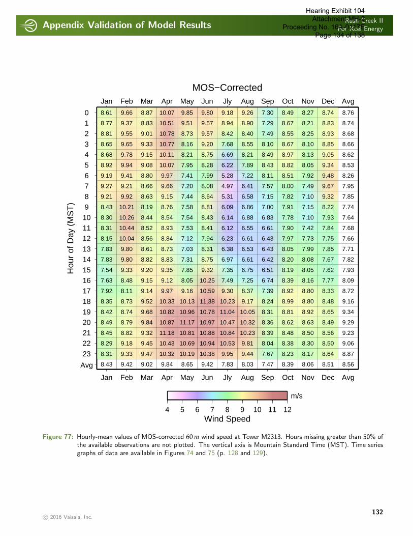
Appendix Validation of Model ResultsRush Creek II
For Xcel Energy
. . . . . . . . . . . . . . . . . . . . . . . . . . . . . . . . . . . . . . . . . . . . . . . . . . . . . . . . . . . . . . . . . . . . . . . . . . . . . . . . . . . . . . . . . . . . . . . . . . . . . . . . . . . . . . . . . .
MOS−Corrected
Hou
r of
Day
(M
ST
)
012
34
567
89
101112
1314
151617
1819202122
23
Avg
Jan
Jan
Feb
Feb
Mar
Mar
Apr
Apr
May
May
Jun
Jun
Jly
Jly
Aug
Aug
Sep
Sep
Oct
Oct
Nov
Nov
Dec
Dec
Avg
Avg
7.92
8.35
8.42
8.49
8.45
8.29
8.31
8.61
8.77
8.81
8.65
8.68
8.92
9.19
9.27
9.21
8.43
8.30
8.31
8.15
7.83
7.83
7.54
7.63
8.43
8.11
8.73
8.74
8.79
8.82
9.18
9.33
9.66
9.37
9.55
9.65
9.78
9.94
9.41
9.21
9.92
10.21
10.26
10.44
10.04
9.80
9.80
9.33
8.48
9.42
9.14
9.52
9.68
9.84
9.32
9.45
9.47
8.87
8.83
9.01
9.33
9.15
9.08
8.80
8.66
8.63
8.19
8.44
8.52
8.56
8.61
8.82
9.20
9.15
9.02
9.97
10.33
10.82
10.87
11.18
10.43
10.32
10.07
10.51
10.78
10.77
10.11
10.07
9.97
9.66
9.15
8.76
8.54
8.93
8.84
8.73
8.83
9.35
9.12
9.84
9.16
10.13
10.96
11.17
10.81
10.69
10.19
9.85
9.51
8.73
8.16
8.21
7.95
7.41
7.20
7.44
7.58
7.54
7.53
7.12
7.03
7.31
7.85
8.05
8.65
10.59
11.38
10.78
10.97
10.88
10.94
10.38
9.80
9.57
9.57
9.20
8.75
8.28
7.99
8.08
8.64
8.81
8.43
8.41
7.94
8.31
8.75
9.32
10.25
9.42
9.30
10.23
11.04
10.47
10.84
10.53
9.95
9.18
8.94
8.42
7.68
6.69
6.22
5.28
4.97
5.31
6.09
6.14
6.12
6.23
6.38
6.97
7.35
7.49
7.83
8.37
9.17
10.05
10.32
10.23
9.81
9.44
9.26
8.90
8.40
8.55
8.21
7.89
7.22
6.41
6.58
6.86
6.88
6.55
6.61
6.53
6.61
6.75
7.25
8.03
7.39
8.24
8.31
8.36
8.39
8.04
7.67
7.30
7.29
7.49
8.10
8.49
8.43
8.11
7.57
7.15
7.00
6.83
6.61
6.43
6.43
6.42
6.51
6.74
7.47
8.92
8.99
8.81
8.62
8.48
8.38
8.23
8.49
8.67
8.55
8.67
8.97
8.82
8.51
8.00
7.82
7.91
7.78
7.90
7.97
8.05
8.20
8.19
8.39
8.39
8.80
8.80
8.92
8.63
8.50
8.30
8.17
8.27
8.21
8.25
8.10
8.13
8.05
7.92
7.49
7.10
7.15
7.10
7.42
7.73
7.99
8.08
8.05
8.16
8.06
8.33
8.48
8.65
8.49
8.56
8.50
8.64
8.74
8.83
8.93
8.85
9.05
9.34
9.48
9.67
9.32
8.22
7.93
7.84
7.75
7.85
7.67
7.62
7.77
8.51
8.72
9.16
9.34
9.29
9.23
9.06
8.87
8.76
8.74
8.68
8.66
8.62
8.53
8.26
7.95
7.85
7.74
7.64
7.68
7.66
7.71
7.82
7.93
8.09
8.56
4 5 6 7 8 9 10 11 12Wind Speed
m/s
Figure 77: Hourly-mean values of MOS-corrected 60 m wind speed at Tower M2313. Hours missing greater than 50% ofthe available observations are not plotted. The vertical axis is Mountain Standard Time (MST). Time seriesgraphs of data are available in Figures 74 and 75 (p. 128 and 129).
c© 2016 Vaisala, Inc.132
Hearing Exhibit 104 Attachment MH-2
Proceeding No. 16A-0117E Page 134 of 138

Appendix Validation of Model ResultsRush Creek II
For Xcel Energy
. . . . . . . . . . . . . . . . . . . . . . . . . . . . . . . . . . . . . . . . . . . . . . . . . . . . . . . . . . . . . . . . . . . . . . . . . . . . . . . . . . . . . . . . . . . . . . . . . . . . . . . . . . . . . . . . . .
Win
dSpee
dN
NN
EN
EEN
EE
ESE
SE
SSE
SSSW
SW
WSW
WW
NW
NW
NN
WA
ll(m
/s)
0-
0.5
0.00
0.00
0.00
0.00
0.00
0.00
0.00
0.00
0.00
0.00
0.00
0.01
0.00
0.00
0.00
0.00
0.01
0.5
-1.
50.
050.
050.
030.
030.
060.
030.
030.
050.
060.
020.
100.
050.
010.
020.
070.
050.
711.
5-
2.5
0.11
0.12
0.26
0.11
0.10
0.12
0.16
0.13
0.22
0.22
0.22
0.25
0.17
0.18
0.11
0.11
2.60
2.5
-3.
50.
210.
230.
290.
220.
150.
170.
300.
340.
570.
510.
450.
360.
340.
340.
220.
214.
903.
5-
4.5
0.29
0.46
0.43
0.36
0.26
0.15
0.45
0.58
0.91
0.92
0.68
0.45
0.57
0.45
0.33
0.40
7.68
4.5
-5.
50.
410.
430.
460.
390.
370.
370.
600.
851.
131.
040.
690.
720.
590.
570.
390.
579.
585.
5-
6.5
0.57
0.51
0.76
0.32
0.33
0.41
0.62
1.02
1.35
1.10
0.88
0.65
0.63
0.45
0.41
0.36
10.3
76.
5-
7.5
0.51
0.49
0.68
0.31
0.21
0.34
0.50
1.27
1.46
1.03
0.83
0.73
0.41
0.48
0.57
0.68
10.5
17.
5-
8.5
0.57
0.53
0.60
0.27
0.23
0.36
0.84
1.30
1.45
0.73
0.65
0.46
0.34
0.53
0.50
0.55
9.91
8.5
-9.
50.
610.
380.
540.
240.
220.
220.
801.
411.
140.
570.
330.
360.
190.
410.
420.
768.
599.
5-
10.5
0.71
0.36
0.56
0.13
0.19
0.32
0.95
1.27
0.83
0.40
0.18
0.14
0.22
0.35
0.42
0.75
7.77
10.5
-11
.50.
680.
420.
410.
180.
170.
340.
930.
910.
350.
250.
180.
070.
080.
270.
310.
656.
2011
.5-
12.5
0.75
0.29
0.34
0.12
0.11
0.33
1.04
0.79
0.40
0.14
0.15
0.05
0.04
0.19
0.37
0.63
5.74
12.5
-13
.50.
670.
240.
230.
060.
050.
320.
920.
570.
270.
120.
110.
020.
040.
120.
220.
794.
7513
.5-
14.5
0.68
0.30
0.11
0.06
0.05
0.20
0.68
0.32
0.07
0.08
0.05
0.01
0.01
0.06
0.18
0.50
3.35
14.5
-15
.50.
550.
210.
070.
000.
010.
110.
360.
140.
070.
020.
060.
020.
000.
060.
150.
322.
1415
.5-
16.5
0.50
0.18
0.02
0.01
0.00
0.06
0.21
0.13
0.01
0.02
0.03
0.00
0.00
0.00
0.07
0.28
1.52
16.5
-17
.50.
350.
180.
020.
000.
000.
020.
070.
090.
010.
020.
030.
010.
000.
010.
080.
191.
0817
.5-
18.5
0.29
0.10
0.02
0.01
0.00
0.01
0.04
0.04
0.02
0.01
0.03
0.00
0.01
0.02
0.05
0.22
0.85
18.5
-19
.50.
180.
020.
000.
000.
000.
000.
020.
030.
020.
010.
020.
020.
000.
000.
020.
120.
4519
.5-
20.5
0.14
0.02
0.00
0.00
0.00
0.00
0.02
0.04
0.02
0.02
0.00
0.00
0.00
0.00
0.02
0.08
0.37
20.5
-21
.50.
130.
020.
000.
000.
000.
000.
020.
000.
010.
020.
020.
000.
000.
000.
020.
080.
3121
.5-
22.5
0.08
0.01
0.00
0.00
0.00
0.01
0.00
0.03
0.02
0.02
0.00
0.00
0.00
0.00
0.01
0.08
0.25
22.5
-23
.50.
050.
000.
000.
000.
000.
000.
000.
010.
020.
010.
000.
000.
000.
000.
020.
050.
1423
.5-
24.5
0.03
0.00
0.00
0.00
0.00
0.01
0.00
0.02
0.01
0.00
0.00
0.00
0.00
0.00
0.00
0.02
0.10
>24
.50.
030.
000.
000.
000.
000.
000.
000.
000.
020.
020.
000.
000.
000.
020.
020.
030.
14
Table
52:
Distr
ibution
ofob
serv
ed60
mw
ind
spee
dby
direc
tion
atTow
erM
2313
.H
isto
gram
ofdat
ais
avai
lable
inFig
ure
70(p
.12
4).
c© 2016 Vaisala, Inc.133
Hearing Exhibit 104 Attachment MH-2
Proceeding No. 16A-0117E Page 135 of 138
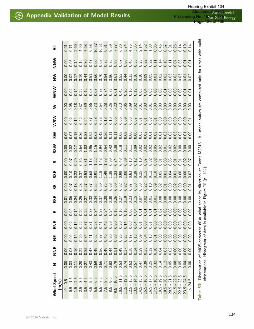
Appendix Validation of Model ResultsRush Creek II
For Xcel Energy
. . . . . . . . . . . . . . . . . . . . . . . . . . . . . . . . . . . . . . . . . . . . . . . . . . . . . . . . . . . . . . . . . . . . . . . . . . . . . . . . . . . . . . . . . . . . . . . . . . . . . . . . . . . . . . . . . .
Win
dSpee
dN
NN
EN
EEN
EE
ESE
SE
SSE
SSSW
SW
WSW
WW
NW
NW
NN
WA
ll(m
/s)
0-
0.5
0.00
0.00
0.00
0.00
0.00
0.01
0.00
0.00
0.00
0.00
0.00
0.00
0.00
0.00
0.00
0.00
0.01
0.5
-1.
50.
030.
030.
040.
020.
040.
060.
070.
100.
070.
020.
070.
020.
050.
020.
020.
050.
711.
5-
2.5
0.11
0.10
0.14
0.14
0.14
0.24
0.13
0.22
0.29
0.17
0.15
0.14
0.18
0.14
0.17
0.14
2.60
2.5
-3.
50.
200.
220.
200.
220.
260.
250.
230.
370.
560.
640.
360.
420.
370.
220.
190.
194.
903.
5-
4.5
0.27
0.35
0.34
0.37
0.22
0.27
0.27
0.53
0.81
1.02
0.83
0.64
0.59
0.42
0.44
0.30
7.68
4.5
-5.
50.
430.
470.
410.
310.
380.
320.
370.
681.
130.
960.
920.
870.
660.
680.
510.
479.
585.
5-
6.5
0.69
0.49
0.62
0.23
0.34
0.34
0.55
0.91
1.22
1.15
0.63
0.58
0.73
0.68
0.60
0.60
10.3
76.
5-
7.5
0.66
0.56
0.37
0.41
0.38
0.37
0.69
1.18
1.43
0.94
0.42
0.33
0.64
0.73
0.70
0.68
10.5
17.
5-
8.5
0.71
0.49
0.46
0.42
0.34
0.28
0.75
1.49
1.33
0.54
0.30
0.18
0.28
0.74
0.84
0.75
9.91
8.5
-9.
50.
820.
440.
300.
290.
240.
300.
681.
380.
990.
420.
110.
100.
250.
720.
800.
758.
599.
5-
10.5
0.79
0.51
0.29
0.20
0.19
0.26
0.69
1.23
0.74
0.38
0.11
0.06
0.20
0.61
0.61
0.88
7.77
10.5
-11
.50.
530.
490.
260.
200.
100.
270.
820.
980.
480.
180.
080.
060.
100.
450.
530.
676.
2011
.5-
12.5
0.74
0.37
0.25
0.14
0.10
0.19
0.92
1.00
0.39
0.11
0.09
0.09
0.06
0.26
0.44
0.60
5.74
12.5
-13
.50.
620.
380.
170.
080.
060.
230.
970.
830.
180.
110.
060.
030.
090.
160.
330.
454.
7513
.5-
14.5
0.57
0.34
0.13
0.04
0.04
0.15
0.68
0.39
0.12
0.09
0.06
0.07
0.02
0.12
0.18
0.35
3.35
14.5
-15
.50.
470.
290.
090.
010.
010.
070.
380.
250.
100.
020.
030.
010.
010.
050.
100.
252.
1415
.5-
16.5
0.39
0.25
0.04
0.00
0.01
0.02
0.22
0.15
0.07
0.02
0.02
0.01
0.00
0.04
0.09
0.22
1.52
16.5
-17
.50.
250.
120.
100.
010.
010.
010.
100.
120.
020.
020.
010.
020.
010.
030.
050.
221.
0817
.5-
18.5
0.32
0.10
0.01
0.00
0.01
0.01
0.09
0.10
0.02
0.05
0.02
0.01
0.00
0.00
0.01
0.11
0.85
18.5
-19
.50.
140.
040.
000.
000.
020.
000.
020.
050.
010.
020.
010.
000.
000.
000.
020.
140.
4519
.5-
20.5
0.12
0.03
0.00
0.00
0.00
0.00
0.01
0.01
0.03
0.01
0.03
0.00
0.00
0.01
0.02
0.10
0.37
20.5
-21
.50.
050.
020.
000.
000.
000.
000.
000.
040.
030.
020.
020.
000.
000.
000.
030.
110.
3121
.5-
22.5
0.08
0.00
0.00
0.00
0.00
0.00
0.02
0.01
0.01
0.02
0.03
0.00
0.00
0.00
0.02
0.07
0.25
22.5
-23
.50.
050.
000.
000.
000.
000.
000.
000.
000.
010.
000.
020.
000.
000.
000.
030.
030.
1423
.5-
24.5
0.04
0.00
0.00
0.00
0.00
0.00
0.00
0.00
0.02
0.00
0.01
0.00
0.00
0.01
0.01
0.01
0.10
>24
.50.
000.
000.
000.
000.
000.
000.
010.
020.
070.
000.
000.
010.
000.
010.
020.
010.
14
Table
53:
Distr
ibution
ofM
OS-c
orre
cted
60m
win
dsp
eed
bydirec
tion
atTow
erM
2313
.A
llm
odel
valu
esar
eco
mpute
don
lyfo
rtim
esw
ith
valid
obse
rvat
ions.
Histo
gram
ofdat
ais
avai
lable
inFig
ure
70(p
.12
4).
c© 2016 Vaisala, Inc.134
Hearing Exhibit 104 Attachment MH-2
Proceeding No. 16A-0117E Page 136 of 138

Appendix Validation of Model ResultsRush Creek II
For Xcel Energy
. . . . . . . . . . . . . . . . . . . . . . . . . . . . . . . . . . . . . . . . . . . . . . . . . . . . . . . . . . . . . . . . . . . . . . . . . . . . . . . . . . . . . . . . . . . . . . . . . . . . . . . . . . . . . . . . . .
Sector Mean Speed(m/s) Weibull Scale(A) Weibull Shape(k) Frequency(%)
N 11.34 12.77 2.56 9.14NNE 9.09 10.26 2.24 5.57NE 7.75 8.73 2.55 5.84ENE 6.85 7.73 2.36 2.80E 6.95 7.83 2.42 2.50
ESE 8.81 9.93 2.53 3.89SE 9.69 10.87 2.92 9.57SSE 8.73 9.82 2.69 11.33S 7.43 8.38 2.41 10.43
SSW 6.83 7.71 2.25 7.26SW 6.72 7.59 2.15 5.69
WSW 6.13 6.90 2.53 4.37W 6.03 6.79 2.57 3.64
WNW 7.28 8.22 2.25 4.51NW 8.76 9.90 2.22 4.99
NNW 10.53 11.87 2.44 8.46
ALL 8.54 9.64 2.25 100.00
Table 54: Observed 60 m mean wind speed, Weibull parameters, and frequency at Tower M2313. Blank values correspondto times with less than 10 data points. Wind rose of data is available in Figure 71 (p. 125).
Sector Mean Speed(m/s) Weibull Scale(A) Weibull Shape(k) Frequency(%)
N 10.75 12.11 2.53 9.09NNE 9.51 10.72 2.45 6.09NE 7.98 9.00 2.35 4.21ENE 7.07 7.97 2.51 3.11E 6.86 7.75 2.30 2.89
ESE 7.72 8.71 2.20 3.66SE 10.01 11.22 2.95 8.67SSE 9.07 10.20 2.71 12.03S 7.61 8.59 2.15 10.14
SSW 6.61 7.46 2.22 6.88SW 6.37 7.17 1.81 4.39
WSW 5.85 6.60 2.11 3.64W 6.14 6.92 2.51 4.22
WNW 7.86 8.84 2.64 6.11NW 8.70 9.82 2.43 6.74
NNW 10.09 11.38 2.40 8.15
ALL 8.56 9.66 2.25 100.00
Table 55: MOS-corrected 60 m mean wind speed, Weibull parameters, and frequency at Tower M2313. All MOS-correctedmodel values are computed only for times with valid observations; blank values correspond to times with lessthan 10 data points. Wind rose of data is available in Figure 71 (p. 125).
c© 2016 Vaisala, Inc.135
Hearing Exhibit 104 Attachment MH-2
Proceeding No. 16A-0117E Page 137 of 138
ReferencesRush Creek II
For Xcel Energy
. . . . . . . . . . . . . . . . . . . . . . . . . . . . . . . . . . . . . . . . . . . . . . . . . . . . . . . . . . . . . . . . . . . . . . . . . . . . . . . . . . . . . . . . . . . . . . . . . . . . . . . . . . . . . . . . . .
REFERENCES. . . . . . . . . . . . . . . . . . . . . . . . . . . . . . . . . . . . . . . . . . . . . . . . . . . . . . . . . . . . . . . . . . . . . . . . . . . . . . . . . . . . . . . . . . . . . . . . . . . . . . . . . . . . . . . . . . . . . . . . . . . . . . . . . . . . . . . .
[1] K.J. Allwine and C.D. Whiteman. MELSAR: A mesoscale air quality model for complex terrain: Volume 1–overview,technical description and user’s guide. Technical report, Pacific Northwest National Laboratory, 1985.
[2] O. Arino, P. Bicheron, F. Achard, J. Latham, R. Witt, and J.L. Weber. Globcover: The most detailed portrait ofearth. ESA Bulletin, 136, 2008.
[3] D. P. Dee, S. M. Uppala, A. J. Simmons, P. Berrisford, P. Poli, S. Kobayashi, U. Andrae, M. A. Balmaseda, G. Balsamo,P. Bauer, P. Bechtold, A. C. M. Beljaars, L. van de Berg, J. Bidlot, N. Bormann, C. Delsol, R. Dragani, M. Fuentes,A. J. Geer, L. Haimberger, S. B. Healy, H. Hersbach, E. V. Holm, L. Isaksen, P. Kallberg, M. Kohler, M. Matricardi,A. P. McNally, B. M. Monge-Sanz, J.-J. Morcrette, B.-K. Park, C. Peubey, P. de Rosnay, C. Tavolato, J.-N. Thepaut,and F. Vitart. The era-interim reanalysis: Configuration and performance of the data assimilation system. Quart. J.Roy. Meteor. Soc., 137:553—-597, 2011.
[4] A. Jarvis et al. Hole-filled seamless SRTM data V4. International Centre for Tropical Agriculture (CIAT), availablefrom http://srtm.csi.cgiar.org, 2008.
[5] E. Kalnay, M. Kanamitsu, R. Kistler, W. Collins, D. Deaven, L. Gandin, M. Iredell, S. Saha, G. White, J. Woollen,Y. Zhu, M. Chelliah, W. Ebisuzaki, W.Higgins, J. Janowiak, K. C. Mo, C. Ropelewski, J. Wang, A. Leetmaa,R. Reynolds, Roy Jenne, and Dennis Joseph. The NCEP/NCAR 40-year reanalysis project. Bull. Amer. Meteor.Soc., 77:437–470, 1996.
[6] G.C. Larsen, Jørgen Højstrup, and H. A. Madsen. Wind fields in wakes. In Proceedings EWEC 1996, pages 764–768,Goteborg, Sweden, 1996.
[7] M.K. Liu and M.A. Yocke. Siting of wind turbine generators in complex terrain. Journal of Energy, 4:10–16, 1980.
[8] M.M. Rienecker, M.J. Suarez, R. Gelaro, R. Todling, J. Bacmeister, E. Liu, M.G. Bosilovich, S.D. Schubert, L. Takacs,G.K. Kim, S. Bloom, J. Chen, D. Collins, A. Conaty, and A. da Silva. Merra: Nasa’s modern-era retrospective analysisfor research and applications. J. Climate, 24:3624–3648, 2011.
[9] T. Sorensen, P. Nielsen, and M. L. Thøgersen. Recalibrating wind turbine wake model parameters - validating thewake model performance for large offshore wind farms. In Proceedings EWEC 2006, Athens, Greece, 2006.
c© 2016 Vaisala, Inc.136
Hearing Exhibit 104 Attachment MH-2
Proceeding No. 16A-0117E Page 138 of 138