Embed Size (px)
Citation preview
Duality
▶ Lagrange dual problem
▶ weak and strong duality
▶ optimality conditions
▶ perturbation and sensitivity analysis
▶ generalized inequalities
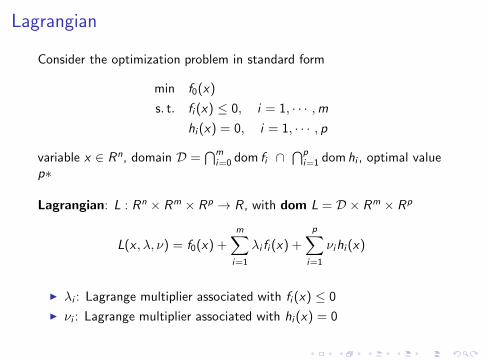
Lagrangian
Consider the optimization problem in standard form
min f0(x)
s. t. fi (x) ≤ 0, i = 1, ⋅ ⋅ ⋅ ,m
hi (x) = 0, i = 1, ⋅ ⋅ ⋅ , p
variable x ∈ Rn, domain D =∩m
i=0dom fi ∩
∩p
i=1dom hi , optimal value
p∗
Lagrangian: L : Rn × Rm × Rp → R , with dom L = D × Rm × Rp
L(x , �, �) = f0(x) +m∑
i=1
�i fi (x) +
p∑
i=1
�ihi (x)
▶ �i : Lagrange multiplier associated with fi (x) ≤ 0
▶ �i : Lagrange multiplier associated with hi (x) = 0

Lagrangian dual function
Lagrangian dual function: g : Rm × Rp → R ,
g(�, �) = infx∈D
L(x , �, �)
= infx∈D
f0(x) +
m∑
i=1
�i fi (x) +
p∑
i=1
�ihi (x)
g is concave, can be −∞ for some �, �
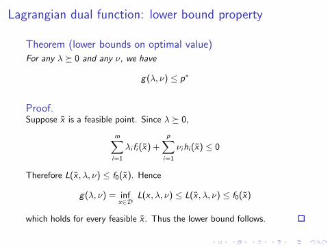
Lagrangian dual function: lower bound property
Theorem (lower bounds on optimal value)For any � ર 0 and any �, we have
g(�, �) ≤ p∗
Proof.Suppose x̃ is a feasible point. Since � ર 0,
m∑
i=1
�i fi (x̃) +
p∑
i=1
�ihi(x̃) ≤ 0
Therefore L(x̃ , �, �) ≤ f0(x̃). Hence
g(�, �) = infx∈D
L(x , �, �) ≤ L(x̃ , �, �) ≤ f0(x̃)
which holds for every feasible x̃ . Thus the lower bound follows.

The dual problem
Lagrange dual problem
max g(�, �)
s. t. � ર 0
▶ find the best lower bound on p∗
▶ a convex optimization problem; optimal value denoted d∗
▶ �, � are dual feasible if � ર 0, (�, �) ∈ dom g (meansg(�, �) > −∞)
▶ (�∗, �∗): dual optimal multipliers
▶ p∗ − d∗ is called the optimal duality gap

Weak and strong duality
Weak duality: d∗ ≤ p∗
▶ always true (for both convex and nonconvex problems)
Strong duality: d∗ = p∗
▶ does not hold in general
▶ (usually) holds for convex problems
▶ conditions that guarantee strong duality in convex problems arecalled constraint qualifications
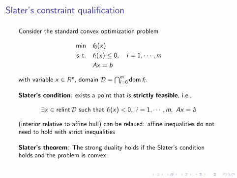
Slater’s constraint qualification
Consider the standard convex optimization problem
min f0(x)
s. t. fi (x) ≤ 0, i = 1, ⋅ ⋅ ⋅ ,m
Ax = b
with variable x ∈ Rn, domain D =∩m
i=0dom fi .
Slater’s condition: exists a point that is strictly feasible, i.e.,
∃x ∈ relintD such that fi (x) < 0, i = 1, ⋅ ⋅ ⋅ ,m, Ax = b
(interior relative to affine hull) can be relaxed: affine inequalities do notneed to hold with strict inequalities
Slater’s theorem: The strong duality holds if the Slater’s conditionholds and the problem is convex.
Complementary slackness
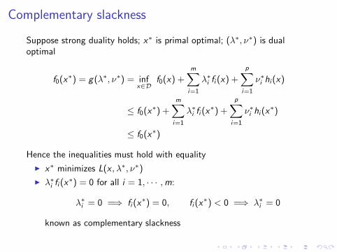
Suppose strong duality holds; x∗ is primal optimal; (�∗, �∗) is dualoptimal
f0(x∗) = g(�∗, �∗) = inf
x∈Df0(x) +
m∑
i=1
�∗i fi (x) +
p∑
i=1
�∗i hi(x)
≤ f0(x∗) +
m∑
i=1
�∗i fi (x
∗) +
p∑
i=1
�∗i hi(x∗)
≤ f0(x∗)
Hence the inequalities must hold with equality
▶ x∗ minimizes L(x , �∗, �∗)
▶ �∗i fi (x
∗) = 0 for all i = 1, ⋅ ⋅ ⋅ ,m:
�∗i = 0 =⇒ fi (x
∗) = 0, fi (x∗) < 0 =⇒ �∗
i = 0
known as complementary slackness
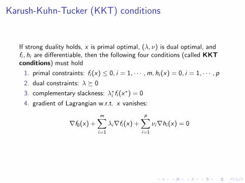
Karush-Kuhn-Tucker (KKT) conditions
If strong duality holds, x is primal optimal, (�, �) is dual optimal, andfi , hi are differentiable, then the following four conditions (called KKT
conditions) must hold
1. primal constraints: fi (x) ≤ 0, i = 1, ⋅ ⋅ ⋅ ,m, hi (x) = 0, i = 1, ⋅ ⋅ ⋅ , p
2. dual constraints: � ર 0
3. complementary slackness: �∗i fi (x
∗) = 0
4. gradient of Lagrangian w.r.t. x vanishes:
∇f0(x) +
m∑
i=1
�i∇fi (x) +
p∑
i=1
�i∇hi(x) = 0

KKT conditions for convex problem
If x̃ , �̃, �̃ satisfy KKT for a convex problem, then they are optimal:
▶ from complementary slackness: f0(x̃) = L(x̃ , �̃, �̃)
▶ from the 4-th condition and convexity: g(�̃, �̃) = L(x̃ , �̃, �̃)
So f0(x̃) = g(�̃, �̃)
If the Slater’s condition is satisfied and fi is differentiable, then x isoptimal iff ∃�, � that satisfy KKT
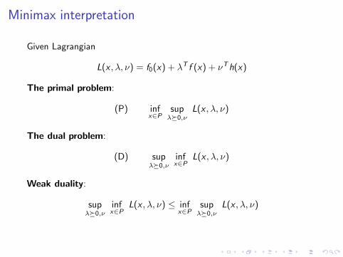
Minimax interpretation
Given Lagrangian
L(x , �, �) = f0(x) + �T f (x) + �Th(x)
The primal problem:
(P) infx∈P
sup�ર0,�
L(x , �, �)
The dual problem:
(D) sup�ર0,�
infx∈P
L(x , �, �)
Weak duality:
sup�ર0,�
infx∈P
L(x , �, �) ≤ infx∈P
sup�ર0,�
L(x , �, �)
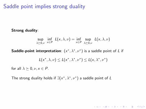
Saddle point implies strong duality
Strong duality:
sup�ર0,�
infx∈P
L(x , �, �) = infx∈P
sup�ર0,�
L(x , �, �)
Saddle-point interpretation: (x∗, �∗, �∗) is a saddle point of L if
L(x∗, �, �) ≤ L(x∗, �∗, �∗) ≤ L(x , �∗, �∗)
for all � ર 0, �, x ∈ P .
The strong duality holds if ∃(x∗, �∗, �∗) a saddle point of L

Examples
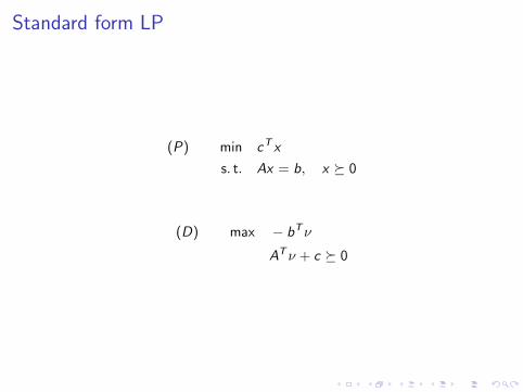
Standard form LP
(P) min cT x
s. t. Ax = b, x ર 0
(D) max − bT�
AT � + c ર 0
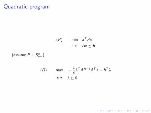
Quadratic program
(P) min xTPx
s. t. Ax ⪯ b
(assume P ∈ Sn++)
(D) max −1
4�TAP−1AT�− bT�
s. t. � ર 0
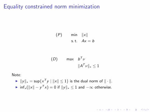
Equality constrained norm minimization
(P) min ∥x∥
s. t. Ax = b
(D) max bT�
∥AT�∥∗ ≤ 1
Note:
▶ ∥y∥∗ = sup{xTy ∣ ∥x∥ ≤ 1} is the dual norm of ∥ ⋅ ∥.
▶ infx(∥x∥ − yT x) = 0 if ∥y∥∗ ≤ 1 and −∞ otherwise.
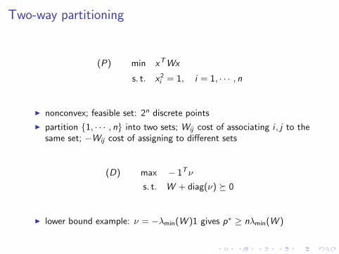
Two-way partitioning
(P) min xTWx
s. t. x2i = 1, i = 1, ⋅ ⋅ ⋅ , n
▶ nonconvex; feasible set: 2n discrete points
▶ partition {1, ⋅ ⋅ ⋅ , n} into two sets; Wij cost of associating i , j to thesame set; −Wij cost of assigning to different sets
(D) max − 1T�
s. t. W + diag(�) ર 0
▶ lower bound example: � = −�min(W )1 gives p∗ ≥ n�min(W )

Perturbation and sensitivity anaysis
perturbed optimization problem
min f0(x)
s. t. fi (x) ≤ ui , i = 1, ⋅ ⋅ ⋅ ,m
hi (x) = vi , i = 1, ⋅ ⋅ ⋅ , p
its dual
min g(�, �)− uT�− vT�
s. t. � ર 0
▶ x primal variable; u, v are parameters
▶ p∗(u, v) is optimal value as a function of u, v
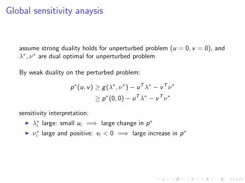
Global sensitivity anaysis
assume strong duality holds for unperturbed problem (u = 0, v = 0), and�∗, �∗ are dual optimal for unperturbed problem
By weak duality on the perturbed problem:
p∗(u, v) ≥ g(�∗, �∗)− uT�∗ − vT �∗
≥ p∗(0, 0)− uT�∗ − vT �∗
sensitivity interpretation:
▶ �∗i large: small ui =⇒ large change in p∗
▶ �∗i large and positive: vi < 0 =⇒ large increase in p∗
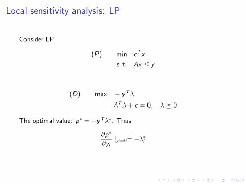
Local sensitivity analysis: LP
Consider LP
(P) min cT x
s. t. Ax ≤ y
(D) max − yT�
AT�+ c = 0, � ર 0
The optimal value: p∗ = −yT�∗. Thus
∂p∗
∂yi∣yi=0= −�∗
i

Local sensitivity analysis
Suppose strong duality holds for unperturbed problem (u = 0, v = 0),and �∗, �∗ are dual optimal for unperturbed problem. If p∗(u, v) isdifferentiable at (0, 0), then
�∗i = −
∂p∗(0, 0)
∂ui�∗i = −
∂p∗(0, 0)
∂vi
If p∗(u, v) is not differentiable at (0, 0), then (−�∗,−�∗) ∈ ∂p∗(0, 0).
Proof.By the weak duality on the perturbed problem:
∂p∗(0, 0)
∂ui= lim
t↓0
p∗(tei , 0)− p∗(0, 0)
t≥ −�∗
i
∂p∗(0, 0)
∂ui= lim
t↑0
p∗(tei , 0)− p∗(0, 0)
t≤ −�∗
i
Thus equality holds. Similar proof for �∗i

Problems with generalized inequalities
min f0(x)
s. t. fi (x) રKi0, i = 1, ⋅ ⋅ ⋅ ,m
hi(x) = vi , i = 1, ⋅ ⋅ ⋅ , p
Lagrangian
▶ �i : Lagrange multiplier for fi(x) ≤Ki0
▶ Lagrangian L:
L(x , �1, ⋅ ⋅ ⋅ , �m, �) = f0(x) +
m∑
i=1
�Ti fi (x) +
p∑
i=1
�ihi (x)
▶ Dual function g :
g(�1, ⋅ ⋅ ⋅ , �m, �) = infx∈D
L(x , �1, ⋅ ⋅ ⋅ , �m, �, x)
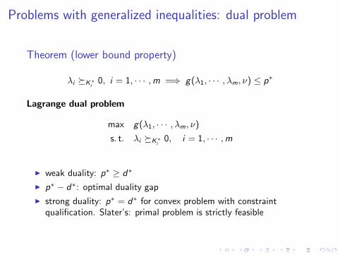
Problems with generalized inequalities: dual problem
Theorem (lower bound property)
�i રK∗
i0, i = 1, ⋅ ⋅ ⋅ ,m =⇒ g(�1, ⋅ ⋅ ⋅ , �m, �) ≤ p∗
Lagrange dual problem
max g(�1, ⋅ ⋅ ⋅ , �m, �)
s. t. �i રK∗
i0, i = 1, ⋅ ⋅ ⋅ ,m
▶ weak duality: p∗ ≥ d∗
▶ p∗ − d∗: optimal duality gap
▶ strong duality: p∗ = d∗ for convex problem with constraintqualification. Slater’s: primal problem is strictly feasible
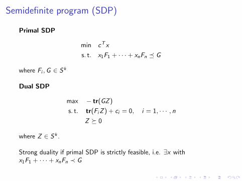
Semidefinite program (SDP)
Primal SDP
min cT x
s. t. x1F1 + ⋅ ⋅ ⋅+ xnFn ⪯ G
where Fi ,G ∈ Sk
Dual SDP
max − tr(GZ )
s. t. tr(FiZ ) + ci = 0, i = 1, ⋅ ⋅ ⋅ , n
Z ર 0
where Z ∈ Sk .
Strong duality if primal SDP is strictly feasible, i.e. ∃x withx1F1 + ⋅ ⋅ ⋅+ xnFn ≺ G


![arXiv:1606.05058v1 [math.CT] 16 Jun 2016arXiv:1606.05058v1 [math.CT] 16 Jun 2016 CONTRAVARIANCE THROUGH ENRICHMENT MICHAEL SHULMAN Abstract. We define strict and weak duality involutions](https://img.pdfslide.us/doc/110x75/5e76dbec250b1b73bb53916c/arxiv160605058v1-mathct-16-jun-2016-arxiv160605058v1-mathct-16-jun-2016.jpg)