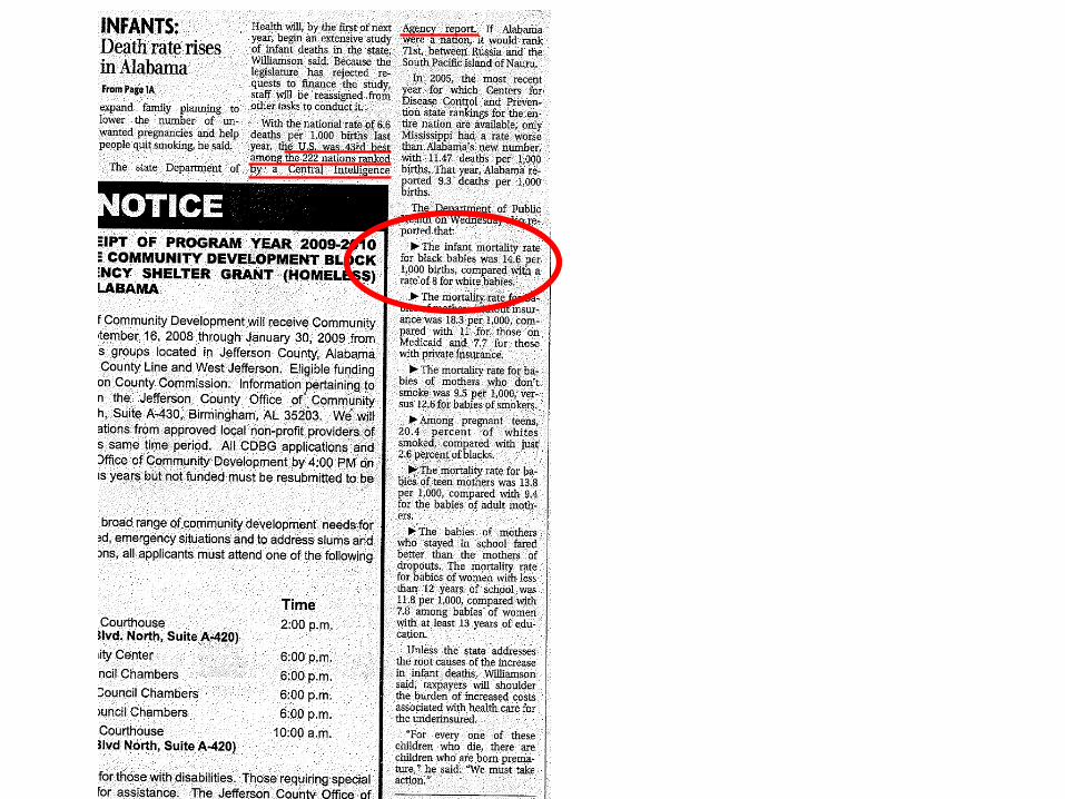
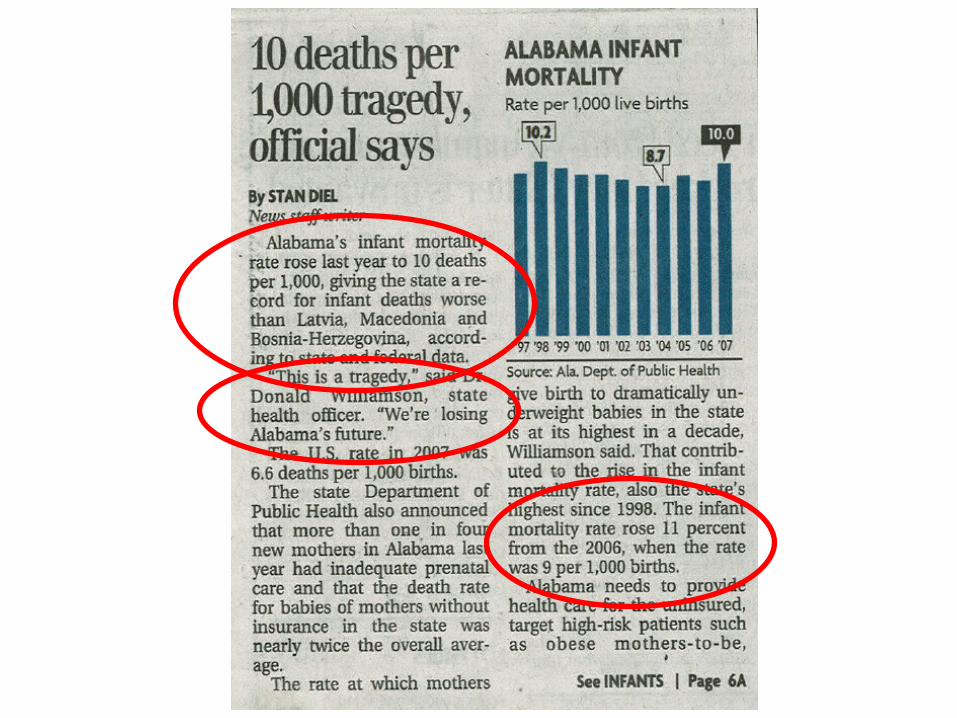
Dual Tragedies in the B-ham Paper

Module 2Simple Descriptive Statistics and

Univariate Displays of Data

A Tale of Three Cities

George Howard, DrPH

A Tale of Three CitiesBackground

• There were substantial differences in cancer rates between regions of Alabama– Birmingham 143/100,000

– Mobile 110/100,000

– Montgomery 94/100,000

• Could these differences be due to the horrible air pollution largely caused by highway 280 in Birmingham?

• The suspect agent is suspended particulate matter

A Tale of Three CitiesCollection of Data

• Sampled suspended particulate matter (ppm) in the three cities on randomly selected days.

• What are the patterns here?

• What are the differences between these cities?

• Describe the variables in this analysis

Birmingham (n=15)150131136149126141122135110123 87116128130127

Mobile (n=25)139160126168140142211152170103170141139121178165123178219131174112160168162

Montgomery (n=28) 113 155 100 94 146 111 145 92 173 100 105 110 106 114 136 151 98 94 118 137 123 159 96 128 127 120 80 230

 

 

Type of Independent Data

Categorical Continuous

Two Samples Multiple Samples

Type of Dependent Data

OneSample(focususually onestimation) Independent Matched Independent

RepeatedMeasures Single Multiple

Categorical (dichotomous) 1Estimateproportion(andconfidencelimits)

2Chi-SquareTest

3McNemarTest

4 Chi SquareTest

5GeneralizedEstimatingEquations(GEE)

6LogisticRegression

7LogisticRegression

Continuous 8Estimatemean (andconfidencelimit)

9Independent t-test

10Paired t-test

11Analysis ofVariance

12MultivariateAnalysis ofVariance

13Simple linearregression &correlationcoefficient

14MultipleRegression

Right Censored (survival) 15KaplanMeierSurvival

16Kaplan MeierSurvival forboth curves,with tests ofdifference byWilcoxon orlog-rank test

17Veryunusual

18Kaplan-MeierSurvival foreach group,with tests bygeneralizedWilcoxon orGeneralizedLog Rank

19Veryunusual

20ProportionalHazardsanalysis

21ProportionalHazardsanalysis

Types of Statistical Tests and Approaches

Consider the Birmingham Data

• Place the data in equally spaced categoriesInterval Mid # %

82.5<X<97.5 90 1 6.7

97.5<X<112.5 105 1 6.7

112.5<X<127.5 120 5 33.3

127.5<X<142.5 135 6 40.0

142.5<X<157.5 150 2 13.3

• Clustering of points around 112-142 categories, with fewer points on either side

Birmingham (n=15)150131136149126141122135110123 87116128130127

A Tale of Three CitiesDescription of Birmingham SPM

Birmingham

01234567

90 105 120 135 150

SPM (ppm)

Fre

quen

cy

A Tale of Three CitiesDescription of Birmingham SPM

• How do you choose how many intervals to have in a histogram?– Rule of thumb: 3+ observations per category

• Remember where you make the cutpoints is also an arbitrary decision --- that changes how the histogram looks

Birmingham

01234567

90 105 120 135 150

SPM (ppm)

Fre

quen

cy

Birmingham

0

1

2

3

4

5

6

90 100 110 120 130 140 150

SPM (ppm)

Fre

quen

cy

Birmingham

01234567

90 105 120 135 150

SPM (ppm)

Fre

qu

ency

Montgomery

02468

10121416

75 105 135 165 195 225

SPM (ppm)

Fre

qu

ency

Mobile

0

2

4

6

8

10

12

113 138 163 188 213

SPM (ppm)

Fre

qu

ency

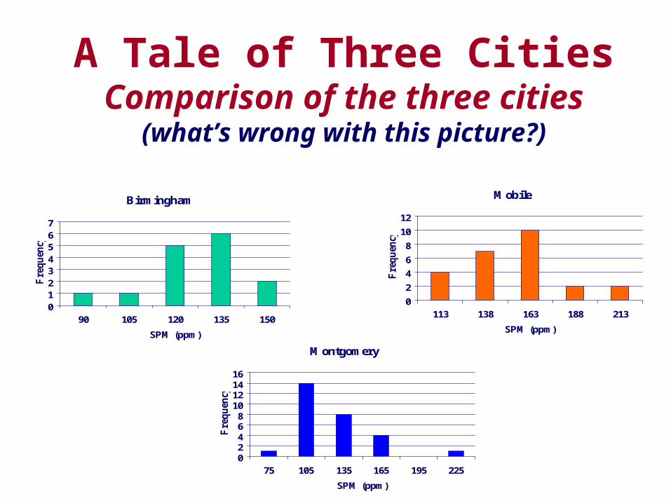
A Tale of Three CitiesComparison of the three cities

(what’s wrong with this picture?)

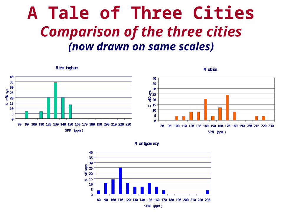
A Tale of Three CitiesComparison of the three cities

(now drawn on same scales)

Birmingham

0

5

10

15

20

25

30

35

40

80 90 100 110 120 130 140 150 160 170 180 190 200 210 220 230

SPM (ppm)

% o

f Day

s

Mobile

0

5

10

15

20

25

30

35

40

80 90 100 110 120 130 140 150 160 170 180 190 200 210 220 230

SPM (ppm)

% o

f Day

s

Montgomery

0

5

10

15

20

25

30

35

40

80 90 100 110 120 130 140 150 160 170 180 190 200 210 220 230

SPM (ppm)

% o

f Day

s

How do we describe these cities with a few simple numbers?

• Where is the middle of the data (that is an “average” value)?

• How spread out are the numbers?

• Are there other measures that may be important to describe these data?

Gee, what do we mean by “average” anyway

• Measures of “central tendency”

• There are MANY ways to calculate an average

• Two most common ways– The arithmetic mean– The median

• There are other approaches

The Arithmetic Mean

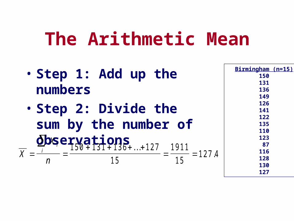
• Step 1: Add up the numbers

• Step 2: Divide the sum by the number of observations

Birmingham (n=15)150131136149126141122135110123 87116128130127

XX

n

ii

1 5 0 1 3 1 1 3 6 1 2 7

1 5

1 9 11

1 51 2 7 4

. . ..

The Median

• The point where half the data are bigger (and half less)

• There are at least 4 rules to find the median (and other percentiles)

• The rules differ if there are an odd or even number of data points– If odd, then the “middle” data point– If even, then the average of the “two middle” data

points

The Median(continued)

• Step 1: Sort the data

• Step 2: Pick the median

• Consider Birmingham data (note that there are an odd number of data points)

• Median is 128

Birmingham (n=15) 87110116122123126127

8th of 15 data points==> 128130131135136141149150

The Median(continued)

• Suppose we only had 14 data points in Birmingham

• Step 1: Find the middle two data points

• Step 2: Take the average difference between these two observations

• Median = 127.5

Birmingham (n=now with 14 points) 87110116122123126

7th of 14 data points==> 127 8th of 14 data points==> 128

130131135136141149

A Tale of Three CitiesMeasures of Central Tendency

Birmingham

0

5

10

15

20

25

30

35

40

80 90 100 110 120 130 140 150 160 170 180 190 200 210 220 230

SPM (ppm)

% o

f Day

s

Mobile

0

5

10

15

20

25

30

35

40

80 90 100 110 120 130 140 150 160 170 180 190 200 210 220 230

SPM (ppm)

% o

f Day

s

Montgomery

0

5

10

15

20

25

30

35

40

80 90 100 110 120 130 140 150 160 170 180 190 200 210 220 230

SPM (ppm)

% o

f Day

s

Mean = 127.4Median = 128

Mean = 154.0Median = 154

Mean = 123.6Median = 116

Measures of Central Tendency

• Birmingham and Montgomery have lower measures of central tendency than Mobile

• For Birmingham and Mobile, the mean and median are almost the same value– This happens when distributions are symmetric

• For Montgomery, the mean is quite a bit higher than the median– The mean is “pulled up” by outliers

– The median is not sensitive to outliers

How “spread out” are the measures

• Measures of “dispersion”• The range is the most simple measure

– Birmingham: 150 - 87 = 63– Mobile: 219 - 103 = 116– Montgomery: 230 - 80 = 150

• It appears that data from Montgomery are very spread out, Mobile is not as spread out, and Birmingham is very “compact”

• Range is influenced by the outliers

How “spread out” are the measures (continued)

• The range is influenced by outliers (just like the mean) --- – But the median is not influenced by the

outliers– Is there some measure of dispersion that will

not be so affected by 1 (or 2) points

Measures of DispersionPercentiles

• The kth percentile is that place in the data where k-% of the data are below the cutpoint

• There are many alternative approaches to define percentiles

• In one approach, they are determined by the function k*(n+1)– If integer, then pick that data point

– If non-integer, then average the two data points around that point

Measures of DispersionPercentiles (continued)

• For example, consider the 25%-tile from Birmingham– Step 1: calculate k*(n+1) = 0.25*(15+1) = 4– Step 2: since this is integer, then pick the 4th data

point– 25%-tile is 122

• Consider the 33%tile from Birmingham– Step 1: calculate k*(n+1) = 0.33*(15+1) = 5.3– Step 2: average the 5th and 6th data points– 33%-tile is 1/2 way between 123 and 126 or 124.5

Birmingham (n=15) 87110116122123126127128130131135136141149

Percentiles from the 3 Cities

Birmingham Mobile Montgomery

10th 110 121 94

25th 122 139 100

50th 128 160 116

75th 136 170 141

90th 150 178 159

Measures of DispersionPercentiles (continued)

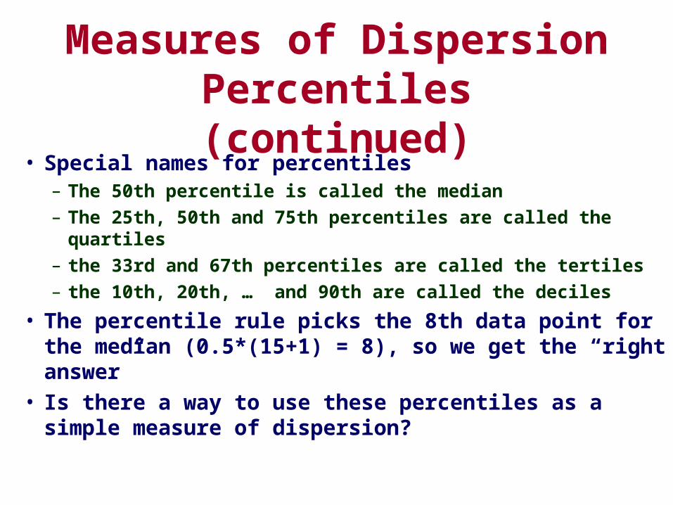
• Special names for percentiles– The 50th percentile is called the median

– The 25th, 50th and 75th percentiles are called the quartiles

– the 33rd and 67th percentiles are called the tertiles

– the 10th, 20th, … and 90th are called the deciles

• The percentile rule picks the 8th data point for the median (0.5*(15+1) = 8), so we get the “right answer”

• Is there a way to use these percentiles as a simple measure of dispersion?

Percentiles from the 3 CitiesBirmingham Mobile Montgomery

10th 110 121 94

25th 122 139 100

50th 128 160 116

75th 136 170 141

90th 150 178 159

InterquartileRange

136 – 122= 14

170 – 139= 31

141 – 100= 41

Interdecilerange

150 – 110= 40

178 – 121= 57

159 – 94= 65

Percentiles from the 3 Cities

• Percentiles are relatively insensitive to “outliers”

• How do we define outliers– Rule of thumb --- If a data point is an “outlier”

• Above 1.5 interquartile ranges over the 75th percentile

• Below 1.5 interquartile ranges under the 25th percentile

– Consider Montgomery data• Interquartile range is 41

• 75th percentile is 141

• Outliers are above 141+1.5*41=202.5

• The value at 230 is an “outlier”

Percentiles from the 3 Cities

• So, percentiles are “neat”– But with even 3 cities we have to think about

21 or more numbers • 10th, 25th, 50th, 75th, 90th, percentiles

• interquartile range, interdecile range

• Isn’t there some way to look at these graphically and to see the outliers

• Box and whisker plots

Percentiles from the 3 Cities Box and Whisker Plots

• Draw box– Top of box is the 75th-ptile (136)– Bottom of box is 25th- ptile (122)– Line is 50th ptile (median=128)

• Find outliers– Below 122-1.5*14=101– Above 136+1.5*14= 157– Plot outlier(s) as a point (87)

• Draw “whiskers” to the the highest non-outlier (149) and lowest non-outlier (110) points

• Plot outliers as single data points

15N =

SPM

160

150

140

130

120

110

100

90

80

11

Birmingham (n=15) 87110116122123126127128130131135136141149

Percentiles from the 3 Cities Box and Whisker Plots

• Box and Whisker plots make for easy comparison of groups– B-ham doesn’t have

much spread

– Mobile is considerably above B-ham or Montgomery

– B-ham and Mobile are fairly symmetric

282515N =

City

MontgomeryMobileBirmingham

SP

M

300

200

100

0

6834

11

Measures of DispersionStandard Deviation (and Variance)

• So far we have two measures of dispersion– Range

– Percentiles (and differences between percentiles)

• Is there another single number that summarizes how spread out the data are?

• Consider measures of how far the data are from the mean– If data are far from the mean, then they are really spread out

– This is the idea for the Standard Deviation

Measures of DispersionStandard Deviation (and Variance)

• Idea #1 (a logical but dumb one)– Calculate the average distance each data

point is from the mean (absolute value)– Take the average of these numbers– Mean absolute deviation

MADX X

ni

i

| |

| . | | . | . . . | . | . . . . . . ..

1 27 4 8 7 1 27 4 11 0 1 27 4 1 49

1 5

4 0 4 1 4 4 2 1 6

1 5

1 61 6

1 51 0 8

• Idea #2 (a great one --- although it seems illogical)

• Take the square root of the sum of the squared deviations divided by the n-1

Measures of DispersionStandard Deviation (and Variance)

SDX X

ni

i

( )

( . ) ( . ) . . . ( . ) . . ..

22 2 2

1

1 2 7 4 8 7 1 2 7 4 11 0 1 2 7 4 1 4 9

1 5 1

1 6 3 2 3 0 3 5 11

1 4

3 4 3 0

1 41 5 6

• The variance is the standard deviation squared (15.6)2=245.0

A Tale of Three CitiesDescriptive Statistics

Birmingham

0

5

10

15

20

25

30

35

40

80 90 100 110 120 130 140 150 160 170 180 190 200 210 220 230

SPM (ppm)

% o

f Day

s

Mobile

0

5

10

15

20

25

30

35

40

80 90 100 110 120 130 140 150 160 170 180 190 200 210 220 230

SPM (ppm)

% o

f Day

s

Montgomery

0

5

10

15

20

25

30

35

40

80 90 100 110 120 130 140 150 160 170 180 190 200 210 220 230

SPM (ppm)

% o

f Day

s

Mean = 127.4Median = 128Range = 63IQR = 14SD = 15.6

Mean = 154.0Median = 154Range = 116IQR = 31SD = 28.0

Mean = 123.6Median = 116Range = 150IQR = 41SD = 31.3

Summary: Descriptive Statistics and Simple Graphs

• What we have talked about– Histogram

– Measures of Central Tendency• Mean• Median

– Measures of Dispersion• Range• Percentiles

– Interquartile range

– Interdecile range

• Standard deviation

– Box and Whisker plots

Summary: Descriptive Statistics and Simple Graphs

• What we have not talked about– Simple descriptive statistics

to describe skew

– Simple descriptive statistics to describe kurtosis

• There are many other kinds of graphs not discussed

NEW

400.0

375.0

350.0

325.0

300.0

275.0

250.0

225.0

200.0

175.0

150.0

125.0

100.0

75.0

50.0

25.0

0.0

10

8

6

4

2

0

Std. Dev = 91.44

Mean = 112.4

N = 50.00

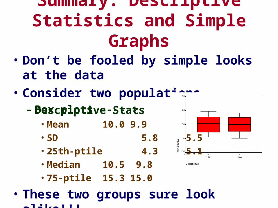
• Don’t be fooled by simple looks at the data

• Consider two populations– Box plots ----->

Summary: Descriptive Statistics and Simple Graphs

4040N =

VAR00001

2.001.00

VA

R0

00

02

30

20

10

0

-10

– Descriptive Stats• Mean 10.0 9.9

• SD 5.8 5.5

• 25th-ptile 4.3 5.1

• Median 10.5 9.8

• 75-ptile 15.3 15.0

• These two groups sure look alike!!!

But --- Here are the two distributions

VAR00002

20.018.016.014.012.010.08.06.04.02.00.0

VAR00001: 1.008

6

4

2

0

Std. Dev = 5.83

Mean = 10.0

N = 40.00

VAR00002

18.016.014.012.010.08.06.04.02.00.0

VAR00001: 2.007

6

5

4

3

2

1

0

Std. Dev = 5.49

Mean = 9.9

N = 40.00

A Tale of 3 CitiesConclusions

• B-ham appeared to have consistently lower levels of SPM than either Mobile or Montgomery– Lower measures of central tendency– Less dispersion

• It would seem hard to argue that high levels of SPM is the cause of the higher cancer rates

Dual Tragedies in the B-ham Paper