Multi-Period Dual Pricing Algorithm for Cost Allocation in Non-Convex Electricity Markets

Robin Broder Hytowitz1,2, Richard P. O’Neill1 and Brent Eldridge1,2

1Federal Energy Regulatory Commission, Washington, DC2Johns Hopkins University, Baltimore, MD

The views expressed are not necessarily those of the Commission. 1

Outline• What makes a good price?

– Price Formation NOPR• Dual Pricing Algorithm

– Basic unit commitment formulation– Alternative pricing formulations– Multi-period DPA model

• Comparison of pricing methods– Examples

2

What makes a good price?• In convex cases, market clearing prices

are– Revenue neutral– Non-confiscatory– Incent investment (signals for entry)

• Electricity markets are non-convex due to lumpy costs

3

pric

e

quantity

demand

supply

Literature• Many proposals for non-convex pricing

– LMP with uplift payments (O’Neill, Sotkiewicz, Hobbs, Rothkopf, Stewart)– Convex hull (Hogan & Ring ; Gribik, Hogan & Pope)– Extended LMP (Wang, Luh, Gribik, Zhang & Peng)– Modified LMP (Bjørndal & Jörnsten)– General uplift with zero-sum transfers (Motto & Galiana)– Semi-Lagrangean approach (Araoz & Jörnsten)– Primal-dual approach (Ruiz, Conejo, & Gabriel)– Review and internal zero-sum uplifts (Liberopoulos & Andrianesis)

4

Two-Part Pricing Single PriceSchweppe

[25]O’Neill

[9]Gribik

[10], [11]ELMP[14]

Bjørndal[6]

Galiana[15], [16]

DPA[4] AIC Araoz

[18]Ruiz[19]

Maximize market surplus Y Y Y Y Y Y Y Y Y NRevenue neutral Y N N N N Y Y Y Y YIncludes demand side Y N N N N Y Y Y Y YMaintain optimal dispatch Y Y Y Y Y Y Y Y Y NTransparency Y N N N N N Y/N Y Y YUplifts Ex-post Ex-post Ex-post Ex-post Ex-post Internal Internal None None NonePricing problem type LP LP CH LP LP+ NLP LP LP LP+ MIP*

FERC Price Formation• What are the goals of price formation?*

– Maximize market surplus– Provide correct incentives for market participants to

follow commitment and dispatch instructions and make efficient investments

– More transparently reflect the marginal cost of serving load and operational constraints

– Ensure suppliers can recover costs

5*Adapted from Order Directing Reports on Price Formation AD14-14-000

Pricing & Cost Allocation Principles

Revenue neutrality• For each market

payments equal receipts• Money out = money in

Maximize surplus• Assumes demand can bid their value

Non-confiscation• Incent participants to stay

in the market• Generator profits ≥ 0• Net demand value ≥ 0

Incentivize efficient investments

• Prices signal entry into the market

• Transparency

6

Pricing Principles

• New pricing system?– Begin with economic principles – Address any deficiencies

7

Current pricing system:LMP Side payment+

Public Private & discriminatory

Ramsey-Boiteux Pricing• Ramsey: allocate fixed costs based on willingness to

pay– Inverse elasticity pricing rule– Discriminatory (but not unduly discriminatory)

• Boiteux: differentiated a public and private price– Demand that is more elastic pays less

• Necessary for efficiency in non-convex markets

8

𝜆𝜆𝑟𝑟 =𝑐𝑐′ 𝑝𝑝

1 − 𝛼𝛼/𝑒𝑒 → 𝜆𝜆𝑟𝑟 = 𝑐𝑐′ 𝑝𝑝 + 𝜆𝜆𝑟𝑟 𝛼𝛼/𝑒𝑒𝑒𝑒 Demand elasticity

𝑐𝑐′(𝑝𝑝) Marginal cost function𝛼𝛼 −𝛾𝛾/(1 − 𝛾𝛾) dual of cost

recovery constraint

Additional considerations• Ease of implementation

– Type of problem: linear, mixed-integer• Incentive for following dispatch

– Penalties administered or opportunity costs paid – Market power mitigated through regulation

• Demand side participation– Demand is price responsive (some markets seeing

higher participation)

9

Post-Unit Commitment Pricing Modelmax ∑𝑡𝑡∈𝑇𝑇 ∑𝑖𝑖∈𝐷𝐷 𝑏𝑏𝑖𝑖𝑡𝑡𝑑𝑑𝑖𝑖𝑡𝑡 − ∑𝑖𝑖∈𝐺𝐺 𝑐𝑐𝑖𝑖𝑡𝑡𝑝𝑝𝑖𝑖𝑡𝑡 + 𝑐𝑐𝑖𝑖𝑡𝑡𝑂𝑂𝑂𝑂𝑢𝑢𝑖𝑖𝑡𝑡 + 𝑐𝑐𝑖𝑖𝑆𝑆𝑆𝑆𝑧𝑧𝑖𝑖𝑡𝑡 Market surplus

∑𝑖𝑖∈𝐷𝐷 𝑑𝑑𝑖𝑖𝑡𝑡 − ∑𝑖𝑖∈𝐺𝐺 𝑝𝑝𝑖𝑖𝑡𝑡 = 0 ∀𝑡𝑡 ∈ 𝑇𝑇 Market clearing (𝜆𝜆𝑡𝑡)

𝑝𝑝𝑖𝑖min𝑢𝑢𝑖𝑖𝑡𝑡 ≤ 𝑝𝑝𝑖𝑖𝑡𝑡 ≤ 𝑝𝑝𝑖𝑖max𝑢𝑢𝑖𝑖𝑡𝑡 ∀𝑖𝑖 ∈ 𝐺𝐺,𝑡𝑡 ∈ 𝑇𝑇 Generation bounds

𝑢𝑢𝑖𝑖𝑡𝑡 − 𝑢𝑢𝑖𝑖,𝑡𝑡−1 ≤ 𝑧𝑧𝑖𝑖𝑡𝑡 ∀𝑖𝑖 ∈ 𝐺𝐺,𝑡𝑡 ∈ 𝑇𝑇 Commitment def.0 ≤ 𝑑𝑑𝑖𝑖 ≤ 𝑑𝑑𝑖𝑖max ∀𝑖𝑖 ∈ 𝐷𝐷,𝑡𝑡 ∈ 𝑇𝑇 Demand bounds𝑢𝑢𝑖𝑖𝑡𝑡 = 𝑢𝑢𝑖𝑖𝑡𝑡∗ ∀𝑖𝑖 ∈ 𝐺𝐺,𝑡𝑡 ∈ 𝑇𝑇 Fix optimal schedule (𝛿𝛿𝑖𝑖𝑡𝑡)𝑧𝑧𝑖𝑖𝑡𝑡 = 𝑧𝑧𝑖𝑖𝑡𝑡∗ ∀𝑖𝑖 ∈ 𝐺𝐺,𝑡𝑡 ∈ 𝑇𝑇 Fix optimal schedule

10

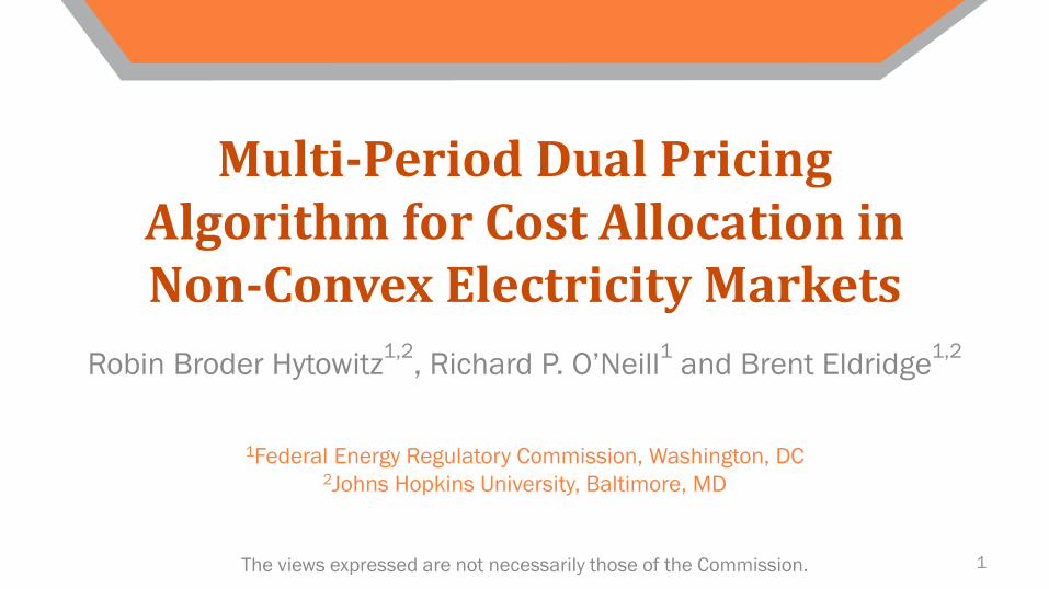
𝑑𝑑𝑖𝑖𝑡𝑡 Demand𝑝𝑝𝑖𝑖𝑡𝑡 Generator production variable 𝑢𝑢𝑖𝑖𝑡𝑡 Commitment variable (*=optimal)

𝑐𝑐𝑖𝑖𝑡𝑡, 𝑐𝑐𝑖𝑖𝑡𝑡𝑂𝑂𝑂𝑂 , 𝑐𝑐𝑖𝑖𝑆𝑆𝑆𝑆 Generator marginal and operating costs𝑝𝑝𝑖𝑖min, 𝑝𝑝𝑖𝑖max Generator min and max capacity

𝑏𝑏𝑖𝑖𝑡𝑡 Demand offer𝑑𝑑𝑖𝑖max Demand max capacity

max ∑𝑡𝑡∈𝑇𝑇 ∑𝑖𝑖∈𝐷𝐷 𝑏𝑏𝑖𝑖𝑡𝑡𝑑𝑑𝑖𝑖𝑡𝑡 − ∑𝑖𝑖∈𝐺𝐺 𝑐𝑐𝑖𝑖𝑡𝑡𝑝𝑝𝑖𝑖𝑡𝑡 + 𝑐𝑐𝑖𝑖𝑡𝑡𝑂𝑂𝑂𝑂𝑢𝑢𝑖𝑖𝑡𝑡 + 𝑐𝑐𝑖𝑖𝑆𝑆𝑆𝑆𝑧𝑧𝑖𝑖𝑡𝑡 Market surplus

∑𝑖𝑖∈𝐷𝐷 𝑑𝑑𝑖𝑖𝑡𝑡 − ∑𝑖𝑖∈𝐺𝐺 𝑝𝑝𝑖𝑖𝑡𝑡 = 0 ∀𝑡𝑡 ∈ 𝑇𝑇 Market clearing (𝜆𝜆𝑡𝑡)

𝑝𝑝𝑖𝑖min𝑢𝑢𝑖𝑖𝑡𝑡 ≤ 𝑝𝑝𝑖𝑖𝑡𝑡 ≤ 𝑝𝑝𝑖𝑖max𝑢𝑢𝑖𝑖𝑡𝑡 ∀𝑖𝑖 ∈ 𝐺𝐺,𝑡𝑡 ∈ 𝑇𝑇 Generation bounds

𝑢𝑢𝑖𝑖𝑡𝑡 − 𝑢𝑢𝑖𝑖,𝑡𝑡−1 ≤ 𝑧𝑧𝑖𝑖𝑡𝑡 ∀𝑖𝑖 ∈ 𝐺𝐺,𝑡𝑡 ∈ 𝑇𝑇 Commitment def.0 ≤ 𝑑𝑑𝑖𝑖 ≤ 𝑑𝑑𝑖𝑖max ∀𝑖𝑖 ∈ 𝐷𝐷,𝑡𝑡 ∈ 𝑇𝑇 Demand bounds

0 ≤ 𝑢𝑢𝑖𝑖𝑡𝑡 ≤ 1 ∀𝑖𝑖 ∈ 𝐺𝐺,𝑡𝑡 ∈ 𝑇𝑇 Relax commitment0 ≤ 𝑧𝑧𝑖𝑖𝑡𝑡 ≤ 1 ∀𝑖𝑖 ∈ 𝐺𝐺,𝑡𝑡 ∈ 𝑇𝑇 Relax startup

ELMP Pricing Model

11

𝑑𝑑𝑖𝑖𝑡𝑡 Demand𝑝𝑝𝑖𝑖𝑡𝑡 Generator production variable 𝑢𝑢𝑖𝑖𝑡𝑡 Commitment variable (*=optimal)

𝑐𝑐𝑖𝑖𝑡𝑡, 𝑐𝑐𝑖𝑖𝑡𝑡𝑂𝑂𝑂𝑂 , 𝑐𝑐𝑖𝑖𝑆𝑆𝑆𝑆 Generator marginal and operating costs𝑝𝑝𝑖𝑖min, 𝑝𝑝𝑖𝑖max Generator min and max capacity

𝑏𝑏𝑖𝑖𝑡𝑡 Demand offer𝑑𝑑𝑖𝑖max Demand max capacity

𝑑𝑑𝑖𝑖𝑡𝑡 Demand𝑝𝑝𝑖𝑖𝑡𝑡 Generator production variable 𝑢𝑢𝑖𝑖𝑡𝑡 Commitment variable (*=optimal)

𝑀𝑀𝑃𝑃/𝑁𝑁𝑃𝑃 Generators with a make whole payment / no payment

𝑐𝑐𝑖𝑖𝑡𝑡, 𝑐𝑐𝑖𝑖𝑡𝑡𝑂𝑂𝑂𝑂 , 𝑐𝑐𝑖𝑖𝑆𝑆𝑆𝑆 Generator marginal and operating costs𝑝𝑝𝑖𝑖min, 𝑝𝑝𝑖𝑖max Generator min and max capacity

𝑏𝑏𝑖𝑖𝑡𝑡 Demand offer𝑑𝑑𝑖𝑖max Demand max capacity

Average Incremental Cost Modelmax ∑𝑡𝑡∈𝑇𝑇 ∑𝑖𝑖∈𝐷𝐷 𝑏𝑏𝑖𝑖𝑡𝑡𝑑𝑑𝑖𝑖𝑡𝑡 − ∑𝑖𝑖∈𝐺𝐺𝑁𝑁𝑁𝑁 𝑐𝑐𝑖𝑖𝑡𝑡𝑝𝑝𝑖𝑖𝑡𝑡 − ∑𝑖𝑖∈𝐺𝐺𝑀𝑀𝑁𝑁 𝑐𝑐𝑖𝑖𝑡𝑡𝐴𝐴𝐴𝐴𝑂𝑂𝑝𝑝𝑖𝑖𝑡𝑡 Market surplus

∑𝑖𝑖∈𝐷𝐷 𝑑𝑑𝑖𝑖𝑡𝑡 − ∑𝑖𝑖∈𝐺𝐺 𝑝𝑝𝑖𝑖𝑡𝑡 = 0 ∀𝑡𝑡 ∈ 𝑇𝑇 Market clearing (𝜆𝜆𝑡𝑡)

0 ≤ 𝑝𝑝𝑖𝑖𝑡𝑡 ≤ 𝑝𝑝𝑖𝑖max𝑢𝑢𝑖𝑖𝑡𝑡∗ ∀𝑖𝑖 ∈ 𝐺𝐺𝑀𝑀𝑀𝑀,𝑡𝑡 ∈ 𝑇𝑇 Generation bounds

𝑝𝑝𝑖𝑖min𝑢𝑢𝑖𝑖𝑡𝑡∗ ≤ 𝑝𝑝𝑖𝑖𝑡𝑡 ≤ 𝑝𝑝𝑖𝑖max𝑢𝑢𝑖𝑖𝑡𝑡∗ ∀𝑖𝑖 ∈ 𝐺𝐺𝑁𝑁𝑀𝑀,𝑡𝑡 ∈ 𝑇𝑇 Generation bounds 0 ≤ 𝑑𝑑𝑖𝑖 ≤ 𝑑𝑑𝑖𝑖max ∀𝑖𝑖 ∈ 𝐷𝐷,𝑡𝑡 ∈ 𝑇𝑇 Demand bounds

12

𝑐𝑐𝑖𝑖𝑡𝑡𝐴𝐴𝐴𝐴𝑂𝑂 = 𝑐𝑐𝑖𝑖𝑡𝑡 +𝑐𝑐𝑖𝑖𝑡𝑡𝑂𝑂𝑂𝑂𝑢𝑢𝑖𝑖𝑡𝑡∗

𝑝𝑝𝑖𝑖𝑡𝑡∗+ �

𝑡𝑡∈𝑇𝑇

𝑐𝑐𝑖𝑖𝑆𝑆𝑆𝑆𝑢𝑢𝑖𝑖𝑡𝑡∗

𝑝𝑝𝑖𝑖𝑡𝑡∗

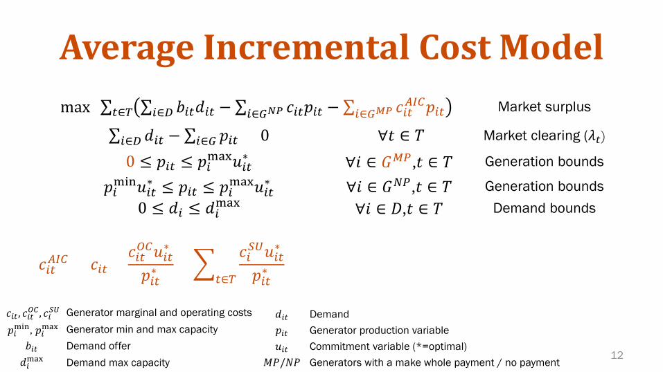
Comparative pricing methods

13

Name Description Price*

LMPLocational marginal price

Fix optimal solution, rerun to obtain prices c

ELMPExtended LMP

Relax binary commitment variable (MISO fast start pricing) c +

cOC

pmax

LIPLocational incremental price

Relax minimum to zero, use average incremental cost in objective c +

cOC

p∗

DPADual pricing algorithm

Proposed here λDPA

New Variables

• 𝜆𝜆DPA : new LMP

• 𝑢𝑢𝑖𝑖𝑝𝑝/𝑢𝑢𝑖𝑖

𝑝𝑝𝑑𝑑: make-whole payment

• 𝑢𝑢𝑖𝑖𝑐𝑐/𝑢𝑢𝑖𝑖𝑐𝑐𝑑𝑑 : make−whole charge

– Allocated by resource

14

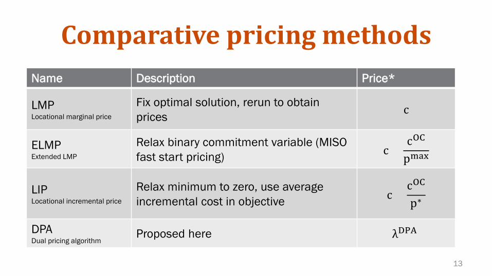
Multi-period formulation

15

min�𝑡𝑡∈𝑇𝑇

�𝑖𝑖∈𝐷𝐷+

𝑑𝑑𝑖𝑖𝑡𝑡∗ 𝑢𝑢𝑖𝑖𝑡𝑡𝑝𝑝𝑑𝑑 + �

𝑖𝑖∈𝐺𝐺+𝑝𝑝𝑖𝑖𝑡𝑡∗ 𝑢𝑢𝑖𝑖𝑡𝑡

𝑝𝑝 + 𝑐𝑐𝑢𝑢𝑝𝑝𝜆𝜆𝑡𝑡𝑢𝑢𝑝𝑝 + 𝑐𝑐𝑑𝑑𝑑𝑑𝜆𝜆𝑡𝑡𝑑𝑑𝑑𝑑 Uplift minimization

Subject to

�𝑡𝑡∈𝑇𝑇

�𝑖𝑖∈𝐷𝐷+

𝑑𝑑𝑖𝑖𝑡𝑡∗ 𝑢𝑢𝑖𝑖𝑡𝑡𝑝𝑝𝑑𝑑 − 𝑢𝑢𝑖𝑖𝑡𝑡𝑐𝑐𝑑𝑑 + �

𝑖𝑖∈𝐺𝐺+𝑝𝑝𝑖𝑖𝑡𝑡∗ 𝑢𝑢𝑖𝑖𝑡𝑡

𝑝𝑝 − 𝑢𝑢𝑖𝑖𝑡𝑡𝑐𝑐 = 0 Uplift revenue neutrality

Π𝑖𝑖 = �𝑡𝑡∈𝑇𝑇𝑟𝑟

𝑝𝑝𝑖𝑖𝑡𝑡∗ 𝜆𝜆𝑡𝑡𝐷𝐷𝑀𝑀𝐴𝐴 − 𝑐𝑐𝑖𝑖𝑡𝑡 + 𝑢𝑢𝑖𝑖𝑡𝑡𝑝𝑝 − 𝑢𝑢𝑖𝑖𝑡𝑡𝑐𝑐 − 𝑢𝑢𝑖𝑖𝑡𝑡∗ 𝑐𝑐𝑖𝑖𝑡𝑡𝑂𝑂𝑂𝑂 − 𝑧𝑧𝑖𝑖𝑡𝑡∗ 𝑐𝑐𝑖𝑖𝑆𝑆𝑆𝑆 ∀𝑖𝑖 ∈ 𝐺𝐺+ Profit definition

Ψ𝑖𝑖 = �𝑡𝑡∈𝑇𝑇𝑟𝑟

𝑑𝑑𝑖𝑖𝑡𝑡∗ 𝑏𝑏𝑖𝑖𝑡𝑡 − 𝜆𝜆𝑡𝑡𝐷𝐷𝑀𝑀𝐴𝐴 + 𝑢𝑢𝑖𝑖𝑡𝑡𝑝𝑝𝑑𝑑 − 𝑢𝑢𝑖𝑖𝑡𝑡𝑐𝑐𝑑𝑑 ∀𝑖𝑖 ∈ 𝐷𝐷+ Value definition

𝜆𝜆𝑡𝑡𝐷𝐷𝑀𝑀𝐴𝐴 − 𝜆𝜆𝑡𝑡∗ /𝜆𝜆𝑡𝑡∗ − 𝜆𝜆𝑡𝑡𝑢𝑢𝑝𝑝 + 𝜆𝜆𝑡𝑡𝑑𝑑𝑑𝑑 = 0 ∀𝑡𝑡 ∈ 𝑇𝑇 Price conditioning

𝜆𝜆𝑡𝑡𝐷𝐷𝑀𝑀𝐴𝐴 ≥ 𝑏𝑏𝑖𝑖𝑡𝑡 ∀𝑖𝑖 ∈ 𝐷𝐷0, 𝑡𝑡 ∈ 𝑇𝑇 Non-recourse conditionΨ𝑖𝑖 ≥ 0 ∀𝑖𝑖 ∈ 𝐷𝐷+ Non-confiscation of demand𝛱𝛱𝑖𝑖 ≥ 0 ∀𝑖𝑖 ∈ 𝐺𝐺+ Non-confiscation of supply

𝑢𝑢𝑖𝑖𝑡𝑡𝑝𝑝 ,𝑢𝑢𝑖𝑖𝑡𝑡𝑐𝑐 ,𝑢𝑢𝑖𝑖𝑡𝑡

𝑝𝑝𝑑𝑑 ,𝑢𝑢𝑖𝑖𝑡𝑡𝑐𝑐𝑑𝑑 ≥ 0 ∀𝑖𝑖 ∈ 𝐷𝐷⋃𝐺𝐺, 𝑡𝑡 ∈ 𝑇𝑇 Non-negativity

45

50

55

60

65

70

75

80

85

0 50 100 150 200 250 300

Pric

e ($

/MW

h)

Demand (MW)

LMP ELMP

16

Gen Min Cap(MW)

Max Cap (MW)

Marginal Cost($/MWh)

Operating cost($/h)

A 20 100 50 500

B 20 100 52 500

C 20 100 55 500

D 5 20 65 40

MISO example DPA reflects average incremental costs

• DPA and LIP prices are the same and have no uplift

• ELMP is increasing wrt demand

Example Source: Gribik, Zhang “Extended Locational marginal Pricing,” FERC Software Conference 2010

45

50

55

60

65

70

75

80

85

0 50 100 150 200 250 300

Pric

e ($

/MW

h)

Demand (MW)

LMP ELMP LIP DPA

-5

195

395

595

795

995

0 50 100 150 200 250 300U

plift

($)

Demand (MW)

Simple Multiperiod Example: Conditioning impacts prices across time

17

Hour 1 2 3 4 5 6 7 8 Uplift ($)

Dispatchedgenerator A A A A A A+B A+B A

LMP 𝜆𝜆𝑡𝑡∗

30 30 30 30 30 30 30 30 4500

𝜆𝜆𝑡𝑡𝐷𝐷𝑀𝑀𝐴𝐴 − 𝜆𝜆𝑡𝑡∗ /𝜆𝜆𝑡𝑡∗ − 𝜆𝜆𝑡𝑡𝑢𝑢𝑝𝑝 + 𝜆𝜆𝑡𝑡𝑑𝑑𝑑𝑑 = 0

𝜆𝜆𝑡𝑡𝐷𝐷𝑀𝑀𝐴𝐴 − 𝜆𝜆𝑡𝑡∗ /𝜆𝜆𝑡𝑡∗ − 𝜆𝜆𝑢𝑢𝑝𝑝 + 𝜆𝜆𝑑𝑑𝑑𝑑 = 0

Gen Min Cap(MW)

Max Cap (MW)

Marginal Cost($/MWh)

Operating cost($/h)

Startup cost ($/start)

A 200 1200 30 100 900

B 50 80 50 100 600

DPA, multi 𝜆𝜆𝑡𝑡DPA

30.22 30.22 30.22 30.22 30.22 30.22 30.22 30.22 Net 0*

DPA, single𝜆𝜆𝑡𝑡DPA′

30 30 30 30 30 86 30 30 0

*Demand pays Gen B $2779

Multiperiod Comparison:

18

Gen MinCap

(MW)

Max Cap

(MW)

Marginal Cost

($/MWh)

Operating cost($/h)

Startupcost

($/start)

A 200 1200 30 100 900

B 50 80 50 100 600

C 25 50 60 100 360

10

20

30

40

50

60

70

80

90

1 2 3 4 5 6 7 8

Pric

e($/

MW

h)

Time

LMP ELMP LIP

Dispatch A A A+B 𝐴𝐴+B 𝐴𝐴+B 𝐴𝐴+𝐵𝐵+𝐶𝐶 𝐴𝐴+𝐵𝐵+C A

Multiperiod Comparison: DPA prices follow LMP allocating uplift in peak period

• Uplift:– LMP $3110– ELMP $197– LIP $0– DPA $302

• Dem 2 pays $0.472/MWh to Gen C in period 7

19

Gen MinCap

(MW)

Max Cap

(MW)

Marginal Cost

($/MWh)

Operating cost($/h)

Startupcost

($/start)

A 200 1200 30 100 900

B 50 80 50 100 600

C 25 50 60 100 360

10

20

30

40

50

60

70

80

90

1 2 3 4 5 6 7 8

Pric

e($/

MW

h)

Time

LMP ELMP LIP DPA

Dispatch A A A+B 𝐴𝐴+B 𝐴𝐴+B 𝐴𝐴+𝐵𝐵+𝐶𝐶 𝐴𝐴+𝐵𝐵+C A𝜆𝜆𝑡𝑡𝐷𝐷𝑀𝑀𝐴𝐴 − 𝜆𝜆𝑡𝑡∗ /𝜆𝜆𝑡𝑡∗ − 𝜆𝜆𝑢𝑢𝑝𝑝 + 𝜆𝜆𝑑𝑑𝑑𝑑 = 0

Multiperiod Comparison:DPA prices slightly higher with no side payment

• Uplift:– LMP $3110– ELMP $197– LIP $0– DPA $0

20

Gen MinCap

(MW)

Max Cap

(MW)

Marginal Cost

($/MWh)

Operating cost($/h)

Startupcost

($/start)

A 200 1200 30 100 900

B 50 80 50 100 600

C 25 50 60 100 360

Dispatch A A A+B 𝐴𝐴+B 𝐴𝐴+B 𝐴𝐴+𝐵𝐵+𝐶𝐶 𝐴𝐴+𝐵𝐵+C A𝜆𝜆𝑡𝑡𝐷𝐷𝑀𝑀𝐴𝐴 − 𝜆𝜆𝑡𝑡∗ /𝜆𝜆𝑡𝑡∗ − 𝜆𝜆𝑡𝑡𝑢𝑢𝑝𝑝 + 𝜆𝜆𝑡𝑡𝑑𝑑𝑑𝑑 = 0

10

20

30

40

50

60

70

80

90

1 2 3 4 5 6 7 8

Pric

e ($

/MW

h)

Time

LMP ELMP LIP DPA

Properties of the DPA• Non-confiscation• Revenue neutral (and adequate)• Feasible solution with optimal feasible UC• Does not change optimal dispatch solution• Easy to implement in present ISO software• Problem is linear – computationally efficient • Price is non-unique

– Can be conditioned depending on operator preference 21

Thank you!

Questions?

robin.hytowitz@ferc.gov

22

What makes a good price?• In a non-convex market, the answer is not

straightforward – “Nomads in an intellectual desert” – Matt White – “An important objective of electricity market design is to

provide efficient prices with the associated incentives for operation and investment.” – Bill Hogan

• Incentives for operation: stay on dispatch• Incentives for investment: new resources entering the market

23

Comparison of methods: Trends in prices

• LIP • (DPA)

24LI

P ($

/MW

h)Quantity (MW)

supply

LMP

($/M

Wh)

Quantity (MW)

supply

• LMP (lighter)• ELMP

Example: Scarf• Modified Scarf example

25

0

1

2

3

4

5

6

7

8

3 23 43 63 83 103 123 143

Pric

e ($

/MW

h)

Demand (MW)

LMP UpliftOrig dLMP UpliftDPA

Historical Example: Canal Units• Canal Units on Cape Cod run daily due to long startup

times and regional specifications • Units support customers on Cape Cod

– Without that demand, they would not be needed• Uplift broadly allocated including Lower Southeastern

Massachusetts (SEMA)

Source: http://www.capecodtimes.com/article/20150716/NEWS/150719565

− SEMA does not benefit− Costs should have been allocated

primarily to Cape Cod to find a cheaper alternative much sooner

26

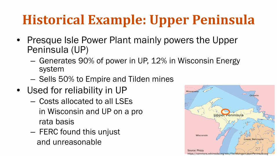
Historical Example: Upper Peninsula• Presque Isle Power Plant mainly powers the Upper

Peninsula (UP)– Generates 90% of power in UP, 12% in Wisconsin Energy

system– Sells 50% to Empire and Tilden mines

• Used for reliability in UP – Costs allocated to all LSEs

in Wisconsin and UP on a prorata basis

– FERC found this unjustand unreasonable

Source: Phizzyhttps://commons.wikimedia.org/wiki/File:MichiganUpperPeninsula.svg

27

Post-UC Pricing Model

i

i

i

zdp Cleared energy

Cleared demand Startup commitment 28

Decision variables

max ∑𝑖𝑖∈𝐷𝐷 𝑏𝑏𝑖𝑖𝑑𝑑𝑖𝑖 − ∑𝑖𝑖∈𝐺𝐺 𝑐𝑐𝑖𝑖𝑝𝑝𝑖𝑖 + 𝑐𝑐𝑖𝑖SU𝑧𝑧𝑖𝑖 Market surplus

∑𝑖𝑖∈𝐷𝐷 𝑑𝑑𝑖𝑖 − ∑𝑖𝑖∈𝐺𝐺 𝑝𝑝𝑖𝑖 = 0 𝜆𝜆 Market clearing

𝑝𝑝𝑖𝑖min𝑧𝑧𝑖𝑖 ≤ 𝑝𝑝𝑖𝑖 ≤ 𝑝𝑝𝑖𝑖max𝑧𝑧𝑖𝑖 ∀𝑖𝑖 ∈ 𝐺𝐺 𝛽𝛽𝑖𝑖max,𝛽𝛽𝑖𝑖min Generation bounds

0 ≤ 𝑑𝑑𝑖𝑖 ≤ 𝑑𝑑𝑖𝑖max ∀𝑖𝑖 ∈ 𝐷𝐷 𝛼𝛼𝑖𝑖max Demand bounds

𝑧𝑧𝑖𝑖 = 𝑧𝑧𝑖𝑖∗ ∀𝑖𝑖 ∈ 𝐺𝐺 𝛿𝛿𝑖𝑖 Fix optimal schedule

Dual Model

29

min ∑𝑖𝑖∈𝐷𝐷 𝑑𝑑𝑖𝑖max𝛼𝛼𝑖𝑖max + ∑𝑖𝑖∈𝐺𝐺 𝑧𝑧𝑖𝑖∗𝛿𝛿𝑖𝑖 Resource valuation

𝜆𝜆 + 𝛼𝛼𝑖𝑖max ≥ 𝑏𝑏𝑖𝑖 ∀𝑖𝑖 ∈ 𝐷𝐷 𝑑𝑑𝑖𝑖 Value condition

−𝜆𝜆 + 𝛽𝛽𝑖𝑖max − 𝛽𝛽𝑖𝑖min ≥ −𝑐𝑐𝑖𝑖 ∀𝑖𝑖 ∈ 𝐺𝐺 𝑝𝑝𝑖𝑖 Profit condition

𝛿𝛿𝑖𝑖 − 𝑝𝑝𝑖𝑖max𝛽𝛽𝑖𝑖max + 𝑝𝑝𝑖𝑖min𝛽𝛽𝑖𝑖min = −𝑐𝑐𝑖𝑖SU ∀𝑖𝑖 ∈ 𝐺𝐺 𝑧𝑧𝑖𝑖 Startup economics

𝛼𝛼𝑖𝑖max,𝛽𝛽𝑖𝑖max,𝛽𝛽𝑖𝑖min ≥ 0 ∀𝑖𝑖 ∈ 𝐷𝐷U𝐺𝐺 Non-negativity

Objective• Minimize uplift payments

• min∑𝑖𝑖∈𝐷𝐷+ 𝑑𝑑𝑖𝑖∗𝑢𝑢𝑖𝑖

pd + ∑𝑖𝑖∈𝐺𝐺+ 𝑝𝑝𝑖𝑖∗ 𝑢𝑢𝑖𝑖

p

• Uplift payments from demand and generation

30

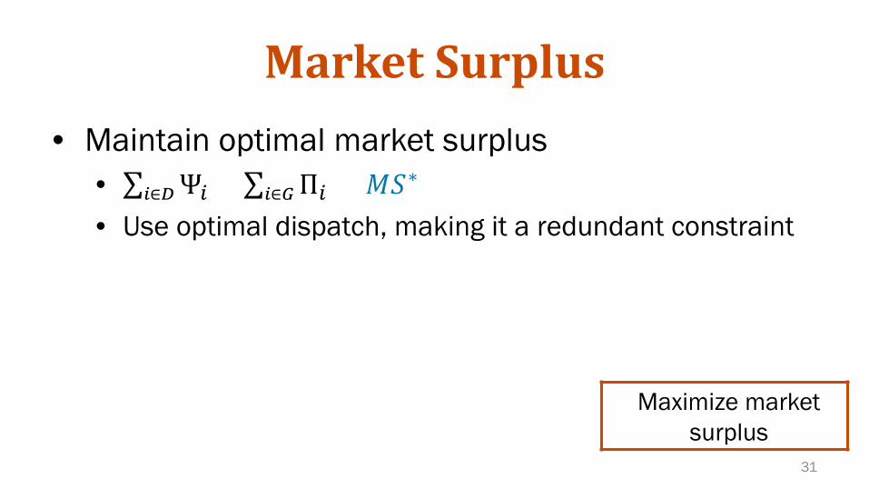
Market Surplus• Maintain optimal market surplus

• ∑𝑖𝑖∈𝐷𝐷Ψ𝑖𝑖 + ∑𝑖𝑖∈𝐺𝐺Π𝑖𝑖 = 𝑀𝑀𝑆𝑆∗

• Use optimal dispatch, making it a redundant constraint

31

Maximize market surplus

Profit Definition• From complementary slackness of the generation

bounds and the profit condition, combining with the startup economics, we calculate the linear surplus of generator i• 𝛿𝛿𝑖𝑖 = 𝑝𝑝𝑖𝑖∗ 𝜆𝜆 − 𝑐𝑐𝑖𝑖 − 𝑐𝑐𝑖𝑖𝑆𝑆𝑆𝑆

• dispatch*(LMP – marginal cost) – startup cost• To ensure non-confiscation, the linear surplus and

uplift payments must be non-negative• Π𝑖𝑖 = 𝛿𝛿𝑖𝑖 + 𝑝𝑝𝑖𝑖∗ 𝑢𝑢𝑖𝑖

𝑝𝑝 − 𝑢𝑢𝑖𝑖𝑐𝑐 ≥ 032

Non-confiscation

Value Definition• From complementary slackness of the value condition,

and non-negativity of variables, demand i• 𝑑𝑑𝑖𝑖∗ 𝑏𝑏𝑖𝑖 − 𝜆𝜆 = 𝑑𝑑𝑖𝑖∗𝛼𝛼𝑖𝑖𝑚𝑚𝑚𝑚𝑚𝑚∗ ≥ 0

• To ensure non-confiscation, the value and uplift payments must be non-negative• Ψ𝑖𝑖 = 𝑑𝑑𝑖𝑖∗𝛼𝛼𝑖𝑖𝑚𝑚𝑚𝑚𝑚𝑚∗ + 𝑑𝑑𝑖𝑖∗ 𝑢𝑢𝑖𝑖

𝑝𝑝 − 𝑢𝑢𝑖𝑖𝑐𝑐 ≥ 0

33

Non-confiscation

Additional constraints• Revenue neutrality

• ∑𝑖𝑖∈𝐷𝐷+ 𝑑𝑑𝑖𝑖∗ 𝑢𝑢𝑖𝑖

pd − 𝑢𝑢𝑖𝑖cd + ∑𝑖𝑖∈𝐺𝐺+ 𝑝𝑝𝑖𝑖∗ 𝑢𝑢𝑖𝑖

p − 𝑢𝑢𝑖𝑖c = 0

• Non-recourse of demand not selected• 𝜆𝜆DPA ≥ 𝑏𝑏𝑖𝑖• Value of new LMP not entice out-of-market demand to

consume

34

Revenue neutrality

Non-Unique Prices• Conditioning

• Allows the market operator to adjust LMP based on regional policies

• Example: tie new LMP to LMP from dispatch run

• New constraint: 𝜆𝜆DPA−𝜆𝜆∗

𝜆𝜆∗− 𝜆𝜆up + 𝜆𝜆dn = 0

• New Objective: min�

𝑖𝑖∈𝐷𝐷𝑑𝑑𝑖𝑖∗𝑢𝑢𝑖𝑖

pd + �𝑖𝑖∈𝐺𝐺𝑝𝑝𝑖𝑖∗ 𝑢𝑢𝑖𝑖

p + 𝑐𝑐up𝜆𝜆up + 𝑐𝑐dn𝜆𝜆dn

35

Example: Single node, single period

A B

100 $/MWh[0,100] MW

63 $/MWh[0,30] MW

40 $/MWh500 $/start

[0,40] MW

60 $/MWh500 $/start

[10,200] MW

1 236

Resulting UC Solution

A B

100 $/MWh100 MW

63 $/MWh30 MW

40 $/MWh500 $/start

40 MW

60 $/MWh500 $/start

90 MW

60 $/MWh

Market surplus = $3830

Gen Margin($/MWh)

Profit($)

A 20 300B 0 -500

Buyer Margin($/MWh)

NetValue

($)1 40 40002 3 90

1 2

Price = $60/MWh Uplift = $500

Avg. socialized uplift = $3.85/MWhPayment = 63.85 $/MWh 37

Results of DPA

Gen Marg. Cost up uc

A 40 0 0

B 60 0 0

Buyer Value up uc

1 100 0 0.767

2 63 2.556 0

λDPA Make whole paymentUnallocated make whole

payment

65.56 76.67 0

piu Make whole

paymentMake whole chargeNew LMPDPAλ

ciu

38

Results of DPA

Post-UC Value ($) Value under DPA ($)

LMP (λ) 60 65.56

Unit ($/MWh) Total Unit ($/MWh) Total

ProfitGen A 20 300 25.56

(+28%)522.22 (+74%)

Gen B 0 -500 5.56 0

Value Buyer 1 40 4000 33.678

(-19%)3367 (-19%)

Buyer 2 3 90 0 0

39

Comparison to Convex Hull• Convex hull formulation finds a uniform price that

minimizes side payments– Not all side payments minimized– Not well understood

• Formulation based on [1]

[1] D.A. Schiro, T. Zheng, F. Zhao, and E. Litvinov, “Convex Hull Pricing in Electricity Markets: Formulation, Analysis, and Implementation Challenges,” ISO-NE. [Online] Available: http://www.optimization-online.org/DB_FILE/2015/03/4830.pdf 40

Resulting CH Solution

A B

100 $/MWh100 MW

63 $/MWh30 MW

40 $/MWh500 $/start

40 MW

60 $/MWh500 $/start

90 MW

62.5 $/MWh

Market surplus = $4165

Gen Margin($/MWh)

Profit($)

A 20 400B 0 -275

Buyer Margin($/MWh)

NetValue

($)1 40 37502 3 15

1 2

Price = $62.50/MWh Uplift = $275

Avg. socialized uplift = $2.12/MWhPayment = 64.62 $/MWh 41

Results Comparison

Original Value Value under DPA Value under Convex Hull

LMP λ ($/MWh) 60 65.56 62.50

Unit ($/MWh) Total Unit

($/MWh) Total Unit ($/MWh) Total

Profit

Gen A($40/MWh)

20(-)

300(-)

25.56(+28%)

522.22 (+74%)

22.50(+13%)

400(+33%)

Gen B($60/MWh)

0 -500 5.56 0 2.50 -275

Value

Buyer 1($100/MWh)

40(-)

4000(-)

33.678(-19%)

3367 (-19%)

37.50(-6%)

3750(-6%)

Buyer 2($63/MWh)

3 90 0 0 0.50 15

42

Revenue Adequacy and LOCsMarket surplus = $200

GenMarginal Cost

($/MWh)Start Up

CostLinear Profit

($)Dispatch(MWh)

Max Capacity(MW)

Total Cost($)

A 30 900 1100 0 200 0B 40 100 -100 60 200 2500

LMP = $40/MWh Uplift = -$100 Avg. socialized uplift = -$1.67/MWh

BuyerValue

($/MWh)Load

(MWh)Max demand

(MW)

MarginalValue

($/MWh)

Total Value($)

Gross Value($)

1 45 60 60 5 300 2700

200 MWh($40/MWh-$30/MWh)-$900 = $1100 = LOC > MS = $20043