Embed Size (px)
Citation preview
Dual baseline search for muon antineutrino disappearance at 0.1 eV2 < ∆m2 < 100 eV21
G. Cheng,6, a W. Huelsnitz,15, b A. A. Aguilar-Arevalo,18 J. L. Alcaraz-Aunion,3 S. J. Brice,7 B. C. Brown,72
L. Bugel,17 J. Catala-Perez,24 E. D. Church,25 J. M. Conrad,17 R. Dharmapalan,1 Z. Djurcic,2 U. Dore,213
D. A. Finley,7 R. Ford,7 A. J. Franke,6 F. G. Garcia,7 G. T. Garvey,15 C. Giganti,21, c J. J. Gomez-Cadenas,244
J. Grange,8 P. Guzowski,10, d A. Hanson,11 Y. Hayato,12 K. Hiraide,14, e C. Ignarra,17 R. Imlay,16 R. A.5
Johnson,4 B. J. P. Jones,17 G. Jover-Manas,3 G. Karagiorgi,6, 17 T. Katori,11, 17 Y. K. Kobayashi,236
T. Kobilarcik,7 H. Kubo,14 Y. Kurimoto,14, f W. C. Louis,15 P. F. Loverre,21 L. Ludovici,21 K. B. M. Mahn,6, g7
C. Mariani,6, h W. Marsh,7 S. Masuike,23 K. Matsuoka,14 V. T. McGary,17 W. Metcalf,16 G. B. Mills,158
J. Mirabal,15 G. Mitsuka,13, i Y. Miyachi,23, j S. Mizugashira,23 C. D. Moore,7 J. Mousseau,8 Y. Nakajima,14, k9
T. Nakaya,14 R. Napora,20, l P. Nienaber,22 D. Orme,14 B. Osmanov,8 M. Otani,14 Z. Pavlovic,15 D. Perevalov,710
C. C. Polly,7 H. Ray,8 B. P. Roe,19 A. D. Russell,7 F. Sanchez,3 M. H. Shaevitz,6 T.-A. Shibata,2311
M. Sorel,24 J. Spitz,17 I. Stancu,1 R. J. Stefanski,7 H. Takei,23, m H.-K. Tanaka,17 M. Tanaka,9 R. Tayloe,1112
I. J. Taylor,10, n R. J. Tesarek,7 Y. Uchida,10 R. G. Van de Water,15 J. J. Walding,10, o M. O. Wascko,1013
D. H. White,15 H. B. White,7 D. A. Wickremasinghe,4 M. Yokoyama,14, p G. P. Zeller,7 and E. D. Zimmerman514
(MiniBooNE and SciBooNE Collaborations)15
1University of Alabama, Tuscaloosa, Alabama 35487, USA16
2Argonne National Laboratory, Argonne, Illinois 60439, USA17
3Institut de Fisica d’Altes Energies, Universitat Autonoma de Barcelona, E-08193 Bellaterra (Barcelona), Spain18
4University of Cincinnati, Cincinnati, Ohio 45221, USA19
5University of Colorado, Boulder, Colorado 80309, USA20
6Columbia University, New York, New York 10027, USA21
7Fermi National Accelerator Laboratory, Batavia, Illinois 60510, USA22
8University of Florida, Gainesville, Florida 32611, USA23
9High Energy Accelerator Research Organization (KEK), Tsukuba, Ibaraki 305-0801, Japan24
10Imperial College London, London SW7 2AZ, United Kingdom25
11Indiana University, Bloomington, Indiana 47405, USA26
12Kamioka Observatory, Institute for Cosmic Ray Research, University of Tokyo, Gifu 506-1205, Japan27
13Research Center for Cosmic Neutrinos, Institute for Cosmic Ray Research,28
University of Tokyo, Kashiwa, Chiba 277-8582, Japan29
14Kyoto University, Kyoto 606-8502, Japan30
15Los Alamos National Laboratory, Los Alamos, New Mexico 87545, USA31
16Louisiana State University, Baton Rouge, Louisiana 70803, USA32
17Massachusetts Institute of Technology, Cambridge, Massachusetts 02139, USA33
18Instituto de Ciencias Nucleares, Universidad Nacional Autonoma de Mexico, D.F. 04510, Mexico34
19University of Michigan, Ann Arbor, Michigan 48109, USA35
20Purdue University Calumet, Hammond, Indiana 46323, USA36
21Universita di Roma Sapienza, Dipartimento di Fisica and INFN, I-00185 Rome, Italy37
22Saint Mary’s University of Minnesota, Winona, Minnesota 55987, USA38
23Tokyo Institute of Technology, Tokyo 152-8551, Japan39
24Instituto de Fisica Corpuscular, Universidad de Valencia and CSIC, E-46071 Valencia, Spain40
25Yale University, New Haven, Connecticut 06520, USA41
(Dated: August 1, 2012)42
The MiniBooNE and SciBooNE collaborations report the results of a joint search for short base-43
line disappearance of νµ at Fermilab’s Booster Neutrino Beamline. The MiniBooNE Cherenkov44
detector and the SciBooNE tracking detector observe antineutrinos from the same beam, therefore45
the combined analysis of their datasets serves to partially constrain some of the flux and cross sec-46
tion uncertainties. Uncertainties in the νµ background were constrained by neutrino flux and cross47
section measurements performed in both detectors. A likelihood ratio method was used to set a48
90% confidence level upper limit on νµ disappearance that dramatically improves upon prior limits49
in the ∆m2=0.1–100 eV2 region.50
PACS numbers: 14.60.Lm, 14.60.Pq, 14.60.St51
a Corresponding author: [email protected] Corresponding author: [email protected] c Present address: DSM/Irfu/SPP, CEA Saclay, F-91191 Gif-sur-
2
I. INTRODUCTION1
Recently there has been increasing evidence for neu-2
trino oscillations in the ∆m2 ≈ 1 eV2 region. Such os-3
cillations could imply the existence of new sterile neu-4
trino species that do not participate in standard weak5
interactions but mix with the known neutrino flavors6
through additional mass eigenstates. The LSND [1] ex-7
periment observed an excess of νe-like events in a νµ8
beam. MiniBooNE [2–4] has observed an excess of νe-like9
and νe-like events, in a νµ beam and νµ beam, respec-10
tively. Additional evidence for short-baseline anomalies11
with L/E ≈ 1, where L is the neutrino path length in km12
and E the neutrino energy in GeV, includes the deficit of13
events observed in reactor antineutrino [5] and radioac-14
tive source neutrino [6] experiments. If these anomalies15
are due to neutrino oscillations in the ∆m2 ≈ 1 eV216
range, then sterile neutrinos may provide the additional17
mass eigenstate(s). Observation of νµ (νµ) disappearance18
in conjunction with νe (νe) appearance in this ∆m2 range19
would be a smoking-gun for the presence of these sterile20
neutrinos. Alternatively, constraining νµ (νµ) disappear-21
ance can, along with global νe (νe) disappearance data,22
constrain the oscillation interpretation of the νe (νe) ap-23
pearance signals in LSND and MiniBooNE [7].24
Searches for νµ and νµ disappearance in MiniBooNE25
were performed in 2009 [8]. No evidence for disappear-26
ance was found. The search for νµ disappearance was27
recently repeated in MiniBooNE with the inclusion of28
data from the SciBooNE detector in a joint analysis [9].29
Once again, the results were consistent with no νµ dis-30
appearance. The analysis presented here is an improved31
search for νµ disappearance using data from MiniBooNE32
Yvette, Franced Present address: The School of Physics and Astronomy, The Uni-versity of Manchester, Manchester, M13 9PL, United Kingdom
e Present address: Kamioka Observatory, Institute for Cosmic RayResearch, University of Tokyo, Gifu 506-1205, Japan
f Present address: Present address: High Energy Accelerator Re-search Organization (KEK), Tsukuba, Ibaraki 305-0801, Japan
g Present address: TRIUMF, Vancouver, British Columbia, V6T2A3, Canada
h Present address: Center for Neutrino Physics, Virginia Tech,Blacksburg, VA, USA
i Present address: Solar-Terrestrial Environment Laboratory,Nagoya University, Furo-cho, Chikusa-ku, Nagoya, Japan
j Present address: Yamagata University, Yamagata, 990-8560Japan
k Present address: Lawrence Berkeley National Laboratory, Berke-ley, CA 94720, USA
l Present address: Epic Systems, Inc.m Present address: Kitasato University, Tokyo, 108-8641 Japann Present address: Department of Physics and Astronomy, StateUniversity of New York, Stony Brook, New York 11794-3800,USA
o Present address: Department of Physics, Royal Holloway, Uni-versity of London, Egham, TW20 0EX, United Kingdom
p Present address: Department of Physics, University of Tokyo,Tokyo 113-0033, Japan
and SciBooNE taken while the Booster Neutrino Beam-33
line (BNB) operated in antineutrino mode.34
The Monte Carlo (MC) predictions for both Mini-35
BooNE and SciBooNE were updated to account for re-36
cent neutrino flux and cross section measurements made37
with both experiments. The data from both detectors38
were then simultaneously fit to a simple two-antineutrino39
oscillation model. Improved constraints on MC predic-40
tions, the inclusion of SciBooNE data, and a MiniBooNE41
antineutrino data set nearly three times larger than what42
was available for the original νµ disappearance analysis,43
have allowed a 90% confidence level upper limit to be set44
that dramatically improves upon prior limits in the ∆m245
= 0.1–100 eV2 region, pushing down into the region of46
parameter space of interest to sterile neutrino models.47
This paper is organized as follows. Section II describes48
the BNB and the MiniBooNE and SciBooNE detectors.49
Then, the simulation of neutrino interactions with nu-50
clei and subsequent detector responses are described in51
Section III. The event selection and reconstruction for52
both detectors are described in Section IV. The param-53
eters for the MC tuning and its systematic uncertainties54
are given in Section V. Section VI describes the analysis55
methodology. The results of the analysis are presented56
in Section VII, and the final conclusions are given in Sec-57
tion VIII.58
II. BEAMLINE AND EXPERIMENTAL59
APPARATUS60
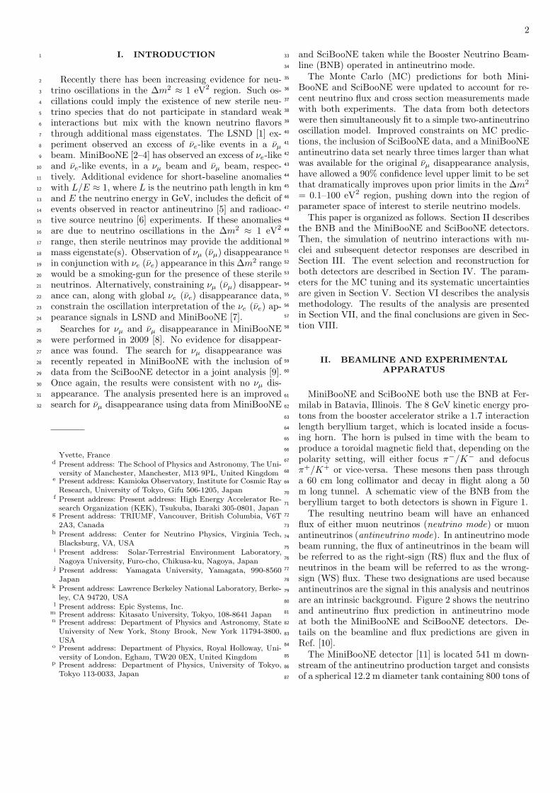
MiniBooNE and SciBooNE both use the BNB at Fer-61
milab in Batavia, Illinois. The 8 GeV kinetic energy pro-62
tons from the booster accelerator strike a 1.7 interaction63
length beryllium target, which is located inside a focus-64
ing horn. The horn is pulsed in time with the beam to65
produce a toroidal magnetic field that, depending on the66
polarity setting, will either focus π−/K− and defocus67
π+/K+ or vice-versa. These mesons then pass through68
a 60 cm long collimator and decay in flight along a 5069
m long tunnel. A schematic view of the BNB from the70
beryllium target to both detectors is shown in Figure 1.71
The resulting neutrino beam will have an enhanced72
flux of either muon neutrinos (neutrino mode) or muon73
antineutrinos (antineutrino mode). In antineutrino mode74
beam running, the flux of antineutrinos in the beam will75
be referred to as the right-sign (RS) flux and the flux of76
neutrinos in the beam will be referred to as the wrong-77
sign (WS) flux. These two designations are used because78
antineutrinos are the signal in this analysis and neutrinos79
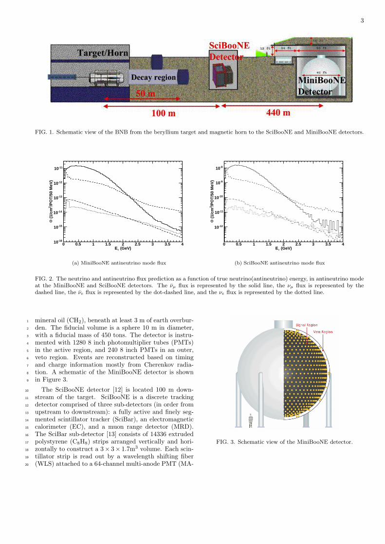
are an intrinsic background. Figure 2 shows the neutrino80
and antineutrino flux prediction in antineutrino mode81
at both the MiniBooNE and SciBooNE detectors. De-82
tails on the beamline and flux predictions are given in83
Ref. [10].84
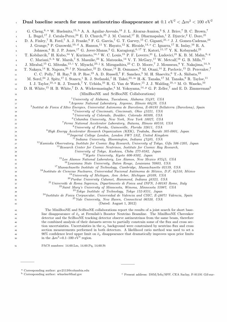
The MiniBooNE detector [11] is located 541 m down-85
stream of the antineutrino production target and consists86
of a spherical 12.2 m diameter tank containing 800 tons of87
3
FIG. 1. Schematic view of the BNB from the beryllium target and magnetic horn to the SciBooNE and MiniBooNE detectors.
(GeV)nE0 0.5 1 1.5 2 2.5 3 3.5 4
/PO
T/5
0 M
eV)
2 (
1/cm
F
-1610
-1510
-1410
-1310
-1210
-1110
(a) MiniBooNE antineutrino mode flux
(GeV)nE0 0.5 1 1.5 2 2.5 3 3.5 4
/PO
T/5
0 M
eV)
2 (
1/cm
F
-1210
-1110
-1010
-910
-810
(b) SciBooNE antineutrino mode flux
FIG. 2. The neutrino and antineutrino flux prediction as a function of true neutrino(antineutrino) energy, in antineutrino modeat the MiniBooNE and SciBooNE detectors. The νµ flux is represented by the solid line, the νµ flux is represented by thedashed line, the νe flux is represented by the dot-dashed line, and the νe flux is represented by the dotted line.
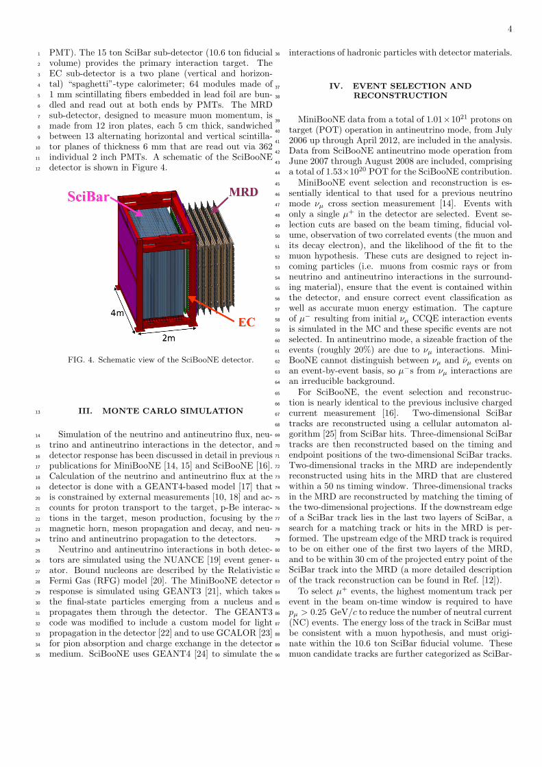
mineral oil (CH2), beneath at least 3 m of earth overbur-1
den. The fiducial volume is a sphere 10 m in diameter,2
with a fiducial mass of 450 tons. The detector is instru-3
mented with 1280 8 inch photomultiplier tubes (PMTs)4
in the active region, and 240 8 inch PMTs in an outer,5
veto region. Events are reconstructed based on timing6
and charge information mostly from Cherenkov radia-7
tion. A schematic of the MiniBooNE detector is shown8
in Figure 3.9
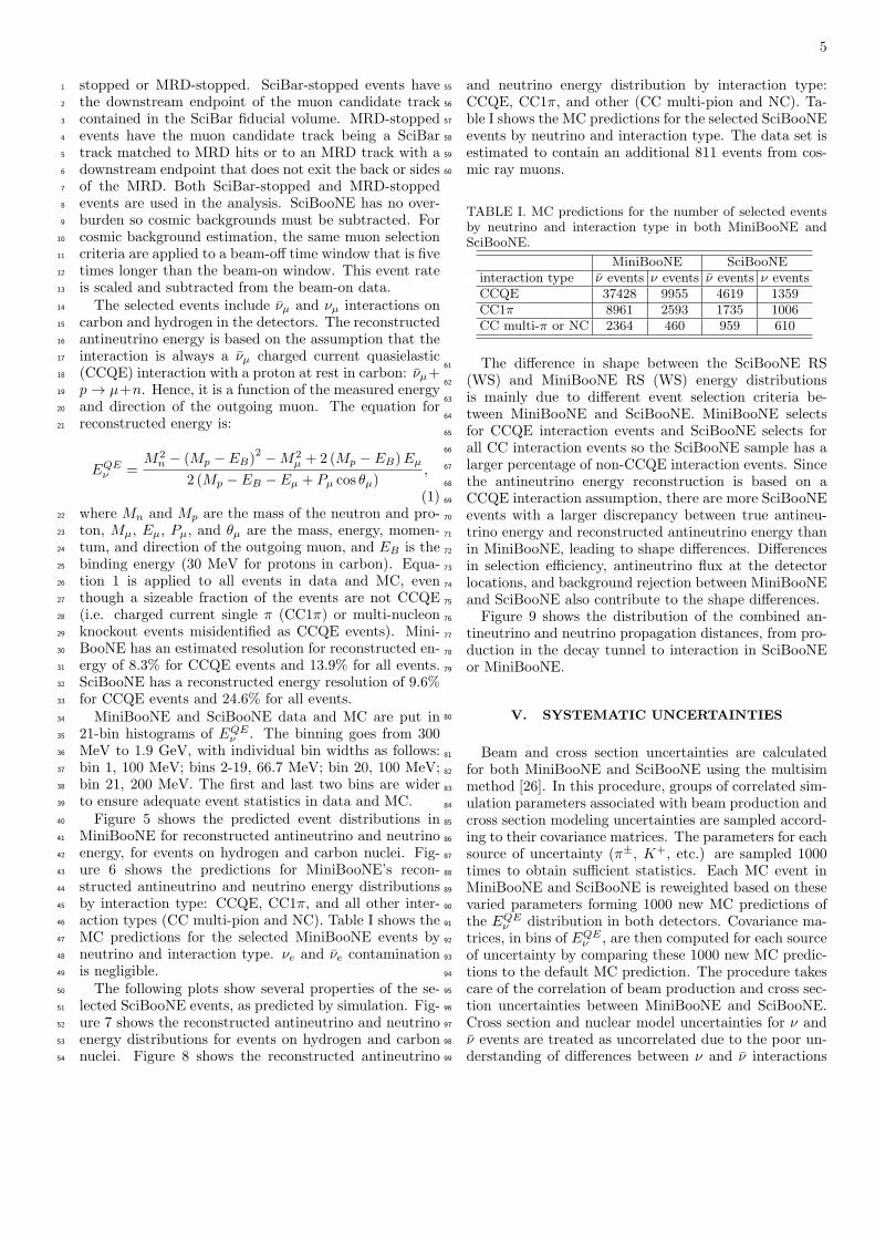
The SciBooNE detector [12] is located 100 m down-10
stream of the target. SciBooNE is a discrete tracking11
detector comprised of three sub-detectors (in order from12
upstream to downstream): a fully active and finely seg-13
mented scintillator tracker (SciBar), an electromagnetic14
calorimeter (EC), and a muon range detector (MRD).15
The SciBar sub-detector [13] consists of 14336 extruded16
polystyrene (C8H8) strips arranged vertically and hori-17
zontally to construct a 3× 3× 1.7m3 volume. Each scin-18
tillator strip is read out by a wavelength shifting fiber19
(WLS) attached to a 64-channel multi-anode PMT (MA-20
FIG. 3. Schematic view of the MiniBooNE detector.
4
PMT). The 15 ton SciBar sub-detector (10.6 ton fiducial1
volume) provides the primary interaction target. The2
EC sub-detector is a two plane (vertical and horizon-3
tal) “spaghetti”-type calorimeter; 64 modules made of4
1 mm scintillating fibers embedded in lead foil are bun-5
dled and read out at both ends by PMTs. The MRD6
sub-detector, designed to measure muon momentum, is7
made from 12 iron plates, each 5 cm thick, sandwiched8
between 13 alternating horizontal and vertical scintilla-9
tor planes of thickness 6 mm that are read out via 36210
individual 2 inch PMTs. A schematic of the SciBooNE11
detector is shown in Figure 4.12
FIG. 4. Schematic view of the SciBooNE detector.
III. MONTE CARLO SIMULATION13
Simulation of the neutrino and antineutrino flux, neu-14
trino and antineutrino interactions in the detector, and15
detector response has been discussed in detail in previous16
publications for MiniBooNE [14, 15] and SciBooNE [16].17
Calculation of the neutrino and antineutrino flux at the18
detector is done with a GEANT4-based model [17] that19
is constrained by external measurements [10, 18] and ac-20
counts for proton transport to the target, p-Be interac-21
tions in the target, meson production, focusing by the22
magnetic horn, meson propagation and decay, and neu-23
trino and antineutrino propagation to the detectors.24
Neutrino and antineutrino interactions in both detec-25
tors are simulated using the NUANCE [19] event gener-26
ator. Bound nucleons are described by the Relativistic27
Fermi Gas (RFG) model [20]. The MiniBooNE detector28
response is simulated using GEANT3 [21], which takes29
the final-state particles emerging from a nucleus and30
propagates them through the detector. The GEANT331
code was modified to include a custom model for light32
propagation in the detector [22] and to use GCALOR [23]33
for pion absorption and charge exchange in the detector34
medium. SciBooNE uses GEANT4 [24] to simulate the35
interactions of hadronic particles with detector materials.36
IV. EVENT SELECTION AND37
RECONSTRUCTION38
MiniBooNE data from a total of 1.01×10²¹ protons on39
target (POT) operation in antineutrino mode, from July40
2006 up through April 2012, are included in the analysis.41
Data from SciBooNE antineutrino mode operation from42
June 2007 through August 2008 are included, comprising43
a total of 1.53×10²⁰ POT for the SciBooNE contribution.44
MiniBooNE event selection and reconstruction is es-45
sentially identical to that used for a previous neutrino46
mode νµ cross section measurement [14]. Events with47
only a single µ+ in the detector are selected. Event se-48
lection cuts are based on the beam timing, fiducial vol-49
ume, observation of two correlated events (the muon and50
its decay electron), and the likelihood of the fit to the51
muon hypothesis. These cuts are designed to reject in-52
coming particles (i.e. muons from cosmic rays or from53
neutrino and antineutrino interactions in the surround-54
ing material), ensure that the event is contained within55
the detector, and ensure correct event classification as56
well as accurate muon energy estimation. The capture57
of µ− resulting from initial νµ CCQE interaction events58
is simulated in the MC and these specific events are not59
selected. In antineutrino mode, a sizeable fraction of the60
events (roughly 20%) are due to νµ interactions. Mini-61
BooNE cannot distinguish between νµ and νµ events on62
an event-by-event basis, so µ−s from νµ interactions are63
an irreducible background.64
For SciBooNE, the event selection and reconstruc-65
tion is nearly identical to the previous inclusive charged66
current measurement [16]. Two-dimensional SciBar67
tracks are reconstructed using a cellular automaton al-68
gorithm [25] from SciBar hits. Three-dimensional SciBar69
tracks are then reconstructed based on the timing and70
endpoint positions of the two-dimensional SciBar tracks.71
Two-dimensional tracks in the MRD are independently72
reconstructed using hits in the MRD that are clustered73
within a 50 ns timing window. Three-dimensional tracks74
in the MRD are reconstructed by matching the timing of75
the two-dimensional projections. If the downstream edge76
of a SciBar track lies in the last two layers of SciBar, a77
search for a matching track or hits in the MRD is per-78
formed. The upstream edge of the MRD track is required79
to be on either one of the first two layers of the MRD,80
and to be within 30 cm of the projected entry point of the81
SciBar track into the MRD (a more detailed description82
of the track reconstruction can be found in Ref. [12]).83
To select µ+ events, the highest momentum track per84
event in the beam on-time window is required to have85
pµ > 0.25 GeV/c to reduce the number of neutral current86
(NC) events. The energy loss of the track in SciBar must87
be consistent with a muon hypothesis, and must origi-88
nate within the 10.6 ton SciBar fiducial volume. These89
muon candidate tracks are further categorized as SciBar-90
5
stopped or MRD-stopped. SciBar-stopped events have1
the downstream endpoint of the muon candidate track2
contained in the SciBar fiducial volume. MRD-stopped3
events have the muon candidate track being a SciBar4
track matched to MRD hits or to an MRD track with a5
downstream endpoint that does not exit the back or sides6
of the MRD. Both SciBar-stopped and MRD-stopped7
events are used in the analysis. SciBooNE has no over-8
burden so cosmic backgrounds must be subtracted. For9
cosmic background estimation, the same muon selection10
criteria are applied to a beam-off time window that is five11
times longer than the beam-on window. This event rate12
is scaled and subtracted from the beam-on data.13
The selected events include νµ and νµ interactions on14
carbon and hydrogen in the detectors. The reconstructed15
antineutrino energy is based on the assumption that the16
interaction is always a νµ charged current quasielastic17
(CCQE) interaction with a proton at rest in carbon: νµ+18
p → µ+n. Hence, it is a function of the measured energy19
and direction of the outgoing muon. The equation for20
reconstructed energy is:21
EQEν =
M2n − (Mp − EB)
2 −M2µ + 2 (Mp − EB)Eµ
2 (Mp − EB − Eµ + Pµ cos θµ),
(1)where Mn and Mp are the mass of the neutron and pro-22
ton, Mµ, Eµ, Pµ, and θµ are the mass, energy, momen-23
tum, and direction of the outgoing muon, and EB is the24
binding energy (30 MeV for protons in carbon). Equa-25
tion 1 is applied to all events in data and MC, even26
though a sizeable fraction of the events are not CCQE27
(i.e. charged current single π (CC1π) or multi-nucleon28
knockout events misidentified as CCQE events). Mini-29
BooNE has an estimated resolution for reconstructed en-30
ergy of 8.3% for CCQE events and 13.9% for all events.31
SciBooNE has a reconstructed energy resolution of 9.6%32
for CCQE events and 24.6% for all events.33
MiniBooNE and SciBooNE data and MC are put in34
21-bin histograms of EQEν . The binning goes from 30035
MeV to 1.9 GeV, with individual bin widths as follows:36
bin 1, 100 MeV; bins 2-19, 66.7 MeV; bin 20, 100 MeV;37
bin 21, 200 MeV. The first and last two bins are wider38
to ensure adequate event statistics in data and MC.39
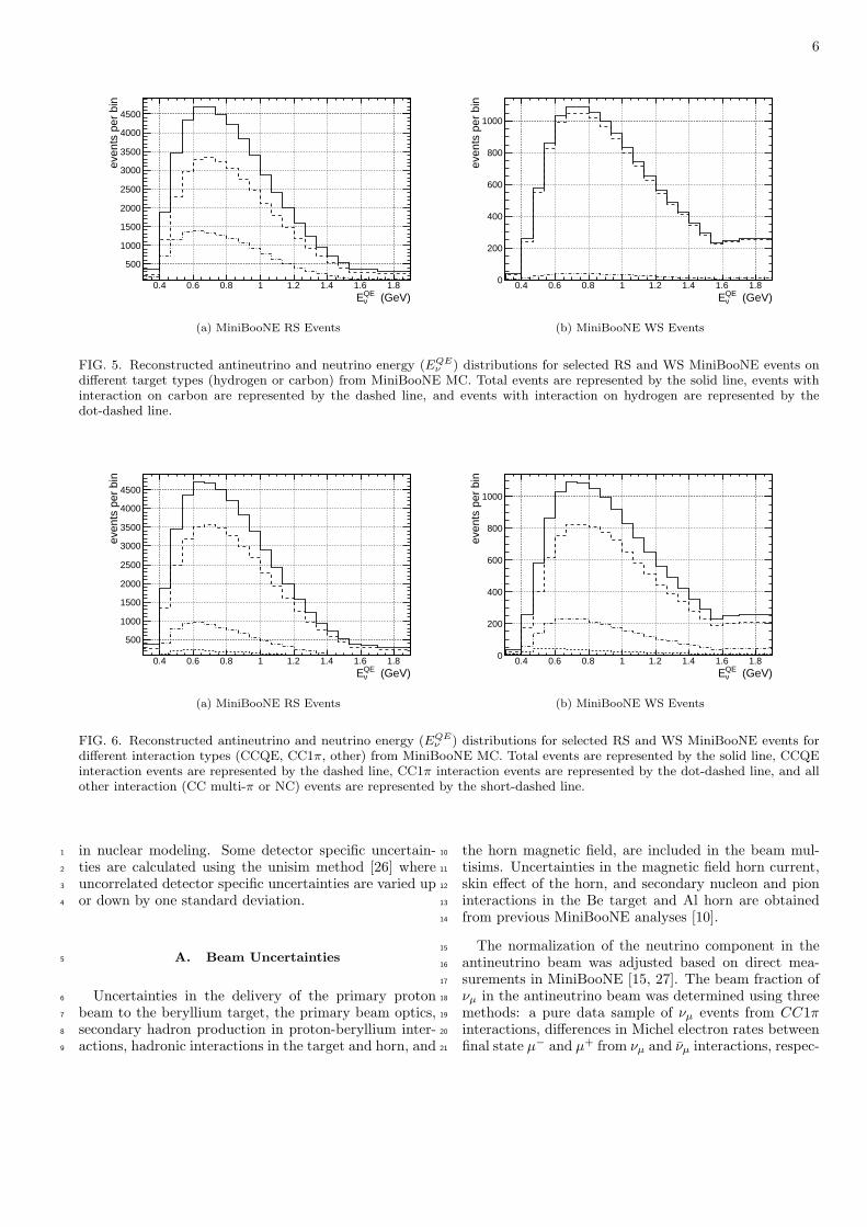
Figure 5 shows the predicted event distributions in40
MiniBooNE for reconstructed antineutrino and neutrino41
energy, for events on hydrogen and carbon nuclei. Fig-42
ure 6 shows the predictions for MiniBooNE’s recon-43
structed antineutrino and neutrino energy distributions44
by interaction type: CCQE, CC1π, and all other inter-45
action types (CC multi-pion and NC). Table I shows the46
MC predictions for the selected MiniBooNE events by47
neutrino and interaction type. νe and νe contamination48
is negligible.49
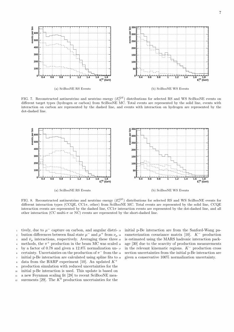
The following plots show several properties of the se-50
lected SciBooNE events, as predicted by simulation. Fig-51
ure 7 shows the reconstructed antineutrino and neutrino52
energy distributions for events on hydrogen and carbon53
nuclei. Figure 8 shows the reconstructed antineutrino54
and neutrino energy distribution by interaction type:55
CCQE, CC1π, and other (CC multi-pion and NC). Ta-56
ble I shows the MC predictions for the selected SciBooNE57
events by neutrino and interaction type. The data set is58
estimated to contain an additional 811 events from cos-59
mic ray muons.60
TABLE I. MC predictions for the number of selected eventsby neutrino and interaction type in both MiniBooNE andSciBooNE.
MiniBooNE SciBooNEinteraction type ν events ν events ν events ν eventsCCQE 37428 9955 4619 1359CC1π 8961 2593 1735 1006CC multi-π or NC 2364 460 959 610
The difference in shape between the SciBooNE RS61
(WS) and MiniBooNE RS (WS) energy distributions62
is mainly due to different event selection criteria be-63
tween MiniBooNE and SciBooNE. MiniBooNE selects64
for CCQE interaction events and SciBooNE selects for65
all CC interaction events so the SciBooNE sample has a66
larger percentage of non-CCQE interaction events. Since67
the antineutrino energy reconstruction is based on a68
CCQE interaction assumption, there are more SciBooNE69
events with a larger discrepancy between true antineu-70
trino energy and reconstructed antineutrino energy than71
in MiniBooNE, leading to shape differences. Differences72
in selection efficiency, antineutrino flux at the detector73
locations, and background rejection between MiniBooNE74
and SciBooNE also contribute to the shape differences.75
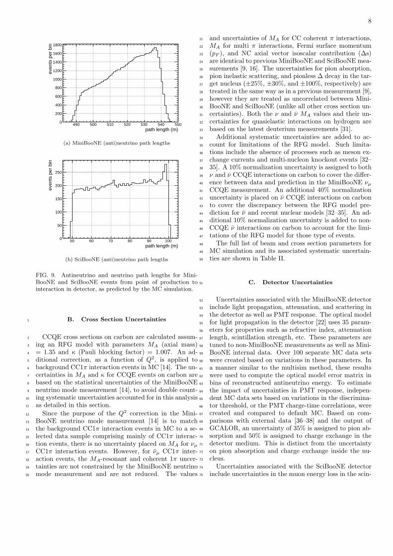
Figure 9 shows the distribution of the combined an-76
tineutrino and neutrino propagation distances, from pro-77
duction in the decay tunnel to interaction in SciBooNE78
or MiniBooNE.79
V. SYSTEMATIC UNCERTAINTIES80
Beam and cross section uncertainties are calculated81
for both MiniBooNE and SciBooNE using the multisim82
method [26]. In this procedure, groups of correlated sim-83
ulation parameters associated with beam production and84
cross section modeling uncertainties are sampled accord-85
ing to their covariance matrices. The parameters for each86
source of uncertainty (π±, K+, etc.) are sampled 100087
times to obtain sufficient statistics. Each MC event in88
MiniBooNE and SciBooNE is reweighted based on these89
varied parameters forming 1000 new MC predictions of90
the EQEν distribution in both detectors. Covariance ma-91
trices, in bins of EQEν , are then computed for each source92
of uncertainty by comparing these 1000 new MC predic-93
tions to the default MC prediction. The procedure takes94
care of the correlation of beam production and cross sec-95
tion uncertainties between MiniBooNE and SciBooNE.96
Cross section and nuclear model uncertainties for ν and97
ν events are treated as uncorrelated due to the poor un-98
derstanding of differences between ν and ν interactions99
6
(GeV)QEnE
0.4 0.6 0.8 1 1.2 1.4 1.6 1.8
even
ts p
er b
in
500
1000
1500
2000
2500
3000
3500
4000
4500
(a) MiniBooNE RS Events
(GeV)QEnE
0.4 0.6 0.8 1 1.2 1.4 1.6 1.8
even
ts p
er b
in
0
200
400
600
800
1000
(b) MiniBooNE WS Events
FIG. 5. Reconstructed antineutrino and neutrino energy (EQEν ) distributions for selected RS and WS MiniBooNE events on
different target types (hydrogen or carbon) from MiniBooNE MC. Total events are represented by the solid line, events withinteraction on carbon are represented by the dashed line, and events with interaction on hydrogen are represented by thedot-dashed line.
(GeV)QEnE
0.4 0.6 0.8 1 1.2 1.4 1.6 1.8
even
ts p
er b
in
500
1000
1500
2000
2500
3000
3500
4000
4500
(a) MiniBooNE RS Events
(GeV)QEnE
0.4 0.6 0.8 1 1.2 1.4 1.6 1.8
even
ts p
er b
in
0
200
400
600
800
1000
(b) MiniBooNE WS Events
FIG. 6. Reconstructed antineutrino and neutrino energy (EQEν ) distributions for selected RS and WS MiniBooNE events for
different interaction types (CCQE, CC1π, other) from MiniBooNE MC. Total events are represented by the solid line, CCQEinteraction events are represented by the dashed line, CC1π interaction events are represented by the dot-dashed line, and allother interaction (CC multi-π or NC) events are represented by the short-dashed line.
in nuclear modeling. Some detector specific uncertain-1
ties are calculated using the unisim method [26] where2
uncorrelated detector specific uncertainties are varied up3
or down by one standard deviation.4
A. Beam Uncertainties5
Uncertainties in the delivery of the primary proton6
beam to the beryllium target, the primary beam optics,7
secondary hadron production in proton-beryllium inter-8
actions, hadronic interactions in the target and horn, and9
the horn magnetic field, are included in the beam mul-10
tisims. Uncertainties in the magnetic field horn current,11
skin effect of the horn, and secondary nucleon and pion12
interactions in the Be target and Al horn are obtained13
from previous MiniBooNE analyses [10].14
The normalization of the neutrino component in the15
antineutrino beam was adjusted based on direct mea-16
surements in MiniBooNE [15, 27]. The beam fraction of17
νµ in the antineutrino beam was determined using three18
methods: a pure data sample of νµ events from CC1π19
interactions, differences in Michel electron rates between20
final state µ− and µ+ from νµ and νµ interactions, respec-21
7
(GeV)QEnE
0.4 0.6 0.8 1 1.2 1.4 1.6 1.8
even
ts p
er b
in
0
100
200
300
400
500
600
(a) SciBooNE RS Events
(GeV)QEnE
0.4 0.6 0.8 1 1.2 1.4 1.6 1.8
even
ts p
er b
in
0
50
100
150
200
250
300
350
(b) SciBooNE WS Events
FIG. 7. Reconstructed antineutrino and neutrino energy (EQEν ) distributions for selected RS and WS SciBooNE events on
different target types (hydrogen or carbon) from SciBooNE MC. Total events are represented by the solid line, events withinteraction on carbon are represented by the dashed line, and events with interaction on hydrogen are represented by thedot-dashed line.
(GeV)QEnE
0.4 0.6 0.8 1 1.2 1.4 1.6 1.8
even
ts p
er b
in
0
100
200
300
400
500
600
(a) SciBooNE RS Events
(GeV)QEnE
0.4 0.6 0.8 1 1.2 1.4 1.6 1.8
even
ts p
er b
in
0
50
100
150
200
250
300
350
(b) SciBooNE WS Events
FIG. 8. Reconstructed antineutrino and neutrino energy (EQEν ) distributions for selected RS and WS SciBooNE events for
different interaction types (CCQE, CC1π, other) from SciBooNE MC. Total events are represented by the solid line, CCQEinteraction events are represented by the dashed line, CC1π interaction events are represented by the dot-dashed line, and allother interaction (CC multi-π or NC) events are represented by the short-dashed line.
tively, due to µ− capture on carbon, and angular distri-1
bution differences between final state µ− and µ+ from νµ2
and νµ interactions, respectively. Averaging these three3
methods, the π+ production in the beam MC was scaled4
by a factor of 0.78 and given a 12.8% normalization un-5
certainty. Uncertainties on the production of π− from the6
initial p-Be interaction are calculated using spline fits to7
data from the HARP experiment [10]. An updated K+8
production simulation with reduced uncertainties for the9
initial p-Be interaction is used. This update is based on10
a new Feynman scaling fit [28] to recent SciBooNE mea-11
surements [29]. The K0 production uncertainties for the12
initial p-Be interaction are from the Sanford-Wang pa-13
rameterization covariance matrix [10]. K− production14
is estimated using the MARS hadronic interaction pack-15
age [30] due to the scarcity of production measurements16
in the relevant kinematic regions. K− production cross17
section uncertainties from the initial p-Be interaction are18
given a conservative 100% normalization uncertainty.19
8
path length (m)490 500 510 520 530 540 550
even
ts p
er b
in
0
200
400
600
800
1000
1200
1400
1600
1800
(a) MiniBooNE (anti)neutrino path lengths
path length (m)50 60 70 80 90 100
even
ts p
er b
in
0
50
100
150
200
250
(b) SciBooNE (anti)neutrino path lengths
FIG. 9. Antineutrino and neutrino path lengths for Mini-BooNE and SciBooNE events from point of production tointeraction in detector, as predicted by the MC simulation.
B. Cross Section Uncertainties1
CCQE cross sections on carbon are calculated assum-2
ing an RFG model with parameters MA (axial mass)3
= 1.35 and κ (Pauli blocking factor) = 1.007. An ad-4
ditional correction, as a function of Q2, is applied to5
background CC1π interaction events in MC [14]. The un-6
certainties in MA and κ for CCQE events on carbon are7
based on the statistical uncertainties of the MiniBooNE8
neutrino mode measurement [14], to avoid double count-9
ing systematic uncertainties accounted for in this analysis10
as detailed in this section.11
Since the purpose of the Q2 correction in the Mini-12
BooNE neutrino mode measurement [14] is to match13
the background CC1π interaction events in MC to a se-14
lected data sample comprising mainly of CC1π interac-15
tion events, there is no uncertainty placed on MA for νµ16
CC1π interaction events. However, for νµ CC1π inter-17
action events, the MA-resonant and coherent 1π uncer-18
tainties are not constrained by the MiniBooNE neutrino19
mode measurement and are not reduced. The values20
and uncertainties of MA for CC coherent π interactions,21
MA for multi π interactions, Fermi surface momentum22
(pF ), and NC axial vector isoscalar contribution (∆s)23
are identical to previous MiniBooNE and SciBooNE mea-24
surements [9, 16]. The uncertainties for pion absorption,25
pion inelastic scattering, and pionless ∆ decay in the tar-26
get nucleus (±25%, ±30%, and ±100%, respectively) are27
treated in the same way as in a previous measurement [9],28
however they are treated as uncorrelated between Mini-29
BooNE and SciBooNE (unlike all other cross section un-30
certainties). Both the ν and ν MA values and their un-31
certainties for quasielastic interactions on hydrogen are32
based on the latest deuterium measurements [31].33
Additional systematic uncertainties are added to ac-34
count for limitations of the RFG model. Such limita-35
tions include the absence of processes such as meson ex-36
change currents and multi-nucleon knockout events [32–37
35]. A 10% normalization uncertainty is assigned to both38
ν and ν CCQE interactions on carbon to cover the differ-39
ence between data and prediction in the MiniBooNE νµ40
CCQE measurement. An additional 40% normalization41
uncertainty is placed on ν CCQE interactions on carbon42
to cover the discrepancy between the RFG model pre-43
diction for ν and recent nuclear models [32–35]. An ad-44
ditional 10% normalization uncertainty is added to non-45
CCQE ν interactions on carbon to account for the limi-46
tations of the RFG model for those type of events.47
The full list of beam and cross section parameters for48
MC simulation and its associated systematic uncertain-49
ties are shown in Table II.50
C. Detector Uncertainties51
Uncertainties associated with the MiniBooNE detector52
include light propagation, attenuation, and scattering in53
the detector as well as PMT response. The optical model54
for light propagation in the detector [22] uses 35 param-55
eters for properties such as refractive index, attenuation56
length, scintillation strength, etc. These parameters are57
tuned to non-MiniBooNE measurements as well as Mini-58
BooNE internal data. Over 100 separate MC data sets59
were created based on variations in these parameters. In60
a manner similar to the multisim method, these results61
were used to compute the optical model error matrix in62
bins of reconstructed antineutrino energy. To estimate63
the impact of uncertainties in PMT response, indepen-64
dent MC data sets based on variations in the discrimina-65
tor threshold, or the PMT charge-time correlations, were66
created and compared to default MC. Based on com-67
parisons with external data [36–38] and the output of68
GCALOR, an uncertainty of 35% is assigned to pion ab-69
sorption and 50% is assigned to charge exchange in the70
detector medium. This is distinct from the uncertainty71
on pion absorption and charge exchange inside the nu-72
cleus.73
Uncertainties associated with the SciBooNE detector74
include uncertainties in the muon energy loss in the scin-75
9
tillator and iron, light attenuation in the wavelength1
shifting fibers, and PMT response; see Ref. [16]. The2
crosstalk of the MA-PMT was measured to be 3.15% for3
adjacent channels with an absolute error of 0.4% [12].4
The single photoelectron resolution of the MA-PMT is5
set to 50% in the simulation, and the absolute error is6
estimated to be ±20%. Birk’s constant for quenching in7
the SciBar scintillator was measured to be 0.0208±0.00238
cm/MeV [12]. The conversion factors for ADC counts to9
photoelectrons were measured for all 14,336 MA-PMT10
channels in SciBar. The measurement uncertainty was at11
the 20% level. The threshold for hits to be used in SciBar12
track reconstruction is 2.5 photoelectrons; this threshold13
is varied by ±20% to evaluate the systematic error for14
SciBar track reconstruction. The TDC dead time is set15
to 55 ns in the MC simulation, with the error estimated16
to be ±20 ns [39].17
The reconstruction uncertainties consist of antineu-18
trino energy reconstruction uncertainties and muon track19
misidentification uncertainties. For antineutrino energy20
reconstruction uncertainties, the densities of SciBar, EC,21
and MRD are varied independently within their mea-22
sured uncertainties of ±3%, ±10%, and ±3%, respec-23
tively. Misidentified muons stem mainly from proton24
tracks created through NC interactions, which are given25
a conservative ±20% normalization uncertainty. A con-26
servative ±20% normalization uncertainty is applied for27
the MC simulated background of neutrino and antineu-28
trino events initially interacting outside the SciBooNE29
detector that pass the selection criteria. A conserva-30
tive ±20% normalization uncertainty is applied for the31
MC simulated background of neutrino and antineutrino32
events initially interacting in the EC/MRD detector that33
pass the selection criteria.34
D. Error Matrix35
All of the MiniBooNE uncertainties, the SciBooNE un-36
certainties, and the correlations between them are ex-37
pressed in the total error matrix, M , a 42 × 42 covari-38
ance matrix in MiniBooNE and SciBooNE reconstructed39
antineutrino energy bins defined as:40
M =
(MMB-SB MSB-SB
MMB-MB MSB-MB
)(2)
where41
MXi,j = MX
i,j;(RS,RS)NY RSi NZ RS
j
+ MXi,j;(WS,WS)N
Y WSi NZ WS
j
+ MXi,j;(RS,WS)N
Y RSi NZ WS
j
+ MXi,j;(WS,RS)N
Y WSi NZ RS
j
+MX stati,j (3)
are the bin to bin covariance elements of the full error ma-42
trix. X denotes the type of correlation with Y and Z de-43
noting the type of bins (either MiniBooNE or SciBooNE)44
associated with X. For MiniBooNE to MiniBooNE cor-45
relations, X=MB-MB, Y=MB, Z=MB. For SciBooNE46
to SciBooNE correlations, X=SB-SB, Y=SB, Z=SB.47
For MiniBooNE to SciBooNE correlations, X=MB-SB,48
Y=MB, Z=SB. For SciBooNE to MiniBooNE correla-49
tions, X=SB-MB, Y=SB, Z=MB. NY RSi (NZ RS
j ) and50
NY WSi (NZ WS
j ) are the number of RS and WS events51
for bin type Y (bin type Z) in reconstructed antineutrino52
energy bin i (bin j), respectively. MXi,j;(RS,RS) are the el-53
ements of the RS to RS correlated fractional error matrix54
for correlation type X defined as:55
MXi,j;(RS,RS) =
MXi,j;(RS,RS)
NY RSi NZ RS
j
(4)
where MXi,j;(RS,RS) is the full RS to RS reconstructed an-56
tineutrino energy bin covariance for correlation type X.57
MXi,j;(WS,WS), MX
i,j;(RS,WS), and MXi,j;(WS,RS) are simi-58
larly defined fractional error matrices for correlation type59
X with different RS and WS correlations. MX stat is the60
statistical covariance matrix in reconstructed antineu-61
trino energy bins for correlation type X (only SB-SB and62
MB-MB have nonzero elements).63
The decomposition and reconstruction of the full error64
matrixM to and from the fractional error matrices allows65
the error matrix to be updated based on different MC66
predictions, as a function of the oscillation parameters in67
the physics parameter space.68
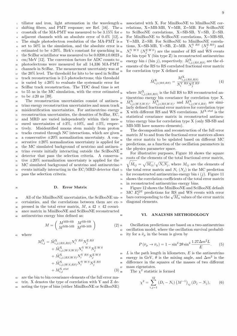
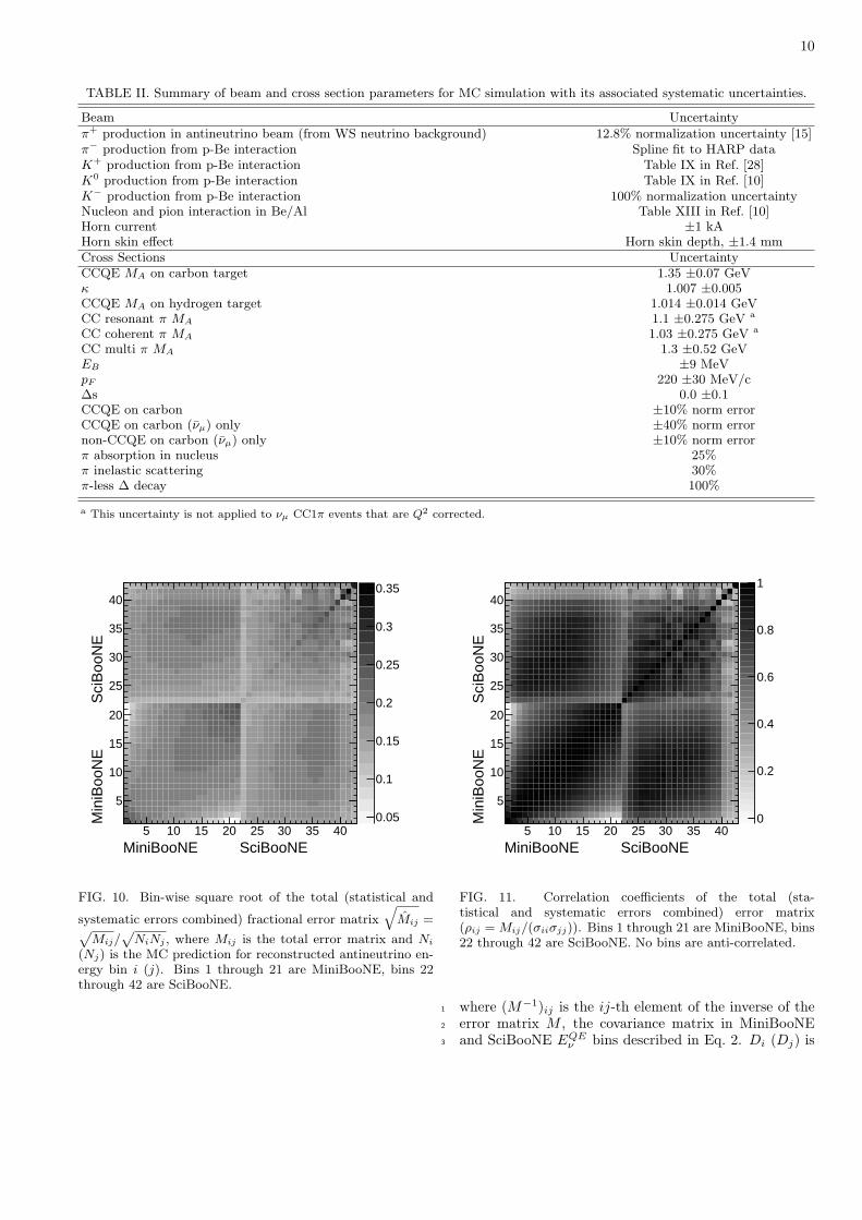
For illustrative purposes, Figure 10 shows the square69
roots of the elements of the total fractional error matrix,70 √Mij =
√Mij/
√NiNj , where Mij are the elements of71
the total error matrix and Ni (Nj) is the MC prediction72
for reconstructed antineutrino energy bin i (j). Figure 1173
shows the correlation coefficients of the total error matrix74
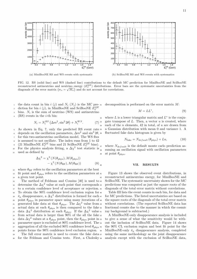
in reconstructed antineutrino energy bins.75
Figure 12 shows the MiniBooNE and SciBooNE default76
MC EQEν predictions for RS and WS events with error77
bars corresponding to the√Mii values of the error matrix78
diagonal elements.79
VI. ANALYSIS METHODOLOGY80
Oscillation predictions are based on a two-antineutrino81
oscillation model, where the oscillation survival probabil-82
ity for a νµ in the beam is given by83
P (νµ → νx) = 1− sin2 2θ sin21.27∆m2L
E. (5)
L is the path length in kilometers, E is the antineutrino84
energy in GeV, θ is the mixing angle, and ∆m2 is the85
difference in the squares of the masses of two different86
mass eigenstates.87
The χ2 statistic is formed88
χ2 =42∑
i,j=1
(Di −Ni)(M−1
)ij(Dj −Nj), (6)
10
TABLE II. Summary of beam and cross section parameters for MC simulation with its associated systematic uncertainties.
Beam Uncertaintyπ+ production in antineutrino beam (from WS neutrino background) 12.8% normalization uncertainty [15]π− production from p-Be interaction Spline fit to HARP dataK+ production from p-Be interaction Table IX in Ref. [28]K0 production from p-Be interaction Table IX in Ref. [10]K− production from p-Be interaction 100% normalization uncertaintyNucleon and pion interaction in Be/Al Table XIII in Ref. [10]Horn current ±1 kAHorn skin effect Horn skin depth, ±1.4 mmCross Sections UncertaintyCCQE MA on carbon target 1.35 ±0.07 GeVκ 1.007 ±0.005CCQE MA on hydrogen target 1.014 ±0.014 GeVCC resonant π MA 1.1 ±0.275 GeV a
CC coherent π MA 1.03 ±0.275 GeV a
CC multi π MA 1.3 ±0.52 GeVEB ±9 MeVpF 220 ±30 MeV/c∆s 0.0 ±0.1CCQE on carbon ±10% norm errorCCQE on carbon (νµ) only ±40% norm errornon-CCQE on carbon (νµ) only ±10% norm errorπ absorption in nucleus 25%π inelastic scattering 30%π-less ∆ decay 100%
a This uncertainty is not applied to νµ CC1π events that are Q2 corrected.
MiniBooNE SciBooNE 5 10 15 20 25 30 35 40
Min
iBoo
NE
S
ciB
ooN
E
5
10
15
20
25
30
35
40
0.05
0.1
0.15
0.2
0.25
0.3
0.35
FIG. 10. Bin-wise square root of the total (statistical and
systematic errors combined) fractional error matrix
√Mij =√
Mij/√
NiNj , where Mij is the total error matrix and Ni
(Nj) is the MC prediction for reconstructed antineutrino en-ergy bin i (j). Bins 1 through 21 are MiniBooNE, bins 22through 42 are SciBooNE.
MiniBooNE SciBooNE 5 10 15 20 25 30 35 40
Min
iBoo
NE
S
ciB
ooN
E
5
10
15
20
25
30
35
40
0
0.2
0.4
0.6
0.8
1
FIG. 11. Correlation coefficients of the total (sta-tistical and systematic errors combined) error matrix(ρij = Mij/(σiiσjj)). Bins 1 through 21 are MiniBooNE, bins22 through 42 are SciBooNE. No bins are anti-correlated.
where (M−1)ij is the ij-th element of the inverse of the1
error matrix M , the covariance matrix in MiniBooNE2
and SciBooNE EQEν bins described in Eq. 2. Di (Dj) is3
11
(GeV)QEnE
0.4 0.6 0.8 1 1.2 1.4 1.6 1.8
even
ts p
er b
in
0
1000
2000
3000
4000
5000
6000
(a) MiniBooNE RS and WS events with systematic
(GeV)QEnE
0.4 0.6 0.8 1 1.2 1.4 1.6 1.8
even
ts p
er b
in
0
100
200
300
400
500
600
700
800
(b) SciBooNE RS and WS events with systematics
FIG. 12. RS (solid line) and WS (dashed line) contributions to the default MC prediction for MiniBooNE and SciBooNEreconstructed antineutrino and neutrino energy (EQE
ν ) distributions. Error bars are the systematic uncertainties from thediagonals of the error matrix
(σii =
√Mii
)and do not account for correlations.
the data count in bin i (j) and Ni (Nj) is the MC pre-1
diction for bin i (j), in MiniBooNE and SciBooNE EQEν2
bins. Ni is the sum of neutrino (WS) and antineutrino3
(RS) events in the i-th bin:4
Ni = NRSi
(∆m2, sin2 2θ
)+NWS
i . (7)
As shown in Eq. 7, only the predicted RS event rate5
depends on the oscillation parameters, ∆m2 and sin2 2θ,6
for this two-antineutrino oscillation model. The WS flux7
is assumed to not oscillate. The index runs from 1 to 428
(21 MiniBooNE EQEν bins and 21 SciBooNE EQE
ν bins).9
For the physics analysis fitting, a ∆χ2 test statistic is10
used as defined by11
∆χ2 = χ2 (N(θphys),M(θphys))
− χ2 (N(θBF),M(θBF)) (8)
where θBF refers to the oscillation parameters at the best12
fit point and θphys refers to the oscillation parameters at13
a given test point.14
The method of Feldman and Cousins [40] is used to15
determine the ∆χ2 value at each point that corresponds16
to a certain confidence level of acceptance or rejection.17
To obtain the 90% confidence level exclusion region for18
νµ disappearance, a ∆χ2 distribution is formed for each19
point θphys in parameter space using many iterations of20
generated fake data at that θphys. The ∆χ2 value from21
actual data at each θphys is then compared to the fake22
data ∆χ2 distribution at each θphys. If the ∆χ2 value23
from actual data is larger than 90% of the all the fake24
data ∆χ2 values at a θphys point, then the θphys point in25
parameter space is excluded at 90% confidence level. The26
aggregation of all the excluded 90% confidence level θphys27
points forms the 90% confidence level exclusion region.28
The full error matrix is used to create the fake data29
for the Feldman and Cousins tests. First, a Cholesky30
decomposition is performed on the error matrix M :31
M = LL∗, (9)
where L is a lower triangular matrix and L∗ is the conju-32
gate transpose of L. Then, a vector u is created, where33
each of the n elements, 42 in total, of u are drawn from34
a Gaussian distribution with mean 0 and variance 1. A35
fluctuated fake data histogram is given by36
Nfake = Ndefault (θphys) + Lu, (10)
where Ndefault is the default monte carlo prediction as-37
suming an oscillation signal with oscillation parameters38
at point θphys.39
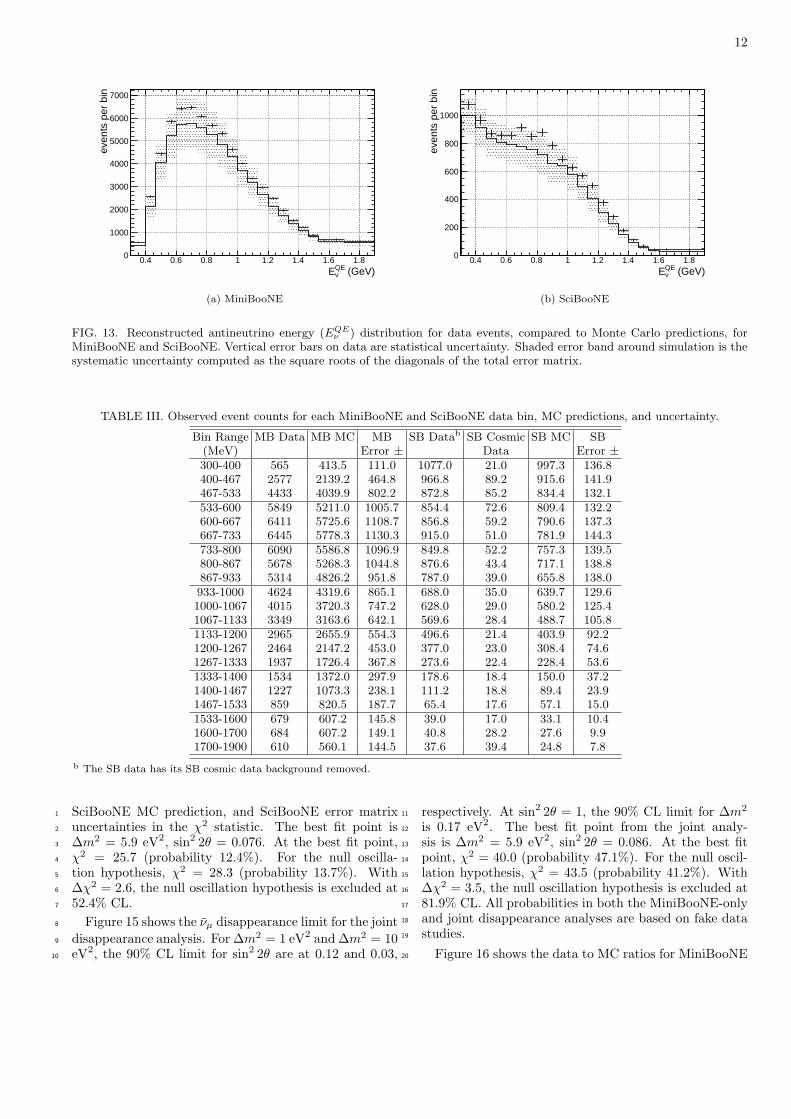
VII. RESULTS40
Figure 13 shows the observed event distributions, in41
reconstructed antineutrino energy, for MiniBooNE and42
SciBooNE. The systematic uncertainty shown for the MC43
predictions was computed as just the square roots of the44
diagonals of the total error matrix without correlations.45
Table III lists the event counts in each bin, for data and46
for MC predictions. The listed uncertainties are based on47
the square roots of the diagonals of the total error matrix48
without correlations. (The reported SciBooNE data has49
fractional counts due to the manner in which the cosmic50
ray background is subtracted.)51
A MiniBooNE-only disappearance analysis is included52
to give a sense of what the sensitivity would be with-53
out the inclusion of SciBooNE data. Figure 14 shows54
the 90% CL exclusion region and best fit point for the55
MiniBooNE-only νµ disappearance analysis, completed56
using the same methodology as the joint disappearance57
analysis except with the exclusion of SciBooNE data,58
12
(GeV)QEnE
0.4 0.6 0.8 1 1.2 1.4 1.6 1.8
even
ts p
er b
in
0
1000
2000
3000
4000
5000
6000
7000
(a) MiniBooNE
(GeV)QEnE
0.4 0.6 0.8 1 1.2 1.4 1.6 1.8
even
ts p
er b
in
0
200
400
600
800
1000
(b) SciBooNE
FIG. 13. Reconstructed antineutrino energy (EQEν ) distribution for data events, compared to Monte Carlo predictions, for
MiniBooNE and SciBooNE. Vertical error bars on data are statistical uncertainty. Shaded error band around simulation is thesystematic uncertainty computed as the square roots of the diagonals of the total error matrix.
TABLE III. Observed event counts for each MiniBooNE and SciBooNE data bin, MC predictions, and uncertainty.
Bin Range MB Data MB MC MB SB Datab SB Cosmic SB MC SB(MeV) Error ± Data Error ±300-400 565 413.5 111.0 1077.0 21.0 997.3 136.8400-467 2577 2139.2 464.8 966.8 89.2 915.6 141.9467-533 4433 4039.9 802.2 872.8 85.2 834.4 132.1533-600 5849 5211.0 1005.7 854.4 72.6 809.4 132.2600-667 6411 5725.6 1108.7 856.8 59.2 790.6 137.3667-733 6445 5778.3 1130.3 915.0 51.0 781.9 144.3733-800 6090 5586.8 1096.9 849.8 52.2 757.3 139.5800-867 5678 5268.3 1044.8 876.6 43.4 717.1 138.8867-933 5314 4826.2 951.8 787.0 39.0 655.8 138.0933-1000 4624 4319.6 865.1 688.0 35.0 639.7 129.61000-1067 4015 3720.3 747.2 628.0 29.0 580.2 125.41067-1133 3349 3163.6 642.1 569.6 28.4 488.7 105.81133-1200 2965 2655.9 554.3 496.6 21.4 403.9 92.21200-1267 2464 2147.2 453.0 377.0 23.0 308.4 74.61267-1333 1937 1726.4 367.8 273.6 22.4 228.4 53.61333-1400 1534 1372.0 297.9 178.6 18.4 150.0 37.21400-1467 1227 1073.3 238.1 111.2 18.8 89.4 23.91467-1533 859 820.5 187.7 65.4 17.6 57.1 15.01533-1600 679 607.2 145.8 39.0 17.0 33.1 10.41600-1700 684 607.2 149.1 40.8 28.2 27.6 9.91700-1900 610 560.1 144.5 37.6 39.4 24.8 7.8
b The SB data has its SB cosmic data background removed.
SciBooNE MC prediction, and SciBooNE error matrix1
uncertainties in the χ2 statistic. The best fit point is2
∆m2 = 5.9 eV2, sin2 2θ = 0.076. At the best fit point,3
χ2 = 25.7 (probability 12.4%). For the null oscilla-4
tion hypothesis, χ2 = 28.3 (probability 13.7%). With5
∆χ2 = 2.6, the null oscillation hypothesis is excluded at6
52.4% CL.7
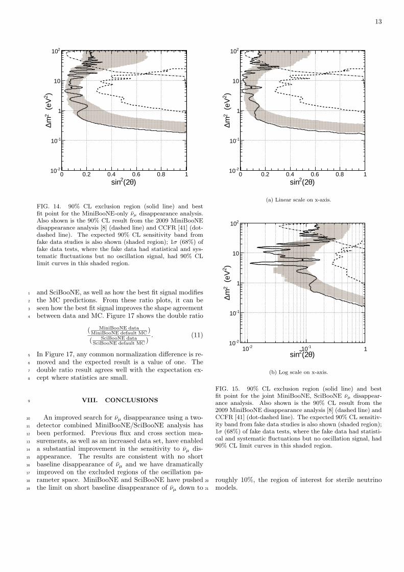
Figure 15 shows the νµ disappearance limit for the joint8
disappearance analysis. For ∆m2 = 1 eV2 and ∆m2 = 109
eV2, the 90% CL limit for sin2 2θ are at 0.12 and 0.03,10
respectively. At sin2 2θ = 1, the 90% CL limit for ∆m211
is 0.17 eV2. The best fit point from the joint analy-12
sis is ∆m2 = 5.9 eV2, sin2 2θ = 0.086. At the best fit13
point, χ2 = 40.0 (probability 47.1%). For the null oscil-14
lation hypothesis, χ2 = 43.5 (probability 41.2%). With15
∆χ2 = 3.5, the null oscillation hypothesis is excluded at16
81.9% CL. All probabilities in both the MiniBooNE-only17
and joint disappearance analyses are based on fake data18
studies.19
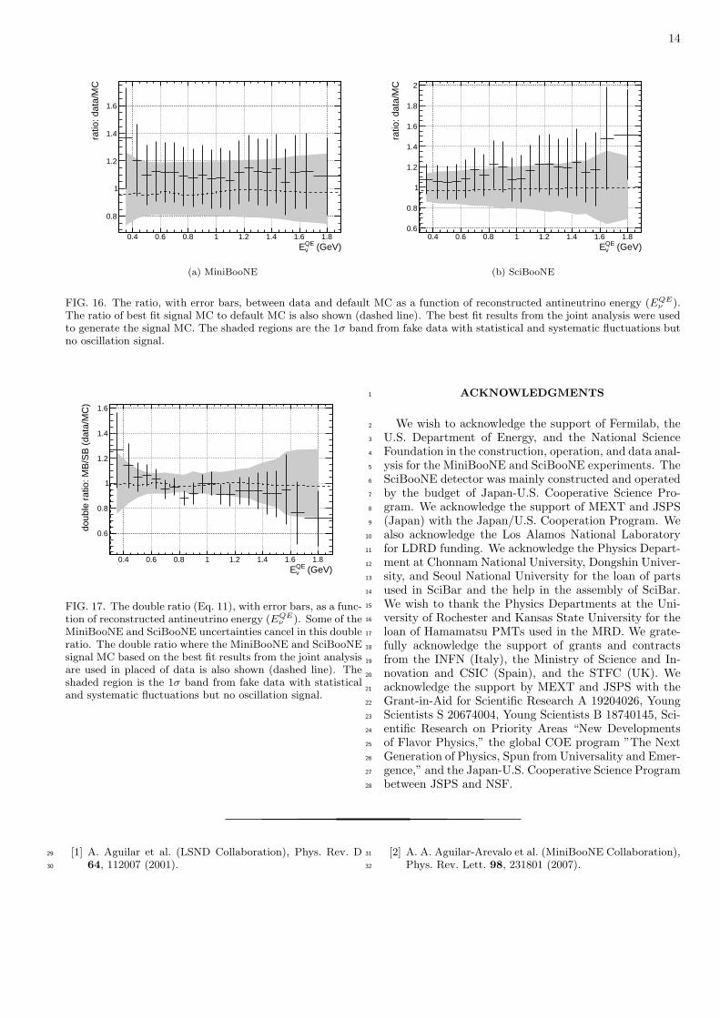
Figure 16 shows the data to MC ratios for MiniBooNE20
13
)q(22sin0 0.2 0.4 0.6 0.8 1
)2 (
eV2
mD
-210
-110
1
10
210
FIG. 14. 90% CL exclusion region (solid line) and bestfit point for the MiniBooNE-only νµ disappearance analysis.Also shown is the 90% CL result from the 2009 MiniBooNEdisappearance analysis [8] (dashed line) and CCFR [41] (dot-dashed line). The expected 90% CL sensitivity band fromfake data studies is also shown (shaded region); 1σ (68%) offake data tests, where the fake data had statistical and sys-tematic fluctuations but no oscillation signal, had 90% CLlimit curves in this shaded region.
and SciBooNE, as well as how the best fit signal modifies1
the MC predictions. From these ratio plots, it can be2
seen how the best fit signal improves the shape agreement3
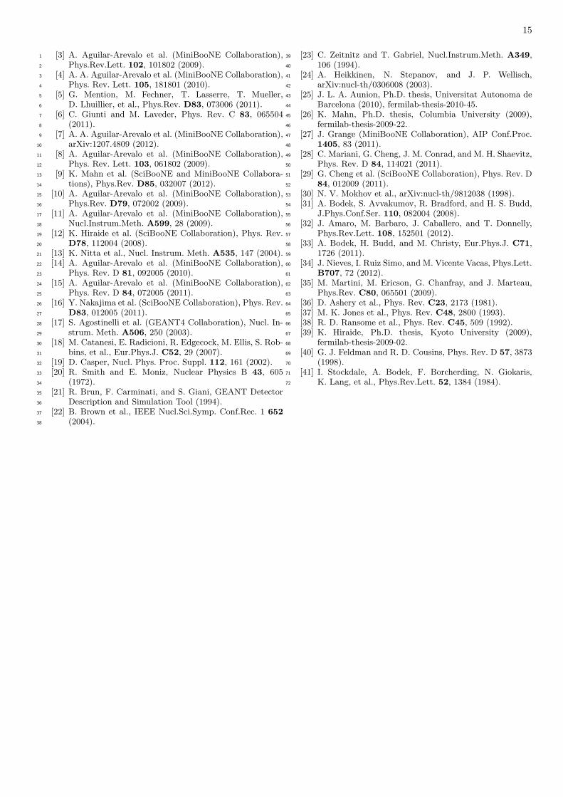
between data and MC. Figure 17 shows the double ratio4
( MiniBooNE dataMiniBooNE default MC )
( SciBooNE dataSciBooNE default MC )
. (11)
In Figure 17, any common normalization difference is re-5
moved and the expected result is a value of one. The6
double ratio result agrees well with the expectation ex-7
cept where statistics are small.8
VIII. CONCLUSIONS9
An improved search for νµ disappearance using a two-10
detector combined MiniBooNE/SciBooNE analysis has11
been performed. Previous flux and cross section mea-12
surements, as well as an increased data set, have enabled13
a substantial improvement in the sensitivity to νµ dis-14
appearance. The results are consistent with no short15
baseline disappearance of νµ and we have dramatically16
improved on the excluded regions of the oscillation pa-17
rameter space. MiniBooNE and SciBooNE have pushed18
the limit on short baseline disappearance of νµ down to19
)q(22sin0 0.2 0.4 0.6 0.8 1
)2 (
eV2
mD
-210
-110
1
10
210
(a) Linear scale on x-axis.
)q(22sin-210 -110 1
)2 (
eV2
mD
-210
-110
1
10
210
(b) Log scale on x-axis.
FIG. 15. 90% CL exclusion region (solid line) and bestfit point for the joint MiniBooNE, SciBooNE νµ disappear-ance analysis. Also shown is the 90% CL result from the2009 MiniBooNE disappearance analysis [8] (dashed line) andCCFR [41] (dot-dashed line). The expected 90% CL sensitiv-ity band from fake data studies is also shown (shaded region);1σ (68%) of fake data tests, where the fake data had statisti-cal and systematic fluctuations but no oscillation signal, had90% CL limit curves in this shaded region.
roughly 10%, the region of interest for sterile neutrino20
models.21
14
(GeV)QEnE
0.4 0.6 0.8 1 1.2 1.4 1.6 1.8
ratio
: dat
a/M
C
0.8
1
1.2
1.4
1.6
(a) MiniBooNE
(GeV)QEnE
0.4 0.6 0.8 1 1.2 1.4 1.6 1.8
ratio
: dat
a/M
C
0.6
0.8
1
1.2
1.4
1.6
1.8
2
(b) SciBooNE
FIG. 16. The ratio, with error bars, between data and default MC as a function of reconstructed antineutrino energy (EQEν ).
The ratio of best fit signal MC to default MC is also shown (dashed line). The best fit results from the joint analysis were usedto generate the signal MC. The shaded regions are the 1σ band from fake data with statistical and systematic fluctuations butno oscillation signal.
(GeV)QEnE
0.4 0.6 0.8 1 1.2 1.4 1.6 1.8
doub
le r
atio
: MB
/SB
(da
ta/M
C)
0.6
0.8
1
1.2
1.4
1.6
FIG. 17. The double ratio (Eq. 11), with error bars, as a func-tion of reconstructed antineutrino energy (EQE
ν ). Some of theMiniBooNE and SciBooNE uncertainties cancel in this doubleratio. The double ratio where the MiniBooNE and SciBooNEsignal MC based on the best fit results from the joint analysisare used in placed of data is also shown (dashed line). Theshaded region is the 1σ band from fake data with statisticaland systematic fluctuations but no oscillation signal.
ACKNOWLEDGMENTS1
We wish to acknowledge the support of Fermilab, the2
U.S. Department of Energy, and the National Science3
Foundation in the construction, operation, and data anal-4
ysis for the MiniBooNE and SciBooNE experiments. The5
SciBooNE detector was mainly constructed and operated6
by the budget of Japan-U.S. Cooperative Science Pro-7
gram. We acknowledge the support of MEXT and JSPS8
(Japan) with the Japan/U.S. Cooperation Program. We9
also acknowledge the Los Alamos National Laboratory10
for LDRD funding. We acknowledge the Physics Depart-11
ment at Chonnam National University, Dongshin Univer-12
sity, and Seoul National University for the loan of parts13
used in SciBar and the help in the assembly of SciBar.14
We wish to thank the Physics Departments at the Uni-15
versity of Rochester and Kansas State University for the16
loan of Hamamatsu PMTs used in the MRD. We grate-17
fully acknowledge the support of grants and contracts18
from the INFN (Italy), the Ministry of Science and In-19
novation and CSIC (Spain), and the STFC (UK). We20
acknowledge the support by MEXT and JSPS with the21
Grant-in-Aid for Scientific Research A 19204026, Young22
Scientists S 20674004, Young Scientists B 18740145, Sci-23
entific Research on Priority Areas “New Developments24
of Flavor Physics,” the global COE program ”The Next25
Generation of Physics, Spun from Universality and Emer-26
gence,” and the Japan-U.S. Cooperative Science Program27
between JSPS and NSF.28
[1] A. Aguilar et al. (LSND Collaboration), Phys. Rev. D29
64, 112007 (2001).30
[2] A. A. Aguilar-Arevalo et al. (MiniBooNE Collaboration),31
Phys. Rev. Lett. 98, 231801 (2007).32
15
[3] A. Aguilar-Arevalo et al. (MiniBooNE Collaboration),1
Phys.Rev.Lett. 102, 101802 (2009).2
[4] A. A. Aguilar-Arevalo et al. (MiniBooNE Collaboration),3
Phys. Rev. Lett. 105, 181801 (2010).4
[5] G. Mention, M. Fechner, T. Lasserre, T. Mueller,5
D. Lhuillier, et al., Phys.Rev. D83, 073006 (2011).6
[6] C. Giunti and M. Laveder, Phys. Rev. C 83, 0655047
(2011).8
[7] A. A. Aguilar-Arevalo et al. (MiniBooNE Collaboration),9
arXiv:1207.4809 (2012).10
[8] A. Aguilar-Arevalo et al. (MiniBooNE Collaboration),11
Phys. Rev. Lett. 103, 061802 (2009).12
[9] K. Mahn et al. (SciBooNE and MiniBooNE Collabora-13
tions), Phys.Rev. D85, 032007 (2012).14
[10] A. Aguilar-Arevalo et al. (MiniBooNE Collaboration),15
Phys.Rev. D79, 072002 (2009).16
[11] A. Aguilar-Arevalo et al. (MiniBooNE Collaboration),17
Nucl.Instrum.Meth. A599, 28 (2009).18
[12] K. Hiraide et al. (SciBooNE Collaboration), Phys. Rev.19
D78, 112004 (2008).20
[13] K. Nitta et al., Nucl. Instrum. Meth. A535, 147 (2004).21
[14] A. Aguilar-Arevalo et al. (MiniBooNE Collaboration),22
Phys. Rev. D 81, 092005 (2010).23
[15] A. Aguilar-Arevalo et al. (MiniBooNE Collaboration),24
Phys. Rev. D 84, 072005 (2011).25
[16] Y. Nakajima et al. (SciBooNE Collaboration), Phys. Rev.26
D83, 012005 (2011).27
[17] S. Agostinelli et al. (GEANT4 Collaboration), Nucl. In-28
strum. Meth. A506, 250 (2003).29
[18] M. Catanesi, E. Radicioni, R. Edgecock, M. Ellis, S. Rob-30
bins, et al., Eur.Phys.J. C52, 29 (2007).31
[19] D. Casper, Nucl. Phys. Proc. Suppl. 112, 161 (2002).32
[20] R. Smith and E. Moniz, Nuclear Physics B 43, 60533
(1972).34
[21] R. Brun, F. Carminati, and S. Giani, GEANT Detector35
Description and Simulation Tool (1994).36
[22] B. Brown et al., IEEE Nucl.Sci.Symp. Conf.Rec. 1 65237
(2004).38
[23] C. Zeitnitz and T. Gabriel, Nucl.Instrum.Meth. A349,39
106 (1994).40
[24] A. Heikkinen, N. Stepanov, and J. P. Wellisch,41
arXiv:nucl-th/0306008 (2003).42
[25] J. L. A. Aunion, Ph.D. thesis, Universitat Autonoma de43
Barcelona (2010), fermilab-thesis-2010-45.44
[26] K. Mahn, Ph.D. thesis, Columbia University (2009),45
fermilab-thesis-2009-22.46
[27] J. Grange (MiniBooNE Collaboration), AIP Conf.Proc.47
1405, 83 (2011).48
[28] C. Mariani, G. Cheng, J. M. Conrad, and M. H. Shaevitz,49
Phys. Rev. D 84, 114021 (2011).50
[29] G. Cheng et al. (SciBooNE Collaboration), Phys. Rev. D51
84, 012009 (2011).52
[30] N. V. Mokhov et al., arXiv:nucl-th/9812038 (1998).53
[31] A. Bodek, S. Avvakumov, R. Bradford, and H. S. Budd,54
J.Phys.Conf.Ser. 110, 082004 (2008).55
[32] J. Amaro, M. Barbaro, J. Caballero, and T. Donnelly,56
Phys.Rev.Lett. 108, 152501 (2012).57
[33] A. Bodek, H. Budd, and M. Christy, Eur.Phys.J. C71,58
1726 (2011).59
[34] J. Nieves, I. Ruiz Simo, and M. Vicente Vacas, Phys.Lett.60
B707, 72 (2012).61
[35] M. Martini, M. Ericson, G. Chanfray, and J. Marteau,62
Phys.Rev. C80, 065501 (2009).63
[36] D. Ashery et al., Phys. Rev. C23, 2173 (1981).64
[37] M. K. Jones et al., Phys. Rev. C48, 2800 (1993).65
[38] R. D. Ransome et al., Phys. Rev. C45, 509 (1992).66
[39] K. Hiraide, Ph.D. thesis, Kyoto University (2009),67
fermilab-thesis-2009-02.68
[40] G. J. Feldman and R. D. Cousins, Phys. Rev. D 57, 387369
(1998).70
[41] I. Stockdale, A. Bodek, F. Borcherding, N. Giokaris,71
K. Lang, et al., Phys.Rev.Lett. 52, 1384 (1984).72