This is the published version McGillivray, Mark and Pillarisetti, J. Ram 2006, Adjusting human well-being indices for gender disparity : insightful empirically, in Understanding human well-being, United Nations University Press, Tokyo, Japan, pp.169-181. Available from Deakin Research Online http://hdl.handle.net/10536/DRO/DU:30028751 Reproduced with the kind permission of the copyright owner Copyright: 2006, United Nations University Press

8

Adjusting human well-being indices for gender disparity: Insightful empirically?

Mark McGillivray and I. Ram Pillarisetti

Introduction

There has been considerable progress in recent years concerning the range and inter-country coverage of development indicators. This is par­ticularly so with what can be loosely described as social indicators. No longer are we confined to such indicators as life expectancy. literacy and mortality. Data on such indicators as the share of earned income by gen­der, parliamentary representation and access to health services are now available for reasonably large numbers of countries, both developing and developed. The UNDP has played a major role in reporting and pub­licizing these data in its Human Development Reports (HDRs, UNDP, 1990-2004). In particular, the UNDP has been a leader in combining a number of these indicators to form new composite indicators of develop­ment. Its human development index (HDI) is well known, originally ap­pearing in the HDR 1990. Since 1995 it has reported values of composites for the gender-related development index (GDI) and the gender empow­erment measure (GEM). The UNDP has been especially keen to pro­mote the GDI and the GEM, and made gender aspects of development the main focus of its HDR 1995.

Development clearly fails (or cannot be said to have occurred) if its fruits are not equitably distributed between females and males. The GDI and GEM are thus important contributions by emphasizing gender issues in development. Yet at a purely empirical level there is reason to ques­tion the insightfulness of these new indices. Research conducted by Hicks

169

170 McGILLIVRAY AND PILLARISETTI

and Streeten (1979), Larson and Wilford (1979), McGillivray (1991), McGillivray and White (1993), Srinivasan (1994) and Cahill (2005) has shown that social and composite indicators of development tend to be very highly correlated with income per capita. On the basis of this out­come it has often been concluded that these indicators, at best, offer lim­ited additional empirical insights into inter-country development levels or, at worst, are empirically redundant. This finding is especially pointed in the case of composite indicators, as they have often been devised to move attention away from income per capita by revealing insights that they cannot. l Should we draw similar conclusions for the GDI and GEM? That is, do they provide insights into inter-country development levels that pre-existing indicators cannot?2

This is the issue to which the current chapter turns. Specifically, it looks at the extent to which the GEM and GDI provide information. that non-gender-specific indicators cannot provide. It is especially inter­ested in whether these indicators tell us more than the HD I can alone tell us. It should be stressed that the chapter does not question the ideo­logical basis of the GDI and GEM, nor their roles in bringing attention to gender issues or in mobilizing effort to reduce gender imbalances. The non-gender-specific indicators under consideration are income per capita (measured using PPP GDP) and the HDI. A range of simple yet insight­ful and powerful parametric and non-parametric statistical tests are em­ployed. Unlike most other studies the chapter also considers explicitly the statistical basis on which an indicator is deemed non-insightful or re­dundant.

The GDI and GEM

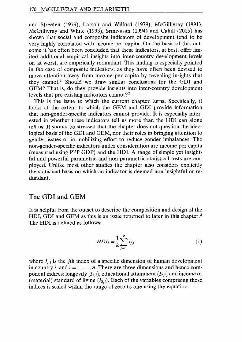
It is helpful from the outset to describe the composition and design of the HDI, GDI and GEM as this is an issue returned to later in this chapter. 3

The HD I is defined as follows:

1 k HDL =-'" L· I kL J,l

j=l

(1)

where Ij,i is the jth index of a specific dimension of human development in country i, and i = I, ... ,n. There are three dimensions and hence com­ponent indices: longevity (h,i), educational attainment (lz) and income or (material) standard of living (h,i)' Each of the variables comprising these indices is scaled within the range of zero to one using the equation:

ADJUSTING INDICES FOR GENDER DISPARITY 171

X. . - X min X . . _ ],k,l j,k

], I - X max _ X min j,k j,k

(2)

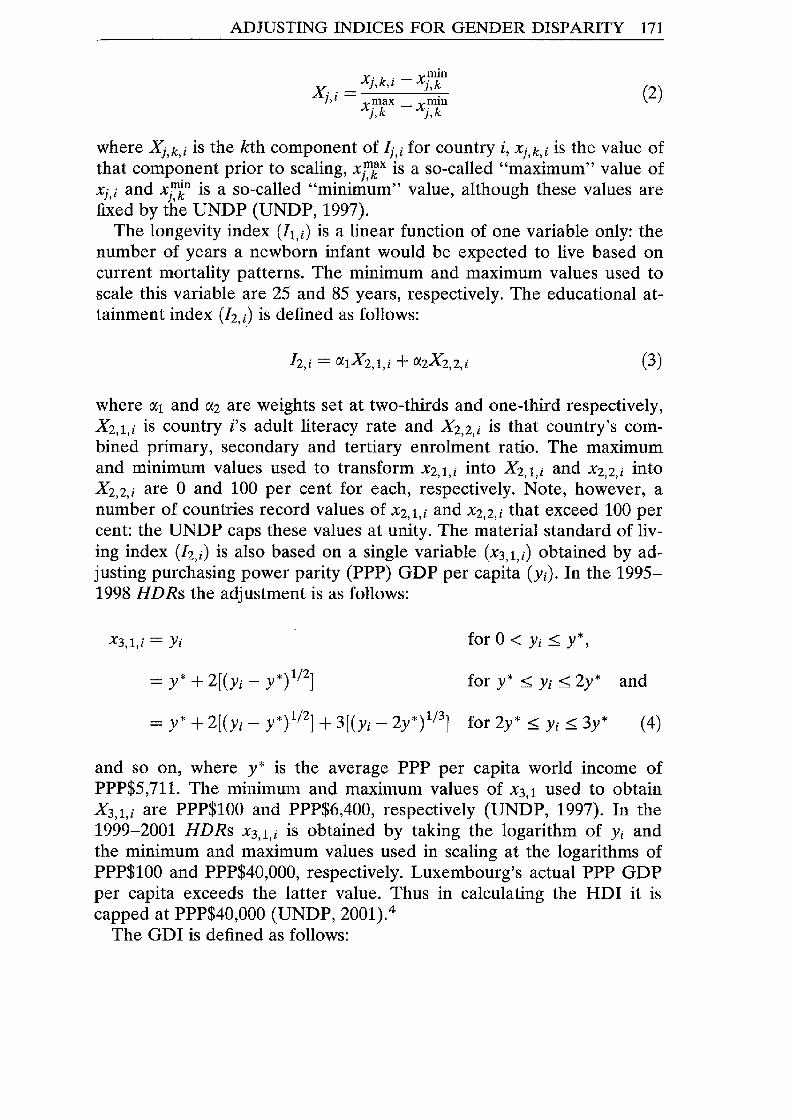
where Xj,k,i is the kth component of Ij,; for country i, Xj,k,i is the value of that comp~nent prior to scaling, Xj~:x is a so-called "maximum" value of Xj,; and xrt is a so-called "minimum" value, although these values are fixed by the UNDP (UNDP, 1997).

The longevity index CIt,i) is a linear function of one variable only: the number of years a newborn infant would be expected to live based on current mortality patterns. The minimum and maximum values used to scale this variable are 25 and 85 years, respectively. The educational at­tainment index (h,l) is defined as follows:

12 . = !XIX2 1 . + !X2X 2 2 . ,l , ,l , ,l (3)

where !Xl and !X2 are weights set at two-thirds and one-third respectively, X2,I,; is country i's adult literacy rate and X2,2,i is that country's com­bined primary, secondary and tertiary enrolment ratio. The maximum and minimum values used to transform X2 1 ; into X2 1 i and X2 2 i into , , , , 1 ,

X 2, 2, i are ° and 100 per cent for each, respectively. Note, however, a number of countries record values of X2,1,i and X2,2,i that exceed 100 per cent: the UNDP caps these values at unity. The material standard of liv­ing index (h,i) is also based on a single variable (X3,I,i) obtained by ad­justing purchasing power parity (PPP) GDP per capita (Yi). In the 1995-1998 HDRs the adjustment is as follows:

X3,1,i = Yi for 0 < Yi < y*,

= y* + 2[(Yi - y*)1/2] for y* < Yi < 2y* and

= y* + 2[(Yi - y*)1/2] + 3[(Yi - 2y*)1/3] for 2y* < Yi < 3y* (4)

and so on, where y* is the average PPP per capita world income of PPP$5,711. The minimum and maximum values of x3 1 used to obtain , X3,1,i are PPP$100 and PPP$6,400, respectively (UNDP, 1997). In the 1999-2001 HDRs X3,1,i is obtained by taking the logarithm of Yi and the minimum and maximum values used in scaling at the logarithms of PPP$100 and PPP$40,OOO, respectively. Luxembourg's actual PPP GDP per capita exceeds the latter value. Thus in calculating the HDI it is capped at PPP$40,000 (UNDP, 2001).4

The GDI is defined as follows:

172 McGILLIVRAY AND PILLARISETTI

1 k GDIi = -" Ir k~ J,I

j=l

(5)

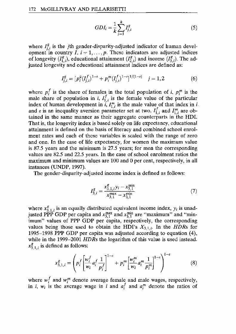
where Ili is the jth gender-disparity-adjusted indicator of human devel­opment in country I, i = 1, ... , p. These indicators are adjusted indices of longevity (If.i)' educational attainment (Iti) and income (If.J The ad­justed longevity and educational attainment indices are defined as:

I? = [ ~(I/.)l-e + p'!I (I!.) l-e] 1f{1-e) J,I PI "I I "I

j= 1,2 (6)

where p{ is the share of females in the total population of i, pi is the male share of population in i, If i is the female value of the particular index of human development in i: Iii is the male value of that index in i, and e is an inequality aversion para~eter set at two. If i and Iii are ob­tained in the same manner as their aggregate counterparts in the HDI. That is, the longevity index is based solely on life expectancy, educational attainment is defined on the basis of literacy and combined school enrol­ment rates and each of these variables is scaled with the range of zero and one. In the case of life expectancy, for women the maximum value is 87.5 years and the minimum is 27.5 years; for men the corresponding values are 82.5 and 22.5 years. In the case of school enrolment ratios the maximum and minimum values are 100 and 0 per cent, respectively, in all instances (UNDP, 1997).

The gender-disparity-adjusted income index is defined as follows:

g min ]g _ X3, 1,iYi - X3,1

3, i - Xmax _ X min 3,1 3,1

(7)

where x~ 1 i is an equally distributed equivalent income index, Yi is unad-, , . J'usted PPP GDP per capita and x max and xmm are "maximum" and "min-3,1 3,1 imum" values of PPP GDP per capita, respectively, the corresponding values being those used to obtain the HDI's X 3,1,i. In'the HDRs for 1995-1998 PPP GDP per capita was adjusted according to equation (4), while in the 1999-2001 HDRs the logarithm of this value is used instead. x~ 1 i is defined as follows: , ,

(

1

)

l-e f -e m l-e

x3g 1 . = pt [Wi at 1t] + p'!l [~a'!l ~l

' ,1 I W. I I W. I pm 1 Pi I i

(8)

where w{ and wf" denote average female and male wages, respectively, in i, Wi is the average wage in i and a{ and af" denote the ratios of

ADJUSTING INDICES FOR GENDER DISPARITY 173

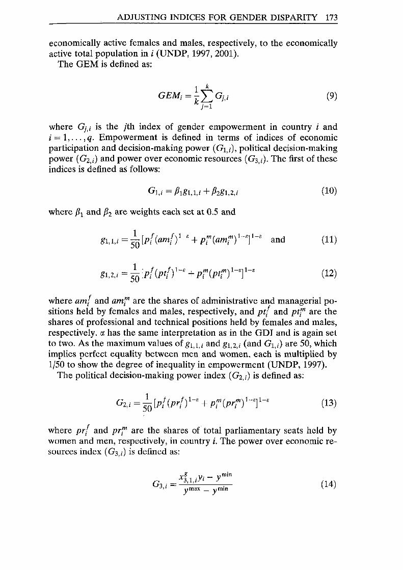
economically active females and males, respectively, to the economically active total population in i (UNDP, 1997, 2001).

The GEM is defined as:

1 k GEM, = - '" G· . I kL...t j,l

j=l

(9)

where Gj,i is the jth index of gender empowerment in country i and i = 1, ... , q. Empowerment is defined in terms of indices of economic participation and decision-making power (Gl,i), political decision-making power (G2,i) and power over economic resources (G3,i). The first of these indices is defined as follows:

(10)

where PI and P2 are weights each set at 0.5 and

1 [/( I)l-e m(' m)l-e]l-e d gl,l,i = 50 Pi ami + Pi ami an (11)

(12)

where am! and ami are the shares of administrative and managerial po­sitions held by females and males, respectively, and pt! and pti are the shares of professional and technical positions held by females and males, respectively. IX has the same interpretation as in the GDI and is again set to two. As the maximum values of gl,l,i and gl,2,i (and G1,i) are 50, which implies perfect equality between men and women, each is mUltiplied by 1/50 to show the degree of inequality in empowerment (UNDP, 1997).

The political decision-making power index (G2,i) is defined as:

(13)

where pr! and pri are the shares of total parliamentary seats held by women and men, respectively, in country i. The power over economic re­sources index (G3,i) is defined as:

x g 'Yi - ymin G ,= _3--,-, --,-1, _I __ -:--

3,1 max min y - y (14)

174 McGILLIVRA Y AND PILLARISETTI

where ymin and ymax are the minimum and maximum values of actual PPP GDP per capita, respectively. The corresponding values used by the UNDP are PPP$100 and PPP$40,000 respectively (UNDP, 1997). >

Data and statistical methods

Data are taken from the HDR 2001 (UNDP, 2001). Three samples are employed, each determined by data availability: a sample of 174 coun­tries for which data on the HDI and income per capita are available; a sample of 148 countries for which data on income per capita and the HDI and GDI are available; and a sample of 102 countries for which data on each of income per capita and the HDI, GDI and GEM are avail­able. Each of these samples is divided into subsamples defined according to whether a country is classified as high human development, medium human development, low human development, high income, medium income or low income. Country classifications are available in UNDP (2001). Most of the data used to calculate index values relate to 1999 (UNDP, 2001).

Three test statistics were utilized: the Pearson zero-order correlation coefficient; the Spearman rank-order correlation coefficient; and the Ken­dall tau-beta coefficient. The use and interpretation of these coefficients require elaboration. Of issue here is the level of these coefficients which deems the new indicator sufficiently insightful for it not to be redundant. Srinivasan (1994) reminds us that there are two extremes in assessing whether an indicator provides additional statistical information as com­pared to others. An indicator will provide no more information than an­other if they are perfectly correlated with each other. In this case the new indicator is perfectly redundant with respect to the other. At the other extreme, the new insights are at a maximum if the two indicators are mu­tually orthogonal. It follows that one can test for the perfect redundancy of an indicator by evaluating the null hypothesis that the particular coef­ficient's value is one. Failure to reject is evidence of perfect redundancy. In practice, however, this test will almost always be passed.

A more appropriate question is whether the extent of redundancy jus­tifies the effort involved in calculating and reporting the new indicator. This involves a threshold to differentiate between redundancy and non­redundancy. McGillivray and White (1993) provide two thresholds -0.90 and 0.70 - and hence evaluate the nulls that the particular coefficient equates to these values, which are termed as type I and type II redun­dancy respectively. These thresholds are of course arbitrary, but would appear to be reasonable. The current chapter therefore evaluates the fol­lowing hypotheses:

ADJUSTING INDICES FOR GENDER DISPARITY 175

• HJ: p > 0.90 • Hi: p < 0.90 and • HJI: p > 0.70 • HP: p < 0.70 where p is the chosen coefficient of statistical association. The null hy­pothesis, in each case, is of redundancy, either types I or II. The chapter also evaluates the null of perfect redundancy, that the coefficient is equal to one.

Results

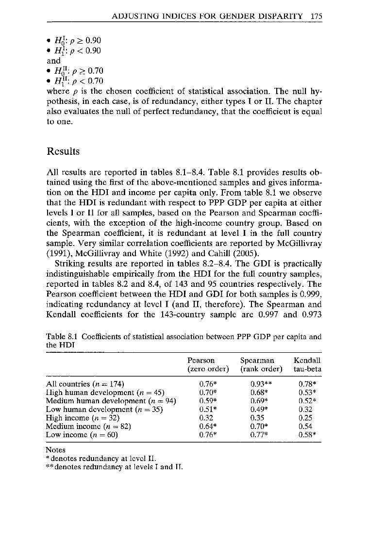
All results are reported in tables 8.1-8.4. Table 8.1 provides results ob­tained using the first of the above-mentioned samples and gives informa­tion on the HDI and income per capita only. From table 8.1 we observe that the HDI is redundant with respect to PPP GDP per capita at either levels I or II for all samples, based on the Pearson and Spearman coeffi­cients, with the exception of the high-income country group. Based on the Spearman coefficient, it is redundant at level I in the full country sample. Very similar correlation coefficients are reported by McGillivray (1991), McGillivray and White (1992) and Cahill (2005).

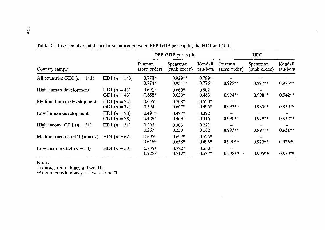
Striking results are reported in tables 8.2-8.4. The GDI is practically indistinguishable empirically from the HDI for the full country samples, reported in tables 8.2 and 8.4, of 143 and 95 countries respectively. The Pearson coefficient between the HDI and GDI for both samples is 0.999, indicating redundancy at level I (and II, therefore). The Spearman and Kendall coefficients for the 143-country sample are 0.997 and 0.973

Table 8.1 Coefficients of statistical association between PPP GDP per capita and the HDI

All countries (n = 174) High human development (n = 45) Medium human development (n = 94) Low human development (n = 35) High income (n = 32) Medium income (n = 82) Low income (n = 60)

Notes * denotes redundancy at level II. ** denotes redundancy at levels I and II.

Pearson (zero order)

0.76* 0.70* 0.59* 0.51* 0.32 0.64* 0.76*

Spearman Kendall (rank order) tau-beta

0.93** 0.68* 0.69* 0.49* 0.35 0.70* 0.77*

0.78* 0.53* 0.52* 0.32 0.25 0.54 0.58*

~ --...l 0\

Table 8.2 Coefficients of statistical association between PPP GDP per capita, the HDI and GDI

PPP GDP per capita HDI

Pearson Spearman Kendall Pearson Spearman Kendall Country sample (zero order) (rank order) tau-beta (zero order) (rank order) tau-beta

All countries GDI (n = 143) HDI (n = 143) 0.778* 0.939** 0.789* 0.774* 0.931** 0.776* 0.999** 0.997** 0.973**

High human development HDI (n = 43) 0.691* 0.660* 0.502 GDI (n = 43) 0.658* 0.623* 0.463 0.994** 0.990** 0.942**

Medium human development HDI (n = 72) 0.635* 0.708* 0.530* GDI (n = 72) 0.594* 0.667* 0.495* 0.993** 0.983** 0.929**

Low human development HDI (n = 28) 0.491* 0.477* 0.322 GDI (n = 28) 0.488* 0.463* 0.316 0.990** 0.979** 0.912**

High income GDI (n = 31) HDI (n = 31) 0.296 0.303 0.222 0.267 0.250 0.182 0.993** 0.997** 0.931 **

Medium income GDI (n = 62) HDI (n = 62) 0.695* 0.692* 0.525* 0.646* 0.658* 0.496* 0.990** 0.979** 0.926**

Low income GDI (n = 50) HDI (n = 50) 0.735* 0.722* 0.550* 0.728* 0.712* 0.537* 0.998** 0.995** 0.959**

Notes * denotes redundancy at level II. ** denotes redundancy at levels I and II.

ADJUSTING INDICES FOR GENDER DISPARITY 177

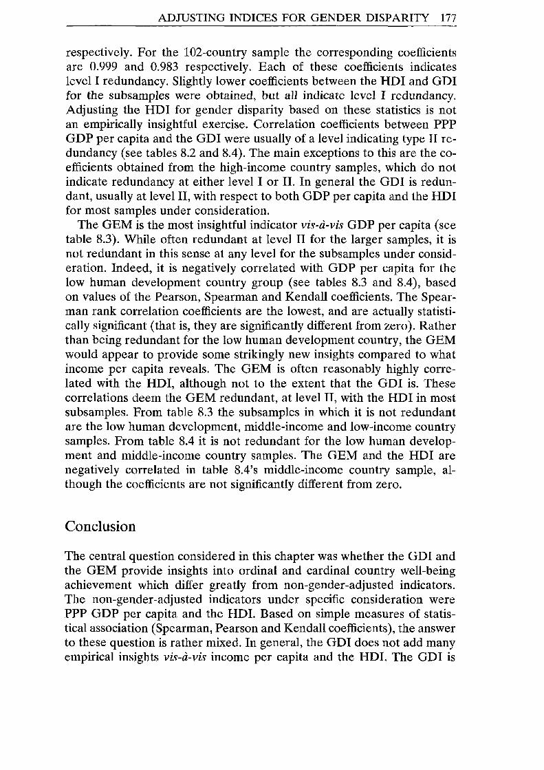
respectively. For the 102-country sample the corresponding coefficients are 0.999 and 0.983 respectively. Each of these coefficients indicates level I redundancy. Slightly lower coefficients between the HDI and GDI for the subsamples were obtained, but all indicate level I redundancy. Adjusting the HDI for gender disparity based on these statistics is not an empirically insightful exercise. Correlation coefficients between PPP GDP per capita and the GDI were usually of a level indicating type II re­dundancy (see tables 8.2 and 8.4). The main exceptions to this are the co­efficients obtained from the high-income country samples, which do not indicate redundancy at either level I or II. In general the GDI is redun­dant, usually at level II, with respect to both GDP per capita and the HDI for most samples under consideration.

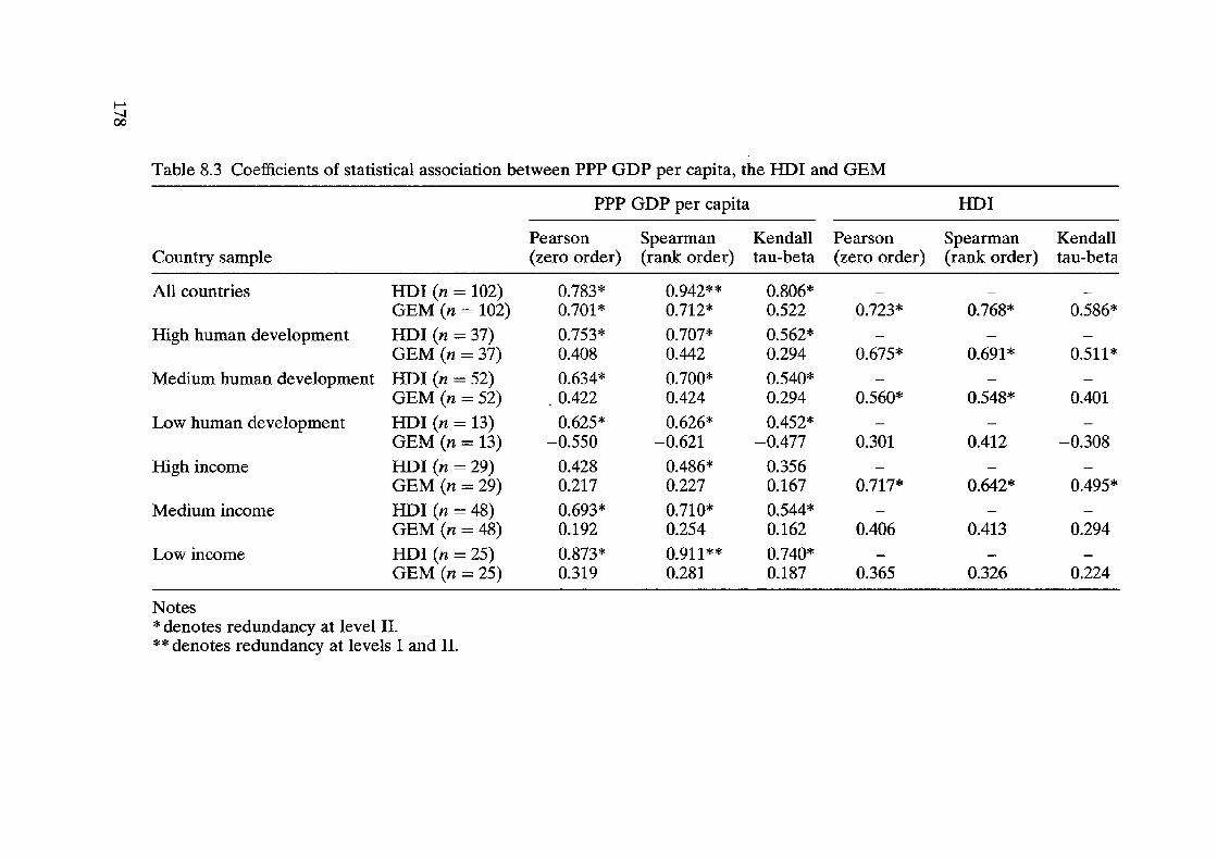
The GEM is the most insightful indicator vis-a-vis GDP per capita (see table 8.3). While often redundant at level II for the larger samples, it is not redundant in this sense at any level for the sUbsamples under consid­eration. Indeed, it is negatively correlated with GDP per capita for the low human development country group (see tables 8.3 and 8.4), based on values of the Pearson, Spearman and Kendall coefficients. The Spear­man rank correlation coefficients are the lowest, and are actually statisti­cally significant (that is, they are significantly different from zero). Rather than being redundant for the low human development country, the GEM would appear to provide some strikingly new insights compared to what income per capita reveals. The GEM is often reasonably highly corre­lated with the HDI, although not to the extent that the GDI is. These correlations deem the GEM redundant, at level II, with the HDI in most subsamples. From table 8.3 the subsamples in which it is not redundant are the low human development, middle-income and low-income country samples. From table 8.4 it is not redundant for the low human develop­ment and middle-income country samples. The GEM and the HDI are negatively correlated in table 8.4's middle-income country sample, al­though the coefficients are not significantly different from zero.

Conclusion

The central question considered in this chapter was whether the GDI and the GEM provide insights into ordinal and cardinal country well-being achievement which differ greatly from non-gender-adjusted indicators. The non-gender-adjusted indicators under specific consideration were PPP GDP per capita and the HDI. Based on simple measures of statis­tical association (Spearman, Pearson and Kendall coefficients), the answer to these question is rather mixed. In general, the GDI does not add many empirical insights vis-a-vis income per capita and the HDI. The GDI is

I--' -....} 00

Table 8.3 Coefficients of statistical association between PPP GDP per capita, the HDI and GEM

PPP GDP per capita HDI

Pearson Spearman Kendall Pearson Spearman Kendall Country sample (zero order) (rank order) tau-beta (zero order) (rank order) tau-beta

All countries HDI (n = 102) 0.783* 0.942** 0.806* GEM (n = 102) 0.701* 0.712* 0.522 0.723* 0.768* 0.586*

High human development HDI (n = 37) 0.753* 0.707* 0.562* GEM (n = 37) 0.408 0.442 0.294 0.675* 0.691* 0.511 *

Medium human development HDI (n = 52) 0.634* 0.700* 0.540* GEM (n = 52) 0.422 0.424 0.294 0.560* 0.548* 0.401

Low human development HDI (n = 13) 0.625* 0.626* 0.452* GEM (n = 13) -0.550 -0.621 -0.477 0.301 0.412 -0.308

High income HDI (n = 29) 0.428 0.486* 0.356 GEM (n = 29) 0.217 0.227 0.167 0.717* 0.642* 0.495*

Medium income HDI (n = 48) 0.693* 0.710* 0.544* GEM (n = 48) 0.192 0.254 0.162 0.406 0.413 0.294

Low income HDI (n = 25) 0.873* 0.911** 0.740* GEM (n = 25) 0.319 0.281 0.187 0.365 0.326 0.224

Notes * denotes redundancy at level II. ** denotes redundancy at levels I and II.

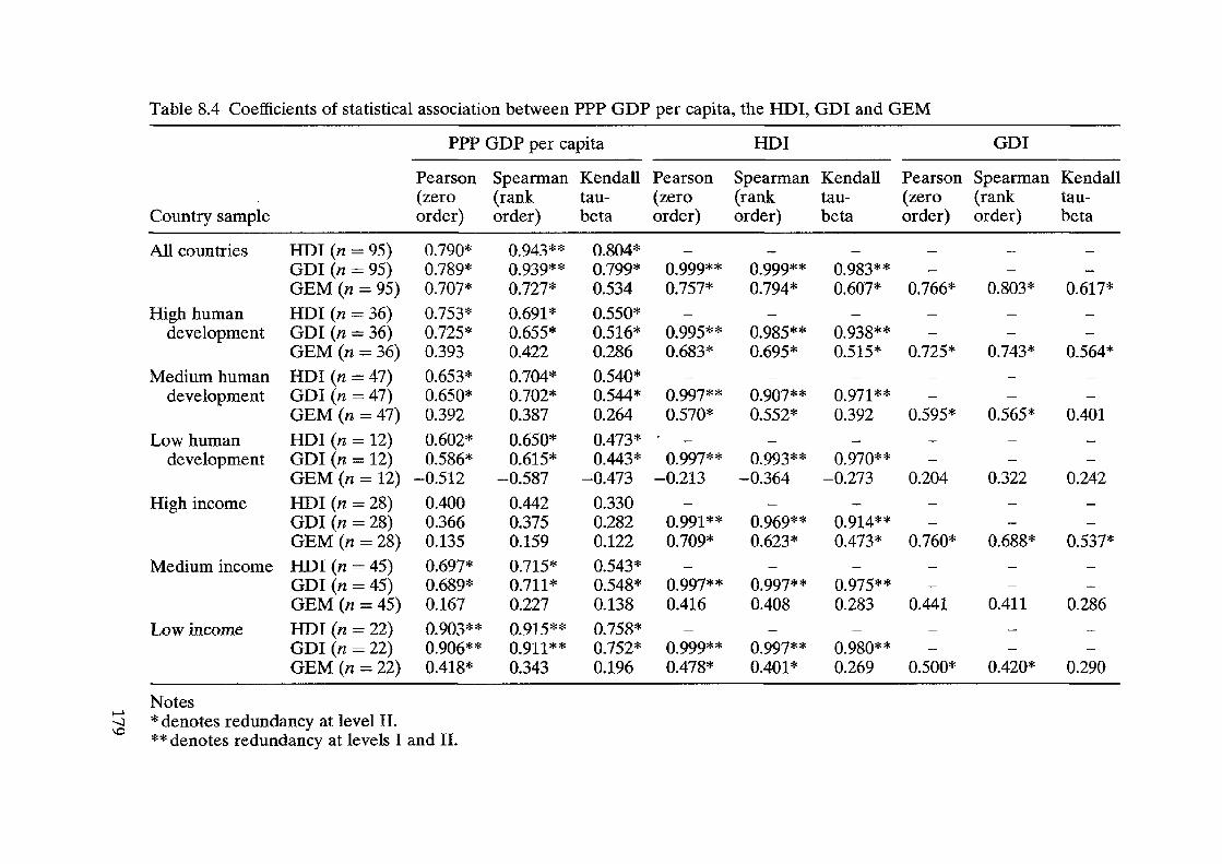
Table 8.4 Coefficients of statistical association between PPP GDP per capita, the HDI, GDI and GEM

PPP GDP per capita HDI GDI

Pearson Spearman Kendall Pearson Spearman Kendall Pearson Spearman Kendall (zero (rank tau- (zero (rank tau- (zero (rank tau-

Country sample order) order) beta order) order) beta order) order) beta

All countries HDI (n = 95) 0.790* 0.943** 0.804* GDI (n = 95) 0.789* 0.939** 0.799* 0.999** 0.999** 0.983** GEM (n = 95) 0.707* 0.727* 0.534 0.757* 0.794* 0.607* 0.766* 0.803* 0.617*

High human HDI (n = 36) 0.753* 0.691* 0.550* development GDI (n = 36) 0.725* 0.655* 0.516* 0.995** 0.985** 0.938**

GEM (n = 36) 0.393 0.422 0.286 0.683* 0.695* 0.515* 0.725* 0.743* 0.564*

Medium human HDI (n = 47) 0.653* 0.704* 0.540* development GDI (n = 47) 0.650* 0.702* 0.544* 0.997** 0.907** 0.971 **

GEM (n = 47) 0.392 0.387 0.264 0.570* 0.552* 0.392 0.595* 0.565* 0.401

Low human HOI (n = 12) 0.602* 0.650* 0.473* development GOI (n = 12) 0.586* 0.615* 0.443* 0.997** 0.993** 0.970**

GEM (n = 12) -0.512 -0.587 -0.473 -0.213 -0.364 -0.273 0.204 0.322 0.242

High income HOI (n = 28) 0.400 0.442 0.330 GOI (n = 28) 0.366 0.375 0.282 0.991** 0.969** 0.914** GEM (n = 28) 0.135 0.159 0.122 0.709* 0.623* 0.473* 0.760* 0.688* 0.537*

Medium income HDI (n = 45) 0.697* 0.715* 0.543* GDI (n = 45) 0.689* 0.711* 0.548* 0.997** 0.997** 0.975** GEM (n = 45) 0.167 0.227 0.138 0.416 0.408 0.283 0.441 0.411 0.286

Low income HOI (n = 22) 0.903** 0.915** 0.758* GDI (n = 22) 0.906** 0.911 ** 0.752* 0.999** 0.997** 0.980** GEM (n = 22) 0.418* 0.343 0.196 0.478* 00401 * 0.269 0.500* 0.420* 0.290

Notes f-' * denotes redundancy at level II. -.....l \0

** denotes redundancy at levels I and II.

180 McGILLIVRA Y AND PILLARISETTI

practically indistinguishable empirically from the HDI for larger samples of countries. Adjusting the HDI for gender disparity adds little empiri­cally, it seems. The GEM offers more original insights than the GDI, es­pecially for country subsamples, in which is can be negatively correlated with both income per capita and the HDI. Evidence is thus mixed on whether adjusting well-being indicators for gender disparity matters empirically - in some instances it does and in others it does not. This does not, however, diminish the conceptual and ideological case for such adjustments. From a practitioner or policy-maker perspective, it follows that if they want to use a national-level gender-adjusted development in­dicator that provides different information to the HDI, the GEM is pref­erable to the GDI.

Notes

1. Note that this finding has not stopped the UNDP and others from making claims to the contrary. Typically these claims are based on comparing extreme cases where a country's rank based on one indicator differs radically from that generated by another, rather than on large samples of countries.

2. Saith and Harriss-White (1999) also ask this question, based on the findings of McGilliv­ray (1991) and McGillivray and White (1992), but do not pursue it empirically.

3. While the aim of this chapter is not to critique the UNDP's indicators, it is not blind to the various limitations identified in the literature. Relevant studies include Dasgupta (1990), McGillivray (1991), McGillivray and White (1992), Ogwang (1994), Gormely (1995), Streeten (1995), Hicks (1997), Ivanova, Arcelus and Srinivasan (1998), Sagar and Najam (1998), Noorbakhsh (1998a, 1998b), Pillarisetti and McGillivray (1998), Bard­han and Klasen (1999), Saith and Harriss-White (1999), Neumayer (2001) and Morse (2003). One should not forget these limitations, and the various caveats emerging from them, in interpreting the results reported here.

4. See Anand and Sen (2000) for an excellent discussion of income in the HDI.

REFERENCES

Anand, S. and A. Sen (2000) "The Income Component of the Human Develop­ment Index", Journal of Human Development 1: 83-106.

Bardhan, K. and S. Klasen (1999) "UNDP's Gender-related Indices: A Critical Review", World Development 27: 985-1010.

Cahill, M. (2005) "Is the Human Development Index Redundant?", Eastern Eco­nomic Journal 31: 1-5.

Dasgupta, P. (1990) "Well-being in Poor Countries", Economic and Political Weekly, 4 August: 1713-1720.

Gormely, P. J. (1995) "The Human Development Index in 1994: Impact of In­come on Country Rank", Journal of Economic and Social Measurement 21: 253-267.

ADJUSTING INDICES FOR GENDER DISPARITY 181

Hicks, D. A. (1997) "The Inequality Adjusted Human Development Index: A Constructive Proposal", World Development 25: 1283-1298.

Hicks, N. and P. Streeten (1979) "Indicators of Development: The Search for a Basic Needs Yardstick", World Development 7: 567-580.

Ivanova, I., F. 1. Arcelus and G. Srinivasan (1998) "An Assessment of the Mea­surement Properties of the Human Development Index", Social Indicators Re­search 46: 157-179.

Larson, D. A. and W. T. Wilford (1979) "The Physical Quality of Life Index: A Useful Social Indicator?", World Development 7: 581-584.

McGillivray, M. (1991) "The Human Development Index: Yet Another Redun­dant Composite Development Indicator?", World Development 19: 1451-1460.

McGillivray, M. and H. White (1992) "Measuring Development? A Statistical Critique of the Human Development Index", Working Paper 135, Institute of Social Studies, The Hague.

~~- (1993) "Measuring Development? The UNDP's Human Development In­dex", Journal of International Development 5: 183-192.

Morse, S. (2003) "For Better or For Worse, Till the Human Development Index Do Us Part?", Ecological Economics 45: 281-296.

Neumayer, E. (2001) "The Human Development Index and Sustainability - A Constructive Proposal", Ecological Economics 39: 101-114.

Noorbakhsh, F. (1998a) "A Modified Human Development Index", World Devel­opment 26: 517-528.

~-- (1998b) "A Human Development Index: Some Technical Issues and Al­ternative Indices", Journal of International Development 10: 589-605.

Ogwang, T. (1994) "The Choice of Principal Variables for Computing the Human Development Index", World Development 22: 2011-2114.

Pillarisetti, J. R. and M. McGillivray (1998) "Human Development and Gender Empowerment", Development Policy Review 16: 197-203.

Sagar, A. and A. Najam (1998) "The Human Development Index: A Critical Re­view", Ecological Economics 25: 249-264.

Saith, R. and B. Harriss-White (1999) "The Gender Sensitivity of Well-being In­dicators", Development and Change 30: 465-498.

Srinivasan, T. N. (1994) "Human Development: A New Paradigm or Reinvention of the Wheel?", American Economic Review Papers and Proceedings 84: 238-243.

Streeten, P. (1995) "Human Development: The Debate about the Index", Inter­national Social Science Journal 47: 25-37.

UNDP (1990-2004) Human Development Report, New York: Oxford University Press.