Embed Size (px)
Citation preview
AGC
DSP
1
An Introductory Course
D. Mandic and L. Arnaut [email protected], [email protected]
URL: www.commsp.ee.ic.ac.uk/~mandic
(based on the notes by Prof. A G Constantinides)
AGC
DSP
2
Contents
1- Introduction
2 - FIR filters
3 - IIR filters
4 Frequency transforms and DFT
5 - Multirate processing
6 – Estimation theory
7 – Least squares and prediction problem
8 – Case studies

AGC
DSP
3
BOOKS !! Main Course text books: Digital Signal Processing:
A computer Based Approach, S K Mitra, McGraw Hill
!! Mathematical Methods and Algorithms for Signal Processing, Todd Moon, Addison Wesley
!! Other books:
!! Digital Signal Processing, Roberts & Mullis, Addison Wesley
!! Digital Filters, Antoniou, McGraw Hill
AGC
DSP
4
Analogue Vs Digital Signal Processing
Reliability:
Analogue system performance degrades due to:
• Long term drift (ageing)
• Short term drift (temperature?)
• Sensitivity to voltage instability.
• Batch-to-Batch component variation.
• High discrete component count
Interconnection failures
AGC
DSP
5
Digital Systems:
• No short or long term drifts.
• Relative immunity to minor power supply variations.
• Virtually identical components.
• IC’s have > 15 year lifetime
• Development costs
• System changes at design/development stage only software changes.
• Digital system simulation is realistic.
Power aspects
!! Size, Dissipation
!! DSP chips available as well as ASIC/FPGA realisations
AGC
DSP
6
Radar systems & Sonar systems
• Doppler filters.
• Clutter Suppression.
• Matched filters.
• Target tracking.
!! Identification

AGC
DSP
7
Image Processing
!! Image data compression.
!! Image filtering.
!! Image enhancement.
!! Spectral Analysis.
!! Scene Analysis / Pattern recognition.
AGC
DSP
8
Biomedical Signal Analysis
!! Spatial image enhancement. (X-rays)
!! Spectral Analysis.
!! 3-D reconstruction from projections.
!! Digital filtering and Data compression.

AGC
DSP
9
Music
!! Music recording.
!! Multi-track “mixing”.
!! CD and DAT.
!! Filtering / Synthesis / Special effects.
AGC
DSP
10
Seismic Signal Analysis
!! Bandpass Filtering for S/N improvement.
!! Predictive deconvolution to extract reverberation characteristics.
!! Optimal filtering. (Wiener and Kalman.)

AGC
DSP
11
Telecommunications and Consumer Products
These are the largest and most pervasive applications of DSP and Digital Filtering
!! Mobile Communications
!! Digital Recording
!! Digital Cameras
!! Blue Tooth or similar
Based on notes by Dr Tania Stathaki

What is a signal ?
A signal is a function of an independent
variable such as time, distance, position,
temperature, pressure, etc.
For example…
•! Electrical Engineering
voltages/currents in a circuit
speech signals
image signals
•! Physics
radiation
•! Mechanical Engineering
vibration studies
•! Astronomy
space photos

or
•!Biomedicine EEG, ECG, MRI, X-Rays, Ultrasounds
•!Seismology tectonic plate movement, earthquake prediction
•!Economics
stock market data

What is DSP?
Mathematical and algorithmic manipulation of discretized and
quantized or naturally digital signals in order to extract the most
relevant and pertinent information that is carried by the signal.
What is a signal?
What is a system?
What is processing?
Signals can be characterized in several ways
Continuous time signals vs. discrete time signals (x(t), x[n]). Temperature in London / signal on a CD-ROM.
Continuous valued signals vs. discrete signals. Amount of current drawn by a device / average scores of TOEFL in a school
over years.
–Continuous time and continuous valued : Analog signal.
–Continuous time and discrete valued: Quantized signal.
–Discrete time and continuous valued: Sampled signal.
–Discrete time and discrete values: Digital signal.
Real valued signals vs. complex valued signals. Resident use electric power / industrial use reactive power.
Scalar signals vs. vector valued (multi-channel) signals. Blood pressure signal / 128 channel EEG.
Deterministic vs. random signal: Recorded audio / noise.
One-dimensional vs. two dimensional vs. multidimensional signals. Speech / still image / video.

Systems
•! For our purposes, a DSP system is one that can mathematically
manipulate (e.g., change, record, transmit, transform) digital
signals.
•! Furthermore, we are not interested in processing analog signals
either, even though most signals in nature are analog signals.

Filtering
•! By far the most commonly used DSP operation Filtering refers to deliberately changing the frequency content of the
signal, typically, by removing certain frequencies from the signals.
For de-noising applications, the (frequency) filter removes those frequencies in the signal that correspond to noise.
In various applications, filtering is used to focus to that part of the spectrum that is of interest, that is, the part that carries the information.
•! Typically we have the following types of filters Low-pass (LPF) –removes high frequencies, and retains (passes) low
frequencies.
High-pass (HPF) –removes low frequencies, and retains high frequencies.
Band-pass (BPF) –retains an interval of frequencies within a band, removes others.
Band-stop (BSF) –removes an interval of frequencies within a band, retains others.
Notch filter –removes a specific frequency.
A Common Application: Filtering

Components of a DSP System
Components of a DSP System

Components of a DSP System
Analog-to-Digital-to-Analog…? •! Why not just process the signals in continuous time domain? Isn’t it just a waste of time,
money and resources to convert to digital and back to analog?
•! Why DSP? We digitally process the signals in discrete domain, because it is
–! !More flexible, more accurate, easier to mass produce. More flexible, more accurate, easier to mass produce.
–! !Easier to design. Easier to design.
• System characteristics can easily be changed by programming.
• Any level of accuracy can be obtained by use of appropriate number
of bits.
–! !More deterministic and reproducible-less sensitive to component values, More deterministic and reproducible-less sensitive to component values,
etc.
–! !Many things that cannot be done using analog processors can be done Many things that cannot be done using analog processors can be done
digitally.
• Allows multiplexing, time sharing, multi-channel processing, adaptive filtering.
• Easy to cascade, no loading effects, signals can be stored indefinitely w/o loss.
• Allows processing of very low frequency signals, which requires unpractical
component values in analog world.
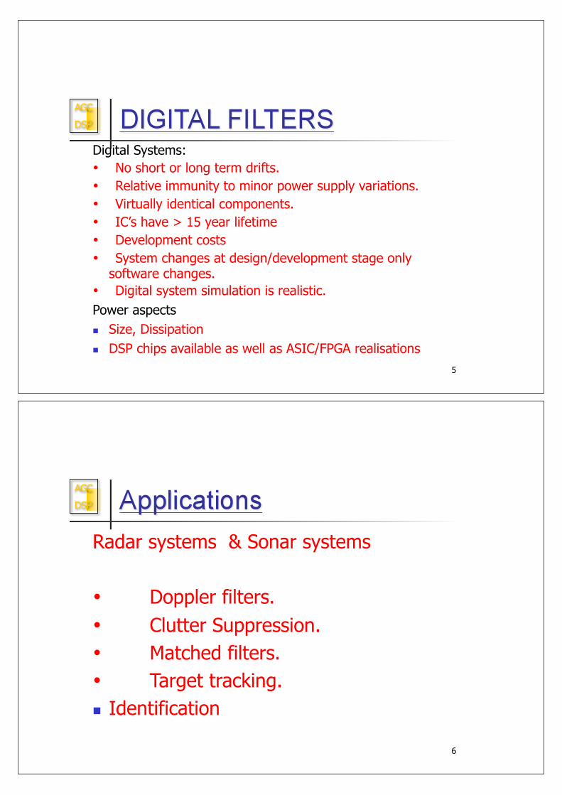
Analog-to-Digital-to-Analog…?
•!On the other hand, it can be
–!!Slower, sampling issues. Slower, sampling issues.
–!!More expensive, increased system More expensive, increased system
complexity,
consumes more power.
•!Yet, the advantages far outweigh the
disadvantages. Today, most continuous time
signals are in fact processed in discrete time
using digital signal processors.
Analog-Digital
Examples of analog technology
•! photocopiers
•! telephones
•! audio tapes
•! televisions (intensity and color info per scan line)
•! VCRs (same as TV)
Examples of digital technology
•! Digital computers!

256x256 64x64
2 Dimensions
From Continuous to Discrete: Sampling
256x256 256 levels 256x256 32 levels
Discrete (Sampled) and Digital (Quantized) Image

256x256 256 levels 256x256 2 levels
Discrete (Sampled) and Digital (Quantized) Image
•! Employed to generate a new sequence y[n]
with a sampling rate higher or lower
than that of the sampling rate of a given
sequence x[n]
•! Sampling rate alteration ratio is
•! If R > 1, the process called interpolation
•! If R < 1, the process called decimation

•! In up-sampling by an integer factor L > 1,
equidistant zero-valued samples are
inserted by the up-sampler between each
two consecutive samples of the input
sequence x[n]:
L
•!An example of the up-sampling operation
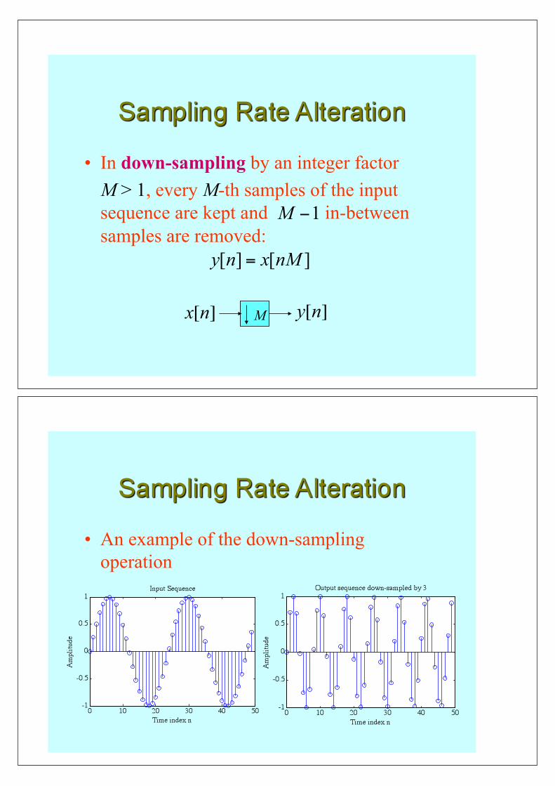
•! In down-sampling by an integer factor
M > 1, every M-th samples of the input
sequence are kept and in-between
samples are removed:
M
•!An example of the down-sampling
operation

AGC
DSP
Professor A G Constantinides© 1
BACKGROUND: Signal Spaces
!! The purpose of this part of the course is to introduce
the basic concepts behind generalised Fourier
Analysis
!! The approach is taken via vector spaces and least
squares approximation
!! Modern Signal Processing is based in a substantial
way on the theory of vector spaces. In this course we
shall be concerned with the discrete–time case only
AGC
DSP
Professor A G Constantinides© 2
Signal Spaces
!! In order to compare two signals we need to define a measure of “distance” known as a metric.
!! A metric is a function that produces a scalar value from two signals such that
!! 1)
!! 2)
!! 3)
!! 4)

AGC
DSP
Professor A G Constantinides© 3
Signal Spaces
!! There are many metrics that can be used.
!! Examples:
!! 1) If we have a set of finite numbers representing
signals then a metric may be
!! This is known as the metric or the Manhattan
distance.
AGC
DSP
Professor A G Constantinides© 4
Signal Spaces
!! 2) Another metric for the same set is
This is called the metric or the Euclidean distance
!! 3) Yet another form is the metric

AGC
DSP
Professor A G Constantinides© 5
Signal Spaces
!! 4) As the integer the last form becomes
This is called the metric or distance.
!! In channel coding we use the Hamming Distance as a metric
where is the modulo-2 addition of two binary vectors
AGC
DSP
Professor A G Constantinides© 6
Signal Spaces
!! When the set of vectors which we use is defined
along with an appropriate metric then we say we
have a metric space.
!! There are many metric spaces as seen from the
earlier discussion on metrics.
!! (In the case of continuous time signals we say we
have function spaces)

AGC
DSP
Professor A G Constantinides© 7
Vector Spaces
!! We think of a vector as an assembly of elements
arranged as
!! The length may be in certain cases infinite
AGC
DSP
Professor A G Constantinides© 8
Vector Spaces
!! A linear vector space S over a set of scalars R is formed when a collection of vectors is taken together with an addition operation and a scalar multiplication, and satisfies the following:
!! 1) S is a group under addition ie the following are satisfied
!! a) for any and in S then is also in S
!! b) there is a zero identity element ie
!! c) for every element there is another such that their sum is zero
!! d) addition is associative ie

AGC
DSP
Professor A G Constantinides© 9
Vector Spaces
!! 2) For any pair of scalars and
!! 3) There is a unit element in the set of scalars R such that
(The set of scalars is usually taken as the set of real numbers)
AGC
DSP
Professor A G Constantinides© 10
Linear Combination
!! Often we think of a signal as being composed of
other simpler (or more convenient to deal with)
signals. The simplest composition is a linear combination of the form
!! Where are the simpler
signals, and the coefficients are in the scalar set.

AGC
DSP
Professor A G Constantinides© 11
Vector space …
AGC
DSP
Professor A G Constantinides© 12
Vector space …

AGC
DSP
Professor A G Constantinides© 13
Linear Independence
!! If there is no nonzero set of coefficients
such that
then we say that the set of vectors
is linearly dependent
AGC
DSP
Professor A G Constantinides© 14
Linear Independence
!! Examples:
!! 1)
Observe that
ie the set is linearly dependent
AGC
DSP
Professor A G Constantinides© 15
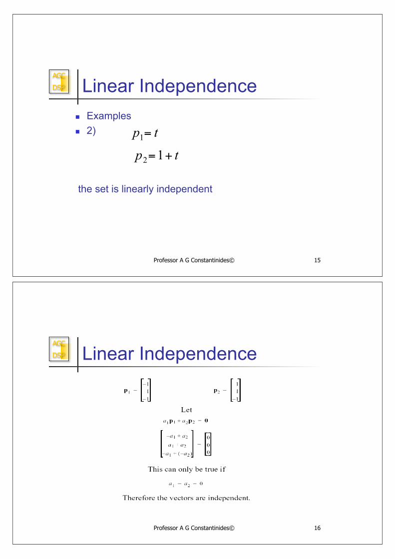
Linear Independence
!! Examples
!! 2)
the set is linearly independent
AGC
DSP
Professor A G Constantinides© 16
Linear Independence

AGC
DSP
Professor A G Constantinides© 17
The Span of Vectors
!! The Span of a vector set is the set of all possible
vectors that can be reached (ie made through linear
combinations) from the given set.
!! That is there exists a set
such that
AGC
DSP
Professor A G Constantinides© 18
The Span of Vectors
!! Example: The vectors below are in 3-D real vector
space.
!! Their linear combination forms
which is essentially a vector in the plane of the
given two vectors.

AGC
DSP
Professor A G Constantinides© 19
Basis and Dimension
!! If is a selection of
linearly independent vectors from a vector space
such that they span the entire space then we say the selected vectors form a (complete) basis.
!! The number of elements in the basis is the cardinality
of the basis
!! The least number of independent vectors to span a
given vector space is called the dimension of the
vector space, usually designated as
AGC
DSP
Professor A G Constantinides© 20
IMPORTANT!
!! Every vector space has a basis.
!! Thus for many purposes whatever operations we want to do in the vector space can be done with the basis.

AGC
DSP
Professor A G Constantinides© 21
Basis
AGC
DSP
Professor A G Constantinides© 22
Vector Spaces
!! Let us start with the intuitive notion that we can represent a signal as
!! This representation is called a projection of ,the signal, into the linear vector space
!! The vectors above are linearly independent and can span any signal in the space

AGC
DSP
Professor A G Constantinides© 23
Vector Spaces
!! Examples are seen in Matrix Theory and typically in
Fourier Analysis.
!! The length of a vector is known as the norm.
!! We can select any convenient norm, but for
mathematical tractability and convenience we select
the second order norm.
!! A real valued function is the norm of
AGC
DSP
Professor A G Constantinides© 24
Norm
!! A real valued function is the norm of when it
satisfies
!! Positivity
!! Zero length
!! Scaling
!! Triangle inequality

AGC
DSP
Professor A G Constantinides© 25
Induced norm/Cauchy
Schwartz inequality
!! Induced norm of the space follows from the inner
product as
!! The norm is represented as
!! The following condition (Cauchy-Schwartz) is
satisfied by an induced norm (eg )
AGC
DSP
Professor A G Constantinides© 26
Inner Product
!! The inner product of two vectors in a scalar, and has
the following properties
!!
!! if the vectors are real then
!!
AGC
DSP
Professor A G Constantinides© 27
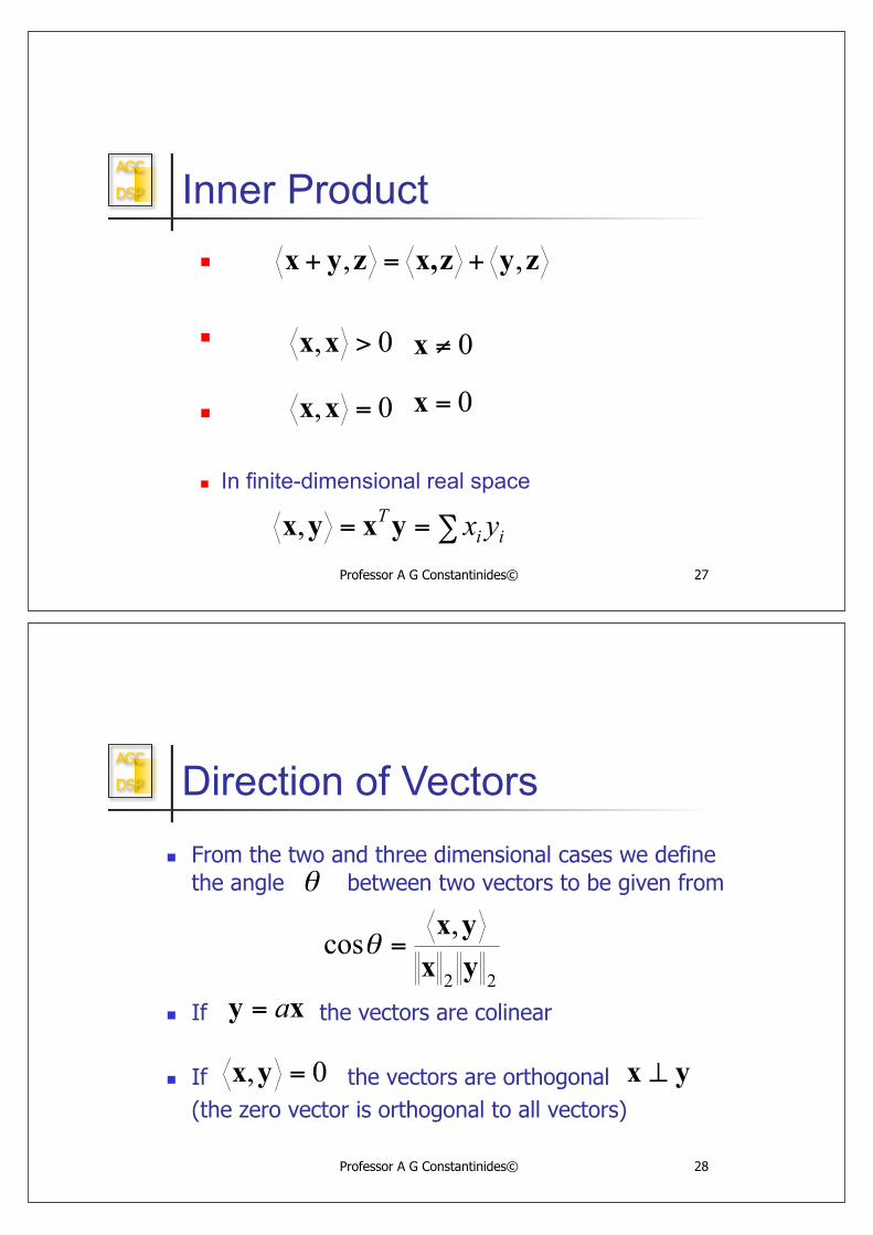
Inner Product
!!
!!
!!
!! In finite-dimensional real space
AGC
DSP
Professor A G Constantinides© 28
Direction of Vectors
!! From the two and three dimensional cases we define the angle between two vectors to be given from
!! If the vectors are colinear
!! If the vectors are orthogonal
(the zero vector is orthogonal to all vectors)

AGC
DSP
Professor A G Constantinides© 29
Orthonormal
!! A set of vectors is
orthonormal when
!! (Pythagoras)
If then the indiced norms satisfy
AGC
DSP
Professor A G Constantinides© 30
Weighted inner product
!! Very often we want a weighted inner product which we define as
where is a Hermitian matrix
For the induced norm to be positive for we must have for all non-zero vectors
This means that must be positive definite

AGC
DSP
Professor A G Constantinides© 31
Example
!! Let
!! Clearly
!! while
AGC
DSP
Professor A G Constantinides© 32
Example
!! Note that the inner product in the previous example
cannot serve as a norm as for any
we have
!! This violates the conditions for a norm

AGC
DSP
Professor A G Constantinides© 33
Complete spaces
!! If every signal in a signal space is reachable (ie can
be spanned) by a set of vectors then the space is
complete and the reaching a complete set
!! This means that there will be no left over part of a
given signal expressed as an appropriate linear
combination of basis vectors
!! For example a Fourier series reaches all periodic
signals in the least square sense, and hence the set
of all complex exponentials is a complete set
AGC
DSP
Professor A G Constantinides© 34
Hilbert spaces
!! Complete linear vector spaces with induced
norms are known as Hilbert Spaces
!! In signal processing we are mainly interested in finite
energy signals ie in Hilbert spaces
!! If the norm above is orther than the second then we
have Banach Spaces. (Such norms are useful in approximating signals and system functions as we
shall see later)
AGC
DSP
Professor A G Constantinides© 35
Orthogonal subspaces
!! Let S be a inner product signal (vector) space and V
and W be subspaces of S.
!! Then V and W are orthogonal if for every
and we have
!! In above the set of all vectors orthogonal to a
subspace is called the orthogonal complement of the of the subspace denoted by
AGC
DSP
Professor A G Constantinides© 36
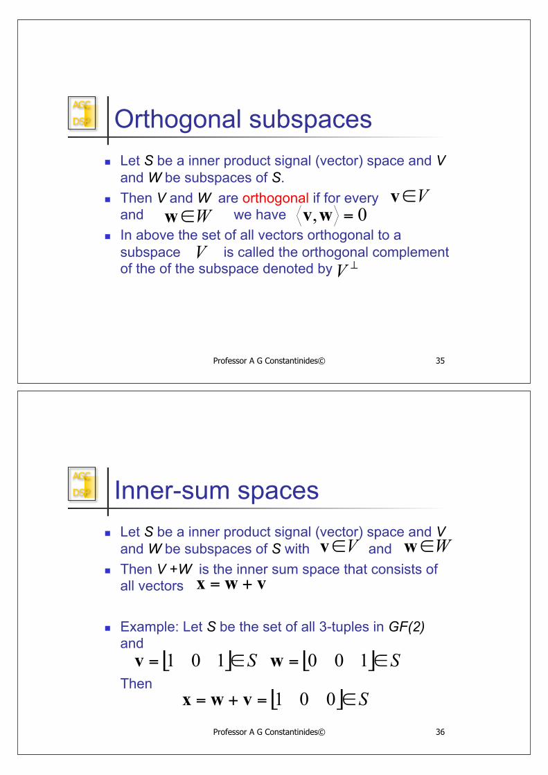
Inner-sum spaces
!! Let S be a inner product signal (vector) space and V
and W be subspaces of S with and
!! Then V +W is the inner sum space that consists of
all vectors
!! Example: Let S be the set of all 3-tuples in GF(2)
and
Then
AGC
DSP
Professor A G Constantinides© 37
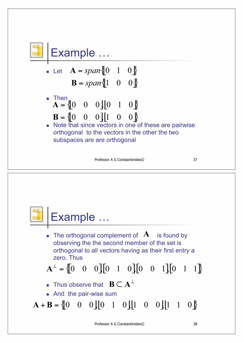
Example …
!! Let
!! Then
!! Note that since vectors in one of these are pairwise
orthogonal to the vectors in the other the two
subspaces are are orthogonal
AGC
DSP
Professor A G Constantinides© 38
Example …
!! The orthogonal complement of is found by
observing the the second member of the set is
orthogonal to all vectors having as their first entry a zero. Thus
!! Thus observe that
!! And the pair-wise sum

AGC
DSP
Professor A G Constantinides© 39
Disjoint spaces
!! If two linear vector spaces of the same dimensionality
have only the zero vector in common they are called
disjoint.
!! Two disjoint spaces are such that one is the algebraic
complement of the other
!! Their sum is the entire vector space
AGC
DSP
Professor A G Constantinides© 40
Disjoint spaces …
!! Let S be a inner product signal (vector) space and V and W be subspaces of S
!! Then for every there exist unique vectors
such that
if and only if the two sbspaces are disjoint.
(ie if they are not disjoint a vector may be generated form a pair-wise sum of more than one pair)

AGC
DSP
Professor A G Constantinides© 41
Projections
!! From above a pictorial representation can be
produced as
AGC
DSP
Professor A G Constantinides© 42
Projections
!! Let S be a inner product signal (vector) space and V
and W be subspaces of S
!! We can think of and as being the
projections of in the component sets.
!! We introduce the projection operator
such that for any we have
!! That is the operation returns that component of
that lies in V

AGC
DSP
Professor A G Constantinides© 43
Projections
"! Thus if is already in V the operation does not change the value of
"! Thus
"! This gives us the definition
A linear tranformation is a projection if
(Idempotent operator)
AGC
DSP
Professor A G Constantinides© 1
BACKGROUND: Hilbert Spaces
Linear Transformations and Least Squares:
Hilbert Spaces

AGC
DSP
Professor A G Constantinides© 2
Linear Transformations
!! A transformation from a vector space to a vector space with the same scalar field denoted by
is linear when
!!
!! Where
!! We can think of the transformation as an operator
AGC
DSP
Professor A G Constantinides© 3
Linear Transformations …
!! Example: Mapping a vector space from to
can be expressed as a mxn matrix.
!! Thus the transformation
can be written as
AGC
DSP
Professor A G Constantinides© 4
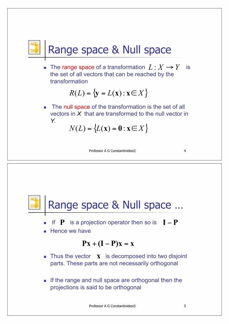
Range space & Null space
!! The range space of a transformation is
the set of all vectors that can be reached by the
transformation
!! The null space of the transformation is the set of all
vectors in X that are transformed to the null vector in
Y.
AGC
DSP
Professor A G Constantinides© 5
Range space & Null space …
!! If is a projection operator then so is
!! Hence we have
!! Thus the vector is decomposed into two disjoint
parts. These parts are not necessarily orthogonal
!! If the range and null space are orthogonal then the
projections is said to be orthogonal

AGC
DSP
Professor A G Constantinides© 6
Linear Transformations
!! Example: Let
and let the transformation a nxm matrix
Then
Thus, the range of the linear transformation (or column space of the matrix ) is the span of the basis vectors.
The null space is the set which yields
AGC
DSP
Professor A G Constantinides© 7
A Problem
!! Given a signal vector in the vector space S, we
want to find a point in the subset V of the space ,
nearest to

AGC
DSP
Professor A G Constantinides© 8
A Problem …
!! Let us agree that “nearest to” in the figure is taken in the Euclidean distance sense.
!! The projection orthogonal to the set V gives the desired solution.
!! Moreover the error of representation is
!! This vector is clearly orthogonal to the set V (More on this later)
AGC
DSP
Professor A G Constantinides© 9
Another perspective …
!! We can look at the above problem as seeking to find
a solution to the set of linear equations
where the given vector is not in the range of
as is the case with an overspecified set of equations.
!! There is no exact solution. If we project orthogonally
the given vector into the range of then we have
the “shortest norm solution” in terms of the Euclidean
distance of the “error”.
AGC
DSP
Professor A G Constantinides© 10
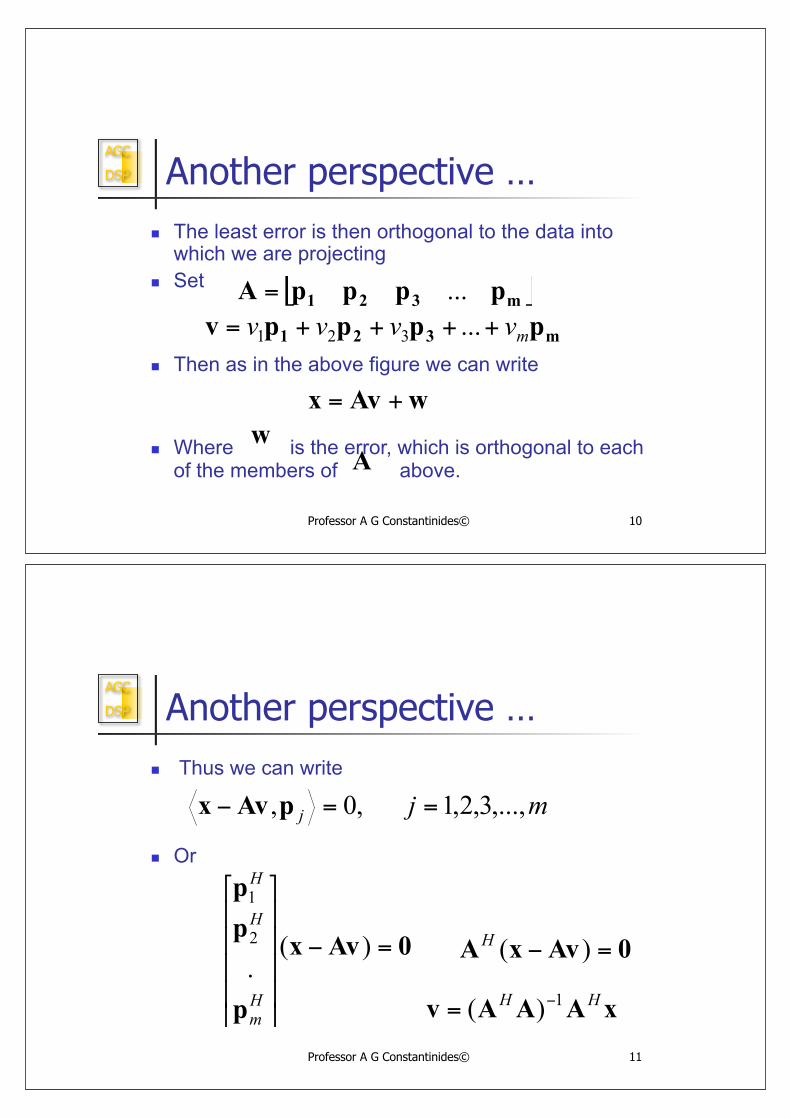
Another perspective …
!! The least error is then orthogonal to the data into which we are projecting
!! Set
!! Then as in the above figure we can write
!! Where is the error, which is orthogonal to each of the members of above.
AGC
DSP
Professor A G Constantinides© 11
Another perspective …
!! Thus we can write
!! Or

AGC
DSP
Professor A G Constantinides© 12
Another perspective …
!! Thus
and hence the projection matrix is
ie this is the matrix that projects orthogonally into
the column space of
AGC
DSP
Professor A G Constantinides© 13
Another perspective …
!! If we adopt the weighted form
!! The induced norm is
!! Then the projection matrix is
!! Where is positive definite

AGC
DSP
Professor A G Constantinides© 14
Least Squares Projection
PROJECTION THEOREM
In a Hilbert space the orthogonal projection of a
signal into a smaller dimensional space minimises the
norm of the error, and the error vector is orthogonal to
the data (ie the smaller dimensional space).
AGC
DSP
Professor A G Constantinides© 15
Orthogonality Principle
!! Let be a set of
independent vectors in a vector space S.
!! We wish to express any vector in S as
!! If is in the span of the independent vectors then
the representation will be exact.
!! If on the other hand it is not then there will be an
error

AGC
DSP
Professor A G Constantinides© 16
Orthogonality Principle
!! In the latter case we can write
!! Where
is an approximation to given vector with error
!! We wish to find that approximation which minimises
the Euclidean error norm (squared)
AGC
DSP
Professor A G Constantinides© 17
Orthogonality Principle
!! Expand to
!! Where

AGC
DSP
Professor A G Constantinides© 18
Reminders
AGC
DSP
Professor A G Constantinides© 19
Orthogonality Principle
!! On setting this to zero we obtain the solution
!! This is a minimum because on differentiating we
have a positive definite matrix
AGC
DSP
Professor A G Constantinides© 20
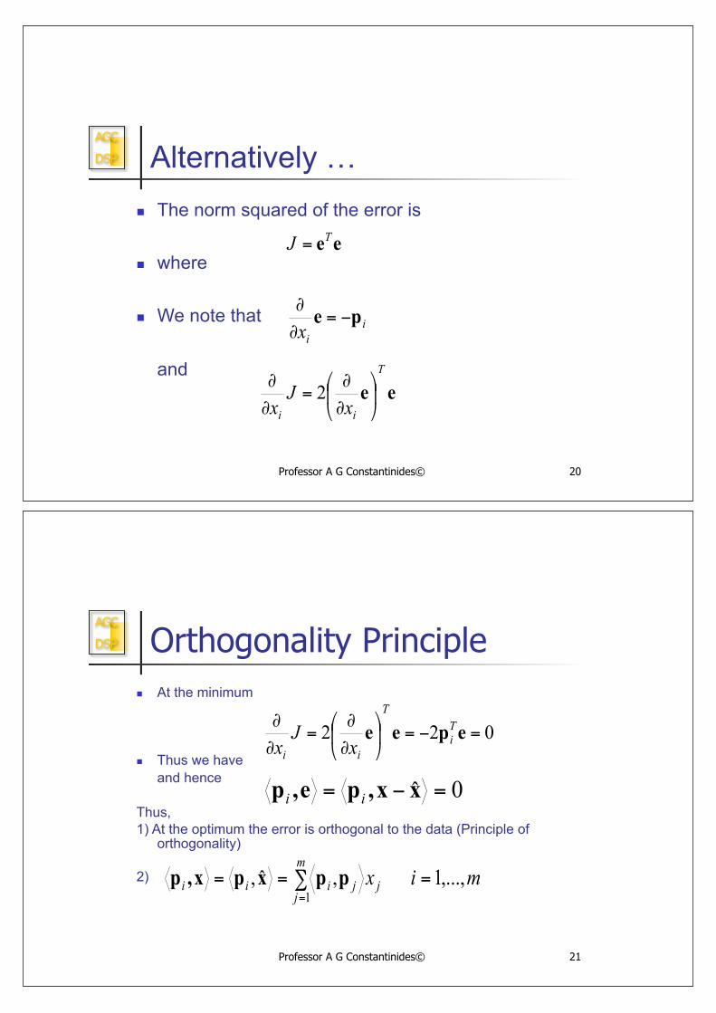
Alternatively …
!! The norm squared of the error is
!! where
!! We note that
and
AGC
DSP
Professor A G Constantinides© 21
Orthogonality Principle
!! At the minimum
!! Thus we have
and hence
Thus,
1) At the optimum the error is orthogonal to the data (Principle of orthogonality)
2)

AGC
DSP
Professor A G Constantinides© 22
Orthogonality Principle
!! Thus for
Hence or
AGC
DSP
Professor A G Constantinides© 23
Orthogonalisation
!! A signal may be projected into any linear space.
!! The computation of its coefficients in the various
vectors of the selected space is easier when the
vectors in the space are orthogonal in that they are
then non-interacting, ie the evaluation of one such
coefficient will not influence the others
!! The error norm is easier to compute
!! Thus it makes sense to use an orthogonal set of
vectors in the space into which we are to project a signal

AGC
DSP
Professor A G Constantinides© 24
Orthogonalisation
"! Given any set of linearly independent vectors that span a certain space, there is another set of independent vectors of the same cardinality, pair-wise orthogonal, that spans the same space
"! We can think of the given set as a linear combination of orthogonal vectors
"! Hence because of independence, the orthogonal vectors is a linear combination of the given vectors
"! This is the basic idea behind the Gram-Schmidt
procedure
AGC
DSP
Professor A G Constantinides© 25
Gram-Schmidt Orthogonalisation
!! The problem: (we consider finite dimensional spaces
only)
!! Given a set of linearly independent vectors
to determine a set of vectors that are pair-
wise orthogonal
!! Write the ith vector as
AGC
DSP
Professor A G Constantinides© 26
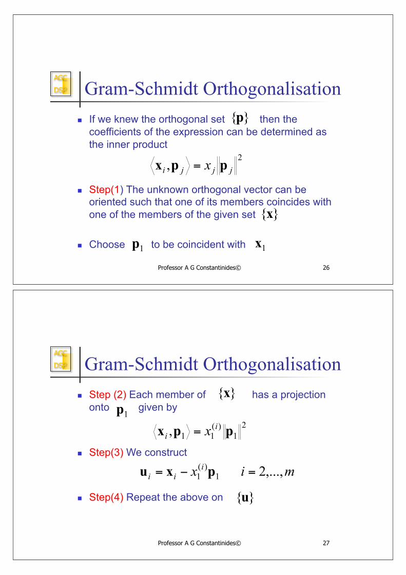
Gram-Schmidt Orthogonalisation
!! If we knew the orthogonal set then the
coefficients of the expression can be determined as
the inner product
!! Step(1) The unknown orthogonal vector can be
oriented such that one of its members coincides with
one of the members of the given set
!! Choose to be coincident with
AGC
DSP
Professor A G Constantinides© 27
Gram-Schmidt Orthogonalisation
!! Step (2) Each member of has a projection
onto given by
!! Step(3) We construct
!! Step(4) Repeat the above on

AGC
DSP
Professor A G Constantinides© 28
Gram-Schmidt Orthogonalisation
!! Example: Let
!! Then
!! And the projection of onto is
AGC
DSP
Professor A G Constantinides© 29
Gram-Schmidt Orthogonalisation
"! Form
!! Then

AGC
DSP
Professor A G Constantinides© 30
Gram-Schmidt
-2 -1.5 -1 -0.5 0 0.5 1 0 0.1 0.2 0.3 0.4 0.5 0.6 0.7 0.8 0.9 1
Projection of in
AGC
DSP
Professor A G Constantinides© 31
3-D G-S Orthogonalisation
-1 -0.5
0 0.5
1
-1 -0.5
0 0.5
1 -1
-0.5
0
0.5
1

AGC
DSP
Professor A G Constantinides© 32
Gram-Schmidt Orthogonalisation
!! Note that in the previous 4 steps we have
considerable freedom at Step 1 to choose any vector not necessarily coincident with one
from the given set of data vectors.
!! This enables us to avoid certain numerical ill-
conditioning problems that may arise in the Gram-Schmidt case.
!! Can you suggest when we are likely to have ill-conditioning in the G-S procedure?


![Tensor DecomposiTions - Imperialmandic/Tensors_IEEE_SPM_March_2015.pdf · [From two-way to multiway component analysis] Tensor DecomposiTions for Signal ... interest in tensors in](https://img.pdfslide.us/doc/110x75/5b84e27b7f8b9aef498d3bde/tensor-decompositions-mandictensorsieeespmmarch2015pdf-from-two-way.jpg)