LA-12235-MSCIC-14 REPORT COLLECTION

p.-..

r

r—--_—

REPRODUCTION -COPY

r.

DSD Technology:

A Detonation Reactive Huygens Code

Los AkmimsLos Alamos National Laboratory is operated by the University ofCalifornia forthe United States Department of Energyunder contract W-7405-ENG-36.

-.

,,,,,,,,,,,,,,,,,,,, ,,,,,,,,,,,,,,,,

,,,,,,,,,,,,

,,,,,,,,,,,,

ANAffiwdiw Actio@psl OpportunityE@oycr

This nywt was prrparrd as an ncrmmt of uwkspmsordhyma~.?ncyIJhUnited%sk Gorwwncsnl. FJeithcv‘7%rRegents of the Unizwsit~ o/ California,th~’UnitedStat.-sGomvwncnt nor any nxcny thmof, nor any OJthezrwsployccs, mikes [mywarranty, cxprw or implid, or uwnws ursv legal liability or responsibility for tlwaccurm>y,compktencss,or uscftdrwssofmry injmratik, appwutns, product, or proms disclosed, orrrpn’srnls thdits usc r(~ou/dnot infrin<feprivate/y ozmk’drights. R@wwc herrin to mIy spwijiconmtercial product, proms, or service frytrade name, hmienurrk,nwtufflctuwr, w 0Mcri(Ji5t,d~jnot necessr?ri$corsstituk’or imply its endorsement, r~sco)~t)rle~ltitio~r,or fmwing by The Re$enis0/the Uniwrstty of California, the United .9ak Gowrmncnt, or any ogtwy ther+. The weuwand opinious of authors ~xprcssedherein do not necessarily state or re)kt those of The k“<@’}Jh o~the University o/ Calfor/lia, theUnited States Gozwnnwnt, or mty qywy thweo~,

●.!

Eii==l‘L .-l

I

k--k-F=

LA-22235-MS

UC-741and UC-705Issued: ]uly 1992

DSD Technology:

A Detonation Reactive Huygens Code

JohnBdzilWildon Ficketi

——

Los Akauiiilm

.

Los Alamos National LaboratoryLos Alamos,New Mexico 87545

9,,

I.

II.

III.

N.

v.

w.

VII.

CONTENTS

INTRODUCTION . . . . . . .,. .,. OO. OOO

GEOMETRY AND NOTATION . . . . . . . . . . . .

EQUATIONS . . . . .

INPUT AND OUTPUT

SAMPLE PROBLEMS

EXACT SOLUTIONS .

CODE STRUCTURE .

REFERENCES . . . .

Appendix A. SCALING

. . . . . ..OOO . ..O. .

. . . . . ..oee . . ..O .

.00. . . ..OO ..OO.

. . . . . . . ..O ● e...

. ...0 . . . . . ..eoe

. . . . . . . . . . .OO*O

. ..00 . . . . . .OO, O

Appendix B. DETONATION FAILURE MODELS . . .

1

3

6

9

18

33

38

42

43

44

v

DSD TECHNOLOGY:

A DETONATION REACTIVE HUYGENS CODE

by

John Bdzil and Wildon Fickett

ABSTRACT

The length of the reaction zone strongly influences the speed ofpropagation of detonation in multi-dimensional explosive pieces.Detonation Shock Dynamics (DSD) properly accounts for these effectsin detonation wave-spreading problems when the radius of curvatureof the multi-dimensional detonation shock is large compared to theexplosive’s reaction-zone length. This report is a user manual forour two-dimensional implementation of this method; a FORTRANsubroutine called DSD Technology.

I. INTRODUCTION

Modeling detonation propagation in complex shaped explosive pieces is an importantproblem in the design process for explosively powered devices. The computationalproblems that arise are difficult, because the physics import ant to the problem occurson many disparate length scales. For example, the device size is typically many ordersof magnitude larger than the size of the explosive’s detonation reaction zone. One ofthe principal shortcomings of the computer models that are presently used for multi-dimensional explosive engineering design is their inadequate treatment of the explosive’sdetonation reaction zone. Current uniform-grid methods lack the resolution to calculateboth the broad gas expansion region and simultaneously the thin reaction zone withreasonable detail. Consequent ly, detailed calculations that resolve the reaction zone areseldom performed. Typically, the reaction zone is assumed to be inihitesimally thin and itsdynamics is modeled by a scale independent detonation Huygens construction. This modelassumes that detonation propagation is purely a geometric problem; the multi-dimensionaldetonation wave is a shock that expands normal to itself at the constant Chapman-Jouguetdetonation speed, DCJ. When the detonation reaction zone is exceedingly short comparedto a representative dimension of the explosive piece, this simple model yields good results.

In recent years, concerns about accidental initiation of detonation have led to the use ofinsensitive explosives; explosives with reaction zones orders of magnitude longer. Because

1

of the increased length of their reaction zones, the detonation speed departs significantlyfrom .DCJ. For example, for these explosives the detonation speed is slower for expandingwaves than for plane ones, and near edges the detonation speed can be significantlyreduced; this reduction causes the detonation wave to become curved. Drawing on recenttheoretical research on multi-dimensional detonation, we have developed a theory calledDSD that incorporates the explosive’s scale dependency; this theory allows us to modelfinite reaction zone effects. DSD is the acronym for the “Detonation Shock Dynamics”theoryl’2 developed by John Bdzil and Scott Stewart. This theory provides a recipe forpropagating a detonation wave front without calculating the flow behind it. A central resultof the theory is that the normal velocity D of the wave front at any point depends onlyon the wave curvature K at that point. This has the effect of reducing the dimensionalit yof the det onat ion propagation problem by one. Thus a problem with either a plane oraxis of symmetry (a two-dimensional p,roblem) becomes a one-dimensional problem. Afunction D(K) characterizes each explosive and is considered to be a material property.This function can be calculated theoretically if the equation of state and reaction rates areknown but is obtained in practice from simple calibration experiments.

DSD is a low-frequency (long transverse wavelength) asymptotic theory. Thegoverning equation is a parabolic partial-differential equation (PDE), similar in form toBurgers’ equation (see Ref. 3, ch. 4), but with a complicated coefficient involving integralsover the solution. For the theory to apply, the radius of curvature of the front must bemuch larger than the length of the reaction zone.

The theory is analogous to Whitham’s “Geometrical Shock Dynamics” theory, Ref.i3, ch. 8), but applies to detonation waves instead of inert shocks. The mathematical orm

of “Geometrical Shock Dynamics” (a hyperbolic theory) is different from DSD (a parabolictheory . This difference in form follows from the fact that inert shocks decelerate as they

iexpan whereas det onat ions accelerate.

As D(K) drops below DCJ, the thermodynamic state point from which the explosiveproducts undergo expansion changes. The Chapman-Jouguet state is not the properstarting state. Given D(K) and a compatible equation of state for the products, theproper starting state for the numerical computation of the products region (the workingfluid) can be calculated. Since D typically varies along the shock, the starting state forthe explosive products is different at the center and edge of the explosive piece. Thus byincorporating the reaction zone effects into the detonation propagation model, DSD alsoyields the proper starting point for the expansion of each parcel of explosive product.

Brian Lambourn and Damian Swift4 at the Atomic Weapons Establishment (AWE)in England have developed a theory similar to DSD. They call their implementation of thetheory the Whitham-Bdzil-Lambourn (WBL) detonation model.

The plan of this report is as follows. The problem geometry and intrinsic coordinaterepresentation that we use are presented in Chap. II. The evolution equation for the shock,the boundary conditions and D(K) functions are discussed in Chap. III. In Chap. IV wedescribe the structure of the input deck that is used to set up problems. Selected outputfrom seven sample problems is presented and discussed in Chap. V. Chapter VI is a brieftutorial on the DSD method. The structure of the code is described in Chap. VII. Thescaled variables used in the code are described in Ap endix A. The detonation failure

fmodels currently implemented in the code are describe in Appendix B.

2

11. GEOMETRY AND NOTATION

The detonation is assumed to have the usual Zeldovich-von Neumann-Doering (ZND)structure, that is, a shock followed by a reaction zone. The theory tracks the leading shock,which we will refer to as the shock— .

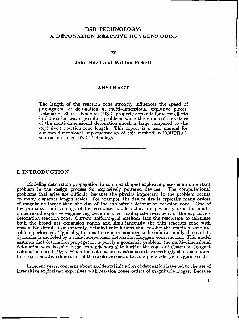
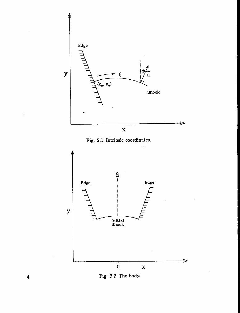
The governing equations are written in the intrinsic coordinates shown in Fig. 2.1.This is a key step in constructing a tractable and transparent theory. The independentvariables are ~, the dist ante (arclengt h) along the shock, and the time t. The dependentvariable is ~, the ~ of the shock, defined as the angle between the vertical and theout ward (i. e., drawn in the direction of propagat ion) normal to the shock, with # positivefor clockwise rotation of the normal from the vertical.

The laboratory coordinates x and y of the shock (cartesian coordinates in the framewith the undisturbed explosive at rest) at a given time t are related to the intrinsiccoordinates ~ and # by

(2.la)

Y(() t) = ‘Ye(t) -J<sin 4((’, t)de . (2.lb)

The integration begins at an edge point z.(t), ye(t) where ~ is assigned the value zero.

We use the term body to denote the piece of explosive in which the wave propagates.For our purposes we regard the body as bounded by a specified initial shock and two edges,as shown in Fig. 2.2. The edges are the two physical edges of the explosive between whichthe shock propagates.

We treat only the (mathematically) “one-dimensional” case, that is, with one spaceand one time variable. There are two possible symmetries which we refer to by the names~ and cvlinder. These are defined as follows:

. (1)

(2)

Slab

Fig. 2.2 is a cross section of a body of infinite extent in the direction normal to thepaper; all curves (edges and shock) are cylindrical surfaces with generators normal tothe paper.

Cylinder

Fig. 2.2 is a cross section of a figure of revolution about the centerline x = O.

For either of these geometries, the terms we use to describe the shape of the shock oran edge will refer to the section in the plane of the paper. Thus, for example, a shock

3

Edge

●

Shock

x

Fig. 2.1 Intrinsic coordinates.

EEdge Edge

o x

Fig. 2.2 The body.

Y

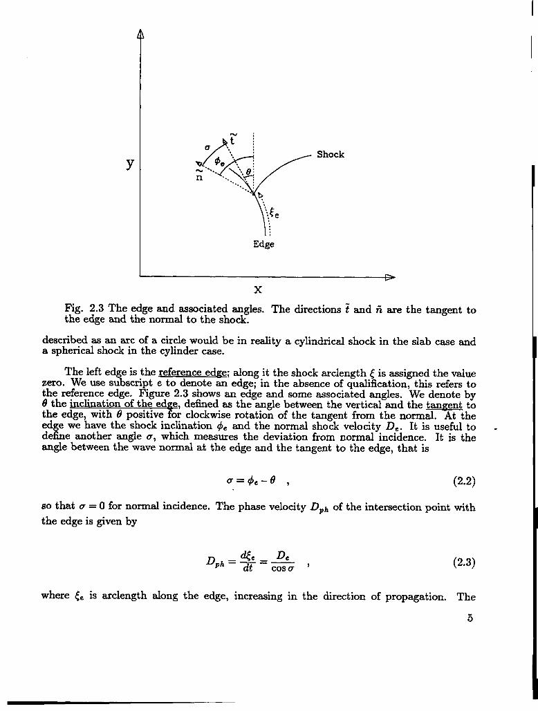
Fig. 2.3 Thethe edge and

Shock

1:Edge

x

edge and associated angles. The directions ? and ii are the tangent tothe normal to the shock.

described as an arc of a circle would be in reality a cylindrical shock in the slab case anda spherical shock in the cylinder case.

The left edge is the reference edge; along it the shock arclength f is assigned the valuezero. We use subscript e to denote an edge; in the absence of qualification, this refers tothe reference edge. Figure 2.3 shows an edge and some associated angles. We denote by6 the inclination of the edge, defined as the angle between the vertical and the tarment tothe edge, with @ positive for clockwise rotation of the tangent from the normal. At theedge we have the shock inclination q$~and the normal shock velocity De. It is useful to .define another angle a, which measures the deviation from normal incidence. It is theangle between the wave normal at the edge and the tangent to the edge, that is

so that a = O for normal incidence. The phase velocity Dph of the intersection point with

the edge is given by

(2.3)

where C= is arclength along the edge, increasing in the direction of propagation. The

5

solution of Eq.552.3), e(t) and the prescribed edge shape, tl(~e) combine to yield the edge

~coordinates z, (t , ye (t

111(

(1)

Xc(t) = (2.4a)ze(0) + Jte sin ~(t~)d~~ ,

ye(~)= y.(o)+ Jt= COSO(~)d~J . (2.4b)

EQUATIONS

~uations of Motion

The governing equations for ~(~, t) are

$,+ B+( = -De = -D’(/c)(#<< + kSt) (3.la)

J(

BZ Dt$ed[ + D, tanc (3.lb)o

K=$l++s (3.lC)

S E sin ~/x (3.ld)k = 0/1 for slab/cylinder symmetry . (3.le)

The shock kinematics is described by Eq. (3.la), which resembles Burgers’ equation

Ut+ Uuz = vu== , (3.2)

with the coefficient lil the propagation speed and –D’( K) s –dD( ~)/d~ the “viscosity” v.The first (integral) term in B represents the change in shock surface from wave spreading,and the second term the change from the intersection at the edge (note that the secondterm is zero for normal incidence). For slab symmetry, the curvature K is just the reciprocalof the local radius of curvature of the shock.

The function D(K) characterizes the explosive dynamics and must be specified bythe user. Typically, it is determined by experiments in a standard geometry, themost common being the so-called “diameter-effect” experiment, which measures steadydetonation velocity as a function of charge diameter in a “rate stick”-a long cylinder ofexplosive. The determination of D(K) from these data is discussed in Ref. 5. We consideronly -D’(K) >0.

6

The governing equations above are writ ten in scaled variables; see Appendix A.~In these variables, the Chapman-Jouguet (CJ) detonation velocity is unity, and the CJreaction time is unity or at least O(l).

For computation, the integral term in the coefficient 1? is split into two parts. Wewrite it as

(3.3)

This has the advantage that the integral, which must be done numerically, is a small term,because (D – 1) is the deviation of the (scaled) wave velocity from the

Another form of these equations is useful both for computationdefine a new angle variable u

u=~-e ,

CJ value of unity.”

and analysis. We

(3.4)

which has the nice property that u = O at an edge to which the wave is normal. In thisvariable the governing equation is

ut + But = -D’(/c)(uct + kSC) - 8’(t) . (3.5)

The added source term 0’ is ~he time derivative of the left edge angle 0 at the point atwhich the shock intersects the edge.

(2) Boundary Conditions

For a free edge (vacuum) we ask whether the flow is supersonic or subsonic in theframe attached to the moving intersection point of the shock and the edge, i.e., whether

the quantity (l ~ 12–Cz) at the shock, where ~ is the vector particle velocity in this frameand C is the sound speed, is greater than or less than zero. If the flow is supersonic, signalsfrom the edge do not enter the explosive, and we apply no boundary condition. If the flowis subsonic, we force it to be sonic by setting the edge angle rY to the critical value, thevalue for which the flow is sonic. In effect, overall we bound a from below by the criticalvalue, a=. For the polytropic fluid equation-of-state (EOS) with finite, single-step reactionrate, the critical value of u is given by

(3.6)

For instantaneous reaction (a Huygens wave), the critical value is a = O.

7

In general, the total arclength & of the shock between the two edges is changing with~time. For our numerical method we need this total arclength along the shock and its rateof change with time. This derivative is given by

(3.7)

where the subscript 2 denotes values at the right edge.

(3) mans verse Acoust ic wave SDeed

It is of some interest to know how fast an acoustic signal, for example, the head of anedge rarefact ion, propagates into the explosive along the shock. The speed of a transverscwave along the shock is given by

(3.8)

where (W is the location of the wave head, +/- denotes a rarefaction originating at theleft/right edge, C is the sounds eed and U is the component of the particle velocity normal

{to the shock in the shock attac ed frame. The right-hand side (RHS) is evaluated on theexplosive shock. For the polytropic fluid EOS, the first term is

(3.9)

The high frequencies associated with the acoustic wave head are not strictlycompatible with a low-frequency theory like DSD. This is particularly an issue at earlytimes. Consequently, there is some ambiguity associated with identifyin a proper origin

!for the acoustic source, ~Wo. Generally, select ~Woto be a short distance in rom the physicaledge. This protects the acoustic source from early-time, high-curvature DSD transients.

(4) D(K) Functions

Qualitative changes in the shock propagation can occur for different D(K) that satisfy-D’(K) z O. When D = 1 – LYK with Q = constant for all 0< K < m, then the shock passesover every point in the explosive. We use this simple model for the sample problems.. . . -. --described in Chap. V.

Detonation in real explosives cannot be sustained in regions

where Kf, the curvature at which detonation fails, is different for

where K > nf and

different explosives.

8

For example, not all the explosive detonates in the vicinity of a sharp corner. Near suchfeatures, the detonation shock does not extend into the corner but terminates at an interiorpoint defined by K = Kf. The locus of all such points defines a virtual edge (interior to

the physical edge). The explosive between the physical edge and the virtual edge fails todetonate; it does not undergo significant reaction on a relevant time scale. An example ofa D(K) function that can m-odel-this behavior is

D = Df + (1 – Df)~m

where K ~ K~ and the failure velocity, D ~, satisfies O < Df <

with these properties is described in Appendix B.

IV. INPUT AND OUTPUT

(1)

A sample input file is

‘run’‘fluid’‘Dkap’‘geout

l=VP1‘@!3er’‘xnet’‘tnet’‘it’‘bcl’‘bcr’

‘Onion’3.0 0.01 0.11.01 -1.0 0.0 -1.573 0.0 1.0 0.00.0 128 8.01.0 4 3.752 -1.57 1.0 +1.031

7 (3.10)

1. A detonation failure model

!alpha = 0.1

! gonic

!no bc‘bcrt’ 2 ! soft right‘tvav’ 1 0.125 !twave (left bndry)‘ref 1’ 5 0.1 !Cyl . w/ linear D-kappa‘dials’ 1.0 0.001 0.001

The general structure of the input line is keyword, option flag, data.

The run line is special. Not all lines have the option flag. For example, in the secondline, fluid is the keyword; there is no option flag, and 3.0 and 0.0 are data items. In thethird line, Dkap is the keyword; 1 is the option flag; and 0.1 is a data item. An exclamationmark designates the rest of the line as a comment. A line with an exclamation mark incolumn one is a comment line.

The only restriction on the order of the lines is that the run line must be present andmust be the first line. Its string (Onion in the example) appears in headings on the output.The remaining lines can appear in any order; only those required for the problem at handneed be present.

9

10

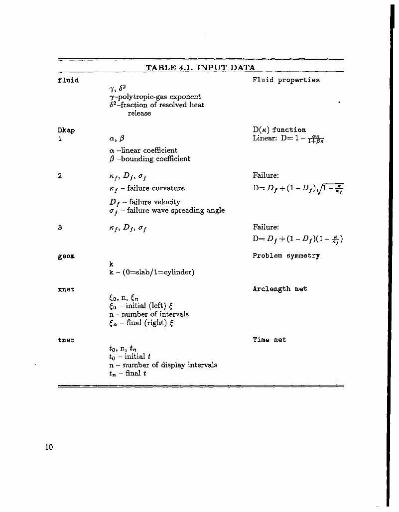
TABLE 4.1. INPUT DATA

fluid Fluid properties‘y, 62

7–pOlytrOpic-ga exponentt$z-fraction of resolved heat

4

release

Dkap1 cl!,@

2

3

geom

xnet

tnet

CY–linear coefficient/3-bounding coefficient

~f, Df, ofKf - failure curvature

Df - failure velocitya f – failure wave spreading angle

kk – (O=slab/l=cylinder)

to, n, tnco - initial (left) ~n - number of intervals~n - final (right) ~

D(Ic) functionLinear: D= 1 – ~

Failure:

D= Df+(l-llf)(l-~)

Problem symmetry

Arclength net

Time netto, n, tn

to – initial in- number of &play intervalstn - final t

TABLE 4.1. INPUT DATA (continued)

ic Initial Condition

1 fP Line

~ - angle

2 ~, r, s Circle

# - initial angler – radiuss – sign (q$~)

3

edgel, edger1

#, r, s, fle dp10 Data file

dp10 - contains (, d, #It

Edge

x> Y767 tern Line

X,y - initial point6 – angle~ern- edge arclength

maximum

& Y7 67ry % tern Circle

r – radiuss – sign of d8/d&

x> Y, e, (em, fles dp8/dp9 Data iile

dp8/dp9 – contain list of(e and 6. for(left/right) edge

bcl, bcr Boundary conditions

1 No b.c.

2 “o Fixed angle ci

CT– angle

3 ~cj Letl> Cet2~ g Sonic, <e ~ ~e~l

o= - critical sonic angle NO b.c., ~et2 s (e < fetl

(eti - edge arclength at Fixed angle cr,

b.c. transition points (e< ~efz

11

.

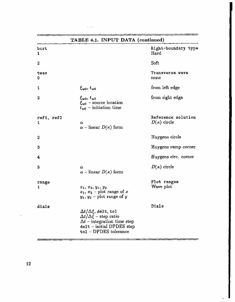
TABLE 4.1. INPUT DATA (continued)

bcrti

2

twavo

1

2

ref 1, ref21

2

3

4

5

range1

dials

Right-boundary typeHard

soft

Transverse wavenone

two, two from left edge

two, two from right edge

CWo- source locationtWO– initiation time

Reference solutionc1 D(K) circlea – linear D(K) form

Huygens circle

I-Iuygens ramp corner

Huygens circ. corner

D(K) circle

Plot rangesWave plot

Q’a – linear D(K) form

Zl, Z2, ~1, yzzl, zz – plot range of x

Y1, Y2 – plot range of y

DialsAt/A~, delt, tolAt/A~ - step ratioAt - integration time stepdelt - initial DPDES stept ol – DPDES tolerance

12

v

The input data specifications are summarized in Table 4.1. Detailed specifications for eachline follow.

RUN- Run Label

The run label is the second string on the line. It appears in the output headings.

FLUID – Fluid Parameters

‘)f,&;2= polytropic-gas exponent

= fraction of resolvedenergy release

The fluid equation-of-state is used in two places. It is used in calculating the sonic characterof the flow at the edge in the sonic boundary condition, option 3 under bcl, bcr. It isalso used in the separate calculation of the (transverse) speed of the head of the edgerarefact ion wave along the shocks under t wav.

The parameter 62 applies to the SRHR model (see Ref. 6). For this model, the sonicboundary condition depends on 82 and ~.

DKAP – D(K) Relation

1 a, /9 Lineara, @ – coefficients in

D = 1 -aK/(1 +PK)

The D(K) relation is linear, with coefficient a for [Kl small, and D(K) approaches 1 – a//3for K large.

2 ~f> Df> ~j . Failure Model Aaf – spreading angleDj, tcf – coefficients in

D = Df + (1 - Df)+ – tcf~f

For Model A, detonation propagates onlyin regions Where K < ~f. The detonation fails

at~= ~f, with D’( ~f ) -+ W. The spreading angle, af of the failure wave ~ong the ShOCkis measured relative to the shock normal. See Appendix B for details.

3 ~f~ Df> of Failure Model BDf, ~f – coefficients in

D =Df +(l-Df)(L~/tcf)

Model B is similar to Model A above except that D(K) is linear and ~’(~f) = -(1 -Df )/~f.

13

.

14

Y

v“Edge

s< vo S>o

x

Fig. 4.1 Sign ofs for the circular-arc edge (s= d@/d&) and initial shock (s = d#/d&).

Y O8(>0 (9(<0

Shock Shock

>

x

Fig. 4.2 Edges – circles

left: e=eO–: left:

right: tl=e~+$ right:

GEOM– System Symmetry

kk- ((1 = slab /1 = cylinder)

For slab symmetry, the body is infinite in extent in the direction normal to the paper.For cylinder symmetry, the body is a figure of revolution about the x = O centerline.

IC – Initial Condition

1 4 Line$- angle

The initial shock is a straight line, which has inclination ~ at the left edge.

2 +, r, s Circle~ - angler – radiuss – sign of @t

See Fig. 4.1. The initial shock is an arc of a circle of radius r and has inclination ~ at theleft edge. The parameter s (+1.0) gives the sign of the curvature.

3 ~, r, s Data File

The input file is dp10. Its fist three lines contain four data fields each. Of these, all butthe first field in the first line (which contains the # points in the initial data) are dummynumeric fields. Lines 4 thru (3 + # points) contain the triplets (~, ~, ~<) that describethe initial shock shape. The file dp10 is written by the code at the final output time. Itis used as initial data to solve problems with complex boundaries as a sequence of simplerproblems.

# points xx xx xxxx xx xx xxxx Xxxxxx

t 4 46

EDGEL, EDGER- Left, Right Edge

Line

9- angle&m - edge arclength

maximum

The edge is a straight line at angle O through (x,y), the intersection of the edge with theinitial shock.

2 x> YY$Yry % tern Circler – radiuss – sign of d#/d~e

15

See Fig. 4.2. The edge is a circular arc of radius r, total edge arclength &~, initial angle 6,~through (x,y), the point of intersection of the edge with the initial shock. The parameters (+1.0) gives the sign of the curvature. A default value of & is used when no value (i.e.,zero) is e-ntered. -

3 xf Yt 6Y[em~e, 6.(C - edge arclengtht9. – angle of

edge tangent

The input file is dp8/dp9 for the left/right

# points

Ce, 0.

Data File

edge. Its format is

BCL, BCR – Left, Right Boundary Condition (b.c.)

1 No b.c.

No boundary condition is to be applied. This is used at a supersonic edge.

2 c Fixed angle aa – angle

The intersection angle a between the shock’s normal and edge tangent is to be fixed at thegiven value.

3 ~cy Cetlj~et29o sonic,& ~ (etlaC – critical sonic angle NO b.c., ~ctz s C. c cetl

&eti- edge arclength at Fixed angle a,b.c. transition points & < &t2

The condition to be applied when fe z ~.tl is

If ~cr > a., no b.c. (supersonic)If* fY<ac, o=clc= constant (subsonic),

where ac >0 is the angle at which the flow at the edge is sonic, the (-) sign applies at theleft boundary and the (+) sign at the right. If the flow at the edge issonicor subsonic,make it sonic. No boundary condition is applied when &t2 < & < ~etl. When & < &t2, the

16

.

intersection angle bet ween the shock’s normal and edge tangent is fixed at a. The defaultvalue for aC is the polytropic gas expression,

ra. = arctan g .

4 Huygens, ~. z ~etlNO b.c., <etz s <e < ~etlFixed angle a,

(~ < ~et2

This is the prescription for the Huygen’s solution, which is normal incidence. The algorithmis that desribed in 3 above, with UC= O.

BCRT– Right Boundary Type

1 Hard2 soft

The “hard” right boundary applies the given right boundary condition (from the bcr line)at the right edge, lengthening or shortening the comput ation’s ~-length as required. Forthe “soft” right boundary the computational {-length is fixed; its right end does not ingeneral coincide with the right edge, See Chap, VII in this report.

TWAV– ‘lh.nsverse Wave Flag

This option tracks the head of an acoustic wave along the DSD generated shock. The sourceof the disturbance is an edge rarefact ion. For early times the head oft his acoustic wave canlag the DSD calculation o~the disturbed shock. This is becausetheory.

o1 two, two2 two, two

two - source locationtwo – initiation time

Note: do not start the wave precisely at the

“ REF1, REF2 – Wference Solutions

edge.

DSD is a long-wavelength

No waveLeft-edge waveRight-edge wave

The reference solutions are displayed on the wave plot for comparison with the calculation;that specified by ref 1 (linear D(K)) with a dashed line, and that specified by ref 2(Huygens) with a chain line.

lor5 a D(K) circlea – from linear D(K)

2, 3, 4 Huygens D = 1 circle

17

The reference solution refl is the exact solution for an expanding circular wave withD = 1 – QK (see Chap, VI). The solution ref 2 is a Huygens wave.

DIALS - Integration Control

Equations (2.3), (3.la), (3.lb), (3.7) and (3.8) control the evolution of the shock. TheInternational Mathematical Software Library (IMSL) method of lines subroutine DPDESis used to integrate Eq. (3. la). Equation (2.3) is integrated with a centered-differencescheme, while Eqs. (3.7) and (3.8) are integrated with a forward-difference scheme. Thexnet line gives the initial mesh spacing along the shock (At = (~~ – to )/n). The time step,At is entered indirectly through At/Af. Delt k the initial DPDES time step and t ol isthe DPDES error tolerance.

2“Q@@

Terminal output is designed to monitor the progress of the calculations. A line isprinted after each calculation step. Here kt is the number of the step, and nxr is thenumber of mesh points between the edges. For each edge the sonic character son (0/1for sub/super), the boundary condition type bdry (1/2/3 for no b.c./fixed a/K= ICj), the

detonation state fail (1/2 for detonating/failing) and the angle CTare shown. If the timeis a display time, the letter “d” appears after the time. If this step involved a new DPDESstart, the let ter “n” appears after the value of nxr. The current DPDES time step dphand the total shock arclength xi2 I are also shown.

The printed output at each display time consists of one line containing the loop indexkt, the time t, and edge quantities, and then the mesh print, consisting of one line for each

mesh point, containing c, d, 4;, D, B, z, y, and x and y for each reference solution. Thisoutput is written to file do. In addition, the z, y coordinates of the wavefront are writtento dpl and the ~, @ coordinates of the fronts are written to dp5.

The graphical output at the end consists of four plots: (1) the Fronts, showing thebody, any failure Ioci, and successive shock shapes, (2) the wave angle ~ vs. arclemzth ~,(3) the Phase Velocity D vs. time at the ends of the shock, and (4) the coefficient

Vs. arclen~th ~. Plots 1, 2, and 4 show one curve for each display time.

V. SAMPLE PROBLEMS

We give the input data and results for several sample problems. The input files aregiven in Table 5.2. The output represents a selection; the complete output is not given foreach problem. Data decks for a wide variety of sample problems are included at the endof the code. Instructions for running them can be found in Chap. VII of this report.

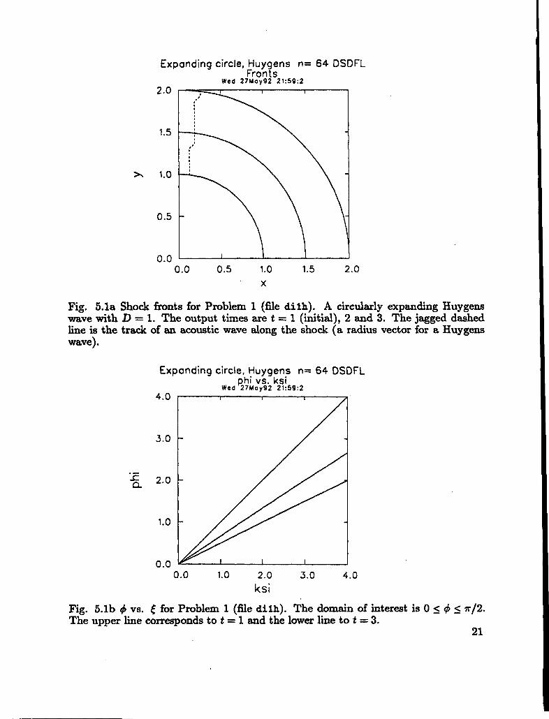
Problem 1 (data file di Ih and Figures 5.1) is the Huygens solution for an expandingcircle. The shock shapes at three times are shown in Fig. 5.la. The left edge is a vertical

18

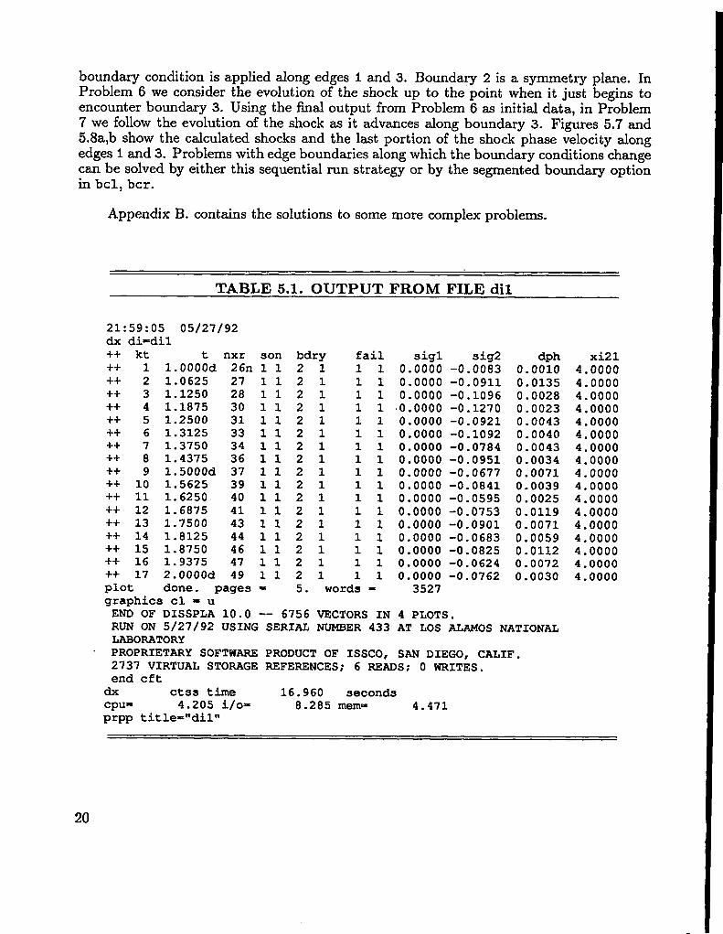
straight line, the right edge is a horizontal straight line, and the initial shock is a circle ofunit radus. As specified by the ‘Dkap’ line of the input, linear II(K) with a = Ogives D = 1for the Huygens’ solution. The left b.c. is that the wave be normal to the edge (the flowwill always be sonic in this problem). The right boundary is a soft boundary, i.e., the rightedge is the terminal locus for the display. The computation arclength remains ilxed at itsinitial value of 4 (’xnet’ line). Initially, the end point ~~ = 4 of the computation arc lieswell beyond the right edge (which is at ~ = 1 x (7r/2) at the initial time t = 1). TO have thecomputation arc extend to the right edge up to time 4, we would have set & >4 x (z/2)(with a corresponding increase in computation time). The jagged line originating at theleft boundary in Fig. 5.la is the track of the acoustic wave head along the shock. It marksthe leading edge along the shock of the rarefaction advancing from the left boundary. Theroughness of the track gives a measure of the calculat ional mesh size. A total of 64 meshpoints span the shock from & = O to ~ = 4 x (7r/2). The angle # vs. & for three times isshown in Fig. 5.lb. Table 5.1 shows the output written to the screen by this run.

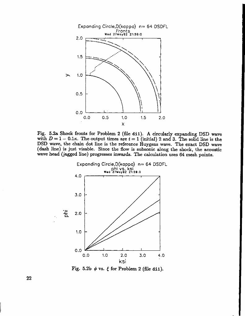
Problem 2 (data file dil and Figures 5.2) is the expanding circle for D = 1 – aK,a = 0.1. The geometry is the same as Problem 1. The left b.c. is a = O (normal incidence).The right b.c. is a soft boundary identical to the right boundary in Problem 1. The tworeference solutions appear on the wave. plot for comparison: (1) Huygens solution (chaindot line) Wd (2) exact solution (dashed line) (see Chap. VI of this report). The totalnumber of mesh points is 64.

Problem 3 (data file dilp and Figures 5.3) is identical to Problem 2 with the exceptionthat the number of mesh points is increased to 128. Comparing the results of theseproblems gives a measure of the sensitivityy of our numerical algorithm to mesh size. Thedependence on mesh size is weak. Also shown are the Huygens solution (chain dot line)and exact solution (dashed line).

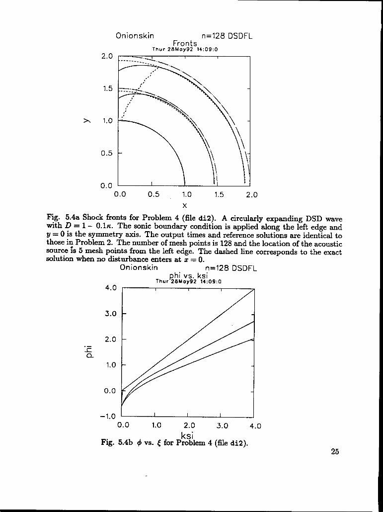
Problem 4 (data file di2 and Figures 5.4) is similar to Problem 2 except that the sonicboundary condition is enforced along the left edge. It is a simple model of the onionskinexperiment with the symmetry axis along y = O. Note that along the left edge, the shocksshown in Fig. 5.4a curl back. The sonic boundary condition provides a model for anunconfined edge. A plot of the phase velocities in Figure 5.4c shows the velocity along theleft edge (lower curve) is well below the velocity along the right edge (upper curve).

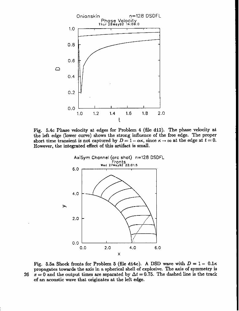
Problem 5 (data file di4c and Figures 5.5) considers a detonation with D = 1 – a~,~ = 0.1 propagating in a c~ed channel (WC shot). The geometry is cylindrical (k = 1),

with x = Othe axis of symmetry. The sonic boundary condition is applied along both edges.Figure 5.5b shows that the total shock arclength increases with time. As the right edgeadvances along the shock, Fig. 5.5c shows that the phase velocity increases there. Althoughthe flow is originally sonic along this edge, after t = 3.5 the flow becomes supersonic. Theleft edge pulls away from the shock. This leads to a phase velocity near 0,85 along thisedge until late time when the convergence toward the symmetry axis accelerates the wave.

In problems 6 and 7 we consider an initially circular detonation propagating in anexplosive whose geometry is shown in Fig. 5.6. These two problems (data files di6cbl,dp9 and di6cb2 and Figures 5.7-5.8) are designed to be solved sequentially. The sonic

19

boundary condition is applied along edges I and 3. Boundary 2 is a symmetry plane. InProblem 6 we consider the evolution of the shock up to the point when it just begins toencounter boundary 3. Using the final output from Problem 6 as initial data, in Problem7 we follow the evolution of the shock as it advances along boundary 3. Figures 5.7 and5.8a,b show the calculated shocks and the last portion of the shock phase velocity alongedges I and 3. Problems with edge boundaries along which the boundary conditions changecan be solved by either this sequential run strategy or by the segmented boundary optionin bcl, bcr.

Appendix B. contains the solutions to some more complex problems.

TABLE 5.1. OUTPUT FROM FILE dil

21:59:05 05/27/92dx di=dil++ kt t nxr son bdry++ 1 1.0000d 26n 1 1 2 1++ 2 1.0625 271121++ 3 1.1250 281121++ 4 1.1875 301121++ 5 1.2500 31 11 2 1++ 6 1.3125 33 11 2 1++ 7 1.3750 341121++ 8 1.4375 361121++ 9 1.5000d 37 1 1 2 1++ 10 1.5625 39 11 2 1++ 11 1.6250 40 11 2 1++ 12 1.6875 41 11 2 1++ 13 1.7500 43 11 2 1++ 14 1.8125 44 11 2 1++ 15 1.8750 461121++ 16 1.9375 47 11 2 1++ 17 2.0000d 49 1 1 2 1

fail1111111111111111111111111111111111

sigl sig20.0000 -0.00830.0000 -0.09110.0000 -0.1096,0.0000-0.12700.0000 -0.09210.0000 -0.10920.0000 -0.07840.0000 -0.09510.0000 -0.06770.0000 -0.08410.0000 -0.05950.0000 -0.07530.0000 -0.09010.0000 -0.06830.0000 -0.08250.0000 -0.06240.0000 -0.0762

dph0.00100.01350.00280.00230.00430.00400.00430.00340.00710.00390.00250.01190.00710.00590.01120.00720.0030

plot done. pages = 5. words = 3527graphics cl = uEND OF DISSPLA 10.0 -- 6756 VECTORS IN 4 PLOTS.RUN ON 5/27/92 USING SERIAL NUMBER 433 AT LOS ALAMOS NATIONALLABORATORYPROPRIETARY SOFTWARE PRODUCT OF ISSCO, SAN DIEGO, CALIF.2737 VIRTUAL STORAGE REFERENCES; 6 READS; O WRITES.end cftdx ctss time 16.960 secondsCpu= 4.205 i/0= 8.285 mem= 4.471prpp title=”diln

xi214.00004.00004.00004.00004.00004.00004.00004.00004.00004.00004.00004.00004.00004.00004.00004.00004.0000

20

Expanding circle, Hu;~:ns n= 64 DSDFL

Wed 27 MoY92 21:59:2

2.0

1.5

1.0

0.5

0.00.0 0.5 1.0 1.5 2.0

x

Fig. 5.la Shock fronts for Problem 1 (file dilh). A circularly expanding I-Iuygenswave with D = 1. The output times are t = 1 (initial), 2 and 3. The jagged dashedline is the track of an acoustic wave along the shock (a radius vector for a Huygenswave).

Expending circle, Huygens n= 64 DSDFLphi vs. ksi

Wed 27 MoY92 21:59:2

4.0 1 ,

3.0

.-Cn 2.0

1.0

0.00.0 1.0 2.0 3.0 4.0

ksi

Fig. 5.lb ~ vs. t for Problem 1 (file dilh). The domain of interest is O s ~ s 7r/2.The upper line corresponds to t = 1 and the lower line tot= 3.

21

Expanding Circle, D(kappa) n= 64 DSDFLFronts

Wed 271day92 21:59:0

2.0

1.5

> 1.0

0.5

0.00.0 0.5 1.0 1.5 2.0

x

Fig. 5.2a Shock fronts for Problem 2 (file dii). A circularly expanding DSD wavewith D = 1- O.lK. The output times are t = 1 (initial) 2 and 3. The solid line is theDSD wave, the chain dot line is the reference Huygens wave. The exact DSD wave(dash line) is just visable. Since the flow is subsonic along the shock, the acousticwave head (jagged line) progresses inwards. The calculation uses 64 mesh points.

0.0 1.0 2.0 3.0 4.0

ksl

Fig. 5.2b @ vs. f for Problem 2 (file dil).

22

n

Expanding Circle, D(kappa) n= 64 DSDFLPhose Veloclt

Wed 27 May92 21:5 :0

0“” ~

0.95

0.94

0.93

0.92

0.91

0.901.0 1.2 1.4 1.’ 1.8 2.”

t

Fig. 5.2c Phase velocity at edges for Problem 2 (file dil). The jaggedness of the phasevelocity along the right edge is a property of the soft right boundary (the right edgecorresponds to y = O and is not coincident with a mesh boundary).

Expanding &rcle,D(kappa) n= 64 DSDFL= “sound s eed”

?Wed 27 Moy92 2 :S9:0

4“0 ~

m

3.0

2.0

1.0

0.00.0 1.0 2.0 3.0 4.0

ksi

Fig. 5.2d The l?-integral for Problem 2 (file dil). 13 corresponds to the speed withwhich a constant + feature moves along the shock when D is constant. By analogywith ID gasdynamics, we call 1?= “sound speed.”

23

Expanding Circle,,~$~k::o) n=128 DSD,FL

Wed 271Aay92 21:59:1

2.0

1.5

1.0

0.5

0.00.0 0.5 1,0 1.5 2.0

x

Fig. 5.3a Shock fronts for Problem 3 (file dilp). This problem is identical to Problem2 except that 128 mesh points are used. The exact solution can no longer be seen,

and the track of the transverse wave is smoother.

Expanding Circle, D(kappa) n=128 DSDFLPhase Velocit

tWed 27 Moy92 21:S :1

0.95 1 1 1 1

0.94

0.93

n

0.92

0.91

0.901.0 1.2 1.4 1.6 1.8 2.o

t

Fig. 5.3b Phase velocity at edges for Problem 3 (file dilp). The difference shown inProblem 2 between the phase velocity at the two edges is diminished.

24

2.0

1.5

> 1.0

0.5

0.0

Onionskin n=128 DSDFLFronts

Thur 28 May92 14:09:0

—

.,.”

.,’,.

,’,’

,’,’

I

0.0 0.5 1.0 1.5 2.0

x

Fig. 5.4a Shock fronts for Problem 4 (file di2). A circularly expanding DSD wavewith D = 1- O.lK. The sonic boundary condition is applied along the left edge andy = O is the symmetry axis. The output times and reference solutions are identical tothose in Problem 2. The number of mesh points is 128 and the location of the acousticsource is 5 mesh points from the left edge. The dashed line corresponds to the exactsolution when no disturbance enters at z = O.

Onionskin n=128 DSDFL

4.0

3.0

2.0.—cQ

1.0

0.0

–1.0

phi vs. ksiThur 28 May92 14:09:0

1 I I

I 1 1 I

0.0 1.0 2.0 3.0 4.0

ksiFig. 5.4b ~ vs. ~ for Problem 4 (file d.i2).

25

Onionskin n=128 DSDFL

1.0

0.8

0.6

n

0.4

0.2

0.0

Phase VelocitrThur 28 May92 14:0 :0

1 1 I !

I I I I

1.0 1.2 1.4 1.6 1.8 2.0

t

Fig. 5.4c Phase velocity at edges for Problem 4 (file di2). The phase velocity atthe left edge (lower curve) shows the strong influence of the free edge. The propershort time transient is not captured by D = 1- WC, since K ~ co at the edge at t = O.

However, the integrated effect of this artifact is small.

AxiSym Channel (arc shot) n=128 DSDFLFronts

Wed 27hl.ay92 22:01:5

6.0

4.0

A

2,0

0.00.0 2.0 4.0 6.0

x

Fig. 5.5a Shock fronts for Problem 5 (file di4c). A DSD wave with D = 1 – O.ltcpropagates towards the axis in a spherical shell of explosive. The axis of symmetry is

26 z = O and the output times are separated by At= 0.75. The dashed line is the trackof an acoustic wave that originates at the left edge.

AxiSym Channel (arc shot) n=128DSDFL. .

1.0

0.0

.—cQ

-1.0

-2.0

phi vs. ksiWed 27 May92 22:01;5

1 I 1 I

.

●

0.0 0.5 1.0 1.5 2.0 2.5

ksj

Fig. 5.5b + vs. f for Problem 5 (file di4c). As the shock propagates (lower curvesare later in time) its total arclength increases.

I I

I 1

AxiSym Channel (arc shot) n=128 DSDFLPhase Velocit YWed27 May92 22:0 :5

1.50

1.25

1.00

n

0.75

0.50

0.250.0 2.0 4.0 6.0

t“.

Fig. 5.5c Phase velocity at edges for Problem 5 (file di4c). The lower curve is thephase velocity along the left edge.

27

.x

Fig. 5.6 The explosive geometry for Problems 6 and 7.

Complex Bndry (s[ab onion n=128 DSDFLFronts

Wed 27 Uay92 22:03:2

4“0 ~

3.0

2.0

1.0

0.0–4.0 -3.0 -2.0 -1,0 0.0

ex

Fig. 5.7 Shock fronts for Problem6 (files di6cbl and dp9). A DSD wave withD = 1- O.lK and a sonic boundary condition along the lower edge expands from acircular initial state. The symmetry line is z = O and the dashed line corresponds tono edge effect along y = O. The output times are separated by At= 0.6875.

28

Complex Bndry (restart) n= 65 DSDFL

10.0

8.0

6.0

A

4.0

2.0

0.0

Fronts”Wed 27 MIay92 22:03:3

[ 1 r 1

-10.0 –8.0 –6.0 –4.o –2.o o-o

x

Fig. 5.8a Shock fronts for Problem 7 (file di.6cb2). The output times are equallyspaced except for the last shock.

Complex Bndry (restart) n= 65 DSDFI_Phase Velocit

1Wed 27 May92 22:0 :3

1.4

1.3

1.2

c1 1.1

1,0

0.9

0.8 I I I

2.0 4.0 6.0 8.0 10.0t

Fig. 5.8b Phase velocity at edges for Problem 7 (file di6cb2). Note how the phasevelocity along the upper surface of the explosive (initially the upper curve) falls below1 as the wave expands into the shadow zone.

29

TABLE 5.2. INPUT FILEScat > dilh << “endcopytext”grun’ ‘Expanding circle, Huygen3*! Initial circle, soft right‘ Dkap’ 1 0.0 ! CJ

t fluid’ 3.0 0.0‘edgel’ 1 0.0 1.0 0.0 !vert. line‘edger’ 1 1.0 0.0 1.5708 !horiz. line~xnetv 0.0 64 4.0‘tnet* 1.0 2 2.00‘it’ 2 0.0 1.0 +1.0‘bcl’ 4 !Huygens~bcr’ 1 !n~ b-c.‘bcrt’ 2 !soft rightttwav~ 1 0.125 !twave(leftbndry)~range’ 1 0.0 2.0, 0.0 2.0 !plot rangetrefl’ 2 !HuygensD=l‘dials’ 1.0 0.001 0.001

cat > dil << “endcopytext”trunr ‘Expanding Circle,D(kappa)’! Initial circle, soft right‘fluid’ 3.0, 0.0‘Dkap’ 1 0.1 !alpha = 0.1‘edgel’ 1 0.0 1.0 0.0‘edger’ 1 1.0 0.0 1.5708‘xnet~ 0.0 64 4.0*tnet’ 1.0 2 2.00?ic* 2 0.0 1.0 +1.0‘bcl~ 2 0.0 !normal‘bcr’ 1 !no bc

cbcrt’ 2 !soft rightttwav’ 1 0.125 !twave(leftbndry)trefl’ 1 0.1 !Cyl. w/ linear D-kappa‘ref2’ 2 !HuygenS D-l‘dials’ 1.0 0.001 0.001

cat > dilp << “endcopytext”trun’ ‘Expanding Circle,D(kappa)’! Initial circle, soft rightCfluid’ 3.0, 0.0cDkapt 1 0.1 !alpha = 0.1‘edgel’ 1 0.0 1.0 0.0‘edger’ 1 1.0 0.0 1.5708‘xnett 0.0 128 4.0‘tnet’ 1.0 2 2.00‘icf 2 0.0 1.0 +1.0‘bcl’ 2 0.0 !no~al‘bcr’ 1 !no bc‘bcrt’ 2 !soft right*twav’ 1 0.0625 !twave(leftbndry)● refl~ 1 0.1 !Cyl. w/ linear D-kappa*ref2’ 2 !HuygensD=ltdials’ 1.0 0.001 0.001

30

TABLE 5.2. INPUT FILES (continued)

cat > di2 << “endcopytext”‘run’ ‘Onionskin’! One free edge, initial circ., soft right‘fluid* 3.0, 0.0‘Dkap’ 1 0.1 !alpha = 0.1‘edge1~ 1 0.0 1.0 0.0‘edger’ 1 1.0 0.0 1.5708‘xnet~ 0.0 128 4.0‘tnet’ 1.0 2 2.00*it’ 2 0.0 1.0 +1.0‘bcl’ 3 !sonic‘bcr’ 1 !n~ b.c.

‘bcrt’ 2 !soft right~twav’ 1 0.0625 !twave(leftbndry)‘refl’ 1 0.1 !Cyl. w/ linear D-kappa‘ref2’ 2 !Huygens D=l‘dials’ 1.0 0.001 0.001

cat > di4c << “endcopytext”‘ runt ‘AxiSym Channel (arc shot)*! Plane initial, hard right‘fluid’ 3.0, 0.0‘Dkap’ 1 0.05 !cj‘geom’‘edgel’‘edger’‘xnet*‘tnet’Vict‘bcl~‘bcr’‘bcrt’‘twav’!’refl’‘dials’

1.02 4.0 0.0 0.02 6.0 0.0 0.00.0 128 2.00.0 8 6.001 0.03311 0.0312531.0 0.001 0.001

4.0 -1.0 !circle6.0 -1.0 !circle

line, theta = 0.0sonicsonichardtwave(left bndry)!Cyl. diffract

31

TABLE 5.2. INPUT FILES (continued)

! --------------------- --------- Complex Bndry 1oat > di6cbl << ‘endcopytext’”rrun’ ‘Complex Bndry (slab onion)‘! Circular initial data, soft right‘fluid’ 3.0, 0.0‘Dkap’ 1 0.1 ! alpha = 0.1‘edgel’ 1 -1.0 0.0 -1.5708‘edger’ 3 0.0 ‘1.0 0.0‘xnet* 0.0 128 8.0‘tnet’ 1.0 4 3.75‘it’ 2 -1.5708 1.0 +1.0‘bcl’ 3 ! sonic‘bcr’ 1 ! no bc‘bcrtt 2 ! soft right‘twav’ 1 0.125 ! twave(left bndry)‘refl’ 5 0.1 ! Cyl. w/ linear D-kappa!’ref2’ 2 ! Huygens D-l‘dials’ 1.0 0.001 0.001

! -------------------------- file DP9 for D16CB1cat > dp9 << “endcopytextw40.0, 0.01.999, 0.02.001, -1.57088.284, 0.0

endcopytext

! ------------------------------Complex Bndry 2cat > di6cb2 << “endcopytext”‘run* ‘Complex Bndry (restart)‘! D16CB1 output initial data, hard right‘fluid’ 3.0, 0.0‘Dkap’ 1 0.1 ! alpha = 0.1‘edgel* 1 -3.349 0.0 -1.5708 !1ine‘edger’ 2 -1.564 3.326 -1.173 4.0 +1.0 !circle‘xnet~ 0.0 65 4.0625*tnet* 3.75 8 9.00‘ic’ 3 -1.5708 3.675 +1.0‘bclf 3 !sonic‘bcrr 3 !sonic‘bcrt~ 1 !hard‘twav’ 1 0.125 !twave(leftbndry)‘range’ 1 -10.0 0.0 0.0 10.0 !plot range‘dials’ 1.0 0.001 0.001

32

VI. EXACT SOLUTIONS

We give here a collection of exact solutions. There are several complete (time-dependent) solutions, mostly Huygens constructions, and some steady solutions.

(1) Ex~anding Circle

For the expanding circular shock, the shock radius r(t) depends only on the time andthe angle # (for a vertical reference edge) and is just q$(~,t) = ~/r(t). For the curvature K

we have K = 4< = l/T(t). For linear D(K), i.e. ~ = 1 – crK, we have

D = 1 – cv/?-(t) .

The kinematic equation, Eq. (3. la) reduces to

ch-/dt = D = 1- a/r(t) .

The solution is

()t(r)= r+alog = ,?- O-a

where To(t. ) = to is the initial shock radius. For a given t,r(t) may be found by iteration.

(2) Huyvens Construction

For Huygens construction, the DSD theory takes on an especially simple form. Forthe reader unfamiliar with the physics of our theory, a study of the following results will bewell repaid. The equation for # is a simple kinemat it-wave equation with a source term.If one is familiar with the type of hydrodynamics represented by this type of equation7,the nattie of the solutions will be immediately apparent. The edge here plays the role ofthe “piston” of the usual formulation, and the solutions are simple waves.

The definition of a Huygens construction is

D=l, a~o.

That is, the shock velocity is everywhere the CJ velocity, and the shock makes an anglegreater than or equal to m/2 with the edge.

33

The D = 1 condition makes the integral term in Eq. (3.3) and the RHS of thegoverning equation, Eq. (3.la), vanish. When a = O (which we assume to be the case inthese examples) the edge term D. tan a in J3 is zero. It is most convenient to write theequations in the u variable of Chap. III of this report,

In this variable, the governing equations are particularly simple:

u~+ Uu( = –4’(t)

b.c. : U= Oat~=O.

The initial condition depends on the particular problem. In characteristic form wehave

We consider three problems: (2a) circular expanding wave, (2b) channel with ramp edge,and (2c) channel with circular edge.

In 2a, the initialshock isa circle;in 2b and 2c, the initial shock is a straight line. Thegeometries are shown in Figs. 6.1,6.2, and 6.3. For all three problems, there is no boundarycondition at the right.

(2a) Circular Expanding Wave

The left edge is a vertical line, that is 0 = O. We have

ut+uu(=o

i.e. : u= (/r, r=to at t=to .

The initial shock is a circle of radius r = to, the ~sumption being that the WaVe began zwa point at the origin at t = O. The solution is analogous to the simple centered rarefact ionof ID gasdynamics

34

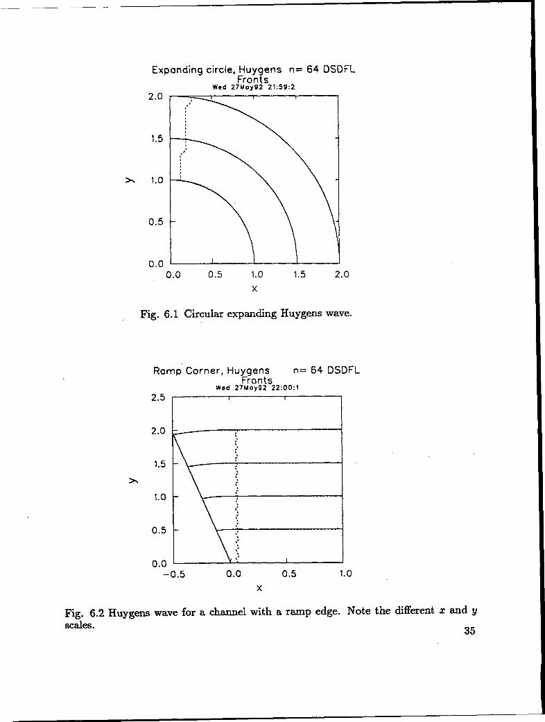
Fig. 6.2scales.

Expanding circle, :r;;f.ns n= 64 DSDFL

Wed 27 May92 21:59:2

2.0

1.5

h 1.0

0.5

0.0

,,’

.’,’

I

0.0 0.5 1.0 1.5

x

Fig. 6.1 Circular expanding Huygens

2.0

wave.

Romp Corner, Huygens n= 64 DSDFLFronts

Wed 27 Moy92 22:00:1

2.5

2.0

1.5

A

1.0

0.5

0.0

/ ::

\ :

Huygens

–0.5

wave for a

0.0

channel

0.5 1.0

x

with a ramp edge. Note the different zandy

35

Circle Corner, Hu gens{

n= 64 DSDFLrents

Wod 27 MoY92 22:00:2

2“5 ~

2.0

1.5

1,0

0.5

0.0–1.5 -1.0 -0.5 0.0 0.5 1.0

x

Fig. 6.3 Huygens wave forachannel with a circular edge.

The laboratory coordinates are

x =tsinu

Y =tcosu .

(2b) Channel with Ramp Edge

We have O = constant, (Y(t) = O, 0 negative. The flat initial wave is the step function

U=o, (=0,

u = -e , f>o;

we must have u =Oat( = O to match the edge. Again the solution is analogous to asimple centered rarefaction wave

36

The laboratory coordinates are

(2c) Channel with Circular Edge

We take a flat initial wave, with the left boundary a circle of radius r. The center ofthe circle is at x = –r, y = O, so that 00 = O. The angle O is a linear function of time

6 = –t/r ,

@’(t)= –l/r .

The governing equation isut + Uuc = I/r ,

i. e.: u =0 at t=O .

As in Problem 2b, we have the analog of a ID rarefaction wave moving into a constantstate,thistime noncenteredbecause of the gradualpullingaway of the boundary. Thecharacteristicsareparabolas.The characteristicf = _t2/2rthrough the originisthe headoftherarefactionwave. The solutionis

u=~, 4=&--t/r, t5t2/2r ,

u= t/r , fp=o , ~>t2/2r .

The laboratory coordinates of the wave front are

z=r[(su+c) cosu+(cu-s)sinu –1] ,

Y = r[(cu–s) cosu –(su+c) sinu] ,

CGCOS8, sssind, O= –t/r .

37

VII. CODE STRUCTURE

In this chapter, we describe the internal structure of the code itself. We begin byoutlining the main features of the numerical solution of the governing equations cent ainedin the FORTRAN source code. Next we describe the FCL control ille, the main loop of theprogram, and finally various pieces and subsystems of the program.

(1) The Numerical Solution

The governing equation, Eq. (3.1) is in general a parabolic PDE. To solve it, weuse the International Mathematical Software Library (IMSL) routine DPDES. For a c-net with n intervals, DPDES converts the PDE into a set of ODE’s, which it solves witha version of the Geara method. In each interval, the function ~(~) is fit with a cubicHermite polynomial with time-dependent coefficients. The coefficients are constrained bythe requirement that the function and its first derivative must be continuous at the endsof the interval (i.e., at the knots). These coefficients are the solution of the ODE’S. If n isthe specified number of intervals in ~ (as given in our ‘xnet’ line), there are 2n + 2 ODE’s,two between each knot and one at each boundary. The DPDES recipe evaluates the PDEat two Gaussian points per ~ interval to get the two collocation ODE’s for each interval.The boundary conditions replace the PDE at the two edges of the domain.

Let us first define some terms. We use the term time step to mean the time stepcovered by one call of DPDES. For each call, one specifies two times (tl and t2), and asksDPDES to integrate from tl to t2. In doing so, DPDES usually chooses several smallerinternal time steps of its own to satisfy the specified error tolerance. Ordinarily, we arenot concerned with these, but when we are, we will refer to them as DPDES internal timesteps. The time step At is calculated from the space step At. Its value is such that theratio At/A~ is approximately equal to the value of the fist item, xtrat, on the dialsline, for which we ordinarily take the value one. Decreasing xt rat improves the solutionquality for problems with curved boundaries and/or large changes in total shock arclength.The penalty incurred in increased computation time is modest. For some problems theDPDES time integration error tolerance, tol, needs to be decreased in order to maintainsolution symmetry. These improvements can be costly.

For our application, the two main shortcomings of DPDES are: (1) it has no way ofevaluating the integral over ~ in the B term of Eq. (3.1), and (2) it can apply a boundarycondition only at fixed ~.

We handle the l?-coefficient integral as follows: Before each time step we have # and~f at each ~, supplied by DPDES from the previous step. We calculate D(c); we nowhave all we need for the integrand. We then use a spline integration routine to calculatethe value of the integral at each (. It remains constant at this value throughout the nextDPDES step.

For most problems that we do, the total arclength along the shock changes with time.In order to use DPDES efficiently at any instant of time, we transform to a constant length

38

—

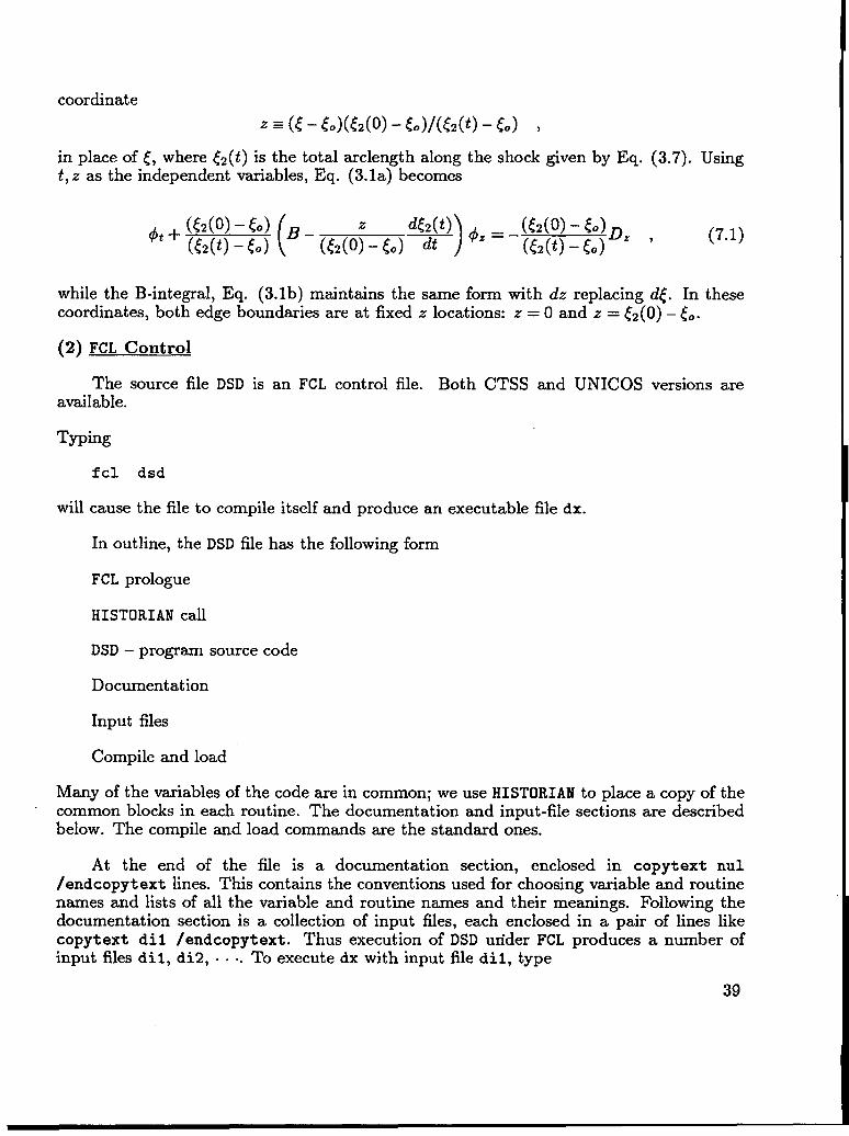
coordinate

z=(f–(o)(&(o) -&)/(&(t)-(o) ,

in place of ~, where (2(t) is the total arclength along the shock given by Eq. (3.7). Usingt, z as the independent variables, Eq. (3. la) becomes

+,+ ((2(0)- b) ( ) (MO)- to)~z ,(f(Z(t) #z = – ((2(~) – ( )((dt) -b) B- ((2(0;-(.) dt

(7.1)o

while the B-integral, Eq. (3. lb) maintains the same form with dz replacing d~. In thesecoordinates, both edge boundaries are at fixed z locations: z = O and z = $2(0) – to.

(2) FCL Control

The source file DSD is an FCL control file. Both CTSS and UNICOS versions areavailable.

Typing

fcl dsd

will cause the file to compile itself and produce an executable file dx.

In outline, the DSDfle has the following form

FCL prologue

HISTORIAN call

DSD– program source code

Documental ion

Input files

Compile and load

Many of the variables of the code are in common; we use HISTORIAN to place a copy of the“ common blocks in each routine. The documental ion and input-file sec~ions are described

below. The compile and load commands are the standard ones.

At the end of the file is a documentation section, enclosed in copytext nul

/endcOpytext fines.This contains the conventions used for choosing variable and routinenames and lists of all the variable and routine names and their meanings. Following thedocumentation section is a collection of input files, each enclosed in a pair of lines likecopyt ext di 1 /endcopyt ext. Thus execution of DSD under FCL produces a number ofinput files di.1, di2, . . .. To execute dx with input file dil, type

39

dx di = dil

The DSD code uses the following libraries:

SUBL – private library containing utilities and

CLAMS - LANL math library

DISSPLA – proprietary graphics package.

DPDES

(3) Main LooR

The main loop is in routine dsd. Before the loop begins, init and ic are called. Thesubroutine init calculates derived constants and initializes counts. The initial shock andthe edges are set up in ic.

The loop index kt goes horn 1 to nt, the number of computation steps. Computationroutines step and st epf are called in the loop. The subroutine step advances from thecurrent time to the next by calling DPDES and then advances other things, such as theedge 0’s, by centered forward difference. The coefficients needed by Eq. (7.1) for thenext time step are calculated in step and any intersection of the real and virtual edgesis determined there. The subroutine st epf sets the boundary conditions and calculatesthings after the step, such as the shock velocity and the ~-integral. The fist time throughthe 100P, with kt=l, step is skipped; thus stepf does its c~c~ation on the initial data.

The main output routines are out and outf. The subroutine out is called in theloop at display times. It prints the mesh, and then writes quantities from it on files forgraphical display at the end. The subroutine outf, called after the loop is complete, doesall the graphical display, getting the mesh quantities from the files written by out. Thesmall routine outp, called at each computation step, saves quantities from each “path,”such as the transverse-wave tracks, for display at the end by out f.

(4) Edves

The edge quantities are stored in two-dimensionalleft and right. The edge calculations are done in loops

arrays, with index j x 1,2 for the

j = 1,2.

Fimctionroutinesedge(&, j) furnishesthe angleO foredge ~ from the currentedgearclength&. In ic,equallyspacedarclengths& alongtheedge aregeneratedand storedin an array.The functionedge isthen calledforeach entryto generatea correspondingt9(&).Then lab iscalledto calculatearraysoflaboratoryedge coordinatesx and y from0 and &, from Eqs. (2.4).(Intheoutput wave diagram,theedgesareplottedfrom thesearrays.) Spline-fitcoefficientsforz(&) and ~(fe)arethen obtainedfrom spfit forlater

40

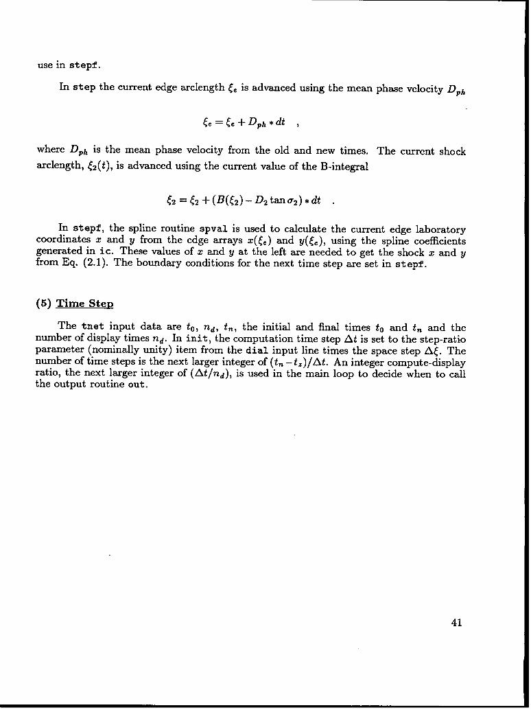
use in st epf.

In step the current edge arclength ~. is advanced using the mean phase velocity DP~

(e=[e+DP/t*dt ,

where DPh is the mean phase velocity from the old and new times. The current shock

arclength, (2(t), is advanced using the current value of the B-integral

(2 =gz+(~(tz)-Dztma2)*dt .

In st epf, the spline routine spval is used to calculate the current edge laboratorycoordinates x and y from the edge arrays Z( (e ) and y( fe ), using the spline coefficientsgenerated in ic. These values of x and y at the left are needed to get the shock z and yfrom Eq. (2.1). The boundary conditions for the next time step are set in st epf.

(5) Time Ste~

The tnet input data are tO, nd, t., the initial and final times tO and t. and thenumber of display times nd. In init, the computation time step At is set to the step-ratioparameter (nominally unity) item from the dial input line times the space step At. Thenumber of time steps is the next larger integer of (t. – t~)/At. An integer compute-displayratio, the next larger integer of (Ai/nd), is used in the main loop to decide when to callthe output routine out.

41

REFERENCES

1.

2.

3.

4.

5.

6.

7.

8.

9.

10.

J. B. Bdzil and D. S. Stewart, Phys. Fluids A. 1,1261-1267 (1989).

J. B. Bdzil, W. Fickett, and D. S. Stewart, “Detonation Shock Dynamics:A New Approach To Modeling Multi-Dimensional Detonation Waves,” inJ?roceedirws of The Ninth SvmDosium (International) on Detonation, Portland, OR,August 28-September 11989, pp. 730-742.

G. B. Whitham, Linear and Nonlinear Waveq (Wiley, New York, 1974).

B. D. Lambourn and D. C. Swift, “Application Of Whitham’s shockDynamics Theory To The Propagation Of Divergent Detonation Waves,” inProceedimzs of The Ninth Svmr)osium (International) on Deton ation, Portland, OR,August 28-Se@ember 11989, pp. 784-797.

J. Lee, P-A. Persson, and J. B. Bdzil, “Detonation Shock Dynamics of CompositeEnergetic Materials,” Phys. Fluids A., submitted, 1991.

J. B. Bdzil and D. S. Stewart, J. F2uid Mech. Vol. 171, 1-26 (1986).

W. Fickett, htroduc tion to Detonation Theorv (University of California Press,Berkeley, 1985).

C. W. Gear, umer ical Initial Value Problem s in Ord inarv D inferential F/auations(Prentice-Hall, Il&glewood Cliffs, 1971).

D. S. Stewart and J. B. Bdzil, Combwtion and Flame Vol. 72, 311-323 (1986).

R. Klein and D. S. Stewart, “The Relation Between Curvature, Rate State-Dependenceand Detonation Velocity? submitted, SIAM J. Appl. Math. (1992).

42

Appendix A. SCALING

Outside of this appendix we use scaled variables for which the CJ detonation velocityis unity and the CJ reaction time and length are unity or at least 0(1). In this appendixonly, we use plain symbols for physical (dimensional) quantities and barred symbols forscaled variables. Then we drop the bars for the rest of the report. To most simply illustratethe scaling, we take the k = O case (slab symmetry).

The governing equation, Eq. (3.1) is

(Al)

where ~ = +(. A typical D(K) relation is the linear form

D = DC~(l - cm) . (A.2)

Letting L and t be length and time, and using square brackets to denote “dimension of,”we have for the main dimensioned quantities

[D] = C/t ,[K= (#C]= l/c ,

[B] = c/t ,[a]=z .

(A.3)

For time, velocity, and distance scales, we take

t* = l/z , (A.4)

D* = DCJ ,~“ = D“t* ,

where Z is the reaction-rate multiplier. We assume that Z is such that the CJ reactiontime is Z-l or at least O(Z-l ). We define scaled variables

43

Applying these transformations, and dropping the bars gives Eq. (3.1) and

D=l–au

for the linear D(K) relation.

(A.5)

Appendix B. DETONATION FAILURE MODELS

A limited amount of theoretical work”!g exists to support the idea that D(K) is thepropagation law for weakly curved, diverging detonation shocks. The object of thesestudies was to examine how simple detonation models respond to weakly two-dimensionalperturbations of wavelength much longer than the reaction-zone lengthl”. They show thatif K is sufficiently small, D(K) describes the response of the shock to such perturbations.This is true even for explosives whose heat-release rates are moderately sensitive to thelocal state. These calculations do not show detonation extinction. Our development of theDSD model of detonation propagation was motivated by these results.

All real explosives exhibit detonation failure. For a number of important explosives

[

e.g., ammonium nitrate and fuel oil emulsion explosives and the triamino-trinitrobenzeneTATB) explosive PBX9502), it is observed that det&ation is extinguished when the

radius of curvature of the shock exceeds a critical value5. For these important materials,the detonation shock is smooth and broadly curved up to the onset of extinction. Weinterpret these observations as showing that D is a function of tc for these materials evenwhen the interaction between K and the state-dependence of the explosives’ heat-releaserate becomes large enough to produce extinction. Based largely on these experimentalobservations and with no theoretical support, we have extended our numerical algorithmto treat extinction.

(1) The Failure Model

The detonation failure model has two additional parameters: (1) a critical or failurecurvature, 6$ and (2) the spreading angle, af measured relative to the shock normal, ofthe failure wave along the shock. Consult Fig. 2.3 for a definition of the various angles.Our extinction model consists of the following six components:

44

(1)

(2)

(3)

(4)

(5)

(6)

detonation is stainable only where K < Kf,

K fit exceeds ~f on the physical boundary (edge), in response to abrupt changesin either b.c. type or edge shape,

the current b.c. on ~e (i.e., one of the standard set of b.c.) is replaced by a b.c.on the curvature, K = ~f when ss described in (2) K z ~f,

9

if at the onset of failure a < af, then the failure wave propagates intothe explosive and generates a virtual edge separating “dead” explosive fromdetonating explosive. This boundary is defined by O = #, – of, where K = Kfis the boundary condition that is applied,

if at the onset of failure a z of, then the failure wave follows the physical boundaryand o is not constrained, and

when an internal failure-wave boundary crosses the physical boundary, the failurecalculation is ended after K < ~f.

The defauli value of af is o= (i.e., the sonic angle). ~ f has no default value and alwaysneeds to be entered. We will demonstrate the properties oft his model by considering someexamples.

(2) Examdes

All the calculations that we describe use D = 0.8+ 0.2(1 – ~/tcf). We give the input

file for the first example only (Table B. I).

TABLE B.1. INPUT FILE di4a2fl

‘mm~ *Corner Turning (plane sym)‘! Plane ini.tial, hard right, two-side‘fluidt 3.0, 0.0‘Dkapt 3 1.00 0.80 0.50 !failure*edgel ●

~edger‘‘met*‘tnett‘tnet ~~ict

‘belt‘bcr’‘bcrt C*twav’

3 0.0 0.0 0.03 2.0 0.0 0.00.0 64 2.00.0 4 2.000.0 8 16.01 0.0 !line3 0.503 0.5011 0.0625

7.00 !file dp8crn7.00 !file dp9crn

sonicsonichardtwave (left bndry)

edials’ 0.25 0.001 0.000001

45

Example 1 (data file di4a2fl and Fig. B.1) shows detonation extinction in slabgeometry. The detonated explosive occupies the roughly “triangular” region whose cornersare at: (Z = O,y = O), (Z = 2,y = O), and (z = l,y = 6). Initially the shock is flat(O<z<2, y= O)andrunningat D=l. The failure waves that enter the system at(z = 0,~ = O) and (z = 2, y = O), continually erode the detonation until at t = 6.7 thedetonation is totally quenched. The chaindot lines are the failure-wave loci. The shockloci are shown at i = 0,2,4,6. The dashed line is the track of a right-facing acousticwave coming from the corner at (z = O,y = O). This problem used the parameter valuesKf = 1.0, Of = 0.5, and a= = 0.5.

Example 2 (Fig. B.2) retains the parameters of Example 1 with the exception that~f is increased to Kf = 2.0. Now the failure waves can propagate into the explosive only alimited distance. They are turned out at t = 1.14 and are flushed from the system at t = 3.0.Two small “dead” regions remain as the detonation proceeds up the slab. This calculationends at t = 7.0, at which time the detonation is about to enter the large piece of explosiveoccupying the region above y = 6.66. The shock loci are shown at t = 0,1,2,3,4,5,6,7.

Example 3 (Fig. B.3) uses the same parameters as Example 2. The plotting scale iscompressed. As the detonation emerges from the thin slab (see Fig. B.2 for a detailedpicture of the slab) into the large piece of explosive, it has great difficulty turning the90° corner. The detonation drives forward, spreading sideways only slowly. Most of theexplosive remains undetonated. This contrasts sharply with the perfect corner turning ofa Huygens wave. The shock loci are shown at t = 0,2,4,6,8,10,12,14,16.

Example 4 (Fig. B.4) uses the parameter values ~f = 2.0, of = 0.2, and a. = 0.2.These differ from the parameters in Example 2 in that both a and a. are reduced. The

{principal effect of this change is to decrease the speed of the fai ure waves along the shock.Now as the detonation enters the large piece of explosive occupying y ~ 6.66, the detonationspreads reasonably well. Two “dead” semi-elliptical zones remain at the corners. Asobserved experiment ally, the first arrival of the detonation along lines of constant x occursfor y >6.66, where the horizontal boundary is at y = 6.66. The shock loci are shown att = 0,2,4,6,8,10,12,14,16, 18.

Example 5 (Fig. B.5) uses the same parameters as does Example 2, except that thegeometry is axisymmetric. The most notable difference is the size of the “dead” zone: acylindrical shell of explosive remains undetonated.

‘ (3) Parameter Calibration

Our detonation-failure model qualitatively reproduces some of the well known featuresof extinction. Since no theoretical support exists for its use, it should be viewed as aphenomenological model. Nonetheless, when properly calibrated it can be a useful toolto help us predict when undesirable features such as “dead” zones will appear. We nowconsider a possible calibration strategy.

46

Of the two new parameters (K~ and of) that we require,Kj can be obtained from

“rate stick” data taken near the “failure diarnet cr.” This is obtained as part of the D(K)calibration to steady-state data. The failure-wave spreading parameter, crf can only beinferred from a time-dependent experiment. The corner-turning experiment shown inFig. B.4 can be used to estimate af. A highly-resolved numerical simulation of failingdetonation would also yield some insights. Clearly we expect that crf < a., because thespeed of the failure wave should not exceed the acoustic speed.

Corner Turning(pl;;oen;:m) n= 64 DSDFL

Wed 27 May92 22:39:4

8.0

6.0

h 4.0

2.0

0.0

4/“’\/ \mI \w,/ ,.,,.,., \

i,.-”,, I \

—

I

–1.0 0.0 1.0 2.0 3.0

x

Fig. B.1 The shock fronts for Example 1, showing detonation extinctioninan explosiveslab.Only the central“triangular”region detonates.

47

Corner Turning(plane sym) n= 64 DSDFL

8.0

6.0

> 4.0

2.0

0.0

FrontsWed 27 May92 22:45:5

.

/ -

/ w

/ \

..---,.,. ”

-..,”’,.-

,,,-., 4,..,.. I

–1.0 0.0 1.0 2.0 3.0

x

Fig. B.2 The shock fronts for Example 2. Small “dead” zones are found near theinput face y = O. Most of the explosive slab detonates.

Corner Turning(plgne sym) n= 64 DSDFL

20.0

15.0

h 10.0

5.0

0.0

FrontsWed 27 Moy92 22:59:1

1 1 1

–20.0 -10.0 0.0 10.0 20.0

x

Fig. B.3 The shock fronts for Example 3. As the detonation emerges into large pieceof explosive above y = 6.66, it is unable to turn the corner. Much of the materialremains undetonated. The parameters are those of Example 2.

48

Corner Turning(pl;:oen~:m) n= 64 DSDFL

Wed 27 May92 23:13:0

20.0

15.0

A 10.0

5.0

0.0 -._L_-20.0 -10.0 0.0 10.0 20.0

x

Fig. B.4Theshoclc fronts for Example 4. Whenaf ada~ me decre~ed from the

values used in Example 2 (i.e., setting of = a= = 0.2), the detonation turns the comer.Only small regions of “dead” explosive are left behind.

Corner Turning(axi–sym) n= 64 DSDFLFronts

Wed 27 Moy92 23:29:1

8,0

6.0

h 4.0

2.0

0.0

—

~

I-7+..-,...,”-

i ,= \..-

-2.0 –1.0 0.0 1.0 2.0

x

Fig. B.5 The shock fronts for Example 5. This is an axisymmetric problem that usesthe parameters of Example 2. A cylindrical shell of explosive remains undetonated.

49

*U.S. Government printing Of fic-: 1992-673-036/67024

Thisreporthasbeenreproduceddirectlyfromthebestavailablecopy.

Itk availabletoDOE andDOE contractorsfromtheOftlceofScientificandTechnicalInformation,P.O.BOX 62,OakRidge,TN 37831.Pricesareavailablefrom(615)576-8401,F13626-8401.

Itk availabletothepublicfromtheNationalTechnicalInformationService,U.S.DepartmentofCommerce,5285port Royid Rd.,Springfield,VA 22161.

Los Allamm Los Alamos National LaboratoryLos Alamos,New Mexico 87545