Embed Size (px)
Citation preview

33
Driving Innovation ♦ Delivering Results
Benefits of the NETL
Clean Coal and Carbon
Management Program
April 15, 2016
DOE/NETL-2016/0415
OFFICE OF FOSSIL ENERGY
National Energy Technology Laboratory

Analysis of Benefits of the NETL Clean Coal and Carbon Management Program
Disclaimer
This report was prepared as an account of work sponsored by an agency of the United States
Government. Neither the United States Government nor any agency thereof, nor any of their
employees, makes any warranty, express or implied, or assumes any legal liability or
responsibility for the accuracy, completeness, or usefulness of any information, apparatus,
product, or process disclosed, or represents that its use would not infringe privately owned rights.
Reference therein to any specific commercial product, process, or service by trade name,
trademark, manufacturer, or otherwise does not necessarily constitute or imply its endorsement,
recommendation, or favoring by the United States Government or any agency thereof. The views
and opinions of authors expressed therein do not necessarily state or reflect those of the United
States Government or any agency thereof.

Analysis of Benefits of the NETL Clean Coal and Carbon Management Program
Author List:
National Energy Technology Laboratory (NETL)
Charles Zelek
Supervisor, Energy Market Analysis Team
Energy Sector Planning and Analysis (ESPA)
Arun Iyengar, Allison Guinan, David Erne
Booz Allen Hamilton, Inc.
Christa Court
MRIGlobal
Lessly Goudarzi, Kara Callahan
Onlocation, Inc.
Randy Jackson, Caleb Stair, Xueting Zhao
West Virginia University
This report was prepared by Energy Sector Planning and Analysis (ESPA) for the United States
Department of Energy (DOE), National Energy Technology Laboratory (NETL). This work was
completed under DOE NETL Contract Number DE-FE0004001. This work was performed
under ESPA Task 342.04.24 with completion under MESA Task 2300.202.006.
The authors wish to acknowledge the excellent guidance, contributions, and cooperation of the
NETL staff, particularly:
Charles Zelek, Supervisor Energy Market Analysis Team, NETL Technical Monitor
Kristin Gerdes, Associate Director, Systems Engineering & Analysis
Evelyn Dale, NETL
Jose Benitez, NETL
DOE Contract Number DE-FE0004001

Analysis of Benefits of the NETL Clean Coal and Carbon Management Program
This page intentionally left blank.

Analysis of Benefits of the NETL Clean Coal and Carbon Management Program
i
Table of Contents
Executive Summary .........................................................................................................................1
1 Introduction ...................................................................................................................................4
2 CCS Market Landscape and Challenges .......................................................................................5
3 NETL’s RD&D to Addressing Challenges – Clean Coal and Carbon Management Program .....7 3.1 RD&D Programs for Coal Plants with Carbon Capture .......................................................7
3.2 NETL Carbon Storage Program RD&D .............................................................................11 3.3 RD&D Programs and Timelines .........................................................................................12
4 Technology Deployment Forecast and Benefits .........................................................................13
4.1 Analytical Approach ...........................................................................................................13 4.2 Scenarios Analyzed .............................................................................................................16 4.3 Results .................................................................................................................................18
5 Conclusion ..................................................................................................................................33
6 References ...................................................................................................................................35
Appendix A: CO2 Capture, Transport, Utilization, and Storage-National Energy Modeling
System Documentation ..........................................................................................................37 Appendix A.1: Introduction ......................................................................................................37 Appendix A.2: Representation of Coal CCS Retrofits into CTUS-NEMS ...............................43 Appendix A.3: Integration of NGCC CCS Retrofits into CO2 CTUS-NEMS ..........................48
Appendix A.4: Representation of New Build CCS in CO2 CTUS-NEMS ...............................57
Appendix A.5: Enhanced Representation of Industrial Sources in CO2 CTUS-NEMS ...........60 Appendix A.6: Transport Cost Model Formulation ..................................................................70 Appendix A.7: CO2 CTUS-NEMS Saline Cost Model Formulation ........................................79
Appendix A.8: Financial Functions in CO2 CTUS-NEMS .....................................................104 Appendix A.9: Estimating the Costs Associated with Financial Responsibility Post-
commercial Operation .....................................................................................................114
Appendix B: Econometric Input-Output Model Overview .........................................................117
Appendix B.1: Introduction ....................................................................................................117 Appendix B.2: Model Design .................................................................................................118
Appendix B.3: Input Data .......................................................................................................126
Appendix B.4: Model Outputs ................................................................................................132 Appendix B.5: Equations and Variables of the Macroeconomic Econometric Module .........133 Appendix B.6: References ......................................................................................................150

Analysis of Benefits of the NETL Clean Coal and Carbon Management Program
ii
Exhibits
Exhibit 2-1 LCOEs for plants starting up in 2020 (EIA AEO 2014 Reference Case) .................... 6 Exhibit 3-1 RD&D targets-coal power with carbon capture .......................................................... 8
Exhibit 3-2 LCOEs for plants starting up in 2035 (Carbon Mitigation Scenario, FE/NETL CTUS-
NEMS) .................................................................................................................................... 9 Exhibit 3-3 Minimum plant gate CO2 revenue required to incentivize CCS SOTA and 2nd
Generation costs of capture for existing coal fleet (NETL Carbon Capture Retrofit
Database) ............................................................................................................................... 10
Exhibit 3-4 Cost of saline storage of CO2 for all U.S. saline formations (2011 dollars) (FE/NETL
CO2 Saline Storage Cost Model) .......................................................................................... 12
Exhibit 3-5 RD&D timelines for coal power with carbon capture and carbon storage ................ 13
Exhibit 4-1 Schematic of the CTUS NEMS modeling process .................................................... 14 Exhibit 4-2 NETL ECIO model block diagram ............................................................................ 16 Exhibit 4-3 Salient scenarios analyzed ......................................................................................... 17 Exhibit 4-4 Salient assumptions for the scenarios analyzed in NEMS ......................................... 17
Exhibit 4-5 Electricity capacity mix timeline for the four scenarios without RD&D .................. 20 Exhibit 4-6 Electricity capacity mix timeline for the four scenarios with RD&D ....................... 21
Exhibit 4-7 Electricity generation mix timeline for the four scenarios without RD&D ............... 22 Exhibit 4-8 Electricity generation mix timeline for the four scenarios with NETL RD&D......... 23 Exhibit 4-9 Deployment of capacity with CO2 capture projected for all scenarios in 2025 and
2040 ....................................................................................................................................... 24
Exhibit 4-10 Electricity generation with CO2 capture projected for all scenarios in 2025 and 2040
............................................................................................................................................... 24 Exhibit 4-11 CO2 emissions from the power sector...................................................................... 25
Exhibit 4-12 Power sector CO2 emission reductions under different scenarios ........................... 26 Exhibit 4-13 CO2 captured for all scenarios in 2025 and 2040 .................................................... 27
Exhibit 4-14 Extended forecast for the storage of captured CO2 for the scenarios with and
without RD&D ...................................................................................................................... 28 Exhibit 4-15 Oil production from CO2 EOR operations ............................................................... 29
Exhibit 4-16 Electricity price forecasts ......................................................................................... 30 Exhibit 4-17 Power sector NG price forecasts .............................................................................. 31
Exhibit 4-18 CCS RD&D U.S. economic impacts and benefits cumulative through 2040*........ 32 Exhibit 4-19 CCS RD&D U.S. economic impacts under different discount rate assumptions for
the Reference Case (cumulative through 2040) .................................................................... 33
Exhibit A-1 CTUS flow diagram .................................................................................................. 38 Exhibit A-2 MDB data input tables .............................................................................................. 39 Exhibit A-3 MDB preprocessor tables .......................................................................................... 39 Exhibit A-4 User interface forms used in the MDB preprocessor ................................................ 40 Exhibit A-5 Categories of CCS capture in the CTUS model........................................................ 43
Exhibit A-6 Inputs and assumptions for unit cost calculation for Unit 491 ................................. 46 Exhibit A-7 Categories of CCS capture in the CTUS model........................................................ 48
Exhibit A-8 Plant 609 capital cost by generating unit in CTUS-NEMS plant database ............... 51 Exhibit A-9 Incremental capacity added with carbon capture (excluding coal retrofits) ............. 52 Exhibit A-10 Capacity with CO2 capture by technology type ...................................................... 53 Exhibit A-11 Volume of CO2 captured from power plants over time .......................................... 53 Exhibit A-12 Sources of CO2 for EOR ......................................................................................... 54
Analysis of Benefits of the NETL Clean Coal and Carbon Management Program
iii
Exhibit A-13 EOR activity............................................................................................................ 54 Exhibit A-14 CTUS-NEMS input files by type ............................................................................ 55 Exhibit A-15 New CCS coal-fired plants capital costs ................................................................. 57 Exhibit A-16 New CCS coal-fired plants heat rates ..................................................................... 58
Exhibit A-17 New CCS coal-fired plants fixed O&M costs......................................................... 58 Exhibit A-18 New CCS coal-fired plants variable O&M costs .................................................... 59 Exhibit A-19 Seven OGSM regions in NEMS ............................................................................. 61 Exhibit A-20 Industrial CO2 availability curve in NEMS ............................................................ 61 Exhibit A-21 NETL industrial CO2 time independent supply curve ............................................ 62
Exhibit A-22 Regional industrial CO2 availability curves ............................................................ 64
Exhibit A-23 Industrial CO2 price distribution ............................................................................. 65
Exhibit A-24 Comparison of industrial supply curves from the Midcontinent Region and their
representation in NEMS ........................................................................................................ 67 Exhibit A-25 CO2 purchased for EOR production ....................................................................... 69 Exhibit A-26 Mapping of NETL Transport Model capital cost variables to CTUS-NEMS
variables ................................................................................................................................ 70 Exhibit A-27 Mapping of Parker equation parameters to CTUS-NEMS parameter names ......... 72
Exhibit A-28 Values for transportation capital cost input parameters in CTUS-NEMS .............. 74 Exhibit A-29 Distribution of capital costs during construction .................................................... 74 Exhibit A-30 Values for transportation O&M cost input parameters in CTUS-NEMS ............... 76
Exhibit A-31 Mapping of NETL Transport Model cost components to CTUS-NEMS
counterparts in CTUSModIN.gdx ......................................................................................... 77 Exhibit A-32 Pipeline segment characteristics for crosswalk example ........................................ 77 Exhibit A-33 Comparison of CTUS-NEMS and NETL Transport Model output ........................ 78
Exhibit A-34 Comparison of NETL Transport Model to CTUS-NEMS transportation cost
formulation ............................................................................................................................ 78
Exhibit A-35 Pre-operational period capital investment: construction profile ............................. 79 Exhibit A-36 Mapping of plume area dependent costs (PADepCC) ............................................ 88 Exhibit A-37 Mapping of non-well dependent site costs (NW_PreOp) ....................................... 89
Exhibit A-38 Mapping of well dependent capital costs (WDepCC) ............................................ 93 Exhibit A-39 Mapping of well dependent operating expenses (OpExPerWell) ........................... 94
Exhibit A-40 Mapping of well dependent PISC costs (WellDepFinResp)................................... 95 Exhibit A-41 Mapping of three-year recurring capital costs (OP3YRCC) ................................... 97 Exhibit A-42 Mapping of five-year recurring capital costs (OP5YRCC) .................................... 98 Exhibit A-43 Mapping of CO2 volume dependent operating expenses (OpExPerTon) ............... 99
Exhibit A-44 Assumptions used in exogenous calculation exercise .......................................... 101 Exhibit A-45 Fixed new injection site costs ............................................................................... 101 Exhibit A-46 Well dependent costs ............................................................................................ 102 Exhibit A-47 Variable injection costs ......................................................................................... 102 Exhibit A-48 Total cost comparison ........................................................................................... 102
Exhibit A-49 Variance in saline storage unit costs between NETL Saline Model and CTUS-
NEMS ................................................................................................................................. 103
Exhibit A-50 CCR calculation numerical example .................................................................... 108 Exhibit A-51 Schedule of tax depreciation assuming double declining balance method changing
over to straight line; debt principal payments ..................................................................... 109 Exhibit A-52 Repeating investments numerical example ........................................................... 110
Analysis of Benefits of the NETL Clean Coal and Carbon Management Program
iv
Exhibit A-53 Impact of alternative assumptions ........................................................................ 112 Exhibit A-54 Periodic investments (years) ................................................................................. 112 Exhibit A-55 Periodic investments numerical example.............................................................. 113 Exhibit A-56 Periodic investments ............................................................................................. 113
Exhibit A-57 Total PV ................................................................................................................ 114 Exhibit A-58 Illustrative financial responsibility fund flows ..................................................... 115 Exhibit B-1 ECIO model configuration ...................................................................................... 118 Exhibit B-2 Industry aggregation scheme................................................................................... 122 Exhibit B-3 Definition of U.S. Census Bureau regions .............................................................. 129
Exhibit B-4 Map of U.S. Census Bureau regions ....................................................................... 130
Exhibit B-5 Flow chart of regionalization mechanism ............................................................... 131
Exhibit B-6 Identities of the Macroeconomic Econometric model ............................................ 135 Exhibit B-7 Endogenous variables of the Macroeconomic Econometric model ........................ 141 Exhibit B-8 Exogenous variables of the Macroeconomic Econometric model .......................... 145

Analysis of Benefits of the NETL Clean Coal and Carbon Management Program
v
Acronyms and Abbreviations
AEO Annual Energy Outlook
AES Advanced Energy Systems
AFR Annual financial responsibility
AoR Area of review
API American Petroleum Institute
BEA Bureau of Economic Analysis
Bbl Billions of barrels
BLS Bureau of Labor Statistics
Btu British thermal units
c/kWh Cent per kWh
CAF Capital cost adjustment factor
CCRD Carbon capture retrofit database
CCS Carbon capture and storage
CO2 Carbon dioxide
COE Cost of electricity
CRF Capital recovery factor
CTL Coal-to-liquids
CTUS Carbon capture, transport, utilization,
and storage
DDEPf Discounted depreciation factor
DDPP Discounted debt principal payment
DOE Department of Energy
DPP Debt paid in period
EC Econometric
ECIO Econometric Input Output
ECP Electricity capacity planning
EDC Escalation during construction
EFD Electricity fuel dispatch
EIA U.S. Energy Information
Administration
EMM Electricity Market Module
EPA U.S. Environmental Protection
Agency
EOR Enhanced oil recovery
ESPA Energy Sector Planning and Analysis
ETP Energy Technology Perspective
FCRF Fixed charge rate factor
FE Fossil Energy
FOAK First of a kind
FR Financial responsibility
GAMS General Algebraic Modeling System
GDP Gross domestic product
gdx GAMS data exchange
GHG Greenhouse gas
Gigatonnes 109 Tonnes
gmx GAMS script
GW Gigawatt
GWh Gigawatt-hour
h, hr Hour
IDC Interest during construction
IEA International Energy Agency
IEF Interest expense factor
IGCC Integrated gasification combined
cycle
in Inch, inches
IO Input-output
kW Kilowatts
kwh Kilowatt hour
lat latitude
LHS Left-hand side
LCOE Levelized cost of electricity
lon longitude
mi Mile, miles
mi2 Square miles
MIP Mixed-integer programming
MIT Mechanical integrity test
MMb/d Million barrels per day
MMBtu Million British thermal units
MMT Million metric tonne
MW Megawatts
MWh Megawatt-hour
NDI National Direct Impact
NEMS National Energy Modeling System
NETL National Energy Technology
Laboratory
NG Natural gas
NGCC Natural gas combined cycle
NGP Natural gas processing
NIPA National Income and Product
Accounts
NOAK Nth of a kind
NOI National Other Impacts
NPV Net present value
NTI National Total Impact
O&M Operation and maintenance
OPPB Office of Program Planning &
Benefits
OGSM Oil and Gas Supply Module
PC Pulverized coal
PISC Post injection site care
PV Photovoltaic
PVDO Present value of debt outstanding

Analysis of Benefits of the NETL Clean Coal and Carbon Management Program
vi
PWF Present worth factor
Qty Quantity
R&D Research and development
RD&D Research development and
demonstration
RDI Direct Regional Impacts
ROI Regional Other Impacts
ROW Right-of-way
RS Regional Shares
RTI Regional Total Impact
SOTA State of the art
TOC Total overnight cost
ton Short ton
Tonnes Metric tonne
Tcf Trillion cubic feet
U.S. United States
UDA Unit data analysis
UIC Underground injection control
VSP Vertical seismic profile
WVU West Virginia University
Yr Year

Analysis of Benefits of the NETL Clean Coal and Carbon Management Program
1
Executive Summary
Ensuring that the United States (U.S.) can continue to rely on clean, affordable energy from
abundant domestic fossil fuel resources is the primary mission of the National Energy
Technology Laboratory (NETL) Clean Coal and Carbon Management Program. In particular, the
program aims at hastening the commercialization of technologies that enable generation of
power from coal in an environmentally responsible way. The program’s mission is aligned with
the overall Department of Energy (DOE) strategy to reduce dependence on foreign energy
sources in addition to extending the availability of newly found natural gas resources, both of
which contribute to the enhancement of U.S. energy security in the short and long term.
A major focus of the Clean Coal and Carbon Management Program has been the mitigation of
greenhouse gas (GHG) emissions, specifically carbon dioxide (CO2), from power plants. NETL
is fostering the development of technologies, existing as well as novel, to minimize power plant
CO2 emissions through a combination of improvements in overall plant efficiency and
employment of CO2 capture technologies. The program also evaluates storage and utilization of
the captured CO2. Development of cost competitive low-carbon emission power plants with
carbon capture coupled with establishment of economically viable storage options form an
important aspect of the NETL Research Development and Demonstration (RD&D) programs.
Early carbon capture and storage (CCS) projects face several challenges, including climate
policy uncertainty, current high cost of CCS relative to alternatives, and initial deployment
barriers due to the risks generally associated with first-of-a-kind (FOAK) technologies. Domestic
regulatory policy and market opportunities are expected to play a significant role in driving CCS
projects. The U.S. Environmental Protection Agency (EPA) has issued regulations for new and
existing fossil fuel power plants, which provide a regulatory impetus for the inclusion of CCS.
(United States Environmental Protection Agency (EPA), 2010) Similarly, EPA regulations on
storage of CO2 in the subsurface and increased reporting requirements provide an initial
regulatory framework for CO2 storage; however, responsibility for the long-term management of
a storage site after it has received formal closure from the EPA still needs to be resolved in some
states. On the other hand, niche market opportunities such as enhanced oil recovery (EOR) using
CO2, may incentivize the deployment of new CCS systems. Many initial CCS projects have
been financed through the sale of captured CO2 for EOR providing a revenue stream to the
power project with a side benefit of increasing domestic oil production. Government incentives,
such as tax credits and subsidies, can also play an important supportive role in overcoming
significant FOAK system cost barriers.
The levelized cost of electricity (LCOE) of present state-of-the-art (SOTA) integrated
gasification combined cycle (IGCC) plants with 90 percent carbon capture, for example, is
generally 20–50 percent above that of dispatchable alternatives including natural gas systems,
nuclear, and wind. (U.S. Energy Information Administration (EIA), 2014) Potential cost offsets
through CO2 EOR revenue is not adequate to overcome the LCOE gap highlighting that the sale
of CO2 to EOR alone is limited in its ability to drive deployment of coal-fired plants with CCS.
Additionally, FOAK CCS projects exhibit much higher costs and risks than traditional coal or
natural gas power (without CCS), and the lack of an economy-wide price on CO2 emissions does
not create a market arena that is conducive to significant penetration of CCS. Government
involvement in CCS technology development and demonstration is consequently expected to
Analysis of Benefits of the NETL Clean Coal and Carbon Management Program
2
play a key role along with niche market opportunities and regulatory factors to enable CCS
deployments that can achieve the CO2 emission goals to limit climate impacts.
Accordingly, NETL has embarked upon an extensive RD&D program to develop technologies
for advanced coal power with CCS that will be technically viable and economically competitive,
while complying with increasingly strict environmental standards. The RD&D program sets
aggressive cost and performance goals for CCS technologies in the 2020 to 2030 timeframe to
facilitate competitive deployment of the technologies by 2040 and beyond.
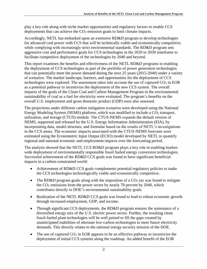
This report examines the benefits and effectiveness of the NETL RD&D programs in enabling
the deployment of CCS technologies as part of the portfolio of power generation technologies
that can potentially meet the power demand during the next 25 years (2015-2040) under a variety
of scenarios. The market landscape, barriers, and opportunities for the deployment of CCS
technologies were explored. The assessment takes into account the use of captured CO2 in EOR
as a potential pathway to incentivize the deployment of the new CCS system. The overall
impacts of the goals of the Clean Coal and Carbon Management Program in the environmental
sustainability of coal as a fuel for electricity were evaluated. The program’s benefits on the
overall U.S. employment and gross domestic product (GDP) were also assessed.
The projections under different carbon mitigation scenarios were developed using the National
Energy Modeling System (NEMS) platform, which was modified to include a CO2 transport,
utilization, and storage (CTUS) module. The CTUS-NEMS expands the default version of
NEMS, supported and released by the U.S. Energy Information Administration (EIA), by
incorporating data, model structure, and formulae based on the results of NETL’s investigations
in the CCS arena. The economic impacts associated with the CTUS-NEMS forecasts were
estimated using the Econometric Input Output (ECIO) model developed by NETL to quantify
regional and national economic and employment impacts over the forecasting period.
The analysis showed that the NETL CCS RD&D program plays a key role in enabling market-
wide deployment of environmentally responsible fossil fueled energy conversion technologies.
Successful achievement of the RD&D CCS goals was found to have significant beneficial
impacts in a carbon-constrained world:
Achievement of RD&D CCS goals complements potential regulatory policies to make
the CCS technologies technologically viable and economically competitive.
The RD&D program goals along with the imposition of a CO2 tax was found to mitigate
the CO2 emissions from the power sector by nearly 78 percent by 2040, which
contributes directly to DOE’s environmental sustainability goals.
Realization of the NETL RD&D CCS goals was found to lead to robust economic growth
through increased employment, GDP, and income.
Through significant CCS deployments, the RD&D program ensures the sustenance of a
diversified energy mix of the U.S. electric power sector. Further, the resulting clean
fossil-fueled plant technologies will be well poised to fill the gaps created by
unanticipated inabilities of alternate low-carbon technologies to meet future electricity
demands. This directly relates to the national energy security mission of the DOE.
The use of captured CO2 in EOR appears to be an effective pathway to incentivize the
deployment of initial CCS systems along the roadmap. An added benefit of the EOR
Analysis of Benefits of the NETL Clean Coal and Carbon Management Program
3
pathway is an associated increase in domestic oil production of approximately 4 billion
barrels cumulatively through 2040, which enhances U.S. energy security by potentially
displacing U.S. imports of foreign oil.
A well-developed large-scale CO2 storage infrastructure is necessary in order to achieve
and maintain the CO2 emissions reductions after the projection period. The carbon
storage program enables NETL to provide continued worldwide leadership to address the
technical and economic challenges facing CO2 storage in the short-term in non-EOR
markets as well as in the longer term saline storage scenarios.
The analysis demonstrates that along with the success of NETL RD&D programs, government
incentives, regulatory policies, and niche market opportunities are all essential elements in the
assurance of market-wide deployments of CCS technologies. Further, the projected carbon
mitigation scenarios require extensive new capacity of multiple low-carbon technologies,
emphasizing that an “all of the above strategy” must be undertaken to provide a hedge against
uncertainties in the cost of generation and infrastructure for each of the power generation
options.
Finally, the carbon mitigation scenario choices presented in this report provide one set of cost
projections, associated new capacity needs, and resulting deployments. However, actual market
factors, policy levers, and technology constraints are uncertain. Requirements of new capacity
will be impacted by factors such as coal plant retirements as the existing fleet ages and actual
carbon policies play out, nuclear retirements, uncertainties in NG prices, and growth in
electricity demand.

Analysis of Benefits of the NETL Clean Coal and Carbon Management Program
4
1 Introduction
The United States (U.S.) Department of Energy (DOE) programs have been actively pursuing the
research and development of clean energy conversion technologies to minimize their impact on
the environment. Ensuring that the U.S. can continue to rely on clean, affordable energy from
abundant domestic fossil fuel resources is the primary mission of the Clean Coal and Carbon
Management Program. In particular, the program aims at hastening the commercialization of
technologies that enable generation of power from coal in an environmentally responsible way.
Each of the program’s core focus areas -- Advanced Energy Systems, Carbon Storage, Carbon
Capture, and Crosscutting Research -- accelerate energy innovation through precompetitive
Research Development & Demonstration (RD&D), leveraging domestic and international
partnerships, and sustaining a world-leading technical workforce. The program’s mission is
aligned with the overall DOE strategy to reduce dependence on foreign energy sources in
addition to extending the availability of newly-found natural gas resources both of which
contribute to the enhancement of U.S. energy security in the short and long term.
A major focus of the Clean Coal and Carbon Management Program at the National Energy
Technology Laboratory (NETL) has been the mitigation of greenhouse gas (GHG) emissions,
specifically carbon dioxide (CO2), from the power plants, which has gained recent traction due to
increasing regulatory scrutiny. NETL is fostering the development of technologies, existing as
well as novel, to minimize power plant CO2 emissions through a combination of improvements
in overall plant efficiency and employment of CO2 capture technologies The program also
evaluates storage and utilization of the captured CO2. Development of cost competitive low-
carbon emission power plants with carbon capture coupled with establishment of economically
viable storage options form an important aspect of the NETL RD&D programs.
Early CCS projects face several challenges, including climate policy uncertainty, current high
cost of CCS relative to alternatives, and initial deployment barriers due to the risks generally
associated with first-of-a-kind (FOAK) technologies. Domestic regulatory policy and market
opportunities are expected to play a significant role in driving CCS projects. The U.S.
Environmental Protection Agency (EPA) has issued regulations for new and existing fossil fuel
power plants, which provide a regulatory impetus for the inclusion of CCS. (United States
Environmental Protection Agency (EPA), 2010) Similarly, EPA regulations on storage of CO2 in
the subsurface and EPA’s increased reporting requirements for monitoring the stored CO2
provide an initial regulatory framework for CO2 storage; however, responsibility for the long-
term management of a storage site after it has received formal closure from the EPA still needs
to be resolved in some states.
On the other hand, niche market opportunities may incentivize the deployment of new CCS
systems. Enhanced oil recovery (EOR) using CO2 provides a key opportunity for safe and
permanent storage of CO2. Many initial CCS projects have been financed through the sale of
captured CO2 for EOR providing a revenue stream to the power project and the side benefit of
increasing domestic oil production. Government environmental incentives, such as tax credits
and subsidies, can also play an important supportive role in overcoming significant FOAK
system cost barriers.
Accordingly, NETL has embarked upon an aggressive RD&D program to develop technologies
for advanced coal power with CCS that will be technically viable and economically competitive,
while complying with increasingly strict environmental standards. The RD&D program sets

Analysis of Benefits of the NETL Clean Coal and Carbon Management Program
5
aggressive cost and performance goals for CCS technologies in established time frames to
facilitate competitive deployment of the technologies in a future market.
This report examines the benefits and effectiveness of the NETL RD&D programs in enabling
the deployment of CCS technologies as part of the portfolio of power generation technologies
that can potentially meet the power demand during the next 25 years (2015-2040) under a variety
of scenarios. The market landscape, barriers, and opportunities for the deployment of CCS
technologies are also explored. The assessment takes into account the use of captured CO2 in
EOR as a potential pathway to incentivize the deployment of new CCS system. In addition, the
overall impacts of the goals of the clean coal and carbon management program in the
environmental sustainability of coal as a fuel for electricity, and the consequent program benefits
on the overall U.S. employment and gross domestic product (GDP) are elucidated.
2 CCS Market Landscape and Challenges
As reported by the Interagency Task Force on CCS,
While there are no insurmountable technological, legal, institutional, regulatory or
other barriers that prevent CCS from playing a role in reducing GHG emissions,
early CCS projects in the U.S. face economic challenges related to climate policy
uncertainty, FOAK technology risks, and the current high cost of CCS relative to
other technologies. (United States Environmental Protection Agency (EPA), 2010)
The EPA has issued regulations for new and existing fossil fuel power plants, which provide a
regulatory impetus for the inclusion of CCS. (United States Environmental Protection Agency
(EPA), 2010) Similarly, EPA regulations on storage of CO2 in the subsurface and increased
reporting requirements provide an initial regulatory framework for CO2 storage; however,
responsibility for the long-term management of a storage site after it has received formal closure
from the EPA still needs to be resolved in some states.
FOAK CCS projects exhibit much higher costs and risks than traditional coal or natural gas
power (without CCS), which along with the lack of an economy-wide price on CO2 emissions,
does not create a market arena that is conducive to FOAK projects. Early CCS projects will
likely depend on government environmental incentives, such as tax credits, to overcome
significant FOAK system cost barriers.
The economic challenges of the SOTA CCS technology are highlighted in Exhibit 2-1, which
shows a comparison of the levelized cost of electricity (LCOE) for new electric power capacity
using EIA’s cost and performance projections for the year 2020 in the 2014 Annual Energy
Outlook (AEO) Reference Case. (U.S. Energy Information Administration (EIA), 2014) As
shown, costs of IGCCa plants with 90 percent carbon capture, as reflected by EIA, are 20–50
percent above that of dispatchable alternatives (natural gas systems, nuclear, and wind with
a EIA reports cost and performance for supercritical pulverized coal (PC) with carbon capture, and while costs are lower than their estimated IGCC with carbon capture, it is not an option employed in AEO 2014.

Analysis of Benefits of the NETL Clean Coal and Carbon Management Program
6
natural gas back-up). Uncertainties associated with the variability of LCOE by region,b
including levelized natural gas pricesc as high as $8/MMBtu in some regions, do not close the
LCOE gap to directly enable coal plants with CCS (with the one exception being Photovoltaic
[PV] solar with natural gas back-up). The impact of an assumed plant gate revenue of $40/tonne
CO2 is reflected for the CCS plant types as a filled circle in Exhibit 2-1. This potential cost
offset is also not adequate to overcome the LCOE gap in the EIA projections for coal,
highlighting that the sale of CO2 to EOR alone is limited in its ability to drive deployment of coal
with CCS. Similarly, for natural gas combined cycle (NGCC) plants, EOR revenues alone will
not incentivize CCS, in part due to the lack of existing or proposed regulations that would
require CO2 capture on NGCC plants.
Exhibit 2-1 LCOEs for plants starting up in 2020 (EIA AEO 2014 Reference Case)d
Source: NETL
The options for an existing plant in a carbon mitigation scenario include: 1) continue to operate
business as usual and incur any cost on CO2 emissions, 2) retrofit for CCS using advanced
technology if the associated costs and risks are justified by potential CO2 revenues and/or
avoided costs on CO2 emissions, or 3) retire the existing plant and replace it with new capacity.
Retrofitting the existing fossil fuel power plant fleet with post-combustion capture CCS in
today’s policy environment provides the unique benefit of taking advantage of existing capital
b National average values and regional ranges are based on plants starting up in 2020 in the Reference Case; i.e.., regions with LCOEs for certain
plant types that are too high for deployment may not be reflected in the regional ranges.
c Natural gas prices used in LCOEs are levelized over 30 years, reflecting the projected real escalation of natural gas price over the economic life of the plant; thus, they are higher than the market price in the start-up year of the plant.
d Wind and solar PV with natural gas (NG) back-up are not reported by EIA, but are calculated in a simplified manner based on EIA LCOEs for
each stand-alone technology. NG back-up LCOEs reflect both pairing with NGCC (blue) and NG combustion turbines (red). No adjustments are made to NGCC cost and performance estimates to reflect inefficiencies and costs associated with load following.

Analysis of Benefits of the NETL Clean Coal and Carbon Management Program
7
assets. However, even SOTA post-combustion capture technology retrofits in most cases will not
be economically competitive with other power generation options in many markets.
In short, projected regulatory policy combined with other government incentives such as
subsidies and tax credits, while being necessary, are not sufficient for the sustenance of CCS
deployments in the energy marketplace. Additional government involvement in the form of
RD&D support plays an essential supplementary role in ensuring the commercial viability of the
CCS technology in the longer term.
3 NETL’s RD&D to Addressing Challenges – Clean Coal and
Carbon Management Program
Ensuring that the U.S. can continue to rely on clean, affordable energy from abundant domestic
fossil fuel resources is the primary mission of the Clean Coal and Carbon Management Program.
As such, the Fossil Energy (FE) coal research program is fully aligned with the goals of DOE’s
Strategic Plan-2015, sharing its primary objective, the prudent development of our Nation’s
natural resources. Each of the program’s core focus areas – Advanced Energy Systems, Carbon
Storage, Carbon Capture, and Crosscutting Research – accelerate energy innovation through
precompetitive RD&D, leverage domestic and international partnerships, and sustain a world-
leading technical workforce. This program seeks to develop affordable technology solutions that
link the full potential of abundant fossil energy resources with sound environmental stewardship.
To accomplish this mission, NETL conducts RD&D to develop technologies for advanced coal
power with CCS that will be technically viable and economically competitive, while complying
with increasingly strict environmental standards. By meeting aggressive cost and performance
goals for these technologies in established time frames, competitive deployment of the
technologies in a future market is anticipated. CCS deployment plays a key role in maintaining
environmental sustainability (domestically and internationally), contributing to economic
growth, and preserving energy security. NETL’s carbon storage program complements the
carbon capture technology developments by investigating, characterizing, and validating
potential domestic carbon storage options, both onshore and offshore.
3.1 RD&D Programs for Coal Plants with Carbon Capture
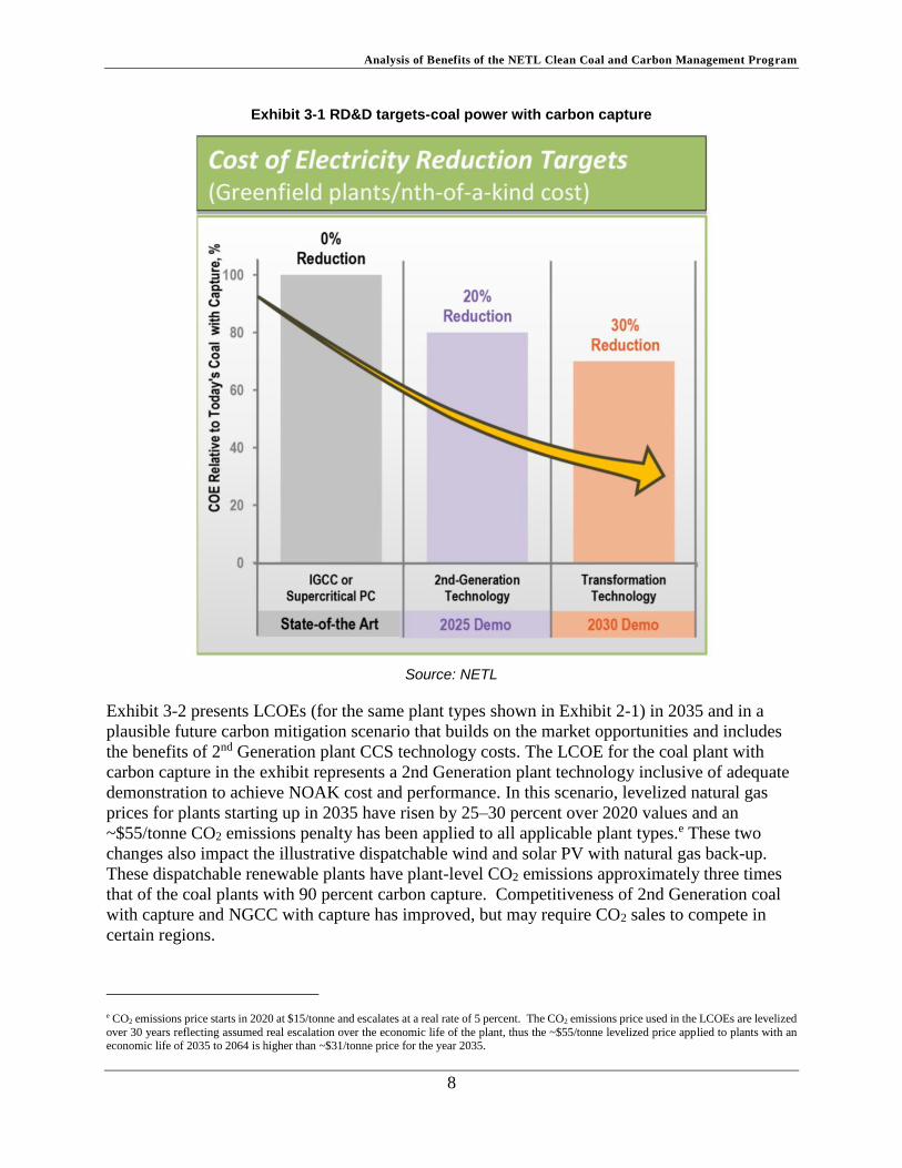
Technologies in both combustion and gasification pathways for advanced coal power with
carbon capture are being prepared for two future time frames with progressively aggressive cost
of electricity (COE) reduction targets. Second generation technologies are targeted to achieve a
20 percent reduction in COE compared to SOTA technology (See Exhibit 3-1) for coal-fired
power generation with CCS. This reduction is projected to enable coal power with CCS to be
competitively deployed, at least initially, as both new capacity and CCS retrofits in certain U.S.
regions when coupled with revenues for selling CO2 for EOR. Transformational technologies
coming online in the 2030 time frame are targeted to result in more than 30 percent reduction in
COE, which is required to enable and sustain market-wide CCS deployments.
Analysis of Benefits of the NETL Clean Coal and Carbon Management Program
8
Exhibit 3-1 RD&D targets-coal power with carbon capture
Source: NETL
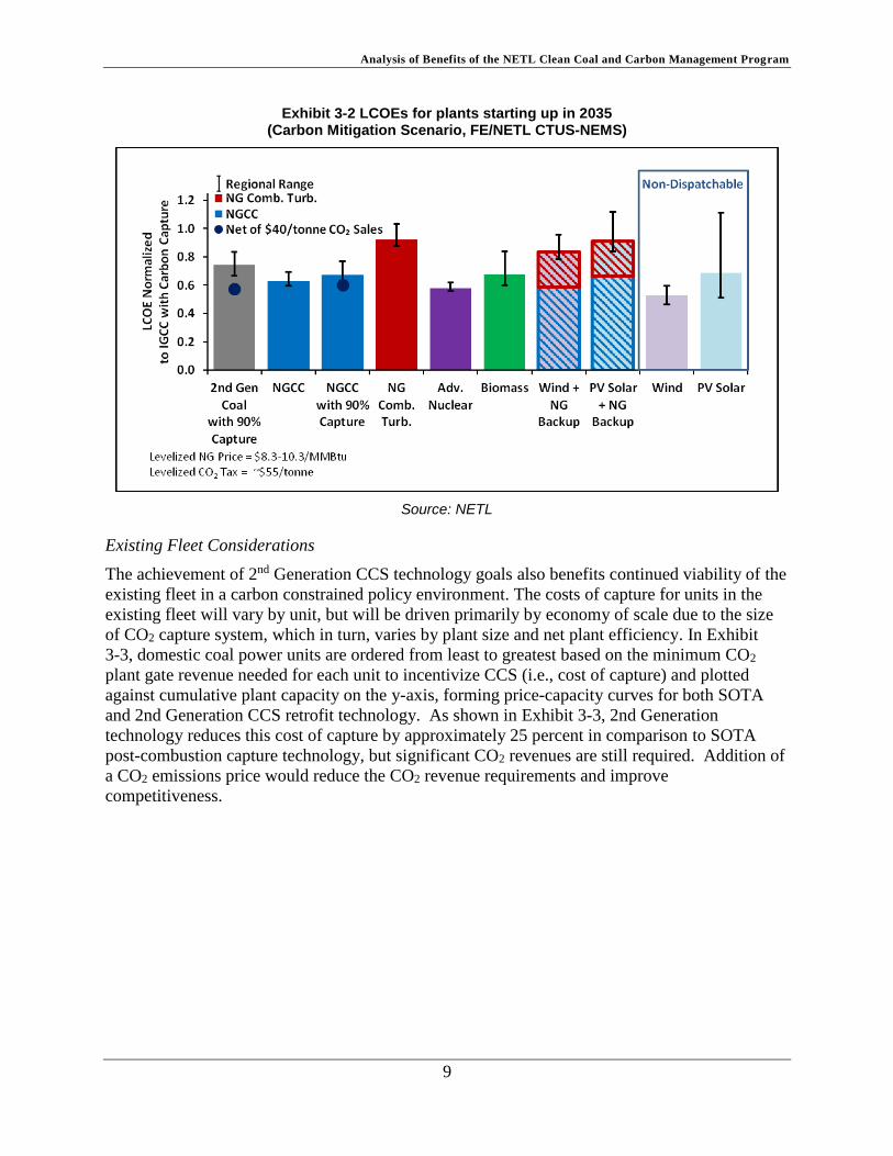
Exhibit 3-2 presents LCOEs (for the same plant types shown in Exhibit 2-1) in 2035 and in a
plausible future carbon mitigation scenario that builds on the market opportunities and includes
the benefits of 2nd Generation plant CCS technology costs. The LCOE for the coal plant with
carbon capture in the exhibit represents a 2nd Generation plant technology inclusive of adequate
demonstration to achieve NOAK cost and performance. In this scenario, levelized natural gas
prices for plants starting up in 2035 have risen by 25–30 percent over 2020 values and an
~$55/tonne CO2 emissions penalty has been applied to all applicable plant types.e These two
changes also impact the illustrative dispatchable wind and solar PV with natural gas back-up.
These dispatchable renewable plants have plant-level CO2 emissions approximately three times
that of the coal plants with 90 percent carbon capture. Competitiveness of 2nd Generation coal
with capture and NGCC with capture has improved, but may require CO2 sales to compete in
certain regions.
e CO2 emissions price starts in 2020 at $15/tonne and escalates at a real rate of 5 percent. The CO2 emissions price used in the LCOEs are levelized
over 30 years reflecting assumed real escalation over the economic life of the plant, thus the ~$55/tonne levelized price applied to plants with an economic life of 2035 to 2064 is higher than ~$31/tonne price for the year 2035.
Analysis of Benefits of the NETL Clean Coal and Carbon Management Program
9
Exhibit 3-2 LCOEs for plants starting up in 2035 (Carbon Mitigation Scenario, FE/NETL CTUS-NEMS)
Source: NETL
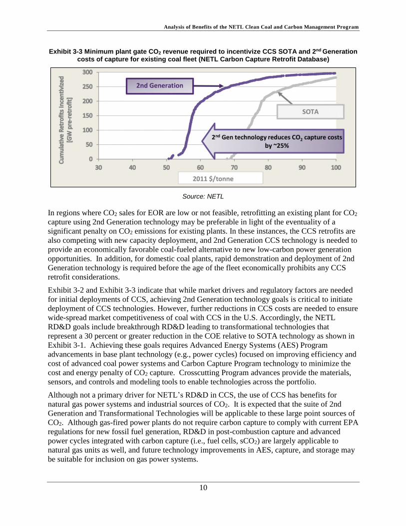
Existing Fleet Considerations
The achievement of 2nd Generation CCS technology goals also benefits continued viability of the
existing fleet in a carbon constrained policy environment. The costs of capture for units in the
existing fleet will vary by unit, but will be driven primarily by economy of scale due to the size
of CO2 capture system, which in turn, varies by plant size and net plant efficiency. In Exhibit
3-3, domestic coal power units are ordered from least to greatest based on the minimum CO2
plant gate revenue needed for each unit to incentivize CCS (i.e., cost of capture) and plotted
against cumulative plant capacity on the y-axis, forming price-capacity curves for both SOTA
and 2nd Generation CCS retrofit technology. As shown in Exhibit 3-3, 2nd Generation
technology reduces this cost of capture by approximately 25 percent in comparison to SOTA
post-combustion capture technology, but significant CO2 revenues are still required. Addition of
a CO2 emissions price would reduce the CO2 revenue requirements and improve
competitiveness.
Analysis of Benefits of the NETL Clean Coal and Carbon Management Program
10
Exhibit 3-3 Minimum plant gate CO2 revenue required to incentivize CCS SOTA and 2nd Generation costs of capture for existing coal fleet (NETL Carbon Capture Retrofit Database)
Source: NETL
In regions where CO2 sales for EOR are low or not feasible, retrofitting an existing plant for CO2
capture using 2nd Generation technology may be preferable in light of the eventuality of a
significant penalty on CO2 emissions for existing plants. In these instances, the CCS retrofits are
also competing with new capacity deployment, and 2nd Generation CCS technology is needed to
provide an economically favorable coal-fueled alternative to new low-carbon power generation
opportunities. In addition, for domestic coal plants, rapid demonstration and deployment of 2nd
Generation technology is required before the age of the fleet economically prohibits any CCS
retrofit considerations.
Exhibit 3-2 and Exhibit 3-3 indicate that while market drivers and regulatory factors are needed
for initial deployments of CCS, achieving 2nd Generation technology goals is critical to initiate
deployment of CCS technologies. However, further reductions in CCS costs are needed to ensure
wide-spread market competitiveness of coal with CCS in the U.S. Accordingly, the NETL
RD&D goals include breakthrough RD&D leading to transformational technologies that
represent a 30 percent or greater reduction in the COE relative to SOTA technology as shown in
Exhibit 3-1. Achieving these goals requires Advanced Energy Systems (AES) Program
advancements in base plant technology (e.g., power cycles) focused on improving efficiency and
cost of advanced coal power systems and Carbon Capture Program technology to minimize the
cost and energy penalty of CO2 capture. Crosscutting Program advances provide the materials,
sensors, and controls and modeling tools to enable technologies across the portfolio.
Although not a primary driver for NETL’s RD&D in CCS, the use of CCS has benefits for
natural gas power systems and industrial sources of CO2. It is expected that the suite of 2nd
Generation and Transformational Technologies will be applicable to these large point sources of
CO2. Although gas-fired power plants do not require carbon capture to comply with current EPA
regulations for new fossil fuel generation, RD&D in post-combustion capture and advanced
power cycles integrated with carbon capture (i.e., fuel cells, sCO2) are largely applicable to
natural gas units as well, and future technology improvements in AES, capture, and storage may
be suitable for inclusion on gas power systems.

Analysis of Benefits of the NETL Clean Coal and Carbon Management Program
11
3.2 NETL Carbon Storage Program RD&D
The Carbon Storage Program is developing and advancing carbon storage technologies that
support the scale-up and widespread global deployment of CCS, both onshore and offshore. The
technologies being developed and field tested in the near term are addressing the highest priority
of research challenges that need to be overcome for both saline and natural gas and oil reservoirs.
In addition, technologies being developed will verify carbon storage associated with CO2 EOR
operations.
EPA regulations on storage of CO2 in the subsurface along with EPA’s increased reporting
requirements for monitoring the stored CO2 provide an initial regulatory framework for CO2
storage; however, responsibility for the long-term management of a storage site after it has
received formal closure from the EPA still needs to be resolved in some states. This uncertainty
presents a significant financial challenge: as operators navigate the capital intensive stages prior
to operation to meet the stringent requirements of the permitting process, there is no guarantee of
project permits or certainty in the time it takes to obtain them. At the end of operations, the
transfer of liability for the storage site is another source of uncertainty, as there is a lack of
consensus on the appropriate party to be held responsible for long-term stewardship.
While great progress has been made in saline formation storage over the past decade,
considerable work remains to be done. In particular, there are relatively few large-scale CO2
storage projects in saline formations. These field projects are important for identifying and
resolving the technical challenges and risks associated with satisfying the evolving storage
regulatory environment. Large-scale projects as well as lab-scale and pilot-scale R&D are
needed to improve various aspects of carbon storage and reduce the risk of impacts to
underground sources of drinking water or the releases of CO2 to the atmosphere.
In addition to enabling the technical viability of CO2 storage and reducing the risks, successful
RD&D is anticipated to provide a cost benefit. For example, cost reductions are expected from a
number of R&D projects that integrate detailed empirical characterization using operational data,
monitoring results, and laboratory measurements with reservoir simulation models. Such
integrated frameworks can be used to optimize injection patterns and improve the placement of
monitoring equipment so as to increase storage capacity, reduce the size of the CO2 plume, and
lower monitoring costs. Exhibit 3-4 provides illustrative baseline storage costs (i.e., costs using
currently available technologies assuming these technologies perform in the field as expected)
generated with the FE/NETL CO2 Saline Storage Cost Model.f The model has 226 potential
saline storage formations, and the cost for storing CO2 in each formation was estimated along
with the mass of CO2 that can be stored in each formation. The formations were sorted from low
to high cost, and the cumulative mass of CO2 that can be stored for a given cost (or less) was
calculated. Exhibit 3-4 plots the cost (vertical axis) versus the cumulative CO2 that can be stored
at a given cost (horizontal axis) as well as the cost of storage reflecting the anticipated influence
of RD&D. To provide context, the exhibit provides an estimate of the CO2 from all fossil fuel
power plants and stationary industrial combustion sources if these sources captured 90 percent of
f The model and its documentation are available at http://www.netl.doe.gov/research/energy-analysis/analytical-tools-and-data/co2-saline-storage.

Analysis of Benefits of the NETL Clean Coal and Carbon Management Program
12
their CO2 emissions for 100 years.g Significant storage capacity is available for under $10/tonne
(in 2011 dollars) in certain regions. Exhibit 3-4 also indicates that successfully completed
RD&D could significantly expand the storage capacity available for under $10/tonne in 2011
dollars.
Exhibit 3-4 Cost of saline storage of CO2 for all U.S. saline formations (2011 dollars) (FE/NETL CO2 Saline Storage Cost Model)
Source: NETL
There is little data on actual regulatory requirements for CO2 storage projects, so the costs
provided in Exhibit 3-4 are based on best estimates of what regulators might require. NETL
assumed a two-year minimum for the permitting phase and the regulatory default of a 50-year
post injection phase for estimating the costs in this report. With the only cash-flow-positive
phase being operations, extension of the more uncertain phases such as permitting and site
closure can significantly impact project costs and appeal.
3.3 RD&D Programs and Timelines
The NETL RD&D timeline for a broad portfolio of technologies that are being readied to support
demonstration and deployment of advanced coal power with CCS beginning in 2025 is shown in
Exhibit 3-5.
g CO2 estimates are based on the EIA’s AEO 2014 projections through 2040 with extrapolation to 2115. (U.S. Energy Information Administration (EIA), 2014)
Analysis of Benefits of the NETL Clean Coal and Carbon Management Program
13
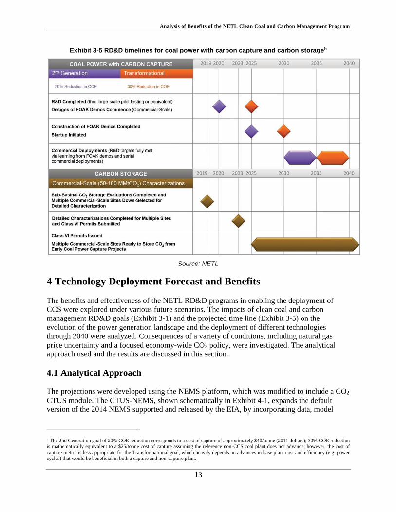
Exhibit 3-5 RD&D timelines for coal power with carbon capture and carbon storageh
Source: NETL
4 Technology Deployment Forecast and Benefits
The benefits and effectiveness of the NETL RD&D programs in enabling the deployment of
CCS were explored under various future scenarios. The impacts of clean coal and carbon
management RD&D goals (Exhibit 3-1) and the projected time line (Exhibit 3-5) on the
evolution of the power generation landscape and the deployment of different technologies
through 2040 were analyzed. Consequences of a variety of conditions, including natural gas
price uncertainty and a focused economy-wide CO2 policy, were investigated. The analytical
approach used and the results are discussed in this section.
4.1 Analytical Approach
The projections were developed using the NEMS platform, which was modified to include a CO2
CTUS module. The CTUS-NEMS, shown schematically in Exhibit 4-1, expands the default
version of the 2014 NEMS supported and released by the EIA, by incorporating data, model
h The 2nd Generation goal of 20% COE reduction corresponds to a cost of capture of approximately $40/tonne (2011 dollars); 30% COE reduction
is mathematically equivalent to a $25/tonne cost of capture assuming the reference non-CCS coal plant does not advance; however, the cost of
capture metric is less appropriate for the Transformational goal, which heavily depends on advances in base plant cost and efficiency (e.g. power cycles) that would be beneficial in both a capture and non-capture plant.

Analysis of Benefits of the NETL Clean Coal and Carbon Management Program
14
structure, and formulae based on the results of NETL’s investigations in the CCS
arena. (Appendix A)
Exhibit 4-1 Schematic of the CTUS NEMS modeling process
Source: NETL

Analysis of Benefits of the NETL Clean Coal and Carbon Management Program
15
The economic impacts associated with the CTUS NEMS forecasts were estimated using the
Econometric Input Output (ECIO) model. This model was developed by NETL to quantify
regional and national economic and employment impacts over a forecasting period. (Appendix
B) (National Energy Technology Laboratory (NETL), November, 2015) A block diagram of the
NETL ECIO model along with a list of its inputs from NEMS are shown in Exhibit 4-2. The
NETL ECIO formulation couples econometric (EC) modeling with the strengths of input-output
(IO) modeling. The EC model predicts final demands, primary factor demands, factor prices,
primary factor supplies, and their relationships within the U.S while the IO model projects
industry supply requirements and, in some cases, primary factor demands. The ECIO model
predicts the economic impacts of the following:
1. Construction of several types of power generation plants:
a. Scrubbed PC (with and without CCS)
b. IGCC (with and without CCS)
c. Combined cycle and advanced combined cycle (with and without CCS)
d. Onshore and offshore wind
e. Solar (PV and concentrated solar power)
f. Conventional and advanced nuclear
g. Distributed generation systems
2. Construction and operation and maintenance (O&M) of CO2 pipelines, CO2 storage at
saline sites, and CO2 EOR sites.
Additionally, the model also estimates the economic impacts of:
1. O&M associated with the types of power generation plants;
2. Retrofits of existing coal-fired and NGCC power generation plants for CCS;
3. Increased production of oil via EOR;
4. Changes in the technology mix that composes the power generation sector; and
5. Technical substitution effects of electricity, oil, and natural gas price changes and their
influence on prices of other commodities, as well as the consequent representations of
inter-industry structure.

Analysis of Benefits of the NETL Clean Coal and Carbon Management Program
16
Exhibit 4-2 NETL ECIO model block diagram
Source: NETL
4.2 Scenarios Analyzed
With the AEO 2014 case serving as the reference, multiple scenarios were analyzed using the
CTUS-NEMS model. (U.S. Energy Information Administration (EIA), 2014) Deployment and
other projections were made with and without the advantages of clean coal and carbon
management RD&D goals for each scenario. Constraints were imposed cumulatively to the
Reference Case to hypothesize a scenario pathway, shown in Exhibit 4-3, that could potentially
enable progressively larger CCS deployment rates.
Analysis of Benefits of the NETL Clean Coal and Carbon Management Program
17
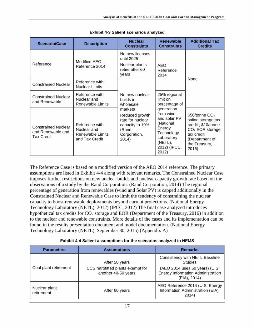
Exhibit 4-3 Salient scenarios analyzed
Scenario/Case Description Nuclear
Constraints Renewable Constraints
Additional Tax Credits
Reference Modified AEO Reference 2014
No new licenses until 2025
Nuclear plants retire after 60 years
AEO Reference 2014
None
Constrained Nuclear Reference with Nuclear Limits
No new nuclear builds in wholesale markets
Reduced growth rate for nuclear capacity to 10% (Rand Corporation, 2014)
Constrained Nuclear and Renewable
Reference with Nuclear and Renewable Limits
25% regional limit on percentage of generation from wind and solar PV (National Energy Technology Laboratory (NETL), 2012) (IPCC, 2012)
Constrained Nuclear and Renewable and Tax Credit
Reference with Nuclear and Renewable Limits and Tax Credit
$50/tonne CO2 saline storage tax credit ; $10/tonne CO2 EOR storage tax credit (Department of the Treasury, 2016)
The Reference Case is based on a modified version of the AEO 2014 reference. The primary
assumptions are listed in Exhibit 4-4 along with relevant remarks. The Constrained Nuclear Case
imposes further restrictions on new nuclear builds and nuclear capacity growth rate based on the
observations of a study by the Rand Corporation. (Rand Corporation, 2014) The regional
percentage of generation from renewables (wind and Solar PV) is capped additionally in the
Constrained Nuclear and Renewable Case to limit the tendency of constraining the nuclear
capacity to boost renewable deployments beyond current projections. (National Energy
Technology Laboratory (NETL), 2012) (IPCC, 2012) The final case analyzed introduces
hypothetical tax credits for CO2 storage and EOR (Department of the Treasury, 2016) in addition
to the nuclear and renewable constraints. More details of the cases and its implementation can be
found in the results presentation document and model documentation. (National Energy
Technology Laboratory (NETL), September 30, 2015) (Appendix A)
Exhibit 4-4 Salient assumptions for the scenarios analyzed in NEMS
Parameters Assumptions Remarks
Coal plant retirement
After 50 years
CCS retrofitted plants exempt for another 40-50 years
Consistency with NETL Baseline Studies
(AEO 2014 uses 60 years) (U.S. Energy Information Administration
(EIA), 2014)
Nuclear plant retirement
After 60 years AEO Reference 2014 (U.S. Energy Information Administration (EIA),
2014)

Analysis of Benefits of the NETL Clean Coal and Carbon Management Program
18
Parameters Assumptions Remarks
Nuclear licenses No new licenses until 2025 None
Oil and natural gas resources
50% reduction in gas and oil resources
EIA Low Resource Side Case (U.S. Energy Information
Administration (EIA), 2014)
EOR constraint 12 projects/year in 2015 increasing by
2 projects annually to maximum of 30/year (Koottlungal, 2012)
12 projects/year increasing by 1 project annually in AEO Reference
2014 (U.S. Energy Information Administration (EIA), 2014)
Carbon tax $15/tonne beginning in 2020 and
escalating by 5% annually
EIA (U.S. Energy Information Administration (EIA), 2014) has
$10/tonne and $25/tonne carbon tax side cases. A mid-carbon tax
was chosen
Retrofit assumptions
Eligibility threshold for retrofits: >100 MW capacity and <20,000 Btu/kWh
heat rate
The limits in AEO Reference 2014 (over 500 MW for retrofits and
maximum of 12,000 Btu/kWh for heat rate) did not allow economic evaluation for CCS capture (U.S. Energy Information Administration
(EIA), 2014)
Technology Learning
Without RD&D
Goals
50% reduction in learning from the AEO Reference 2014 value
Even though no research is funded in the U.S., it would be done
internationally and beneficially
With RD&D
Goals
As in AEO Reference 2014 Research is being funded
CCS Assumptions
Without RD&D Goals
No domestic CCS demo plants CCS technology available after 2030 Little R&D on CCS technology in U.S.
No funding for research
With RD&D Goals
NETL’s R&D program goals for CCS capture are applied to coal technology
for retrofits and new builds
CCS technology available after 2020
Clean coal and carbon management goals
4.3 Results
The results from both the CTUS-NEMS model and the ECIO models are presented and discussed
in this section. The constrained nuclear scenario along with the constrained nuclear and
renewable scenario results showed CCS deployment projections that were generally between the
Reference Case and the Constrained Nuclear and Renewable and Tax Credit Case.
4.3.1 Capacity and Generation
The timeline of the entire electricity capacity mix projected with and without RD&D for all
scenarios listed in Exhibit 4-3 are shown in Exhibit 4-5 and Exhibit 4-6, respectively. The
corresponding generation mixes are shown in Exhibit 4-7 and Exhibit 4-8 in a similar format. As
can be seen in these exhibits, constraining the renewable and nuclear technology deployments
Analysis of Benefits of the NETL Clean Coal and Carbon Management Program
19
have only a small impact on CCS deployments. Without RD&D, the nuclear technology
constraints tend to favor NGCC and renewable technologies, while the additional constraint of
limited renewable technology deployments changes the capacity/generation mix timelines by
only small amounts. In all cases, the prescription of NETL RD&D goals significantly enhances
the deployment of coal and NG CCS technologies, which displace renewable technologies and
NGCC plants without CCS, to meet the projected demand.
NETL RD&D programs have the potential to more than triple the CCS deployments by 2040. In
the Reference Case, achievement of RD&D program goals enables deployment of 69 GW of
capacity with CO2 capture by 2040 with nearly 45 percent (33 GW) in the form of new coal or
NG plants with CCS, as shown in Exhibit 4-9. The results indicate that a successful CCS RD&D
program enables sustained diversification of the energy in the U.S. electric power sector.
The additional imposition of a carbon tax credit has the most significant effect, resulting in a
nearly 200 percent increase in projected 2040 CCS deployments over the Reference Case. The
NETL RD&D program magnifies the impact of the carbon tax credit by nearly tripling the
potential CCS deployments to a total of 196 GW with 62 percent of coal plants including
~75GW of new coal plants with CCS. The corresponding generation with CO2 capture follows a
similar trend, as shown in Exhibit 4-10. The AEO Reference Case, also shown in the exhibit,
indicates that no significant deployment of CCS can be initiated without either a carbon policy or
RD&D. Exhibit 4-5, Exhibit 4-6, and Exhibit 4-9 show that a combination of regulatory policies,
government incentives, and RD&D programs similar to NETL’s are required to make fossil
fueled power plants with CCS, in general, and coal CCS, in particular, a significant part of the
U.S. electricity generation mix in the long term. Further, for the Reference Case with RD&D, the
results indicate a need for ~520 GW of new U.S. electricity generating capacity by 2040. This
assumes the availability of new capacity of over 300 GW of nuclear and renewables based power
generation to replace the coal plants being retired either due to end-of-life or due to compliance
requirements of the regulations on CO2 emissions. International scenarios, such as the
International Energy Agency’s (IEA) Energy Technology Perspectives (ETP) 2014 2DS
scenario, calls for 131 GW of U.S. CCS deployment (26 GW coal and 105 GW natural gas) and
>500 GW of non-U.S. CCS deployment through 2040 to meet targeted CO2 emissions
reductions. (International Energy Administration (IEA), 2014)
These results highlight that the projected carbon mitigation scenarios require extensive new
capacity of multiple low-carbon technologies, emphasizing that an “all of the above strategy”
must be undertaken to provide a hedge against uncertainties in the cost of generation and
infrastructure for each of these options and to ensure that the technology solutions are there to
support the electricity demand of a robust U.S. economy.

Analysis of Benefits of the NETL Clean Coal and Carbon Management Program
20
Exhibit 4-5 Electricity capacity mix timeline for the four scenarios without RD&D

Analysis of Benefits of the NETL Clean Coal and Carbon Management Program
21
Exhibit 4-6 Electricity capacity mix timeline for the four scenarios with RD&D

Analysis of Benefits of the NETL Clean Coal and Carbon Management Program
22
Exhibit 4-7 Electricity generation mix timeline for the four scenarios without RD&D

Analysis of Benefits of the NETL Clean Coal and Carbon Management Program
23
Exhibit 4-8 Electricity generation mix timeline for the four scenarios with NETL RD&D

Analysis of Benefits of the NETL Clean Coal and Carbon Management Program
24
Exhibit 4-9 Deployment of capacity with CO2 capture projected for all scenarios in 2025 and 2040
Exhibit 4-10 Electricity generation with CO2 capture projected for all scenarios in 2025 and 2040
Analysis of Benefits of the NETL Clean Coal and Carbon Management Program
25
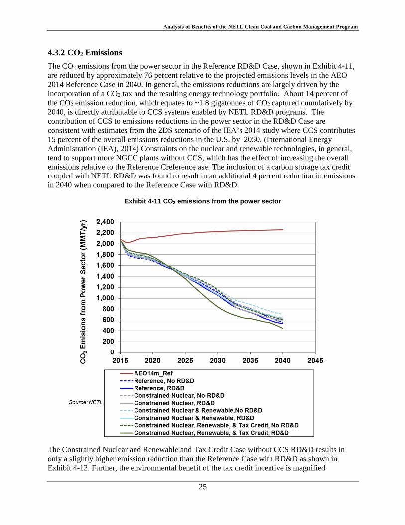
4.3.2 CO2 Emissions
The CO2 emissions from the power sector in the Reference RD&D Case, shown in Exhibit 4-11,
are reduced by approximately 76 percent relative to the projected emissions levels in the AEO
2014 Reference Case in 2040. In general, the emissions reductions are largely driven by the
incorporation of a CO2 tax and the resulting energy technology portfolio. About 14 percent of
the CO2 emission reduction, which equates to ~1.8 gigatonnes of CO2 captured cumulatively by
2040, is directly attributable to CCS systems enabled by NETL RD&D programs. The
contribution of CCS to emissions reductions in the power sector in the RD&D Case are
consistent with estimates from the 2DS scenario of the IEA’s 2014 study where CCS contributes
15 percent of the overall emissions reductions in the U.S. by 2050. (International Energy
Administration (IEA), 2014) Constraints on the nuclear and renewable technologies, in general,
tend to support more NGCC plants without CCS, which has the effect of increasing the overall
emissions relative to the Reference Creference ase. The inclusion of a carbon storage tax credit
coupled with NETL RD&D was found to result in an additional 4 percent reduction in emissions
in 2040 when compared to the Reference Case with RD&D.
Exhibit 4-11 CO2 emissions from the power sector
The Constrained Nuclear and Renewable and Tax Credit Case without CCS RD&D results in
only a slightly higher emission reduction than the Reference Case with RD&D as shown in
Exhibit 4-12. Further, the environmental benefit of the tax credit incentive is magnified

Analysis of Benefits of the NETL Clean Coal and Carbon Management Program
26
significantly by the success of NETL RD&D as shown by a considerable reduction in the CO2
emissions from the power sector in this case. NETL RD&D is primarily responsible for
capturing ~4.1 gigatonnes of CO2 cumulatively through 2040 by enabling considerable CCS
deployments in the Tax Credit Case.
Exhibit 4-12 Power sector CO2 emission reductions under different scenarios
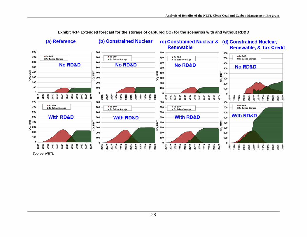
4.3.3 CO2 Storage and EOR
The CO2 captured as a result of the various CCS deployments is initially utilized in EOR
operations, which incentivizes them, as shown in Exhibit 4-13. Exhibit 4-14 shows the projected
distribution of the captured CO2 between EOR and saline storage sites for all the scenarios as a
function of time. Forecasts on the potential fate of the captured CO2 beyond 2040 based on the
static NEMS projected generation mix at 2040i are also included in the exhibit. NETL RD&D
clearly drives a significant increase in the total amount of CO2 stored, either from EOR
applications or due to direct saline storage.
i The NEMS projected generation mix at 2040 serves as the basis for these forecasts. The plants are assumed to capture the CO2 at the same rate until they retire and no new plants are assumed to be built in this forecast period.

Analysis of Benefits of the NETL Clean Coal and Carbon Management Program
27
Exhibit 4-13 CO2 captured for all scenarios in 2025 and 2040
In general, RD&D hastens the year in which saline formations become a dominant repository for
the captured CO2. However, significant CO2 storage in saline formations are projected only in
the years near the end or beyond the current forecasting period of 2040 for most of the scenarios.
Only the Carbon Storage Tax Credit Case, which results in significant CCS deployments in the
near-term, shows a dominant CO2 saline storage scenario, as early as 2030, due to the depletion
of the relatively small EOR capacity.
Regardless of the scenario, the CO2 storage projections beyond 2040, shown in Exhibit 4-14,
indicate that when oil production ceases at the EOR sites, CO2 will be diverted into a saline
formation for long-term storage subsequent to the satiation of the potential EOR storage
capacity. Accordingly, a well-developed large-scale CO2 storage infrastructure will be necessary
in order to initially achieve and then to maintain the CO2 emissions reductions reached both
during and after the projection period. The IEA 2DS forecast projects more than 690 GW of CCS
capacity to deploy worldwide through 2040. (International Energy Administration (IEA), 2014)
Many of the areas forecasted to have large CCS deployments do not have an EOR market in
which to sell captured CO2. This makes addressing the technical and economic challenges facing
CO2 storage in non-EOR projects an international issue, with technically viable, cost-effective
carbon storage playing an integral role in enabling the world to collectively mitigate climate
change. The carbon storage program is well positioned to continue to provide world-wide
leadership to help make this possible.
Analysis of Benefits of the NETL Clean Coal and Carbon Management Program
28
Exhibit 4-14 Extended forecast for the storage of captured CO2 for the scenarios with and without RD&D
Analysis of Benefits of the NETL Clean Coal and Carbon Management Program
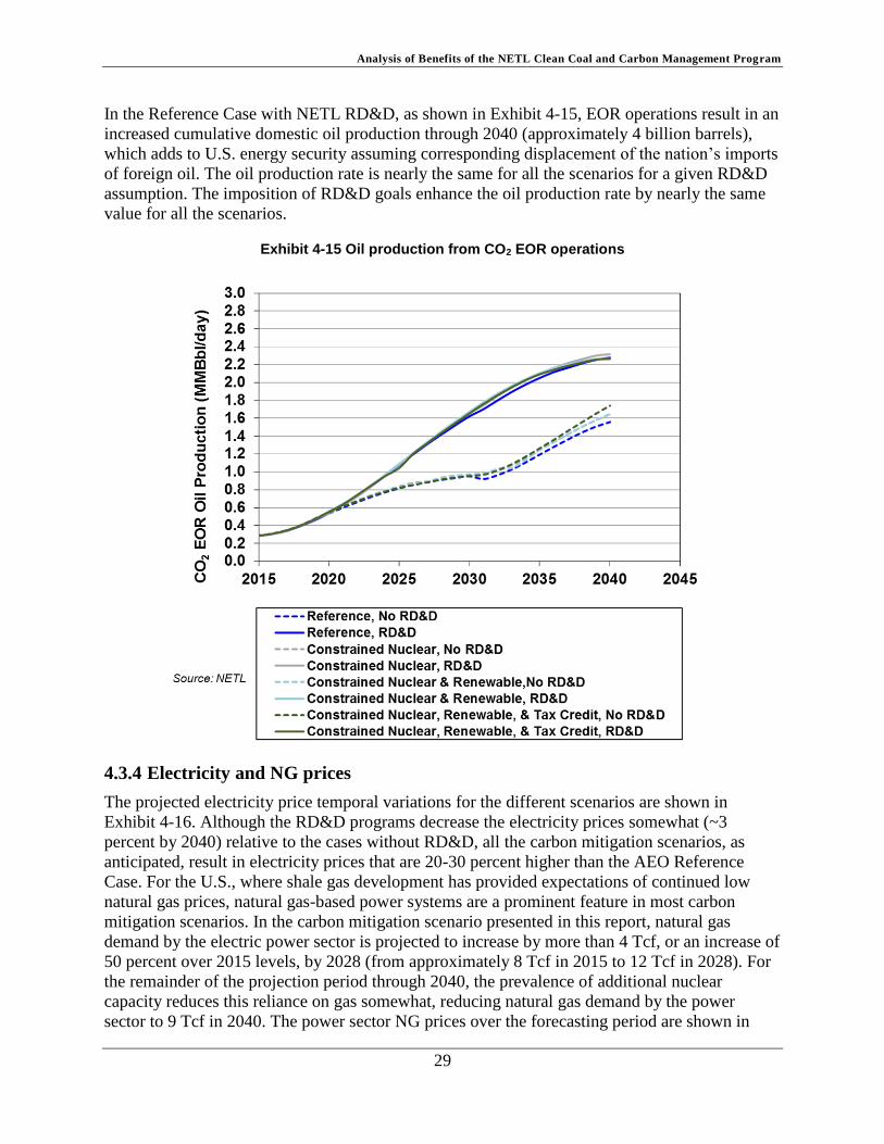
29
In the Reference Case with NETL RD&D, as shown in Exhibit 4-15, EOR operations result in an
increased cumulative domestic oil production through 2040 (approximately 4 billion barrels),
which adds to U.S. energy security assuming corresponding displacement of the nation’s imports
of foreign oil. The oil production rate is nearly the same for all the scenarios for a given RD&D
assumption. The imposition of RD&D goals enhance the oil production rate by nearly the same
value for all the scenarios.
Exhibit 4-15 Oil production from CO2 EOR operations
4.3.4 Electricity and NG prices
The projected electricity price temporal variations for the different scenarios are shown in
Exhibit 4-16. Although the RD&D programs decrease the electricity prices somewhat (~3
percent by 2040) relative to the cases without RD&D, all the carbon mitigation scenarios, as
anticipated, result in electricity prices that are 20-30 percent higher than the AEO Reference
Case. For the U.S., where shale gas development has provided expectations of continued low
natural gas prices, natural gas-based power systems are a prominent feature in most carbon
mitigation scenarios. In the carbon mitigation scenario presented in this report, natural gas
demand by the electric power sector is projected to increase by more than 4 Tcf, or an increase of
50 percent over 2015 levels, by 2028 (from approximately 8 Tcf in 2015 to 12 Tcf in 2028). For
the remainder of the projection period through 2040, the prevalence of additional nuclear
capacity reduces this reliance on gas somewhat, reducing natural gas demand by the power
sector to 9 Tcf in 2040. The power sector NG prices over the forecasting period are shown in

Analysis of Benefits of the NETL Clean Coal and Carbon Management Program
30
Exhibit 4-17 for all scenarios. Similar to the electricity prices, the NG prices in the carbon
mitigation scenarios are significantly higher than in the Reference AEO Case.
If natural gas prices and infrastructure costs remain low, CCS will be able to provide the
necessary CO2 reductions for greenfield and retrofit applications for an extensive U.S. NGCC
fleet. However, upward pressure on natural gas may be seen due to uncertainty in the ultimate
shale gas resources and due to the opportunities to export natural gas or to otherwise use it as a
chemical feedstock for higher value products. In this case, coal with CCS will have a critical
expanded role due to the vast domestic coal resources (481 billion short tons demonstrated
reserve basis as of 2013) and associated relatively stable coal prices.
Exhibit 4-16 Electricity price forecasts
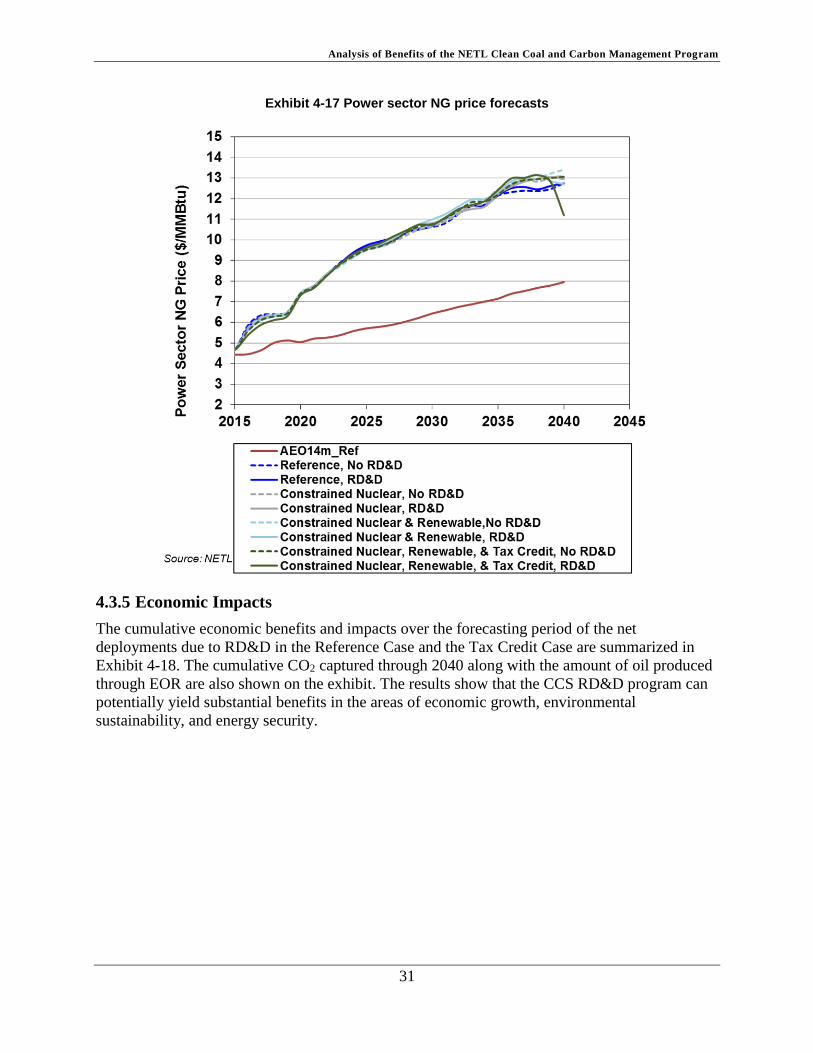
Analysis of Benefits of the NETL Clean Coal and Carbon Management Program
31
Exhibit 4-17 Power sector NG price forecasts
4.3.5 Economic Impacts
The cumulative economic benefits and impacts over the forecasting period of the net
deployments due to RD&D in the Reference Case and the Tax Credit Case are summarized in
Exhibit 4-18. The cumulative CO2 captured through 2040 along with the amount of oil produced
through EOR are also shown on the exhibit. The results show that the CCS RD&D program can
potentially yield substantial benefits in the areas of economic growth, environmental
sustainability, and energy security.

Analysis of Benefits of the NETL Clean Coal and Carbon Management Program
32
Exhibit 4-18 CCS RD&D U.S. economic impacts and benefits cumulative through 2040*
Benefit Area Metric Reference
Case
Constrained Nucl., Renew., & Tax Credit
Case
Economic Growth
Total Electricity Expenditure Savings (billion$) 65 144
Employment (million job years) 7.8 9.6
Income (billion$) 464 535
GDP (billion$) 1,130 1,316
Net Federal Government Tax Impacts (billion$) 77
Net State and Local Government Tax Impacts (billion$)
66
Environmental Sustainability
CO2 Captured at Coal and Gas CCS Facilities (Gigatonnes)
1.8 4.1
Energy Security Additional Domestic Oil Production via EOR (billion barrels)
4.1 3.9
*Dollar amounts expressed in real 2012 undiscounted dollars.
Higher discount rate assumptions tend to result in lower estimates of the economic impacts as
shown in Exhibit 4-19, which shows the economic impacts for discount rate assumptions of 3
and 7 percent for the cases shown in Exhibit 4-19.
The IEA also estimates that without CCS as a mitigation option, an additional $2 trillion will
have to be invested in the global electric power sector alone in order to limit the increase in
average global temperature to 2°C. (International Energy Administration (IEA), 2014) Of this
total, $460 billion will have to be invested in the U.S. power sector. (International Energy
Administration (IEA), 2014) These projected international deployments of CCS will both rely on
and greatly benefit from successful U.S. CCS RD&D.
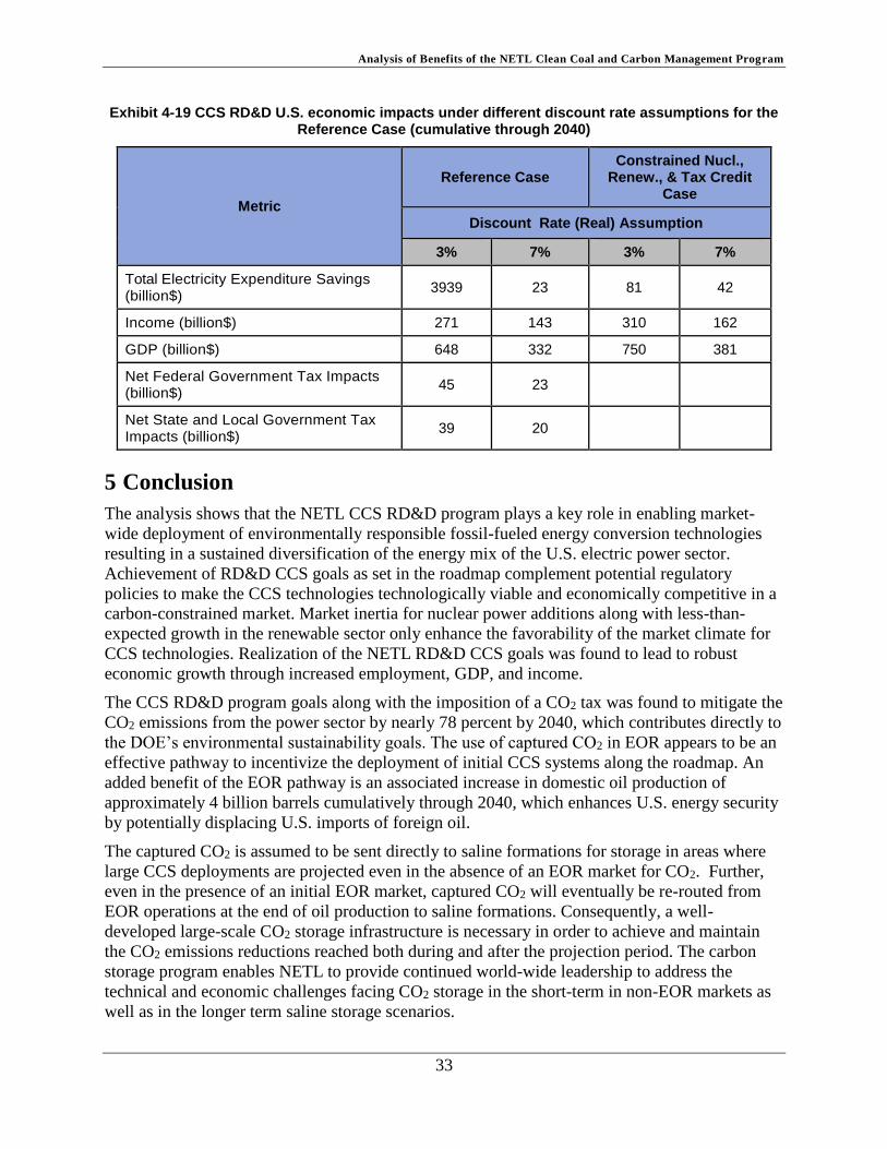
Analysis of Benefits of the NETL Clean Coal and Carbon Management Program
33
Exhibit 4-19 CCS RD&D U.S. economic impacts under different discount rate assumptions for the Reference Case (cumulative through 2040)
Metric
Reference Case Constrained Nucl.,
Renew., & Tax Credit Case
Discount Rate (Real) Assumption
3% 7% 3% 7%
Total Electricity Expenditure Savings (billion$)
3939 23 81 42
Income (billion$) 271 143 310 162
GDP (billion$) 648 332 750 381
Net Federal Government Tax Impacts (billion$)
45 23
Net State and Local Government Tax Impacts (billion$)
39 20
5 Conclusion
The analysis shows that the NETL CCS RD&D program plays a key role in enabling market-
wide deployment of environmentally responsible fossil-fueled energy conversion technologies
resulting in a sustained diversification of the energy mix of the U.S. electric power sector.
Achievement of RD&D CCS goals as set in the roadmap complement potential regulatory
policies to make the CCS technologies technologically viable and economically competitive in a
carbon-constrained market. Market inertia for nuclear power additions along with less-than-
expected growth in the renewable sector only enhance the favorability of the market climate for
CCS technologies. Realization of the NETL RD&D CCS goals was found to lead to robust
economic growth through increased employment, GDP, and income.
The CCS RD&D program goals along with the imposition of a CO2 tax was found to mitigate the
CO2 emissions from the power sector by nearly 78 percent by 2040, which contributes directly to
the DOE’s environmental sustainability goals. The use of captured CO2 in EOR appears to be an
effective pathway to incentivize the deployment of initial CCS systems along the roadmap. An
added benefit of the EOR pathway is an associated increase in domestic oil production of
approximately 4 billion barrels cumulatively through 2040, which enhances U.S. energy security
by potentially displacing U.S. imports of foreign oil.
The captured CO2 is assumed to be sent directly to saline formations for storage in areas where
large CCS deployments are projected even in the absence of an EOR market for CO2. Further,
even in the presence of an initial EOR market, captured CO2 will eventually be re-routed from
EOR operations at the end of oil production to saline formations. Consequently, a well-
developed large-scale CO2 storage infrastructure is necessary in order to achieve and maintain
the CO2 emissions reductions reached both during and after the projection period. The carbon
storage program enables NETL to provide continued world-wide leadership to address the
technical and economic challenges facing CO2 storage in the short-term in non-EOR markets as
well as in the longer term saline storage scenarios.

Analysis of Benefits of the NETL Clean Coal and Carbon Management Program
34
The analysis shows that along with the success of NETL RD&D programs, government
incentives, regulatory policies, and niche market opportunities are all key elements in the
assurance of market-wide deployments of CCS technologies. Further, the projected carbon
mitigation scenarios require extensive new capacity of multiple low-carbon technologies,
emphasizing that an “all of the above strategy” must be undertaken to provide a hedge against
uncertainties in the cost of generation and infrastructure for each of these options and to ensure
that the technology solutions are there to support the electricity demand of a robust U.S.
economy.
Finally, the carbon mitigation scenario choices presented in this report provide one set of cost
projections, associated new capacity needs, and resulting deployments. However, actual market
factors, policy levers, and technology constraints are uncertain. Requirements of new capacity
will be impacted by factors, such as coal plant retirements as the existing fleet ages and actual
carbon policies play out, nuclear retirements, uncertainties in NG prices, and growth in
electricity demand.

Analysis of Benefits of the NETL Clean Coal and Carbon Management Program
35
6 References
Department of the Treasury. (2016, February 9). Resource Center - Tax Policy. Retrieved
February 19, 2016, from https://www.treasury.gov/resource-center/tax-
policy/Documents/General-Explanations-FY2017.pdf
International Energy Administration (IEA). (2014). Energy Technology Perspectives,
Harnessing Electricity’s Potential.
International Energy Administration (IEA). (2014). Unpublished analysis from Energy
Technology Perspectives 2014. Paris: OECD/IEA.
IPCC. (2012). Renewable Energy Sources and Climate Change Mitigation. New York:
Cambridge University Press.
Koottlungal, L. (2012). 2012 Worldwide EOR Survey. Oil & Gas Journal, 110(4).
National Energy Technology Laboratory (NETL). (2012). Role of Alternative Energy Sources:
Solar Thermal Technology Assessment. Pittsburgh: DOE.
National Energy Technology Laboratory (NETL). (2016). CO2 Capture, Transport, Utilization,
and Storage-National Energy Modeling System Documentation.
National Energy Technology Laboratory (NETL). (May, 2015). NETL/WVU Econometric
Input-Output Model: Model Overview Report.
National Energy Technology Laboratory (NETL). (November, 2015). National Energy Modeling
System to Econometric Input-Output Model Translation Tool: Operator’s Guide.
National Energy Technology Laboratory (NETL). (September 30, 2015). CTUS-NEMS
Scenarios for the NETL Benefits Study.
Rand Corporation. (2014). Potential Influences on the Deployment of Nuclear Power in the U.S.
The Chicago Manual of Style (16 ed.). (2010). Chicago: University of Chicago Press.
U.S. Energy Information Administration (EIA). (2014, April). Annual Energy Oulook 2014 with
projections to 2040. Retrieved 11 April, 2016, from
http://www.eia.gov/forecasts/AEO/pdf/0383%282014%29.pdf

Analysis of Benefits of the NETL Clean Coal and Carbon Management Program
36
United States Environmental Protection Agency (EPA). (2010, August). Report of the
Interagency Task Force on Carbon Capture and Storage. Retrieved April 11, 2016, from
http://www.epa.gov/climatechange/Downloads/ccs/CCS-Task-Force-Report-2010.pdf

Analysis of Benefits of the NETL Clean Coal and Carbon Management Program
37
Appendix A: CO2 Capture, Transport, Utilization, and Storage-
National Energy Modeling System Documentation
Appendix A.1: Introduction
The carbon dioxide (CO2) Capture, Transport, Utilization, and Storage – National Energy
Modeling System (CTUS-NEMS) is a model, developed by Energy Sector Planning and
Analysis (ESPA) for the Department of Energy’s (DOE) National Energy Technology
Laboratory (NETL), that incorporates data, model structure, and formulae to reflect NETL’s
unique technical specifications that differ from the default version of the 2014 Annual Energy
Outlook (AEO14) National Energy Modeling System (NEMS) that is supported and released by
the Energy Information Administration (EIA).j This report documents the analytical approach
and output of CTUS-NEMS and catalogues and describes modeling assumptions, computational
methodologies, and data inputs. It serves as a reference for model analysts/users interested in the
construction and application of the CTUS module.
CO2 capture (from both existing power generation and industrial sources), transport, and storage
data developed by NETL was introduced into CTUS-NEMS. In addition, two models developed
by NETL (Fossil Energy [FE]/NETL CO2 Transport Cost Model, “NETL Transport Model,” and
FE/NETL CO2 Saline Cost Model, “NETL Saline Model”) have been translated into functional
equations in order to be represented in NEMS. This document describes how the NETL data is
incorporated into CTUS-NEMS as well as the formulations used to represent the NETL models.
Model Approach
The CTUS General Algebraic Modeling System (GAMS) model is a mixed-integer
programming (MIP) model that represents the interaction of CTUS amongst various capture
sites, injection sites, and pipeline options. Physical and economic data characterize each
functional category – capture, transport, utilization, storage, and monitoring. Scenarios can be
designed, and the model can be easily updated through changes in the data sets – limiting the
amount of code manipulation necessary to keep the model current.
Exhibit A-1 provides a flow diagram of the CTUS Model, illustrating the flow of data as well as
the interaction of CTUS GAMS with CTUS-NEMS (Electricity Capacity Planning [ECP]
Submodule).
CTUS-NEMS is initialized with “seed” data (default costs) obtained from running the CTUS
GAMS model in standalone mode (outside of NEMS), which produces an input database (in .gdx
format) for the NEMS ECP (called the CTSSoln.gdx). The data initialization routine establishes
representative costs for the transportation and storage of CO2 for each fuel region. The data
initialization routine (referred to as the MDB Preprocessor) establishes represented costs for
transportation and storage for each fuel region. The MDB Preprocessor is used to create the
input file (CTSinput.gdx) to the CTUS GAMS model.
j CTUS-NEMS is distinct from NEMS which is used by EIA for its AEO. While newer versions of NEMS have been released since the development of CTUS-NEMS, the CTUS submodule in CTUS-NEMS contains the most recent views of costs and technologies by NETL.

Analysis of Benefits of the NETL Clean Coal and Carbon Management Program
38
The NEMS uecp.f (Fortran code) reads in the “default” CTSSoln.gdx files, calls the CTUS
GAMS model, and reads in the CTSSoln.gdx file produced during the model run. The solution
from the CTUS model during the model run will include costs associated with new coal or gas
carbon capture and sequestration (CCS) plants and coal plants that the model has decided to
retrofit.
Exhibit A-1 CTUS flow diagram
Source: NETL
Data Management
The CTUS model is data driven. It is initialized via a MDB preprocessor that the user can edit
and includes numerous macros/forms set up to facilitate the production of the input gdx to the
CTUS model (called the CTSinput.gdx).
MDB Preprocessor
The input file that feeds the CTUS model (CTSinput.gdx) cannot be directly modified. This
provides a level of integrity to a model run – ensuring that inputs are not inadvertently changed.
Instead, a preprocessor (the “MDB Preprocessor”) is needed to transform raw data into the
CTSinput.gdx format. The raw data is housed in a Microsoft Access database that can be readily
modified by the user. The Microsoft Access database uses a series of routines (the “MDB
Preprocessor”) to transform the raw data into the CTSinput.gdx used by the model. Exhibit A-2
provides a list of each raw data table along with a brief description of its contents.
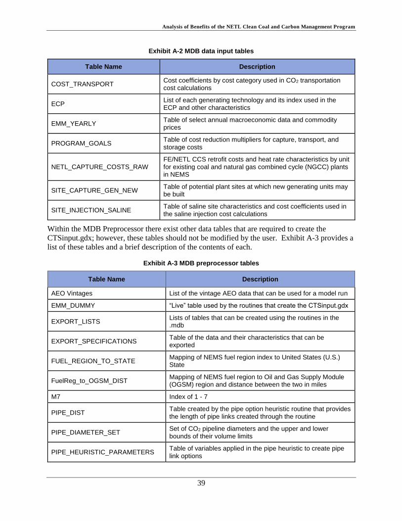
Analysis of Benefits of the NETL Clean Coal and Carbon Management Program
39
Exhibit A-2 MDB data input tables
Table Name Description
COST_TRANSPORT Cost coefficients by cost category used in CO2 transportation cost calculations
ECP List of each generating technology and its index used in the ECP and other characteristics
EMM_YEARLY Table of select annual macroeconomic data and commodity prices
PROGRAM_GOALS Table of cost reduction multipliers for capture, transport, and storage costs
NETL_CAPTURE_COSTS_RAW FE/NETL CCS retrofit costs and heat rate characteristics by unit for existing coal and natural gas combined cycle (NGCC) plants in NEMS
SITE_CAPTURE_GEN_NEW Table of potential plant sites at which new generating units may be built
SITE_INJECTION_SALINE Table of saline site characteristics and cost coefficients used in the saline injection cost calculations
Within the MDB Preprocessor there exist other data tables that are required to create the
CTSinput.gdx; however, these tables should not be modified by the user. Exhibit A-3 provides a
list of these tables and a brief description of the contents of each.
Exhibit A-3 MDB preprocessor tables
Table Name Description
AEO Vintages List of the vintage AEO data that can be used for a model run
EMM_DUMMY “Live” table used by the routines that create the CTSinput.gdx
EXPORT_LISTS Lists of tables that can be created using the routines in the .mdb
EXPORT_SPECIFICATIONS Table of the data and their characteristics that can be exported
FUEL_REGION_TO_STATE Mapping of NEMS fuel region index to United States (U.S.) State
FuelReg_to_OGSM_DIST Mapping of NEMS fuel region to Oil and Gas Supply Module (OGSM) region and distance between the two in miles
M7 Index of 1 - 7
PIPE_DIST Table created by the pipe option heuristic routine that provides the length of pipe links created through the routine
PIPE_DIAMETER_SET Set of CO2 pipeline diameters and the upper and lower bounds of their volume limits
PIPE_HEURISTIC_PARAMETERS Table of variables applied in the pipe heuristic to create pipe link options

Analysis of Benefits of the NETL Clean Coal and Carbon Management Program
40
Table Name Description
PIPE_OPT List of all pipe-link options (with diameter size in inches) created by the pipe option heuristic routine
PLTF860 The pltf860 table as used by EIA by AEO vintage
REGION_EMM Electricity Market Module (EMM) regions used in NEMS
SITE_CAPTURE_GEN_PSEUDO Location (latitude, longitude) of the centroid for each EMM region
SITE_CAPTURE_GEN_EXS Table of all existing coal units and their operating characteristics and retrofit costs
SITE_INJECTION_EOR_PSEUDO List of designated enhanced oil recovery (EOR) injection site for each OGSM region
SITE_TNODE2 List of each possible terminal node under which lies at least one injection site used in CTUS
SITE_TRANSSHIP List of each possible transshipment node used in CTUS
tmp_pipe_opt “Live” table used by the routines that create the CTSinput.gdx
The MBD Preprocessor uses a set of forms that provides an interface between the user and the
CTSinput.gdx generation process, each of which is described in Exhibit A-4 below.
Exhibit A-4 User interface forms used in the MDB preprocessor
Form Description
CTUS Existing Power Plant Selection Form
Captures data from the plant file selected by the user and merges this data with other tables used by other forms and routines for the generation of the CTSinput.gdx
Pipe Option Heuristic Form Generates a set of pipe options
GDX Exporter Form Exports tables to CTSinput.gdx
GAMS Code
The CTUS model is modeled using GAMS software. The model consists of four GAMS
program files:
● ctsshell.gms – control program used to set runtime option and call all of the other GAMS
programs. Calls the following GAMS code files in order:
o ctsprep.gms
o ctsmodel.gms
o ctsreprt.gms
● ctsprep.gms – reads in input data from CTSinput.gdx and CTSSavR.gdx and prepares
input coefficients for the MIP model. Data preparation steps include:
o Define index sets and parameters
o Assign new electricity unit builds to new plant site locations
o Calculate fixed and variable retrofit costs for existing coal and NGCC plants
o Calculate fixed and variable transportation costs for each pipeline link
o Calculate fixed and variable injection costs for each saline injection site

Analysis of Benefits of the NETL Clean Coal and Carbon Management Program
41
o Assign OGSM EOR CO2 demands to OGSM EOR injection sites
ctsmodel.gms – defines and solves the CTUS model
o Define the MIP model variables and constraints
o Set up solver options
o Solve the MIP model
● ctsreprt.gms – generates solution reports and calculates variables for use in the ECP
CO2 Capture Cost Data from Power Sources
NETL has developed costs to retrofit existing coal and NGCC power plants so they can capture
CO2. Similarly, NETL has developed costs to build new coal and new NGCC plants with carbon
capture technology. The coal retrofit cost data used in CTUS-NEMS come from NETL’s Coal
Carbon Capture Retrofit Database (CCRD) spreadsheet and model (Coal CCRD)k and is
addressed in Appendix A.2: Representation of Coal CCS Retrofits into CTUS-NEMS of this
document. The NGCC retrofit cost data comes from NETL’s NGCC CCRD spreadsheet
database and model, NGCC Unit Data Analysis (NGCC_UDA),l and is addressed in Appendix
A.3: Integration of NGCC CCS Retrofits into CO2 CTUS-NEMS.
Costs for building new coal power plants with CCS technology (CCS Coal) as well as heat rate
assumptions were developed by NETL.m Costs and heat rate assumptions for building new
NGCC power plants with CCS technology (CCS NGCC) were from EIA’s NEMS cost
assumptions. The treatment of both CCS Coal and CCS NGCC are addressed in Appendix A.4:
Representation of New Build CCS in CO2 CTUS-NEMS.
CO2 Capture Cost Data for Industrial Sources
NETL developed data that represent the expected cost of capture of CO2 and the potential
quantities available for capture from five industrial domestic sources: ammonia, cement, ethanol,
hydrogen refineries, and natural gas processing (NGP). NETL sought to use this data to develop
CO2 supply curves which would replace the industrial source data used by the EIA in the NEMS
and CTUS-NEMS. The modifications implemented to achieve this change are addressed in
Appendix A.5: Enhanced Representation of Industrial Sources in CO2 CTUS-NEMS.
CO2 Transport Costs
The NETL Transport Modeln was developed to estimate the costs associated with transfer of CO2
via pipeline under different length and volume scenarios. Reduced form equations were derived
from the NETL Transport Model for use in CTUS-NEMS. Appendix A.6: Transport Cost Model
Formulation describes the details and an example of the representation of the NETL Transport
Model in CTUS-NEMS.
k PC_CCRD_Unit Data_Analysis_rev0l_20140326_vhc.xlsx; not publically available due to proprietary nature of the data.
l NGCC_Unit_Data_Analysis_rev08C_20131101.xlsx; not publically available due to propriety nature of the data.
m Summer 2014 quick benefits run.xlsx.
n The FE/NETL CO2 Transport Cost Model is available online at: http://www.netl.doe.gov/research/energy-analysis/analytical-tools-and-data/co2-transport.
Analysis of Benefits of the NETL Clean Coal and Carbon Management Program
42
CO2 Saline Storage Costs
The CO2 saline storage cost formulation in CTUS-NEMS was revised to correspond with costs in
the NETL Saline Model.o To achieve this, a set of parameterized equations was developed that
provided a reasonable representation of the saline storage costs from the NETL Saline Model and
also accommodated the dynamics of the CTUS-NEMS model. The details of this documentation
can be found in Appendix A.7: CO2 CTUS-NEMS Saline Cost Model Formulation.
Financial Functions
Several financial functions are required in CTUS-NEMS to account for the financing of costs
and enable the proper accounting of financial flows over a variety of time horizons. A
description of each financial function introduced in CTUS-NEMS can be found in Appendix
A.8: Financial Functions in CO2 CTUS-NEMS. The specific financial treatment post injection
site care (PISC) costs are addressed in Appendix A.9: Estimating the Costs Associated with
Financial Responsibility Post-commercial Operation.
o The FE/NETL CO2 Saline Storage Cost Model is available online at: http://www.netl.doe.gov/research/energy-analysis/analytical-tools-and-data/co2-saline-storage.

Analysis of Benefits of the NETL Clean Coal and Carbon Management Program
43
Appendix A.2: Representation of Coal CCS Retrofits into CTUS-NEMS
Background
The carbon dioxide (CO2) Capture, Transport, Utilization, and Storage – National Energy
Modeling System (CTUS-NEMS) model uses the Department of Energy’s (DOE) National
Energy Technology Laboratory’s (NETL) Coal Carbon Capture Retrofit Database (CCRD)p as
the source for the coal carbon capture and sequestration (CCS) retrofit cost data. This section
describes how the NETL costs are represented in CTUS-NEMS and reports on the validation of
that representation.
Data Preparation
Coal-fired generation retrofit costs are stored at the unit level in both the CCRD and CTUS-
NEMS. Using the plant identification numbers and unit descriptions, costs are directly mapped
from the total overnight cost (TOC) field of NETL’s CCRD worksheet to the RetroBase variable
in the CTUS-NEMS (CTSinput.gdx) database.
Variable costs for Coal CCS retrofits are derived from the incremental operating cost
components in the CCRD and include fixed labor, fixed taxes and insurance, and variable costs
that assume a 100 percent capacity factor and are given on a dollar per short ton (2011$/ton)
basis. For use in CTUS-NEMS, the figures were adjusted for an assumed 75 percent capacity
factor and converted to dollars per tonne (2011$/tonne). Variable costs for coal retrofits are
stored in the CapCostVar variable in the CTUS-NEMS CTSinput.gdx database.
Within the CTUS submodule of CTUS-NEMS, carbon capture sources are assigned a numeric
index (Plant_Type) based on the fuel type of the source and whether it is a retrofit or new build
CCS technology. The identifiers and their assigned technologies are found in Exhibit A-5. The
indices allow for each CO2 source type to be tracked throughout CTUS-NEMS.
Exhibit A-5 Categories of CCS capture in the CTUS model
Fuel Type Build Type Plant_Type
Coal Retrofit 1
Coal New build 2
Natural gas Retrofit 3
Natural gas New build 4
Financial Treatment of the Capital Investments
Previous versions of CTUS-NEMS calculated and transferred an annual annuity of capital costs
from the CTUS Model to the Electricity Market Module (EMM). As part of the work under
ESPA 342.04.05, Sub-Activity 2, this methodology was changed so that capital costs for both
natural gas combined cycle (NGCC) retrofits and coal retrofits are now transferred from the
CTUS submodule to the EMM as overnight capital costs. All financial treatment of the
p PC_CCRD_Unit Data_Analysis_rev0l_20140326_vhc.xlsx; for NETL internal use only due to proprietary nature of vendor data.

Analysis of Benefits of the NETL Clean Coal and Carbon Management Program
44
overnight capital costs is performed within the existing construct of NEMS, leveraging economic
and financial assumptions from the Macroeconomic Activity Model (MAM) in NEMS. This
change ensures consistency in financial treatment of power plant capital investments across
technologies in the EMM.
Crosswalk and Unit Cost Reporting
As noted in Appendix A.2: Representation of Coal CCS Retrofits into CTUS-NEMS, the
overnight capital costs are taken directly from the CCRD and mapped into the RetroBase
variable of CTUS-NEMS.q The variable costs require a minor adjustment but are also easily
traced to their input variable (CapCostVar). Tracing the input cost assumption to the unit cost
figures (namely, “Unit_Capture_Costs-Fixed” and “Unit_Capture_Costs-Variable”) in the
CTUS-NEMS output reporting (CTSSoln.gdx), requires several more steps that occur in the
reporting submodule (ctsreprt.gms). The unit costs for capture, as reported in the Unit Cost
table, apply only to coal and NGCC retrofit costs and represent the levelized cost per tonne of the
item on a unit basis for coal-fired generation and plant basis for NGCC plants. In its simplest
form, the levelized unit cost is the discounted (present value [PV]) cost (capital and variable)
divided by the discounted flow of CO2. The discounted cost flows in the model are captured in
the following equations:
For Capital Costs:
CostWorkCapCostType = SrcCapCost / ∑(CAPTUREDt * PVt) (eq. 1)
Where:
CostWorkCapCostType = unit cost of the retrofit (2012$/tonne)
CostType = fixed or variable, depending on the cost used as a basis for the
calculation. In this equation, it is set for capital costs and is
therefore “fixed.”
SrcCapCost = the capital cost of the retrofit, discounted to the beginning of the
planning horizon (2012$ million)
CAPTURED = the stream of CO2 captured from the retrofit plant (MMT)
PV = the multiplier that yields the present value of a cost in a given
year to the beginning of the planning horizon (unitless)
t = model year (yr)
For reporting, the CostWorkCapCostType variable is converted from 2012$/tonne to 2007$/tonne
using the gross domestic product (GDP) indicesr from those years (1.782 and 1.64, respectively).
q For use in the linear program in the EMM, the RetroBase costs are converted to 1987 dollars (1987$). r GDP indices are taken from the MACOUT_MC_PPGDP variable in NEMS.
Analysis of Benefits of the NETL Clean Coal and Carbon Management Program
45
Calculation of SrcCapCost
SrcCapCost is based on the capital cost stored in the RetroBase variable. Because RetroBase is
in 2011$ million, the cost must be converted to 2012$ using GDP indices (1.782 for 2012 and
1.751 for 2011).
SrcCapCost = RetroBase * GDP(2012) / GDP(2011) * PV* FCRF*CAF * CRF
(eq. 2)
Where:
RetroBase = the overnight capital cost of a coal retrofit (2011$ million)
GDP(year) = the gross domestic product index for a given year (unitless)
PV = the multiplier that yields the present value of a cost in a given year to the
beginning of the planning horizon (unitless)
FCRF = fixed charge rate factor (see Appendix A.8: Financial Functions in CO2
CTUS-NEMS for detailed discussions on this and other financial factors)
(unitless)
CAF = capital cost adjustment factor (see Appendix A.8: Financial Functions in
CO2 CTUS-NEMS for detailed discussions on this and other financial factors)
(unitless)
CRF = capital recovery factor (see Appendix A.8: Financial Functions in CO2
CTUS-NEMS for detailed discussions of this and other financial factors)
(unitless)
For Variable Costs:
CostWorkCapCostType = CaptureCost (eq. 3)
Where:
CostWorkCapCostType = unit cost of the retrofit (2012$/tonne)
CostType = fixed or variable, depending on the cost used as a basis for the
calculation. In this equation, it is set for variable costs and is
therefore “variable”
CaptureCost = the capital cost of the retrofit, discounted to the beginning of the
planning horizon (2012$/tonne)
Calculation of CaptureCost
CaptureCost is based on the capital cost stored in the CapCostVar variable. Because
CapCostVar is in 2011$/tonne, the cost must be converted to 2012$/tonne using GDP indices
(1.782 for 2012 and 1.751 for 2011).
CaptureCost = CapCostVar * GDP(2012) / GDP(2011) (eq. 4)
Where:

Analysis of Benefits of the NETL Clean Coal and Carbon Management Program
46
CapCostVar = the variable cost per tonne of a coal retrofit (2011$/tonne)
GDP(year) = the gross domestic product index for a given year (unitless)
Using NEMS Unit (IGRP) 491 as an example, this calculation is illustrated for capital (fixed)
and variable costs. The inputs and assumptions are in Exhibit A-6.
Exhibit A-6 Inputs and assumptions for unit cost calculation for Unit 491
Input/Assumption Value
Unit ID 491
Year of retrofit 2025
GDP(2012) 1.782
GDP(2011) 1.751
GDP(2007) 1.640
PV (2025) 0.467
FCRF 0.175
CAF 1.211
CRF 10.081
CAPTURED CO2 (MMT/yr) 4.153 from 2025-2040
CostType Fixed Variable
RetroBase (2011$ million) 1472.21 N/A
CapCostVar (2011$/tonne) N/A 7.405
Reported unit cost (2007$/tonne) 66.45 6.94
For Capital Costs, SrcCapCost is calculated:
SrcCapCost = 1472.21 *(1.782 / 1.751) * 0.467 *0.175 * 1.211 * 10.81
= 1499.16 (2012$ millions)
and then
CostWorkCapCostType = 1499.16 / ∑(4.153t * PVt); for t = 2025 to t = 2040
= 1499.16 / 20.754
= 72.23 (2012$/tonne)
Adjusting from 2012$ to 2007$:
72.23 * (1.64 / 1.782) = 66.47 (2007$/tonne)
This calculated cost of $66.47/tonne is less than 1 percent different than the $66.45/tonne
reported cost from the model due to rounding errors.
For Variable Costs, CaptureCost is calculated:
CaptureCost = 7.405 * (1.782 / 1.751)
Analysis of Benefits of the NETL Clean Coal and Carbon Management Program
47
= 7.536 (2012$/tonne)
and then
CostWorkCapCostType = 7.536 * (1.64/1.782)
= 6.94 (2007$/tonne)
The calculated cost of $6.94/tonne is the same as the $6.94/tonne reported cost from the model.
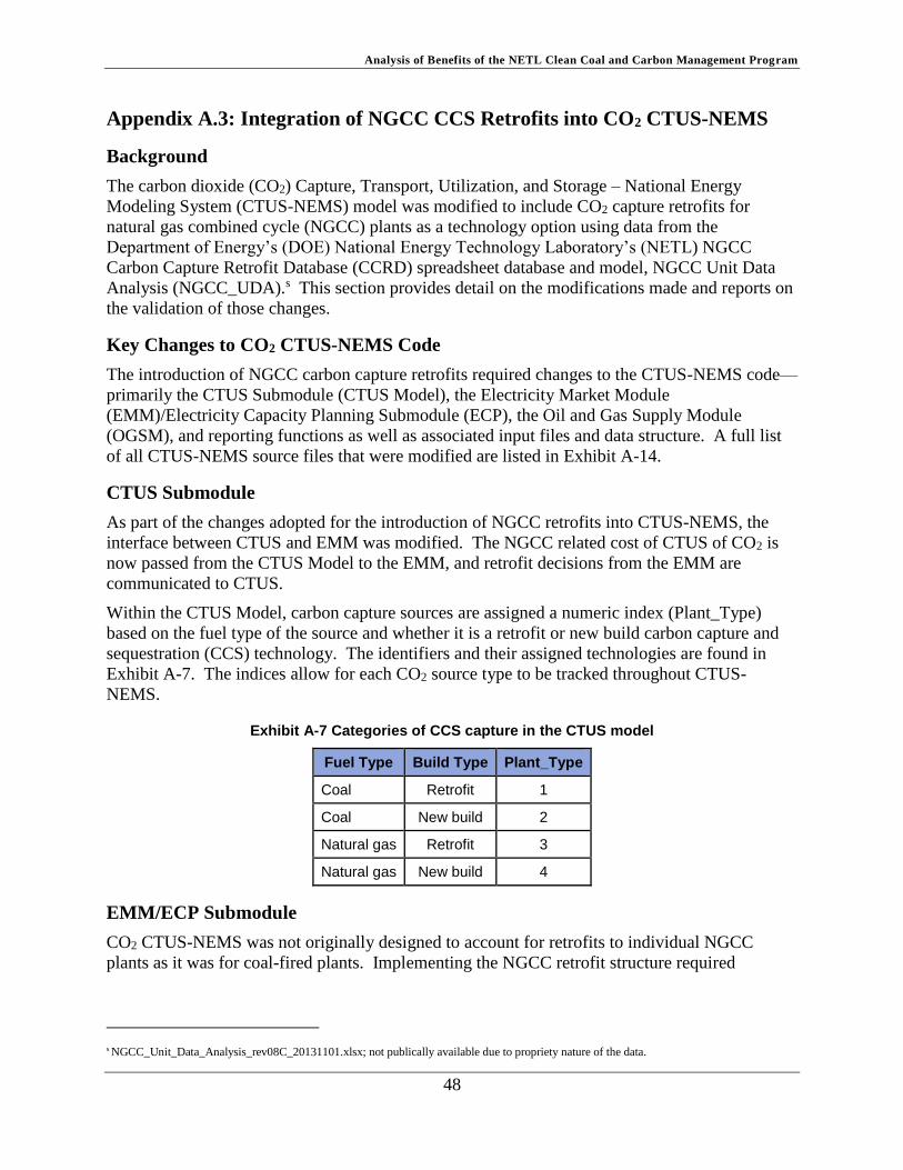
Analysis of Benefits of the NETL Clean Coal and Carbon Management Program
48
Appendix A.3: Integration of NGCC CCS Retrofits into CO2 CTUS-NEMS
Background
The carbon dioxide (CO2) Capture, Transport, Utilization, and Storage – National Energy
Modeling System (CTUS-NEMS) model was modified to include CO2 capture retrofits for
natural gas combined cycle (NGCC) plants as a technology option using data from the
Department of Energy’s (DOE) National Energy Technology Laboratory’s (NETL) NGCC
Carbon Capture Retrofit Database (CCRD) spreadsheet database and model, NGCC Unit Data
Analysis (NGCC_UDA).s This section provides detail on the modifications made and reports on
the validation of those changes.
Key Changes to CO2 CTUS-NEMS Code
The introduction of NGCC carbon capture retrofits required changes to the CTUS-NEMS code—
primarily the CTUS Submodule (CTUS Model), the Electricity Market Module
(EMM)/Electricity Capacity Planning Submodule (ECP), the Oil and Gas Supply Module
(OGSM), and reporting functions as well as associated input files and data structure. A full list
of all CTUS-NEMS source files that were modified are listed in Exhibit A-14.
CTUS Submodule
As part of the changes adopted for the introduction of NGCC retrofits into CTUS-NEMS, the
interface between CTUS and EMM was modified. The NGCC related cost of CTUS of CO2 is
now passed from the CTUS Model to the EMM, and retrofit decisions from the EMM are
communicated to CTUS.
Within the CTUS Model, carbon capture sources are assigned a numeric index (Plant_Type)
based on the fuel type of the source and whether it is a retrofit or new build carbon capture and
sequestration (CCS) technology. The identifiers and their assigned technologies are found in
Exhibit A-7. The indices allow for each CO2 source type to be tracked throughout CTUS-
NEMS.
Exhibit A-7 Categories of CCS capture in the CTUS model
Fuel Type Build Type Plant_Type
Coal Retrofit 1
Coal New build 2
Natural gas Retrofit 3
Natural gas New build 4
EMM/ECP Submodule
CO2 CTUS-NEMS was not originally designed to account for retrofits to individual NGCC
plants as it was for coal-fired plants. Implementing the NGCC retrofit structure required
s NGCC_Unit_Data_Analysis_rev08C_20131101.xlsx; not publically available due to propriety nature of the data.
Analysis of Benefits of the NETL Clean Coal and Carbon Management Program
49
eliminating the original treatment of NGCC and introducing a new plant type and associated new
data structure. Within the EMM, a new sub-routine (EPO$NGCC) was introduced in the ECP
Submodule to allow individual existing NGCC units a full range of possible actions which
include:
● Continue to use unit in all ECP planning periodst without retrofit
● Use unit as is in current period and then retrofit with capture for final two ECP periods
● Use unit as is in the first two ECP periods and then retrofit with capture for the final ECP
period
● Once retrofitted, allow the unit to operate with carbon capture for all three ECP periods
A second sub-routine was created in ECP to capture the NGCC retrofit decisions of existing
units. Finally, an existing ECP sub-routine was modified, allowing the appropriate linear
programming structure to be created for must-run and non-must-run units in each region that
have or could have retrofitted NGCC units.
Changes were also made to the Electricity Fuel Dispatch Submodule (EFD) to account for CO2
from retrofitted NGCC units.
OGSM
OGSM was modified to accept the new NGCC retrofits as sources of CO2 for enhanced oil
recovery (EOR) or for storage in saline structures (CO2 captured from coal plants was already
being accounted for in OGSM). CO2 captured from both NGCC and coal-fired plants and used
for EOR was combined in a single “Power Plants” category in OGSM. Routines which pass CO2
information between the submodules of CTUS-NEMS were also modified to properly account
for CO2 from NGCC retrofits.
Reporting
New reporting variables were created and added to the restart dictionary file, and the “FTAB”
code and input files were modified to include the new ECP plant type and to report separately the
NGCC retrofits capacity and generation.
Data Preparation
The NGCC carbon capture and retrofit data used in CTUS-NEMS was derived from NETL’s
NGCC_UDA. The data provided by NETL was aggregated at a higher level than that used in
CTUS-NEMS (which is at the component/turbine level). This inconsistency prevented the direct
adoption of the NETL NGCC retrofit capital costs into CTUS-NEMS and required a simple
mapping of costs on a unitized (dollar per kW [2011$/kW]) basis to resolve the issue.
The mapping of capital costs followed a simple, three step process:
t The ECP has a three-period planning horizon to examine costs over a 30-year period. The first period is the current year when decisions are made
to initiate investment decisions; the second is the following year; and the third considers the accumulated costs for the final 28 years of the cost recovery period. The model uses multi-year optimization as it solves all the years simultaneously.
Analysis of Benefits of the NETL Clean Coal and Carbon Management Program
50
1. For each unit in the NETL NGCC_UDA, a 2011$/kW cost was derived by dividing the
“Total CO2 Capture Retrofit CAPEX (total overnight cost [TOC] Basis)” by the “Pre-
Retrofit Total Capacity.”
2. The units in the NETL NGCC _UDA were mapped to the corresponding components in
the CO2 CTUS-NEMS database using plant and unit codes.
3. The 2011$/kW figure derived from the NETL data was multiplied by the summer
capacity of the corresponding components in the CTUS-NEMS data (from the pltf860
file) to allocate the capital cost associated over the units in the plant.
Within CTUS-NEMS, the plant units are aggregated back to the plant level and stored in the
RetroBase variable in the CTSinput.gdx database. Variable costs are stored, by plant, in the
CapCostVar variable of the CTSinput.gdx database. The component capital costs are aggregated
to a total plant capital cost within the standard structure of NEMS.
Variable costs for NGCC CCS retrofits are derived from the incremental operating cost
components in NGCC_UDA and include fixed labor, fixed taxes, and insurance and variable
costsu and are given on a dollar per short ton (2011$/ton) basis. For use in CTUS-NEMS, the
figures are adjusted for an assumed 75 percent capacity factor and converted to dollars per tonne
(2011$/tonne).
Financial Treatment of the Capital Investments
Previous versions of CTUS-NEMS calculated and transferred an annual annuity of capital costs
from the CTUS Model to the EMM. As part of the work under 342.04.05, Sub-Activity 2, this
methodology was changed so capital costs for both NGCC retrofits and coal retrofits are now
transferred from the CTUS submodule to the EMM as overnight capital costs. All financial
treatment of the overnight capital costs is performed within the existing construct of NEMS.
This change ensures consistency in financial treatment of power plant capital investments across
technologies in the EMM.
Crosswalk and Validation
The crosswalk and validation of the NGCC CCS retrofit costs each provide a different service in
the verification process. The crosswalk provides a direct mapping of NETL NGCC CCS retrofit
costs to their counterparts in CTUS-NEMS, while the validation confirms that the results from a
CTUS-NEMS model confirm functionality of the model modifications.
Crosswalk
The purpose of the crosswalk is to provide a mapping of the original NETL cost figures for
NGCC CCS retrofits to their representation in CTUS-NEMS. Following the steps outlined in the
Data Preparation section above, the path of a NGCC retrofit can be traced from the
NGCC_UDA to the RetroBase input variable in CTUS-NEMS. Tracing the input cost
assumption to the unit cost figures (namely, “Unit_Capture_Costs-Fixed” and
“Unit_Capture_Costs-Variable”) in the CTUS-NEMS output reporting (CTSSoln.gdx), requires
u Variable costs were calculated assuming a 100% capacity factor.

Analysis of Benefits of the NETL Clean Coal and Carbon Management Program
51
several more steps that occur in the reporting submodule (ctsreprt.gms). The unit cost
calculation is the same for coal retrofit costs and NGCC retrofit costs and is shown in Exhibit
A-6.
Crosswalk to Cost Inputs
The Cape Canaveral Power Plant (Energy Information Administration [EIA] Plant Identification
Number: 609) is an NGCC power plant and will be used to illustrate the crosswalk. The capital
costs of the CCS retrofit and the capacity of the plant recorded in NETL’s NGCC_UDA are
$1,012 million and 1,219 MW, respectively. Following the three data preparation steps (listed in
the Data Preparation section above), the capital cost input variable in CTUS-NEMS, RetroBase,
is calculated:
1. The capacity is divided by the cost to calculate a unitized cost value (2011$/kW):
a. $1,012 million / 1,219 MW = $830.42/kW
2. Plant 609 is comprised of four units in the CTUS-NEMS plant database, each with its
own capacity (Exhibit A-8).
3. The capacity of each generating unit of plant 609 is multiplied by the unitized cost figure
to calculate the capital cost of the NGCC retrofit (Exhibit A-8).
Exhibit A-8 Plant 609 capital cost by generating unit in CTUS-NEMS plant database
Plant 609 Unit Capacity (MW) Cost (2011$/kW) Capital Cost
(million$)
3A 247.6 830.42 205.6
3B 247.6 830.42 205.6
3C 247.6 830.42 205.6
3ST 467.2 830.42 388.0
Total plant 1,210 830.42 1,005
Within CTUS-NEMS, the per unit capital costs are aggregated into the RetroBase variable. The
discrepancy in the capital cost between the NGCC_UDA and CTUS-NEMS is due to the slight
(<1%) difference in the capacity of the plant between the two models.
The incremental operating expenses in NGCC_UDA for plant 609 total $9.41/ton (2011$) based
on 100 percent capacity factor. Adjusting for capacity factor and converting to tonnes, the value
used in CTUS-NEMS becomes $7.76 (2011$) using the equation:
CapCostVar = VarCost * CF * tonneConv (eq. 1)
Where:
CapCostVar = CTUS-NEMS input for variable cost (2011$/tonne)
VarCost = NGC_UDA variable cost (2012$/ton)
CF = capacity factor = 0.75
tonneConv = conversion factor from tons to tonnes = 1.1 ton/tonne
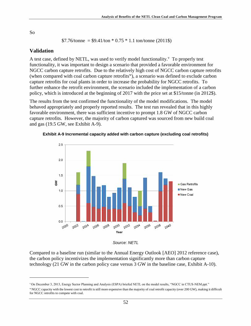
Analysis of Benefits of the NETL Clean Coal and Carbon Management Program
52
So
$7.76/tonne = $9.41/ton * 0.75 * 1.1 ton/tonne (2011$)
Validation
A test case, defined by NETL, was used to verify model functionality.v To properly test
functionality, it was important to design a scenario that provided a favorable environment for
NGCC carbon capture retrofits. Due to the relatively high cost of NGCC carbon capture retrofits
(when compared with coal carbon capture retrofitsw), a scenario was defined to exclude carbon
capture retrofits for coal plants in order to increase the probability for NGCC retrofits. To
further enhance the retrofit environment, the scenario included the implementation of a carbon
policy, which is introduced at the beginning of 2017 with the price set at $15/tonne (in 2012$).
The results from the test confirmed the functionality of the model modifications. The model
behaved appropriately and properly reported results. The test run revealed that in this highly
favorable environment, there was sufficient incentive to prompt 1.8 GW of NGCC carbon
capture retrofits. However, the majority of carbon captured was sourced from new build coal
and gas (19.5 GW, see Exhibit A-9).
Exhibit A-9 Incremental capacity added with carbon capture (excluding coal retrofits)
Source: NETL
Compared to a baseline run (similar to the Annual Energy Outlook [AEO] 2012 reference case),
the carbon policy incentivizes the implementation significantly more than carbon capture
technology (21 GW in the carbon policy case versus 3 GW in the baseline case, Exhibit A-10).
v On December 3, 2013, Energy Sector Planning and Analysis (ESPA) briefed NETL on the model results, “NGCC in CTUS-NEM.ppt.”
w NGCC capacity with the lowest cost to retrofit is still more expensive than the majority of coal retrofit capacity (over 200 GW), making it difficult for NGCC retrofits to compete with coal.

Analysis of Benefits of the NETL Clean Coal and Carbon Management Program
53
As would be expected, the volume of CO2 captured corresponds with the capacity values
(Exhibit A-11).
Exhibit A-10 Capacity with CO2 capture by technology type
Source: NETL
Exhibit A-11 Volume of CO2 captured from power plants over time
Source: NETL
The carbon captured from power plants shifts the sourcing ratio for CO2 used in EOR away from
natural and industrial sources and towards power plants. In the baseline scenario, only 6 percent
of the CO2 was sourced from power plants versus 35 percent in the carbon policy case (Exhibit

Analysis of Benefits of the NETL Clean Coal and Carbon Management Program
54
A-12). The increase in EOR activity between the baseline and the scenario is a result of the
influence of the carbon policy (Exhibit A-13). Additional CO2 captured from power plants is
sequestered in saline storage.
Exhibit A-12 Sources of CO2 for EOR
Source: NETL
Exhibit A-13 EOR activity
Source: NETL
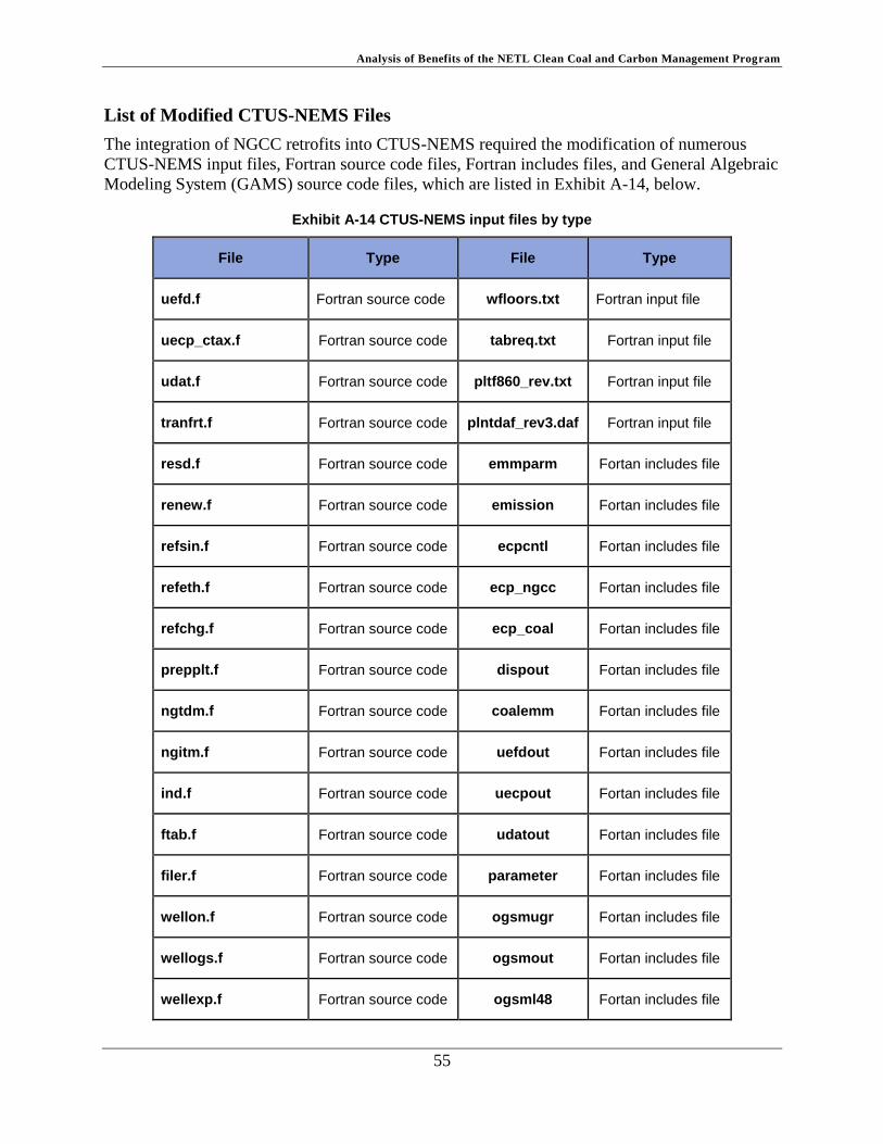
Analysis of Benefits of the NETL Clean Coal and Carbon Management Program
55
List of Modified CTUS-NEMS Files
The integration of NGCC retrofits into CTUS-NEMS required the modification of numerous
CTUS-NEMS input files, Fortran source code files, Fortran includes files, and General Algebraic
Modeling System (GAMS) source code files, which are listed in Exhibit A-14, below.
Exhibit A-14 CTUS-NEMS input files by type
File Type File Type
uefd.f Fortran source code wfloors.txt Fortran input file
uecp_ctax.f Fortran source code tabreq.txt Fortran input file
udat.f Fortran source code pltf860_rev.txt Fortran input file
tranfrt.f Fortran source code plntdaf_rev3.daf Fortran input file
resd.f Fortran source code emmparm Fortan includes file
renew.f Fortran source code emission Fortan includes file
refsin.f Fortran source code ecpcntl Fortan includes file
refeth.f Fortran source code ecp_ngcc Fortan includes file
refchg.f Fortran source code ecp_coal Fortan includes file
prepplt.f Fortran source code dispout Fortan includes file
ngtdm.f Fortran source code coalemm Fortan includes file
ngitm.f Fortran source code uefdout Fortan includes file
ind.f Fortran source code uecpout Fortan includes file
ftab.f Fortran source code udatout Fortan includes file
filer.f Fortran source code parameter Fortan includes file
wellon.f Fortran source code ogsmugr Fortan includes file
wellogs.f Fortran source code ogsmout Fortan includes file
wellexp.f Fortran source code ogsml48 Fortan includes file

Analysis of Benefits of the NETL Clean Coal and Carbon Management Program
56
File Type File Type
welleor.f Fortran source code ogsmeor Fortan includes file
wellcost.f Fortran source code ogglobal Fortan includes file
util.f Fortran source code ftable Fortan includes file
uefp_p.f Fortran source code fdict Fortan includes file
mnrisk.tax.txt Fortran input file enewtech Fortan includes file
layout.txt Fortran input file ctsprep.gms GAMS code file
epmdata.ctax15.txt Fortran input file ctsmodel.gms GAMS code file
epmcntl.ctax.15.txt Fortran input file ctsshell.gms GAMS code file
eintlrn.txt Fortran input file ctsreprt.gms GAMS code file
expdat.txt Fortran input file CTSinput.gdx GAMS code file
dict_new.txt Fortran input file CTSSoln.gdx GAMS output file
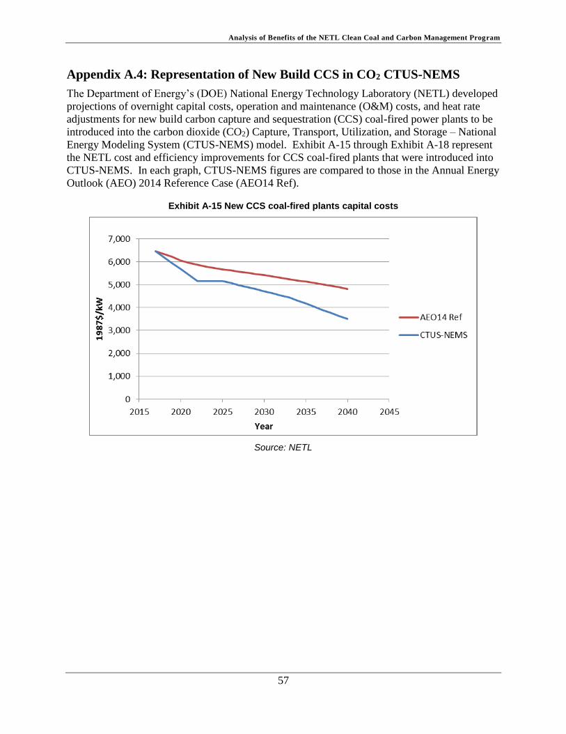
Analysis of Benefits of the NETL Clean Coal and Carbon Management Program
57
Appendix A.4: Representation of New Build CCS in CO2 CTUS-NEMS
The Department of Energy’s (DOE) National Energy Technology Laboratory (NETL) developed
projections of overnight capital costs, operation and maintenance (O&M) costs, and heat rate
adjustments for new build carbon capture and sequestration (CCS) coal-fired power plants to be
introduced into the carbon dioxide (CO2) Capture, Transport, Utilization, and Storage – National
Energy Modeling System (CTUS-NEMS) model. Exhibit A-15 through Exhibit A-18 represent
the NETL cost and efficiency improvements for CCS coal-fired plants that were introduced into
CTUS-NEMS. In each graph, CTUS-NEMS figures are compared to those in the Annual Energy
Outlook (AEO) 2014 Reference Case (AEO14 Ref).
Exhibit A-15 New CCS coal-fired plants capital costs
Source: NETL
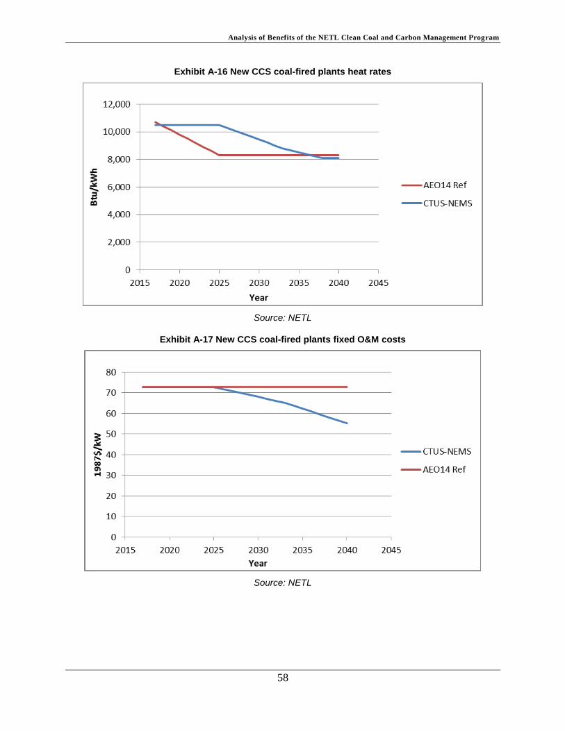
Analysis of Benefits of the NETL Clean Coal and Carbon Management Program
58
Exhibit A-16 New CCS coal-fired plants heat rates
Source: NETL
Exhibit A-17 New CCS coal-fired plants fixed O&M costs
Source: NETL

Analysis of Benefits of the NETL Clean Coal and Carbon Management Program
59
Exhibit A-18 New CCS coal-fired plants variable O&M costs
Source: NETL
These costs are incorporated into CTUS-NEMS through the existing process used in the Energy
Information Administration’s (EIA) NEMS model. Specifically, new build overnight capital and
O&M costs are entered in the ecpdat.txt input file. Using the corresponding Electricity Capacity
Planning Submodule (ECP) plant codes (35 or “IS” for new coal integrated gasification
combined cycle [IGCC] plantsx), the schedule of costs for each model year (2012 – 2040) is
entered in dollars per kilowatt (1987$/kW). Overnight capital costs use the UPOVCC variable,
while O&M costs use the UPOVFX variable to overwrite the default assumptions. All financial
treatment of the overnight capital costs is performed within the existing construct of NEMS.
This change ensures consistency in financial treatment of power plant capital investments across
technologies in the Electricity Market Module (EMM).
Heat rate adjustments are made through the unitless UCL_CF1 variable (used to calculate the
capacity loss variable, “CLOSS”) found in the emmcntrl.txt input file.
Validation of the incorporation of NETL cost figures for new builds into CTUS-NEMS is made
via visual inspection of the input files.
x The numeric technology indices are only applicable to the CTUS-NEMS version of the model based on the AEO14. This index can potentially change in different versions or releases of NEMS or CTUS-NEMS.

Analysis of Benefits of the NETL Clean Coal and Carbon Management Program
60
Appendix A.5: Enhanced Representation of Industrial Sources in CO2 CTUS-
NEMS
Background
Originally, in the carbon dioxide (CO2) Capture, Transport, Utilization, and Storage – National
Energy Modeling System (CTUS-NEMS) model, the price of collecting CO2 from an industrial
source in NEMS was assumed to be fixed for each industrial source type. In this enhanced
representation, sources of industrial CO2 are represented with supply curves which were
constructed based on cost and performance data developed by the Department of Energy’s
(DOE) National Energy Technology Laboratory (NETL).
NETL developed data that represent the expected cost of capture of CO2 and the potential
quantities available for capture from five industrial domestic sources: ammonia, cement,
ethanol, hydrogen refineries, and natural gas processing (NGP). NETL sought to use this data to
develop CO2 supply curves which would replace the industrial source data used by the Energy
Information Administration (EIA) in NEMS and CTUS-NEMS. The modifications leverage the
existing NEMS model structure enabling an efficient transition from static pricing to the supply
curve method.
Methodology
Developing the industrial CO2 supply curves and implementing them into the NEMS framework
involved several steps including:
● Preparation of the NETL data to work within the NEMS structure
● Modifying the CTUS-NEMS code to read in the NETL data
● Modifying the CTUS-NEMS code to use a supply curve approach for industrial CO2
rather than the existing approach, which uses static prices and volumes by industrial CO2
source
Data Preparation
The NETL industrial source dataset contains prices and volumes of CO2 by industrial source type
(NGP, ethanol, ammonia, cement, and hydrogen processing) and location (state) by facility.y To
prepare the raw NETL data for use in the CTUS-NEMS framework, it was first organized into
the seven regions used by the NEMS Oil and Gas Supply Module (OGSM): Northeast, Gulf
Coast, Midcontinent, Southwest, Rocky Mountain, Northern Great Plains, and West Coast
(Exhibit A-19). Next, NEMS used technology adoption rates and market penetration rates to
determine the time frame over which sources of industrial CO2 will be available. When
combined, these technology adoption and market penetration rates created availability curves
which represented the percent of total CO2 available in a given year by industrial source type
(Exhibit A-20). These curves were applied to the NETL data, resulting in time-dependent CO2
availability curves for CO2 volumes by region and source type.
y NETL file: “Results_Summary.xlsx,” dated January 6, 2104.

Analysis of Benefits of the NETL Clean Coal and Carbon Management Program
61
Exhibit A-19 Seven OGSM regions in NEMS
Source: EIA
Exhibit A-20 Industrial CO2 availability curve in NEMS
Source: NETL

Analysis of Benefits of the NETL Clean Coal and Carbon Management Program
62
Representing Supply Curves in NEMS
Based on the data in the industrial CO2 analysis, NETL developed a supply curve for industrial
CO2 sources (Exhibit A-21). This curve represents price (P) and quantity (Q) pairs across all
industrial sources, independent of time.z In order to be used in NEMS, this supply curve was
transformed into regional, time-dependent supply curves.
Exhibit A-21 NETL industrial CO2 time independent supply curve
Source: NETL
To do this, the P and Q pairs were combined with the location data from NETL to first create
regional time independent supply curves. The availability curves (see Exhibit A-20) were then
applied to the regional supply curves to produce a set of time-dependent supply curves for each
region that phases in the CO2 availability annually across the model’s time horizon (Exhibit
A-22).
The default NEMS representation of industrial sources of CO2 had eight positions organized by
industrial source that could be re-purposed to create a supply curve.aa To create supply curves
z From NETL file: Results_Summary.xls dated January 7, 2014.
aa Other approaches to implementation were considered but rejected on the grounds that they would entail extensive modification to the Electricity
Market Module (EMM) (and in the 2014 version of NEMS, Liquid Fuels Market Module) that was well beyond the resources available and would not contribute materially to improving the modeling.

Analysis of Benefits of the NETL Clean Coal and Carbon Management Program
63
within the NEMS framework, sources with similar prices (regardless of industrial source) were
assigned a single price which represents the quantity of CO2 that is available at that price. The
price points were selected so that the highest price within the group’s range could be used to
represent quantity in the bin. Eight of these “price bins” were used to capture the range of prices
in the dataset. The boundary prices used to characterize the price/quantity bins are a model input
and can be changed at the discretion of the user to best represent the underlying data. As
currently modeled, the following price bins were used (in dollars per tonne [2011$/tonne]): $35,
$40, $43, $47, $50, $53, $70, and $150, and represent the lower price bound for each bin. At the
lower end of the price spectrum, where greater competition is expected, the range between the
price bins is narrow, allowing for more price differentiation. At the higher end of the scale,
where the prices are not expected to be competitive, the range between price bins is greater.
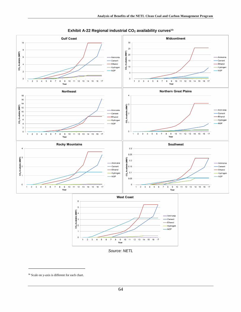
Analysis of Benefits of the NETL Clean Coal and Carbon Management Program
64
Exhibit A-22 Regional industrial CO2 availability curvesbb
Source: NETL
bb Scale on y-axis is different for each chart.

Analysis of Benefits of the NETL Clean Coal and Carbon Management Program
65
The default NEMS representation of industrial CO2 sources consists of eight positions (one CO2
source for each position). These positions were re-purposed into price bins used to create
regional industrial CO2 supply curves.cc Each of the eight positions in the NEMS framework
was assigned a boundary price that represented the price that would be received for any quantity
of CO2 coming from an industrial source assigned to that price bin. The boundary prices were
determined by first ranking all industrial CO2 sources by prices and assigning sources with
similar prices to the same price bin. The highest price within the group assigned to the same
price bin was used as the boundary price. The boundary prices were determined by examining
the industrial CO2 price distribution (Exhibit A-23) and determining where there were price
concentrations. At the lower end of the price spectrum, where greater competition is expected, a
narrow range between the price bins was set, allowing for more price differentiation. At the
higher end of the scale, where the prices are not expected to be competitive, the range between
price bins was made larger. The boundary prices used to characterize the price/quantity bins are
a model input and can be changed by modifying the pq_bins_regional_rev4.xml input file, at the
discretion of the user to best represent the underlying data. As currently modeled, the following
price bins are used (in 2011$/tonne): $35, $40, $43, $47, $50, $53, $70, and $150.
Exhibit A-23 Industrial CO2 price distribution
Source: NETL
Using an example from the Midcontinent region (one of the more active supply regions), Exhibit
A-24 provides a comparison between the supply curves as created from NETL and the
cc Other approaches to implementation were considered but rejected on the grounds that they would entail extensive modification to the EMM that was well beyond the resources available and would not contribute materially to improving the modeling.

Analysis of Benefits of the NETL Clean Coal and Carbon Management Program
66
translation of the supply curves using the “price bin” approach to accommodate NEMS’s
existing framework. The top row of graphs represents the time phased availability of CO2 by
industrial source before applying the bin aggregation. The bottom row of graphs represents this
same data after the bins have been formed.
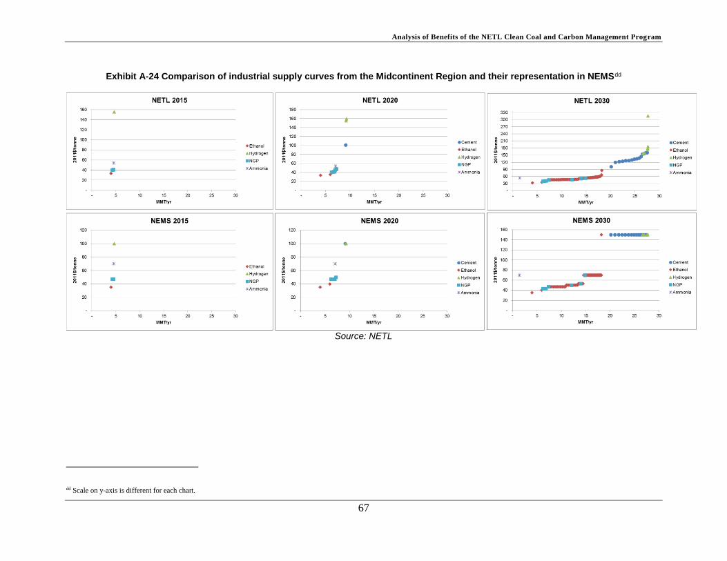
Analysis of Benefits of the NETL Clean Coal and Carbon Management Program
67
Exhibit A-24 Comparison of industrial supply curves from the Midcontinent Region and their representation in NEMSdd
Source: NETL
dd Scale on y-axis is different for each chart.
Analysis of Benefits of the NETL Clean Coal and Carbon Management Program
68
Source Code Modifications
The OGSM in NEMS was modified to accommodate the NETL data and the supply curve
approach to industrial CO2 sources. Modifications were made to the accounting of CO2 in
OGSM to allow proper flow through of OGSM evaluation and selection mechanisms and to
ensure accurate reporting of the model output.
For accounting purposes, CO2 is organized both by price bins and industrial source type. A total
of four arrays are needed to hold price and volume data. Two new restart arrays were created to
hold available and purchased CO2, organized by industrial source type. The original arrays store
available and purchased CO2 by price bins.
Within the NEMS code the following modifications were made to the OGSM submodules:
WELLOGS.f was modified to account for the new arrays
WELLCOST.f was modified to strip transport cost from industrial capture cost and store
CO2 prices by year. Transport cost is later added back to capture costs. The amount of
the transport cost varies depending upon the ultimate path taken by the CO2
WELLON.f was modified to read in NETL industrial CO2 availability by source type
o Each industrial CO2 source is assigned a start year (based on existing EIA
assumptions)
o Regional CO2 volumes over time are tracked separately by source type and by price
bin
o OGSM first uses the array sorted by price bin to determine the amount of CO2
purchased
o CO2 amounts determined in the first (price bin) sorting process are then resorted by
source type and OGSM region. This is done so that CO2 purchases can be properly
reported by source type
The following modification was made to reporting:
FTAB.f was changed to use the new arrays for “Available Carbon Dioxide” and
“Purchased Carbon Dioxide,” sorted by industry type in Table 25 (note: other arrays used
in Table 25 namely, “Recycled Carbon Dioxide,” “Carbon Dioxide Used,” and “Oil
Produced (by source),” are not comparable to “Available Carbon Dioxide” and
“Purchased Carbon Dioxide”)
Functionality Verification
The functionality of the changes made to CTUS-NEMS to employ supply curves for industrial
CO2 sources was verified by running a $15 carbon price case. Due to the generally higher cost
of CO2 and lower volumes available, industrially sourced CO2 is not a dominant player in the
market for purchased CO2 (Exhibit A-25). Only the lowest priced industrial sources (NGP and
ethanol) can compete with power plants in a carbon price scenario.

Analysis of Benefits of the NETL Clean Coal and Carbon Management Program
69
Exhibit A-25 CO2 purchased for EOR production
Source: NETL
0
10
20
30
40
50
60
70
80
90
100
2015 2020 2025 2030 2040
MM
T
Year
Natural
NGP
Ethanol
Power Plants
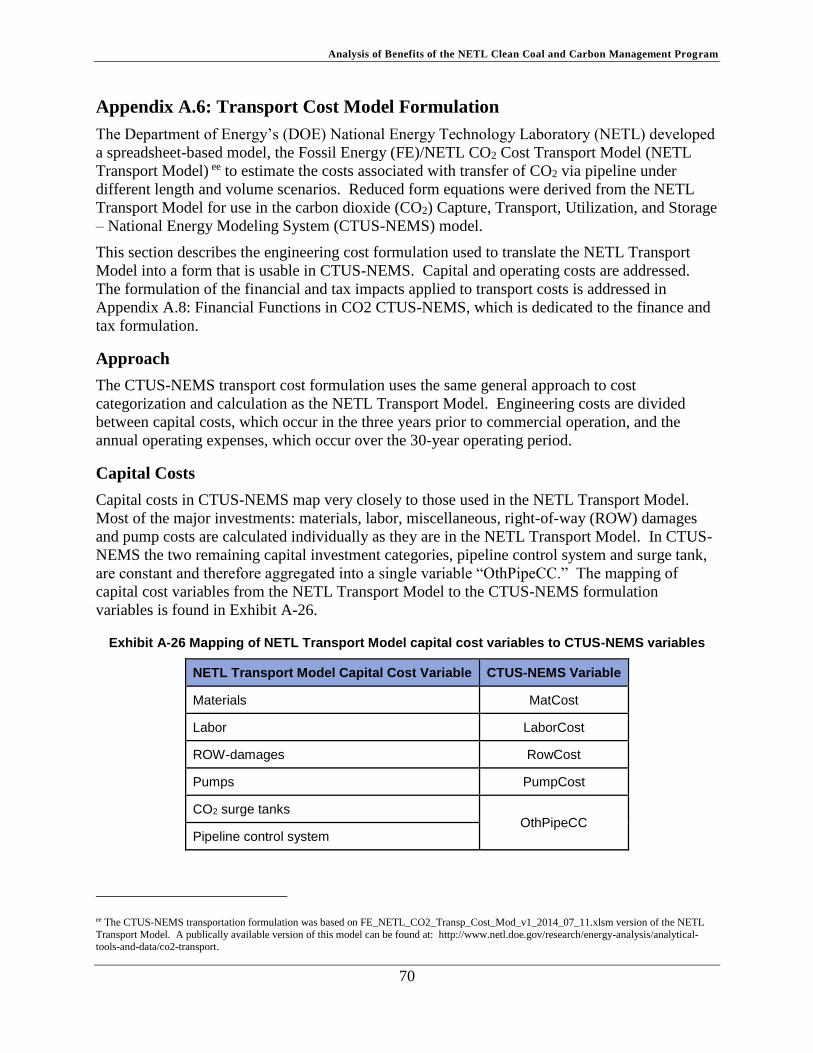
Analysis of Benefits of the NETL Clean Coal and Carbon Management Program
70
Appendix A.6: Transport Cost Model Formulation
The Department of Energy’s (DOE) National Energy Technology Laboratory (NETL) developed
a spreadsheet-based model, the Fossil Energy (FE)/NETL CO2 Cost Transport Model (NETL
Transport Model) ee to estimate the costs associated with transfer of CO2 via pipeline under
different length and volume scenarios. Reduced form equations were derived from the NETL
Transport Model for use in the carbon dioxide (CO2) Capture, Transport, Utilization, and Storage
– National Energy Modeling System (CTUS-NEMS) model.
This section describes the engineering cost formulation used to translate the NETL Transport
Model into a form that is usable in CTUS-NEMS. Capital and operating costs are addressed.
The formulation of the financial and tax impacts applied to transport costs is addressed in
Appendix A.8: Financial Functions in CO2 CTUS-NEMS, which is dedicated to the finance and
tax formulation.
Approach
The CTUS-NEMS transport cost formulation uses the same general approach to cost
categorization and calculation as the NETL Transport Model. Engineering costs are divided
between capital costs, which occur in the three years prior to commercial operation, and the
annual operating expenses, which occur over the 30-year operating period.
Capital Costs
Capital costs in CTUS-NEMS map very closely to those used in the NETL Transport Model.
Most of the major investments: materials, labor, miscellaneous, right-of-way (ROW) damages
and pump costs are calculated individually as they are in the NETL Transport Model. In CTUS-
NEMS the two remaining capital investment categories, pipeline control system and surge tank,
are constant and therefore aggregated into a single variable “OthPipeCC.” The mapping of
capital cost variables from the NETL Transport Model to the CTUS-NEMS formulation
variables is found in Exhibit A-26.
Exhibit A-26 Mapping of NETL Transport Model capital cost variables to CTUS-NEMS variables
NETL Transport Model Capital Cost Variable CTUS-NEMS Variable
Materials MatCost
Labor LaborCost
ROW-damages RowCost
Pumps PumpCost
CO2 surge tanks OthPipeCC
Pipeline control system
ee The CTUS-NEMS transportation formulation was based on FE_NETL_CO2_Transp_Cost_Mod_v1_2014_07_11.xlsm version of the NETL
Transport Model. A publically available version of this model can be found at: http://www.netl.doe.gov/research/energy-analysis/analytical-tools-and-data/co2-transport.
Analysis of Benefits of the NETL Clean Coal and Carbon Management Program
71
Capital Cost Formulation
The NETL Transport Model allows the user to select from a variety of methods to calculate
pipeline capital costs. The Parker method was used in the formulation of the material, labor,
ROW, and miscellaneous equations used in CTUS-NEMS. The Parker method uses the
following form for each of its capital cost equations:
CCi = ai-0 + L * (ai-1 * D2 + ai-2 * D + ai-3) (eq. 1)
Where:
i = identifier for the cost category (m for materials, l for labor, r for
ROW and misc for miscellaneous)
CCi = capital cost for category i (2004$)
L = length of pipeline (mi)
D = standard diameter of pipeline (in)
ai-0, ai-1, ai-2, ai-3 = parameters determined by fitting the equation to capital cost data
In the CTUS-NEMS formulation, two additional parameters are included in the capital cost
equation to escalate the figures to 2011 dollars and another account for the price difference
between the pipe thickness of a natural gas pipeline (on which the Parker method equations were
estimated) and that of a CO2 pipeline. Thus, the generalized equation in CTUS-NEMS for
material, labor, ROW, and miscellaneous costs is:
CCi = ai-0 + L * (ai-1 * D2 + ai-2 * D + ai-3) * CO2esc * CO2adj (eq. 2)
Where:
i = identifier for the cost category (materials, labor, ROW, and misc
for miscellaneous)
CCi = capital cost for category i (2004$)
L = length of pipeline (mi)
D = standard diameter of pipeline (in)
ai-0, ai-1, ai-2, ai-3 = parameters determined by fitting the equation to capital cost data
CO2esc = variable-specific escalator that brings the equation (in 2000$) to
2011$
CO2adj = the coefficient that adjusts for the price difference in the pipe
thickness between natural gas and CO2 pipelines (unitless)
In CTUS-NEMS, the ai-0, ai-1, ai-2, ai-3 parameters are inputs which are stored in the Tcosts table
of the CTSinput.gdx file. These parameters are given different identifiers in CTUS-NEMS,
which can be found in Exhibit A-27.

Analysis of Benefits of the NETL Clean Coal and Carbon Management Program
72
Exhibit A-27 Mapping of Parker equation parameters to CTUS-NEMS parameter names
Parker Equation Parameter Names CTUS-NEMS Parameter Names
ai-0 Fixed
ai-1 DD
ai-2 D
ai-3 Constant
The remaining capital costs are for pumps and other pipeline capital costs (CO2 surge tanks and
pipeline control systems). The McCollum and Ogden cost estimate for pumps was used in the
CTUS-NEMS formulation. The capital cost for pumps is a function of the number of pumps and
the power required by a pump. Therefore, there is a unit pump cost (“UnitPump,”
2011$/pump)—an input to the model (stored in the Tcosts table)—which is multiplied by the
number of pumps (PumpNum) and a unit pump power cost (“PumpCapCC,” 2011$/MW)—also
an input to the model (stored in the Tcosts table)—which is multiplied by the pump power
requirement (P_Pwr). Together, these are combined to calculate the total pump capital cost:
PumpCost = PumpCapCC * P_Pwr + UnitPump * PumpNum (eq. 3)
Where:
PumpCost = engineering capital cost for the pumps on a pipeline (2011$)
PumpCapCC = unit pump power cost coefficient (2011$/MW)
P_Pwr = power requirement for the pumps (MW)
UnitPump = unit pump cost coefficient (2011$/pump)
PumpNum = number of pumps on the pipeline
The pump power requirement is a function of the pipe diameter, and the pump number is a
function of both the pipe diameter (in) and pipe length (mi). The power requirement is
calculated as
P_Pwr = Elec_Coeff * PipeMax / PipeCapacity / 1,000 (eq. 4)
Where:
P_Pwr = power requirement for the pumps (MW)
Elec_Coeff = constant coefficient that accounts for pump efficiency, the density of
CO2, and the total pressure change (MW/MMT)
PipeMax = maximum flow of a pipe (MMT/yr)
PipeCapacity = maximum usage percentage of a pipe (unitless)
The number of pumps required is dependent upon the diameter and length of the pipe. An input
table of number of pumps required, dimensioned by pipe diameter and length was created based
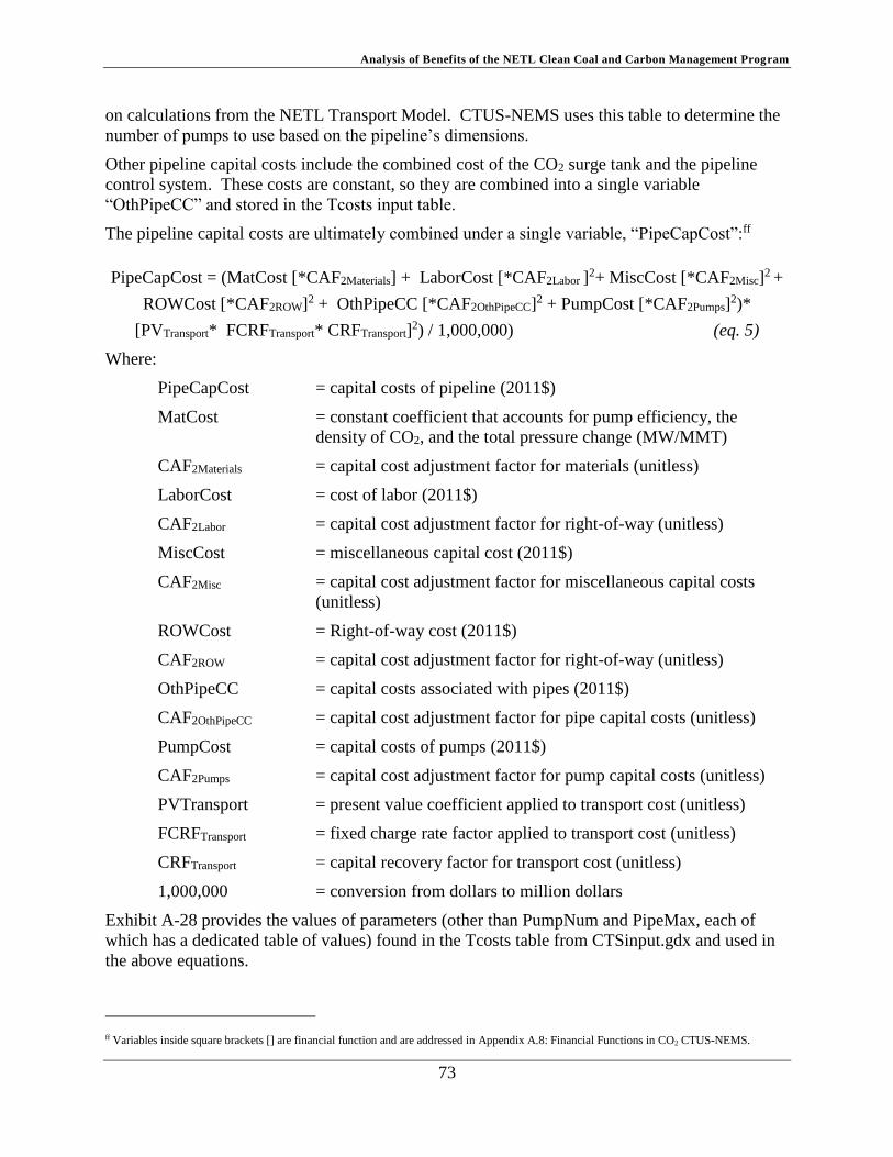
Analysis of Benefits of the NETL Clean Coal and Carbon Management Program
73
on calculations from the NETL Transport Model. CTUS-NEMS uses this table to determine the
number of pumps to use based on the pipeline’s dimensions.
Other pipeline capital costs include the combined cost of the CO2 surge tank and the pipeline
control system. These costs are constant, so they are combined into a single variable
“OthPipeCC” and stored in the Tcosts input table.
The pipeline capital costs are ultimately combined under a single variable, “PipeCapCost”:ff
PipeCapCost = (MatCost [*CAF2Materials] + LaborCost [*CAF2Labor ]2+ MiscCost [*CAF2Misc]
2 +
ROWCost [*CAF2ROW]2 + OthPipeCC [*CAF2OthPipeCC]2 + PumpCost [*CAF2Pumps]2)*
[PVTransport* FCRFTransport* CRFTransport]2) / 1,000,000) (eq. 5)
Where:
PipeCapCost = capital costs of pipeline (2011$)
MatCost = constant coefficient that accounts for pump efficiency, the
density of CO2, and the total pressure change (MW/MMT)
CAF2Materials = capital cost adjustment factor for materials (unitless)
LaborCost = cost of labor (2011$)
CAF2Labor = capital cost adjustment factor for right-of-way (unitless)
MiscCost = miscellaneous capital cost (2011$)
CAF2Misc = capital cost adjustment factor for miscellaneous capital costs
(unitless)
ROWCost = Right-of-way cost (2011$)
CAF2ROW = capital cost adjustment factor for right-of-way (unitless)
OthPipeCC = capital costs associated with pipes (2011$)
CAF2OthPipeCC = capital cost adjustment factor for pipe capital costs (unitless)
PumpCost = capital costs of pumps (2011$)
CAF2Pumps = capital cost adjustment factor for pump capital costs (unitless)
PVTransport = present value coefficient applied to transport cost (unitless)
FCRFTransport = fixed charge rate factor applied to transport cost (unitless)
CRFTransport = capital recovery factor for transport cost (unitless)
1,000,000 = conversion from dollars to million dollars
Exhibit A-28 provides the values of parameters (other than PumpNum and PipeMax, each of
which has a dedicated table of values) found in the Tcosts table from CTSinput.gdx and used in
the above equations.
ff Variables inside square brackets [] are financial function and are addressed in Appendix A.8: Financial Functions in CO2 CTUS-NEMS.

Analysis of Benefits of the NETL Clean Coal and Carbon Management Program
74
Exhibit A-28 Values for transportation capital cost input parameters in CTUS-NEMS
Cost Category
Fixed Length DD D Constant CO2esc
Materials 35,000 1 330.5 687 26,960 2.011
Labor 185,000 1 343.2 2,074 170,013 2.011
ROW 40,000 1 - 577 29,788 1.561
Misc 95,000 1 - 8,417 7,324 1.283
CO2Adj - - - - 1.12 -
UnitPump - - - - 83,581 -
PumpCapCC - - - - 1,325,362 -
Elec_Coeff - - - - 315.36 -
PipeCapacity - - - - 0.8 -
OthPipeCC - - - - 1,356,651 -
The capital costs are assumed to be incurred over three years prior to operations according to the
schedule in Exhibit A-29 (taken directly from the NETL Transport Model). The cost impact and
calculations during the pre-operational period is addressed separately in the financing
documentation.
Exhibit A-29 Distribution of capital costs during construction
Investment Item Year 1 Year 2 Year 3
Materials 5% 40% 55%
Labor 5% 40% 55%
ROW 55% 30% 15%
Misc 30% 35% 35%
OthPipeCC 30% 70%
Pumps 40% 60%
Operating and Maintenance Costs
Transportation operations and maintenance (O&M) costs in CTUS-NEMS are variable costs
dependent upon annual CO2 in the pipeline (dollars per tonne [2011$/tonne]) and consist of three
Analysis of Benefits of the NETL Clean Coal and Carbon Management Program
75
components: pipeline related equipment and pumps O&M (Equipment O&M), electricity costs
for pumps, and other pipeline O&M.
Equipment O&M or “PumpEquip” is represented as a fixed percentage (4.0 percent) of the
combined costs of pumps, the CO2 surge tank, and the pipeline control system:
PumpEquip = (PumpPC * (PumpCost + OthPipeCC)) (eq. 6)
Where:
PumpEquip = the annual O&M costs per million metric tonnes (MMT) of CO2
of pump and other pipeline related equipment (2011$)
PumpPC = the percentage of capital cost that represents annual O&M costs
(input, unitless)
PumpCost = the capital cost of the total number of pumps used on a pipeline
(2011$)
OthPipeCC = the capital cost of CO2 surge tanks and the pipeline control
system (2011$)
Pump electricity costs are calculated as a function of electricity required to operate a pump and
electricity price. Electricity required by the pump is represented as:
PumpElec = Elec_Coeff * PipeMax * 8,760*PumpNum / 1,000 (eq. 7)
Where:
PumpElec = electricity needed to run all necessary pumps (MWh/yr)
Elec_Coeff = coefficient to calculate amount of electricity needed for pump (input,
kW/MMT)
PipeMax = maximum flow of a pipe (input, MMT/yr)
8,760 = number of hours in one year
PumpNum = number of pumps required for pipeline
1,000 = conversion from kW to MW
Pump electricity costs (PumpElecCost) are therefore:
PumpElecCost = PumpElec * CompPwr_Price (eq. 8)
Where:
PumpElecCost = cost associated with electricity purchased to run pumps (2011$)
PumpElec = electricity needed to run all necessary pumps (MWh/yr)
CompPwr_Price = price of electricity (2011$/MWh from NEMS)
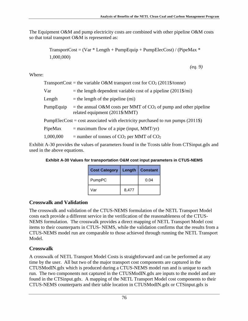
Analysis of Benefits of the NETL Clean Coal and Carbon Management Program
76
The Equipment O&M and pump electricity costs are combined with other pipeline O&M costs
so that total transport O&M is represented as:
TransportCost = (Var * Length + PumpEquip + PumpElecCost) / (PipeMax *
1,000,000)
(eq. 9)
Where:
TransportCost = the variable O&M transport cost for CO2 (2011$/tonne)
Var = the length dependent variable cost of a pipeline (2011$/mi)
Length = the length of the pipeline (mi)
PumpEquip = the annual O&M costs per MMT of CO2 of pump and other pipeline
related equipment (2011$/MMT)
PumpElecCost = cost associated with electricity purchased to run pumps (2011$)
PipeMax = maximum flow of a pipe (input, MMT/yr)
1,000,000 = number of tonnes of CO2 per MMT of CO2
Exhibit A-30 provides the values of parameters found in the Tcosts table from CTSinput.gdx and
used in the above equations.
Exhibit A-30 Values for transportation O&M cost input parameters in CTUS-NEMS
Cost Category Length Constant
PumpPC 0.04
Var 8,477
Crosswalk and Validation
The crosswalk and validation of the CTUS-NEMS formulation of the NETL Transport Model
costs each provide a different service in the verification of the reasonableness of the CTUS-
NEMS formulation. The crosswalk provides a direct mapping of NETL Transport Model cost
items to their counterparts in CTUS- NEMS, while the validation confirms that the results from a
CTUS-NEMS model run are comparable to those achieved through running the NETL Transport
Model.
Crosswalk
A crosswalk of NETL Transport Model Costs is straightforward and can be performed at any
time by the user. All but two of the major transport cost components are captured in the
CTUSModIN.gdx which is produced during a CTUS-NEMS model run and is unique to each
run. The two components not captured in the CTUSModIN.gdx are inputs to the model and are
found in the CTSinput.gdx. A mapping of the NETL Transport Model cost components to their
CTUS-NEMS counterparts and their table location in CTUSModIN.gdx or CTSinput.gdx is
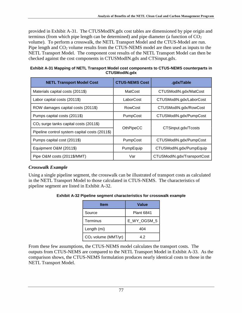
Analysis of Benefits of the NETL Clean Coal and Carbon Management Program
77
provided in Exhibit A-31. The CTUSModIN.gdx cost tables are dimensioned by pipe origin and
terminus (from which pipe length can be determined) and pipe diameter (a function of CO2
volume). To perform a crosswalk, the NETL Transport Model and the CTUS-Model are run.
Pipe length and CO2 volume results from the CTUS-NEMS model are then used as inputs to the
NETL Transport Model. The component cost results of the NETL Transport Model can then be
checked against the cost components in CTUSModIN.gdx and CTSinput.gdx.
Exhibit A-31 Mapping of NETL Transport Model cost components to CTUS-NEMS counterparts in CTUSModIN.gdx
NETL Transport Model Cost CTUS-NEMS Cost .gdx/Table
Materials capital costs (2011$) MatCost CTUSModIN.gdx/MatCost
Labor capital costs (2011$) LaborCost CTUSModIN.gdx/LaborCost
ROW damages capital costs (2011$) RowCost CTUSModIN.gdx/RowCost
Pumps capital costs (2011$) PumpCost CTUSModIN.gdx/PumpCost
CO2 surge tanks capital costs (2011$) OthPipeCC CTSinput.gdx/Tcosts
Pipeline control system capital costs (2011$)
Pumps capital cost (2011$) PumpCost CTUSModIN.gdx/PumpCost
Equipment O&M (2011$) PumpEquip CTUSModIN.gdx/PumpEquip
Pipe O&M costs (2011$/MMT) Var CTUSModIN.gdx/TransportCost
Crosswalk Example
Using a single pipeline segment, the crosswalk can be illustrated of transport costs as calculated
in the NETL Transport Model to those calculated in CTUS-NEMS. The characteristics of
pipeline segment are listed in Exhibit A-32.
Exhibit A-32 Pipeline segment characteristics for crosswalk example
Item Value
Source Plant 6841
Terminus E_WY_OGSM_5
Length (mi) 404
CO2 volume (MMT/yr) 4.2
From these few assumptions, the CTUS-NEMS model calculates the transport costs. The
outputs from CTUS-NEMS are compared to the NETL Transport Model in Exhibit A-33. As the
comparison shows, the CTUS-NEMS formulation produces nearly identical costs to those in the
NETL Transport Model.
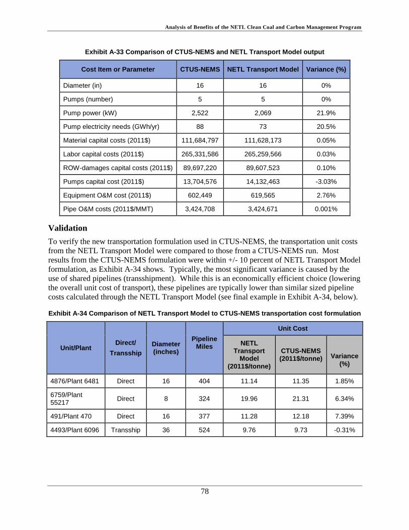
Analysis of Benefits of the NETL Clean Coal and Carbon Management Program
78
Exhibit A-33 Comparison of CTUS-NEMS and NETL Transport Model output
Cost Item or Parameter CTUS-NEMS NETL Transport Model Variance (%)
Diameter (in) 16 16 0%
Pumps (number) 5 5 0%
Pump power (kW) 2,522 2,069 21.9%
Pump electricity needs (GWh/yr) 88 73 20.5%
Material capital costs (2011$) 111,684,797 111,628,173 0.05%
Labor capital costs (2011$) 265,331,586 265,259,566 0.03%
ROW-damages capital costs (2011$) 89,697,220 89,607,523 0.10%
Pumps capital cost (2011$) 13,704,576 14,132,463 -3.03%
Equipment O&M cost (2011$) 602,449 619,565 2.76%
Pipe O&M costs (2011$/MMT) 3,424,708 3,424,671 0.001%
Validation
To verify the new transportation formulation used in CTUS-NEMS, the transportation unit costs
from the NETL Transport Model were compared to those from a CTUS-NEMS run. Most
results from the CTUS-NEMS formulation were within +/- 10 percent of NETL Transport Model
formulation, as Exhibit A-34 shows. Typically, the most significant variance is caused by the
use of shared pipelines (transshipment). While this is an economically efficient choice (lowering
the overall unit cost of transport), these pipelines are typically lower than similar sized pipeline
costs calculated through the NETL Transport Model (see final example in Exhibit A-34, below).
Exhibit A-34 Comparison of NETL Transport Model to CTUS-NEMS transportation cost formulation
Unit/Plant Direct/
Transship
Diameter (inches)
Pipeline Miles
Unit Cost
NETL Transport
Model (2011$/tonne)
CTUS-NEMS (2011$/tonne)
Variance (%)
4876/Plant 6481 Direct 16 404 11.14 11.35 1.85%
6759/Plant 55217
Direct 8 324 19.96 21.31 6.34%
491/Plant 470 Direct 16 377 11.28 12.18 7.39%
4493/Plant 6096 Transship 36 524 9.76 9.73 -0.31%

Analysis of Benefits of the NETL Clean Coal and Carbon Management Program
79
Appendix A.7: CO2 CTUS-NEMS Saline Cost Model Formulation
Background
The carbon dioxide (CO2) saline storage cost formulation in the CO2 Capture, Transport,
Utilization, and Storage – National Energy Modeling System (CTUS-NEMS) model was revised
to correspond with costs in the Fossil Energy (FE)/National Energy Technology Laboratory
(NETL) Saline Cost Model (NETL Saline Model).gg To achieve this, a set of parameterized
equations was developed that provide a reasonable representation of the saline storage costs from
the NETL Saline Model but which also accommodated the dynamics of the CTUS-NEMS
model. This section describes the engineering cost formulation used to translate the NETL
Saline Model into a form that is usable in NEMS. Capital and operating costs are addressed.
While the financial functions that are applied to the engineering costs appear in these equations
(inside brackets), their origin and function are not addressed here, but instead, addressed in
Appendix A.8: Financial Functions in CO2 CTUS-NEMS.
Throughout this section, units are provided for each variable. In the case that the variable is an
input, the name of the data table in which it is stored (within CTSinput.gdx) is provided. In
developing the formulation, the general structure was assumed for all formations as a way to
restrict the number of choices and reduce the amount of computational burden on the model.
Three distinct cost periods were defined to address specific financial characteristics of each
period:
Pre-operational period – the six-year period prior to commercial operation of the
storage site. All costs in this period are treated as capital investments
o Capital investment during the pre-operational period is distributed according to the
construction profile (Exhibit A-35)
Exhibit A-35 Pre-operational period capital investment: construction profile
Year 1 Year 2 Year 3 Year 4 Year 5 Year 6
1% 77% 5% 9% 1% 7%
Costs during the pre-operational period assume the maximum level of CO2 injection for
that site (based on the lesser of the nominal CO2 injection rate and the maximum plume
area).hh
Operational period - the 30-year period over which there is potential for or active CO2
injection into a saline formation. During the operational period, there are both recurring
capital investments and annual operations and maintenance (O&M) costs. The capital
investments are divided into two sets of recurring costs: five-year recurring capital costs
and three-year recurring capital costs. The five-year recurring capital costs are primarily
gg Model version: FE_NETL_CO2_Sal_Stor_Cost_Mod_ver_2.1_final_2014_07_18.xlsm is publically available at
http://www.netl.doe.gov/research/energy-analysis/analytical-tools-and-data/co2-saline-storage.
hh If capacity remains in the reservoir after the 100 square miles (mi2) radius constraint has been reached, the reservoir may still be used but will incur the “site cost” again.

Analysis of Benefits of the NETL Clean Coal and Carbon Management Program
80
costs associated with seismic testing activities, while the three-year capital costs account
for the remainder of capital costs that recur throughout the site’s operational life. While
not all saline storage sites have exactly the same recurring investment schedule, the five-
year/three-year schedule is a close approximation of the majority of them. The value of
the recurring investment for each category was calculated by dividing the summation of
the capital investments during operations by six or ten for five-year and three-year
investments, respectively
The annual O&M costs are categorized as either variable by the volume of CO2 injected
annually or by the number of injection wells per year
Post-Injection Site Care (PISC) period - The 50-year time period that begins
immediately after commercial operation, during which PISC and monitoring occurs.
Costs during this period are neither capital nor operating expenses. Instead, the model
formulation addresses the treatment of funds which must build up during the operational
phase and then be disbursed, as scheduled, over the post operational period
Ultimately, the formulation is organized around the dependencies of a function: well dependent;
tonnage dependent (CO2 injection), or independent which are represented by three equations:
Fixed new injection site costs (“SinkCapCost,” 2011$ million)
Well dependent costs (“WellCapCost,” 2011$ million/well)
Variable injection costs (“InjectionCost,” 2011$/tonne)
Fixed New Injection Site Costs
Fixed new injection site costs (“Sink capital costs” or SinkCapCost) are independent capital
costs associated with establishing the storage area. These costs assume the maximum level of
CO2 injection for that site (based on the lesser of the nominal CO2 injection rate and the
maximum plume area).ii
Sink Capital Costs Calculation (2011$ million)
SinkCapCost = (NW_PreOp + PADepCC) * FixedAdjS [* FCRF7 * PV * CAF * CRF]jj
(eq. 1)
Where:
SinkCapCost = capital costs of the sink (2011$ million)
NW_PreOp = non-well dependent site costs (2011$ million, see calculation, below)
PADepCC = plume area dependent capital costs (2011$ million, input – SinkProps
table)
FixedAdjS = multiplier representing percentage of cost reduction (unitless, input –
ProgramGoal table)
ii If capacity remains in the reservoir after the 100 mi2 radius constraint has been reached, the reservoir may still be used but will incur the “site
cost” again. jj Variables inside square brackets [] are financial functions and are described in Appendix A.8: Financial Functions in CO2 CTUS-NEMS.

Analysis of Benefits of the NETL Clean Coal and Carbon Management Program
81
FCRF7 = fixed charge rate factor for the sink capital costs (unitless)
PV = present value coefficient for sink capital costs (unitless)
CAF = capital cost adjustment factor for the sink capital costs (unitless)
CRF = capital recovery factor for the sink capital costs (unitless)
Non Well Dependent Site Cost Calculation (2011$ million)
NW_PreOp = PREOP_IND + CStr_D * Str_D + CSdrill * Sdrill + Hvar
(eq. 2)
Where:
NW_PreOp = the non-well dependent site costs (2011$ million)
PREOP_IND = independent fixed capital cost (2011$ million, input – Saline_Coeff
table)
CStr_D = cost coefficient for Str_D (2011$ million/ft, input – Saline_Coeff table)
Str_D = Strat Well Depth (ft, input – SinkProps table)
CSdrill = coefficient to CSdrill (wells, Strat-well cost coefficient, input–
Saline_Coeff table)
Sdrill = state specific well drilling cost (2011$ million/well, input – SinkProps
table)
Hvar = header cost (2011$ million, input-Saline_Constants table)
Well Dependent Cost Calculation (2011$ million/injection well)
Injection well dependent costs (WellCapCost) include both capital and operating costs of
injection wells used in saline storage as well as post injection site costs. These costs are
calculated on a per well basis.
WellCapCost = (WDepCC + OpExPerWell + WellDepFinResp) * FixedAdjS [*
PV * CRF] (eq. 3)
Where:
WellCapCost =well dependent capital costs (2011$ million/injection well)
WDepCC = injection well capital costs (2011$ million/well, see calculation,
below)
OpExPerWell = injection well operating expenses (2011$ million/well, see
calculation, below)
WellDepFinResp = injection well dependent post injection site care cost (2011$
million/well, see the PISC Costs section below for detailed
discussion of WellDepFinResp)
FixedAdjS = multiplier representing percentage of cost reduction (unitless,
input – ProgramGoal table)
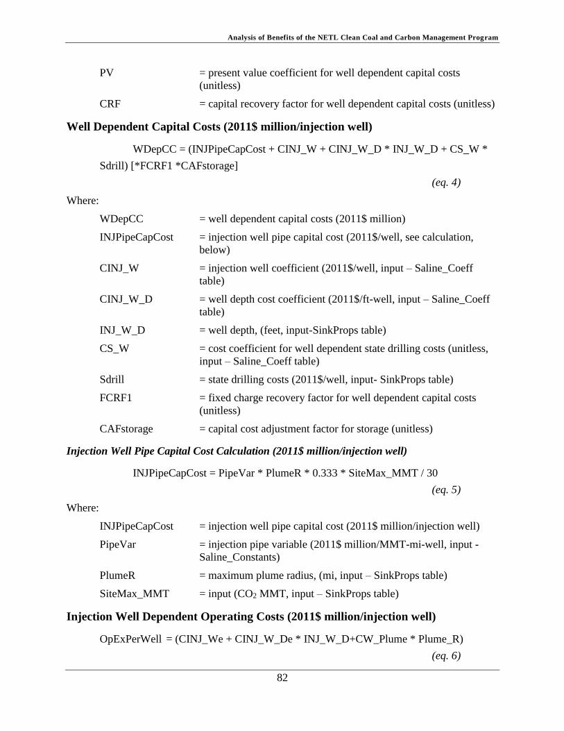
Analysis of Benefits of the NETL Clean Coal and Carbon Management Program
82
PV = present value coefficient for well dependent capital costs
(unitless)
CRF = capital recovery factor for well dependent capital costs (unitless)
Well Dependent Capital Costs (2011$ million/injection well)
WDepCC = (INJPipeCapCost + CINJ_W + CINJ_W_D * INJ_W_D + CS_W *
Sdrill) [*FCRF1 *CAFstorage]
(eq. 4)
Where:
WDepCC = well dependent capital costs (2011$ million)
INJPipeCapCost = injection well pipe capital cost (2011$/well, see calculation,
below)
CINJ_W = injection well coefficient (2011$/well, input – Saline_Coeff
table)
CINJ_W_D = well depth cost coefficient (2011$/ft-well, input – Saline_Coeff
table)
INJ_W_D = well depth, (feet, input-SinkProps table)
CS_W = cost coefficient for well dependent state drilling costs (unitless,
input – Saline_Coeff table)
Sdrill = state drilling costs (2011$/well, input- SinkProps table)
FCRF1 = fixed charge recovery factor for well dependent capital costs
(unitless)
CAFstorage = capital cost adjustment factor for storage (unitless)
Injection Well Pipe Capital Cost Calculation (2011$ million/injection well)
INJPipeCapCost = PipeVar * PlumeR * 0.333 * SiteMax_MMT / 30
(eq. 5)
Where:
INJPipeCapCost = injection well pipe capital cost (2011$ million/injection well)
PipeVar = injection pipe variable (2011$ million/MMT-mi-well, input -
Saline_Constants)
PlumeR = maximum plume radius, (mi, input – SinkProps table)
SiteMax_MMT = input (CO2 MMT, input – SinkProps table)
Injection Well Dependent Operating Costs (2011$ million/injection well)
OpExPerWell = (CINJ_We + CINJ_W_De * INJ_W_D+CW_Plume * Plume_R)
(eq. 6)

Analysis of Benefits of the NETL Clean Coal and Carbon Management Program
83
Where:
OpExPerWell = injection well dependent operating costs (2011$ million/injection
well)
CINJ_We = cost coefficient for well dependent expense (2011$ million/well,
input – Saline_Coeff table)
CINJ_W_De = cost coefficient for well and depth dependent expense (2011$
million/ft-well, input – Saline_Coeff table)
INJ_W_D = injection depth (feet, input – SinkProps table)
CW_Plume = cost coefficient for well plume (2011$ million/mi – well, input –
Saline_Coeff table)
Plume_R = plume radius (mile, input – SinkProps table)
Injection Well Dependent PISC Costs (2011$ million/well)
A detailed discussion of the treatment of PISC costs is provided in the PISC Costs section below.
WellDepFinResp = Fin_Ind / FV_annuity (eq. 7)
Where:
WellDepFinResp = injection well dependent post injection site care costs (2011$
million/well)
Fin_ind = constant fixed cost for financial responsibility (FR) (2011$
million, input – SinkProps table)
FVannuity = PISC annuitization factor @ 6.2% assuming a 30-year life of the
site, or 81.898 (see calculation, below)
PISC Annuitization Factor (“FVannuity”, unitless)
FVannuity = ((1 + FRFr)Storage – 1) / FRFr (eq. 8)
Where:
FVannuity = post injection site care annuitization factor (unitless)
FRFr = discount rate (unitless, input – FRFr table)
Storage = economic life of a saline storage site (years, input – Life table)
Variable Injection Cost Calculations (“InjectCost,” 2011$/tonne)
Variable injection costs are dependent upon the volume of CO2 injected into the saline storage
site. Each of these costs is accounted for on a per tonne basis.
InjectCost = OP3YRCC + OP5YRCC + OpExPerTon (eq. 9)
Where:
InjectCost = variable injection cost (2011$/tonne)
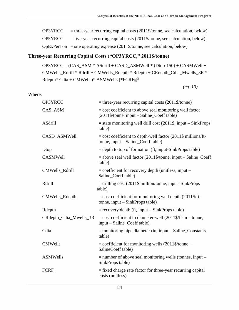
Analysis of Benefits of the NETL Clean Coal and Carbon Management Program
84
OP3YRCC = three-year recurring capital costs (2011$/tonne, see calculation, below)
OP5YRCC = five-year recurring capital costs (2011$/tonne, see calculation, below)
OpExPerTon = site operating expense (2011$/tonne, see calculation, below)
Three-year Recurring Capital Costs (“OP3YRCC,” 2011$/tonne)
OP3YRCC = (CAS_ASM * ASdrill + CASD_ASMWell * (Dtop-150) + CASMWell +
CMWells_Rdrill * Rdrill + CMWells_Rdepth * Rdepth + CRdepth_Cdia_Mwells_3R *
Rdepth* Cdia + CMWells)* ASMWells [*FCRF8]3
(eq. 10)
Where:
OP3YRCC = three-year recurring capital costs (2011$/tonne)
CAS_ASM = cost coefficient to above seal monitoring well factor
(2011$/tonne, input – Saline_Coeff table)
ASdrill = state monitoring well drill cost (2011$, input – SinkProps
table)
CASD_ASMWell = cost coefficient to depth-well factor (2011$ millions/ft-
tonne, input – Saline_Coeff table)
Dtop = depth to top of formation (ft, input-SinkProps table)
CASMWell = above seal well factor (2011$/tonne, input – Saline_Coeff
table)
CMWells_Rdrill = coefficient for recovery depth (unitless, input –
Saline_Coeff table)
Rdrill = drilling cost (2011$ million/tonne, input- SinkProps
table)
CMWells_Rdepth = cost coefficient for monitoring well depth (2011$/ft-
tonne, input – SinkProps table)
Rdepth = recovery depth (ft, input – SinkProps table)
CRdepth_Cdia_Mwells_3R = cost coefficient to diameter-well (2011$/ft-in – tonne,
input – Saline_Coeff table)
Cdia = monitoring pipe diameter (in, input – Saline_Constants
table)
CMWells = coefficient for monitoring wells (2011$/tonne –
SalineCoeff table)
ASMWells = number of above seal monitoring wells (tonnes, input –
SinkProps table)
FCRF8 = fixed charge rate factor for three-year recurring capital
costs (unitless)
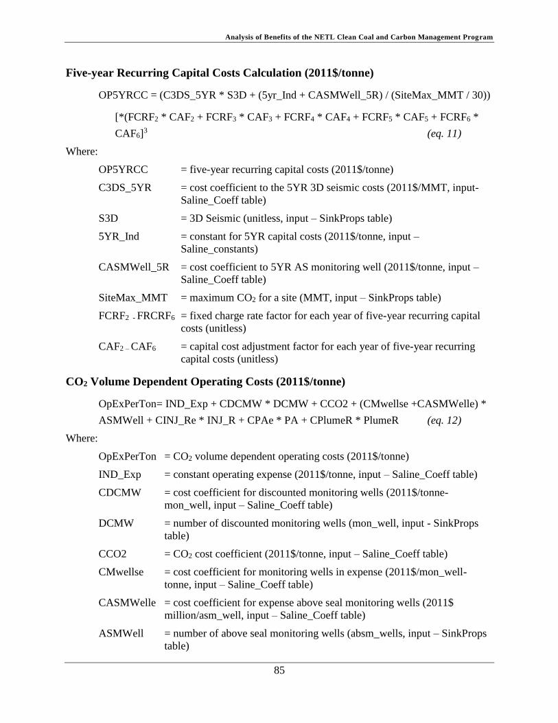
Analysis of Benefits of the NETL Clean Coal and Carbon Management Program
85
Five-year Recurring Capital Costs Calculation (2011$/tonne)
OP5YRCC = (C3DS_5YR * S3D + (5yr_Ind + CASMWell_5R) / (SiteMax_MMT / 30))
[*(FCRF2 * CAF2 + FCRF3 * CAF3 + FCRF4 * CAF4 + FCRF5 * CAF5 + FCRF6 *
CAF6]3 (eq. 11)
Where:
OP5YRCC = five-year recurring capital costs (2011$/tonne)
C3DS_5YR = cost coefficient to the 5YR 3D seismic costs (2011$/MMT, input-
Saline_Coeff table)
S3D = 3D Seismic (unitless, input – SinkProps table)
5YR_Ind = constant for 5YR capital costs (2011$/tonne, input –
Saline_constants)
CASMWell_5R = cost coefficient to 5YR AS monitoring well (2011$/tonne, input –
Saline_Coeff table)
SiteMax_MMT = maximum CO2 for a site (MMT, input – SinkProps table)
FCRF2 - FRCRF6 = fixed charge rate factor for each year of five-year recurring capital
costs (unitless)
CAF2 – CAF6 = capital cost adjustment factor for each year of five-year recurring
capital costs (unitless)
CO2 Volume Dependent Operating Costs (2011$/tonne)
OpExPerTon= IND_Exp + CDCMW * DCMW + CCO2 + (CMwellse +CASMWelle) *
ASMWell + CINJ_Re * INJ_R + CPAe * PA + CPlumeR * PlumeR (eq. 12)
Where:
OpExPerTon = CO2 volume dependent operating costs (2011$/tonne)
IND_Exp = constant operating expense (2011$/tonne, input – Saline_Coeff table)
CDCMW = cost coefficient for discounted monitoring wells (2011$/tonne-
mon_well, input – Saline_Coeff table)
DCMW = number of discounted monitoring wells (mon_well, input - SinkProps
table)
CCO2 = CO2 cost coefficient (2011$/tonne, input – Saline_Coeff table)
CMwellse = cost coefficient for monitoring wells in expense (2011$/mon_well-
tonne, input – Saline_Coeff table)
CASMWelle = cost coefficient for expense above seal monitoring wells (2011$
million/asm_well, input – Saline_Coeff table)
ASMWell = number of above seal monitoring wells (absm_wells, input – SinkProps
table)

Analysis of Benefits of the NETL Clean Coal and Carbon Management Program
86
CINJ_Re = cost coefficient for injection rate expense (2011$/MMT-tonne, input –
Saline_Coeff table)
INJ_R = injection rate (MMT/yr, input – SinkProps table)
CPAe = cost coefficient for plume area expense (2011$/mile-tonne, input –
Saline_Coeff table)
PA =plume area (mi, input – SinkProps table)
CPlumeR = cost coefficient for plume radius (2011$/mile-tonne, input –
Saline_Coeff table)
PlumeR = plume radius (mi, input – SinkProps table)
PISC Costs
Once commercial operation of the saline storage site is complete, a period of PISC begins.
During this period the site and surrounding area are monitored for 50 years in accordance with
the Environmental Protection Agency’s (EPA) regulations. Sufficient funding needs to be in
place at the start of PISC to cover all costs expected to be incurred during this period. The
variable that represents this cost (WellDepFinResp) in CTUS-NEMS is a function of the number
of injection wells drilled, which is directly proportional to the amount of CO2 stored at the site.
The per-well figure (Fin_Ind) is calculated exogenously and is an input to the model. The input
number is the discounted costkk of all costs incurred during the PISC, assuming the maximum
plume size of a site (100 mi2), divided by the number of injection wells required. The resulting
number is then annuitized and ultimately multiplied by the number of wells drilled in each year
of operation.
Fin_Ind = ∑ DiscPISCCosts(t)/wellmax50t=0 (eq. 13)
Where:
Fin_Ind = PISC well dependent input variable (2011$ millions, input-
SinkProps)
t = year in PISC period
DiscPISCCosts = PISC costs incurred in PISC period, discounted to the beginning of
the PISC period at a rate of 6.2% (2011$ millions)
wellmax = the number of injection wells required assuming the maximum
plume size (100 mi2) at the site
The Fin_Ind variable is simply placed into the WellDepFinResp variable used in the model and
then annuitized assuming a 30-year operational period of the site.
WellDepFinResp = Fin_Ind / FV_annuity (eq. 14)
Where:
kk All costs incurred during the PISC, discounted at an assumed interest rate of 6.2 percent (10-year Treasury + 200 basis point).

Analysis of Benefits of the NETL Clean Coal and Carbon Management Program
87
WellDepFinResp = well dependent financial responsibility variable (unitless)
Fin_Ind = constant fixed cost for financial responsibility (2011$ million,
input – SinkProps table)
FVannuity = annuitization factor @ 6.2% assuming a 30-year life of the site,
or 81.898 (unitless)
Well Number Calculation
The number of injection wells required is calculated in the saline formulation and is dependent
upon the amount of CO2 injection.
Wells = Maximum of 4 or CO2 * 1.5 / Maxwellinjrate (eq. 15)
Where:
Wells = number of wells
4 = minimum number of wells at an injection site
CO2 = amount of CO2 injected at site per year (MMT/yr)
Maxwellinjrate = max amount of CO2 that can be injected into a well (MMT/yr,
input - SinkProps)
Crosswalk and Validation
The crosswalk and validation of the CTUS-NEMS formation of the NETL Saline Model costs
each provide a different service in the verification of the reasonableness of the CTUS-NEMS
formulation. The crosswalk provides a direct mapping of NETL Saline Model line items to the
equations in CTUS NEMS, while the validation confirms that the results from a CTUS-NEMS
model run are comparable to those achieved through running the NETL Saline Model.
Crosswalk
A crosswalk is meant to match cost items found in the NETL Saline Model to their
representation in CTUS-NEMS. This provides a transparent map from one model to the other.
Because financial assumptions and treatment differ between NETL Saline Model and the CTUS-
NEMS saline formulation, this crosswalk is performed on costs prior to the application of any
financial treatment.
Mapping NETL Saline Model Costs to CTUS-NEMS Equations
The CTUS-NEMS saline formulation consists of several reduced-form equations that represent
the costs in the NETL Saline Model, each of which is described in the Costs subsections above.
The sections that follow map each of the NETL Saline Model costs to its associated equation in
CTUS-NEMS.
Mapping of Fixed New Injection Site Costs
Fixed new injection site costs are represented by the equation
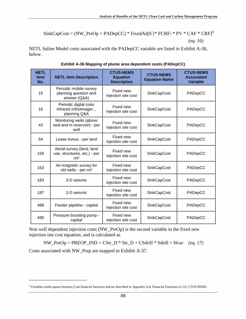
Analysis of Benefits of the NETL Clean Coal and Carbon Management Program
88
SinkCapCost = (NW_PreOp + PADepCC) * FixedAdjS [* FCRF7 * PV * CAF * CRF]ll
(eq. 16)
NETL Saline Model costs associated with the PADepCC variable are listed in Exhibit A-36,
below.
Exhibit A-36 Mapping of plume area dependent costs (PADepCC)
NETL Item No.
NETL Item Description CTUS-NEMS
Equation Description
CTUS-NEMS Equation Name
CTUS-NEMS Associated
Variable
15 Periodic mobile survey planning question and
answer (Q&A)
Fixed new injection site cost
SinkCapCost PADepCC
16 Periodic digital color
infrared orthoimager.., planning Q&A
Fixed new injection site cost
SinkCapCost PADepCC
43 Monitoring wells (above
seal and in reservoir) - per well
Fixed new injection site cost
SinkCapCost PADepCC
54 Lease bonus - per land Fixed new
injection site cost SinkCapCost PADepCC
159 Aerial survey (land, land
use, structures, etc.) - per mi2
Fixed new injection site cost
SinkCapCost PADepCC
163 Air-magnetic survey for
old wells - per mi2 Fixed new
injection site cost SinkCapCost PADepCC
183 3-D seismic Fixed new
injection site cost SinkCapCost PADepCC
187 2-D seismic Fixed new
injection site cost SinkCapCost PADepCC
488 Feeder pipeline - capital Fixed new
injection site cost SinkCapCost PADepCC
490 Pressure boosting pump -
capital Fixed new
injection site cost SinkCapCost PADepCC
Non well dependent injection costs (NW_PreOp) is the second variable in the fixed new
injection site cost equation, and is calculated as
NW_PreOp = PREOP_IND + CStr_D * Str_D + CSdrill * Sdrill + Hvar (eq. 17)
Costs associated with NW_Prep are mapped in Exhibit A-37.
ll Variables inside square brackets [] are financial functions and are described in Appendix A.8: Financial Functions in CO2 CTUS-NEMS.
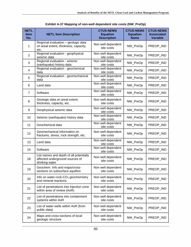
Analysis of Benefits of the NETL Clean Coal and Carbon Management Program
89
Exhibit A-37 Mapping of non-well dependent site costs (NW_PreOp)
NETL Item No.
NETL Item Description CTUS-NEMS
Equation Description
CTUS-NEMS Equation
Name
CTUS-NEMS Associated
Variable
1 Regional evaluation – geologic data on areal extent, thickness, capacity, etc.
Non well dependent site costs
NW_PreOp PREOP_IND
2 Regional evaluation - geophysical seismic data
Non well dependent site costs
NW_PreOp PREOP_IND
3 Regional evaluation - seismic (earthquake) history data
Non well dependent site costs
NW_PreOp PREOP_IND
4 Regional evaluation - geochemical data
Non well dependent site costs
NW_PreOp PREOP_IND
5 Regional evaluation - geomechanical data
Non well dependent site costs
NW_PreOp PREOP_IND
6 Land data Non well dependent
site costs NW_PreOp PREOP_IND
7 Software Non well dependent
site costs NW_PreOp PREOP_IND
8 Geologic data on areal extent, thickness, capacity, etc.
Non well dependent site costs
NW_PreOp PREOP_IND
9 Geophysical seismic data Non well dependent
site costs NW_PreOp PREOP_IND
10 Seismic (earthquake) history data Non well dependent
site costs NW_PreOp PREOP_IND
11 Geochemical data Non well dependent
site costs NW_PreOp PREOP_IND
12 Geomechanical information on fractures, stress, rock strength, etc.
Non well dependent site costs
NW_PreOp PREOP_IND
13 Land data Non well dependent
site costs NW_PreOp PREOP_IND
14 Software Non well dependent
site costs NW_PreOp PREOP_IND
18 List names and depth of all potentially affected underground sources of drinking water
Non well dependent site costs
NW_PreOp PREOP_IND
19 Geochem. Info and maps/cross-sections on subsurface aquifers
Non well dependent site costs
NW_PreOp PREOP_IND
20 Info on water-rock-CO2 geochemistry and mineral reactions
Non well dependent site costs
NW_PreOp PREOP_IND
21 List of penetrations into injection zone within area of review (AoR)
Non well dependent site costs
NW_PreOp PREOP_IND
22 List of penetrations into containment systems within AoR
Non well dependent site costs
NW_PreOp PREOP_IND
23 List of water wells within AoR (from public data)
Non well dependent site costs
NW_PreOp PREOP_IND
24 Maps and cross-sections of local geologic structure
Non well dependent site costs
NW_PreOp PREOP_IND
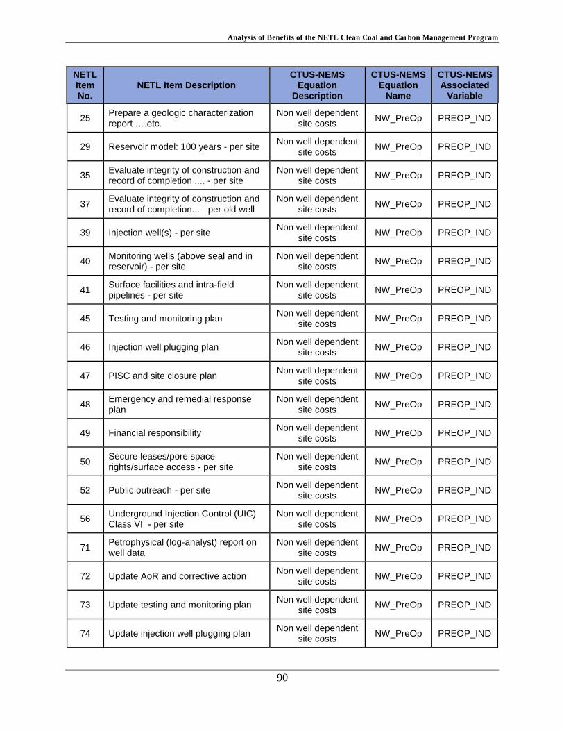
Analysis of Benefits of the NETL Clean Coal and Carbon Management Program
90
NETL Item No.
NETL Item Description CTUS-NEMS
Equation Description
CTUS-NEMS Equation
Name
CTUS-NEMS Associated
Variable
25 Prepare a geologic characterization report ….etc.
Non well dependent site costs
NW_PreOp PREOP_IND
29 Reservoir model: 100 years - per site Non well dependent
site costs NW_PreOp PREOP_IND
35 Evaluate integrity of construction and record of completion .... - per site
Non well dependent site costs
NW_PreOp PREOP_IND
37 Evaluate integrity of construction and record of completion... - per old well
Non well dependent site costs
NW_PreOp PREOP_IND
39 Injection well(s) - per site Non well dependent
site costs NW_PreOp PREOP_IND
40 Monitoring wells (above seal and in reservoir) - per site
Non well dependent site costs
NW_PreOp PREOP_IND
41 Surface facilities and intra-field pipelines - per site
Non well dependent site costs
NW_PreOp PREOP_IND
45 Testing and monitoring plan Non well dependent
site costs NW_PreOp PREOP_IND
46 Injection well plugging plan Non well dependent
site costs NW_PreOp PREOP_IND
47 PISC and site closure plan Non well dependent
site costs NW_PreOp PREOP_IND
48 Emergency and remedial response plan
Non well dependent site costs
NW_PreOp PREOP_IND
49 Financial responsibility Non well dependent
site costs NW_PreOp PREOP_IND
50 Secure leases/pore space rights/surface access - per site
Non well dependent site costs
NW_PreOp PREOP_IND
52 Public outreach - per site Non well dependent
site costs NW_PreOp PREOP_IND
56 Underground Injection Control (UIC) Class VI - per site
Non well dependent site costs
NW_PreOp PREOP_IND
71 Petrophysical (log-analyst) report on well data
Non well dependent site costs
NW_PreOp PREOP_IND
72 Update AoR and corrective action Non well dependent
site costs NW_PreOp PREOP_IND
73 Update testing and monitoring plan Non well dependent
site costs NW_PreOp PREOP_IND
74 Update injection well plugging plan Non well dependent
site costs NW_PreOp PREOP_IND
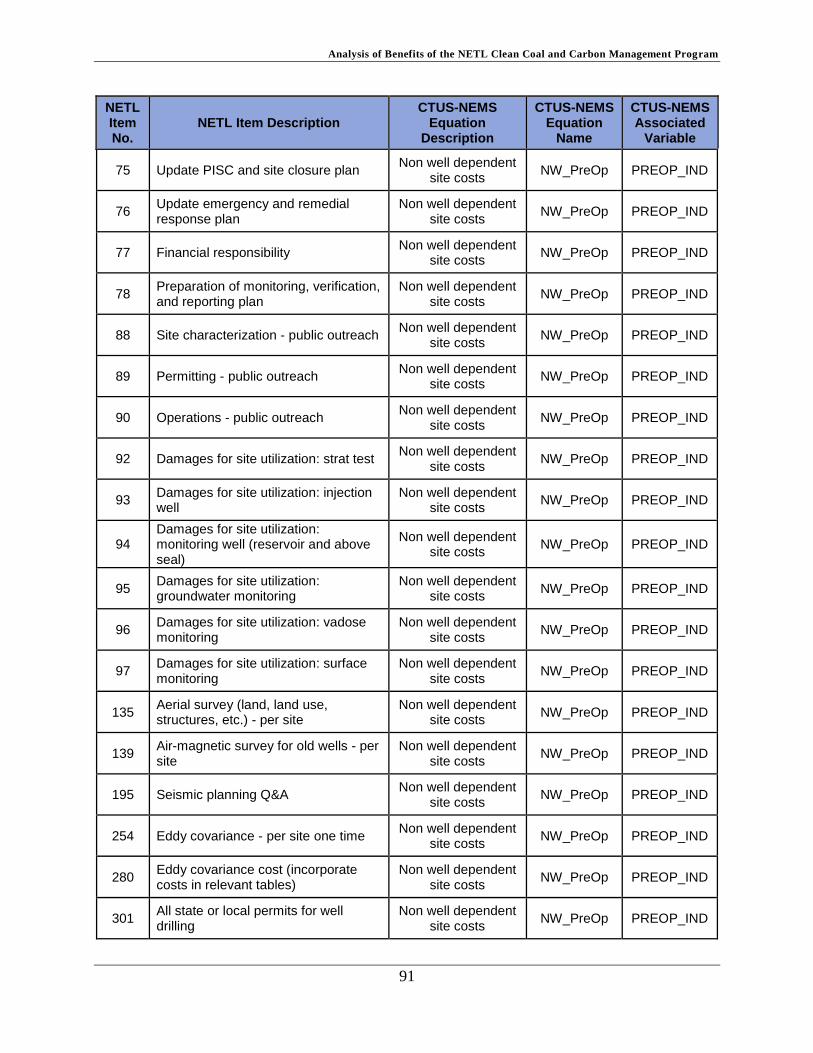
Analysis of Benefits of the NETL Clean Coal and Carbon Management Program
91
NETL Item No.
NETL Item Description CTUS-NEMS
Equation Description
CTUS-NEMS Equation
Name
CTUS-NEMS Associated
Variable
75 Update PISC and site closure plan Non well dependent
site costs NW_PreOp PREOP_IND
76 Update emergency and remedial response plan
Non well dependent site costs
NW_PreOp PREOP_IND
77 Financial responsibility Non well dependent
site costs NW_PreOp PREOP_IND
78 Preparation of monitoring, verification, and reporting plan
Non well dependent site costs
NW_PreOp PREOP_IND
88 Site characterization - public outreach Non well dependent
site costs NW_PreOp PREOP_IND
89 Permitting - public outreach Non well dependent
site costs NW_PreOp PREOP_IND
90 Operations - public outreach Non well dependent
site costs NW_PreOp PREOP_IND
92 Damages for site utilization: strat test Non well dependent
site costs NW_PreOp PREOP_IND
93 Damages for site utilization: injection well
Non well dependent site costs
NW_PreOp PREOP_IND
94 Damages for site utilization: monitoring well (reservoir and above seal)
Non well dependent site costs
NW_PreOp PREOP_IND
95 Damages for site utilization: groundwater monitoring
Non well dependent site costs
NW_PreOp PREOP_IND
96 Damages for site utilization: vadose monitoring
Non well dependent site costs
NW_PreOp PREOP_IND
97 Damages for site utilization: surface monitoring
Non well dependent site costs
NW_PreOp PREOP_IND
135 Aerial survey (land, land use, structures, etc.) - per site
Non well dependent site costs
NW_PreOp PREOP_IND
139 Air-magnetic survey for old wells - per site
Non well dependent site costs
NW_PreOp PREOP_IND
195 Seismic planning Q&A Non well dependent
site costs NW_PreOp PREOP_IND
254 Eddy covariance - per site one time Non well dependent
site costs NW_PreOp PREOP_IND
280 Eddy covariance cost (incorporate costs in relevant tables)
Non well dependent site costs
NW_PreOp PREOP_IND
301 All state or local permits for well drilling
Non well dependent site costs
NW_PreOp PREOP_IND

Analysis of Benefits of the NETL Clean Coal and Carbon Management Program
92
NETL Item No.
NETL Item Description CTUS-NEMS
Equation Description
CTUS-NEMS Equation
Name
CTUS-NEMS Associated
Variable
314 Cost to drill and complete from American Petroleum Institute (API)
Non well dependent site costs
NW_PreOp Csdrill
340 Total cost of all wireline logging Non well dependent
site costs NW_PreOp CStr_D
353 Total cost of all coring activities Non well dependent
site costs NW_PreOp PREOP_IND
366 Cost of fluid samples Non well dependent
site costs NW_PreOp PREOP_IND
379 Total cost of all well tests Non well dependent
site costs NW_PreOp PREOP_IND
392 Vertical seismic profile (VSP) for characterization
Non well dependent site costs
NW_PreOp PREOP_IND
479 Total costs for plugging & abandoning wells
Non well dependent site costs
NW_PreOp PREOP_IND
492 Header - capital Non well dependent
site costs NW_PreOp Hvar
496 Office building - capital Non well dependent
site costs NW_PreOp PREOP_IND
498 Control systems – capital Non well dependent
site costs NW_PreOp PREOP_IND
500 Access road to building - capital Non well dependent
site costs NW_PreOp PREOP_IND
Mapping of Well Dependent Costs
Well dependent costs are discussed in the Well Dependent Cost Calculation section above and
are represented in CTUS-NEMS as
WellCapCost = (WDepCC + OpExPerWell + WellDepFinResp) * FixedAdjS [* PV * CRF]
(eq. 18)
The mapping of each of the major cost variables in WellCapCost equation will be addressed
separately.
The first variable in the well dependent cost equation is well dependent capital costs (in 2011$
million/injection well) which are calculated as
WDepCC = (INJPipeCapCost + CINJ_W + CINJ_W_D * INJ_W_D + CS_W * Sdrill)
[*FCRF1 *CAFstorage] (eq. 19)
and are mapped in Exhibit A-38.
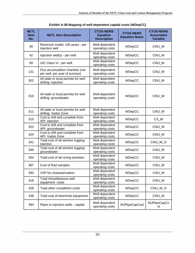
Analysis of Benefits of the NETL Clean Coal and Carbon Management Program
93
Exhibit A-38 Mapping of well dependent capital costs (WDepCC)
NETL Item No.
NETL Item Description CTUS-NEMS
Equation Description
CTUS-NEMS Equation Name
CTUS-NEMS Associated
Variable
30 Reservoir model: 100 years - per injection well
Well dependent operating costs
WDepCC CINJ_W
42 Injection well(s) - per well Well dependent operating costs
WDepCC CINJ_W
69 UIC Class VI - per well Well dependent operating costs
WDepCC CINJ_W
131 Flux accumulation chamber (not per well, per year of surveys)
Well dependent operating costs
WDepCC CINJ_W
302 All state or local permits for well drilling: Injection
Well dependent operating costs
WDepCC CINJ_W
310 All state or local permits for well drilling: groundwater
Well dependent operating costs
WDepCC CINJ_W
311 All state or local permits for well drilling: Vados Zone
Well dependent operating costs
WDepCC CINJ_W
315 Cost to drill and complete from API: injection
Well dependent operating costs
WDepCC CS_W
323 Cost to drill and complete from API: groundwater
Well dependent operating costs
WDepCC CINJ_W
324 Cost to drill and complete from API: Vados Zone
Well dependent operating costs
WDepCC CINJ_W
341 Total cost of all wireline logging: injection
Well dependent operating costs
WDepCC CINJ_W_D
349 Total cost of all wireline logging: groundwater
Well dependent operating costs
WDepCC CINJ_W
354 Total cost of all coring activities Well dependent operating costs
WDepCC CINJ_W
367 Cost of fluid samples Well dependent operating costs
WDepCC CINJ_W
393 VSP for characterization Well dependent operating costs
WDepCC CINJ_W
416 Total miscellaneous well equipment costs
Well dependent operating costs
WDepCC CINJ_W
428 Total other completion costs Well dependent operating costs
WDepCC CINJ_W_D
438 Total cost of downhole equipment Well dependent operating costs
WDepCC CINJ_W
494 Pipes to injection wells - capital Well dependent operating costs
INJPipeCapCost INJPipeCapCo
st
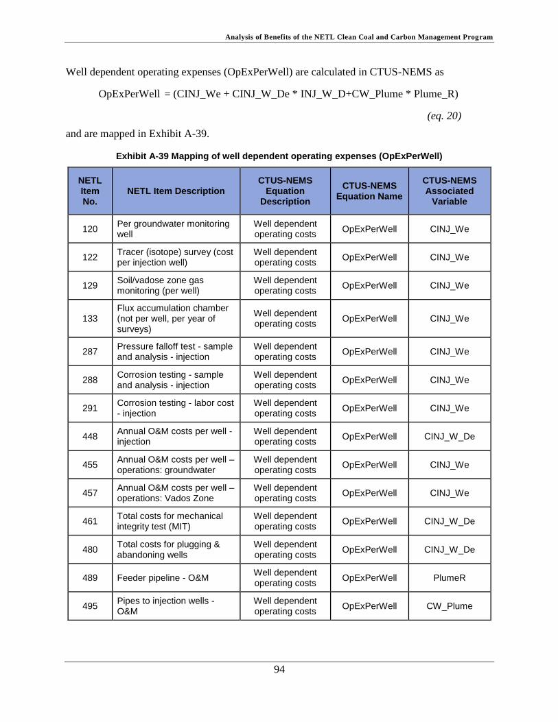
Analysis of Benefits of the NETL Clean Coal and Carbon Management Program
94
Well dependent operating expenses (OpExPerWell) are calculated in CTUS-NEMS as
OpExPerWell = (CINJ_We + CINJ_W_De * INJ_W_D+CW_Plume * Plume_R)
(eq. 20)
and are mapped in Exhibit A-39.
Exhibit A-39 Mapping of well dependent operating expenses (OpExPerWell)
NETL Item No.
NETL Item Description CTUS-NEMS
Equation Description
CTUS-NEMS Equation Name
CTUS-NEMS Associated
Variable
120 Per groundwater monitoring well
Well dependent operating costs
OpExPerWell CINJ_We
122 Tracer (isotope) survey (cost per injection well)
Well dependent operating costs
OpExPerWell CINJ_We
129 Soil/vadose zone gas monitoring (per well)
Well dependent operating costs
OpExPerWell CINJ_We
133 Flux accumulation chamber (not per well, per year of surveys)
Well dependent operating costs
OpExPerWell CINJ_We
287 Pressure falloff test - sample and analysis - injection
Well dependent operating costs
OpExPerWell CINJ_We
288 Corrosion testing - sample and analysis - injection
Well dependent operating costs
OpExPerWell CINJ_We
291 Corrosion testing - labor cost - injection
Well dependent operating costs
OpExPerWell CINJ_We
448 Annual O&M costs per well - injection
Well dependent operating costs
OpExPerWell CINJ_W_De
455 Annual O&M costs per well – operations: groundwater
Well dependent operating costs
OpExPerWell CINJ_We
457 Annual O&M costs per well – operations: Vados Zone
Well dependent operating costs
OpExPerWell CINJ_We
461 Total costs for mechanical integrity test (MIT)
Well dependent operating costs
OpExPerWell CINJ_W_De
480 Total costs for plugging & abandoning wells
Well dependent operating costs
OpExPerWell CINJ_W_De
489 Feeder pipeline - O&M Well dependent operating costs
OpExPerWell PlumeR
495 Pipes to injection wells - O&M
Well dependent operating costs
OpExPerWell CW_Plume

Analysis of Benefits of the NETL Clean Coal and Carbon Management Program
95
The injection well dependent PISC costs (WellDepFinResp) are calculated as
WellDepFinResp = Fin_Ind/FV_annuity (eq. 21)
and are mapped in Exhibit A-40.
Exhibit A-40 Mapping of well dependent PISC costs (WellDepFinResp)
NETL Item No.
NETL Item Description CTUS-NEMS
Equation Description
CTUS-NEMS Equation Name
CTUS-NEMS Associated
Variable
80 Subpart RR - PISC PISC Costs WellDepFinResp Fin_Ind
91 Public outreach PISC Costs WellDepFinResp Fin_Ind
101 Subpart RR PISC Costs WellDepFinResp Fin_Ind
111 Post -injection monitoring PISC Costs WellDepFinResp Fin_Ind
113 Site closure report PISC Costs WellDepFinResp Fin_Ind
117 Per monitoring well: dual completion PISC Costs WellDepFinResp Fin_Ind
119 Per monitoring well above seal PISC Costs WellDepFinResp Fin_Ind
121 Per groundwater monitoring well PISC Costs WellDepFinResp Fin_Ind
126 Collect pressure data from deep monitoring wells – PISC – dual completion
PISC Costs WellDepFinResp Fin_Ind
128 Collect pressure data from deep monitoring wells – PISC – above seal
PISC Costs WellDepFinResp Fin_Ind
130 Soil/vadose zone gas monitoring (per well)
PISC Costs WellDepFinResp Fin_Ind
134 Flux accumulation chamber (not per well, per year of surveys)
PISC Costs WellDepFinResp Fin_Ind
186 3-D seismic PISC Costs WellDepFinResp Fin_Ind
251 Eddy covariance - per site PISC Costs WellDepFinResp Fin_Ind
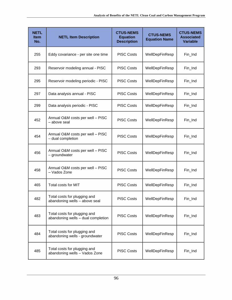
Analysis of Benefits of the NETL Clean Coal and Carbon Management Program
96
NETL Item No.
NETL Item Description CTUS-NEMS
Equation Description
CTUS-NEMS Equation Name
CTUS-NEMS Associated
Variable
255 Eddy covariance - per site one time PISC Costs WellDepFinResp Fin_Ind
293 Reservoir modeling annual - PISC PISC Costs WellDepFinResp Fin_Ind
295 Reservoir modeling periodic - PISC PISC Costs WellDepFinResp Fin_Ind
297 Data analysis annual - PISC PISC Costs WellDepFinResp Fin_Ind
299 Data analysis periodic - PISC PISC Costs WellDepFinResp Fin_Ind
452 Annual O&M costs per well – PISC – above seal
PISC Costs WellDepFinResp Fin_Ind
454 Annual O&M costs per well – PISC – dual completion
PISC Costs WellDepFinResp Fin_Ind
456 Annual O&M costs per well – PISC – groundwater
PISC Costs WellDepFinResp Fin_Ind
458 Annual O&M costs per well – PISC – Vados Zone
PISC Costs WellDepFinResp Fin_Ind
465 Total costs for MIT PISC Costs WellDepFinResp Fin_Ind
482 Total costs for plugging and abandoning wells – above seal
PISC Costs WellDepFinResp Fin_Ind
483 Total costs for plugging and abandoning wells – dual completion
PISC Costs WellDepFinResp Fin_Ind
484 Total costs for plugging and abandoning wells - groundwater
PISC Costs WellDepFinResp Fin_Ind
485 Total costs for plugging and abandoning wells – Vados Zone
PISC Costs WellDepFinResp Fin_Ind
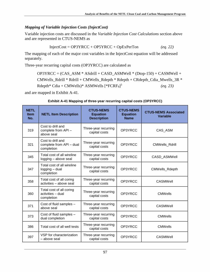
Analysis of Benefits of the NETL Clean Coal and Carbon Management Program
97
Mapping of Variable Injection Costs (InjectCost)
Variable injection costs are discussed in the Variable Injection Cost Calculations section above
and are represented in CTUS-NEMS as
InjectCost = OP3YRCC + OP5YRCC + OpExPerTon (eq. 22)
The mapping of each of the major cost variables in the InjectCost equation will be addressed
separately.
Three-year recurring capital costs (OP3YRCC) are calculated as
OP3YRCC = (CAS_ASM * ASdrill + CASD_ASMWell * (Dtop-150) + CASMWell +
CMWells_Rdrill * Rdrill + CMWells_Rdepth * Rdepth + CRdepth_Cdia_Mwells_3R *
Rdepth* Cdia + CMWells)* ASMWells [*FCRF8]3 (eq. 23)
and are mapped in Exhibit A-41.
Exhibit A-41 Mapping of three-year recurring capital costs (OP3YRCC)
NETL Item No.
NETL Item Description CTUS-NEMS
Equation Description
CTUS-NEMS Equation
Name
CTUS-NEMS Associated Variable
319 Cost to drill and complete from API – above seal
Three-year recurring capital costs
OP3YRCC CAS_ASM
321 Cost to drill and complete from API – dual completion
Three-year recurring capital costs
OP3YRCC CMWells_Rdrill
345 Total cost of all wireline logging – above seal
Three-year recurring capital costs
OP3YRCC CASD_ASMWell
347 Total cost of all wireline logging – dual completion
Three-year recurring capital costs
OP3YRCC CMWells_Rdepth
358 Total cost of all coring activities – above seal
Three-year recurring capital costs
OP3YRCC CASMWell
360 Total cost of all coring activities – dual completion
Three-year recurring capital costs
OP3YRCC CMWells
371 Cost of fluid samples – above seal
Three-year recurring capital costs
OP3YRCC CASMWell
373 Cost of fluid samples – dual completion
Three-year recurring capital costs
OP3YRCC CMWells
386 Total cost of all well tests Three-year recurring
capital costs OP3YRCC CMWells
397 VSP for characterization – above seal
Three-year recurring capital costs
OP3YRCC CASMWell

Analysis of Benefits of the NETL Clean Coal and Carbon Management Program
98
NETL Item No.
NETL Item Description CTUS-NEMS
Equation Description
CTUS-NEMS Equation
Name
CTUS-NEMS Associated Variable
399 VSP for characterization – dual completion
Three-year recurring capital costs
OP3YRCC CMWells
434 Total other completion costs
Three-year recurring capital costs
OP3YRCC CRdepth_Cdia_Mwells_3R
442 Total cost of downhole equipment – above seal
Three-year recurring capital costs
OP3YRCC CASMWell
444 Total cost of downhole equipment – dual completion
Three-year recurring capital costs
OP3YRCC CMWells
Five-year recurring capital costs (OP5YRCC) are calculated as
OP5YRCC = (C3DS_5YR * S3D + (5yr_Ind + CASMWell_5R) / (SiteMax_MMT / 30))
[*(FCRF2 * CAF2 + FCRF3 * CAF3 + FCRF4 * CAF4 + FCRF5 * CAF5 + FCRF6 *
CAF6]3 (eq. 24)
and are mapped in Exhibit A-42.
Exhibit A-42 Mapping of five-year recurring capital costs (OP5YRCC)
NETL Item No.
NETL Item Description CTUS-NEMS
Equation Description
CTUS-NEMS Equation Name
CTUS-NEMS Associated
Variable
79 Subpart RR - operations Five-year recurring
capital costs OP5YRCC 5yr_Ind
102 AoR and corrective action plan
Five-year recurring capital costs
OP5YRCC 5yr_Ind
104 Testing and monitoring plan
Five-year recurring capital costs
OP5YRCC 5yr_Ind
106 Emergency and remedial response plan
Five-year recurring capital costs
OP5YRCC 5yr_Ind
185 3-D seismic Five-year recurring
capital costs OP5YRCC C3DS_5YR * S3D
306 All state or local permits for well drilling
Five-year recurring capital costs
OP5YRCC CASMWell_5R
308 All state or local permits for well drilling
Five-year recurring capital costs
OP5YRCC CASMWell_5R
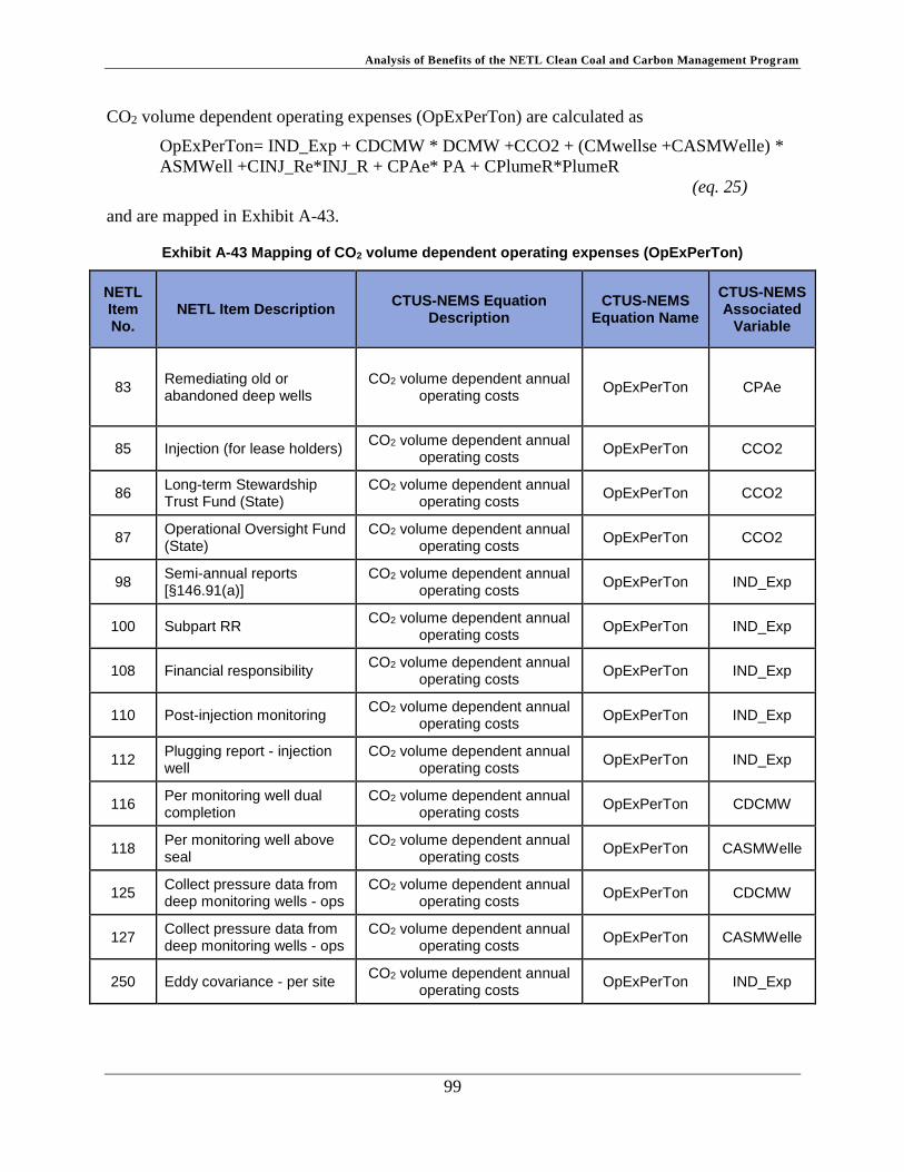
Analysis of Benefits of the NETL Clean Coal and Carbon Management Program
99
CO2 volume dependent operating expenses (OpExPerTon) are calculated as
OpExPerTon= IND_Exp + CDCMW * DCMW +CCO2 + (CMwellse +CASMWelle) *
ASMWell +CINJ_Re*INJ_R + CPAe* PA + CPlumeR*PlumeR
(eq. 25)
and are mapped in Exhibit A-43.
Exhibit A-43 Mapping of CO2 volume dependent operating expenses (OpExPerTon)
NETL Item No.
NETL Item Description CTUS-NEMS Equation
Description CTUS-NEMS
Equation Name
CTUS-NEMS Associated
Variable
83 Remediating old or abandoned deep wells
CO2 volume dependent annual operating costs
OpExPerTon CPAe
85 Injection (for lease holders) CO2 volume dependent annual
operating costs OpExPerTon CCO2
86 Long-term Stewardship Trust Fund (State)
CO2 volume dependent annual operating costs
OpExPerTon CCO2
87 Operational Oversight Fund (State)
CO2 volume dependent annual operating costs
OpExPerTon CCO2
98 Semi-annual reports [§146.91(a)]
CO2 volume dependent annual operating costs
OpExPerTon IND_Exp
100 Subpart RR CO2 volume dependent annual
operating costs OpExPerTon IND_Exp
108 Financial responsibility CO2 volume dependent annual
operating costs OpExPerTon IND_Exp
110 Post-injection monitoring CO2 volume dependent annual
operating costs OpExPerTon IND_Exp
112 Plugging report - injection well
CO2 volume dependent annual operating costs
OpExPerTon IND_Exp
116 Per monitoring well dual completion
CO2 volume dependent annual operating costs
OpExPerTon CDCMW
118 Per monitoring well above seal
CO2 volume dependent annual operating costs
OpExPerTon CASMWelle
125 Collect pressure data from deep monitoring wells - ops
CO2 volume dependent annual operating costs
OpExPerTon CDCMW
127 Collect pressure data from deep monitoring wells - ops
CO2 volume dependent annual operating costs
OpExPerTon CASMWelle
250 Eddy covariance - per site CO2 volume dependent annual
operating costs OpExPerTon IND_Exp
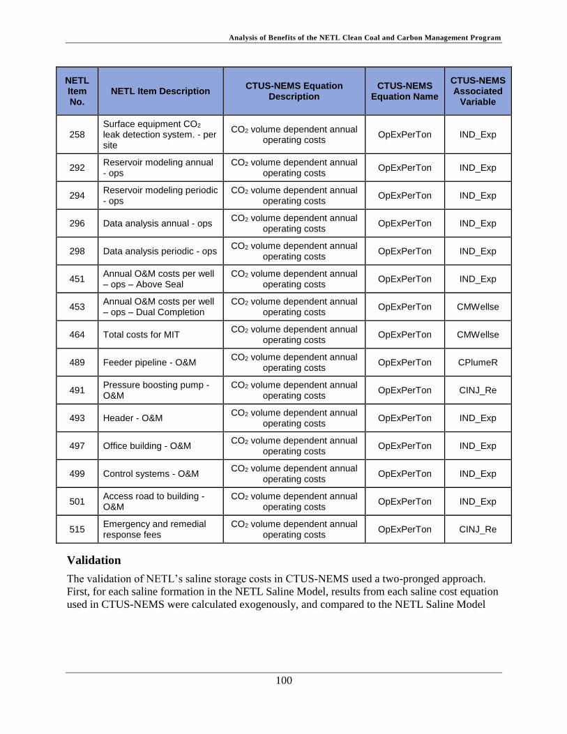
Analysis of Benefits of the NETL Clean Coal and Carbon Management Program
100
NETL Item No.
NETL Item Description CTUS-NEMS Equation
Description CTUS-NEMS
Equation Name
CTUS-NEMS Associated
Variable
258 Surface equipment CO2 leak detection system. - per site
CO2 volume dependent annual operating costs
OpExPerTon IND_Exp
292 Reservoir modeling annual - ops
CO2 volume dependent annual operating costs
OpExPerTon IND_Exp
294 Reservoir modeling periodic - ops
CO2 volume dependent annual operating costs
OpExPerTon IND_Exp
296 Data analysis annual - ops CO2 volume dependent annual
operating costs OpExPerTon IND_Exp
298 Data analysis periodic - ops CO2 volume dependent annual
operating costs OpExPerTon IND_Exp
451 Annual O&M costs per well – ops – Above Seal
CO2 volume dependent annual operating costs
OpExPerTon IND_Exp
453 Annual O&M costs per well – ops – Dual Completion
CO2 volume dependent annual operating costs
OpExPerTon CMWellse
464 Total costs for MIT CO2 volume dependent annual
operating costs OpExPerTon CMWellse
489 Feeder pipeline - O&M CO2 volume dependent annual
operating costs OpExPerTon CPlumeR
491 Pressure boosting pump - O&M
CO2 volume dependent annual operating costs
OpExPerTon CINJ_Re
493 Header - O&M CO2 volume dependent annual
operating costs OpExPerTon IND_Exp
497 Office building - O&M CO2 volume dependent annual
operating costs OpExPerTon IND_Exp
499 Control systems - O&M CO2 volume dependent annual
operating costs OpExPerTon IND_Exp
501 Access road to building - O&M
CO2 volume dependent annual operating costs
OpExPerTon IND_Exp
515 Emergency and remedial response fees
CO2 volume dependent annual operating costs
OpExPerTon CINJ_Re
Validation
The validation of NETL’s saline storage costs in CTUS-NEMS used a two-pronged approach.
First, for each saline formation in the NETL Saline Model, results from each saline cost equation
used in CTUS-NEMS were calculated exogenously, and compared to the NETL Saline Model
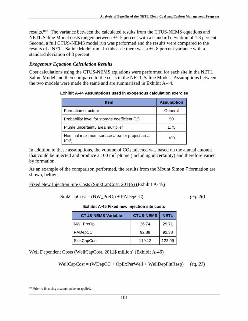
Analysis of Benefits of the NETL Clean Coal and Carbon Management Program
101
results.mm The variance between the calculated results from the CTUS-NEMS equations and
NETL Saline Model costs ranged between +/- 5 percent with a standard deviation of 1.3 percent.
Second, a full CTUS-NEMS model run was performed and the results were compared to the
results of a NETL Saline Model run. In this case there was a +/- 8 percent variance with a
standard deviation of 3 percent.
Exogenous Equation Calculation Results
Cost calculations using the CTUS-NEMS equations were performed for each site in the NETL
Saline Model and then compared to the costs in the NETL Saline Model. Assumptions between
the two models were made the same and are summarized in Exhibit A-44.
Exhibit A-44 Assumptions used in exogenous calculation exercise
Item Assumption
Formation structure General
Probability level for storage coefficient (%) 50
Plume uncertainty area multiplier 1.75
Nominal maximum surface area for project area (mi2)
100
In addition to these assumptions, the volume of CO2 injected was based on the annual amount
that could be injected and produce a 100 mi2 plume (including uncertainty) and therefore varied
by formation.
As an example of the comparison performed, the results from the Mount Simon 7 formation are
shown, below.
Fixed New Injection Site Costs (SinkCapCost, 2011$) (Exhibit A-45)
SinkCapCost = (NW_PreOp + PADepCC) (eq. 26)
Exhibit A-45 Fixed new injection site costs
CTUS-NEMS Variable CTUS-NEMS NETL
NW_PreOp 26.74 29.71
PADepCC 92.38 92.38
SinkCapCost 119.12 122.09
Well Dependent Costs (WellCapCost, 2011$ million) (Exhibit A-46)
WellCapCost = (WDepCC + OpExPerWell + WellDepFinResp) (eq. 27)
mm Prior to financing assumption being applied.

Analysis of Benefits of the NETL Clean Coal and Carbon Management Program
102
Exhibit A-46 Well dependent costs
CTUS-NEMS Variable CTUS-NEMS NETL
WDepCC 34.40 35.60
OpExPerWell 1.04 1.36
WellDepFinResp 166.19 164.17
WellCapCost 201.63 201.13
Variable Injection Costs (InjectCost, 2011$ million) (Exhibit A-47)
InjectCost = OP3YRCC + OP5YRCC + OpExPerTon (eq. 28)
Exhibit A-47 Variable injection costs
CTUS-NEMS Variable CTUS-NEMS NETL
OP3YRCC 10.61 10.39
OP5YRCC 27.38 26.70
OpExPerTon 13.07 12.19
InjectCost 51.06 49.28
Total Cost Comparison (Exhibit A-48)
Exhibit A-48 Total cost comparison
Cost CTUS-NEMS NETL
2011$/million 371.81 372.50
2011$/tonne* 7.66 7.58
*Based on 6.63 MMT annually.
Model Run Validation
To further validate the new saline storage formulation used in CTUS-NEMS, the unit cost results
of the NETL Saline Model were compared to those from the CTUS-NEMS run. For each
formation that was activated in the test run, NETL’s Saline Model was run using similar
assumptions for injection rates and volumes. The results are summarized in Exhibit A-49, below
and range between +/- 8 percent variance.

Analysis of Benefits of the NETL Clean Coal and Carbon Management Program
103
Exhibit A-49 Variance in saline storage unit costs between NETL Saline Model and CTUS-NEMS
Formation
Average Annual CO2
Injected (MMT/yr)
Unit Cost
NETL Saline Model (2011$/tonne)
CTUS-NEMS (2011$/tonne)
Variance (%)
Lower Tuscaloosa 8 2.52 9.94 10.59 -6.54%
Lower Tuscaloosa 10 22.5 7.36 7.95 -8.02%
Mount Simon 7 1.55 11.53 10.63 7.81%
Arbuckle 1 2.20 12.36 12.18 1.47%
Two major factors contribute to the variance between the models. The first involves the
behavior of the CO2 injection stream in each of the models. The NETL Saline Model assumes a
consistent flow of CO2 through the life of a project. The CO2 injection stream in CTUS-NEMS
varies over the life of a project depending upon demand for CO2 by EOR and other factors.
Because the unit cost of CO2 is evaluated over the lifetime, even if the average annual injection
rate is the same between the two models, fluctuations in the injection rate will produce a
different answer than a steady annual injection rate.
The application of financial functions and their underlying assumptions is the second factor that
affects the unit CO2 cost. Discount rates differ between the models with the NETL Saline Model
assuming a 4.98 percent discount rate while CTUS-NEMS assumes 6.2 percent. A thorough
description of the financial functions and their application in CTUS-NEMS are described in
Appendix A.8: Financial Functions in CO2 CTUS-NEMS. In addition, a specific discussion of
the financial treatment of PISC in CTUS-NEMS can be found in Appendix A.9: Estimating the
Costs Associated with Financial Responsibility Post-commercial Operation.

Analysis of Benefits of the NETL Clean Coal and Carbon Management Program
104
Appendix A.8: Financial Functions in CO2 CTUS-NEMS
Calculation of Financial Functions
Fixed Charge Rate Factor
The goal is to calculate the total net present value (NPV) life-cycle costs of a project. This NPV
cost is then converted to an annual equivalent amount that if collected would yield the same
NPV; this is typically described as its annualized cost.nn The ratio of the annualized amount to
the NPV life-cycle costs represents the fixed charge rate factor (FCRF), i.e., the proportion of the
capital related life-cycle cost that must be collected to ensure that all these costs are recovered
but no more than that. The following formulation employs some simplifying assumptions that
allow the calculation of the FCRF to be made using a series of closed form equations.
The FCRF can be estimated using the following formula:
FCRF = CRF * NPV_INV (eq. 1)
Where:
CRF = capital recovery factor (unitless)
NPV_INV = net present value of all investment-related expenses (unitless) (further
defined below)
Calculation of Capital Recovery Factor
For the purposes of carbon capture, transport, utilization, and storage (CTUS), the capital
recovery factor (CRF) is the fraction which creates an annuity over the economic life of an
investment at the equity discount rate.oo
CRF = 1 / [(1- (1 / (1 + Re) Nc)) / Re] (eq. 2)
Where:
Re = equity discount rate (unitless)
Nc = economic life of investment (yr)
nn These annualized costs can be placed on a levelized-cost basis by dividing the annualized cost by the expected annual quantity (tonnes of CO2)
handled. A slightly more complicated framework is needed if the annual quantity is not assumed to be constant over the life of the project. oo A CRF is the ratio of a constant annuity to the present value (PV) of receiving that annuity for a given length of time. The equity rate of return
is used in this formulation to allow for the debt life to be different from (presumably shorter) the economic life in the analysis. In these
circumstances, using the after-tax cost of capital would distort the calculation and bias due to the fact that debt and equity are not being evenly deployed over the economic life of the asset.

Analysis of Benefits of the NETL Clean Coal and Carbon Management Program
105
Equity Discount Rate
The equity discount rate (Re) represents the minimum required rate of return on an equity
investment. As noted earlier, alternative formulations to estimate this value are possible. A
simple approach was applied.
Re = (Rf + Pe) / 100 (eq. 3)
Where:
Rf = risk free rate (unitless)
Pe = equity rate risk premiumpp (unitless)
NPV of All Investment Related Expenses
Each of the investment-related expenses needs to be addressed including: equity returns and
associated income taxes thereon, interest expense and the associated tax deduction associated
therewith, tax depreciation and the impact on income taxes associated therewith, and debt
principal payments and associated tax implications.
This NPV (NPV_INV) captures all the capital related expenses into a single NPV value to allow
the equivalent annual amount to be calculated.
NPV_INV = E / (1-T) + IEF -(T / (1-T)) * DDEPf + DDPP / (1-T) (eq. 4)
Where:
E = equity fraction, or E* (unitless) (NPV of cash out flows from equity)
T = tax rate (unitless)
IEF = interest expense factor (unitless)
DDEPf = discounted depreciation factor (unitless)
DDPP = discounted debt principal (unitless)
Cash Out Flow from Equity
The cash out flow from equity (E) accounts for the return to equity investors. This factor is the
NPV of the cash flow from equity investors, discounted at the equity rate.
E* = Cash out flow (i) / (1+Re)i; over i = 1 to Nc (eq. 5)
Assuming only an initial equity investment at the project start, E* = E.qq
pp The risk premium can be calculated using a number of methods. One such method is the capital asset pricing model that has the following form:
. qq See Appendix A.9: Estimating the Costs Associated with Financial Responsibility Post-commercial Operation for additional calculations when more than one financing is involved.

Analysis of Benefits of the NETL Clean Coal and Carbon Management Program
106
Interest Expense Factor
The interest expense factor (IEF) accounts for interest payments on the debt. The interest
expense factor is the NPV of the interest expense, discounted at the equity rate.
IEF = PVDO * Rd * D (eq. 6)
Where:
PVDOrr = present value of debt outstanding (unitless)
Rd = debt interest rate (unitless)
D = debt fraction (unitless)
PV of Debt Outstanding
Present value of debt outstanding (PVDO) represents a shortcut for calculating the impact of
making principal payments on the debt outstanding.
PVDOss = (1 / Re) * (1 - ((1 - (1 + Re)^ -Nd) / (Nd * Re))) (eq. 7)
Where:
Re = equity discount rate (unitless)
Nd = debt life (unitless)
Debt Interest Rate (Rd)
Rd = (Rf + Pd) / 100 (eq. 8)
Where:
Rf = risk free rate (unitless)
Pd = risk premium on debt (unitless)
Discounted Depreciation Factor
The discounted depreciation factor (DDEPf) is the NPV (at the equity discount rate) of the
stream of depreciation factors over the life of the project.
rr Ibid
ss This is just a short cut for the following:
IEF = NPV interest expense = (Debt Outstanding(i) * Rd * D) / (1+Re)i ; over i = 1 to Nd
= Rd * D * (Debt Outstanding(i) / (1+Re)I ; over i = 1 to Nd
PVDO = (Debt Outstanding(i) / (1+Re)I ; over i = 1 to Nd
Assuming debt retirement in equal tranches,
PVDO = (1 / Re) * (1 - ((1 - (1 + Re)^ -Nd)/(Nd * Re)))
IEF = PVDO * Rd * D

Analysis of Benefits of the NETL Clean Coal and Carbon Management Program
107
DDEPf = ∑DEPf (t)
(1 + Re)t
𝑁𝑡
𝑡=1
(eq. 9)
Where:
Nt = total number of periods
t = time period
DEPf tt = depreciation factor in period (t) (unitless)
Re = equity discount rate (unitless)
Discounted Debt Principal Payment
The discounted debt principal payment (DDPP) is the NPV of the stream of debt paid in each
period of the project.
DDPP uu = ∑DPP (t)
(1 + Re)t
𝑁𝑡
𝑡=1
(eq. 10)
Where:
Nt = total number of periods
t = time period
DPP = fraction of debt paid in each period (t) (unitless)
Re = equity discount rate (unitless)
Debt Paid in Period
The debt paid in period (DPP) is the fraction of the debt principal paid in each period, t.
DPP = (1 / Nd) * D (eq. 11)
Where:
Nd = debt life (yr)
D = debt fraction (unitless)
tt For purposes in the model, we are assuming double declining balance depreciation changing over to straight line. Alternative tax depreciation
schedules can be used with some modification of the model code. uu See Appendix A.8: Financial Functions in CO2 CTUS-NEMS.
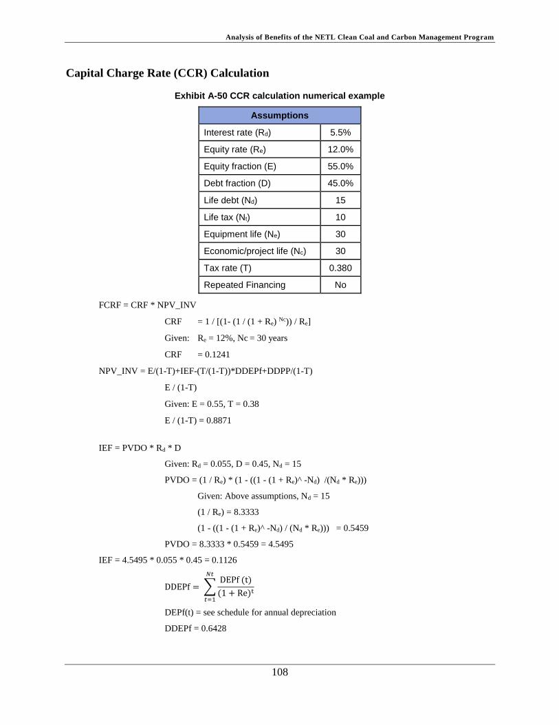
Analysis of Benefits of the NETL Clean Coal and Carbon Management Program
108
Capital Charge Rate (CCR) Calculation
Exhibit A-50 CCR calculation numerical example
Assumptions
Interest rate (Rd) 5.5%
Equity rate (Re) 12.0%
Equity fraction (E) 55.0%
Debt fraction (D) 45.0%
Life debt (Nd) 15
Life tax (Nt) 10
Equipment life (Ne) 30
Economic/project life (Nc) 30
Tax rate (T) 0.380
Repeated Financing No
FCRF = CRF * NPV_INV
CRF = 1 / [(1- (1 / (1 + Re) Nc)) / Re]
Given: Re = 12%, Nc = 30 years
CRF = 0.1241
NPV_INV = E/(1-T)+IEF-(T/(1-T))*DDEPf+DDPP/(1-T)
E / (1-T)
Given: E = 0.55, T = 0.38
E / (1-T) = 0.8871
IEF = PVDO * Rd * D
Given: Rd = 0.055, D = 0.45, Nd = 15
PVDO = (1 / Re) * (1 - ((1 - (1 + Re)^ -Nd) /(Nd * Re)))
Given: Above assumptions, Nd = 15
(1 / Re) = 8.3333
(1 - ((1 - (1 + Re)^ -Nd) / (Nd * Re))) = 0.5459
PVDO = 8.3333 * 0.5459 = 4.5495
IEF = 4.5495 * 0.055 * 0.45 = 0.1126
DDEPf = ∑DEPf (t)
(1 + Re)t
𝑁𝑡
𝑡=1
DEPf(t) = see schedule for annual depreciation
DDEPf = 0.6428

Analysis of Benefits of the NETL Clean Coal and Carbon Management Program
109
DDPP = ∑DPP (t)
(1 + Re)t
𝑁𝑑
𝑡=1
DPP(t) = see schedule for annual principal payments
DDPP = 0.2043
NPV_INV = 0.8871 + 0.1126 - 0.38/(1-0.38)*0.6428 + 0.2043/(1-0.38) = 0.9353
FCRF = CRF * NPV_INV = 0.1241 * 0.9353 = 0.1161
Exhibit A-51 Schedule of tax depreciation assuming double declining balance method changing over to straight line; debt principal payments
Year
Double Declining Balance
Debt
Depreciation Principal
1 0.2000 0.03
2 0.1600 0.03
3 0.1280 0.03
4 0.1024 0.03
5 0.0819 0.03
6 0.0655 0.03
7 0.0655 0.03
8 0.0655 0.03
9 0.0655 0.03
10 0.0655 0.03
11 0.03
12 0.03
13 0.03
14 0.03
15 0.03
Adjustments for Repeating Investments
If investments have to be repeated during the economic life of a project, then three of the
equations included in the prior FCRF formulation need adjustment. This adjustment accounts for
the out year financings associated with the investments.
The adjustment formula accounts for the number of additional infusions of financing (Nf) during
the economic life of the project excluding the initial pre-operational infusion.
If economic life (Econ Life) divided by equipment life (Equip Life) is an integer then Nf =
maximum of (Econ Life/Equip Life) - 1 and 0. To account for the initial round of financing, 1 is
subtracted.
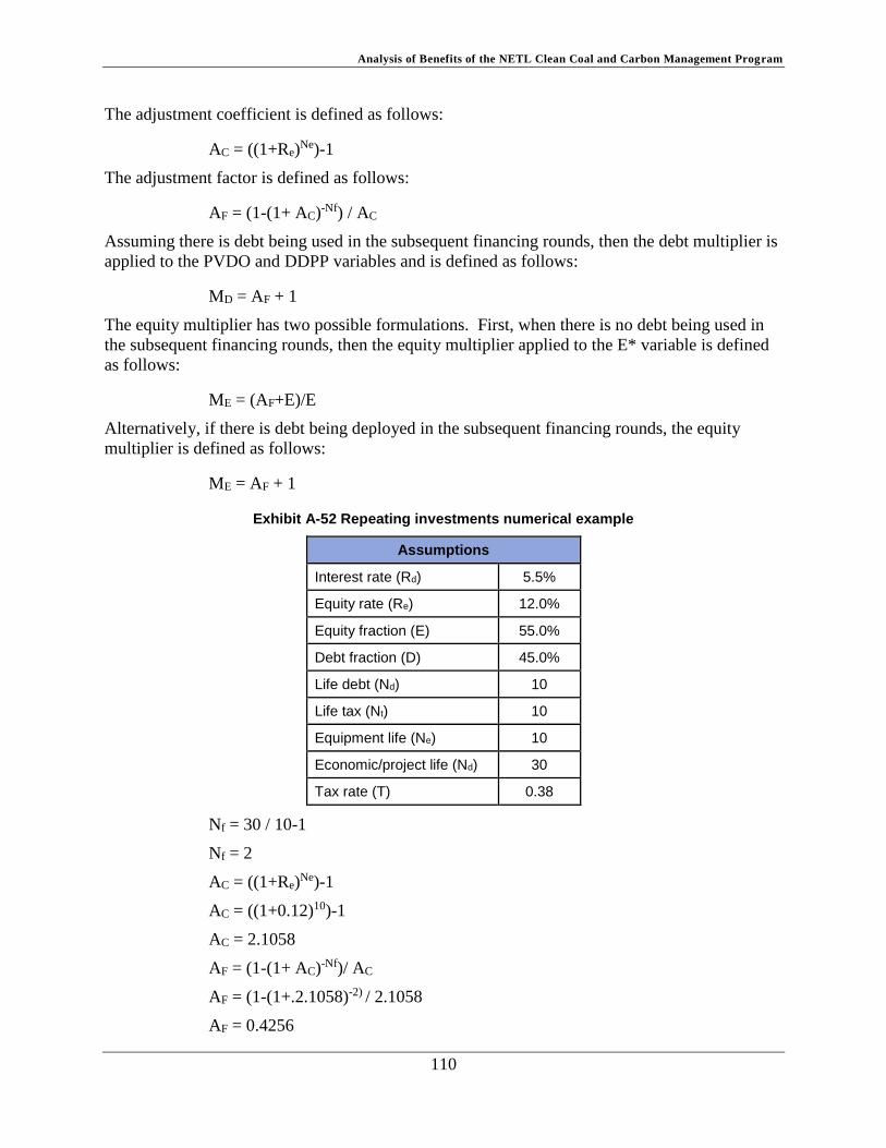
Analysis of Benefits of the NETL Clean Coal and Carbon Management Program
110
The adjustment coefficient is defined as follows:
AC = ((1+Re)Ne)-1
The adjustment factor is defined as follows:
AF = (1-(1+ AC)-Nf) / AC
Assuming there is debt being used in the subsequent financing rounds, then the debt multiplier is
applied to the PVDO and DDPP variables and is defined as follows:
MD = AF + 1
The equity multiplier has two possible formulations. First, when there is no debt being used in
the subsequent financing rounds, then the equity multiplier applied to the E* variable is defined
as follows:
ME = (AF+E)/E
Alternatively, if there is debt being deployed in the subsequent financing rounds, the equity
multiplier is defined as follows:
ME = AF + 1
Exhibit A-52 Repeating investments numerical example
Assumptions
Interest rate (Rd) 5.5%
Equity rate (Re) 12.0%
Equity fraction (E) 55.0%
Debt fraction (D) 45.0%
Life debt (Nd) 10
Life tax (Nt) 10
Equipment life (Ne) 10
Economic/project life (Nd) 30
Tax rate (T) 0.38
Nf = 30 / 10-1
Nf = 2
AC = ((1+Re)Ne)-1
AC = ((1+0.12)10)-1
AC = 2.1058
AF = (1-(1+ AC)-Nf)/ AC
AF = (1-(1+.2.1058)-2) / 2.1058
AF = 0.4256
Analysis of Benefits of the NETL Clean Coal and Carbon Management Program
111
Assuming there is debt used in subsequent financing:
MD = AF + 1
MD= 1.4256
Otherwise,
MD = 1.0
Assuming there is debt used in subsequent financing:
ME = AF + 1
ME = 1.4256
Otherwise,
ME= (AF+E)/E
ME = (0.4256+0.55)/0.55
ME = 1.7739
Multiplier to Account for Escalation during Construction/Interest during
Construction
Before applying the FCRF, the capital cost needs to be adjusted to account for escalation during
construction (EDC) and for interest during construction (IDC). Assuming cash is borrowed and
expended at the beginning of each year, the impact of EDC/IDC can be estimated using the
following:
𝐶𝐴𝐹 = ∑ 𝐶𝐹(𝑖) × (1 + 𝑒𝑠𝑐)𝑗−1
𝑥
𝑗=1
× (1 + 𝑖)(𝑥−𝑗+1)
(eq. 12)
Where:
CAF = capital cost adjustment factor (unitless)
CF(i) = fraction of bare costs expended in year j (unitless)
esc = escalation rate during construction (unitless)
i = construction period borrowing costs (unitless)
x = total number of years during construction
j = year
The following table highlights the impact of alternative assumptions on the calculation of CAF. It
assumes cash borrowed and spent at the beginning of the year.
Construction period borrowing costs (i) = 7.50%
Escalation during construction (esc) = 3.00%

Analysis of Benefits of the NETL Clean Coal and Carbon Management Program
112
Exhibit A-53 Impact of alternative assumptions
Construction Year (j)
% of Bare Costs
Profile 6 x = 1
Profile 5 x = 2
Profile 1 x = 3
Profile 2 x = 4
Profile 3 x = 5
Profile 4 x = 6
1 100% 25% 25% 10% 3% 3%
2 75% 50% 30% 9% 9%
3 25% 40% 30% 20%
4 20% 40% 30%
5 18% 30%
6 8%
7
Total % 100% 100% 100% 100% 100% 100%
EDC/IDC Multiplier
End of Year Convention
1.0750 1.1193 1.1908 1.2428 1.2852 1.3599
Mid-Year Convention
1.0523 1.0957 1.1656 1.2165 1.2580 1.3311
Periodic Investments Lasting Remaining Life
There is a type of recurring investment that presents a challenge to estimate its annualized costs.
When a project incurs periodic investment requirements that put in place assets that will last for
the economic life of the project, then a special approach needs to be taken to estimate the
equivalent annual cost that will yield an estimate of the capital carrying cost of these
investments.
For example, assume a project needs to invest a given amount every five years over its 30-year
life, i.e., in years 1, 6, 11, 16, 21, and 26. As stated above, these investments are assumed to
provide service over the remaining life of the project; year 1 investment has a 30-year life, year 6
investment has a 25-year life, etc. In these circumstances, using the algorithm described, the
CCR can be calculated for each of these investments. See Exhibit A-54 along with the additional
assumptions required shown in Exhibit A-55 and Exhibit A-56.
Exhibit A-54 Periodic investments (years)
Inservice year 1 6 11 16 21 26
Life debt (Nd) 15 15 15 15 10* 5*
Life tax (Nt) 5 5 5 5 5 5
Equipment life (Ne) 30 25 20 15 10* 5*
Economic/project life (Nc) 30 25 20 15 10* 5*
* The debt life and equipment life are adjusted to not go past the end of the project life.

Analysis of Benefits of the NETL Clean Coal and Carbon Management Program
113
Exhibit A-55 Periodic investments numerical example
Assumptions
Interest rate (Rd) 5.5%
Equity rate (Re) 12.0%
Equity fraction (E) 55.0%
Debt fraction (D) 45.0%
Tax rate (T) 0.38
Exhibit A-56 Periodic investments
Inservice year 1 6 11 16 21 26
Calculated CCR* 0.1056 0.1085 0.1139 0.1249 0.1608 0.2744
Present worth factor 1.000 0.5674 0.3220 0.1827 0.1037 0.0588
* These values were calculated using the methodology illustrated in Appendix A.8: Financial Functions in CO2 CTUS-NEMS.
Since these investments are spread out over the life, in order to calculate the equivalent annual
cost, the investments need to be discounted back to the beginning of the project. Calculating the
sum product of the CCR and the present worth factors gives 0.2595. This is the CCR applied to
1/6 of the PV of the periodic investments.
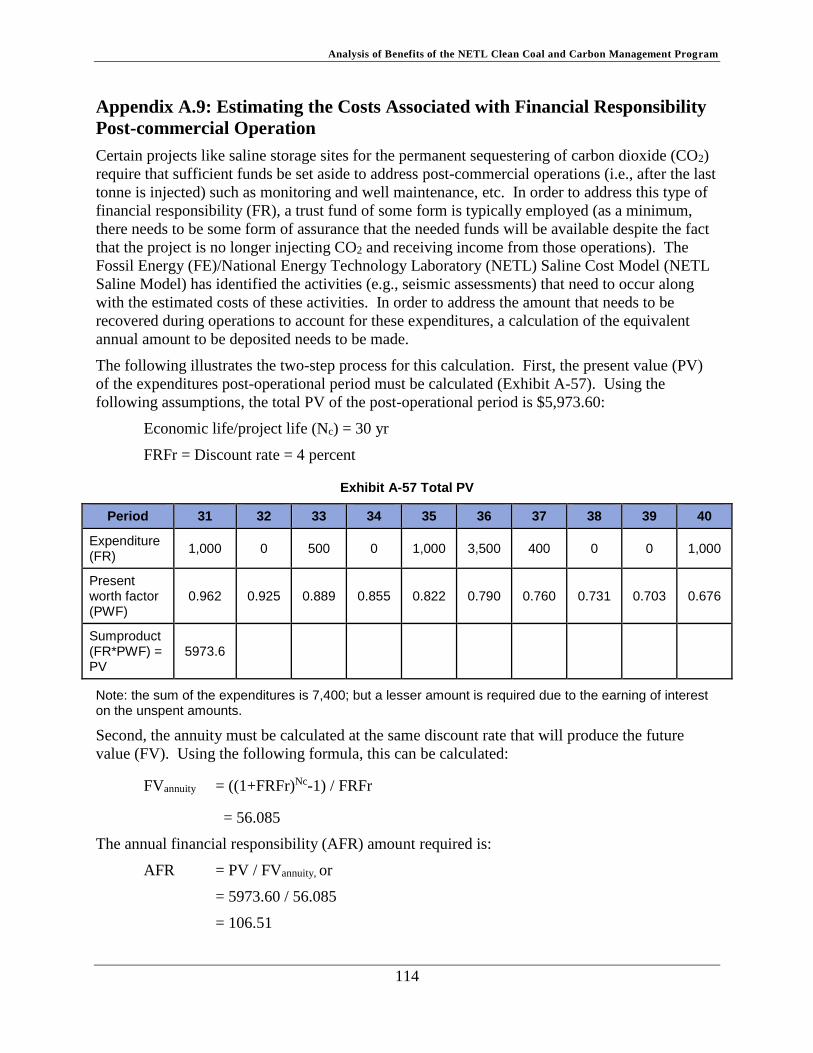
Analysis of Benefits of the NETL Clean Coal and Carbon Management Program
114
Appendix A.9: Estimating the Costs Associated with Financial Responsibility
Post-commercial Operation
Certain projects like saline storage sites for the permanent sequestering of carbon dioxide (CO2)
require that sufficient funds be set aside to address post-commercial operations (i.e., after the last
tonne is injected) such as monitoring and well maintenance, etc. In order to address this type of
financial responsibility (FR), a trust fund of some form is typically employed (as a minimum,
there needs to be some form of assurance that the needed funds will be available despite the fact
that the project is no longer injecting CO2 and receiving income from those operations). The
Fossil Energy (FE)/National Energy Technology Laboratory (NETL) Saline Cost Model (NETL
Saline Model) has identified the activities (e.g., seismic assessments) that need to occur along
with the estimated costs of these activities. In order to address the amount that needs to be
recovered during operations to account for these expenditures, a calculation of the equivalent
annual amount to be deposited needs to be made.
The following illustrates the two-step process for this calculation. First, the present value (PV)
of the expenditures post-operational period must be calculated (Exhibit A-57). Using the
following assumptions, the total PV of the post-operational period is $5,973.60:
Economic life/project life (Nc) = 30 yr
FRFr = Discount rate = 4 percent
Exhibit A-57 Total PV
Period 31 32 33 34 35 36 37 38 39 40
Expenditure (FR)
1,000 0 500 0 1,000 3,500 400 0 0 1,000
Present worth factor (PWF)
0.962 0.925 0.889 0.855 0.822 0.790 0.760 0.731 0.703 0.676
Sumproduct (FR*PWF) = PV
5973.6
Note: the sum of the expenditures is 7,400; but a lesser amount is required due to the earning of interest on the unspent amounts.
Second, the annuity must be calculated at the same discount rate that will produce the future
value (FV). Using the following formula, this can be calculated:
FVannuity = ((1+FRFr)Nc-1) / FRFr
= 56.085
The annual financial responsibility (AFR) amount required is:
AFR = PV / FVannuity, or
= 5973.60 / 56.085
= 106.51
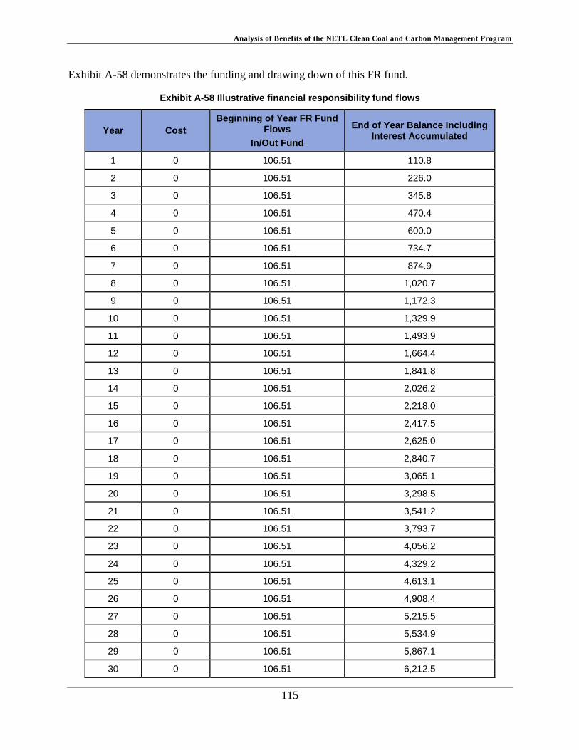
Analysis of Benefits of the NETL Clean Coal and Carbon Management Program
115
Exhibit A-58 demonstrates the funding and drawing down of this FR fund.
Exhibit A-58 Illustrative financial responsibility fund flows
Year Cost
Beginning of Year FR Fund Flows
In/Out Fund
End of Year Balance Including Interest Accumulated
1 0 106.51 110.8
2 0 106.51 226.0
3 0 106.51 345.8
4 0 106.51 470.4
5 0 106.51 600.0
6 0 106.51 734.7
7 0 106.51 874.9
8 0 106.51 1,020.7
9 0 106.51 1,172.3
10 0 106.51 1,329.9
11 0 106.51 1,493.9
12 0 106.51 1,664.4
13 0 106.51 1,841.8
14 0 106.51 2,026.2
15 0 106.51 2,218.0
16 0 106.51 2,417.5
17 0 106.51 2,625.0
18 0 106.51 2,840.7
19 0 106.51 3,065.1
20 0 106.51 3,298.5
21 0 106.51 3,541.2
22 0 106.51 3,793.7
23 0 106.51 4,056.2
24 0 106.51 4,329.2
25 0 106.51 4,613.1
26 0 106.51 4,908.4
27 0 106.51 5,215.5
28 0 106.51 5,534.9
29 0 106.51 5,867.1
30 0 106.51 6,212.5
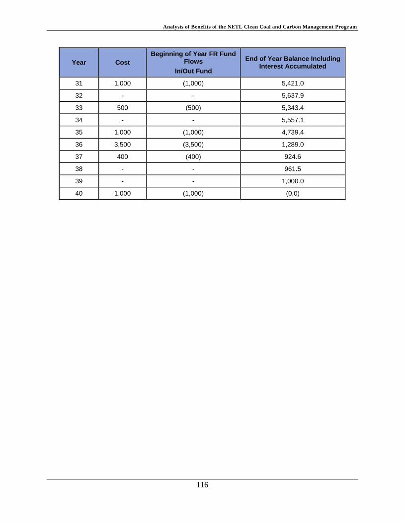
Analysis of Benefits of the NETL Clean Coal and Carbon Management Program
116
Year Cost
Beginning of Year FR Fund Flows
In/Out Fund
End of Year Balance Including Interest Accumulated
31 1,000 (1,000) 5,421.0
32 - - 5,637.9
33 500 (500) 5,343.4
34 - - 5,557.1
35 1,000 (1,000) 4,739.4
36 3,500 (3,500) 1,289.0
37 400 (400) 924.6
38 - - 961.5
39 - - 1,000.0
40 1,000 (1,000) (0.0)

Analysis of Benefits of the NETL Clean Coal and Carbon Management Program
117
Appendix B: Econometric Input-Output Model Overview
Appendix B.1: Introduction
This document provides an overview of the National Energy Technology Laboratory (NETL)/
West Virginia University (WVU) Econometric Input-Output (ECIO) model, a time-series
enabled hybrid econometric input-output (IO) model that combines the capabilities of
econometric modeling with the strengths of IO modeling. It is designed to facilitate the
estimation of economic (specifically, employment and income) impacts of energy technology
development, deployment, and operation over a forecast period consistent with the National
Energy Modeling System (NEMS), providing a consistent and comprehensive method for
quantifying NETL’s programmatic impacts.
The NETL/WVU ECIO model (hereafter, ECIO model) integrates a macroeconomic forecasting
model of the United States (U.S.) economy with an interindustry accounting framework that
characterizes the interdependence of industries, value added sectors, and final demands through
sales and purchases. The model consists of three modules and several sub-modules of
interrelated equations that represent the U.S. economy and/or industry level details for 32
industrial sectors. The three major modules are:
1. Fair model: a macroeconomic econometric model of the U.S.
2. Industrial output module
3. Employment module
Using the baseline data defined during model design and database development, the national
ECIO model can be used to estimate the economic impacts of a baseline technology deployment
profile. At this stage of its development, the macroeconomic model has been fully integrated
with the interindustry model (IO) module. Further development focuses on continued refinement
of model equations and the transcription of NEMS model output into scenarios. With complete
scenario description data sets in place, the model can be applied to the estimation of economic
and employment impacts of new energy technologies.
The purpose of this document is to provide an overview report on the ECIO model to serve as a
reference document for the June 2016 version of the model. Appendix B.2: Model Design
provides an overview of the model design and the general assumptions associated with the ECIO
model. Appendix B.3: Input Data describes the input data requirements and Appendix B.4:
Model Outputs discusses the regional capabilities of the ECIO model. Appendix B.5: Equations
and Variables of the Macroeconomic Econometric Module provides a brief discussion of the
model outputs.
An Operator’s Manual for the June 2016 version of the ECIO model is available as a separate
document and contains details associated with the actual implementation of the model.

Analysis of Benefits of the NETL Clean Coal and Carbon Management Program
118
Appendix B.2: Model Design
The ECIO model integrates a macroeconomic econometric forecasting framework that represents
the entire U.S. economy with an input-output framework that reflects the interindustry
interdependence within the U.S. economy. The ECIO model has three modules and several
submodules of interrelated equations representing the entire U.S. economy, which is modeled as
consisting of 32 industrial sectors. The three major modules are the Fair U.S. macroeconomic
econometric model, the industrial output module, and the employment module, shown in Exhibit
B-1.
Exhibit B-1 ECIO model configuration
Macroeconomic Econometric Module
The Fair model, a macroeconomic econometric model developed by Ray Fair (2004), is used to
forecast values related to the size of the overall U.S. economy. The Fair model captures the
interdependence and interactions among the six major components of the U.S. economy:
households (h), firms (b), financials (f), international component (r), federal government (g), and
state governments (s). This model provides a theoretical framework for the projections while

Analysis of Benefits of the NETL Clean Coal and Carbon Management Program
119
maintaining a balance among different economic variables. The quarterly model comprises 289
variables (147 endogenous and 142 exogenous variables) in 128 equations (26 stochastic and 102
identities) that describe the U.S. economy. Most of the stochastic equations are estimated via the
Two Stage Least Squares method. Most estimated equations include a lagged dependent variable
as an explanatory variable to account for both partial adjustment and expectation effects. The key
outputs of the model are the forecasts of the components of final demand that serve as inputs to
the industrial output module (the IO component of the overall model). Gross final demand
components of consumption, investment, imports, exports, and government expenditures are all
estimated in a consistent manner. A bridge matrix based on the most recent BEA benchmark IO
tables is used to transform the forecasted aggregate components of final demand into demand by
commodity. The following sections detail the construction of each of the final demand
components within the ECIO model, the determination of gross domestic product within the
Macroeconomic Econometric module, and the estimation of total private production and total
employment within the ECIO model. A complete description of all the variables and equations
used in the Macroeconomic Econometric Module is found in Appendix B.5: Equations and
Variables of the Macroeconomic Econometric Module.
Final Demand Components
Consumption Expenditures
The household consumption component within the Fair model consists of four consumption
categories including consumption of services (CS), durable goods (CD), nondurable goods (CN),
and residential investment (IHH). This aggregation is modified in two ways within the ECIO
model. First, the categories representing the consumption of services, durable goods, and
nondurable goods were partially disaggregated to create four additional consumption categories:
gasoline, motor vehicles and parts, natural gas, and electricity. Next, the residential investment
category was moved into the investment component of final demand. The seven resulting
consumption expenditure categories within the Macroeconomic Econometric Module are:
1. Motor vehicles and parts
2. Gasoline
3. Electricity
4. Other durable goods
5. Other nondurable goods
6. Natural Gas
7. Other services
The key determinants of personal consumption expenditure on commodity i (Ci) are current
disposable income (YD), past total net wealth (AAt-1), past consumption (Ct-1), the price deflator
of consumption (PH), the interest rate (R), the age distribution of the population (AGi), total
population (POP), and a time trend (t). With the exception of age distribution variables that are
exogenous, these variables are endogenously determined within the model. A representative
form of the consumption equation is shown in equation 1.
(1) 𝐿𝑜𝑔 (𝐶𝑖
𝑃𝑂𝑃) = 𝑓 (𝐴𝐺1, 𝐴𝐺2, 𝐴𝐺3, 𝐿𝑜𝑔 (
𝐶𝑖
𝑃𝑂𝑃)
𝑡−1, 𝐿𝑜𝑔 (
𝐴𝐴
𝑃𝑂𝑃)
𝑡−1, 𝐿𝑜𝑔 (
𝑌𝐷
𝑃𝑂𝑃 ∗ 𝑃𝐻) , 𝑅𝑖, 𝑡)

Analysis of Benefits of the NETL Clean Coal and Carbon Management Program
120
Investment
Private investment comprises residential investment (IHH, IHB, IHF), nonresidential fixed
investment (IKH, IKB, IKF), and inventory investment (IVF). The seven investment variables
determine the flow of private investment from the household (h), firm (b), and financial (f)
sectors to the economy. With the exception of household residential investment (IHH), financial
sector nonresidential fixed investment (IKF), and financial sector inventory investment (IVF),
the investment variables are exogenously determined outside of the ECIO model. The
specifications of the three behavioral equations in the investment sub module are as follows:
(2) ∆𝐼𝐻𝐻
𝑃𝑂𝑃= 𝑓 (𝐷𝐸𝐿𝐻 (
𝐾𝐻
𝑃𝑂𝑃)
𝑡−1− (
𝐼𝐻𝐻
𝑃𝑂𝑃)
𝑡−1, (
𝐾𝐻
𝑃𝑂𝑃)
𝑡−1, (
𝐴𝐴
𝑃𝑂𝑃)
𝑡−1, (
𝑌𝐷
𝑃𝑂𝑃 ∗ 𝑃𝐻) , 𝑅𝑀𝐴𝑡−1
(3) 𝐼𝐾𝐹 = 𝐾𝐾 − (1 − 𝐷𝐸𝐿𝐾)𝐾𝐾𝑡−1
(4) 𝐼𝑉𝐹 = 𝑉 − 𝑉𝑡−1
The variable KH is housing stock, DELH is depreciation rate of housing stock, KK is stock of
capital, DELK is the physical depreciation rate of the stock of capital, IHH is Residential
investment, RMA is mortgage interest rate, V is stock of inventory and IHH, AA, YD are defined
as in the consumption equation.
Government Expenditure
There are two types of government expenditures in the model: federal and state government
(COG and COS) consumption and investment goods purchases, and nonresidential fixed
investment by the government sector (IKG). All three of these variables are exogenously
determined.
Net Exports
Exports (EX) and export growth rates are exogenous in the Fair model. Imports (IM) are
determined endogenously as a function of consumption and investment spending, the domestic
price level (PF), the import price level (PIM), and time-dependent dummy variables (Di). The
form of the imports function is shown in equation 5.
(5) 𝐿𝑜𝑔 (𝐼𝑀
𝑃𝑂𝑃) = 𝑓((
𝐼𝑀
𝑃𝑂𝑃)
𝑡−1, 𝐿𝑂𝐺 [
𝐶𝑆+𝐶𝑁+𝐶𝐷+𝐼𝐻𝐻+𝐼𝐻𝐵+𝐼𝐻𝐹+𝐼𝐾𝐻+𝐼𝐾𝐵+𝐼𝐾𝐹
𝑃𝑂𝑃] , 𝐿𝑂𝐺 (
𝑃𝐹
𝑃𝐼𝑀) , 𝐷𝑖
GDP Determination in the Fair Model
By definition, GDP is equal to consumption plus investment plus government spending plus
exports minus imports. In the Fair model, the six sectors (households [h], firms [b], financials [f], international [r], federal government
[g], and local government, [s]) – in addition to a number of categories of consumption, investment, and
government spending – result in a more complex restatement of GDP. Real gross domestic
product (GDPR) is defined here as the sum of business production (Y = consumption +
investment + government spending + net export), production of the financial sector (capital
consumption [CCB], + before tax profits, [PIEB]), and government sector production (federal
civilian [JG*HG], and military [JM*HM], and state [JS*HS]) compensation of civilian and
military employees). JG, JM, and JS are the number of civilian, military, and state jobs
respectively. HG, HM, HS are the average number of hours paid per civilian, military, and state
job respectively. The resulting gross product equation (6) is shown below.
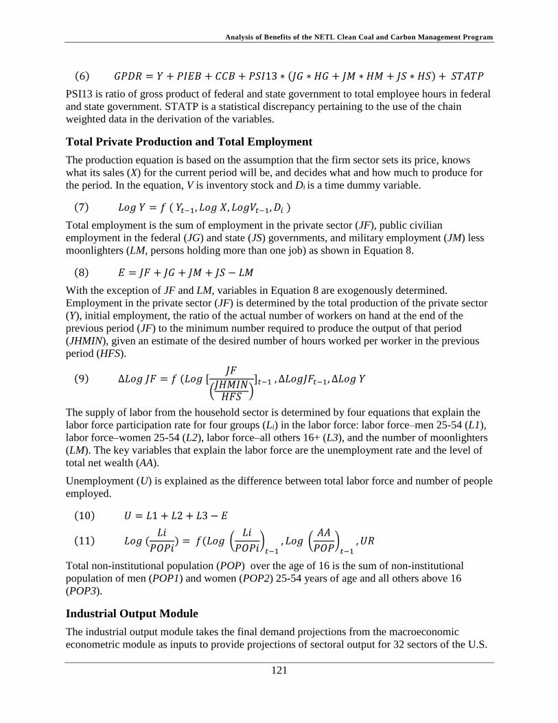
Analysis of Benefits of the NETL Clean Coal and Carbon Management Program
121
(6) 𝐺𝑃𝐷𝑅 = 𝑌 + 𝑃𝐼𝐸𝐵 + 𝐶𝐶𝐵 + 𝑃𝑆𝐼13 ∗ (𝐽𝐺 ∗ 𝐻𝐺 + 𝐽𝑀 ∗ 𝐻𝑀 + 𝐽𝑆 ∗ 𝐻𝑆) + 𝑆𝑇𝐴𝑇𝑃
PSI13 is ratio of gross product of federal and state government to total employee hours in federal
and state government. STATP is a statistical discrepancy pertaining to the use of the chain
weighted data in the derivation of the variables.
Total Private Production and Total Employment
The production equation is based on the assumption that the firm sector sets its price, knows
what its sales (X) for the current period will be, and decides what and how much to produce for
the period. In the equation, V is inventory stock and Di is a time dummy variable.
(7) 𝐿𝑜𝑔 𝑌 = 𝑓 ( 𝑌𝑡−1, 𝐿𝑜𝑔 𝑋, 𝐿𝑜𝑔𝑉𝑡−1, 𝐷𝑖 )
Total employment is the sum of employment in the private sector (JF), public civilian
employment in the federal (JG) and state (JS) governments, and military employment (JM) less
moonlighters (LM, persons holding more than one job) as shown in Equation 8.
(8) 𝐸 = 𝐽𝐹 + 𝐽𝐺 + 𝐽𝑀 + 𝐽𝑆 − 𝐿𝑀
With the exception of JF and LM, variables in Equation 8 are exogenously determined.
Employment in the private sector (JF) is determined by the total production of the private sector
(Y), initial employment, the ratio of the actual number of workers on hand at the end of the
previous period (JF) to the minimum number required to produce the output of that period
(JHMIN), given an estimate of the desired number of hours worked per worker in the previous
period (HFS).
(9) ∆𝐿𝑜𝑔 𝐽𝐹 = 𝑓 (𝐿𝑜𝑔 [𝐽𝐹
(𝐽𝐻𝑀𝐼𝑁
𝐻𝐹𝑆 )]𝑡−1 , ∆𝐿𝑜𝑔𝐽𝐹𝑡−1, ∆𝐿𝑜𝑔 𝑌
The supply of labor from the household sector is determined by four equations that explain the
labor force participation rate for four groups (Li) in the labor force: labor force–men 25-54 (L1),
labor force–women 25-54 (L2), labor force–all others 16+ (L3), and the number of moonlighters
(LM). The key variables that explain the labor force are the unemployment rate and the level of
total net wealth (AA).
Unemployment (U) is explained as the difference between total labor force and number of people
employed.
(10) 𝑈 = 𝐿1 + 𝐿2 + 𝐿3 − 𝐸
(11) 𝐿𝑜𝑔 (𝐿𝑖
𝑃𝑂𝑃𝑖) = 𝑓(𝐿𝑜𝑔 (
𝐿𝑖
𝑃𝑂𝑃𝑖)
𝑡−1, 𝐿𝑜𝑔 (
𝐴𝐴
𝑃𝑂𝑃)
𝑡−1, 𝑈𝑅
Total non-institutional population (POP) over the age of 16 is the sum of non-institutional
population of men (POP1) and women (POP2) 25-54 years of age and all others above 16
(POP3).
Industrial Output Module
The industrial output module takes the final demand projections from the macroeconomic
econometric module as inputs to provide projections of sectoral output for 32 sectors of the U.S.
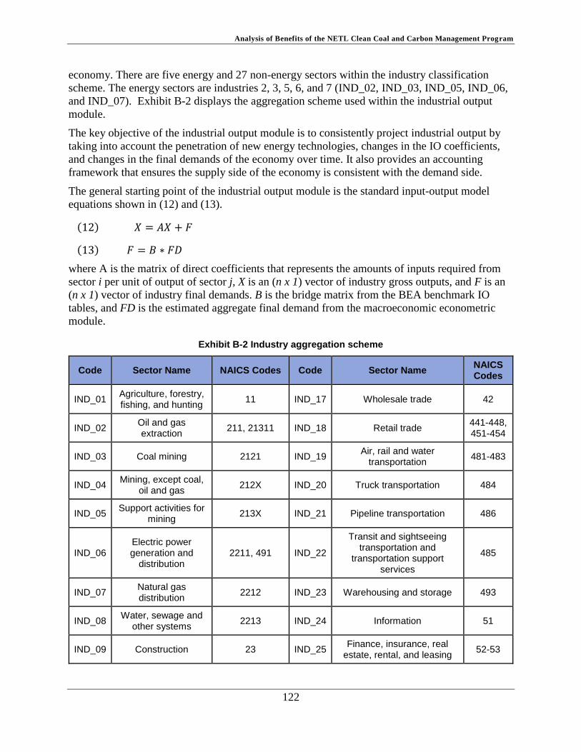
Analysis of Benefits of the NETL Clean Coal and Carbon Management Program
122
economy. There are five energy and 27 non-energy sectors within the industry classification
scheme. The energy sectors are industries 2, 3, 5, 6, and 7 (IND_02, IND_03, IND_05, IND_06,
and IND_07). Exhibit B-2 displays the aggregation scheme used within the industrial output
module.
The key objective of the industrial output module is to consistently project industrial output by
taking into account the penetration of new energy technologies, changes in the IO coefficients,
and changes in the final demands of the economy over time. It also provides an accounting
framework that ensures the supply side of the economy is consistent with the demand side.
The general starting point of the industrial output module is the standard input-output model
equations shown in (12) and (13).
(12) 𝑋 = 𝐴𝑋 + 𝐹
(13) 𝐹 = 𝐵 ∗ 𝐹𝐷
where A is the matrix of direct coefficients that represents the amounts of inputs required from
sector i per unit of output of sector j, X is an (n x 1) vector of industry gross outputs, and F is an
(n x 1) vector of industry final demands. B is the bridge matrix from the BEA benchmark IO
tables, and FD is the estimated aggregate final demand from the macroeconomic econometric
module.
Exhibit B-2 Industry aggregation scheme
Code Sector Name NAICS Codes Code Sector Name NAICS Codes
IND_01 Agriculture, forestry, fishing, and hunting
11 IND_17 Wholesale trade 42
IND_02 Oil and gas extraction
211, 21311 IND_18 Retail trade 441-448, 451-454
IND_03 Coal mining 2121 IND_19 Air, rail and water
transportation 481-483
IND_04 Mining, except coal,
oil and gas 212X IND_20 Truck transportation 484
IND_05 Support activities for
mining 213X IND_21 Pipeline transportation 486
IND_06 Electric power generation and
distribution 2211, 491 IND_22
Transit and sightseeing transportation and
transportation support services
485
IND_07 Natural gas distribution
2212 IND_23 Warehousing and storage 493
IND_08 Water, sewage and
other systems 2213 IND_24 Information 51
IND_09 Construction 23 IND_25 Finance, insurance, real
estate, rental, and leasing 52-53
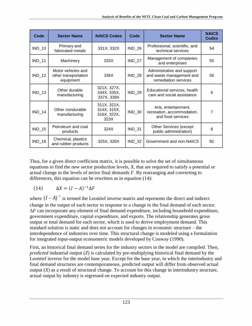
Analysis of Benefits of the NETL Clean Coal and Carbon Management Program
123
Code Sector Name NAICS Codes Code Sector Name NAICS Codes
IND_10 Primary and
fabricated metals 331X, 332X IND_26
Professional, scientific, and technical services
54
IND_11 Machinery 333X IND_27 Management of companies
and enterprises 55
IND_12 Motor vehicles and other transportation
equipment 336X IND_28
Administrative and support and waste management and
remediation services 56
IND_13 Other durable manufacturing
321X, 327X, 334X, 335X, 337X, 339X
IND_29 Educational services, health care and social assistance
6
IND_14 Other nondurable
manufacturing
311X, 321X, 314X, 315X, 316X, 322X,
323X
IND_30 Arts, entertainment,
recreation, accommodation, and food services
7
IND_15 Petroleum and coal
products 324X IND_31
Other Services (except public administration)
8
IND_16 Chemical, plastics
and rubber products 325X, 326X IND_32 Government and non-NAICS 92
Thus, for a given direct coefficient matrix, it is possible to solve the set of simultaneous
equations to find the new sector production levels, X, that are required to satisfy a potential or
actual change in the levels of sector final demands F. By rearranging and converting to
differences, this equation can be rewritten as in equation (14):
(14) ∆𝑋 = (𝐼 − 𝐴)−1∆𝐹
where 1)( AI is termed the Leontief inverse matrix and represents the direct and indirect
change in the output of each sector in response to a change in the final demand of each sector.
ΔF can incorporate any element of final demand expenditure, including household expenditure,
government expenditure, capital expenditure, and exports. The relationship generates gross
output or total demand for each sector, which is used to derive employment demand. This
standard solution is static and does not account for changes in economic structure – the
interdependence of industries over time. This structural change is modeled using a formulation
for integrated input-output econometric models developed by Conway (1990).
First, an historical final demand series for the industry sectors in the model are compiled. Then,
predicted industrial output (Z) is calculated by pre-multiplying historical final demand by the
Leontief inverse for the model base year. Except for the base year, in which the interindustry and
final demand structures are contemporaneous, predicted output will differ from observed actual
output (X) as a result of structural change. To account for this change in interindustry structure,
actual output by industry is regressed on expected industry output.
Analysis of Benefits of the NETL Clean Coal and Carbon Management Program
124
(15) 𝑋 = 𝑓(𝑍, 𝑀)
where M, when it is present, includes a set of related independent variables that help explain the
change in IO coefficients for each sector. Actual output will be revealed to be growing more
slowly or quickly than predicted output. As the model forecast progresses, the output response to
forecast final demand for each industry is adjusted by this relationship between actual and
predicted output.
Industrial Employment Module
The industrial employment module uses the industrial output (Xi) projections from the industrial
output module, average national wage rates (AWUS), industrial labor productivity (INDPi) trends,
and initial industrial employment (INDEi) to project employment for the 32 industries.
(16) 𝐿𝑜𝑔 𝐼𝑁𝐷𝐸𝑖 = 𝑓( 𝐴𝑊𝑈𝑆 , 𝐿𝑜𝑔 𝐼𝑁𝐷𝑃𝑖 , 𝑋𝑖 ,𝐿𝑜𝑔 𝐼𝑁𝐷𝐸𝑖,𝑡−1 )
Total industrial employment (INDE) at time t is the sum of all employed persons in all the
sectors at time t.
(17) 𝐼𝑁𝐷𝐸𝑡 = ∑ 𝐼𝑁𝐷𝐸𝑖
Trends in average wage rates and in productivities by industry are forecast econometrically.
Output forecasts by industry combined with labor productivities determine employment by
industry, which when combined with wage rate estimates determine the production labor income
portion of household income.
This total labor income together with non-labor income is used to update disposable income
(YD), which is a major driver of consumption expenditure in the macroeconomic econometric
module.
Notable Model Capabilities
Power Sector Updates
The ECIO model is able to adapt to and incorporate updates to the aggregated electricity
generation, transmission, and distribution sector (IND_06) based on scenario specific input data
from NEMS. Specifically, annual Use tables within the Industrial Output Module are updated to
reflect scenario specific information on how the technology mix within the electricity generation
sector changes over the forecast period. Scenario specific information is provided via the NETL
NEMS-ECIO Translation Tool. Details on the data involved and the translation process can be
found in the NETL NEMS-ECIO Translation Tool: Model Overview Report.
Price Flexibility
The model allows for and responds to changes in energy sector prices. Normally, these energy
sector price changes are obtained from the NEMS model output and are used as inputs to the
ECIO model. As energy prices change, production costs to other industries also change,
resulting in further production cost changes to all industries. These direct and indirect price
effects are incorporated in the ECIO model using a variant of the input-output price model.
Although prices of all goods change, no input substitution behavior is modeled.

Analysis of Benefits of the NETL Clean Coal and Carbon Management Program
125
Integration Mechanisms
There are two primary mechanisms that integrate the interindustry and econometric subsystems.
The first of these is the reliance of the interindustry output requirements solution on econometric
final demand estimates. Final demand totals by activity (e.g., consumption, government
expenditures, investment expenditures) are transformed using commodity final demand
distribution data from the national input-output accounts.
The second integrating mechanism focuses on income estimation. Because income is the source
of consumption expenditures and because consumption expenditures are the dominant driving
force and determinant of overall economic activity (i.e., GDP), income provides a powerful
location for integrating the two model systems. Econometric time series provide the basis for
forecast labor and non-labor income estimates, and production based output estimates coupled
with productivities and wage rates provide a second source for labor income estimates. The
model uses a variable weighting parameter in which full or partial weight can be accorded to
either the IO or econometric labor income estimate. By weighting the two equally, the
econometric and IO sub-systems exert equal influence on the initial impacts solutions for each
year. Because each model year is solved iteratively, the final weighting of econometric and IO
labor income estimates may deviate from the equal weighting, but the initial solution starting
point for each year allows equal influence of econometric and input-output estimates.
After the weighted combinations of non-labor income estimates are added to econometrically
estimated non-labor income, the total is converted to disposable income, which in turn drives
consumption.

Analysis of Benefits of the NETL Clean Coal and Carbon Management Program
126
Appendix B.3: Input Data
Each module of the ECIO model requires a foundation database that consists of time series and
cross section variables representing a variety of economic parameters. Additional scenario
specific data are normally drawn from National Energy Modeling System (NEMS) outputs. The
following sections provide additional detail on module specific data requirements with the three
ECIO modules as well as the scenario specific NEMS data made available through the NETL
NEMS-ECIO Translation Tool.
Macroeconomic Econometric Data
The foundation data of the Fair model are provided in Appendix B.5: Equations and Variables of
the Macroeconomic Econometric Module. These two files include all the variables and equations
of Fair model. The following two files, downloadable from
http://fairmodel.econ.yale.edu/eviews/eviews.htm, contain all of the Fair model data.
fm.wfl the fair model Eviews® data
yfair.prg reads the Eviews® data from “fm.wfl”
More complete descriptions of the variables are provided in Appendix B.5: Equations and
Variables of the Macroeconomic Econometric Module.
From the Fair model, 15 GDP components will be projected and serve as input to the industrial
output module (IO component of the overall model). The final demand components include three
consumption (durable, nondurable, and service), seven investment (three residential, three
nonresidential, and inventory investment), three categories of government expenditures, import
and export. The three consumption variables are disaggregated into seven consumption
expenditures: motor vehicles and parts, other durable goods, gasoline, other nondurable goods,
electricity, gas, and other services.
The Fair Model data for the current version of the model are the July 31, 2014 version, and
include
Quarterly data (1952:1 through 2012:4) for 377 variables (227 endogenous and 150
exogenous) that describe the U.S. economy
Fair model data sources include:
Bureau of Economic Analysis: National Income and Product Accounts (NIPA)
Bureau of Labor Statistics
Census Bureau
Board of Governors of the Federal Reserve
Industrial Output Module
The industrial output module uses two foundation datasets: IO data that consists of 32 aggregated
sectors and a time series dataset of industrial gross output.
Analysis of Benefits of the NETL Clean Coal and Carbon Management Program
127
Input-Output Data
Data used to construct the IO tables and final demand bridge matrix are drawn from the Bureau
of Labor Statistics (BLS) benchmark tables for 1993 to 2012. Data are reported for 195
commodity and 191 industry sectors, which are then further aggregated to the 32-sector level of
detail in Exhibit B-2. The online data descriptions, which can be found at
http://www.bls.gov/emp/ep_data_input_output_matrix.htm, and the primary downloadable file
found at http://www.bls.gov/emp/input-output/input-output.zip contains the following files used
in ECIO model construction:
FD 195 commodity rows and 191 detailed final demand sectors of data
FDAGG 195 commodity rows and 12 final demand categories of data aggregated from
the 191 sectors mentioned above
MAKE 195 rows and 195 columns of data
USE 196 rows and 196 columns of data (row 196 is value added; column 196 is final
demand; the rest are the intermediate cells)
OUTPUT_COM9312 1993-2012 historical commodity output time series (columns 1
through 20 respectively)
OUTPUT_IND9312 1993-2012 historical industry output time series (columns 1
through 20 respectively)
Industrial Gross Output
Data for industrial output are collected from the same source as input-output data, which is from
http://www.bls.gov/emp/ep_data_industry_out_and_emp.htm. The data file with link
http://www.bls.gov/emp/Industry-Employment/industry.zip includes:
ind12 industry output data from 1972 to 2012
Industrial Employment Module
The dataset used for this module includes an annual time series for employment, compensation
of employees, and labor productivity by industry.
Employment
The major data source of industrial employment is Bureau of Labor Statistics (BLS),
http://www.bls.gov/cew/datatoc.htm. The files used are labeled “Legacy Flat ENB/END” files.
Once downloaded, the “national” folders contain data on national employment by industry,
labeled:
NT00US(90-12).ENB: national employment data from 1990 to 2012
Compensation of Employees
The value of compensation of employees comes from the BEA tables, which is from
http://www.bea.gov/industry/gdpbyind_data.htm. The list of data files used in ECIO
development includes:
Analysis of Benefits of the NETL Clean Coal and Carbon Management Program
128
GDPbyInd_VA_NAICS_1947-1997: GDP by Industry data before 1997
GDPbyInd_VA_NAICS_1997-2013: GDP by Industry data after 1997
Industry_aggregate, industry_plan.m: aggregate the industries into 32 industries
Energy and Electricity Sector Data
The NEMS-ECIO Translation tool, housed within NETL, provides scenario specific data from
NEMS that are used to update energy related variables and the make-up of the electricity
generation sector within the ECIO model. The *.xls input file that is provided includes:
Average electricity price to all consumers
Average coal minemouth price
Composite average petroleum and natural gas price
Overnight capital costs by year and ECIO sector
Operation and maintenance expenditures by year and ECIO sector
Direct employment impacts by year, ECIO sector, and region
Direct income impacts by year, ECIO sector, and region
Electricity sales impact by year and region with breakdowns associated with technologies
that are within the scenario vs. outside of the scenario
National Enhanced Oil Recovery sales impact by year
National CO2 pipeline revenue by year
CO2 saline storage site revenue by year
CO2 tax revenue by year
Estimated technical coefficients for the “included technologies” portion of the aggregated
electricity generation sector
The definition and availability of the information within this input file will determine the
technologies and processes that are directly modeled, indirectly modeled, and/or not modeled by
the ECIO model.
Regional Capabilities
The ECIO model includes a mechanism for generating estimates of total impacts for a set of
subnational regions. Impacts regionalization occurs after the national impacts have been
generated, and only when the direct impacts being modeled are allocated to the subnational
regions. The regionalization mechanism then generates an estimate of total impacts by region by
weighting the impacts according to a combination of the distribution of direct impacts and the
distribution of all industrial employment in the U.S.
Regional Classification
The regional classification of the ECIO model follows the regional divisions used by the U.S.
Census Bureau since part of the regional impacts allocation procedure (indirect and induced

Analysis of Benefits of the NETL Clean Coal and Carbon Management Program
129
impacts) is a function of the existing regional distribution of employment by industry. States are
grouped into nine regional divisions as described in Exhibit B-3 and shown in Exhibit B-4.
Exhibit B-3 Definition of U.S. Census Bureau regions
Regions Name States
Region1 New England Connecticut (CT), Maine (ME), Massachusetts (MA), New Hampshire (NH), Rhode Island (RI), Vermont (VT)
Region 2 Mid Atlantic New Jersey (NJ), New York (NY), Pennsylvania(PA)
Region 3 East North Central Indiana (IN), Illinois (IL) Michigan (MI), Ohio ( OH), Wisconsin (WI)
Region 4 West North Central Iowa (IA), Nebraska (NE), Kansas (KS), North Dakota (ND),
Minnesota (MN), South Dakota (SD), Missouri (MO)
Region 5 South Atlantic Delaware (DE), District of Columbia (DC), Florida (FL), Georgia (GA), Maryland (MD), North Carolina (NC), South Carolina (SC), Virginia (VA), West Virginia (WV)
Region 6 East South Central Alabama (AL), Kentucky (KY), Mississippi (MS), Tennessee (TN)
Region 7 West South Central Arkansas (AR), Louisiana (LA), Oklahoma (OK),Texas (TX)
Region 8 Mountain Arizona ( AZ), Colorado (CO), Idaho (ID), Montana (MT), Nevada (NV), New Mexico (NM), Utah (UT), Wyoming (WY)
Region 9 Pacific Alaska (AK), California (CA), Hawaii (HI), Oregon (OR),
Washington (WA)
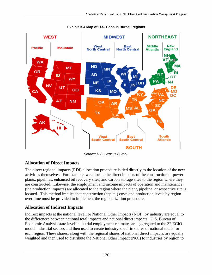
Analysis of Benefits of the NETL Clean Coal and Carbon Management Program
130
Exhibit B-4 Map of U.S. Census Bureau regions
Source: U.S. Census Bureau
Allocation of Direct Impacts
The direct regional impacts (RDI) allocation procedure is tied directly to the location of the new
activities themselves. For example, we allocate the direct impacts of the construction of power
plants, pipelines, enhanced oil recovery sites, and carbon storage sites to the region where they
are constructed. Likewise, the employment and income impacts of operation and maintenance
(the production impacts) are allocated to the region where the plant, pipeline, or respective site is
located. This method implies that construction (capital) costs and production levels by region
over time must be provided to implement the regionalization procedure.
Allocation of Indirect Impacts
Indirect impacts at the national level, or National Other Impacts (NOI), by industry are equal to
the differences between national total impacts and national direct impacts. U.S. Bureau of
Economic Analysis state level industrial employment estimates are aggregated to the 32 ECIO
model industrial sectors and then used to create industry-specific shares of national totals for
each region. These shares, along with the regional shares of national direct impacts, are equally
weighted and then used to distribute the National Other Impact (NOI) to industries by region to

Analysis of Benefits of the NETL Clean Coal and Carbon Management Program
131
compute Regional Other Impacts (ROI). The estimate of Regional Total Impact (RTI) is then
equal to ROI + RDI.
Implementation of Regionalization Mechanism
The flow chart in Exhibit B-5 provides an example of the linkages and sequence of steps
followed in estimating the regional impacts. Generally, the following steps summarize the
procedure:
ECIO model is run twice, once for a baseline and once for an impact (or economic
“shock”) scenario and the national total impacts (NTI) are computed.
National Direct Impact (NDI) is computed directly from the national baseline and impact
scenario data.
National Other (indirect and income induced) impact (NOI) is estimated as the difference
between NTI and NDI.
Regional Direct Impact (RDI) is derived from the regional baseline and impact scenario
data.
Regional Shares (RS) are computed as described above.
Using the regional shares, Regional Other Impact (ROI) is computed from NOI.
Regional Total Impact (RTI) is then the sum of RDI and ROI.
Exhibit B-5 Flow chart of regionalization mechanism

Analysis of Benefits of the NETL Clean Coal and Carbon Management Program
132
Appendix B.4: Model Outputs
The ECIO model generates forecasts for numerous economic variables, but focuses on
employment and income by industry and gross product. In its current version, the EViews®
process generates forecasts for all variables in the Appendix, but the additional utilities
developed for post-processing and report generation provide annual forecasts through 2040 for
these employment, income, and gross product by industry and in summary for the U.S. There
are two post-processing applications, one for national impacts and one for regional. The former
reads data from the two separate runs (base and shock scenarios) and computes impacts as
differences between the two forecasts. When region-specific direct impacts are provided, the
latter (regionalization) utility can be used to generate total impacts for employment, income, and
output by region. Details on specific output variables and files can be found in the accompanying
Operating Guide.

Analysis of Benefits of the NETL Clean Coal and Carbon Management Program
133
Appendix B.5: Equations and Variables of the Macroeconomic Econometric
Module
Stochastic Equations
Household Sector
1 log(CS/POP ) cnst2, cnst, AG1, AG2, AG3, log(CS/P OP )-1, log[Y D/(P OP · P H)], RSA, log(AA/P OP )−1
[Consumer expenditures: services]
2 log(CN/POP ) cnst2, cnst, AG1, AG2, AG3, log(CN/P OP )−1, ∆ log(CN/P OP )−1, log(AA/P OP )−1, log[Y D/(P OP · P H)], RMA
[Consumer expenditures: nondurables]
3 ∆CD/POP cnst2, cnst, AG1, AG2, AG3, DELD(KD/P OP )−1 − (CD/P OP )−1, (KD/P OP )−1, Y D/(P OP · P H), RMA · CDA, (AA/P OP )−1
[Consumer expenditures: durables]
4 ∆IHH/POP cnst2, cnst, DELH(KH/P OP )−1 − (IHH/P OP )−1, (KH/P OP )−1, (AA/P OP )−1, Y D/(P OP · P H), RMA−1IHHA, RHO = 2
[Residential investment–h]
5 log(L1/POP1) cnst, log(L1/P OP 1)−1, log(AA/P OP )−1, UR
[Labor force–men 25-54]
6 log(L2/POP2) cnst, log(L2/P OP 2)−1, log(W A/P H), log(AA/P OP )−1
[Labor force–women 25-54]
7 log(L3/POP3) cnst, log(L3/P OP 1)−1), log(W A/P H), log(AA/P OP )−1, UR
[Labor force–all others 16+]
8 log(LM/POP ) cnst, log(LM/P OP )−1, log(W A/P H), UR
[Number of moonlighters]

Analysis of Benefits of the NETL Clean Coal and Carbon Management Program
134
Firm Sector
9 log P F log P F−1, log[W F (1 + D5G)] − log LAM , cnst2, T B, cnst, T , log P IM , UR
[Price deflator for non farm sales]
10 log Y cnst, log Y−1, log X, log V−1, D593, D594, D601, RHO = 3
[Production–f]
11 ∆ log KK cnst2, cnst, log(KK/KKMIN )−1, ∆ log KK−1, ∆ log Y , ∆ log Y−1, ∆ log Y−2, ∆ log Y−3, ∆ log Y−4, ∆ log Y−5, RB−2(1 − D2G−2 − D2S−2) −100(P D−2/P D−6) − 1), (CG−2 + CG−3 + CG−4)/(P X−2Y S−2 + P X−3Y S−3 + P X−4Y S−4)
[Stock of capital–f]
12 ∆ log JF cnst, log[JF/(JHMIN/HF S)]−1, ∆ log JF−1, ∆ log Y , D593
[Number of jobs–f]
13 ∆ log HF cnst, log(HF/HF S)−1, log[JF/(JHMIN/HF S)]−1, ∆ log Y , T
[Average number of hours paid per job–f]
14 log HO cnst, HF F , HF F−1, RHO = 1
[Average number of overtime hours paid per job–f]
15 log W F − log LAM log W F−1 − log LAM−1, log P F , cnst, T , log P F−1
[Average hourly earnings excluding overtime–f]
16 log(MF/P F ) cnst, T , log(MF−1/P F ), log(X − F A), RS(1 − D2G − D2S)
[Demand deposits and currency–f]
17 ∆ log DF log[(P IEF − T F G − T F S − T F R)/DF−1]
[Dividends paid–f]
18 INT F/(−AF ) cnst, [INT F/(−AF )]−1, (1/400)[.4RS+.6(1/8)(RB+RB−1 +RB−2 +RB−3 + RB−4 + RB−5 + RB−6 + RB−7)], RHO = 1
[Interest payments–f]

Analysis of Benefits of the NETL Clean Coal and Carbon Management Program
135
Financial Sector
19 RB − RS−2 cnst, RB−1 − RS−2, RS − RS−2, RS−1 − RS−2, RHO = 1 [Bond rate]
20 RM − RS−2 cnst, RM−1 − RS−2, RS − RS−2, RS−1 − RS−2 [Mortgage rate] 21 CG/(P X−1 • Y S−1) cnst, ∆RB, [∆(P IEF − T F G − T F S − T F R)]/(P X−1 • Y S−1) [Capital gains or losses on the financial assets of h] 22 log[CUR/(P OP • P
F )] cnst, log[CUR−1/(P OP−1P F )], log[(X − F A)/P OP ], RSA, RHO = 1
[Currency held outside banks]
Import Equation
23 log(IM/P OP ) cnst2, cnst, log(IM/P OP )−1, log[(CS + CN + CD + IHH + IKF + IHB + IHF + IKB + IKH)/P OP ], log(P F/P IM ), D691, D692, D714, D721
[Imports]
Government Sectors
24 log UB cnst, log UB−1, log U , log W F , RHO = 1 [Unemployment insurance benefits] 25 INT G/(−AG) cnst, [INT G/(−AG)]−1, (1/400)[.4RS + .75(.6)(1/8)(RB + RB−1 + RB−2 +
RB−3 + RB−4 + RB−5 + RB−6 + RB−7)], RHO = 1 26 RS cnst, RS−1, 100[(P D/P D−1)4 −1], UR, ∆UR, P CM 1−1, D794823• P CM
1−1, ∆RS−1, ∆RS−2 [Three-month Treasury bill rate]
Identities
Exhibit B-6 Identities of the Macroeconomic Econometric model
Eq. LHS Variable
Explanatory Variables Description
27 P X = [P F (X − F A) + P F A · F A]/X [Price deflator for total sales]
28 P EX = P SI1 · P X [Price deflator for EX]
29 P D = (P X · X − P EX · EX + P IM · IM )/(X − EX + IM ) [Price deflator for domestic sales]
30 P H = (P CS · CS + P CN · CN + P CD · CD + P IH · IHH + IBT G + IBT S)/(CS + CN + CD + IHH)
[Price deflator for (CS + CN + CD + IHH) inclusive of indirect
business taxes]
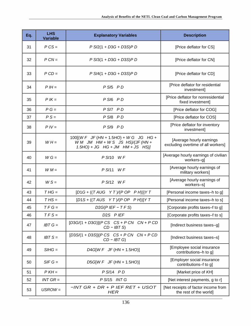
Analysis of Benefits of the NETL Clean Coal and Carbon Management Program
136
Eq. LHS Variable
Explanatory Variables Description
31 P CS = P SI2(1 + D3G + D3S)P D [Price deflator for CS]
32 P CN = P SI3(1 + D3G + D3S)P D [Price deflator for CN]
33 P CD = P SI4(1 + D3G + D3S)P D [Price deflator for CD]
34 P IH = P SI5 · P D [Price deflator for residential
investment]
35 P IK = P SI6 · P D [Price deflator for nonresidential
fixed investment]
36 P G = P SI7 · P D [Price deflator for COG]
37 P S = P SI8 · P D [Price deflator for COS]
38 P IV = P SI9 · P D [Price deflator for inventory
investment]
39 W H = 100[(W F · JF (HN + 1.5HO) + W G · JG · HG +
W M · JM · HM + W S · JS ·HS)/(JF (HN + 1.5HO) + JG · HG + JM · HM + JS · HS)]
[Average hourly earnings excluding overtime of all workers]
40 W G = P SI10 · W F [Average hourly earnings of civilian
workers–g]
41 W M = P SI11 · W F [Average hourly earnings of
military workers]
42 W S = P SI12 · W F [Average hourly earnings of
workers–s]
43 T HG = [D1G + ((T AUG · Y T )/(P OP · P H))]Y T [Personal income taxes–h to g]
44 T HS = [D1S + ((T AUS · Y T )/(P OP · P H))]Y T [Personal income taxes–h to s]
45 T F G = D2G(P IEF − T F S) [Corporate profits taxes–f to g]
46 T F S = D2S · P IEF [Corporate profits taxes–f to s]
47 IBT G = [D3G/(1 + D3G)](P CS · CS + P CN · CN + P CD
· CD − IBT S) [Indirect business taxes–g]
48 IBT S = [D3S/(1 + D3S)](P CS · CS + P CN · CN + P CD
· CD − IBT G) [Indirect business taxes–s]
49 SIHG = D4G[W F · JF (HN + 1.5HO)] [Employee social insurance
contributions–h to g]
50 SIF G = D5G[W F · JF (HN + 1.5HO)] [Employer social insurance
contributions–f to g]
51 P KH = P SI14 · P D [Market price of KH]
52 INT GR = P SI15 · INT G [Net interest payments, g to r]
53 USROW = −INT GR + DR + P IEF RET + USOT
HER [Net receipts of factor income from
the rest of the world]
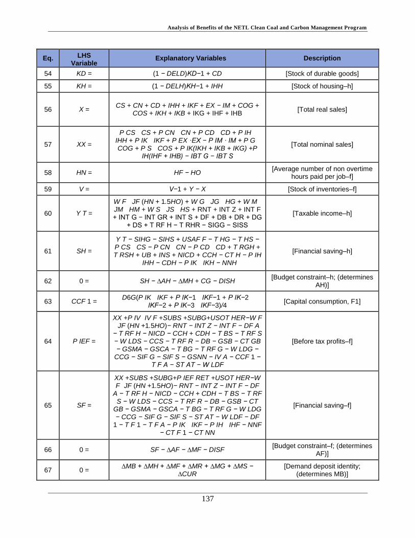
Analysis of Benefits of the NETL Clean Coal and Carbon Management Program
137
Eq. LHS Variable
Explanatory Variables Description
54 KD = (1 − DELD)KD−1 + CD [Stock of durable goods]
55 KH = (1 − DELH)KH−1 + IHH [Stock of housing–h]
56 X = CS + CN + CD + IHH + IKF + EX − IM + COG +
COS + IKH + IKB + IKG + IHF + IHB [Total real sales]
57 XX =
P CS · CS + P CN · CN + P CD · CD + P IH · IHH + P IK · IKF + P EX ·EX − P IM · IM + P G · COG + P S · COS + P IK(IKH + IKB + IKG) +P
IH(IHF + IHB) − IBT G − IBT S
[Total nominal sales]
58 HN = HF − HO [Average number of non overtime
hours paid per job–f]
59 V = V−1 + Y − X [Stock of inventories–f]
60 Y T =
W F · JF (HN + 1.5HO) + W G · JG · HG + W M · JM · HM + W S · JS · HS + RNT + INT Z + INT F + INT G − INT GR + INT S + DF + DB + DR + DG
+ DS + T RF H − T RHR − SIGG − SISS
[Taxable income–h]
61 SH =
Y T − SIHG − SIHS + USAF F − T HG − T HS − P CS · CS − P CN · CN − P CD · CD + T RGH + T RSH + UB + INS + NICD + CCH − CT H − P IH
· IHH − CDH − P IK · IKH − NNH
[Financial saving–h]
62 0 = SH − ∆AH − ∆MH + CG − DISH [Budget constraint–h; (determines
AH)]
63 CCF 1 = D6G(P IK · IKF + P IK−1 · IKF−1 + P IK−2 ·
IKF−2 + P IK−3 · IKF−3)/4 [Capital consumption, F1]
64 P IEF =
XX +P IV ·IV F +SUBS +SUBG+USOT HER−W F ·JF (HN +1.5HO)− RNT − INT Z − INT F − DF A
− T RF H − NICD − CCH + CDH − T BS − T RF S − W LDS − CCS − T RF R − DB − GSB − CT GB − GSMA − GSCA − T BG − T RF G − W LDG −
CCG − SIF G − SIF S − GSNN − IV A − CCF 1 − T F A − ST AT − W LDF
[Before tax profits–f]
65 SF =
XX +SUBS +SUBG+P IEF RET +USOT HER−W F ·JF (HN +1.5HO)− RNT − INT Z − INT F − DF
A − T RF H − NICD − CCH + CDH − T BS − T RF S − W LDS − CCS − T RF R − DB − GSB − CT
GB − GSMA − GSCA − T BG − T RF G − W LDG − CCG − SIF G − SIF S − ST AT − W LDF − DF
1 − T F 1 − T F A − P IK · IKF − P IH · IHF − NNF − CT F 1 − CT NN
[Financial saving–f]
66 0 = SF − ∆AF − ∆MF − DISF [Budget constraint–f; (determines
AF)]
67 0 = ∆MB + ∆MH + ∆MF + ∆MR + ∆MG + ∆MS −
∆CUR [Demand deposit identity;
(determines MB)]

Analysis of Benefits of the NETL Clean Coal and Carbon Management Program
138
Eq. LHS Variable
Explanatory Variables Description
68 SB = GSB − CT B − P IH · IHB − P IK · IKB [Financial saving–b]
69 0 = SB − ∆AB − ∆MB − ∆(BR − BO) − DISB [Budget constraint–b; (determines
AB)]
70 SR = −P EX · EX − USROW + P IM · IM + T F R + T RF R + T RHR + T RGR − USAF F −
CT R − NNR [Financial saving–r]
71 0 = SR − ∆AR − ∆MR + ∆Q − DISR [Budget constraint–r; (determines
AR)]
72 SG =
GSMA + GSCA + T HG + IBT G + T BG + T F G + SIHG + SIF G − DG + T RF G − P G · COG − W G · JG · HG − W M · JM · HM − T RGH − T
RGR − T RGS − INT G − SUBG + W LDG + CCG − INS − USAF F − CT GMB − NNG − P IK · IKG
+ SIGG
[Financial saving–g]
73 0 = SG − ∆AG − ∆MG + ∆CUR + ∆(BR − BO) − ∆Q −
DISG [Budget constraint–g; (determines
AG unless AG is exogenous)]
74 SS =
T HS + IBT S + T BS + T F S + SIHS + SIF S − DS + T RGS + T RF S −P S · COS − W S · JS ·
HS − T RSH − UB − INT S − SUBS + W LDS +CCS − CT S − NNS + SISS
[Financial saving–s]
75 0 = SS − ∆AS − ∆MS − DISS [Budget constraint–s; (determines
AS)]
76 0 = SH + SF + SB + SR + SG + SS + ST AT + W LDF + USAF F
[Redundant equation—for checking]
77 M 1 = M 1−1 + ∆MH + ∆MF + ∆MR + ∆MS + MDIF [Money supply]
78 GDP = XX + P IV (V − V−1) + IBT G + IBT S + W G · JG
· HG + W M · JM · HM + W S · JS · HS [Nominal GDP]
79 GDP R = Y + P SI13(JG · HG + JM · HM + JS · HS) + ST
AT P [Real GDP]
80 GDP D = GDP/GDP R [GDP price deflator]
81 E = JF + JG + JM + JS − LM [Total employment, civilian and
military]
82 U = L1 + L2 + L3 − E [Number of people unemployed]
83 UR = U/(L1 + L2 + L3 − JM ) [Civilian unemployment rate]
84 DF 1 = DF − DF A [Net dividends paid, F1]
85 AA = (AH + MH)/P H + (P KH · KH)/P H [Total net wealth–h]
86 D1GM = D1G + (2T AUG · Y T )/(P OP · P H) [Marginal personal income tax
rate–g]
87 D1SM = D1S + (2T AUS · Y T )/(P OP · P H) [Marginal personal income tax
rate–s]
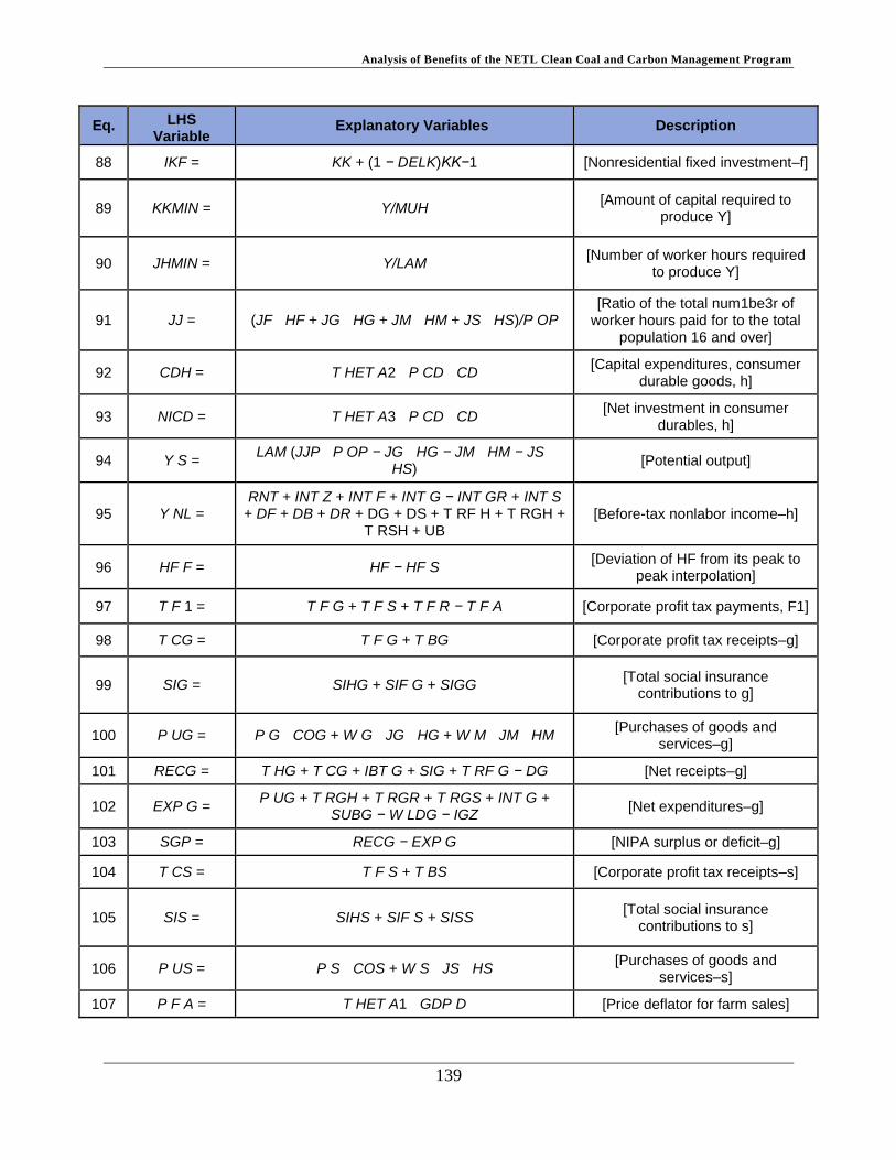
Analysis of Benefits of the NETL Clean Coal and Carbon Management Program
139
Eq. LHS Variable
Explanatory Variables Description
88 IKF = KK + (1 − DELK)KK−1 [Nonresidential fixed investment–f]
89 KKMIN = Y/MUH [Amount of capital required to
produce Y]
90 JHMIN = Y/LAM [Number of worker hours required
to produce Y]
91 JJ = (JF · HF + JG · HG + JM · HM + JS · HS)/P OP [Ratio of the total num1be3r of
worker hours paid for to the total population 16 and over]
92 CDH = T HET A2 · P CD · CD [Capital expenditures, consumer
durable goods, h]
93 NICD = T HET A3 · P CD · CD [Net investment in consumer
durables, h]
94 Y S = LAM (JJP · P OP − JG · HG − JM · HM − JS ·
HS) [Potential output]
95 Y NL = RNT + INT Z + INT F + INT G − INT GR + INT S
+ DF + DB + DR + DG + DS + T RF H + T RGH + T RSH + UB
[Before-tax nonlabor income–h]
96 HF F = HF − HF S [Deviation of HF from its peak to
peak interpolation]
97 T F 1 = T F G + T F S + T F R − T F A [Corporate profit tax payments, F1]
98 T CG = T F G + T BG [Corporate profit tax receipts–g]
99 SIG = SIHG + SIF G + SIGG [Total social insurance
contributions to g]
100 P UG = P G · COG + W G · JG · HG + W M · JM · HM [Purchases of goods and
services–g]
101 RECG = T HG + T CG + IBT G + SIG + T RF G − DG [Net receipts–g]
102 EXP G = P UG + T RGH + T RGR + T RGS + INT G +
SUBG − W LDG − IGZ [Net expenditures–g]
103 SGP = RECG − EXP G [NIPA surplus or deficit–g]
104 T CS = T F S + T BS [Corporate profit tax receipts–s]
105 SIS = SIHS + SIF S + SISS [Total social insurance
contributions to s]
106 P US = P S · COS + W S · JS · HS [Purchases of goods and
services–s]
107 P F A = T HET A1 · GDP D [Price deflator for farm sales]

Analysis of Benefits of the NETL Clean Coal and Carbon Management Program
140
Eq. LHS Variable
Explanatory Variables Description
108 RECS = T HS + T CS + IBT S + SIS + T RGS + T RF S −
DS [Net receipts–s]
109 EXP S = P US + T RSH + UB + INT S + SUBS − W LDS −
ISZ [Net expenditures–s]
110 SSP = RECS − EXP S [NIPA surplus or deficit–s]
111 Y D =
W F · JF (HN + 1.5HO) + W G · JG · HG + W M · JM · HM + W S · JS · HS + RNT + INT Z + INT F + INT G − INT GR + INT S + DF + DB + DR + DG + DS + T RF H + T RGH + T RSH + UB − SIHG − SIHS + USAF F − T HG − T HS − T RHR − SIGG
− SISS
[Disposable income–h]
112 SRZ = (Y D − P CS · CS − P CN · CN − P CD · CD)/Y D [Approximate NIPA saving rate–h]
113 IV F = V − V−1 [Inventory investment–f]
114 P ROD = Y/(JF · HF ) [Output per paid for worker hour:
“productivity"]
115 W R = W F/P F [Real wage rate of workers in f]
116 P OP = P OP 1 + P OP 2 + P OP 3 [Noninstitutional population 16 and
over]
117 SHRP IE = [(1 − D2G − D2S)P IEF ]/[W F · JF (HN + 1.5HO)] [Ratio of after tax profits to the wage bill net of employer social
security taxes]
118 P CGDP R = 100[(GDP R/GDP R−1)4 − 1] [Percentage change in GDPR]
119 P CGDP D = 100[(GDP D/GDP D−1)4 − 1] [Percentage change in GDPD]
120 P CM 1 = 100[(M 1/M 1−1)4 − 1] [Percentage change in M1]
121 UBR = BR − BO [Unborrowed reserves]
122 W A =
100[(1 − D1GM − D1SM − D4G)[W F · JF (HN + 1.5HO)] + (1 − D1GM − D1SM )(W G · JG · HG +
W M · JM · HM + W S · JS · HS − SIGG − SISS)]/[JF (HN + 1.5HO) + JG · HG + JM · HM +
JS · HS]
[After tax wage rate]
123 RSA = RS(1 − D1GM − D1SM ) [After-tax three-month Treasury bill
rate]
124 RMA = RM (1 − D1GM − D1SM ) [After-tax mortgage rate]
125 GNP = GDP + USROW [Nominal GNP]
126 GNP R = GDP R + USROW/GDP D [Real GNP]
127 GNP D = GNP/GNP R [GNP price deflator]
128 P IEF RET = T HET A4 · P IEF [Foreign earnings retained
abroad—f]
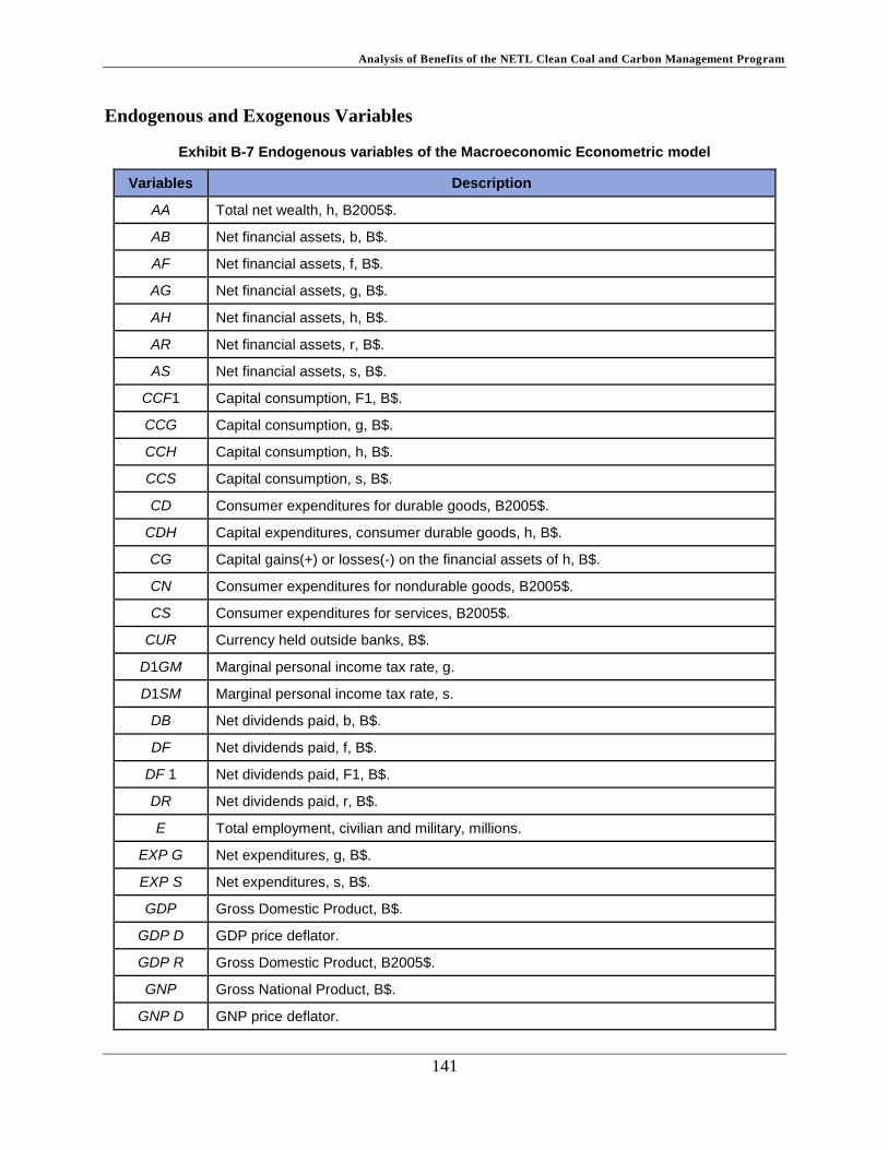
Analysis of Benefits of the NETL Clean Coal and Carbon Management Program
141
Endogenous and Exogenous Variables
Exhibit B-7 Endogenous variables of the Macroeconomic Econometric model
Variables Description
AA Total net wealth, h, B2005$.
AB Net financial assets, b, B$.
AF Net financial assets, f, B$.
AG Net financial assets, g, B$.
AH Net financial assets, h, B$.
AR Net financial assets, r, B$.
AS Net financial assets, s, B$.
CCF1 Capital consumption, F1, B$.
CCG Capital consumption, g, B$.
CCH Capital consumption, h, B$.
CCS Capital consumption, s, B$.
CD Consumer expenditures for durable goods, B2005$.
CDH Capital expenditures, consumer durable goods, h, B$.
CG Capital gains(+) or losses(-) on the financial assets of h, B$.
CN Consumer expenditures for nondurable goods, B2005$.
CS Consumer expenditures for services, B2005$.
CUR Currency held outside banks, B$.
D1GM Marginal personal income tax rate, g.
D1SM Marginal personal income tax rate, s.
DB Net dividends paid, b, B$.
DF Net dividends paid, f, B$.
DF 1 Net dividends paid, F1, B$.
DR Net dividends paid, r, B$.
E Total employment, civilian and military, millions.
EXP G Net expenditures, g, B$.
EXP S Net expenditures, s, B$.
GDP Gross Domestic Product, B$.
GDP D GDP price deflator.
GDP R Gross Domestic Product, B2005$.
GNP Gross National Product, B$.
GNP D GNP price deflator.

Analysis of Benefits of the NETL Clean Coal and Carbon Management Program
142
Variables Description
GNP R Gross National Product, B2005$.
GSB Gross saving, B, B$.
GSNN Gross saving, NN, B$.
HF Average number of hours paid per job, f, hours per quarter.
HF F Deviation of HF from its peak to peak interpolation.
HN Average number of non overtime hours paid per job, f, hours per quarter.
HO Average number of overtime hours paid per job, f, hours per quarter.
IBT G Indirect business taxes, g, B$.
IBT S Indirect business taxes, s, B$.
IGZ Gross investment, g, B$.
IHH Residential investment, h, B2005$.
IKF Nonresidential fixed investment, f, B2005$.
IM Imports, B2005$.
INT F Net interest payments, f, B$.
INT G Net interest payments, g, B$.
INT GR Net interest payments, g to r, B$.
INT Z Net interest payments, other, B$.
ISZ Gross investment, s, B$.
IV F Inventory investment, f, B2005$.
JF Number of jobs, f, millions.
JHMIN Number of worker hours required to produce Y, millions.
JJ Ratio of the total number of worker hours paid for to the total population 16 and over.
KD Stock of durable goods, B2005$.
KH Stock of housing, h, B2005$.
KK Stock of capital, f, B2005$.
KKMIN Amount of capital required to produce Y, B2005$.
L1 Labor force of men 25-54, millions.
L2 Labor force of women 25-54, millions.
L3 Labor force of all others, 16+, millions.
LM Number of “moonlighters": difference between the total number of jobs (establishment data) and the total number of people employed (household survey data), millions.
M 1 Money supply, end of quarter, B$.
MB Net demand deposits and currency, b, B$.

Analysis of Benefits of the NETL Clean Coal and Carbon Management Program
143
Variables Description
MF Demand deposits and currency, f, B$.
MG Demand deposits and currency, g, B$.
MH Demand deposits and currency, h, B$.
MR Demand deposits and currency, r, B$.
MS Demand deposits and currency, s, B$.
NICD Net investment in consumer durables, h, B$.
P CD Price deflator for CD.
P CGDP D Percentage change in GDPD, annual rate, percentage points.
P CGDP R Percentage change in GDPR, annual rate, percentage points.
P CM 1 Percentage change in M1, annual rate, percentage points.
P CN Price deflator for CN.
P CS Price deflator for CS.
P D Price deflator for X - EX + IM (domestic sales).
P EX Price deflator for EX.
P F Price deflator for non farm sales.
P F A Price deflator for farm sales.
P G Price deflator for COG.
P H Price deflator for CS + CN + CD + IHH inclusive of indirect busi-
P IEF Before tax profits, f, B$.
P IEF RET Foreign earnings retained abroad, f, B$.
P IH Price deflator for residential investment.
P IK Price deflator for nonresidential fixed investment.
P IV Price deflator for inventory investment, adjusted.
P KH Market price of KH.
P OP Noninstitutional population 16+, millions.
P ROD Output per paid for worker hour ("productivity").
P S Price deflator for COS.
P UG Purchases of goods and services, g, B$.
P US Purchases of goods and services, s, B$.
P X Price deflator for total sales.
Q Gold and foreign exchange, g, B$.
RB Bond rate, percentage points.
RECG Net receipts, g, B$.

Analysis of Benefits of the NETL Clean Coal and Carbon Management Program
144
Variables Description
RECS Net receipts, s, B$.
RM Mortgage rate, percentage points.
RMA After tax mortgage rate, percentage points.
RNT Rental income, h, B$.
RS Three-month Treasury bill rate, percentage points.
RSA After tax bill rate, percentage points.
SB Financial saving, b, B$.
SF Financial saving, f, B$.
SG Financial saving, g, B$.
SGP NIPA surplus (+) or deficit (-), g, B$.
SH Saving, h, B$.
SHRP IE Ratio of after tax profits to the wage bill net of employer social security taxes.
SIF G Employer social insurance contributions, f to g, B$.
SIG Total employer and employee social insurance contributions to g, B$.
SIHG Employee social insurance contributions, h to g, B$.
SIS Total employer and employee social insurance contributions to s, B$.
SR Financial saving, r, B$.
SRZ Approximate NIPA saving rate, h.
SS Financial saving, s, B$.
SSP NIPA surplus (+) or deficit (-), s, B$.
T BG Corporate profit taxes, b to g, B$.
T CG Corporate profit tax receipts, g, B$.
T CS Corporate profit tax receipts, s, B$.
T F 1 Corporate profit tax payments, F1, B$.
T F G Corporate profit taxes, f to g, B$.
T F S Corporate profit taxes, f to s, B$.
T HG Personal income taxes, h to g, B$.
T HS Personal income taxes, h to s, B$.
T RGH Transfer payments (net), g to h, B$.
T RGS Transfer payments, g to s, B$.
T RSH Transfer payments, s to h, excluding unemployment insurance benefits, B$.
U Number of people unemployed, millions.
UB Unemployment insurance benefits, B$.

Analysis of Benefits of the NETL Clean Coal and Carbon Management Program
145
Variables Description
UBR Unborrowed reserves, B$.
UR Civilian unemployment rate.
USROW Net receipts of factor income from the rest of the world, B$.
V Stock of inventories, f, B2005$.
W A After tax wage rate. (Includes supplements to wages and salaries except employer contributions for social insurance.)
W F Average hourly earnings excluding overtime of workers in f. (Includes supplements to wages and salaries except employer contributions for social insurance.)
W G Average hourly earnings of civilian workers in g. (Includes supplements to wages and salaries including employer contributions for social insurance.)
W H Average hourly earnings excluding overtime of all workers. (Includes supplements to wages and salaries except employer contributions for social insurance.)
W M Average hourly earnings of military workers. (Includes supplements to wages and salaries including employer contributions for social insurance.)
W R Real wage rate of workers in f. (Includes supplements to wages and salaries except employer contributions for social insurance.)
W S Average hourly earnings of workers in s. (Includes supplements to wages and salaries including employer contributions for social insurance.)
X Total sales, B2005$.
XX Total sales, B$.
Y Total production, B2005$.
Y D Disposable income, h, B$.
Y NL Before tax nonlabor income, h, B$.
Y S Potential output, B2005$.
Y T Taxable income, h, B$.
Exhibit B-8 Exogenous variables of the Macroeconomic Econometric model
Variables Description
AG1 Percent of 16+ population 26-55 minus percent 16-25.
AG2 Percent of 16+ population 56-65 minus percent 16-25.
AG3 Percent of 16+ population 66+ minus percent 16-25.
BO Bank borrowing from the Fed, B$.

Analysis of Benefits of the NETL Clean Coal and Carbon Management Program
146
Variables Description
BR Total bank reserves, B$.
CCGQ Capital consumption, g, B2005$.
CCHQ Capital consumption, h, B2005$.
CCSQ Capital consumption, s, B2005$.
CDA Peak to peak interpolation of CD/POP.
COG Purchases of consumption and investment goods, g, B2005$.
COS Purchases of consumption and investment goods, s, B2005$.
CT B Net capital transfers paid, financial corporations, B$.
CT F 1 Net capital transfers paid, nonfinancial corporations, B$.
CT GB Financial stabilization payments, B$.
CT GMB Net capital transfers paid, g, less financial stabilization payments,B$.
CT H Net capital transfers paid, h, B$.
CT NN Net capital transfers paid, noncorporate business, B$.
CT R Net capital transfers paid, r, B$.
CT S Net capital transfers paid, s, B$.
D1G Personal income tax parameter, g.
D1S Personal income tax parameter, s.
D2G Profit tax rate, g.
D2S Profit tax rate, s.
D3G Indirect business tax rate, g.
D3S Indirect business tax rate, s.
D4G Employee social security tax rate, g.
D593 1 in 1959:3; 0 otherwise.
D594 1 in 1959:4; 0 otherwise.
D5G Employer social security tax rate, g.
D601 1 in 1960:1; 0 otherwise.
D691 1 in 1969:1; 0 otherwise.
D692 1 in 1969:2; 0 otherwise. 3
D6G Capital consumption rate for CCF1, g.
D714 1 in 1971:4; 0 otherwise.
D721 1 in 1972:1; 0 otherwise.
D794823 1 in 1979:4-1982:3; 0 otherwise.
DBQ Net dividends paid, b, B2005$.
DELD Physical depreciation rate of the stock of durable goods, rate per quarter.
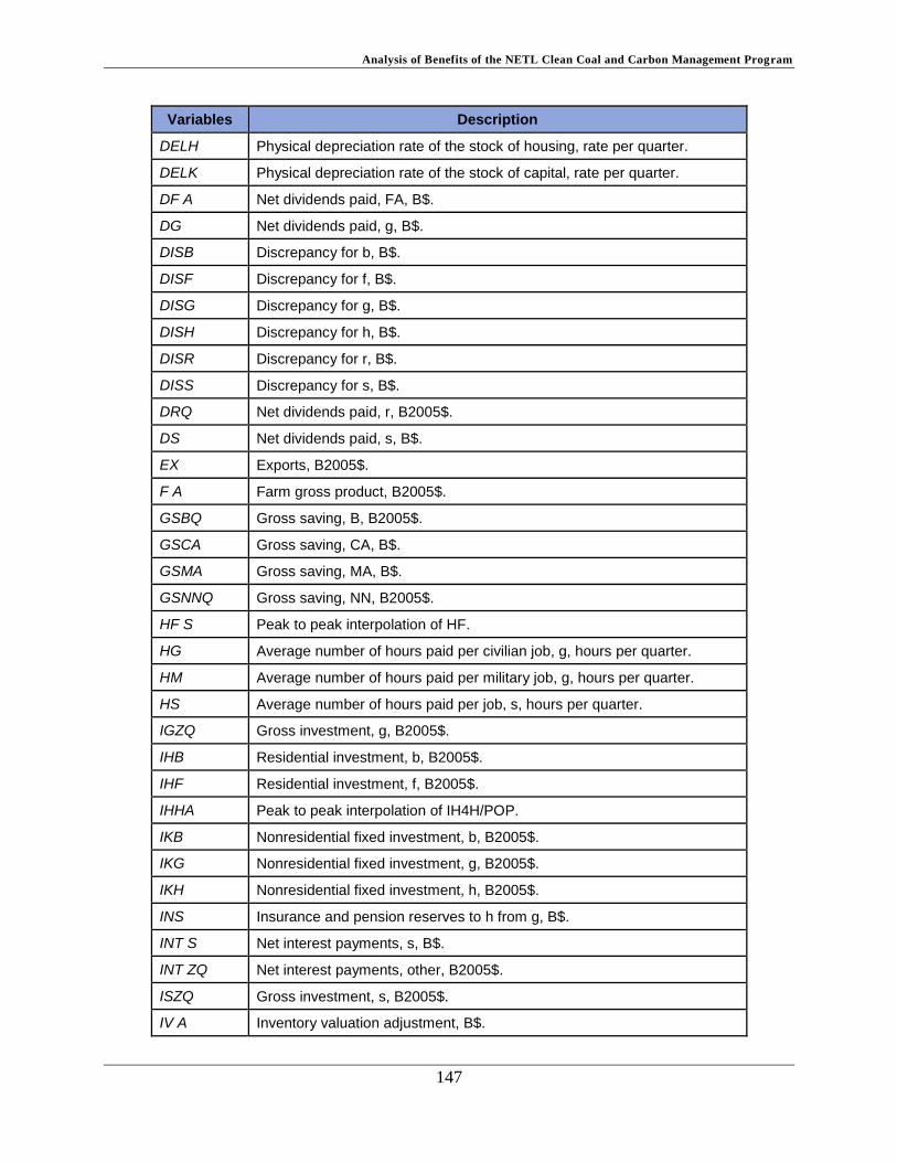
Analysis of Benefits of the NETL Clean Coal and Carbon Management Program
147
Variables Description
DELH Physical depreciation rate of the stock of housing, rate per quarter.
DELK Physical depreciation rate of the stock of capital, rate per quarter.
DF A Net dividends paid, FA, B$.
DG Net dividends paid, g, B$.
DISB Discrepancy for b, B$.
DISF Discrepancy for f, B$.
DISG Discrepancy for g, B$.
DISH Discrepancy for h, B$.
DISR Discrepancy for r, B$.
DISS Discrepancy for s, B$.
DRQ Net dividends paid, r, B2005$.
DS Net dividends paid, s, B$.
EX Exports, B2005$.
F A Farm gross product, B2005$.
GSBQ Gross saving, B, B2005$.
GSCA Gross saving, CA, B$.
GSMA Gross saving, MA, B$.
GSNNQ Gross saving, NN, B2005$.
HF S Peak to peak interpolation of HF.
HG Average number of hours paid per civilian job, g, hours per quarter.
HM Average number of hours paid per military job, g, hours per quarter.
HS Average number of hours paid per job, s, hours per quarter.
IGZQ Gross investment, g, B2005$.
IHB Residential investment, b, B2005$.
IHF Residential investment, f, B2005$.
IHHA Peak to peak interpolation of IH4H/POP.
IKB Nonresidential fixed investment, b, B2005$.
IKG Nonresidential fixed investment, g, B2005$.
IKH Nonresidential fixed investment, h, B2005$.
INS Insurance and pension reserves to h from g, B$.
INT S Net interest payments, s, B$.
INT ZQ Net interest payments, other, B2005$.
ISZQ Gross investment, s, B2005$.
IV A Inventory valuation adjustment, B$.

Analysis of Benefits of the NETL Clean Coal and Carbon Management Program
148
Variables Description
JG Number of civilian jobs, g, millions.
JJP Potential value of JJ.
JM Number of military jobs, g, millions.
JS Number of jobs, s, millions.
LAM Amount of output capable of being produced per worker hour.
MDIF
Net increase in demand deposits and currency of banks in U.S. possessions plus change in demand deposits and currency of private nonbank financial institutions plus change in demand deposits and currency of federally sponsored credit agencies and mortgage pools minus mail float, U.S. government, B$.
MGQ Demand deposits and currency, g, B2005$.
MHQ Demand deposits and currency, h, B2005$.
MRQ Demand deposits and currency, r, B2005$.
MSQ Demand deposits and currency, s, B2005$.
MUH Amount of output capable of being produced per unit of capital.
NNF Net acquisition of nonproduced nonfinancial assets, f, B$.
NNG Net acquisition of nonproduced nonfinancial assets, g, B$.
NNH Net acquisition of nonproduced nonfinancial assets, h, B$.
NNR Net acquisition of nonproduced nonfinancial assets, r, B$.
NNS Net acquisition of nonproduced nonfinancial assets, s, B$.
P IM Price deflator for IM.
P OP 1 Noninstitutional population of men 25-54, millions.
P OP 2 Noninstitutional population of women 25-54, millions.
P OP 3 Noninstitutional population of all others, 16+, millions.
P SI1 Ratio of PEX to PX.
P SI10 Ratio of WG to WF.
P SI11 Ratio of WM to WF.
P SI12 Ratio of WS to WF.
P SI13 Ratio of gross product of g and s to total employee hours of g and s.
P SI14 Ratio of PKH to PD.
P SI15 Ratio of INTGR to INTG.
P SI2 Ratio of PCS to (1 + D3G + D3S)PD.
P SI3 Ratio of PCN to (1 + D3G + D3S)PD.
P SI4 Ratio of PCD to (1 + D3G + D3S)PD.
P SI5 Ratio of PIH to PD.
P SI6 Ratio of PIK to PD.

Analysis of Benefits of the NETL Clean Coal and Carbon Management Program
149
Variables Description
P SI7 Ratio of PG to PD.
P SI8 Ratio of PS to PD.
P SI9 Ratio of PIV to PD.
QQ Gold and foreign exchange, g6, B2005$.
RNT Q Rental income, h, B2005$.
SIF S Employer social insurance contributions, f to s, B$.
SIGG Employer social insurance contributions, g to g, B$.
SIHS Employee social insurance contributions, h to s, B$.
SISS Employer social insurance contributions, s to s, B$.
ST AT Statistical discrepancy, B$.
ST AT P Statistical discrepancy relating to the use of chain type price indices, B2005$.
SUBG Subsidies less current surplus of government enterprises, g, B$.
SUBS Subsidies less current surplus of government enterprises, s, B$.
T 1 in 1952:1, 2 in 1952:2, etc.
T AUG Progressivity tax parameter in personal income tax equation for g.
T AUS Progressivity tax parameter in personal income tax equation for s.
T BGQ Corporate profit taxes, b to g, B2005$.
T BS Corporate profit taxes, b to s, B$.
T F A Corporate profit tax payments, FA, B$.
T F R Taxes, f to r, B$.
T HET A1 Ratio of P F A to GDP D.
T HET A2 Ratio of CDH to P CD · CD.
T HET A3 Ratio of NICD to P CD · CD.
T HET A4 Ratio of P IEF RET to P IEF.
T RF G Transfer payments, f to g, B$.
T RF H Transfer payments, f to h, B$.
T RF R Transfer payments, f to r, B$.
T RF S Transfer payments, f to s, B$.
T RGHQ Transfer payments (net), g to h, B2005$.
T RGR Transfer payments (net), g to r, B$.
T RGSQ Transfer payments, g to s, B2005$.
B$ = Billions of dollars.
B2005$ = Billions of 2005 dollars.

Analysis of Benefits of the NETL Clean Coal and Carbon Management Program
150
Appendix B.6: References
Conway Jr AR, R. S. (1990). The Washington projection and simulation model: a regional
interindustry econometric model. International Regional Science Review, 13(1-2):141.
Fair, Ray. Estimating How the Macroeconomy Works, Harvard University Press, 2004
www.netl.doe.gov
Pittsburgh, PA • Morgantown, WV • Albany, OR • Sugar Land, TX • Anchorage, AK
(800) 553-7681
Charles Zelek
David Erne