Embed Size (px)
Citation preview
Appendix A- Manufacturer Given Information and Rotor Drawings
Appendix A Manufacturer Given Information and Rotor Drawings
The first part of this section includes some given information from manufacturers, mainly
for meters A, B and C. The second part collates each rotor drawing that was produced by
Solidworks.
A. 1 Manufacturer Given Information
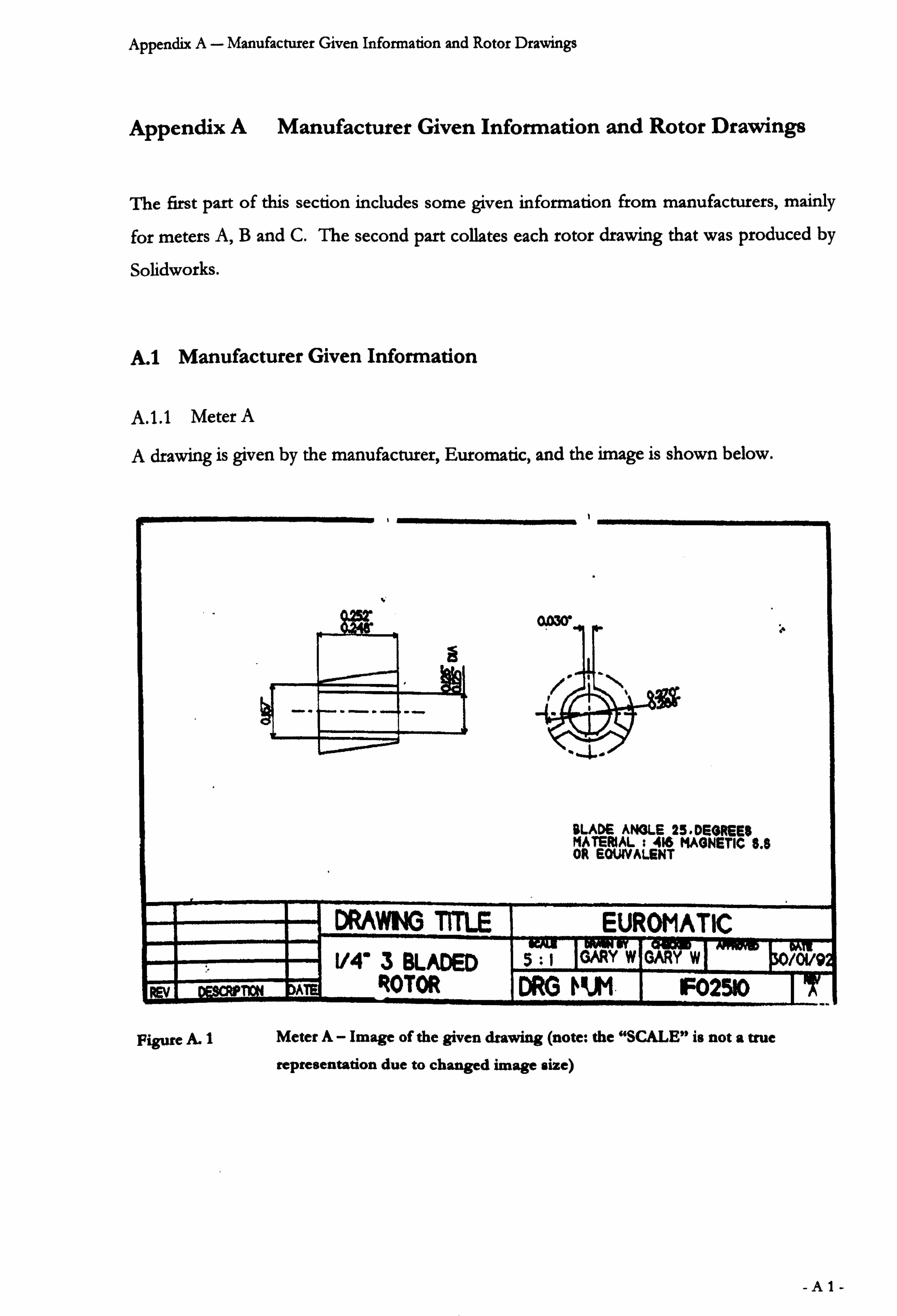
A. 1.1 Meter A
A drawing is given by the manufacturer, Euromatic, and the image is shown below.
BLADE ANGLE 25. DEOREES MATERIAL : 416 MAGNETIC 8.8 OR EQUIVALENT
DRAWNG TITLE EUROMATIC or, " ý IPT oil= V4'3 BLADED s= i cMY W GARY w /0v9
ROTOR DRG tRA F02510
Figure A. 1 Meter A- Image of the given drawing (note: the "SCALE" is not a true
representation due to changed image size)
-Al-
Appendix A- Manufacturer Given Information and Rotor Drawings
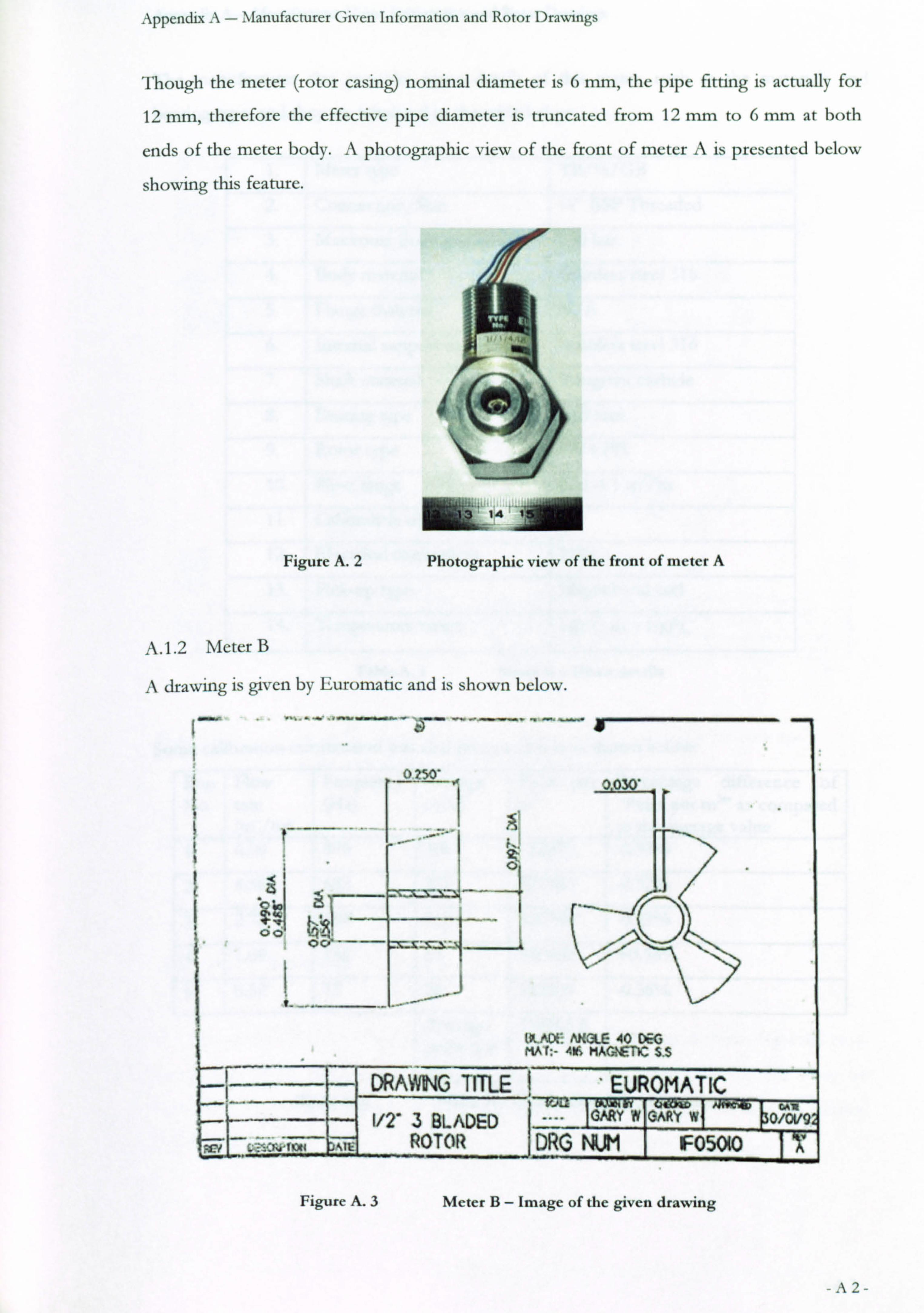
Though the meter (rotor casing) nominal diameter is 6 mm, the pipe fitting is actually for
12 mm, therefore the effective pipe diameter is truncated from 12 mm to 6 mm at both
ends of the meter body. A photographic view of the front of meter A is presented below
showing this feature.
Figure A. 2 Photographic view of the front of meter A
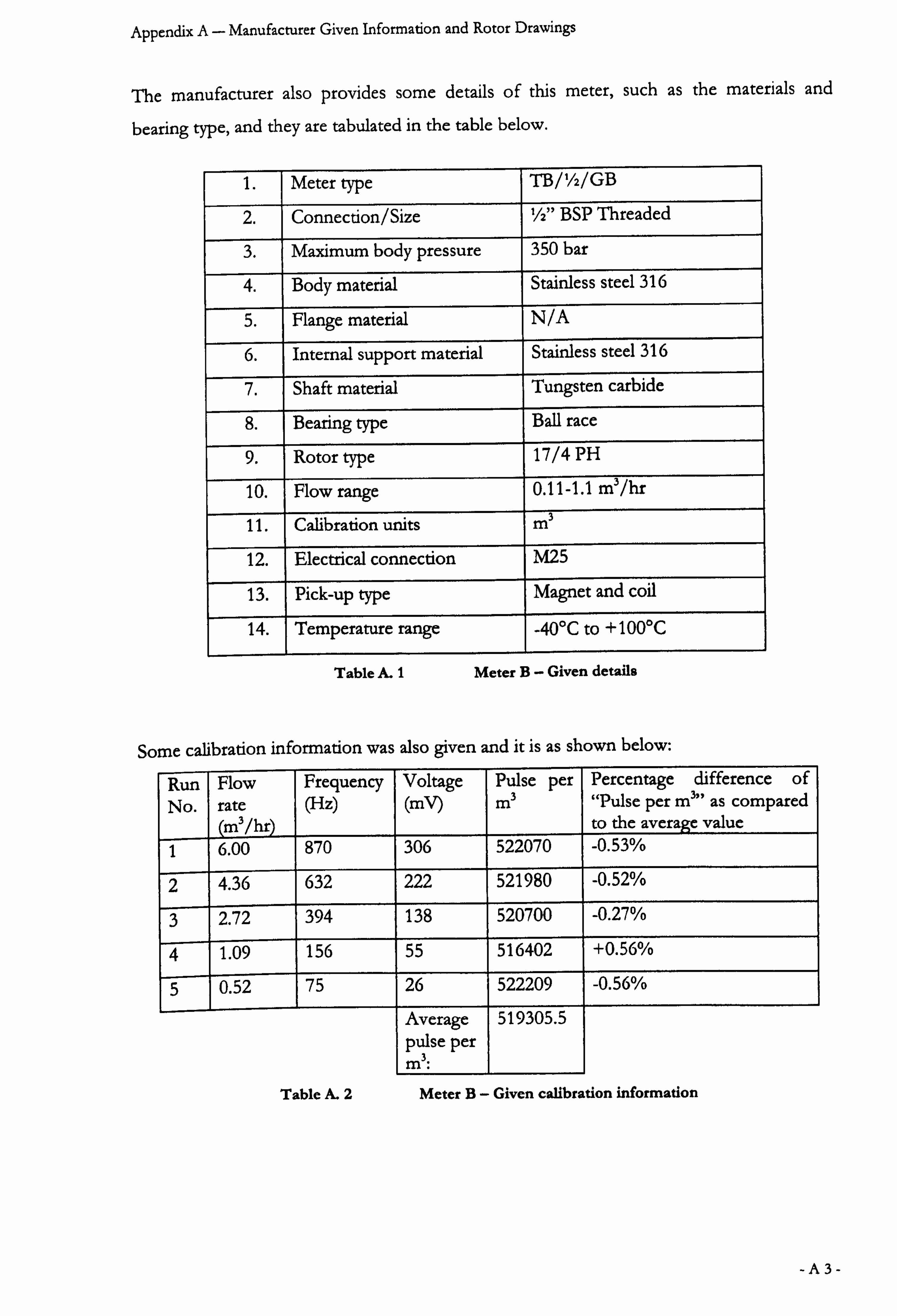
A. 1.2 Meter B
A drawing is given by Euromatic and is shown below.
p
ýý
ö0
(LAc* MOLE 40 DEG MAT: - 416 MAG, ¬T)C S. S
4E DRAWt G TITLE EUROMATIC I/2' 3 BLADED N CARY W oiöv9
ROTOR DRG NUM F050(0
Figure A. 3 Meter B- Image of the given drawing
-A2-
Appendix A- Manufacturer Given Information and Rotor Drawings
The manufacturer also provides some details of this meter, such as the materials and
bearing type, and they are tabulated in the table below.
1. Meter type TB/'/2/GB
2. Connection/Size '/x" BSP Threaded
3. Maximum body pressure 350 bar
4. Body material Stainless steel 316
5. Flange material N/A
6. Internal support material Stainless steel 316
7. Shaft material Tungsten carbide
8. Bearing type Ball race
9. Rotor type 17/4 PH
10. Flow range 0.11-1.1 m3/hr
11. Calibration units m3
12. Electrical connection M25
13. Pick-up type Magnet and coil
14. Temperature range -40°C to +100°C
Table A. 1 Meter B- Given details
Some calibration information was also given and it is as shown below:
Run No.
Flow rate (M3/hr)
Frequency (Hz)
Voltage (mV)
Pulse per m3
Percentage difference of "Pulse per m3" as compared to the average value
1 6.00 870 306 522070 -0.53%
2 4.36 632 222 521980 -0.52%
3 2.72 394 138 520700 -0.27%
4 1.09 156 55 516402 +0.56%
5 0.52 75 26 522209 -0.56% Average 519305.5 pulse per m3:
Table A. 2 Meter B- Given calibration information
-A3-
Appendix A- Manufacturer Given Information and Rotor Drawings
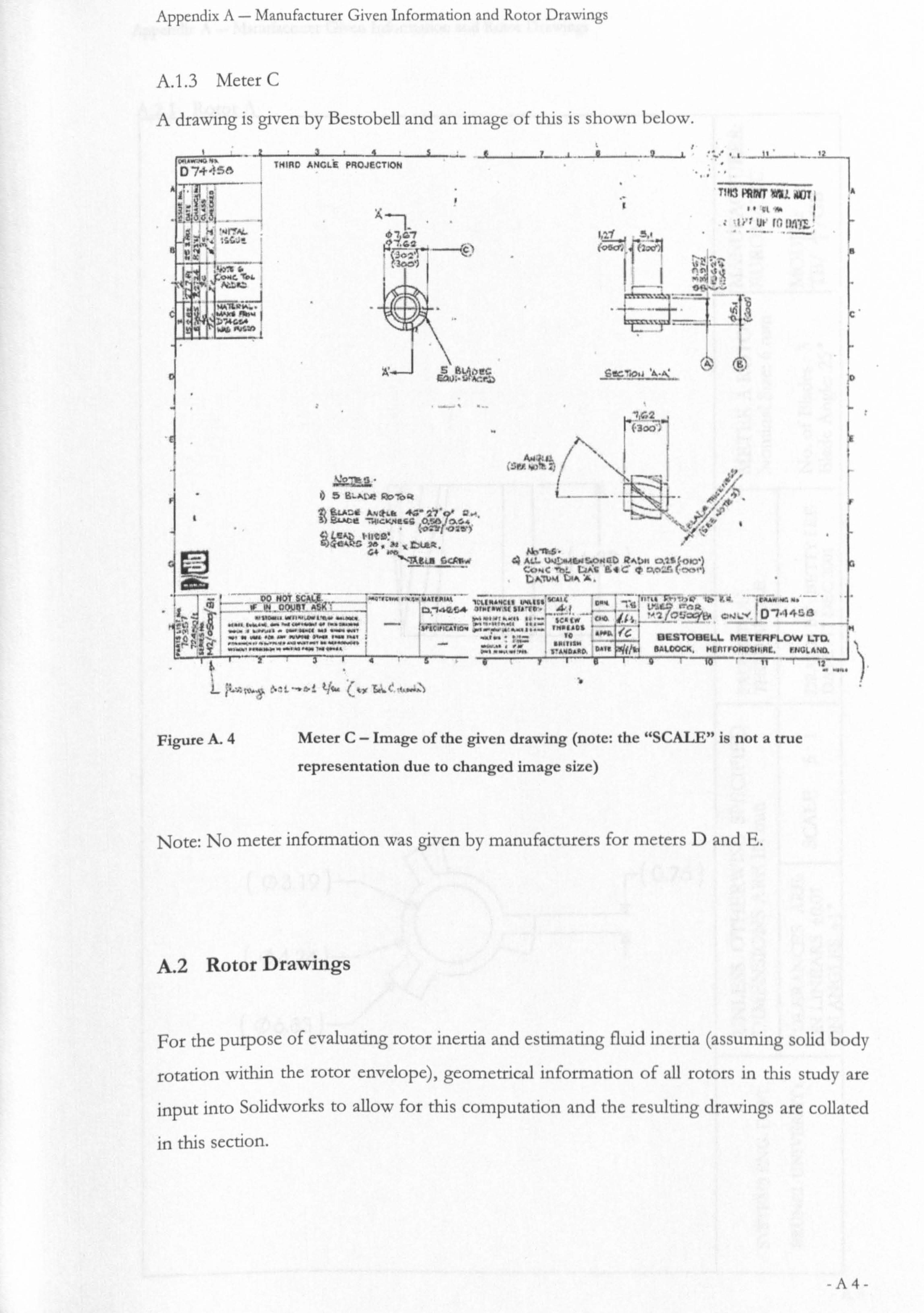
A. 1.3 Meter C
A drawing is given by Bestobell and an image of this is shown below.
L34Sw _0
4L +
..
. Iý 4 . _. 1L-_12
SA TMIRO ANGLE PROJECTION
lF ýclr 1
i%t Ur FG mir,
14 -- 3n2'
Oda
i
R4eeRý1 ý: ".
s Bý, poeG ýy 6
ý 6C1U: "Sý'Mý. y
SDCTiON 4"ý ,D
, 62
eN 7
M
aim-
EA4 AMt. a "Aßß 1.7" a-.
" F"O: i OIY) ýý °ý
ICEA,, "its.
771) 6CAVIW Q ALL W! A~ sQ0 ßw; >h qtt qp GA. T1+M GM A.
... 00 N07 SCSI a"r nwti+; w Y. tRliiRl 1tt1 N. 4C11 (MISS "q.
( 11 ýý R ._.
If IN OQV41 A51ý , _.. 0.9AQýLA Or"r"vlU III to 41 1
t' L14^. Ink 45ß
ua Sm. I " , """ """" :
"" .
wý" ""
,, w... ýe:: « «w w:.
ý ro "»o. .., ý G BESTOBHLL MQT! RFLCW LTQ
TAMO. AfA "ww
6A%. OO .
MtntrQI $It$t. I. NOLANa J`
ýý i . o-! yw E: ýC "ý..:. ý (a 7 r
Figure A. 4 Meter C- Image of the given drawing (note: the "SCALE" is not a true
representation due to changed image size)
Note: No meter information was given by manufacturers for meters D and E.
A. 2 Rotor Drawings
For the purpose of evaluating rotor inertia and estimating fluid inertia (assuming solid body
rotation within the rotor envelope), geometrical information of all rotors in this study are
input into Solidworks to allow for this computation and the resulting drawings are collated
in this section.
-A4-
Appendix A- Manufacturer Given Information and Rotor Drawings
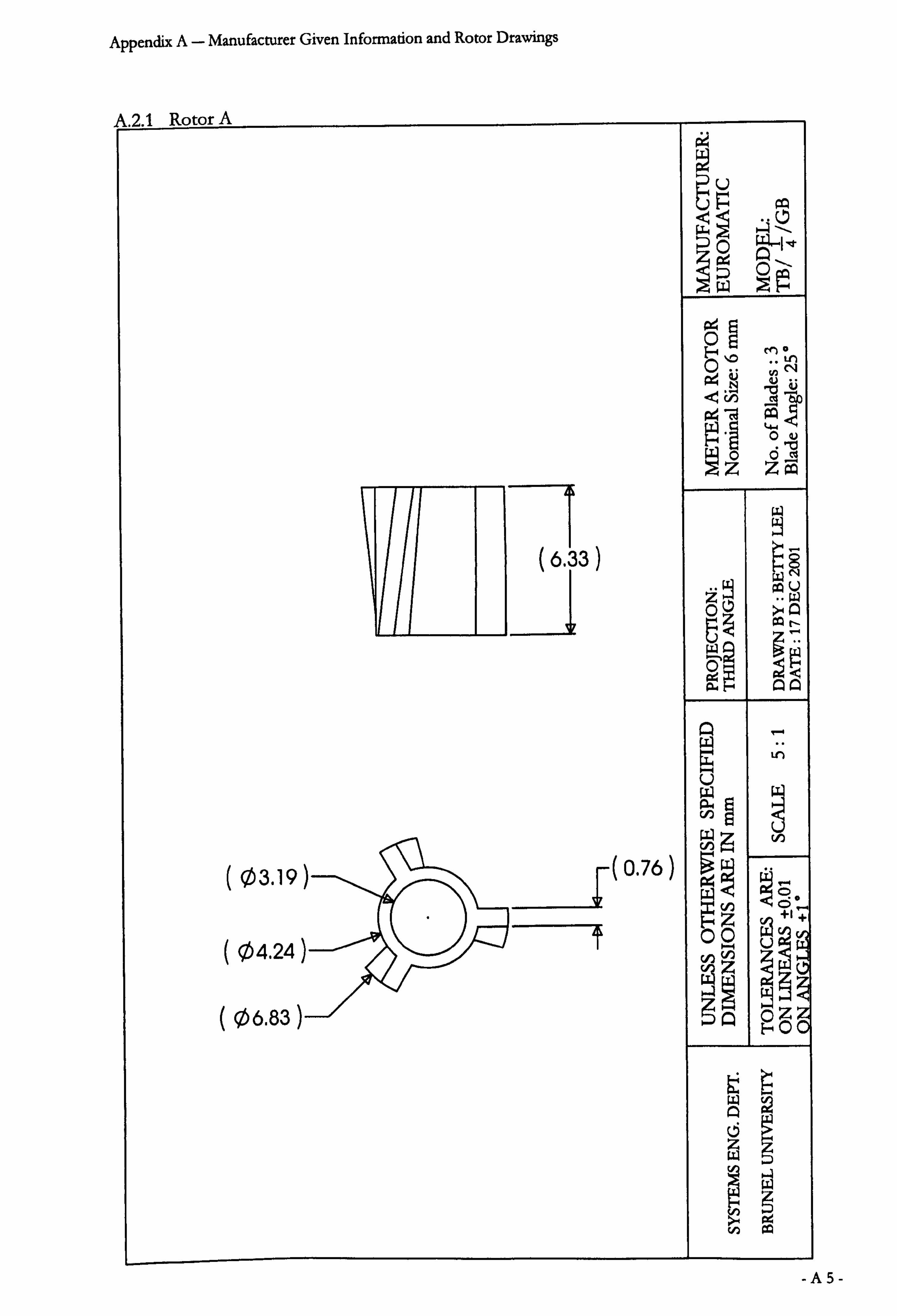
A. 2.1 Rotor A
V PA
Aý wýl
R
MN 41 N
Phi cý :Q
zz
(6.33)
zw
Ow AA
V
U (03.19) (0.76)
L o, Z
°I +
(04.24) 0 ýu
(06.83) . 83) RO
-AS-
Appendix A- Manufacturer Given Information and Rotor Drawings
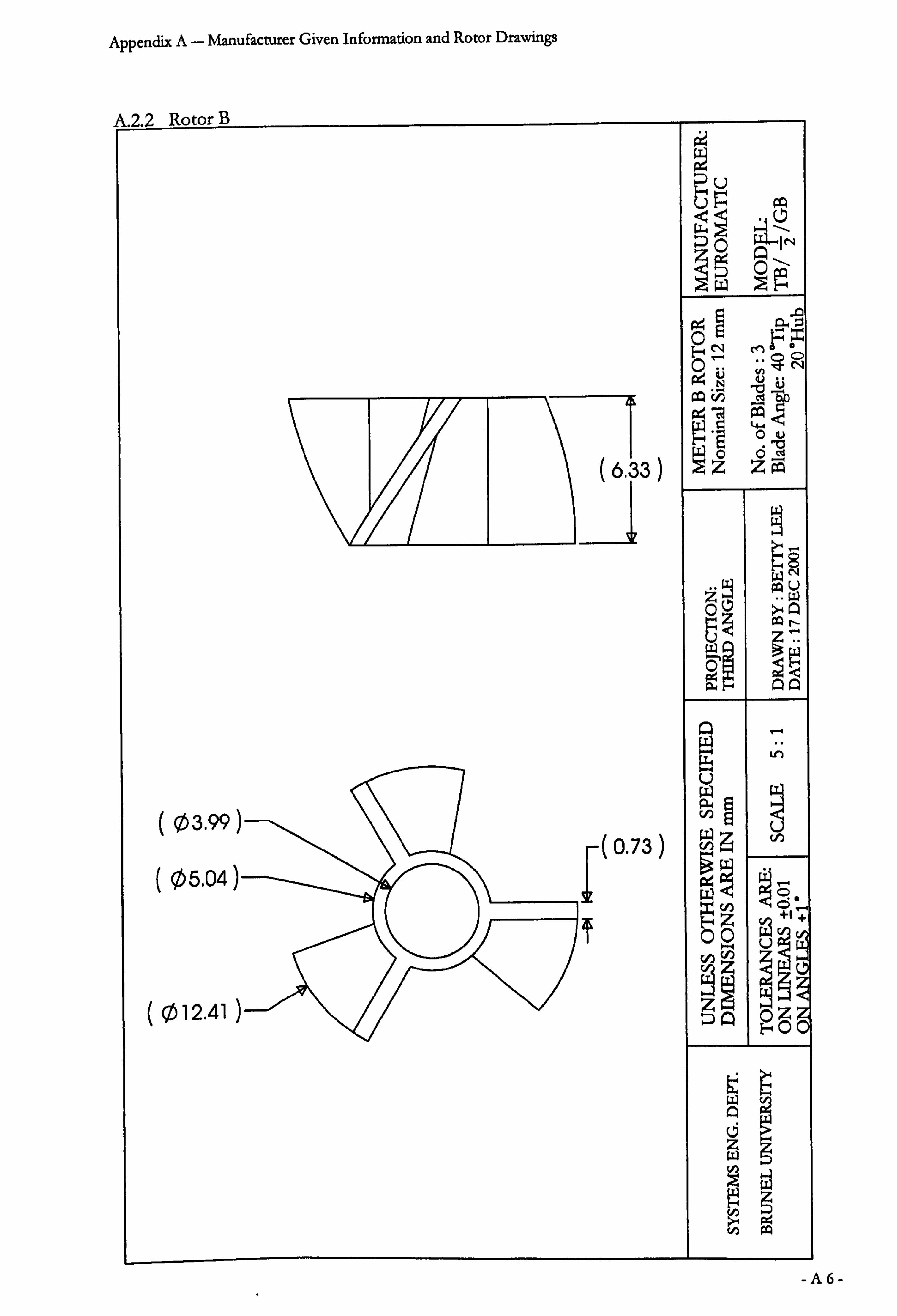
A. 2.2 Rotor 13
V
M
41 ý
CA cn '7u
öA
P4 a 0v
(6.33) ýz ZP
w
zý ýw 00
ä AA
Ln u
3.99 (0.73) 5.4 f
(05.04)
z +1 oo
(012.41) HpÖ
-A6-
Appendix A- Manufacturer Given Information and Rotor Drawings
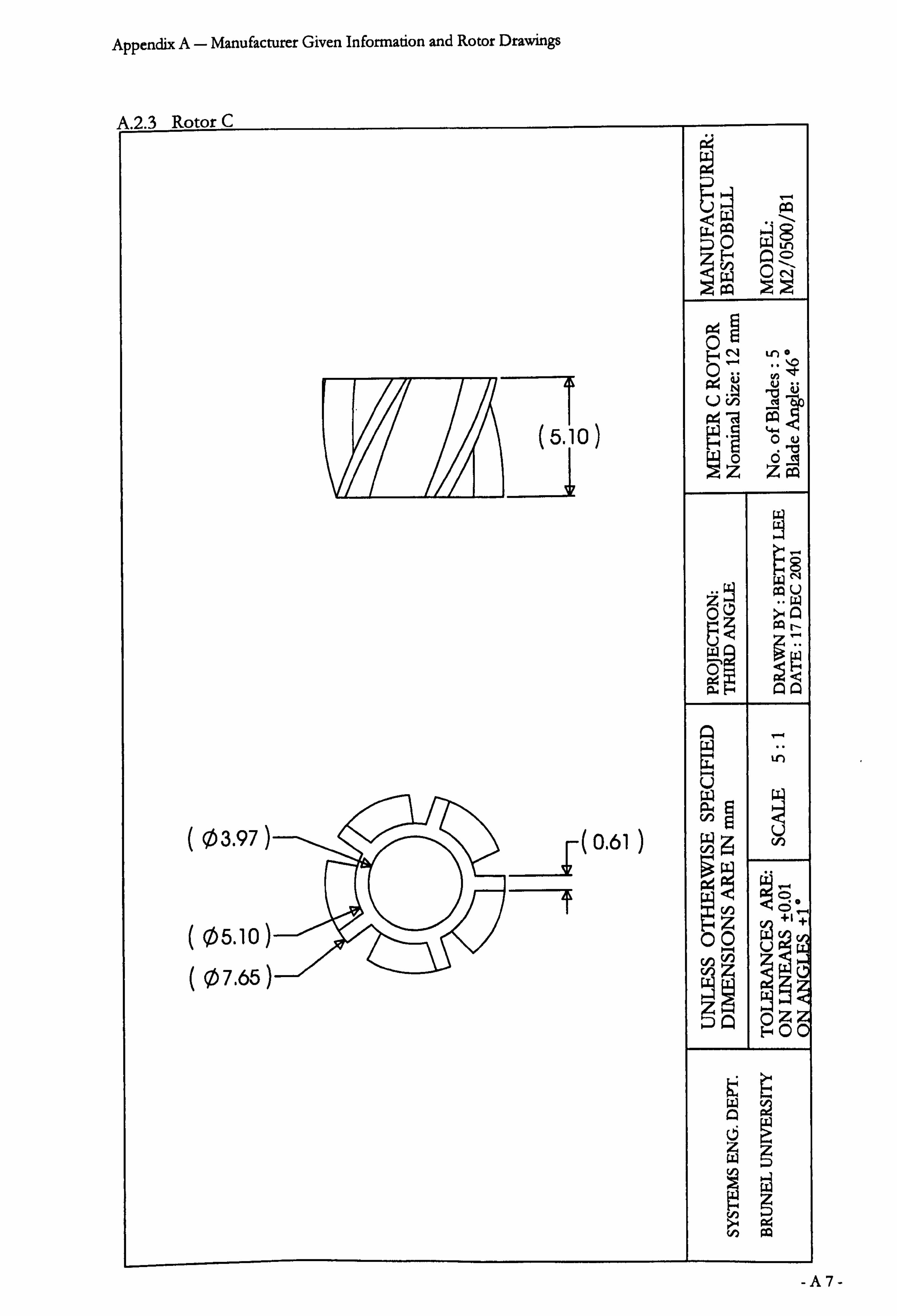
A. 2.3 Rotor C P4
wý äg O Qö
e
(5 0) z 6.1
w 00
ä AÄ
Ü
(03.97) (0.61)
(05.10) 00 0 ý
(07.65) öz Ho
w
vii aha
-A7-
Appendix A- Manufacturer Given Information and Rotor Drawings
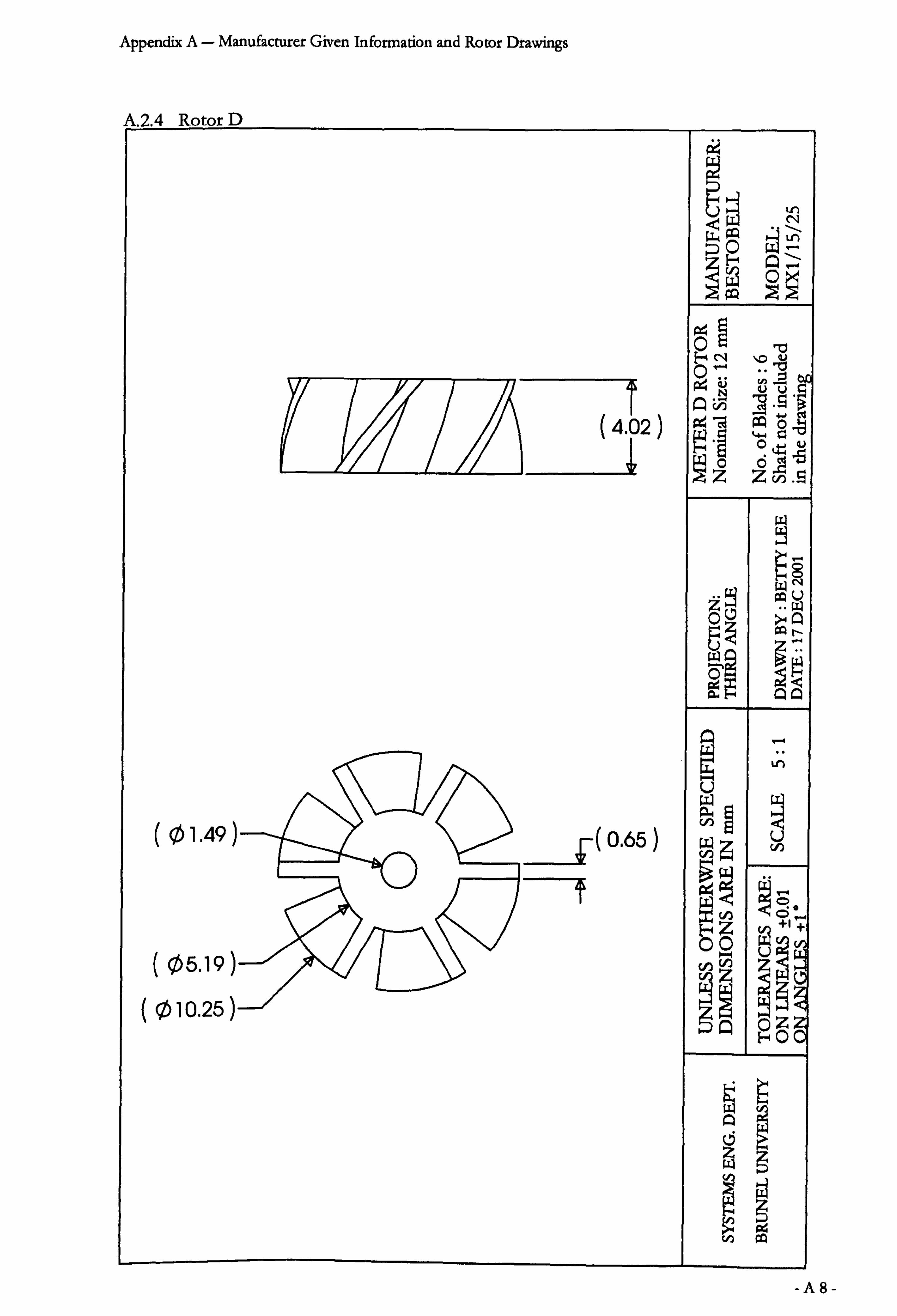
A. 2.4 Rotor D
Ar.
Po,
o
(4.2) VIIA Zz
00 6ý
ä QQ
U
(1,49)
-ý-(0.65) c
Z (05.19)
z
(010.25) oz A H0
wc
-A8-
Appendix A- Manufacturer Given Information and Rotor Drawings
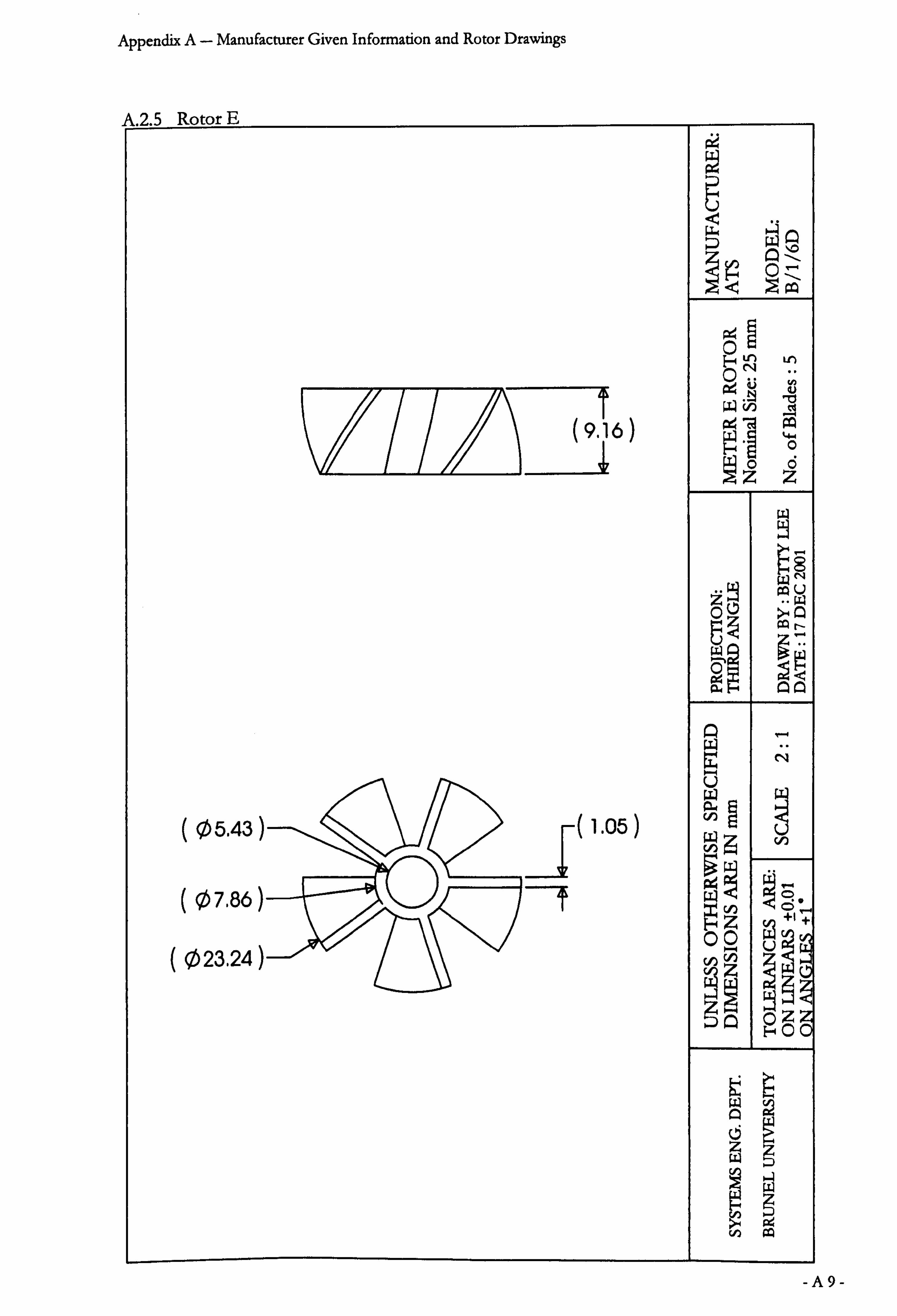
A. 2.5 Rotor E
ý wQ
Oý
N
0. W 'o
(9.16) ö .0 z z
w 00
ä AA
Ü
(05.43) 1(1.05)
ö w" (07.86)
(023.24) 0z
94
°o
-A9-
Appendix B- Step Response Test Method
Appendix B Step Response Test Method
The step response test results (described in Chapter 7.2.1) were obtained by using the
method described by Cheesewright and Clark (1997). As extracted from their paper
(Section 3 "Apparatus for step test experiments"), this section describes the test method
which is of particular relevance to this study.
"The values of the time constant required that for changes in flow to be considered as step
changes would take place over a period of the order of 1 ms. Since the mean velocity of
flow through a typical small turbine meter is several meters per second, it was apparent that
the dynamic pressure forces could be very large. It was therefore decided that any
mechanism controlling the flow would have to be immediately downstream of the meter
and that the supply to the meter would have to be via a pipe having a diameter significantly
greater than that of the meter. The flow was provided by a blow-down system, driven by
compressed air, and the available pressure vessel limited the maximum pressure to 3.5 bar. "
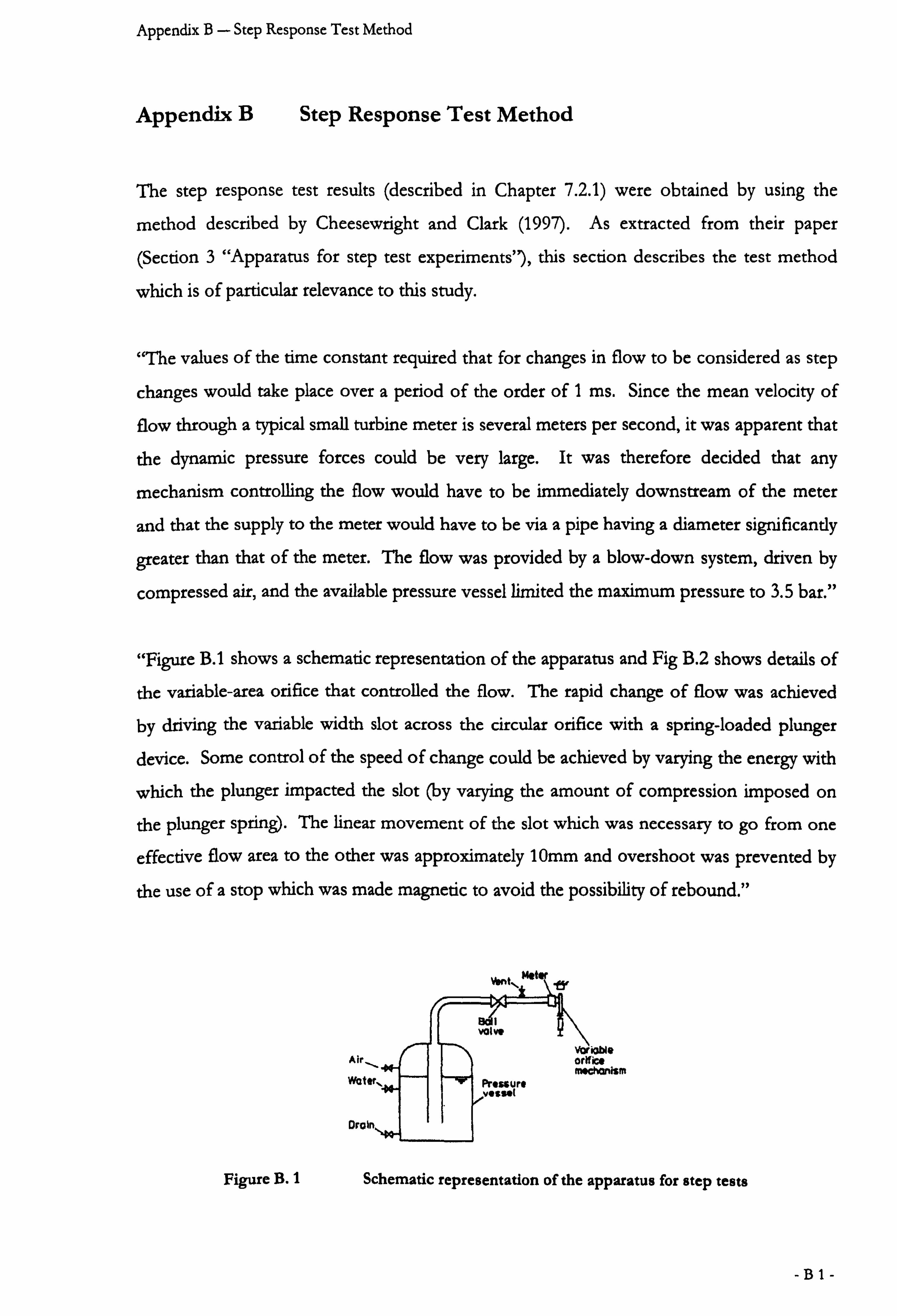
"Figure B. 1 shows a schematic representation of the apparatus and Fig B. 2 shows details of
the variable-area orifice that controlled the flow. The rapid change of flow was achieved
by driving the variable width slot across the circular orifice with a spring-loaded plunger
device. Some control of the speed of change could be achieved by varying the energy with
which the plunger impacted the slot (by varying the amount of compression imposed on
the plunger spring). The linear movement of the slot which was necessary to go from one
effective flow area to the other was approximately 10mm and overshoot was prevented by
the use of a stop which was made magnetic to avoid the possibility of rebound. "
cm
Figure B. 1 Schematic representation of the apparatus for step tests
-B1-
Appendix B- Step Response Test Method
l"Stop
Molar
Variable b wiglh Mot
Plunger
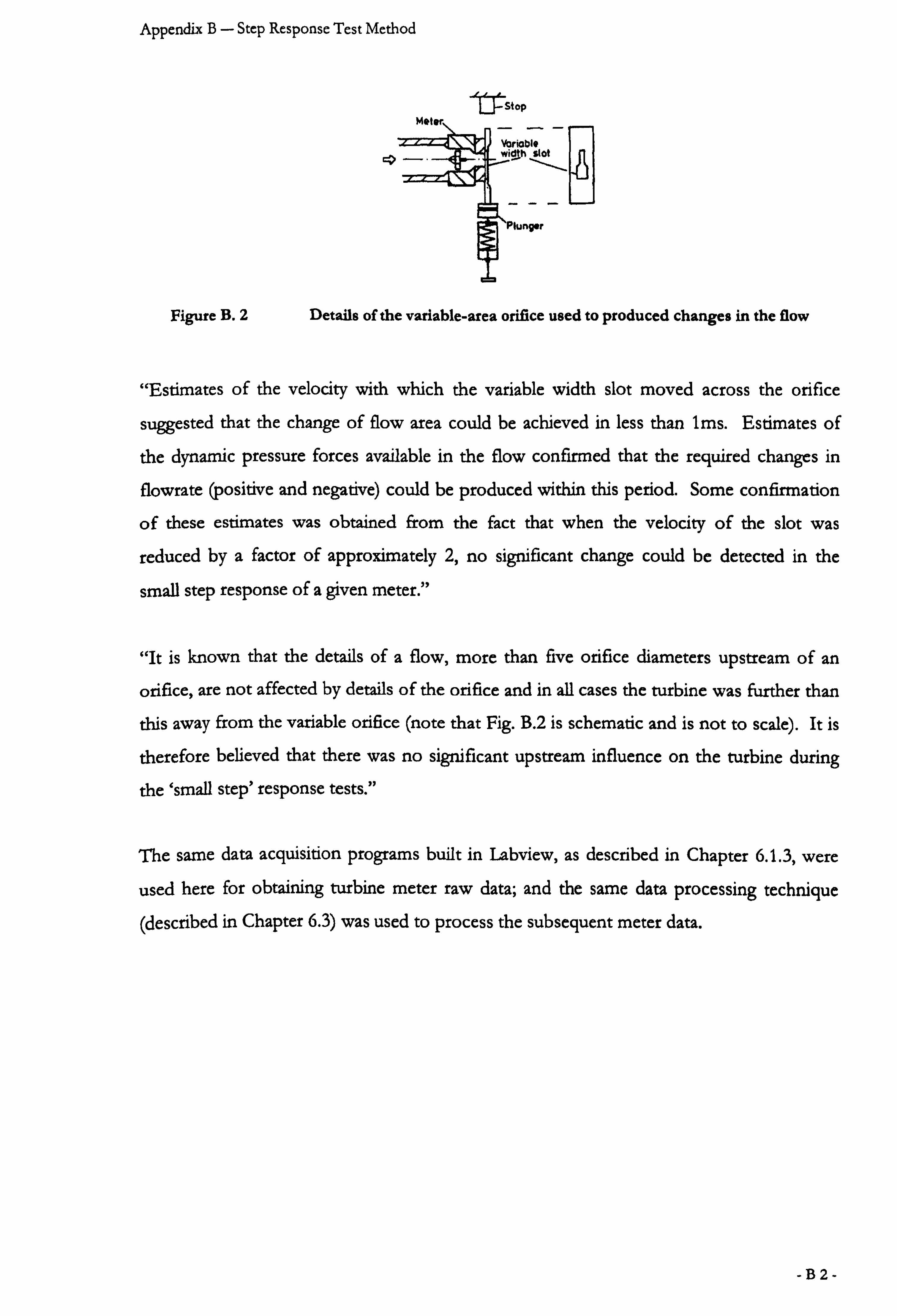
Figure B. 2 Details of the variable-area orifice used to produced changes in the flow
"Estimates of the velocity with which the variable width slot moved across the orifice
suggested that the change of flow area could be achieved in less than 1ms. Estimates of
the dynamic pressure forces available in the flow confirmed that the required changes in
flowrate (positive and negative) could be produced within this period. Some confirmation
of these estimates was obtained from the fact that when the velocity of the slot was
reduced by a factor of approximately 2, no significant change could be detected in the
small step response of a given meter. "
"It is known that the details of a flow, more than five orifice diameters upstream of an
orifice, are not affected by details of the orifice and in all cases the turbine was further than
this away from the variable orifice (note that Fig. B. 2 is schematic and is not to scale). It is
therefore believed that there was no significant upstream influence on the turbine during
the `small step' response tests. "
The same data acquisition programs built in Labview, as described in Chapter 6.1.3, were
used here for obtaining turbine meter raw data; and the same data processing technique
(described in Chapter 6.3) was used to process the subsequent meter data.
-B2-
Appendix C- The Flow Model
Appendix C The Flow Model
CFX provides a solution module that solves the discretised representation of the problem.
A detailed description of the software is given in the Manual. This section is intended to
describe the fundamental mathematical formulations and methods used to depict the flow
behaviour, rather than as a full text. Where appropriate, the equations and their underlying
assumptions are presented in full. In cases where the full equations have been omitted,
references are presented where the analysis and derivations can be found.
C. 1 Governing Equations
The foundation of computational fluid dynamics (CFD) is the fundamental governing
equations of fluid dynamics - the continuity, momentum and energy equations. Since the
fluid flow modelled in this study is assumed to be isothermal, the energy equation is
therefore not considered.
C. 1.1 Continuity equation
The CFX flow solver provides numerical solutions to the Reynolds' averaged Navier
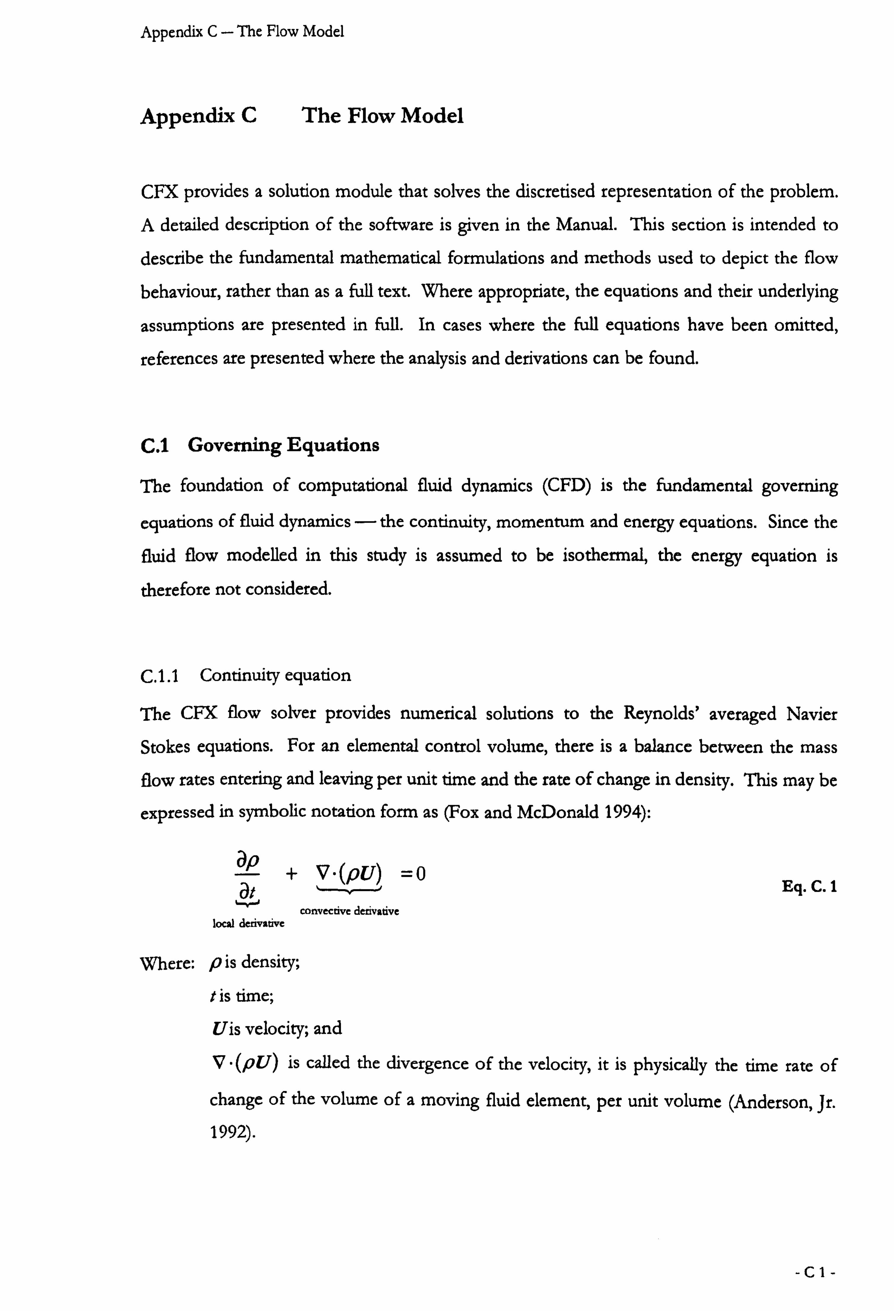
Stokes equations. For an elemental control volume, there is a balance between the mass flow rates entering and leaving per unit time and the rate of change in density. This may be
expressed in symbolic notation form as (Fox and McDonald 1994):
a! ° + V"(pu) =0 Eq. C. 1 at ý-"ý-- ~J
convective derivative local derivative
Where: pis density;
t is time;
Uis velocity; and V" (pU) is called the divergence of the velocity, it is physically the time rate of
change of the volume of a moving fluid element, per unit volume (Anderson, Jr.
1992).
-CI-
Appendix C- The Flow Model
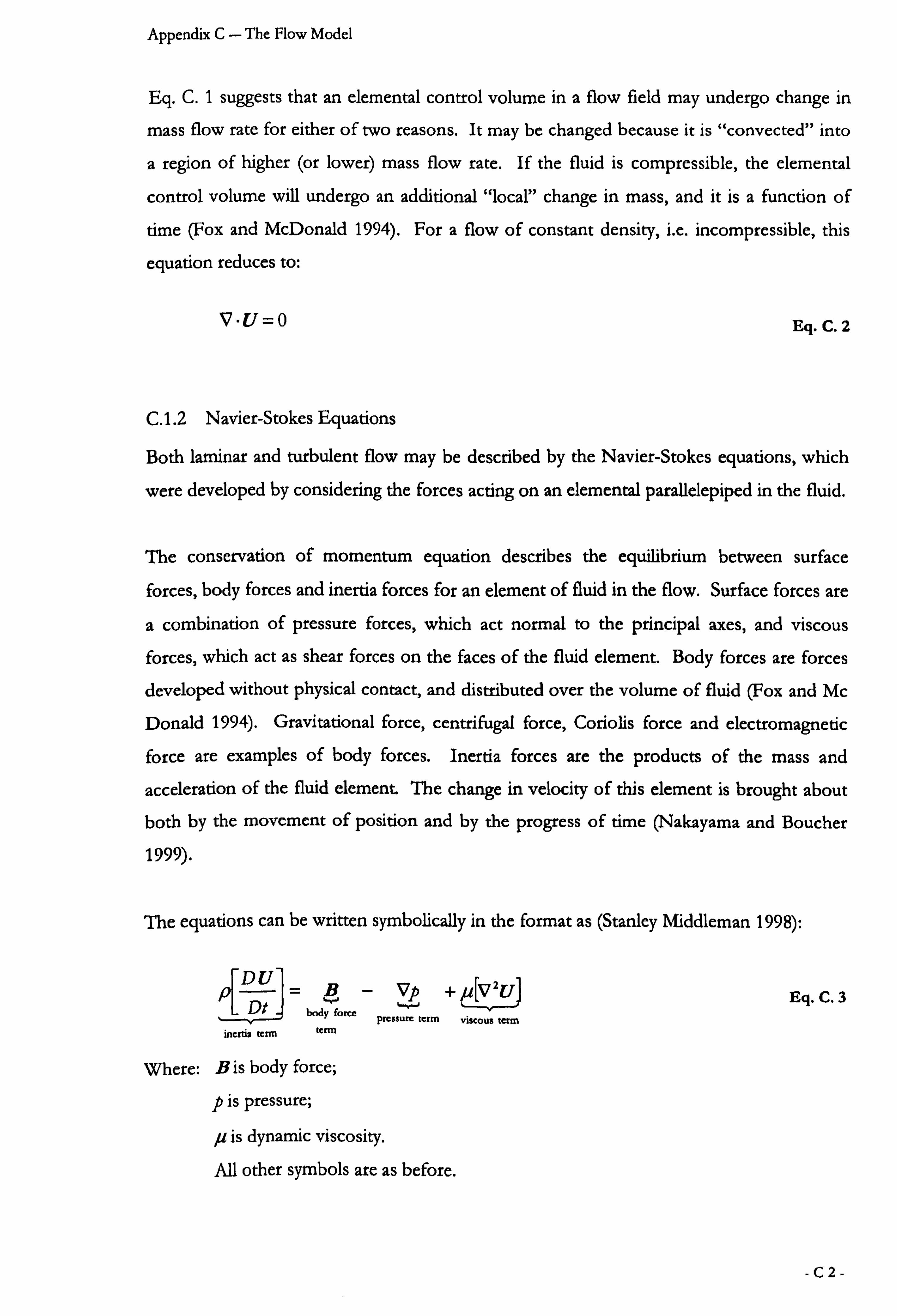
Eq. C. 1 suggests that an elemental control volume in a flow field may undergo change in
mass flow rate for either of two reasons. It may be changed because it is "convected" into
a region of higher (or lower) mass flow rate. If the fluid is compressible, the elemental
control volume will undergo an additional "local" change in mass, and it is a function of
time (Fox and McDonald 1994). For a flow of constant density, i. e. incompressible, this
equation reduces to:
v"U=o
C. 1.2 Navier-Stokes Equations
Eq. C. 2
Both laminar and turbulent flow may be described by the Navier-Stokes equations, which
were developed by considering the forces acting on an elemental parallelepiped in the fluid.
The conservation of momentum equation describes the equilibrium between surface
forces, body forces and inertia forces for an element of fluid in the flow. Surface forces are
a combination of pressure forces, which act normal to the principal axes, and viscous forces, which act as shear forces on the faces of the fluid element. Body forces are forces
developed without physical contact, and distributed over the volume of fluid (Fox and Mc
Donald 1994). Gravitational force, centrifugal force, Coriolis force and electromagnetic
force are examples of body forces. Inertia forces are the products of the mass and
acceleration of the fluid element. The change in velocity of this element is brought about
both by the movement of position and by the progress of time (Nakayama and Boucher
1999).
The equations can be written symbolically in the format as (Stanley Middleman 1998):
DU _B
pC DV body force
inertia term term
- vp +Ao2U pressure term viscous term
Eq. C. 3
Where: Bis body force;
p is pressure;
,u is dynamic viscosity.
All other symbols are as before.
-C2-
Appendix C- The Flow Model
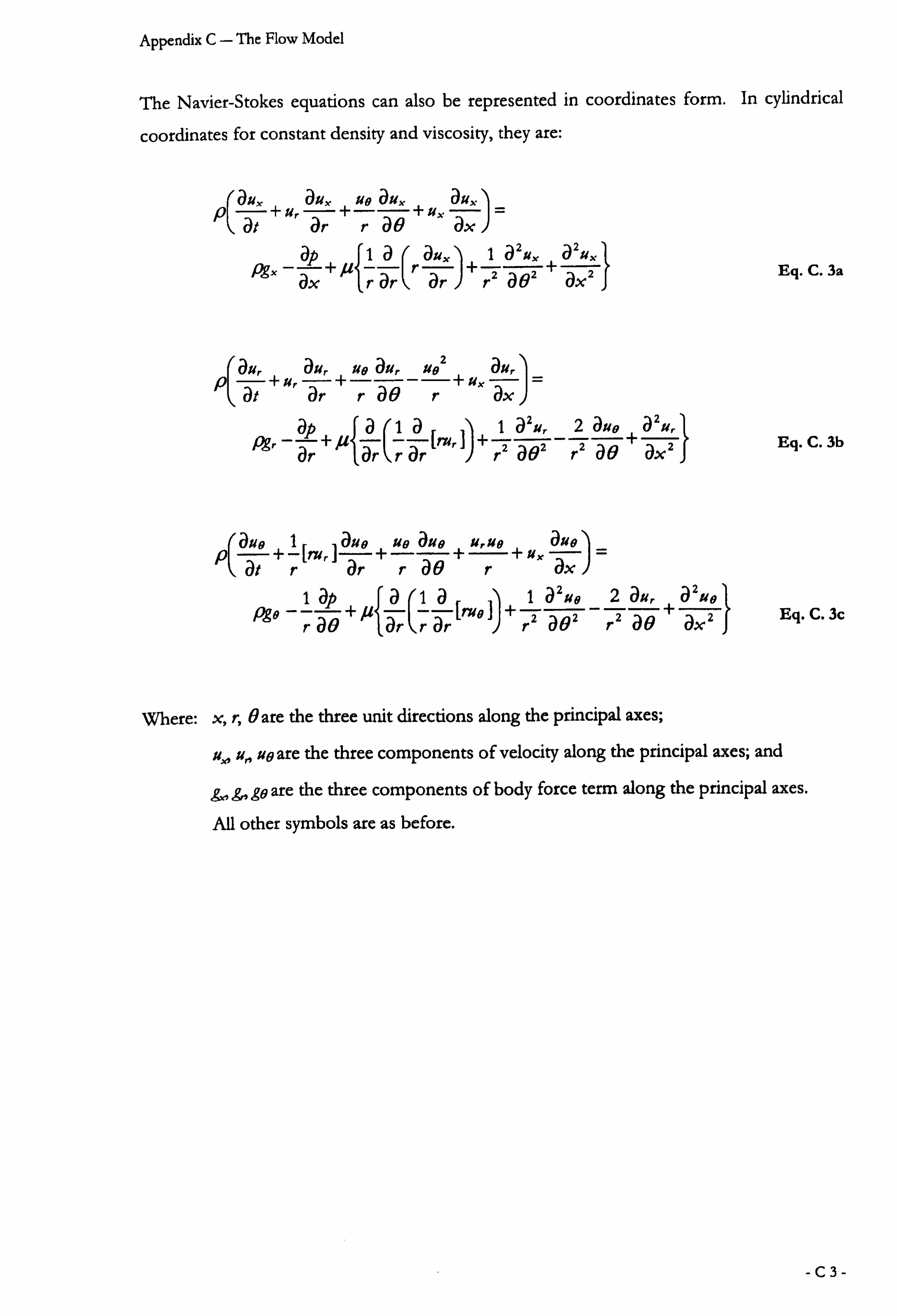
The Navier-Stokes equations can also be represented in coordinates form. In cylindrical
coordinates for constant density and viscosity, they are:
aux +
ue aux au lu-
at + u' ar raO+ ux ax ap 1a au")+ 1 a2ux a2ux
ýx ax
+ rar \r ar r2 ä9Z
+ äx2 Eq. C. 3a
aflr all,. Ug ally U2 auy
0( + Ur
_22 aue a2Ur fr -
ap +, Uý a( 1a 1 lour _ är ar tar kr l
J+ rZ a02 r'2 ae + axZ Eq. C. 3b
auo +1 aue + ue aua + U" U0 + ux tx, 9 pl at r[ ar raBr_
1a pa ý1 a11 ague _2
au, a2u8 ýB
ra8+p--[n B, )+r2 ao2 rZ ae+axe
Eq. C. 3c
Where: x, r, 0 are the three unit directions along the principal axes;
u, u� ue are the three components of velocity along the principal axes; and
gx, g� go are the three components of body force term along the principal axes.
All other symbols are as before.
-C3-
Appendix C- The Flow Model
C. 2 Turbulence Models
The continuity equation and the Navier-Stokes equations described in section C. 1 provide
a full description of the isothermal and incompressible Newtonian flow behaviour of a
fluid element in laminar flow. However, turbulent flows are extremely complex and time-
dependent; since the Navier-Stokes equations are non-linear, coupled and contains partial
differential, it is difficult to solve them to the required accuracy analytically, therefore
turbulence models are used, which solve transport equations for the Reynolds-averaged
quantities.
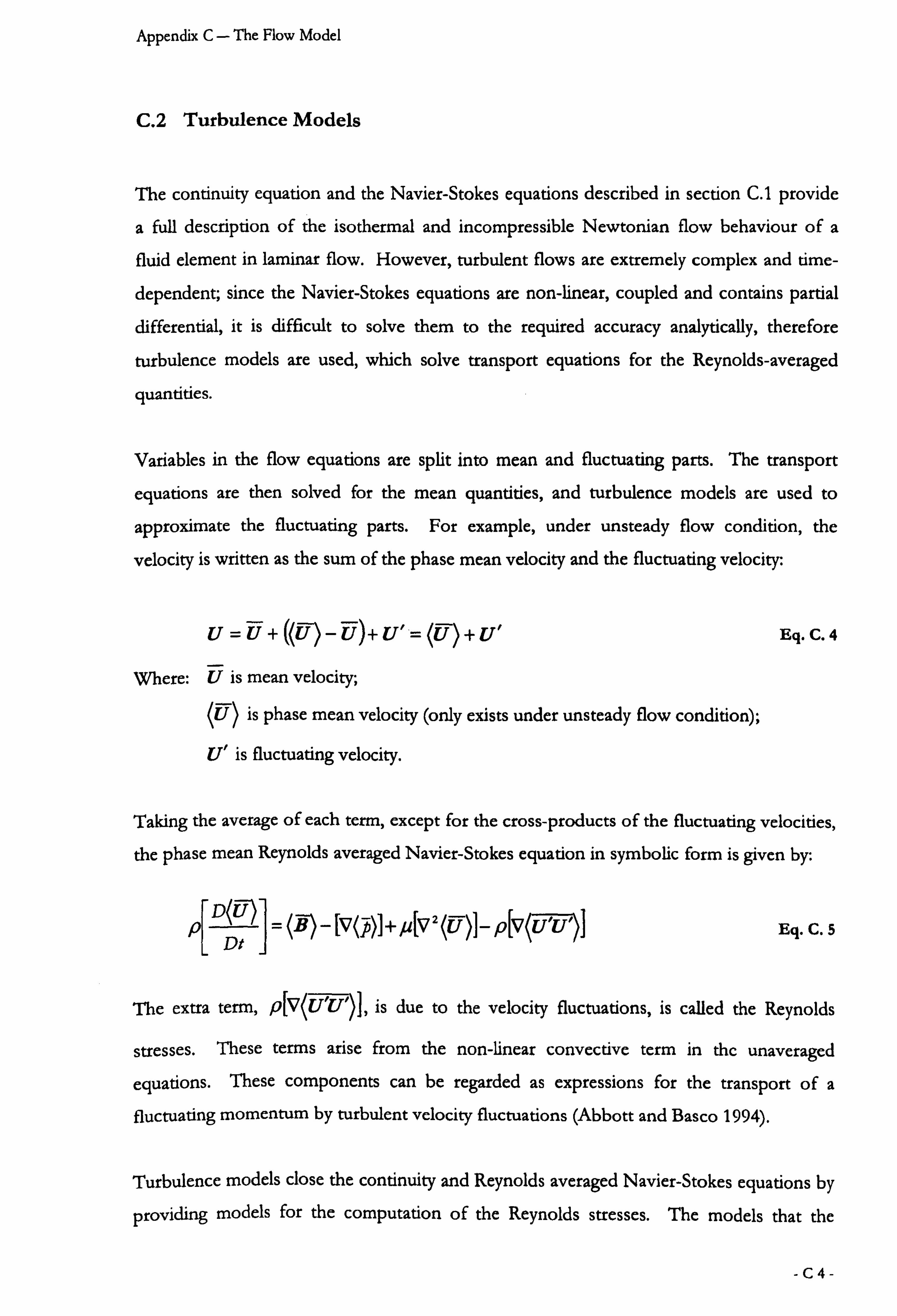
Variables in the flow equations are split into mean and fluctuating parts. The transport
equations are then solved for the mean quantities, and turbulence models are used to
approximate the fluctuating parts. For example, under unsteady flow condition, the
velocity is written as the sum of the phase mean velocity and the fluctuating velocity:
U=U+ýýÜý-Uý+Ul=(U)+ul Eq. C. 4
Where: U is mean velocity;
(U) is phase mean velocity (only exists under unsteady flow condition);
U' is fluctuating velocity.
Taking the average of each term, except for the cross-products of the fluctuating velocities,
the phase mean Reynolds averaged Navier-Stokes equation in symbolic form is given by:
D(U) [v(p)] +, U[V2(U)]-pII UUJ Eq. C. 5 Dt
The extra term, p[V(UV)I, is due to the velocity fluctuations, is called the Reynolds
stresses. These terms arise from the non-linear convective term in the unaveraged
equations. These components can be regarded as expressions for the transport of a
fluctuating momentum by turbulent velocity fluctuations (Abbott and Basco 1994).
Turbulence models close the continuity and Reynolds averaged Navier-Stokes equations by
providing models for the computation of the Reynolds stresses. The models that the
-C4-
Appendix C- The Flow Model
solver provides can be put into two broad classes: eddy viscosity models and second order
closure models.
Eddy viscosity models solve the Reynolds stresses and fluxes algebraically in terms of
known mean quantities. The eddy viscosity hypothesis is that the Reynolds stresses can be
linearly related to the mean velocity gradients in a manner analogous to the relationship
between the stress and strain tensors in laminar Newtonian flow. These models are
distinguished by the manner in which they prescribe the eddy viscosity and eddy diffusivity.
Examples are k-E model, low Reynolds number k-C model and RNG k-E model. The low
Reynolds number model is the modification of the standard models to allow calculation of
turbulent flows at low Reynolds number, typically in the range 5,000 to 30,000. Since we
aim to solve to the laminar boundary layer of blade surfaces in which the local Reynolds
number is around 20,000 (see section C. 3.3), therefore low Reynolds number k-E model
was chosen to be the prime model for this research case.
Second order closure models solve differential transport models for the turbulent fluxes,
which have to be modelled in terms of known lower order ones. These types of models
are often called Reynolds stress models. The advantage of doing this over the methods
mentioned previously is that those methods give a single additional viscosity, whereas the
direct modelling of the stress terms allows the effects of turbulence to vary in the three
coordinate directions. Eddy viscosity models are said to give isotropic turbulence, in which
turbulence is assumed to be constant in all directions, whereas in the real situation the
turbulence is said to be anisotropic (Shaw 1992). However, low Reynolds number versions
of these models were not available within the solver. Therefore, no further description of
these models will be presented here.
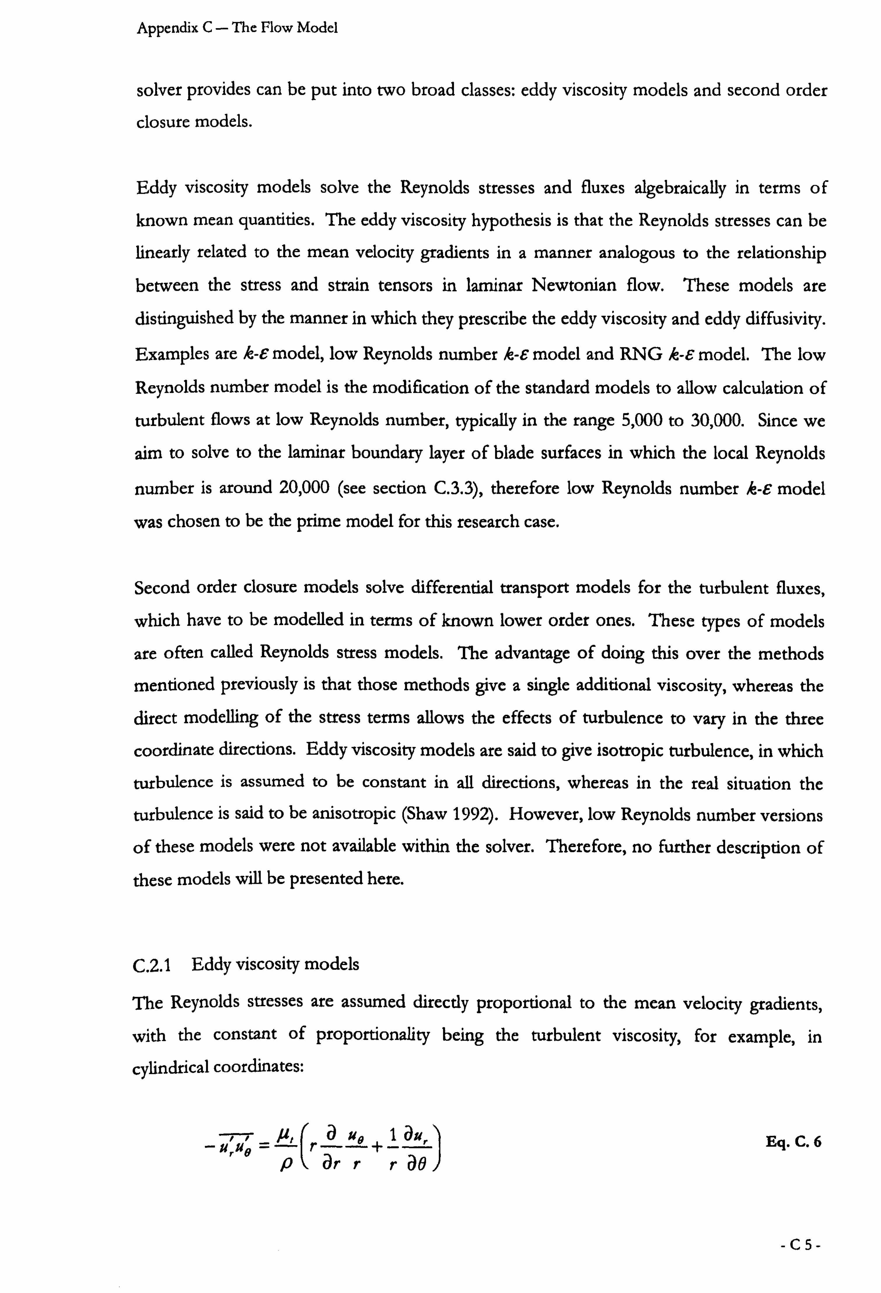
C. 2.1 Eddy viscosity models
The Reynolds stresses are assumed directly proportional to the mean velocity gradients,
with the constant of proportionality being the turbulent viscosity, for example, in
cylindrical coordinates:
UrUO 'u` rB+ 1äu,
q auEC.
6 p ar rr aO
-C5-
Appendix C- The Flow Model
Where: p, is the turbulent viscosity;
r, 9 are the unit directions along the principal axes;
ur, ue are the components of velocity along the principal axes;
ü,, ue are the components of fluctuating velocity.
All other symbols are as before.
The turbulent viscosity is not a value of a physical property dependent on the temperature
or such, but a quantity fluctuating according to the flow condition (Nakayama and Boucher
1999):
Z ýr = Cup
k Eq. C. 7
where: C,, is a constant;
k is the turbulent kinetic energy (note it has units of velocity squared);
E is the rate of dissipation of turbulent kinetic energy
Turbulent transport will have a substantial effect on boundary layer development within a
turbine flowmeter. CFX 4.3 incorporates a range of models for turbulent transport
suitable for use in engineering calculations. A brief summary of three of the available
turbulence models, which were considered in preliminary investigations, is presented
below.
C. 2.1.1 k-E model
The standard k-E model (Launder and Spalding 1974) uses an eddy-viscosity hypothesis for
the turbulence. In addition to the mean flow equations, it solves separate transport
equations for both turbulent kinetic energy, k, and the rate of dissipation of turbulent
kinetic energy, e for use in Eq. C. 7 to determine A. At any point in the flow this same A
is used in all flow directions, i. e. for all Reynolds stress components. This usage is
equivalent to the assumption of a local isotropy in the turbulence (Abbott and Basco 1994).
Both equations have the same form; the rate of change of k or e is related to the convective
and diffusive transport and the production and dissipation. Resorting to vector notation,
the equations are written as:
-C6-
Appendix C- The Flow Model
päk+0"(pUk)=P+B-pE+V" , u+E` Vk Eq. C. 8
, oae+V. (JOUE)=c, F(P+c3B)-C210IF +v" /J+ý ve at kkQ1 Eq. C. 9
Where: C,, C2, O rk, O. are model constants,
Pis the shear production, defined below
All other symbols are as before.
P=(fU +p, )OU. (VU+(VU)T)-2VU((fu +Fu ,
)OU+pk) Eq. C. 1O
The constants in these equations have been developed following studies of a wide range of
turbulent flows.
This model is not suitable for solution in the near wall region of a boundary layer. Where
such a solution is required the model may be used in combination with a wall function to
bridge the near wall region calculation.
C. 2.1.2 Low Reynolds number k-E model
CFX Flow Solver provides this particular turbulent model developed by Launder and
Sharma (1974), it is a modification of the standard k-e model to allow calculation of
turbulent flows at low Reynolds number, typically in the range 5000 to 30000. The model
involves a damping of the turbulent viscosity when the local turbulent Reynolds number is
low, a modified definition of E so that it goes to zero at walls and modifications of the
source terms in the 6 equation. The equations are integrated to the wall through the
laminar sublayer.
Practically all incompressible turbulence models invoke the large Reynolds number (Re)
assumption, thus allowing the effects of viscosity to be neglected as a first approximation.
This assumption has its drawback as the flow Re decreases or as a wall is approached. In
-C7-
Appendix C- The Flow Model
both cases, the effective Re of the flow becomes smaller. However, there is a distinct
difference between the two situations even though the effective flow Re is the same. For
flows in an infinite medium, there are no walls and decreasing Re introduces viscous effects
only. On the other hand, the local Re decreases as a wall is approached and, in addition,
the wall reflects the fluctuating pressure and thus contributes to an increased anisotropy of
the turbulence field near the wall. This effect is commonly known as wall blocking.
Therefore, near-wall turbulence includes both viscous and blocking effects while low-Re
turbulence consists of viscous effects alone (Speziale and So 1998).
The equations describing the turbulence model: Eq. C. 7, Eq. C. 8 and Eq. C. 9 become:
ýf = CIlf-p kZ
Eq. C. 11
päk+V-(pUk)=P+B-pe+V. u+E` Vk -D Eq. C. 12 k
ae +v ve-c e (P+c B)-c f ýZ +v- +ý`ý VE +E Eq. C. 13 P ýt (P )- k3z', k E
Here the definition of Pis changed slightly from Eq. C. 10 to use A only instead of (y+, u).
The functions fý, fý, D and E are defined by:
ex -3.4 Eq. C. 14 f" p
1+(R,. /50)2
f2= 1-0.3 exp( RT2) Eq. C. 15
D=2p(Vkyy Eq. C. 16
E=2'uß` (VV U)2 Eq. C. 17
where the local turbulent Reynolds number is defined by:
_pkz RT - jue
Eq. C. 18
-C8-
Appendix C- The Flow Model
C. 2.1.3 RNG k-E model
RNG k-e model is an alternative to the standard k-E model for high Reynolds number
flows. It derives from a renormalization group analysis of the Navier-Stokes equations and
differs from the standard model only through a modification to the equation for e, except
for using a different set of model constants.
The RNG model has not been as widely validated as the k-E model. However, it has been
shown to give better results for many flow regimes, particularly the highly turbulent flows
common in wind engineering applications. According to Caffrey et al (1997), the RNG
model can give superior results for swirling flows.
Summary:
In the present study, negligible swirling flow is assumed due to the effect of upstream and
downstream flow straighteners. And the interest only lies on solving the hydrodynamic
forces acting on the localised region of the rotor blading when the meter is subjected to
pulsating flow conditions. This implies that the blade wall boundary layer flow simulation
is of most importance. In view of this, as the local Reynolds number of the blade, Re, is
around 20000 within the flow regime (See C. 3.3), Low Re number k-e model was chosen
to be the turbulent model for this particular flow problem.
-C9-
Appendix C- The Flow Model
C. 3 Mathematical Details on Boundary Conditions
C. 3.1 Inlet Boundary
Assuming that the whole volume flow goes through the annular flow passage, the inlet
velocity (freestream) can simply be inferred from the following formula:
Inlet Velocity = Volume Flowrate + Annular Cross - section Area
U� =V +A Eq. C. 19
The value of inlet velocity is calculated based on the experimental flow condition, in which
the mean flowrate is 0.292x10"3 m3/s for this meter (See Chapter 6). Knowing the values
of the casing radius (r) and hub radius (r), the annular area is calculated by using the
following equation:
A =, r(rr2 - rr2 )
=''(1.293x10⁻² )2 - 5.04x10⁻³)2j
=1.113X10-'m2
Now, by using Eq. C. 19, the inlet freestream mean velocity is:
U- =0.292x10-'m'/s+1.113x1O m2
= 2.629 m/s
Eq. C. 20
For steady flow condition, the above value is input into the solver. For unsteady flow
condition, pure sinusoidal pulsating flow is assumed. With ap being the relative pulsation
amplitude and fy being the pulsation frequency, the velocity will be time dependent
periodically as follows:
Um (t) = U-, (i +ap sin 2ýf t) Eq. C. 21
The above equation is then input into Fortran subroutine, USRBCS, for the calculation of boundary condition at the inlet for unsteady flow runs.
-cio-
Appendix C- The Flow Model
The values of the inlet turbulence quantities are based upon the characteristic of a fully
developed pipe flow. The equations for the inlet values of turbulent kinetic energy, k, is:
k 2u, 2 Eq. C. 22
where u, is the shear stress velocity, (= r ,p), in which Z, is the wall shear stress.
Introducing a dimensionless skin-friction coefficient, C1:
Cf= Z"
Eq. C. 23 pU-, 2
uT = Cl /2 }II� Eq. C. 24
According to Blausius' approximate solution for laminar flow over flat plate using
sinusoidal velocity profile, the skin-friction coefficient, Cf= 0.664(Re)"2 (Massey 1992).
Taking the local Reynolds number. to be equivalent to the pipe Reynolds number, for this
flow condition, Re, = Red = 3.11x10`, hence Cf = 3.765x10"3. By substituting this value
into Eq. C. 24, u, is equal to 0.115 and hence k is approximated to be 0.026 m2/s2.
The rate of dissipation of turbulent kinetic energy, e, are
k 1.5
0.3D Eq. C. 25
D is the hydraulic diameter of the domain, which is approximated to 0.0125m.
C. 3.2 Outlet Boundary
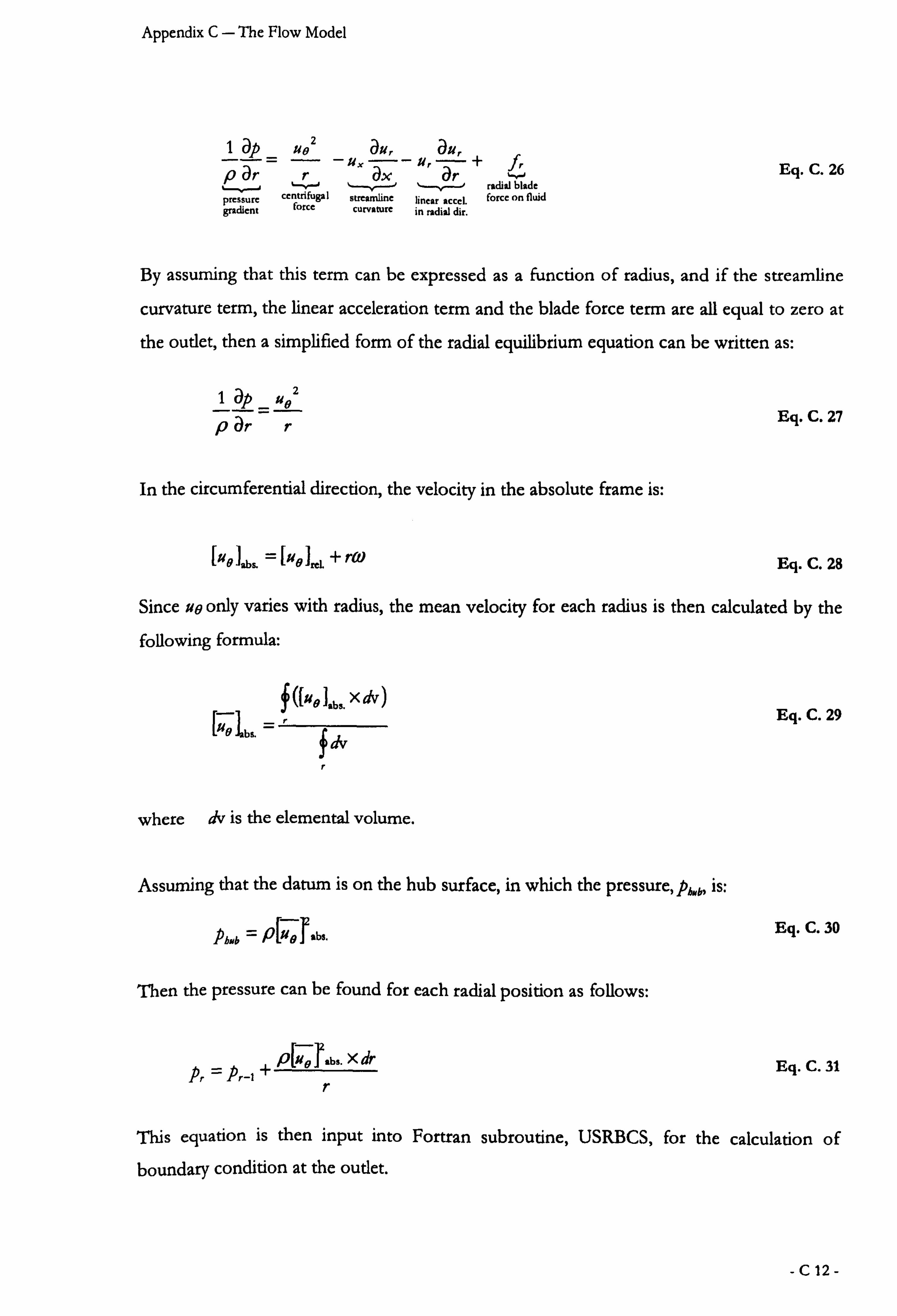
According to Wisler 1998, in order to determine radial variations in vector diagrams and
flow properties, it is critical that the pressure gradients, momentum changes, and blade
forces on the fluid be balanced in the radial direction. The radial equilibrium equation is
formulated from the momentum equation (Eq. C. 3b) for the r component of velocity as
shown below. The assumption of axial symmetry has eliminated terms containing
variations in the tangential direction 0
-CI1-
Appendix C- The Flow Model
lap U01 au,. au,
par r -uX- ax - ur-+ Tr Jr
Eq. C. 26 radial blade
pressure centrifugal streamline linear accel. force on fluid gradient
force curvature in radial dir.
By assuming that this term can be expressed as a function of radius, and if the streamline
curvature term, the linear acceleration term and the blade force term are all equal to zero at
the outlet, then a simplified form of the radial equilibrium equation can be written as:
1 öp _
ue2 Eq. C. 27
p ör r
In the circumferential direction, the velocity in the absolute frame is:
lublabs. _
[ue 1", + rw Eq. C. 28
Since ue only varies with radius, the mean velocity for each radius is then calculated by the following formula:
_
([u9 Jabs.
x dv_
Eq. C. 29
r
where dv is the elemental volume.
Assuming that the datum is on the hub surface, in which the pressure, pld, is:
Ybub - plus
fbs" Eq. C. 30
Then the pressure can be found for each radial position as follows:
Yr = Yr-t
+ P[ cabs. X dr
Eq. C. 31
r
This equation is then input into Fortran subroutine, USRBCS, for the calculation of boundary condition at the outlet.
-C12-
Appendix C- The Flow Model
C. 3.3 Wall Boundaries
As an illustration, this section shows the procedure in establishing the value of d, distance
between the wall and centre of the first grid, of the blade wall surrounding grid.
Firstly, the boundary layer characteristic has to be known. The local Reynolds number,
Re,, of the blade is:
Re, = PU°°c
=1.761x10⁴ Eq. C. 32 I"
Where the blade chord, cis 6.740X1 0"3m, all other values are as before.
According to Blasius, for a flat plate, if Re, <5x 10⁵, it represents a laminar boundary layer
on a flat plate with zero pressure gradient.
In the region very close to the wall where viscous shear is dominant, the mean velocity
profile follows the below linear viscous relation:
pusd Eq. C. 33 9
where d is distance measured from the wall. All other notations are as before.
By substituting Eq. C 24 into Eq. C. 33;
Y+= __ Cfl2
Eq. C. 34 I"
According to Blausius' approximate solution for laminar flow over flat plate using
sinusoidal velocity profile, the skin-friction coefficient, Cf= 0.664(Re)"'/2 (Massey 1992).
Subsequent to computing Re/, Cf = 5.004x10"3. Rearranging the above equation, if y+ = 0.3,
d has a value of:
d= y+'u = 2.294x10⁻⁶m
pU� Cf /2
The same calculation was done to define the distance of first node centre from hub and
casing surfaces by using ay+ value of 30.
-C13-
Appendix C- The Flow Model
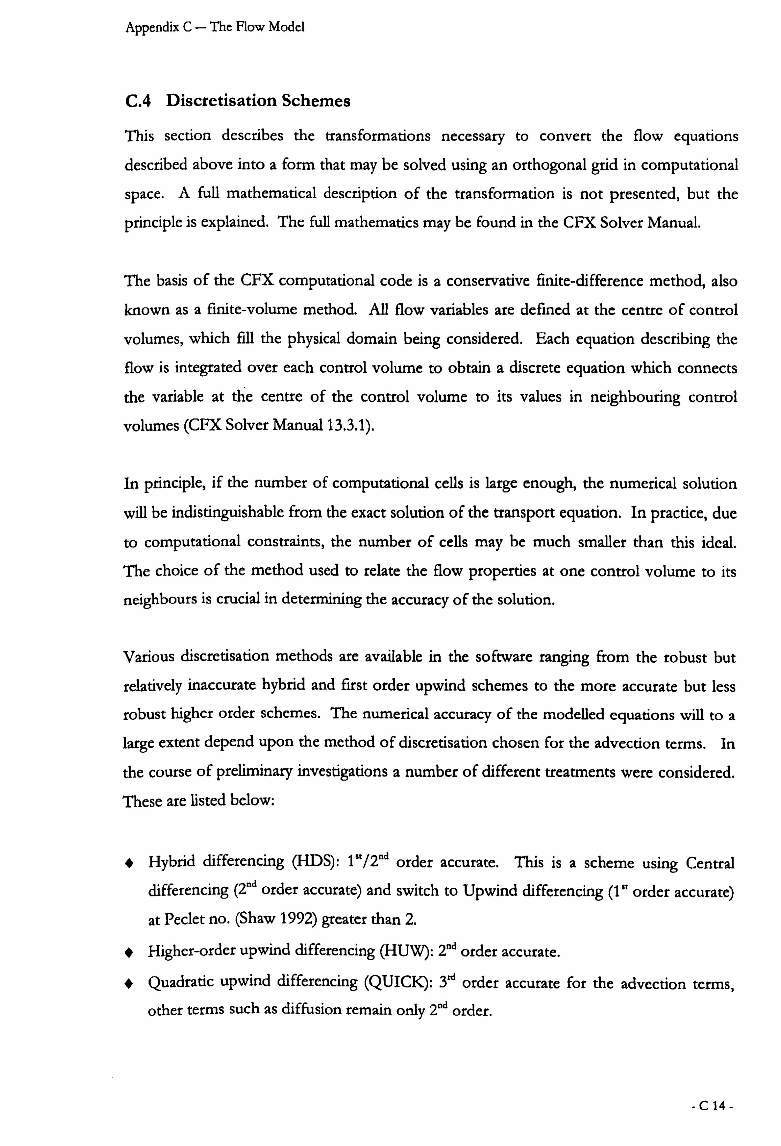
C. 4 Discretisation Schemes
This section describes the transformations necessary to convert the flow equations
described above into a form that may be solved using an orthogonal grid in computational
space. A full mathematical description of the transformation is not presented, but the
principle is explained. The full mathematics may be found in the CFX Solver Manual.
The basis of the CFX computational code is a conservative finite-difference method, also known as a finite-volume method. All flow variables are defined at the centre of control
volumes, which fill the physical domain being considered. Each equation describing the
flow is integrated over each control volume to obtain a discrete equation which connects
the variable at the centre of the control volume to its values in neighbouring control
volumes (CFX Solver Manual 13.3.1).
In principle, if the number of computational cells is large enough, the numerical solution
will be indistinguishable from the exact solution of the transport equation. In practice, due
to computational constraints, the number of cells may be much smaller than this ideal.
The choice of the method used to relate the flow properties at one control volume to its
neighbours is crucial in determining the accuracy of the solution.
Various discretisation methods are available in the software ranging from the robust but
relatively inaccurate hybrid and first order upwind schemes to the more accurate but less
robust higher order schemes. The numerical accuracy of the modelled equations will to a
large extent depend upon the method of discretisation chosen for the advection terms. In
the course of preliminary investigations a number of different treatments were considered.
These are listed below:
f Hybrid differencing (HDS): 1°`/2"a order accurate. This is a scheme using Central
differencing (2"d order accurate) and switch to Upwind differencing (1" order accurate)
at Peclet no. (Shaw 1992) greater than 2.
f Higher-order upwind differencing (HUW): 2 "d order accurate.
f Quadratic upwind differencing (QUICK): 3`d order accurate for the advection terms,
other terms such as diffusion remain only 2 °d order.
-C14-

Appendix C- The Flow Model
f CCCT: 3`d order accurate. In particular, the higher order upwinded schemes can suffer
from non-physical overshoots in their solutions. For example, turbulent kinetic energy
can become negative. CCCT is a modification of the QUICK scheme which is
bounded, eliminating these overshoots.
The more accurate the schemes tend to be less robust and slower (CFX Solver Manual). In
view of this, CCCT was chosen to be the main discretisation scheme used in the flow
modelling for an optimal accurate solution. Whilst, if a solution is difficult to achieve (or
the solver tends to fail in a particular case), Hybrid differencing scheme was used instead
for the k and 6 equations.
-C15-
Appendix C- The Flow Model
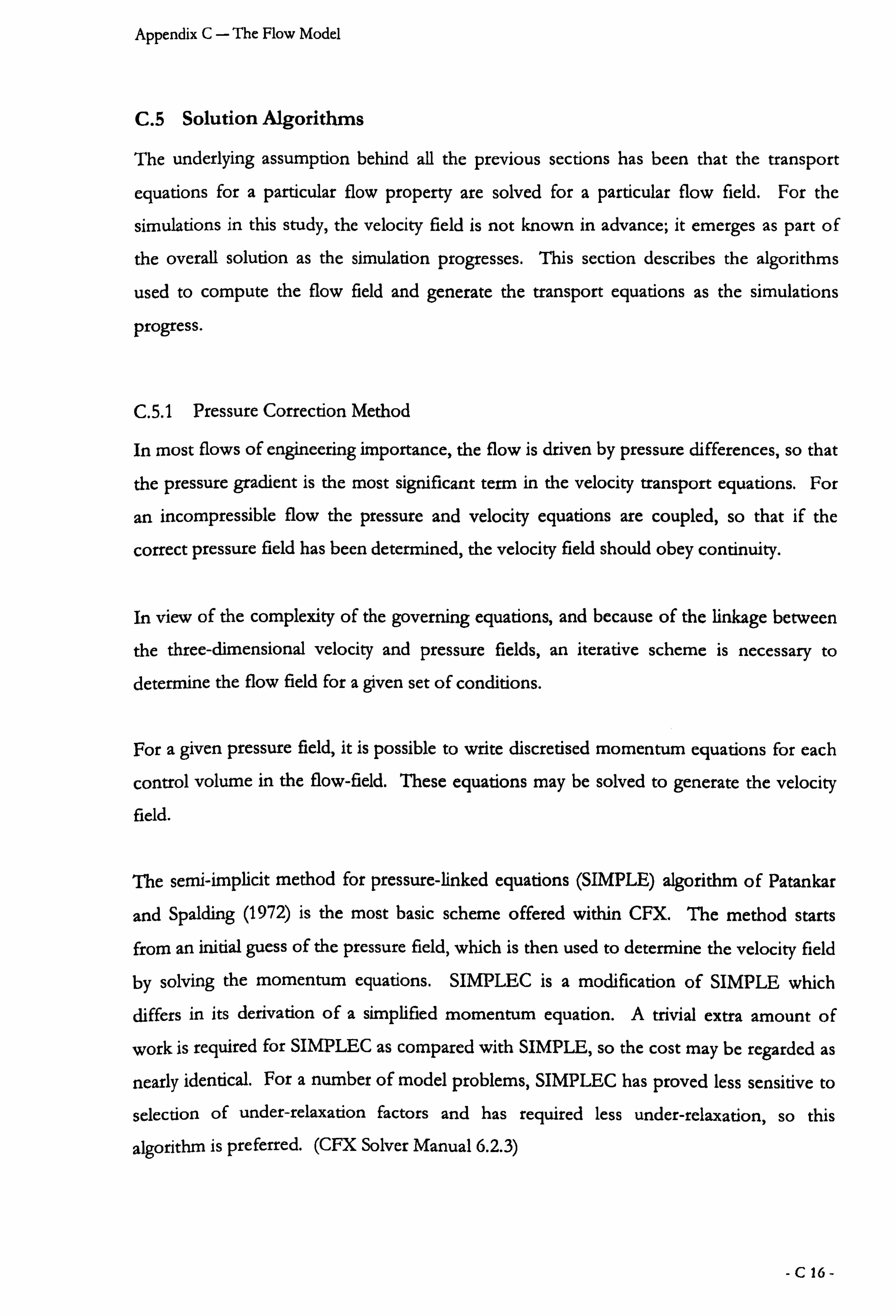
C. 5 Solution Algorithms
The underlying assumption behind all the previous sections has been that the transport
equations for a particular flow property are solved for a particular flow field. For the
simulations in this study, the velocity field is not known in advance; it emerges as part of
the overall solution as the simulation progresses. This section describes the algorithms
used to compute the flow field and generate the transport equations as the simulations
progress.
C. 5.1 Pressure Correction Method
In most flows of engineering importance, the flow is driven by pressure differences, so that
the pressure gradient is the most significant term in the velocity transport equations. For
an incompressible flow the pressure and velocity equations are coupled, so that if the
correct pressure field has been determined, the velocity field should obey continuity.
In view of the complexity of the governing equations, and because of the linkage between
the three-dimensional velocity and pressure fields, an iterative scheme is necessary to
determine the flow field for a given set of conditions.
For a given pressure field, it is possible to write discretised momentum equations for each
control volume in the flow-field. These equations may be solved to generate the velocity field.
The semi-implicit method for pressure-linked equations (SIMPLE) algorithm of Patankar
and Spalding (1972) is the most basic scheme offered within CFX. The method starts
from an initial guess of the pressure field, which is then used to determine the velocity field
by solving the momentum equations. SIMPLEC is a modification of SIMPLE which differs in its derivation of a simplified momentum equation. A trivial extra amount of
work is required for SIMPLEC as compared with SIMPLE, so the cost may be regarded as
nearly identical. For a number of model problems, SIMPLEC has proved less sensitive to
selection of under-relaxation factors and has required less under-relaxation, so this
algorithm is preferred. (CFX Solver Manual 6.2.3)
-C16-
Appendix C- The Flow Model
Once the pressure field has been corrected by the determined amount, the velocity field is
recalculated. This flow-field is used to determine the other transport properties. If the
solution has converged adequately, the process is stopped. Otherwise, the newly
determined properties are used as the first guess for the next iteration.
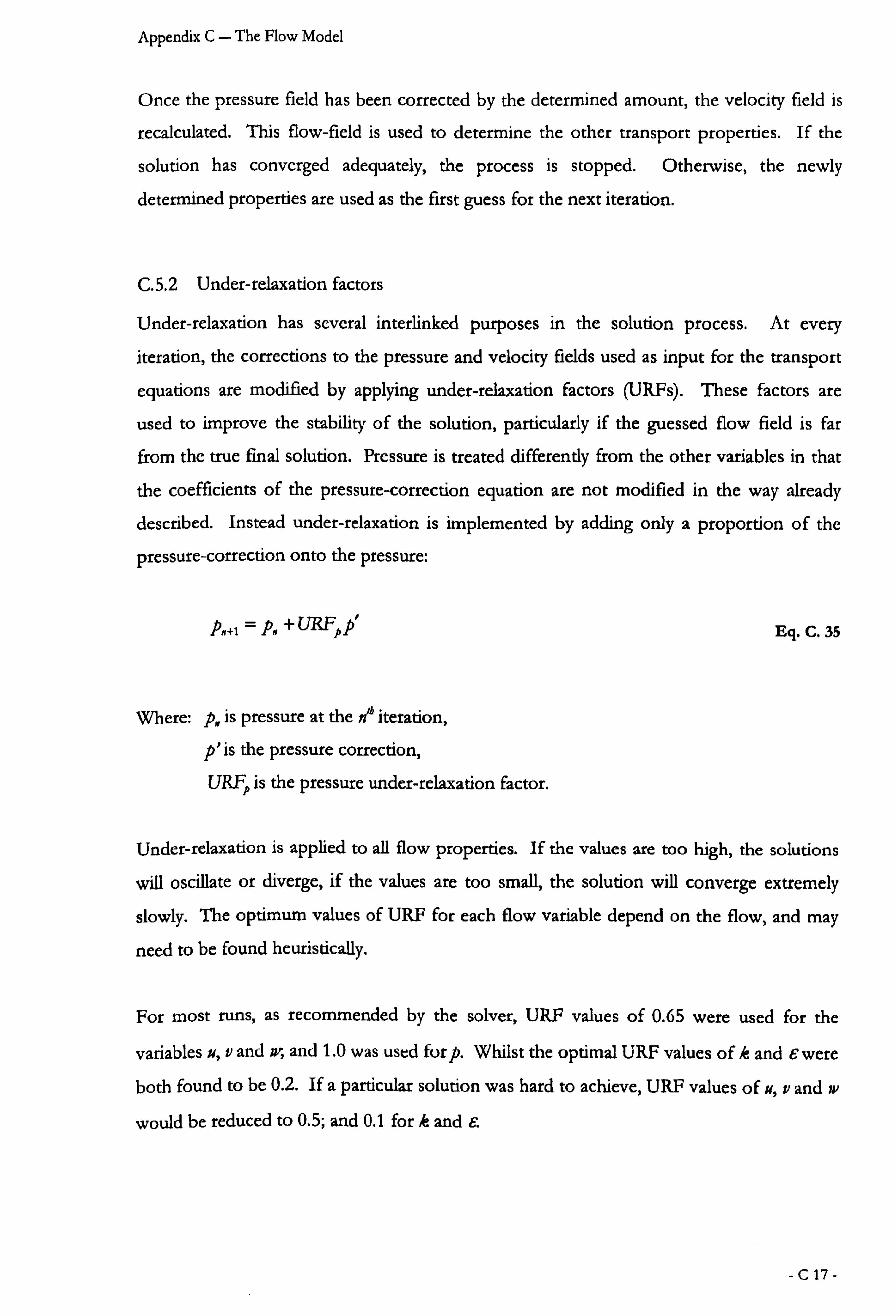
C. 5.2 Under-relaxation factors
Under-relaxation has several interlinked purposes in the solution process. At every
iteration, the corrections to the pressure and velocity fields used as input for the transport
equations are modified by applying under-relaxation factors (URFs). These factors are
used to improve the stability of the solution, particularly if the guessed flow field is far
from the true final solution. Pressure is treated differently from the other variables in that
the coefficients of the pressure-correction equation are not modified in the way already described. Instead under-relaxation is implemented by adding only a proportion of the
pressure-correction onto the pressure:
p. +, = pn + UKFF p' Eq. C. 35
Where: p� is pressure at the n'h iteration,
p' is the pressure correction, URFp is the pressure under-relaxation factor.
Under-relaxation is applied to all flow properties. If the values are too high, the solutions
will oscillate or diverge, if the values are too small, the solution will converge extremely
slowly. The optimum values of URF for each flow variable depend on the flow, and may
need to be found heuristically.
For most runs, as recommended by the solver, URF values of 0.65 were used for the
variables u, v and w, and 1.0 was used for p. Whilst the optimal URF values of k and e were
both found to be 0.2. If a particular solution was hard to achieve, URF values of u, v and w
would be reduced to 0.5; and 0.1 for k and C.
-C17-
Appendix D- Fortran Routines
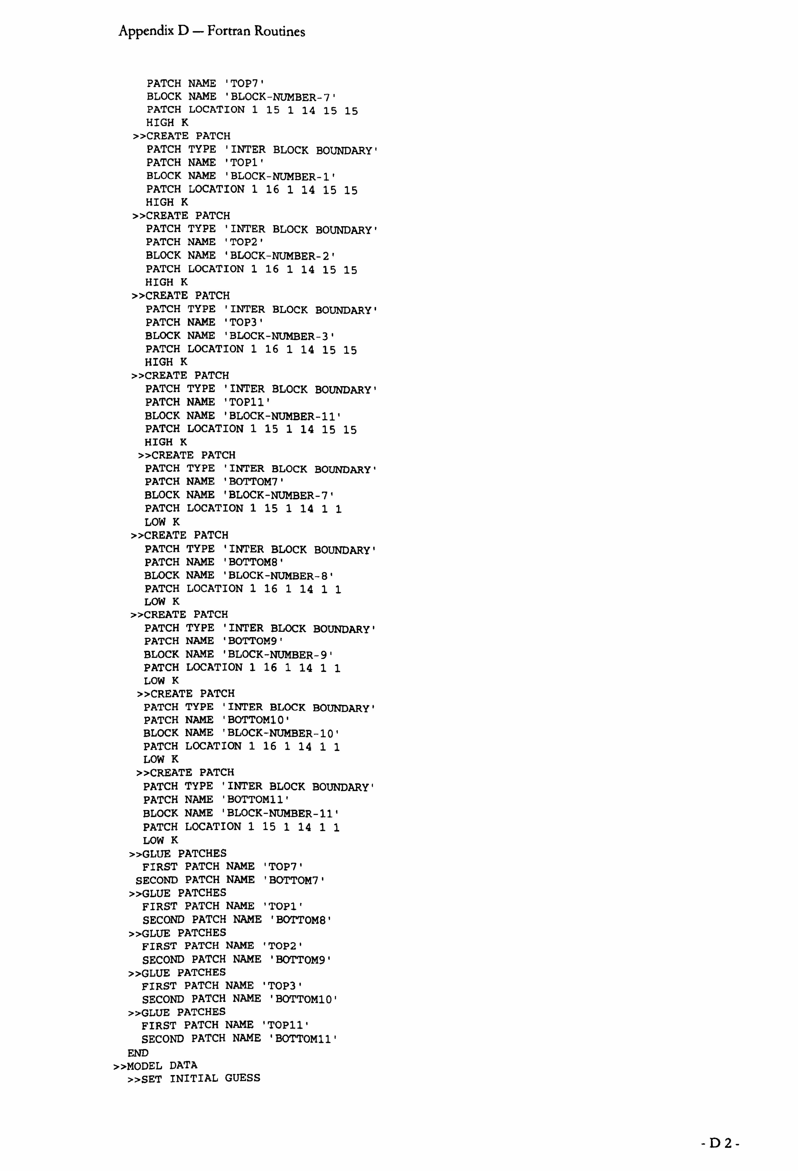
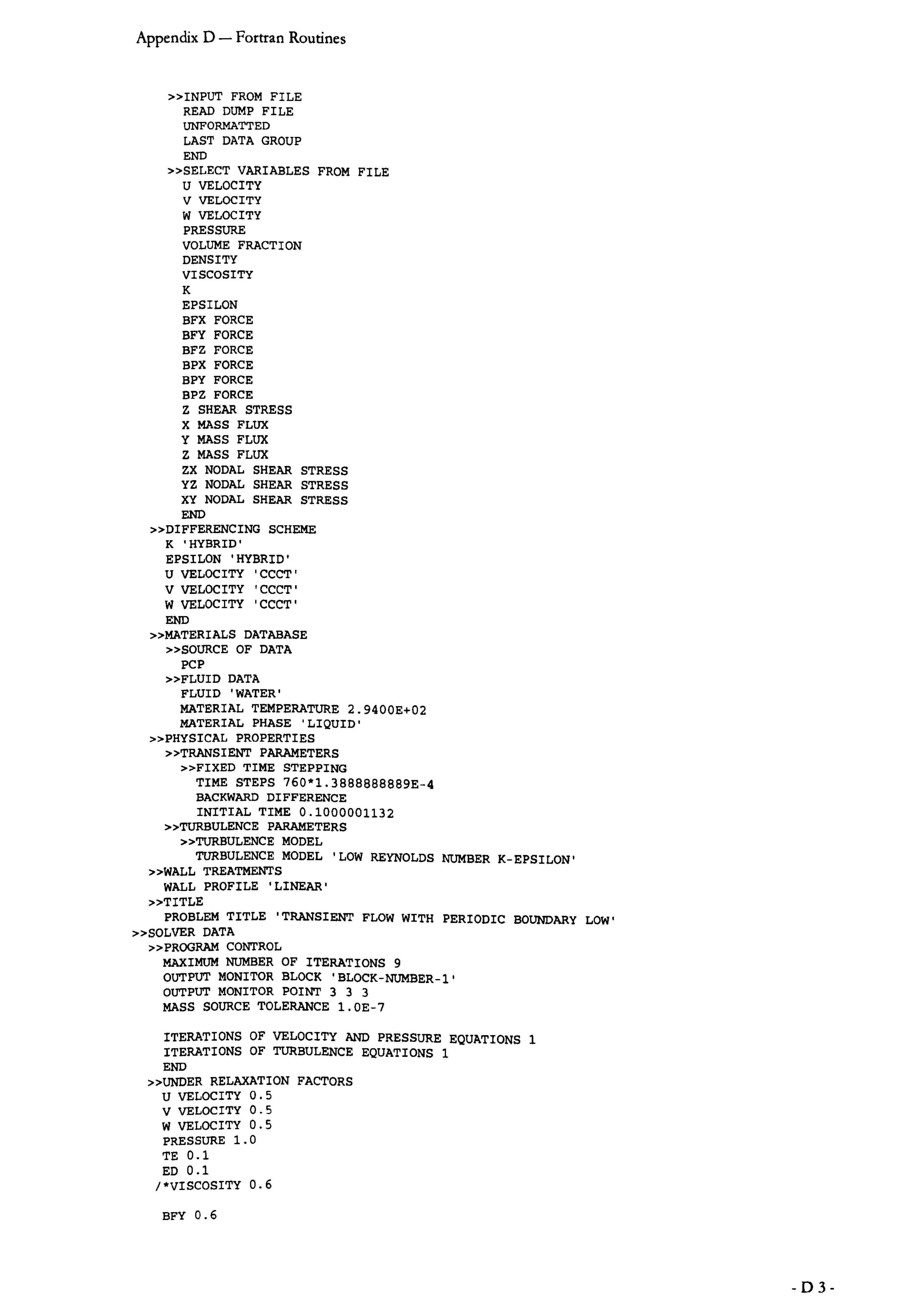
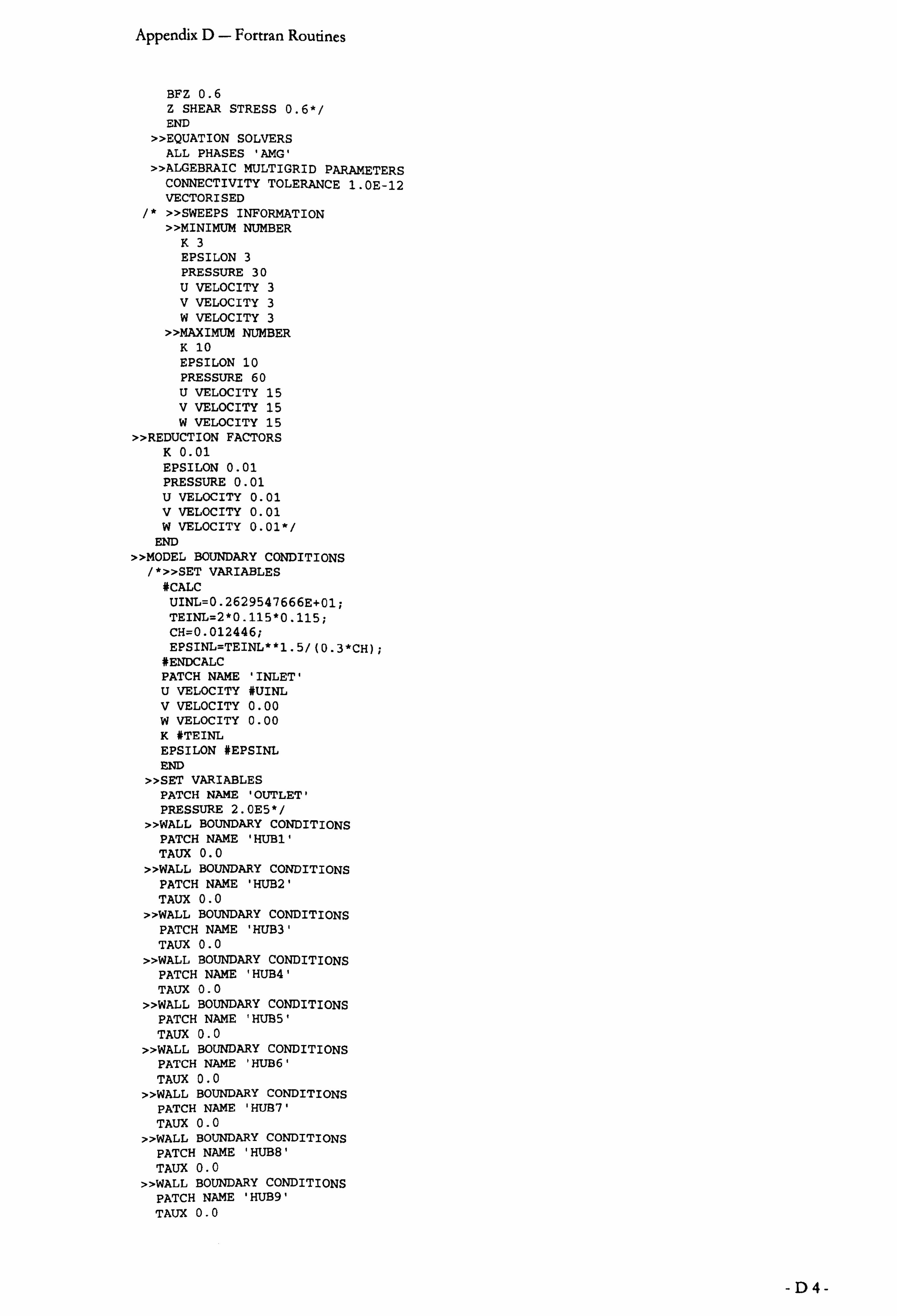
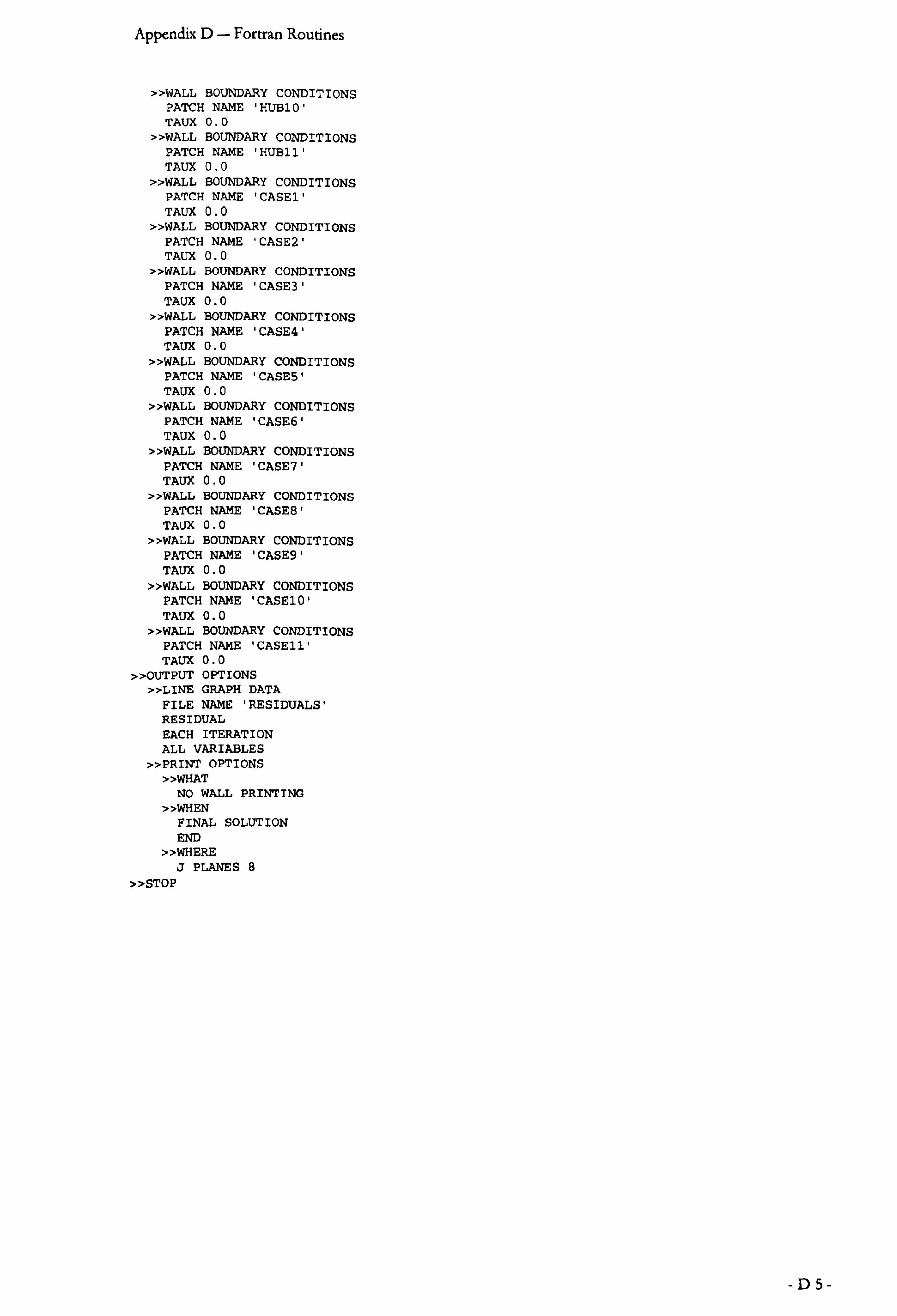
Appendix D Fortran Routines
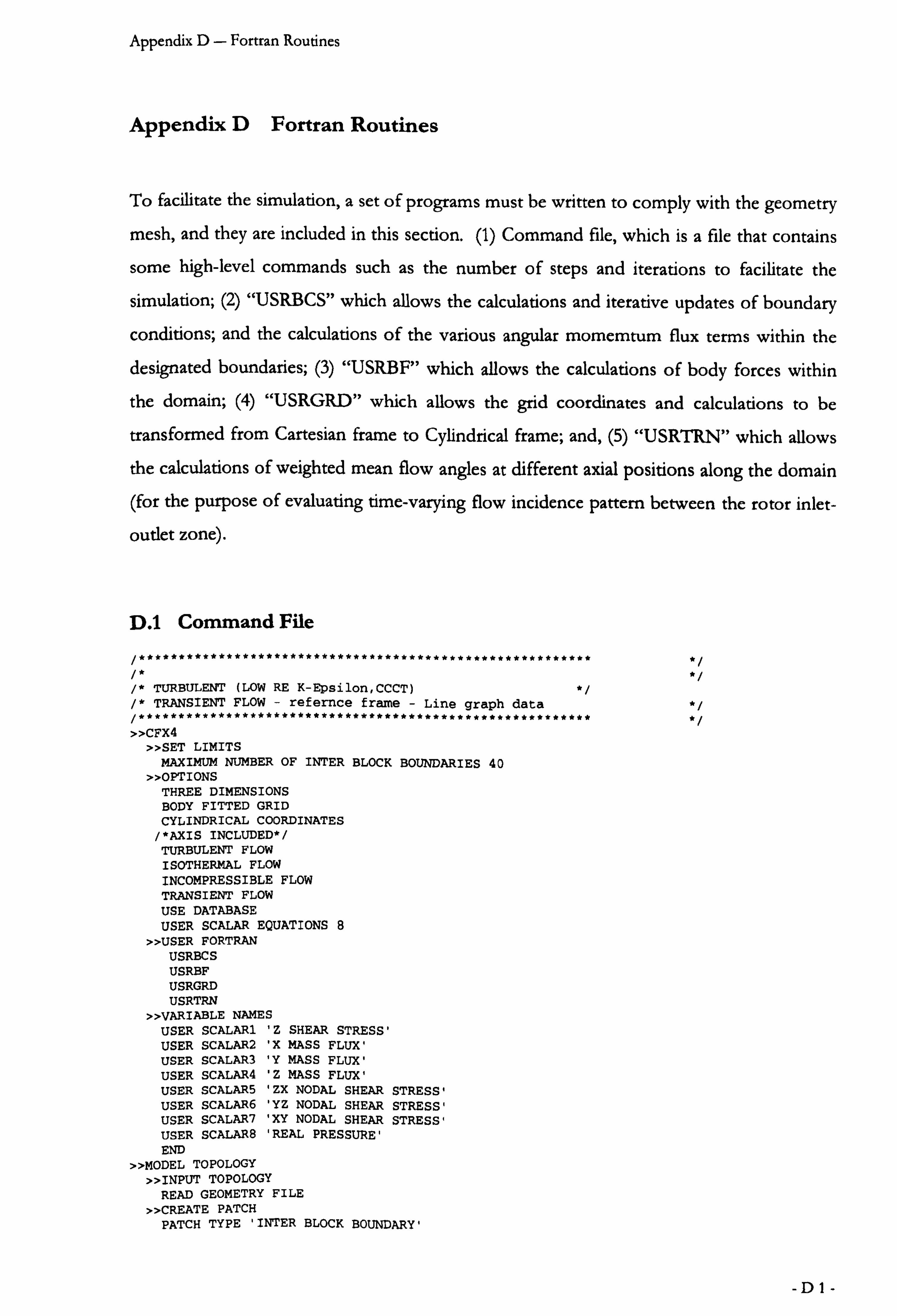
To facilitate the simulation, a set of programs must be written to comply with the geometry
mesh, and they are included in this section. (1) Command file, which is a file that contains
some high-level commands such as the number of steps and iterations to facilitate the
simulation; (2) "USRBCS" which allows the calculations and iterative updates of boundary
conditions; and the calculations of the various angular momemtum flux terms within the
designated boundaries; (3) "USRBF" which allows the calculations of body forces within
the domain; (4) "USRGRD" which allows the grid coordinates and calculations to be
transformed from Cartesian frame to Cylindrical frame; and, (5) "USRTRN" which allows
the calculations of weighted mean flow angles at different axial positions along the domain
(for the purpose of evaluating time-varying flow incidence pattern between the rotor inlet-
outlet zone).
D. 1 Command File
/* TURBULENT (LOW RE K-Epsilon, 000T) /* TRANSIENT FLOW - refernce frame - Line graph data
»CFX4 »SET LIMITS
MAXIMUM NUMBER OF INTER BLOCK BOUNDARIES 40 >>OPTIONS
THREE DIMENSIONS BODY FITTED GRID CYLINDRICAL COORDINATES
/*AXIS INCLUDED*/ TURBULENT FLOW ISOTHERMAL FLOW INCOMPRESSIBLE FLOW TRANSIENT FLOW USE DATABASE USER SCALAR EQUATIONS 8
>>USER FORTRAN USRBCS USRBF USRGRD USRTRN
»VARIABLE NAMES USER SCALAR1 Z SHEAR STRESS' USER SCALAR2 X MASS FLUX' USER SCALAR3 Y MASS FLUX' USER SCALAR4 Z MASS FLUX' USER SCALAR5 ZX NODAL SHEAR STRESS' USER SCALAR6 YZ NODAL SHEAR STRESS' USER SCALAR7 XY NODAL SHEAR STRESS' USER SCALARS REAL PRESSURE' END
»MODEL TOPOLOGY »INPUT TOPOLOGY
READ GEOMETRY FILE
>>CREATE PATCH PATCH TYPE 'INTER BLOCK BOUNDARY'
-DI-
Appendix D- Fortran Routines
PATCH NAME TOP7' BLOCK NAME 'BLOCK-NUMBER-7' PATCH LOCATION 1 15 1 14 15 15 HIGH K
>>CREATE PATCH
PATCH TYPE 'INTER BLOCK BOUNDARY PATCH NAME 'TOP1' BLOCK NAME BLOCK-NUMBER-1' PATCH LOCATION 1 16 1 14 15 15 HIGH K
>>CREATE PATCH PATCH TYPE 'INTER BLOCK BOUNDARY PATCH NAME TOP2'
BLOCK NAME BLOCK-NUMBER-2' PATCH LOCATION 1 16 1 14 15 15 HIGH K
>>CREATE PATCH PATCH TYPE 'INTER BLOCK BOUNDARY' PATCH NAME TOP3' BLOCK NAME BLOCK-NUMBER-3' PATCH LOCATION 1 16 1 14 15 15 HIGH K
>>CREATE PATCH PATCH TYPE 'INTER BLOCK BOUNDARY' PATCH NAME 'TOP11' BLOCK NAME 'BLOCK-NUMBER-11' PATCH LOCATION 1 15 1 14 15 15 HIGH K
>>CREATE PATCH PATCH TYPE 'INTER BLOCK BOUNDARY' PATCH NAME 'BOTTOM7'
BLOCK NAME 'BLOCK-NUMBER-7' PATCH LOCATION 1 15 1 14 11 LOW K
>>CREATE PATCH PATCH TYPE 'INTER BLOCK BOUNDARY' PATCH NAME 'BOTTOM8' BLOCK NAME 'BLOCK-NUMBER-8' PATCH LOCATION 1 16 1 14 11 LOW K
>CREATE PATCH PATCH TYPE 'INTER BLOCK BOUNDARY' PATCH NAME BOTTOM9'
BLOCK NAME 'BLOCK-NUMBER-9' PATCH LOCATION 1 16 1 14 11 LOW K
>>CREATE PATCH PATCH TYPE INTER BLOCK BOUNDARY' PATCH NAME BOTTOM10'
BLOCK NAME 'BLOCK-NUMBER-10' PATCH LOCATION 1 16 1 14 11 LOW K
> CREATE PATCH PATCH TYPE 'INTER BLOCK BOUNDARY' PATCH NAME 'BOTTOMII' BLOCK NAME 'BLOCK-NUMBER-11' PATCH LOCATION 1 15 1 14 11 LOW K
>>GLUE PATCHES FIRST PATCH NAME 'TOP7'
SECOND PATCH NAME 'BOTTOM7' > GLUE PATCHES
FIRST PATCH NAME 'TOP1' SECOND PATCH NAME 'BOTTOMS'
>>GLUE PATCHES FIRST PATCH NAME 'TOP2'
SECOND PATCH NAME 'BOTTOM9'
>>GLUE PATCHES
FIRST PATCH NAME 'TOP3' SECOND PATCH NAME 'BOTTOMIO'
> GLUE PATCHES FIRST PATCH NAME 'TOP11' SECOND PATCH NAME 'BOTTOMII'
END >MODEL DATA
»SET INITIAL GUESS
-D2-
Appendix D- Fortran Routines
»INPUT FROM FILE READ DUMP FILE UNFORMATTED LAST DATA GROUP
END
>>SELECT VARIABLES FROM FILE U VELOCITY V VELOCITY W VELOCITY PRESSURE VOLUME FRACTION DENSITY VISCOSITY K
EPSILON BFX FORCE BFY FORCE BFZ FORCE BPX FORCE BPY FORCE BPZ FORCE Z SHEAR STRESS X MASS FLUX Y MASS FLUX Z MASS FLUX ZX NODAL SHEAR STRESS YZ NODAL SHEAR STRESS XY NODAL SHEAR STRESS END
»DIFFERENCING SCHEME K 'HYBRID'
EPSILON 'HYBRID' U VELOCITY CCCT' V VELOCITY CCCT' W VELOCITY CCCT' END
»MATERIALS DATABASE >>SOURCE OF DATA
PCP >>FLUID DATA
FLUID 'WATER' MATERIAL TEMPERATURE 2.9400E+02 MATERIAL PHASE 'LIQUID'
>>PHYSICAL PROPERTIES
>>TRANSIENT PARAMETERS
>>FIXED TIME STEPPING
TIME STEPS 760*1.3888888889E-4 BACKWARD DIFFERENCE INITIAL TIME 0.1000001132
»TURBULENCE PARAMETERS >>TURBULENCE MODEL
TURBULENCE MODEL 'LOW REYNOLDS NUMBER K-EPSILON' »WALL TREATMENTS
WALL PROFILE 'LINEAR' »TITLE
PROBLEM TITLE 'TRANSIENT FLOW WITH PERIODIC BOUNDARY LOW' >>SOLVER DATA
>>PROGRAM CONTROL MAXIMUM NUMBER OF ITERATIONS 9 OUTPUT MONITOR BLOCK 'BLOCK-NUMBER-1' OUTPUT MONITOR POINT 333 MASS SOURCE TOLERANCE 1.0E-7
ITERATIONS OF VELOCITY AND PRESSURE EQUATIONS ITERATIONS OF TURBULENCE EQUATIONS 1 END
> UNDER RELAXATION FACTORS U VELOCITY 0.5 V VELOCITY 0.5 W VELOCITY 0.5 PRESSURE 1.0 TE 0.1 ED 0.1
/*VISCOSITY 0.6
BFY 0.6
-D3-
Appendix D- Fortran Routines
BFZ 0.6 Z SHEAR STRESS 0.6*/ END
>>EQUATION SOLVERS ALL PHASES 'AMG'
>>ALGEBRAIC MULTIGRID PARAMETERS CONNECTIVITY TOLERANCE 1.0E-12 VECTORISED
/* >>SWEEPS INFORMATION »MINIMUM NUMBER
K3 EPSILON 3
PRESSURE 30 U VELOCITY 3 V VELOCITY 3 W VELOCITY 3
»MAXIMUM NUMBER K 10 EPSILON 10 PRESSURE 60 U VELOCITY 15 V VELOCITY 15 W VELOCITY 15
>>REDUCTION FACTORS K 0.01 EPSILON 0.01 PRESSURE 0.01 U VELOCITY 0.01 V VELOCITY 0.01 W VELOCITY 0.01*/
END »MODEL BOUNDARY CONDITIONS
/*»SET VARIABLES #CALC
UINL=0.2629547666E+01; TEINL=2*0.115*0.115; CH=0.012446; EPSINL=TEINL**1.5/(0.3*CH);
#ENDCALC PATCH NAME INLET' U VELOCITY #UINL V VELOCITY 0.00 W VELOCITY 0.00 K #TEINL EPSILON #EPSINL END
»SET VARIABLES PATCH NAME OUTLET' PRESSURE 2.0E5*/
»WALL BOUNDARY CONDITIONS PATCH NAME 'HUB1' TAUX 0.0
»WALL BOUNDARY CONDITIONS PATCH NAME HUB2' TAUX 0.0
»WALL BOUNDARY CONDITIONS PATCH NAME HUBS' TAUX 0.0
»WALL BOUNDARY CONDITIONS PATCH NAME HUB4' TAUX 0.0
»WALL BOUNDARY CONDITIONS PATCH NAME 'HUBS' TAUX 0.0
»WALL BOUNDARY CONDITIONS PATCH NAME HUB6' TAUX 0.0
»WALL BOUNDARY CONDITIONS PATCH NAME HUB7' TAUE 0.0
»WALL BOUNDARY CONDITIONS
PATCH NAME HUBS'
TAUX 0.0
»WALL BOUNDARY CONDITIONS PATCH NAME HUB9' TAUX 0.0
-D4-
Appendix D- Fortran Routines
»WALL BOUNDARY CONDITIONS PATCH NAME 'HUB10' TAUX 0.0
»WALL BOUNDARY CONDITIONS PATCH NAME 'HUB11'
TAUX 0.0 »WALL BOUNDARY CONDITIONS
PATCH NAME 'CASEl'
TAUX 0.0 »WALL BOUNDARY CONDITIONS
PATCH NAME CASE2' TAUX 0.0
»WALL BOUNDARY CONDITIONS PATCH NAME CASE3'
TAUX 0.0 »WALL BOUNDARY CONDITIONS
PATCH NAME CASE4' TAUX 0.0
»WALL BOUNDARY CONDITIONS PATCH NAME 'CASE5'
TAUX 0.0 »WALL BOUNDARY CONDITIONS
PATCH NAME CASE6' TAUX 0.0
»WALL BOUNDARY CONDITIONS PATCH NAME CASE7' TAUX 0.0
»WALL BOUNDARY CONDITIONS PATCH NAME 'CASE8' TAUX 0.0
»WALL BOUNDARY CONDITIONS PATCH NAME 'CASE9' TAUX 0.0
»WALL BOUNDARY CONDITIONS PATCH NAME 'CASE10' TAUE 0.0
»WALL BOUNDARY CONDITIONS PATCH NAME 'CASE11' TAUE 0.0
»OUTPUT OPTIONS >>LINE GRAPH DATA
FILE NAME 'RESIDUALS' RESIDUAL
EACH ITERATION ALL VARIABLES
>>PRINT OPTIONS >>WHAT
NO WALL PRINTING
>>WHEN FINAL SOLUTION END
>>WHERE J PLANES 8
»STOP
-D5-
Appendix D- Fortran Routines
D. 2 USRBCS
SUBROUTINE USRBCS(VARBCS, VARAMB, A, B, C, ACND, BCND, CCND + IWGVEL, NDVWAL + , FLOUT, NLABEL, NSTART, NEND, NCST, NCEN
+ , U, V, W, P, VFRAC, DEN, VIS, TE, ED, RS, T, H, RF, SCAL
+ , XP, YP, ZP, VOL, AREA, VPOR, ARPOR, WFACT, IPT
+ , IBLK, IPVERT, IPNODN, IPFACN, IPNODF, IPNODB, IPFACB
+ , WORK, IWORK, CWORK)
C
C C USER ROUTINE TO SET REALS AT BOUNDARIES.
C
C »> IMPORTANT <<< C »> <<< C »> USERS MAY ONLY ADD OR ALTER PARTS OF THE SUBROUTINE WITHIN <<< C »> THE DESIGNATED USER AREAS <<< C C*********************************************************************** C C THIS SUBROUTINE IS CALLED BY THE FOLLOWING SUBROUTINE C CUSR SRLIST C C*********************************************************************** C CREATED C 30/11/88 ADB C MODIFIED C 08/09/90 ADB RESTRUCTURED FOR USER-FRIENDLINESS. C 10/08/91 IRH FURTHER RESTRUCTURING ADD ACND BCND CCND C 22/09/91 IRH CHANGE ICALL TO IUCALL + ADD /SPARM/ C 10/03/92 PHA UPDATE CALLED BY COMMENT, ADD RF ARGUMENT, C CHANGE LAST DIMENSION OF RS TO 6 AND IVERS TO 2 C 03/06/92 PHA ADD PRECISION FLAG AND CHANGE IVERS TO 3 C 30/06/92 NSW INCLUDE FLAG FOR CALLING BY ITERATION C INSERT EXTRA COMMENTS C 03/08/92 NSW MODIFY DIMENSION STATEMENTS FOR VAX C 21/12/92 CSH INCREASE IVERS TO 4 C 02/08/93 NSW INCORRECT AND MISLEADING COMMENT REMOVED C 05/11/93 NSW INDICATE USE OF FLOUT IN MULTIPHASE FLOWS
C 23/11/93 CSH EXPLICITLY DIMENSION IPVERT ETC. C 01/02/94 NSW SET VARIABLE POINTERS IN WALL EXAMPLE. C CHANGE FLOW3D TO CFDS-FLOW3D. C MODIFY MULTIPHASE MASS FLOW BOUNDARY TREATMENT.
C 03/03/94 FHW CORRECTION OF SPELLING MISTAKE
C 02/07/94 BAS SLIDING GRIDS - ADD NEW ARGUMENT IWGVEL C TO ALLOW VARIANTS OF TRANSIENT-GRID WALL BC C CHANGE VERSION NUMBER TO 5 C 09/08/94 NSW CORRECT SPELLING C MOVE 'IF(IUSED. EQ. 0) RETURN' OUT OF USER AREA C 19/12/94 NSW CHANGE FOR CFX-F3D C 02/02/95 NSW CHANGE COMMON /IMFBMP/ C 02/06/97 NSW MAKE EXAMPLE MORE LOGICAL C 02/07/97 NSW UPDATE FOR CFX-4 C C++. **. +rar*****************, t******«*********rr***********w*ºw*«******k"
C C SUBROUTINE ARGUMENTS
C
C VARBCS - REAL BOUNDARY CONDITIONS C VARAMB - AMBIENT VALUE OF VARIABLES CA- COEFFICIENT IN WALL BOUNDARY CONDITION CB- COEFFICIENT IN WALL BOUNDARY CONDITION CC- COEFFICIENT IN WALL BOUNDARY CONDITION C ACND - COEFFICIENT IN CONDUCTING WALL BOUNDARY CONDITION C BCND - COEFFICIENT IN CONDUCTING WALL BOUNDARY CONDITION C CCND - COEFFICIENT IN CONDUCTING WALL BOUNDARY CONDITION C IWGVEL - USAGE OF INPUT VELOCITIES (0 = AS IS, 1 = ADD GRID MOTION) C NDVWAL - FIRST DIMENSION OF ARRAY IWGVEL C FLOUT - MASS FLOW/FRACTIONAL MASS FLOW C NLABEL - NUMBER OF DISTINCT OUTLETS C NSTART - ARRAY POINTER
C NEND - ARRAY POINTER
-D6-
Appendix D- Fortran Routines
C NCST - ARRAY POINTER C NCEN - ARRAY POINTER CU-U COMPONENT OF VELOCITY
CV-V COMPONENT OF VELOCITY
CW-W COMPONENT OF VELOCITY
CP- PRESSURE
C VFRAC - VOLUME FRACTION C DEN - DENSITY OF FLUID C VIS - VISCOSITY OF FLUID C TE - TURBULENT KINETIC ENERGY C ED - EPSILON C RS - REYNOLD STRESSES
CT- TEMPERATURE
CH- ENTHALPY C RF - REYNOLD FLUXES
C SCAL - SCALARS (THE FIRST 'NCONC' OF THESE ARE MASS FRACTIONS)
C XP -X COORDINATES OF CELL CENTRES C YP -Y COORDINATES OF CELL CENTRES C ZP -Z COORDINATES OF CELL CENTRES C VOL - VOLUME OF CELLS C AREA - AREA OF CELLS C VPOR - POROUS VOLUME
C ARPOR - POROUS AREA C WFACT - WEIGHT FACTORS C C IPT - 1D POINTER ARRAY C IBLK - BLOCK SIZE INFORMATION
C IPVERT - POINTER FROM CELL CENTERS TO 8 NEIGHBOURING VERTICES
C IPNODN - POINTER FROM CELL CENTERS TO 6 NEIGHBOURING CELLS C IPFACN - POINTER FROM CELL CENTERS TO 6 NEIGHBOURING FACES
C IPNODF - POINTER FROM CELL FACES TO 2 NEIGHBOURING CELL CENTERS
C IPNODB - POINTER FROM BOUNDARY CENTERS TO CELL CENTERS
C IPFACB - POINTER TO NODES FROM BOUNDARY FACES
C C WORK - REAL WORKSPACE ARRAY
C IWORK - INTEGER WORKSPACE ARRAY
C CWORK - CHARACTER WORKSPACE ARRAY C C SUBROUTINE ARGUMENTS PRECEDED WITH A '*' ARE ARGUMENTS THAT MUST
C BE SET BY THE USER IN THIS ROUTINE. C C NOTE THAT OTHER DATA MAY BE OBTAINED FROM CFX-4 USING THE
C ROUTINE GETADD, FOR FURTHER DETAILS SEE THE VERSION 4
C USER MANUAL. C
LOGICAL LDEN, LVIS, LTURB, LTEMP, LBUOY, LSCAL, LCOMP
+ , LRECT, LCYN, LAXIS, LPOROS, LTRANS
C CHARACTER*(*) CWORK
C C+++++++++++++++++ USER AREA 1+++++++++++++++++++++++++++++++++++++++++
C---- AREA FOR USERS EXPLICITLY DECLARED VARIABLES
C REAL TSUM, INERTIA, ACCE, AREAM, WOLD, WTEMP, WNEW, UOLD, UNEW, WABS,
+ WVSUM, VSUM, DELTAR, TNET,
+ AMP, FREQ, PERIOD, OMEGA, REMAIN, PHASE, RADIAN, PULSE,
+ MOINA, MOINB, MOINC, MOIND, MOOUTA, MOOUTB, MOOUTC, MOOUTD,
+ FIAOLD, FIANEW, FIBOLD, FIBNEW, FIAOLDP, FIANEWP, FIBOLDP, FIBNEWP,
+ TROTOR, TFIA, TFIB, TFIAP, TFIBP, TFRIC, MASSIA, MASSIC, MASSO,
+ THETAXO, RTHETAO, XRO, XTHETAO, + THETAXJ, RTHETAJ, XRJ, XTHETAJ,
+ THETAXD, RTHETAD, XRD, XTHETAD,
+ THETAXP, RTHETAP, XRP, XTHETAP, UA
INTEGER ITXT, ISEQF, BLADEN, DOMAINN, IUSRITER, IUSRSTEP
C C+++++++++++++++++ END OF USER AREA 1++++++++++++++++++++++++++++++++++
C COMMON
+ /ALL/ NBLOCK, NCELL, NBDRY, NNODE, NFACE, NVERT, NDIM
+ /ALLWRK/ NRWS, NIWS, NCWS, IWRFRE, IWIFRE, IWCFRE
+ /ADDIMS/ NPHASE, NSCAL, NVAR, NPROP
+ , NDVAR, NDPROP, NDXNN, NDGEOM, NDCOEF, NILIST, NRLIST, NTOPOL
+ /BCSOUT/ IFLOUT
+ /CHKUSR/ IVERS, IUCALL, IUSED
+ /DEVICE/ NREAD, NWRITE, NRDISK, NWDISK
-D7-
Appendix D- Fortran Routines
/IDUM/ ILEN, JLEN /IMFBMP/ IMFBMP, JMFBMP /LOGIC/ LDEN, LVIS, LTURB, LTEMP, LBUOY, LSCAL, LCOMP
, LRECT, LCYN, LAXIS, LPOROS, LTRANS
/MLTGRD/ MLEVEL, NLEVEL, ILEVEL
/SGLDBL/ IFLGPR, ICHKPR /SPARM/ SMALL, SORMAX, NITER, INDPRI, MAXIT, NODREF, NODMON
/TRANSI/ NSTEP, KSTEP, MF, INCORE
/TIMUSR/ DTUSR /TRANSR/ TIME, DT, DTINVF, TPARM /UBCSFL/ IUBCSF
C C+++++++++++++++++ USER AREA 2+++++++++++++++++++++++++++++++++++++++++
C---- AREA FOR USERS TO DECLARE THEIR OWN COMMON BLOCKS
C THESE SHOULD START WITH THE CHARACTERS 'UC' TO ENSURE C NO CONFLICT WITH NON-USER COMMON BLOCKS
COMMON + /UC1/ TSUM, INERTIA, ACCE, AREAM, WOLD, WTEMP, WNEW, UOLD, UNEW, WABS,
+ WVSUM, VSUM, DELTAR, TNET, + AMP, FREQ, PERIOD, OMEGA, REMAIN, PHASE, RADIAN, PULSE,
+ MOINA, MOINB, MOINC, MOIND, MOOUTA, MOOUTB, MOOUTC, MOOUTD, + FIAOLD, FIANEW, FIBOLD, FIBNEW, FIAOLDP, FIANEWP, FIBOLDP, FIBNEWP,
+ TROTOR, TFIA, TFIB, TFIAP, TFIBP, TFRIC, MASSIA, MASSIC, MASSO,
+ THETAXO, RTHETAO, XRO, XTHETAO, + THETAXJ, RTHETAJ, XRJ, XTHETAJ,
+ THETAXD, RTHETAD, XRD, XTHETAD, + THETAXP, RTHETAP, XRP, XTHETAP, UA
C C+++++++++++++++++ END OF USER AREA 2++++++++++++++++++++++++++++++++++ C
DIMENSION + VARBCS(NVAR, NPHASE, NCELL+I: NNODE), VARAMB(NVAR, NPHASE)
+, A(4+NSCAL, NPHASE, NSTART: *)
+, B(4+NSCAL, NPHASE, NSTART: *), C(4+NSCAL, NPHASE, NSTART: *)
+, FLOUT(*), ACND(NCST: *), BCND(NCST: *), CCND(NCST: *)
+, IWGVEL(NDVWAL, NPHASE)
DIMENSION
+ U(NNODE, NPHASE), V(NNODE, NPHASE), W(NNODE, NPHASE), P(NNODE, NPHASE)
+, VFRAC(NNODE, NPHASE), DEN(NNODE, NPHASE), VIS(NNODE, NPHASE)
+, TE(NNODE, NPHASE), ED(NNODE, NPHASE), RS(NNODE, NPHASE, 6)
+, T(NNODE, NPHASE), H(NNODE, NPHASE), RF(NNODE, NPHASE, 4)
+, SCAL(NNODE, NPHASE, NSCAL)
DIMENSION
+ XP(NNODE), YP(NNODE), ZP(NNODE)
+, VOL(NCELL), AREA(NFACE, 3), VPOR(NCELL), ARPOR(NFACE, 3), WFACT(NFACE)
+, IPT(*), IBLK(5, NBLOCK)
+, IPVERT(NCELL, 8), IPNODN(NCELL, 6), IPFACN(NCELL, 6), IPNODF(NFACE, 4)
+, IPNODB(NBDRY, 4), IPFACB(NBDRY)
+, IWORK(*), WORK(*), CWORK(*) C C+++++++++++++++++ USER AREA 3+++++++++++++++++++++++++++++++++++++++++
C____ AREA FOR USERS TO DIMENSION THEIR ARRAYS
C CHARACTER *15 USRBLADE, USRDOM DIMENSION USRBLADE(0: 50), USRDOM(0: 11) REAL USRPRESS(10,20,30), USRMEAN(20),
+ USRRAD(20,30) C---- AREA FOR USERS TO DEFINE DATA STATEMENTS
C C+++++++++++++++++ END OF USER AREA 3++++++++++++++++++++++++++++++++++
C C---- STATEMENT FUNCTION FOR ADDRESSING
IP(I, J, K)=IPT((K-1)*ILEN*JLEN+(J-1)*ILEN+I) C C__--VERSION NUMBER OF USER ROUTINE AND PRECISION FLAG
C IVERS=5 ICHKPR =1
C C+++++++++++++++++ USER AREA 4+++++++++++++++++++++++++++++++++++++++++
C---- TO USE THIS USER ROUTINE FIRST SET IUSED=l IUSED=1
C AND SET IUBCSF FLAG:
C BOUNDARY CONDITIONS NOT CHANGING
-D8-
Appendix D- Fortran Routines
C IUBCSF=0 C BOUNDARY CONDITIONS CHANGING WITH ITERATION C IUBCSF=1
C BOUNDARY CONDITIONS CHANGING WITH TIME C IUBCSF=2 C BOUNDARY CONDITIONS CHANGING WITH TIME AND ITERATION
IUBCSF=3 C+++++++++++++++++ END OF USER AREA 4++++++++++++++++++++++++++++++++++ C
IF (IUSED. EQ. O) RETURN C C---- FRONTEND CHECKING OF USER ROUTINE
IF (IUCALL. EQ. O) RETURN C C+++++++++++++++++ USER AREA 5+++++++++++++++++++++++++++++++++++++++++
IPHASE=1 C C IF (KSTEP. EQ. 0) THEN C ISEQF=O C CALL FILCON('USRBCS', 'tsum. txt', 'OPEN', 'FORMATTED', C+ 'NEW', ITXT, ISEQF, IOST, IERR) C C IF (IERR. NE. O) THEN
C CALL FILERR('USRBCS', 'tsum. txt', 'OPEN', 'NEW', C+ ITXT, ISEQF, IOST, IERR) C END IF C ENDIF C C----INITIAL CONDITIONS FOR RESTART C
IUSRITER=9 IUSRSTEP=760
C IF (NITER. LE. 1) THEN
C IF (KSTEP. EQ. 0) THEN
UNEW=0.2629547596E+01 WNEW=-0.3998958130E+03 WOLD=-0.3998956604E+03
FIAOLD=-1.754262513E-07 FIANEW=-1.754303014E-07 FIBOLD=1.516304837E-05 FIBNEW=1.516306384E-05 FIAOLDP=-1.020277622E-07 FIANEWP=-1.020272293E-07 FIBOLDP=3.917623417E-06 FIBNEWP=3.917619324E-06
DT=0.0005 UOLD=UNEW
AMP=0.4198 FREQ=20
PERIOD=1/FREQ OMEGA=2*3.14159265359/PERIOD
ELSE C C---- SET WOLD EQUALS TO THE ANGULAR VELOCITY AT THE TIME STEP C
WOLD=WNEW FIAOLD=FIANEW FIBOLD=FIBNEW FIAOLDP=FIANEWP FIBOLDP=FIBNEWP ENDIF
ENDIF C C---- TO FIND THE ANGULAR ACCELERATION OF THE BLADE AT EACH TIME STEP C
AREAM=0.0 TSUM=0.0 TNET=0.0 WABS=0.0 WVSUM=0.0
VSUM=0.0 MOINA=0.0 MOINB=0.0
-D9-
Appendix D- Fortran Routines
MOINC=0.0 MOIND=0.0 MOOUTA=0.0 MOOUTB=0.0 MOOUTC=0.0 MOOUTD=0.0
MASSIA=0.0 MASSIC=0.0 MASSO=0.0 THETAXO=0.0 RTHETAO=0.0
XRO=0.0 XTHETAO=0.0 THETAXJ=0.0 RTHETAJ=0.0
XRJ=0.0 XTHETAJ=0.0 THETAXD=0.0 RTHETAD=0.0
XRD=0.0 XTHETAD=0.0 THETAXP=0.0 RTHETAP=0.0
XRP=0.0 XTHETAP=0.0
IF (NITER. EQ. IUSRITER) THEN FIANEW=0.0 FIBNEW=0.0 FIANEWP=0.0 FIBNEWP=0.0
ENDIF
INERTIA=3.24885667E-09 C C C---- SET BLADEN TO BE BLADE1 TO BLADE6
USRBLADE(1)='BLADEI' USRBLADE(2)='BLADE2' USRBLADE(3)='BLADE3' USRBLADE(4)='BLADE4' USRBLADE(5)='BLADE5' USRBLADE(6)='BLADE6'
C DO 134 BLADEN=1,6
CALL IPREC(USRBLADE(BLADEN), 'PATCH', 'CENTRES', IPT, + ILEN, JLEN, KLEN, CWORK, IWORK)
C C---- GET SCALAR NUMBER CORRESPONDING TO THETA(Z) SHEAR STRESS C
CALL GETSCA ('Z SHEAR STRESS', ICS1, CWORK) C C---- LOOP OVER ALL WALL CELL CENTRES LOCATION IN WALLS C C234567891123456759212345678931234567894123456789512345678961233456789712 C LOOP OVER PATCH C
DO 133 K=1, KLEN DO 132 J=1, JLEN
DO 131 I=1, ILEN C C USE STATEMENT FUNCTION IP TO GET ADDRESSES
INODE=IP(I, J, K) IBDRY=INODE-NCELL IFACE=IPFACB(IBDRY) AREAM=SQRT(AREA(IFACE, 1)**2+
+ AREA(IFACE, 2)**2+
+ AREA(IFACE, 3)**2)
C TSUM=TSUM-P(INODE, 1)*YP(INODE)*AREA(IFACE, 3)-
+ YP(INODE)*SCAL(INODE, 1, ICS1)*AREAM C
IF ((NITER. EQ. IUSRITER). AND. (KSTEP. EQ. IUSRSTEP)) THEN WRITE(ITXT, 900)I, J, K, P(INODE, 1), SCAL(INODE, 1, ICS1), XP(INODE),
+ YP(INODE), ZP(INODE), AREA(IFACE, 1), AREA(IFACE, 2), AREA(IFACE, 3), + AREAM, TSUM
900 FORMAT(I5, I5, I5,10(2X, E17.10)) ENDIF
-D10-
Appendix D- Fortran Routines
C 131 CONTINUE 132 CONTINUE 133 CONTINUE 134 CONTINUE
C C C
IF (KSTEP. EQ. 0) THEN
ACCE=-3.349977136E-01 ELSE
TFRIC=0.0 TNET=TSUM+TFRIC
ACCE=TNET/INERTIA
ENDIF
C C C---- TO UPDATE THE INLET FLOW VELOCITY USING 1ST ORDER C---- BACKWARD DIFFERENCING C C---- OPEN THE FILE CONTAINING DATA ABOUT ANGULAR VELOCITY(WNEW) C234567891123456789212345678931234567894123456789512345678961233456789712
IF (KSTEP. EQ. O) THEN ISEQF=O
CALL FILCON('USRBCS', 'angular. txt',, OPEN', 'FORMATTED', + 'NEW', ITXT, ISEQF, IOST, IERR)
C IF (IERR. NE. O) THEN CALL FILERR('USRBCS', 'angular. txt', 'OPEN', 'NEW',
+ ITXT, ISEQF, IOST, IERR) END IF
ENDIF C C C
IF (KSTEP. EQ. 40) THEN REMAIN=TIME/PERIOD-INT(TIME/PERIOD) PHASE=PERIOD*REMAIN ENDIF
C IF ((NITER. EQ. 1). AND. (KSTEP. GE. 41)) THEN
RADIAN=OMEGA*(TIME-PHASE) PULSE=AMP*SIN(RADIAN)
UNEW=UOLD*(1+PULSE) ENDIF
C C---- SET WNEW TO THE VELOCITY AT THE NEXT TIME STEP C
WNEW = WOLD+ACCE*DT C
IF (KSTEP. GE. 1) THEN CALL GETSCA ('X MASS FLUX', ICS2, CWORK) CALL GETSCA ('Y MASS FLUX', ICS3, CWORK) CALL GETSCA ('Z MASS FLUX', ICS4, CWORK) CALL GETSCA ('ZX NODAL SHEAR STRESS', ICS5, CWORK) CALL GETSCA ('YZ NODAL SHEAR STRESS', ICS6, CWORK) CALL GETSCA ('XY NODAL SHEAR STRESS', ICS7, CWORK) ENDIF
C C234567891123456789212345678931234567894123456789512345678961233456789712
CALL IPREC('INLET', 'PATCH', 'CENTRES', IPT, + ILEN, JLEN, KLEN, CWORK, IWORK)
C INTERROGATE GETVAR FOR VARIABLE NUMBERS C
CALL GETVAR('USRBCS', 'W ', IW) CALL GETVAR('USRBCS', 'U ', IU)
C
C LOOP OVER PATCH DO 103 K=1, KLEN
DO 102 J=1, JLEN DO 101 I=1, ILEN
C C USE STATEMENT FUNCTION IP TO GET ADDRESSES
INODE=IP(I, J, K) C C SET VARBCS
-D11-
Appendix D- Fortran Routines
VARBCS(IW, IPHASE, INODE) _ -YP(INODE)*WNEW IF (KSTEP. LE. 40) THEN
VARBCS(IU, IPHASE, INODE) = 0.2629547596E+01 ELSE
VARBCS(IU, IPHASE, INODE) = UNEW ENDIF
c c
IF (NITER. EQ. IUSRITER) THEN IBDRY=INODE-NCELL
IFACE=IPFACB(IBDRY) WABS = W(INODE, 1)+YP(INODE)*WNEW
C234567891123456789212345678931234567894123456789512345678961233456789712 MOINA =MOINA+DEN(INODE, 1)*YP(INODE)*U(INODE, 1)*WABS*AREA(IFACE, 1) MOINB =MOINB+DEN(INODE, 1)*YP(INODE)*U(INODE, 1)*W(INODE, 1)
+ *AREA(IFACE, 1) C
MASSIA=MASSIA+SCAL(INODE, 1, ICS2)*AREA(IFACE, 1)+SCAL(INODE, 1, ICS3) + *AREA(IFACE, 2)+SCAL(INODE, 1, ICS4)*AREA(IFACE, 3)
C IF (KSTEP. EQ. IUSRSTEP) THEN
WRITE(ITXT, 901)I, J, K, P(INODE, 1), VOL(INODE), WNEW, WABS, U(INODE, 1), + V(INODE, 1), W(INODE, 1), YP(INODE), + AREA(IFACE, 1), AREA(IFACE, 2), AREA(IFACE, 3)
901 FORMAT(I5, I5, I5,11(2X, E17.10)) ENDIF
C ENDIF
101 CONTINUE
102 CONTINUE
103 CONTINUE
C
C C---- TO LOCATE JUST UPSTREAM FINDING ANG. MOMENTUM C
IF (NITER. EQ. IUSRITER) THEN CALL IPREC('BLOCK-NUMBER-7', 'BLOCK', 'CENTRES', IPT,
+ ILEN, JLEN, KLEN, CWORK, IWORK) C INTERROGATE GETVAR FOR VARIABLE NUMBERS C C LOOP OVER PATCH
I=14 DO 161 J=1, JLEN
DO 162 K=1, KLEN C C USE STATEMENT FUNCTION IP TO GET ADDRESSES
INODE=IP(I, J, K) WAGS = W(INODE, 1)+YP(INODE)*WNEW UA=U(INODE, 1)*AREA(INODE, 1)+V(INODE, 1)*AREA(INODE, 2)+
+ W(INODE, 1)*AREA(INODE, 3) c C234567891123456789212345678931234567894123456789512345678961233456789712
MOINC =MOINC+DEN(INODE, 1)*YP(INODE)*WABS*UA MOIND =MOIND+DEN(INODE, 1)*YP(INODE)*W(INODE, 1)*UA
C MASSIC=MASSIC+SCAL(INODE, 1, ICS2)*AREA(INODE, 1)+SCAL(INODE, 1, ICS3)
+ *AREA(INODE, 2)+SCAL(INODE, 1, ICS4)*AREA(INODE, 3) C
IF (KSTEP. EQ. IUSRSTEP) THEN C234567891123456789212345678931234567894123456789512345678961233456789712
WRITE(ITXT, 902)I, J, K, P(INODE, 1), VOL(INODE), WNEW, WABS, + U(INODE, 1), V(INODE, 1), W(INODE, 1), YP(INODE), + AREA(INODE, 1), AREA(INODE, 2), AREA(INODE, 3)
902 FORMAT(I5, I5, I5,11(2X, E17.10)) ENDIF
C C
162 CONTINUE 161 CONTINUE
ENDIF C C C---- SET RADIAL EQUILIBRIUM FOR PRESSURE AT OUTLET
C C---- TO FIND WABSMEAN=USRMEAN(J) FOR EACH J
CALL IPREC('BLOCK-NUMBER-11', 'BLOCK', 'CENTRES', IPT,
-D12-
Appendix D- Fortran Routines
+ ILEN, JLEN, KLEN, CWORK, IWORK) INTERROGATE GETVAR FOR VARIABLE NUMBERS
LOOP OVER PATCH
I=ILEN DO 141 J=1, JLEN
WVSUM=0.0 VSUM=0.0 DO 140 K=1, KLEN
USE STATEMENT FUNCTION IP TO GET ADDRESSES INODE=IP(I, J, K)
USRRAD(J, K)=YP(INODE) WABS = W(INODE, 1)+YP(INODE)*WNEW
WVSUM = WVSUM + WABS*VOL(INODE)
VSUM = VSUM +VOL(INODE)
IF (K. EQ. KLEN) THEN USRMEAN(J) = WVSUM/VSUM
ENDIF
IF (NITER. EQ. IUSRITER) THEN C234567891123456789212345678931234567894123456789512345678961233456789712
MOOUTA=MOOUTA+DEN(INODE, 1)*YP(INODE)*U(INODE, 1)*WABS + *AREA(INODE, 1)
MOOUTB=MOOUTB+DEN(INODE, 1)*YP(INODE)*U(INODE, 1)*W(INODE, 1) + *AREA(INODE, 1)
MASSO=MASSO+SCAL(INODE, 1, ICS2)*AREA(INODE, 1)+SCAL(INODE, 1, ICS3)*
+ AREA(INODE, 2)+SCAL(INODE, 1, ICS4)*AREA(INODE, 3)
THETAXO=THETAXO+YP(INODE)*SCAL(INODE, 1, ICS5)*AREA(INODE, 3) RTHETAO=RTHETAO+YP(INODE)*SCAL(INODE, 1, ICS6)*AREA(INODE, 2)
XRO=XRO+YP(INODE)*SCAL(INODE, 1, ICS7)*AREA(INODE, 1) XTHETAO=XTHETAO+YP(INODE)*SCAL(INODE, I, ICS5)*AREA(INODE, 1)
IF (KSTEP. EQ. IUSRSTEP) THEN
C234567891123456789212345678931234567894123456789512345678961233456789712 WRITE(ITXT, 903)I, J, K, P(INODE, 1), VOL(INODE), WNEW, WABS, WVSUM, VSUM,
+ U(INODE, 1), V(INODE, 1), W(INODE, 1), YP(INODE), USRMEAN(J), + USRRAD(J, K), AREA(INODE, 1), AREA(INODE, 2), AREA(INODE, 3)
903 FORMAT(I5, I5, I5,15(2X, E17.10)) ENDIF
C C
ENDIF
140 CONTINUE 141 CONTINUE
C CALL IPREC('OUTLET', 'PATCH', 'CENTRES', IPT,
+ ILEN, JLEN, KLEN, CWORK, IWORK) C INTERROGATE GETVAR FOR VARIABLE NUMBERS
CALL GETVAR('USRBCS', 'P ', IPRES)
LOOP OVER PATCH DO 142 I=1, ILEN
DO 143 J=1, JLEN WVSUM=0.0 VSUM=0.0
DO 144 K=1, KLEN
USE STATEMENT FUNCTION IP TO GET ADDRESSES INODE=IP(I, J, K)
IF (J. EQ. 1) THEN
USRPRESS(I, J, K) = 0.0
ENDIF
IF (J. GT. 1) THEN DELTAR=YP(INODE)-USRRAD(J-1, K) USRPRESS(I, J, K) = USRPRESS(I, J-1, K)+DEN(INODE, 1)*USRMEAN(J)
**2.0*DELTAR/YP(INODE) ENDIF
C C SET VARBCS
-D13-
Appendix D- Fortran Routines
VARBCS(IPRES, IPHASE, INODE) = USRPRESS(I, J, K)
IF ((NITER. EQ. IUSRITER). AND. (KSTEP. EQ. IUSRSTEP)) THEN IBDRY=INODE-NCELL IFACE=IPFACB(IBDRY)
WABS = W(INODE, 1)+YP(INODE)*WNEW WVSUM = WVSUM + WABS*VOL(INODE)
VSUM = VSUN +VOL(INODE) WRITE(ITXT, 904)I, J, K, P(INODE, 1), VOL(INODE), WNEW, WABS, WVSUM, VSUM,
+ U(INODE, 1), V(INODE, 1), W(INODE, 1), YP(INODE), USRMEAN(J), + USRRAD(J-1, K), AREA(IFACE, 1), AREA(IFACE, 2), AREA(IFACE, 3),
+ USRPRESS(I, J, K)
904 FORMAT(I5, I5, I5,16(2X, E17.10)) ENDIF
C 144 CONTINUE 143 CONTINUE 142 CONTINUE
C C C C---- TO FIND ANGULAR MOMENTUM AT JUST DOWNSTREAM
IF (NITER. EQ. IUSRITER) THEN CALL IPREC('BLOCK-NUMBER-11', 'BLOCK', 'CENTRES', IPT,
+ ILEN, JLEN, KLEN, CWORK, IWORK) C INTERROGATE GETVAR FOR VARIABLE NUMBERS
LOOP OVER PATCH I=2
DO 121 J=1, JLEN DO 120 K=1, KLEN
C C USE STATEMENT FUNCTION IP TO GET ADDRESSES
INODE=IP(I, J, K) WAGS = W(INODE, 1)+YP(INODE)*WNEW
UA=U(INODE, 1)*AREA(INODE, 1)+V(INODE, 1)*AREA(INODE, 2)+ + W(INODE, 1)*AREA(INODE, 3)
C C234567891123456789212345678931234567894123456789512345678961233456789712
MOOUTC =MOOUTC+DEN(INODE, 1)*YP(INODE)*WABS*UA
MOOUTD =MOOUTD+DEN(INODE, 1)*YP(INODE)*W(INODE, 1)*UA
THETAXJ=THETAXJ+YP(INODE)*SCAL(INODE, 1, ICS5)*AREA(INODE, 3) RTHETAJ=RTHETAJ+Yp(INODE)*SCAL(INODE, 1, ICS6)*AREA(INODE, 2)
XRJ=XRJ+YP(INODE)*SCAL(INODE, 1, ICS7)*AREA(INODE, 1) XTHETAJ=XTHETAJ+Yp(INODE)*SCAL(INODE, 1, ICS5)*AREA(INODE, 1)
IF (KSTEP. EQ. IUSRSTEP) THEN C234567891123456789212345678931234567894123456789512345678961233456789712
WRITE(ITXT, 905)I, J, K, P(INODE, 1), VOL(INODE), WNEW, WABS,
+ U(INODE, 1), V(INODE, 1), W(INODE, 1), YP(INODE),
+ AREA(INODE, 1), AREA(INODE, 2), AREA(INODE, 3), + AREA(INODE, 4), AREA(INODE, 5), AREA(INODE, 6), UA
905 FORMAT(I5, I5, I5,15(2X, E17.10)) ENDIF
C 120 CONTINUE 121 CONTINUE
ENDIF
IF (NITER. EQ. IUSRITER) THEN C------- TO FIND OUT THE FLUID MOMENTUM FLUX ACROSS THE DOMAIN
CALL IPALL('*', '*', 'BLOCK', 'CENTRES', IPT, NPT, CWORK, IWORK) C
DO 150 I=1, NPT INODE=IPT(I)
C WABS = W(INODE, 1)+Yp(INODE)*WNEW FIANEW = FIANEW+DEN(INODE, 1)*YP(INODE)*WABS*VOL(INODE) FIBNEW = FIBNEW+DEN(INODE, 1)*YP(INODE)*W(INODE, 1)*VOL(INODE)
THETAXD=THETAXD+YP(INODE)*SCAL(INODE, 1, ICS5)*AREA(INODE, 3) RTHETAD=RTHETAD+YP(INODE)*SCAL(INODE, I, ICS6)*AREA(INODE, 2)
XRD=XRD+YP(INODE)*SCAL(INODE, 1, ICS7)*AREA(INODE, 1) XTHETAD=XTHETAD+YP(INODE)*SCAL(INODE, 1, ICS5)*AREA(INODE, 1)
-D 14-
Appendix D- Fortran Routines
C 150 CONTINUE
C TROTOR=TNET TFIA=(FIANEW-FIAOLD)/DT TFIB=(FIBNEW-FIBOLD)/DT
C
C C
ENDIF
IF (NITER. EQ. IUSRITER) THEN C-------TO FIND OUT THE FLUID MOMENTUM FLUX ACROSS THE PART OF THE DOMAIN C C---- SET BLOCKN TO BE BLOCK1 TO BLOCK11
USRDOM(1)='BLOCK-NUMBER-1' USRDOM(2)='BLOCK-NUMBER-2' USRDOM(3)='BLOCK-NUMBER-3' USRDOM(4)='BLOCK-NUMBER-4' USRDOM(5)='BLOCK-NUMBER-5' USRDOM(6)='BLOCK-NUMBER-6' USRDOM(7)='BLOCK-NUMBER-8' USRDOM(8)='BLOCK-NUMBER-9' USRDOM(9)='BLOCK-NUMBER-10'
C DO 151 DOMAINN=1,9 CALL IPREC(USRDOM(DOMAINN), 'BLOCK', 'CENTRES', IPT,
+ ILEN, JLEN, KLEN, CWORK, IWORK) C C LOOP OVER PATCH
DO 152 I=1, ILEN DO 153 J=1, JLEN
DO 154 K=1, KLEN
INODE=IP(I, J, K)
C
C
WABS = W(INODE, 1)+YP(INODE)*WNEW FIANEWP = FIANEWP+DEN(INODE, 1)*YP(INODE)*WABS*VOL(INODE) FIBNEWP = FIBNEWP+DEN(INODE, 1)*YP(INODE)*W(INODE, 1)*VOL(INODE)
THETAXP=THETAXP+YP(INODE)*SCAL(INODE, 1, ICS5)*AREA(INODE, 3) RTHETAP=RTHETAP+YP(INODE)*SCAL(INODE, 1, ICS6)*AREA(INODE, 2)
XRP=XRP+YP(INODE)*SCAL(INODE, I, ICS7)*AREA(INODE, 1) XTHETAP=XTHETAP+YP(INODE)*SCAL(INODE, 1, ICS5)*AREA(INODE, 1)
C 154 CONTINUE
153 CONTINUE
152 CONTINUE
151 CONTINUE
C CALL IPREC('BLOCK-NUMBER-7', 'BLOCK', 'CENTRES', IPT,
+ ILEN, JLEN, KLEN, CWORK, IWORK) C C LOOP OVER PATCH
DO 155 I=14, ILEN DO 156 J=1, JLEN
DO 157 K=1, KLEN INODE=IP(I, J, K)
C
C
WABS = W(INODE, 1)+Yp(INODE)*WNEW FIANEWP = FIANEWP+DEN(INODE, 1)*YP(INODE)*WABS*VOL(INODE) FIBNEWP = FIBNEWP+DEN(INODE, 1)*YP(INODE)*W(INODE, 1)*VOL(INODE)
THETAXP=THETAXP+YP(INODE)*SCAL(INODE, 1, ICS5)*AREA(INODE, 3) RTHETAP=RTHETAP+YP(INODE)*SCAL(INODE, 1, ICS6)*AREA(INODE, 2)
XRP=XRP+YP(INODE)*SCAL(INODE, 1, ICS7)*AREA(INODE, 1) XTHETAP=XTHETAP+YP(INODE)*SCAL(INODE, 1, ICS5)*AREA(INODE, 1)
C 157 CONTINUE 156 CONTINUE 155 CONTINUE
C CALL IPREC('BLOCK-NUMBER-11', 'BLOCK', 'CENTRES', IPT,
+ ILEN, JLEN, KLEN, CWORK, IWORK)
C C LOOP OVER PATCH
DO 158 I=1,2 DO 159 J=1, JLEN
-D15-
Appendix D- Fortran Routines
DO 160 K=1, KLEN INODE=IP(I, J, K)
WABS = W(INODE, 1)+YP(INODE)*WNEW FIANEWP = FIANEWP+DEN(INODE, 1)*YP(INODE)*WABS*VOL(INODE) FIBNEWP = FIBNEWP+DEN(INODE, 1)*YP(INODE)*W(INODE, 1)*VOL(INODE)
THETAXP=THETAXP+YP(INODE)*SCAL(INODE, 1, ICS5)*AREA(INODE, 3) RTHETAP=RTHETAP+YP(INODE)*SCAL(INODE, 1, ICS6)*AREA(INODE, 2)
XRP=XRP+YP(INODE)*SCAL(INODE, 1, ICS7)*AREA(INODE, 1) XTHETAP=XTHETAP+YP(INODE)*SCAL(INODE, I, ICS5)*AREA(INODE, 1)
C 160 CONTINUE
159 CONTINUE
158 CONTINUE
C TFIAP=(FIANEWP-FIAOLDP)/DT TFIBP=(FIBNEWP-FIBOLDP)/DT
C C------TO FIND THE RESIDUALS OF THE ANGULAR MOMENTUM EQUATION
C C234567891123456789212345678931234567894123456789512345678961233456789712
WRITE(ITXT, 906)KSTEP, NITER, WNEW, ACCE, WOLD, DT, UNEW, UOLD, TIME,
+ MOINA, MOINB, MOINC, MOIND, MOOUTA, MOOUTB,
+ FIANEW, FIAOLD, FIBNEW, FIBOLD, + TROTOR, TFIA, TFIB, TFRIC, MASSIA, MASSIC, MASSO,
+ THETAXO, RTHETAO, XRO, XTHETAO,
+ THETAXD, RTHETAD, XRD, XTHETAD, TSUM, + MOOUTC, MOOUTD, FIANEWP, FIAOLDP, FIBNEWP, FIBOLDP, TFIAP, TFIBP,
+ THETAXJ, RTHETAJ, XRJ, XTHETAJ, THETAXP, RTHETAP, XRP, XTHETAP
906 FORMAT(I4,2X, I2,49(2X, E17.10)) ENDIF
C C C
RETURN END
-D16-
Appendix D- Fortran Routines
D. 3 USRBF
SUBROUTINE USRBF (IPHASE, BX, BY, BZ, BPX, BPY, BPZ
+ , U, V, W, P, VFRAC, DEN, VIS, TE, ED, RS, T, H, RF, SCAL
+ , XP, YP, ZP, VOL, AREA, VPOR, ARPOR, WFACT, IPT
+ , IBLK, IPVERT, IPNODN, IPFACN, IPNODF, IPNODB, IPFACB
+ WORK, IWORK, CWORK) C
C C UTILITY SUBROUTINE FOR USER-SUPPLIED BODY FORCES C C »> IMPORTANT <<< C »> <<< C »> USERS MAY ONLY ADD OR ALTER PARTS OF THE SUBROUTINE WITHIN «< C »> THE DESIGNATED USER AREAS <<< C
C C THIS SUBROUTINE IS CALLED BY THE FOLLOWING SUBROUTINES
C BFCAL C C*********************************************************************** C CREATED C 24/01/92 ADB C MODIFIED C 03/06/92 PHA ADD PRECISION FLAG AND CHANGE IVERS TO 2
C 23/11/93 CSH EXPLICITLY DIMENSION IPVERT ETC.
C 03/02/94 PHA CHANGE FLOW3D TO CFDS-FLOW3D
C 03/03/94 FHW CORRECTION OF SPELLING MISTAKE
C 23/03/94 FHW EXAMPLES COMMENTED OUT
C 09/08/94 NSW CORRECT SPELLING
C MOVE 'IF(IUSED. EQ. O) RETURN' OUT OF USER AREA
C 19/12/94 NSW CHANGE FOR CFX-F3D
C 31/01/97 NSW EXPLAIN USAGE IN MULTIPHASE FLOWS
C 02/07/97 NSW UPDATE FOR CFX-4
C
C
C SUBROUTINE ARGUMENTS C C IPHASE - PHASE NUMBER
C
C* BX - X-COMPONENT OF VELOCITY-INDEPENDENT BODY FORCE
C* BY - Y-COMPONENT OF VELOCITY-INDEPENDENT BODY FORCE
C* BZ - Z-COMPONENT OF VELOCITY-INDEPENDENT BODY FORCE
C* BPX - C* BPY - COMPONENTS OF LINEARISABLE BODY FORCES.
C* BPZ - C C N. B. TOTAL BODY-FORCE IS GIVEN BY:
C C X-COMPONENT = BX + BPX*U
C Y-COMPONENT = BY + BPY*V
C Z-COMPONENT = BZ + BPZ*W
C CU-U COMPONENT OF VELOCITY
CV-V COMPONENT OF VELOCITY
CW-W COMPONENT OF VELOCITY
CP- PRESSURE C VFRAC - VOLUME FRACTION
C DEN - DENSITY OF FLUID
C VIS - VISCOSITY OF FLUID
C TE - TURBULENT KINETIC ENERGY
C ED - EPSILON
C RS - REYNOLD STRESSES
CT- TEMPERATURE
CH- ENTHALPY
C SCAL - SCALARS (THE FIRST 'NCONC' OF THESE ARE MASS FRACTIONS)
C XP -X COORDINATES OF CELL CENTRES
C YP -Y COORDINATES OF CELL CENTRES
C Zp -Z COORDINATES OF CELL CENTRES
-D17-
Appendix D- Fortran Routines
C C C C C C C C C C C C C C C C C C C C C C
VOL - VOLUME OF CELLS
AREA - AREA OF CELLS
VPOR - POROUS VOLUME ARPOR - POROUS AREA
WFACT - WEIGHT FACTORS
IPT - 1D POINTER ARRAY IBLK - BLOCK SIZE INFORMATION IPVERT - POINTER FROM CELL CENTERS TO 8 NEIGHBOURING VERTICES IPNODN - POINTER FROM CELL CENTERS TO 6 NEIGHBOURING CELLS IPFACN - POINTER FROM CELL CENTERS TO 6 NEIGHBOURING FACES IPNODF - POINTER FROM CELL FACES TO 2 NEIGHBOURING CELL CENTERS IPNODB - POINTER FROM BOUNDARY CENTERS TO CELL CENTERS IPFACB - POINTER FROM BOUNDARY CENTERS TO BOUNDARY FACESS
WORK - REAL WORKSPACE ARRAY IWORK - INTEGER WORKSPACE ARRAY CWORK - CHARACTER WORKSPACE ARRAY
SUBROUTINE ARGUMENTS PRECEDED WITH A '*' ARE ARGUMENTS THAT MUST BE SET BY THE USER IN THIS ROUTINE.
C NOTE THAT OTHER DATA MAY BE OBTAINED FROM CFX-4 USING THE
C ROUTINE GETADD, FOR FURTHER DETAILS SEE THE VERSION 4
C USER MANUAL. C
C LOGICAL LDEN, LVIS, LTURB, LTEMP, LBUOY, LSCAL, LCOMP
+ LRECT, LCYN, LAXIS, LPOROS, LTRANS
C CHARACTER*(*) CWORK
C C+++++++++++++++++ USER AREA 1 +++++++++++++++++++++++++++++++++++++++++ C---- AREA FOR USERS EXPLICITLY DECLARED VARIABLES
REAL TSUM, INERTIA, ACCE, AREAM, WOLD, WTEMP, WNEW, UOLD, UNEW, WABS,
+ WVSUM, VSUM, DELTAR, TNET,
+ AMP, FREQ, PERIOD, OMEGA, REMAIN, PHASE, RADIAN, PULSE,
+ MOINA, MOINB, MOINC, MOIND, MOOUTA, MOOUTB, M000TC, MOOUTD, + FIAOLD, FIANEW, FIBOLD, FIBNEW, FIAOLDP, FIANEWP, FIBOLDP, FIBNEWP,
+ TROTOR, TFIA, TFIB, TFIAP, TFIBP, TFRIC, MASSIA, MASSIC, MASSO,
+ THETAXO, RTHETAO, XRO, XTHETAO,
+ THETAXJ, RTHETAJ, XRJ, XTHETAJ,
+ THETAXD, RTHETAD, XRD, XTHETAD,
+ THETAXP, RTHETAP, XRP, XTHETAP INTEGER ITXT, ISEQF
C C+++++++++++++++++ END OF USER AREA 1 ++++++++++++++++++++++++++++++++++
C COMMON
+ /ALL/ NBLOCK, NCELL, NBDRY, NNODE, NFACE, NVERT, NDIM
+ /ALLWRK/ NRWS, NIWS, NCWS, IWRFRE, IWIFRE, IWCFRE
+ /ADDIMS/ NPHASE, NSCAL, NVAR, NPROP
+ , NDVAR, NDPROP, NDXNN, NDGEOM, NDCOEF, NILIST, NRLIST, NTOPOL
+ /CHKUSR/ IVERS, IUCALL, IUSED
+ /DEVICE/ NREAD, NWRITE, NRDISK, NWDISK
+ /IDUM/ ILEN, JLEN
+ /LOGIC/ LDEN, LVIS, LTURB, LTEMP, LBUOY, LSCAL, LCOMP
+ , LRECT, LCYN, LAXIS, LPOROS, LTRANS
+ /MLTGRD/ MLEVEL, NLEVEL, ILEVEL
+ /SGLDBL/ IFLGPR, ICHKPR
+ /SPARM/ SMALL, SORMAX, NITER, INDPRI, MAXIT, NODREF, NODMON
+ /TIMUSR/ DTUSR + /TRANSI/ NSTEP, KSTEP, MF, INCORE
+ /TRANSR/ TIME, DT, DTINVF, TPARM
C C+++++++++++++++++ USER AREA 2 +++++++++++++++++++++++++++++++++++++++++
C---- AREA FOR USERS TO DECLARE THEIR OWN COMMON BLOCKS
C THESE SHOULD START WITH THE CHARACTERS 'UC' TO ENSURE
C NO CONFLICT WITH NON-USER COMMON BLOCKS COMMON
+ /UC1/ TSUM, INERTIA, ACCE, AREAM, WOLD, WTEMP, WNEW, UOLD, UNEW, WABS,
+ WVSUM, VSUM, DELTAR, TNET,
+ AMP, FREQ, PERIOD, OMEGA, REMAIN, PHASE, RADIAN, PULSE,
+ MOINA, MOINB, MOINC, MOIND, MOOUTA, MOOUTB, MOOUTC, MOOUTD,
-D 18-
Appendix D- Fortran Routines
+ FIAOLD, FIANEW, FIBOLD, FIBNEW, FIAOLDP, FIANEWP, FIBOLDP, FIBNEWP,
+ TROTOR, TFIA, TFIB, TFIAP, TFIBP, TFRIC, MASSIA, MASSIC, MASSO,
+ THETAXO, RTHETAO, XRO, XTHETAO,
+ THETAXJ, RTHETAJ, XRJ, XTHETAJ,
+ THETAXD, RTHETAD, XRD, XTHETAD,
+ THETAXP, RTHETAP, XRP, XTHETAP
C C+++++++++++++++++ END OF USER AREA 2 ++++++++++++++++++++++++++++++++++
C DIMENSION BX(NCELL), BY(NCELL), BZ(NCELL)
+, BPX(NCELL), BPY(NCELL), BPZ(NCELL) C
DIMENSION
+ U(NNODE, NPHASE), V(NNODE, NPHASE), W(NNODE, NPHASE), P(NNODE, NPHASE)
+, VFRAC(NNODE, NPHASE), DEN(NNODE, NPHASE), VIS(NNODE, NPHASE)
+, TE(NNODE, NPHASE), ED(NNODE, NPHASE), RS(NNODE, NPHASE, *)
+, T(NNODE, NPHASE), H(NNODE, NPHASE), RF(NNODE, NPHASE, 4)
+, SCAL(NNODE, NPHASE, NSCAL)
C DIMENSION
+ XP(NNODE), YP(NNODE), ZP(NNODE)
+, VOL(NCELL), AREA(NFACE, 3), VPOR(NCELL), ARPOR(NFACE, 3)
+, WFACT(NFACE)
+, IPT(*), IBLK(5, NBLOCK) +, IPVERT(NCELL, 8), IPNODN(NCELL, 6), IPFACN(NCELL, 6), IPNODF(NFACE, 4)
+, IPNODB(NBDRY, 4), IPFACB(NBDRY) +, IWORK(*), WORK(*), CWORK(*)
C C+++++++++++++++++ USER AREA 3 +++++++++++++++++++++++++++++++++++++++++ C---- AREA FOR USERS TO DIMENSION THEIR ARRAYS C C---- AREA FOR USERS TO DEFINE DATA STATEMENTS C C+++++++++++++++++ END OF USER AREA 3 ++++++++++++++++++++++++++++++++++ C C---- STATEMENT FUNCTION FOR ADDRESSING
IP(I, J, K) = IPT( (K-1)*ILEN*JLEN + (J-1)*ILEN +Iº C C----VERSION NUMBER OF USER ROUTINE AND PRECISION FLAG
C IVERS=2 ICHKPR =1
C
C+++++++++++++++++ USER AREA 4 +++++++++++++++++++++++++++++++++++++++++
C---- TO USE THIS USER ROUTINE FIRST SET IUSED=1
C IUSED=1
C
C+++++++++++++++++ END OF USER AREA 4 ++++++++++++++++++++++++++++++++++ C
IF (IUSED. EQ. O) RETURN
C C---- FRONTEND CHECKING OF USER ROUTINE
IF (IUCALL. EQ. O) RETURN
C C+++++++++++++++++ USER AREA 5 +++++++++++++++++++++++++++++++++++++++++ C C THIS ROUTINE IS ENTERED REPEATEDLY FOR EACH PHASE IN A MULTIPHASE
C CALCULATION. BODY FORCES CAN BE SET FOR A PARTICULAR PHASE USING
C THE VARIABLE IPHASE. EG. IF (IPHASE. EQ. 2) WOULD ALLOW BODY FORCES C FOR THE SECOND PHASE.
IPHASE=1 C
IF ((NITER. EQ. 9). AND. (KSTEP. EQ. 1)) THEN
OPEN (UNIT=49, FILE='bf. txt', STATUS='NEW')
ISEQF=O ITXT=49 CALL FILCON('USRBF', 'bf. txt', 'OPEN', 'FORMATTED',
+ 'NEW', ITXT, ISEQF, IOST, IERR)
C IF (IERR. NE. O) THEN CALL FILERR('USRBF', 'bf. txt', 'OPEN', 'NEW',
+ ITXT, ISEQF, IOST, IERR) ENDIF
ENDIF
-D19-
Appendix D- Fortran Routines
C C---- ADD USER-DEFINED BODY FORCES.
C---- USE IPALL TO FIND 1D ADDRESS OF ALL CELL CENTRES C
CALL IPALL('*', '*', 'BLOCK', ' CENTRES', IPT, NPT, CWORK, IWORK) C
DO 104 I=1, NPT INODE=IPT(I)
C BY(INODE) = BY(INODE)+(DEN(INODE, 1)*2*WNEW*W(INODE, 1))+
+ (YP(INODE)*WNEW*WNEW*DEN(INODE, 1)) C
BZ(INODE) = BZ(INODE)-(DEN(INODE, 1)*2*WNEW*V(INODE, 1))- + (YP(INODE)*ACCE*DEN(INODE, 1))
104 CONTINUE C234567891123456789212345678931234567894123456789512345678961233456789712 C
IF (NITER. EQ. 9) THEN WRITE(49,907)KSTEP, NITER, BY(INODE), BZ(INODE)
907 FORMAT(14,2X, I2,2(2X, E17.10)) ENDIF
C C+++++++++++++++++ END OF USER AREA 5 ++++++++++++++++++++++++++++++++++ C
RETURN END
-D20-
Appendix D- Fortran Routines
D. 4 USRGRD SUBROUTINE USRGRD(U, V, W, P, VFRAC, DEN, VIS, TE, ED, RS, T, H, RF, SCAL,
+ XP, YP, ZP, VOL, AREA, VPOR, ARPOR, WFACT,
+ XCOLD, YCOLD, ZCOLD, XC, YC, ZC, IPT,
+ IBLK, IPVERT, IPNODN, IPFACN, IPNODF, IPNODB, IPFACB,
+ WORK, IWORK, CWORK)
C
C C USER SUBROUTINE TO ALLOW USERS TO GENERATE A GRID FOR CFX-F3D C C »> IMPORTANT <<< C »> <<< C »> USERS MAY ONLY ADD OR ALTER PARTS OF THE SUBROUTINE WITHIN <<< C »> THE DESIGNATED USER AREAS <<< C
C C THIS SUBROUTINE IS CALLED BY THE FOLLOWING SUBROUTINES
C CREATE CUSR
C C*##**************************************************#*****#****###*** C CREATED
C 27/04/90 ADB C MODIFIED C 05/08/91 IRH NEW STRUCTURE C 09/09/91 IRH CORRECT EXAMPLE C 01/10/91 DSC REDUCE COMMENT LINE GOING OVER 72 COLUMNS. C 29/11/91 PHA UPDATE CALLED BY COMMENT, ADD RF ARGUMENT, C CHANGE LAST DIMENSION OF RS TO 6 AND IVERS TO 2 C 03/06/92 PHA ADD PRECISION FLAG AND CHANGE IVERS TO 3 C 03/07/92 DSC CORRECT COMMON MLTGRD. C 23/11/93 CSH EXPLICITLY DIMENSION IPVERT ETC. C 03/02/94 PHA CHANGE FLOW3D TO CFDS-FLOW3D C 03/03/94 FHW CORRECTION OF SPELLING MISTAKE C 22/08/94 NSW MOVE 'IF(IUSED. EQ. O) RETURN' OUT OF USER AREA C 19/12/94 NSW CHANGE FOR CFX-F3D C
C C SUBROUTINE ARGUMENTS C CU-U COMPONENT OF VELOCITY
CV-V COMPONENT OF VELOCITY
CW-W COMPONENT OF VELOCITY
CP- PRESSURE
C VFRAC - VOLUME FRACTION
C DEN - DENSITY OF FLUID
C VIS - VISCOSITY OF FLUID
C TE - TURBULENT KINETIC ENERGY C ED - EPSILON C RS - REYNOLD STRESSES CT- TEMPERATURE CH- ENTHALPY C RF - REYNOLD FLUXES
C SCAL - SCALARS (THE FIRST 'NCONC' OF THESE ARE MASS FRACTIONS) C XP -X COORDINATES OF CELL CENTRES C YP -Y COORDINATES OF CELL CENTRES C ZP -Z COORDINATES OF CELL CENTRES C VOL - VOLUME OF CELLS
C AREA - AREA OF CELLS
C VPOR - POROUS VOLUME C ARPOR - POROUS AREA C WFACT - WEIGHT FACTORS C* XC -X COORDINATES OF CELL VERTICES
C* YC -Y COORDINATES OF CELL VERTICES
C* ZC -Z COORDINATES OF CELL VERTICES
C XCOLD -X COORDINATES OF CELL VERTICES AT START OF TIME STEP C YCOLD -Y COORDINATES OF CELL VERTICES AT START OF TIME STEP C ZCOLD -Z COORDINATES OF CELL VERTICES AT START OF TIME STEP C C IPT - 1D POINTER ARRAY C IBLK - BLOCK SIZE INFORMATION
-D21-
Appendix D- Fortran Routines
C IPVERT - POINTER FROM CELL CENTERS TO 8 NEIGHBOURING VERTICES C IPNODN - POINTER FROM CELL CENTERS TO 6 NEIGHBOURING CELLS
C IPFACN - POINTER FROM CELL CENTERS TO 6 NEIGHBOURING FACES C IPNODF - POINTER FROM CELL FACES TO 2 NEIGHBOURING CELL CENTERS C IPNODB - POINTER FROM BOUNDARY CENTERS TO CELL CENTERS C IPFACB - POINTER FROM BOUNDARY CENTERS TO BOUNDARY FACESS C C WORK - REAL WORKSPACE ARRAY C IWORK - INTEGER WORKSPACE ARRAY C CWORK - CHARACTER WORKSPACE ARRAY
C C SUBROUTINE ARGUMENTS PRECEDED WITH A '*' ARE ARGUMENTS THAT MUST C BE SET BY THE USER IN THIS ROUTINE.
C C NOTE THAT OTHER DATA MAY BE OBTAINED FROM CFX-F3D USING THE C ROUTINE GETADD, FOR FURTHER DETAILS SEE THE VERSION 4 C USER MANUAL. C
C LOGICAL LDEN, LVIS, LTURB, LTEMP, LBUOY, LSCAL, LCOMP
+ , LRECT, LCYN, LAXIS, LPOROS, LTRANS
CHARACTER*(*) CWORK C C+++++++++++++++++ USER AREA 1 ++++++++++++++++++++++++++++++++++++++++ C---- AREA FOR USERS EXPLICITLY DECLARED VARIABLES
C C+++++++++++++++++ END OF USER AREA 1 +++++++++++++++++++++++++++++++++ C
COMMON + /ALL/ NBLOCK, NCELL, NBDRY, NNODE, NFACE, NVERT, NDIM + /ALLWRK/ NRWS, NIWS, NCWS, IWRFRE, IWIFRE, IWCFRE + /ADDIMS/ NPHASE, NSCAL, NVAR, NPROP + , NDVAR, NDPROP, NDXNN, NDGEOM, NDCOEF, NILIST, NRLIST, NTOPOL + /CHKUSR/ IVERS, IUCALL, IUSED + /CONC/ NCONC + /DEVICE/ NREAD, NWRITE, NRDISK, NWDISK
+ /IDUM/ ILEN, JLEN
+ /LOGIC/ LDEN, LVIS, LTURB, LTEMP, LBUOY, LSCAL, LCOMP
+ , LRECT, LCYN, LAXIS, LPOROS, LTRANS
+ /MLTGRD/ MLEVEL, NLEVEL, ILEVEL
+ /SGLDBL/ IFLGPR, ICHKPR
+ /SPARM/ SMALL, SORMAX, NITER, INDPRI, MAXIT, NODREF, NODMON + /TIMUSR/ DTUSR + /TRANSI/ NSTEP, KSTEP, MF, INCORE + /TRANSR/ TIME, DT, DTINVF, TPARM
C C+++++++++++++++++ USER AREA 2 ++++++++++++++++++++++++++++++++++++++++ C---- AREA FOR USERS TO DECLARE THEIR OWN COMMON BLOCKS
C THESE SHOULD START WITH THE CHARACTERS 'UC' TO ENSURE C NO CONFLICT WITH NON-USER COMMON BLOCKS C C+++++++++++++++++ END OF USER AREA 2 +++++++++++++++++++++++++++++++++ C
DIMENSION + U(NNODE, NPHASE), V(NNODE, NPHASE), W(NNODE, NPHASE), P(NNODE, NPHASE) +, VFRAC(NNODE, NPHASE), DEN(NNODE, NPHASE), VIS(NNODE, NPHASE) +, TE(NNODE, NPHASE), ED(NNODE, NPHASE), RS(NNODE, NPHASE, 6) +, T(NNODE, NPHASE), H(NNODE, NPHASE), RF(NNODE, NPHASE, 4) +, SCAL(NNODE, NPHASE, NSCAL)
DIMENSION + XP(NNODE), YP(NNODE), ZP(NNODE), XC(NVERT), YC(NVERT), ZC(NVERT) +, XCOLD(NVERT), YCOLD(NVERT), ZCOLD(NVERT) +, VOL(NCELL), AREA(NFACE, 3), VPOR(NCELL), ARPOR(NFACE, 3) +, WFACT(NFACE) +, IPT(*), IBLK(5, NBLOCK)
+, IPVERT(NCELL, S), IPNODN(NCELL, 6), IPFACN(NCELL, 6), IPNODF(NFACE, 4) +, IPNODB(NBDRY, 4), IPFACB(NBDRY) +, IWORK(*), WORK(*), CWORK(*)
C
C+++++++++++++++++ USER AREA 3 ++++++++++++++++++++++++++++++++++++++++ C---- AREA FOR USERS TO DIMENSION THEIR ARRAYS C C---- AREA FOR USERS TO DEFINE DATA STATEMENTS
C
-D22-
Appendix D- Fortran Routines
C+++++++++++++++++ END OF USER AREA 3 +++++++++++++++++++++++++++++++++ C C---- STATEMENT FUNCTION FOR ADDRESSING
IP(I, J, K)=IPT((K-1)*ILEN*JLEN+(J-1)*ILEN+I)
C
C---- VERSION NUMBER OF USER ROUTINE AND PRECISION FLAG C
IVERS=3 ICHKPR =1
C C+++++++++++++++++ USER AREA 4 ++++++++++++++++++++++++++++++++++++++++ C---- TO USE THIS USER ROUTINE FIRST SET IUSED=1 C
IUSED=1 C C+++++++++++++++++ END OF USER AREA 4 +++++++++++++++++++++++++++++++++ C
IF (IUSED. EQ. 0) RETURN C C---- FRONTEND CHECKING OF USER ROUTINE
IF (IUCALL. EQ. 0) RETURN C C+++++++++++++++++ USER AREA 5 ++++++++++++++++++++++++++++++++++++++++ C
IF (KSTEP. EQ. 0) THEN C C---- SPECIAL VERSION TO CONVERT A CARTESIAN GRID INTO CA CYLINDRICAL GRID
C C CARTESIAN CYLINDRICAL
CXX
CY CR AND THETA CZ/ C C NOTE C C IF R=0.0 ONLY ON THE EDGE OF A BLOCK
C YOU SHOULD NOT USE THE KEYWORDS 'AXIS INCLUDED' C --- C C DEFINE A SMALL RADIUS LARGER THAN 1.0E-6 C
SMALLR=1. OE-4 C C---- INITIAL CONVERSION C
DO 10 I=1, NVERT R=SQRT(YC(I)**2+ZC(I)**2) IF (R. LE. SMALLR) THEN
IF (. NOT. LAXIS) THEN R=SMALLR
ENDIF THETA=0.0
ELSE THETA=ATAN2(-ZC(I), YC(I))
ENDIF YC(I)=R ZC(I)=THETA
10 CONTINUE C C---- CORRECTION OF THETA AT R=0.0 C
DO 100 IBLOCK=1, NBLOCK
NI1=IBLK(1, IBLOCK)+1
NJ1=IBLK(2, IBLOCK)+1
NK1=IBLK(3, IBLOCK)+1
IPVBLK=IBLK(5, IBLOCK)
DO 110 K=2, NK1-1
DO 120 J=2, NJ1-1 DO 130 I=2, NI1-1 IVERT=IPVBLK-1+(K-1)*NI1*NJ1+(J-1)*NI1+I R=YC(IVERT) IF (R. LE. SMALLR*1.0001) THEN
IF (LAXIS) THEN C AS AXIS MUST LIE ON LOW J FACE TAKE THETA FROM
-D23-
Appendix D- Fortran Routines
ANGLE OF NEXT VERTEX AWAY FROM AXIS THETA=ZC(IVERT+NI1)
ELSE TAKE THETA TO BE THE AVERAGE VALUE OF THE NEIGHBOURING INTERIOR VERTICES WHICH HAVE R>1.0E-6
I1=IVERT+1 12=IVERT+NI1 I3=IVERT+NI1*NJ1 14=IVERT-1 15=IVERT-NI1 I6=IVERT-NI1*NJ1 Al=1.0
A2=1.0 A3=1.0 A4=1.0 A5=1.0 A6=1.0 IF (I. EQ. NI1-1) A1=0.0 IF (J. EQ. NJ1-1) A2=0.0 IF (K. EQ. NK1-1) A3=0.0 IF (I. EQ. 2) A4=0.0 IF (J. EQ. 2) A5=0.0 IF (K. EQ. 2) A6=0.0 IF (YC(I1). LE. SMALLR*1.0001) A1=0.0 IF (YC(I2). LE. SMALLR*1.0001) A2=0.0 IF (YC(I3). LE. SMALLR*1.0001) A3=0.0 IF (YC(14). LE. SMALLR*1.0001) A4=0.0 IF (YC(I5). LE. SMALLR*1.0001) A5=0.0 IF (YC(I6). LE. SMALLR*1.0001) A6=0.0 ASUM=AI+A2+A3+A4+A5+A6
THETA=(A1*ZC(I1)+A2*ZC(I2)+A3*ZC(I3)+ A4*ZC(I4)+A5*ZC(I5)+A6*ZC(I6))/ASU14
ENDIF ZC(IVERT)=THETA
FNDIF 130 CONTINUE 120 CONTINUE 110 CONTINUE 100 CONTINUE
C END IF
C C+++++++++++++++++ END OF USER AREA 5 +++++++++++++++++++++++++++++++++ C
RETURN END
-D24-
Appendix D- Fortran Routines
D. 5 USRTRN SUBROUTINE USRTRN(U, V, W, P, VFRAC, DEN, VIS, TE, ED, RS, T, H, RF, SCAL,
+ XP, YP, ZP, VOL, AREA, VPOR, ARPOR, WFACT, CONV, IPT,
+ IBLK, IPVERT, IPNODN, IPFACN, IPNODF, IPNODB, IPFACB,
+ WORK, IWORK, CWORK)
C
C C USER SUBROUTINE TO ALLOW USERS TO MODIFY OR MONITOR THE SOLUTION AT C THE END OF EACH TIME STEP
C THIS SUBROUTINE IS CALLED BEFORE THE START OF THE RUN AS WELL AS AT C THE END OF EACH TIME STEP C C »> IMPORTANT <<< C »> <<< C »> USERS MAY ONLY ADD OR ALTER PARTS OF THE SUBROUTINE WITHIN «< C »> THE DESIGNATED USER AREAS <<< C C«+, «r«+«««, t: *«wr«r*****+«««««*««, t««w«««w«*«*««««*«t««*r««awº«««««««««««
C
C THIS SUBROUTINE IS CALLED BY THE FOLLOWING SUBROUTINES C CUSR TRNMOD C C«««r«++««*+, «++., r«w, t«ww««*+, r+«w«««w«*«««w«, t««««««««x«««r«*«+, ««*«rwr«. «««*
C CREATED
C 27/04/90 ADB C MODIFIED C 05/08/91 IRH NEW STRUCTURE C 01/10/91 DSC REDUCE COMMENT LINE GOING OVER COLUMN 72. C 29/11/91 PHA UPDATE CALLED BY COMMENT, ADD RF ARGUMENT, C CHANGE LAST DIMENSION OF RS TO 6 AND IVERS TO 2 C 05/06/92 PHA ADD PRECISION FLAG AND CHANGE IVERS TO 3 C 03/07/92 DSC CORRECT COMMON MLTGRD. C 23/11/93 CSH EXPLICITLY DIMENSION IPVERT ETC. C 03/02/94 PHA CHANGE FLOW3D TO CFDS-FLOW3D C 22/08/94 NSW MOVE 'IF(IUSED. EQ. O) RETURN' OUT OF USER AREA
C 19/12/94 NSW CHANGE FOR CFX-F3D
C 02/07/97 NSW UPDATE FOR CFX-4 C
C C SUBROUTINE ARGUMENTS C CU-U COMPONENT OF VELOCITY CV-V COMPONENT OF VELOCITY CW-W COMPONENT OF VELOCITY CP- PRESSURE C VFRAC - VOLUME FRACTION C DEN - DENSITY OF FLUID C VIS - VISCOSITY OF FLUID C TE - TURBULENT KINETIC ENERGY C ED - EPSILON C RS - REYNOLD STRESSES
CT- TEMPERATURE CH- ENTHALPY C RF - REYNOLD FLUXES C SCAL - SCALARS (THE FIRST 'NCONC' OF THESE ARE MASS FRACTIONS) C XP -X COORDINATES OF CELL CENTRES C Yp -Y COORDINATES OF CELL CENTRES C ZP -Z COORDINATES OF CELL CENTRES C VOL - VOLUME OF CELLS
C AREA - AREA OF CELLS
C VPOR - POROUS VOLUME
C ARPOR - POROUS AREA C WFACT - WEIGHT FACTORS
C CONV - CONVECTION COEFFICIENTS
C C IPT - 1D POINTER ARRAY
C IBLK - BLOCK SIZE INFORMATION
C IPVERT - POINTER FROM CELL CENTERS TO 8 NEIGHBOURING VERTICES C IPNODN - POINTER FROM CELL CENTERS TO 6 NEIGHBOURING CELLS C IPFACN - POINTER FROM CELL CENTERS TO 6 NEIGHBOURING FACES C IPNODF - POINTER FROM CELL FACES TO 2 NEIGHBOURING CELL CENTERS
-D25-
Appendix D- Fortran Routines
C IPNODB - POINTER FROM BOUNDARY CENTERS TO CELL CENTERS C IPFACB - POINTER FROM BOUNDARY CENTERS TO BOUNDARY FACESS
C
C WORK - REAL WORKSPACE ARRAY C IWORK - INTEGER WORKSPACE ARRAY
C CWORK - CHARACTER WORKSPACE ARRAY C C SUBROUTINE ARGUMENTS PRECEDED WITH A '*' ARE ARGUMENTS THAT MUST C BE SET BY THE USER IN THIS ROUTINE. C C NOTE THAT OTHER DATA MAY BE OBTAINED FROM CFX-4 USING THE C ROUTINE GETADD, FOR FURTHER DETAILS SEE THE VERSION 4 C USER MANUAL. C
C C
LOGICAL LDEN, LVIS, LTURB, LTEMP, LBUOY, LSCAL, LCOMP + , LRECT, LCYN, LAXIS, LPOROS, LTRANS
C CHARACTER*(*) CWORK
C C++++++++++++++++ USER AREA 1 +++++++++++++++++++++++++++++++++++++++++ C---- AREA FOR USERS EXPLICITLY DECLARED VARIABLES C
REAL TSUM, INERTIA, ACCE, AREAM, WOLD, WTEMP, WNEW, UOLD, UNEW, WABS, + WVSUM, VSUM, DELTAR, TNET, + AMP, FREQ, PERIOD, OMEGA, REMAIN, PHASE, RADIAN, PULSE, + MOINA, MOINB, MOINC, MOIND, MOOUTA, MOOUTB, MOOUTC, MOOUTD, + FIAOLD, FIANEW, FIBOLD, FIBNEW, FIAOLDP, FIANEWP, FIBOLDP, FIBNEWP,
+ TROTOR, TFIA, TFIB, TFIAP, TFIBP, TFRIC, MASSIA, MASSIC, MASSO,
+ THETAXO, RTHETAO, XRO, XTHETAO,
+ THETAXJ, RTHETAJ, XRJ, XTHETAJ, + THETAXD, RTHETAD, XRD, XTHETAD, + THETAXP, RTHETAP, XRP, XTHETAP, UA, + RELANG, ABSANG, MAF, + SUMMF, SUMXP, SUMU, SUMW, SUMWABS, SUMRANG, SUMAANG, + PLNXM, UMEANM, WMEANM, WABSMEANM, RANGM, AANGM, PLNRELM, PLNABSM
INTEGER ITXT, ISEQF, DOMAINN C C++++++++++++++++ END OF USER AREA 1 ++++++++++++++++++++++++++++++++++ C
COMMON + /ALL/ NBLOCK, NCELL, NBDRY, NNODE, NFACE, NVERT, NDIM + /ALLWRK/ NRWS, NIWS, NCWS, IWRFRE, IWIFRE, IWCFRE + /ADDIMS/ NPHASE, NSCAL, NVAR, NPROP + , NDVAR, NDPROP, NDXNN, NDGEOM, NDCOEF, NILIST, NRLIST, NTOPOL + /CHKUSR/ IVERS, IUCALL, IUSED + /CONC/ NCONC + /DEVICE/ NREAD, NWRITE, NRDISK, NWDISK + /IDUM/ ILEN, JLEN + /LOGIC/ LDEN, LVIS, LTURB, LTEMP, LBUOY, LSCAL, LCOMP + , LRECT, LCYN, LAXIS, LPOROS, LTRANS + /MLTGRD/ MLEVEL, NLEVEL, ILEVEL + /SGLDBL/ IFLGPR, ICHKPR + /SPARM/ SMALL, SORMAX, NITER, INDPRI, MAXIT, NODREF, NODMON + /TIMUSR/ DTUSR + /TRANSI/ NSTEP, KSTEP, MF, INCORE + /TRANSR/ TIME, DT, DTINVF, TPARM
C C++++++++++++++++ USER AREA 2 +++++++++++++++++++++++++++++++++++++++++ C---- AREA FOR USERS TO DECLARE THEIR OWN COMMON BLOCKS C THESE SHOULD START WITH THE CHARACTERS 'UC' TO ENSURE C NO CONFLICT WITH NON-USER COMMON BLOCKS
COMMON + /UC1/ TSUM, INERTIA, ACCE, AREAM, WOLD, WTEMP, WNEW, UOLD, UNEW, WABS, + WVSUM, VSUM, DELTAR, TNET, + AMP, FREQ, PERIOD, OMEGA, REMAIN, PHASE, RADIAN, PULSE,
+ MOINA, MOINB, MOINC, MOIND, MOOUTA, MOOUTB, MOOUTC, MOOUTD, + FIAOLD, FIANEW, FIBOLD, FIBNEW, FIAOLDP, FIANEWP, FIBOLDP, FIBNEWP, + TROTOR, TFIA, TFIB, TFIAP, TFIBP, TFRIC, MASSIA, MASSIC, MASSO, + THETAXO, RTHETAO, XRO, XTHETAO, + THETAXJ, RTHETAJ, XRJ, XTHETAJ, + THETAXD, RTHETAD, XRD, XTHETAD, + THETAXP, RTHETAP, XRP, XTHETAP, UA, + RELANG, ABSANG, MAF,
-D26-
Appendix D- Fortran Routines
+ SUMMF, SUMXP, SUMU, SUMW, SUMWABS, SUMRANG, SUMAANG, + PLNXM, UMEANM, WMEANM, WABSMEANM, RANGM, AANGM, PLNRELM, PLNABSM
C
C++++++++++++++++ END OF USER AREA 2 ++++++++++++++++++++++++++++++++++ C
DIMENSION + U(NNODE, NPHASE), V(NNODE, NPHASE), W(NNODE, NPHASE), P(NNODE, NPHASE) +, VFRAC(NNODE, NPHASE), DEN(NNODE, NPHASE), VIS(NNODE, NPHASE) +, TE(NNODE, NPHASE), ED(NNODE, NPHASE), RS(NNODE, NPHASE, 6) +, T(NNODE, NPHASE), H(NNODE, NPHASE), RF(NNODE, NPHASE, 4) +, SCAL(NNODE, NPHASE, NSCAL)
DIMENSION + XP(NNODE), YP(NNODE), ZP(NNODE) +, VOL(NCELL), AREA(NFACE, 3), VPOR(NCELL), ARPOR(NFACE, 3) +, WFACT(NFACE), CONV(NFACE, NPHASE) +, IPT(*), IBLK(5, NBLOCK) +, IPVERT(NCELL, B), IPNODN(NCELL, 6), IPFACN(NCELL, 6), IPNODF(NFACE, 4) +, IPNODB(NBDRY, 4), IPFACB(NBDRY) +, IWORK(*), WORK(*), CWORK(*)
C C++++++++++++++++ USER AREA 3 +++++++++++++++++++++++++++++++++++++++++ C---- AREA FOR USERS TO DIMENSION THEIR ARRAYS C
CHARACTER *15 USRDOM DIMENSION USRDOM(0: 11)
C---- AREA FOR USERS TO DEFINE DATA STATEMENTS C C++++++++++++++++ END OF USER AREA 3 ++++++++++++++++++++++++++++++++++ C C---- STATEMENT FUNCTION FOR ADDRESSING
IP(I, J, K)=IPT((K-1)*ILEN*JLEN+(J-1)*ILEN+I)
C
C----VERSION NUMBER OF USER ROUTINE AND PRECISION FLAG C
IVERS=3 ICHKPR =1
C C++++++++++++++++ USER AREA 4 +++++++++++++++++++++++++++++++++++++++++ C---- TO USE THIS USER ROUTINE FIRST SET IUSED=1 C
IUSED=1
C C++++++++++++++++ END OF USER AREA 4 +++++++++++++++++++++++++++++. ++++ C
IF (IUSED. EQ. 0) RETURN C C---- FRONTEND CHECKING OF USER ROUTINE
IF (IUCALL. EQ. 0) RETURN
C C++++++++++++++++ USER AREA 5 +++++++++++++++++++++++++++++++++++++++++ C
IPHASE=1 C----(SET TIME INCREMENT FOR NEXT TIME STEP) C IF (KSTEP. GE. 0) THEN C DTUSR = 0.0000002 C ENDIF C C IF (KSTEP. GE. 150) THEN C DTUSR = DT*1.035953352 C ENDIF C IF (KSTEP. GE. 300) THEN C DTUSR=0.00004 C ENDIF C C TO PRINT THE VARIABLES ON PLANES
IF (KSTEP. EQ. 40) THEN ITXT=69 ISEQF=O
CALL FILCON('USRTRN', 'data40. txt', 'OPEN', 'FORMATTED',
+ 'NEW', ITXT, ISEQF, IOST, IERR) C
IF (IERR. NE. 0) THEN CALL FILERR('USRTRN', 'data40. txt', 'OPEN', 'NEW',
+ ITXT, ISEQF, IOST, IERR) ENDIF
ENDIF
-D27-
Appendix D- Fortran Routines
IF (KSTEP. EQ. 400) THEN ITXT=50 ISEQF=O
CALL FILCON('USRTRN', 'data400. txt', 'OPEN' , 'FORMATTED', + 'NEW', ITXT, ISEQF, IOST, IERR)
C IF (IERR. NE. O) THEN CALL FILERR('USRTRN', 'data400. txt', 'OPEN' , 'NEW',
+ ITXT, ISEQF, IOST, IERR) ENDIF
ENDIF IF (KSTEP. EQ. 420) THEN ITXT=51 ISEQF=O CALL FILCON('USRTRN', 'data420. txt', 'OPEN' , 'FORMATTED',
+ 'NEW', ITXT, ISEQF, IOST, IERR) C
IF (IERR. NE. O) THEN CALL FILERR('USRTRN', 'data420. txt', 'OPEN' , 'NEW',
+ ITXT, ISEQF, IOST, IERR) ENDIF
ENDIF IF (KSTEP. EQ. 440) THEN ITXT=52 ISEQF=O
CALL FILCON('USRTRN', 'data440. txt', 'OPEN' , 'FORMATTED', + 'NEW', ITXT, ISEQF, IOST, IERR)
C IF (IERR. NE. O) THEN CALL FILERR('USRTRN', 'data440. txt', 'OPEN' , 'NEW',
+ ITXT, ISEQF, IOST, IERR) ENDIF
ENDIF IF (KSTEP. EQ. 460) THEN ITXT=53 ISEQF=O CALL FILCON('USRTRN', 'data460. txt', 'OPEN' , 'FORMATTED',
+ 'NEW', ITXT, ISEQF, IOST, IERR) C
IF (IERR. NE. O) THEN
CALL FILERR('USRTRN', 'data460. txt', 'OPEN' , 'NEW', + ITXT, ISEQF, IOST, IERR)
ENDIF
ENDIF IF (KSTEP. EQ. 480) THEN ITXT=54
ISEQF=O CALL FILCON('USRTRN', 'data480. txt', 'OPEN' , 'FORMATTED',
+ 'NEW', ITXT, ISEQF, IOST, IERR) C
IF (IERR. NE. O) THEN CALL FILERR('USRTRN', 'data480. txt', 'OPEN' , 'NEW',
+ ITXT, ISEQF, IOST, IERR) ENDIF
ENDIF IF (KSTEP. EQ. 500) THEN ITXT=55 ISEQF=O CALL FILCON('USRTRN', 'data500. txt', 'OPEN' , 'FORMATTED',
+ 'NEW', ITXT, ISEQF, IOST, IERR) C
IF (IERR. NE. O) THEN CALL FILERR('USRTRN', 'data500. txt', 'OPEN' , 'NEW',
+ ITXT, ISEQF, IOST, IERR) ENDIF
ENDIF IF (KSTEP. EQ. 520) THEN ITXT=56
ISEQF=O CALL FILCON('USRTRN', 'data520. txt', 'OPEN' , 'FORMATTED',
+ 'NEW', ITXT, ISEQF, IOST, IERR) C
IF (IERR. NE. O) THEN CALL FILERR('USRTRN', 'data520. txt', 'OPEN' , 'NEW',
+ ITXT, ISEQF, IOST, IERR) ENDIF
-D28-
Appendix D- Fortran Routines
ENDIF IF (KSTEP. EQ. 540) THEN ITXT=57
ISEQF=O CALL FILCON('USRTRN', 'data540. txt', 'OPEN' , 'FORMATTED',
+ 'NEW', ITXT, ISEQF, IOST, IERR) C
IF (IERR. NE. O) THEN
CALL FILERR('USRTRN', 'data540. txt', 'OPEN' , 'NEW', + ITXT, ISEQF, IOST, IERR)
ENDIF ENDIF
IF (KSTEP. EQ. 560) THEN
ITXT=58 ISEQF=O
CALL FILCON('USRTRN', 'data560. txt', 'OPEN' , 'FORMATTED', + 'NEW', ITXT, ISEQF, IOST, IERR)
C IF (IERR. NE. O) THEN CALL FILERR('USRTRN', 'data560. txt', 'OPEN' , 'NEW',
+ ITXT, ISEQF, IOST, IERR) ENDIF
ENDIF
IF (KSTEP. EQ. 580) THEN ITXT=59 ISEQF=O CALL FILCON('USRTRN', 'data580. txt', 'OPEN' , 'FORMATTED',
+ 'NEW', ITXT, ISEQF, IOST, IERR) C
IF (IERR. NE. O) THEN CALL FILERR('USRTRN', 'data580. txt', 'OPEN' , 'NEW',
+ ITXT, ISEQF, IOST, IERR) ENDIF
ENDIF IF (KSTEP. EQ. 600) THEN ITXT=60 ISEQF=O
CALL FILCON('USRTRN', 'data6OO. txt', 'OPEN' , 'FORMATTED', + 'NEW', ITXT, ISEQF, IOST, IERR)
C IF (IERR. NE. O) THEN
CALL FILERR('USRTRN', 'data600. txt', 'OPEN' , 'NEW', + ITXT, ISEQF, IOST, IERR)
ENDIF ENDIF
IF (KSTEP. EQ. 620) THEN
ITXT=61 ISEQF=O
CALL FILCON('USRTRN', 'data620. txt', 'OPEN' , 'FORMATTED', + 'NEW', ITXT, ISEQF, IOST, IERR)
C IF (IERR. NE. O) THEN CALL FILERR('USRTRN', 'data620. txt', 'OPEN' , 'NEW',
+ ITXT, ISEQF, IOST, IERR) ENDIF
ENDIF IF (KSTEP. EQ. 640) THEN ITXT=62 ISEQF=O
CALL FILCON('USRTRN', 'data640. txt', 'OPEN' , 'FORMATTED', + 'NEW', ITXT, ISEQF, IOST, IERR)
C IF (IERR. NE. O) THEN CALL FILERR('USRTRN', 'data640. txt', 'OPEN' , 'NEW',
+ ITXT, ISEQF, IOST, IERR) ENDIF
ENDIF IF (KSTEP. EQ. 660) THEN ITXT=63
ISEQF=O CALL FILCON('USRTRN', 'data660. txt', 'OPEN' , 'FORMATTED',
+ 'NEW', ITXT, ISEQF, IOST, IERR)
IF (IERR. NE. O) THEN CALL FILERR('USRTRN', 'data660. txt', 'OPEN' , 'NEW',
+ ITXT, ISEQF, IOST, IERR)
-D29-
Appendix D- Fortran Routines
ENDIF ENDIF
IF (KSTEP. EQ. 680) THEN
ITXT=64 ISEQF=O
CALL FILCON('USRTRN', 'data680. txt', 'OPEN' , 'FORMATTED', + 'NEW', ITXT, ISEQF, IOST, IERR)
IF (IERR. NE. 0) THEN CALL FILERR('USRTRN', 'data680. txt', 'OPEN' , 'NEW',
+ ITXT, ISEQF, IOST, IERR) ENDIF
ENDIF
C IF (KSTEP. EQ. 700) THEN
ITXT=65 ISEQF=O
CALL FILCON('USRTRN', 'data700. txt', 'OPEN' , 'FORMATTED', + 'NEW', ITXT, ISEQF, IOST, IERR)
IF (IERR. NE. 0) THEN CALL FILERR('USRTRN', 'data700. txt', 'OPEN' , 'NEW',
+ ITXT, ISEQF, IOST, IERR) ENDIF
ENDIF IF (KSTEP. EQ. 720) THEN ITXT=66 ISEQF=O
CALL FILCON('USRTRN', 'data720. txt', 'OPEN' , 'FORMATTED', + 'NEW', ITXT, ISEQF, IOST, IERR)
IF (IERR. NE. 0) THEN CALL FILERR('USRTRN', 'data720. txt', 'OPEN' , 'NEW',
+ ITXT, ISEQF, IOST, IERR) ENDIF
ENDIF IF (KSTEP. EQ. 740) THEN ITXT=67
ISEQF=O CALL FILCON('USRTRN', 'data740. txt', 'OPEN' , 'FORMATTED',
+ 'NEW', ITXT, ISEQF, IOST, IERR)
IF (IERR. NE. 0) THEN
CALL FILERR('USRTRN', 'data740. txt', 'OPEN' , 'NEW', + ITXT, ISEQF, IOST, IERR)
ENDIF ENDIF
IF (KSTEP. EQ. 760) THEN ITXT=68 ISEQF=O CALL FILCON('USRTRN', 'data760. txt', 'OPEN' , 'FORMATTED',
+ 'NEW', ITXT, ISEQF, IOST, IERR)
IF (IERR. NE. 0) THEN CALL FILERR('USRTRN', 'data760. txt', 'OPEN' , 'NEW',
+ ITXT, ISEQF, IOST, IERR) ENDIF
ENDIF C C-- -- entrancel
PI=3.14159265359 IF ((KSTEP. EQ. 40). OR. (KSTEP. GE. 400)) THEN IF (MOD(KSTEP, 20). EQ. 0) THEN
SUMMF=0.0 SUMXP=0.0 SUMU=0.0
SUMW=0.0 SUMWABS=0.0
SUMRANG=0.0 SUMAANG=0.0
C CALL IPREC('BLOCK-NUMBER-7', 'BLOCK', 'CENTRES', IPT,
+ ILEN, JLEN, KLEN, CWORK, IWORK) C C LOOP OVER PATCH
I=14
-D30-
Appendix D- Fortran Routines
DO 198 J=1, JLEN DO 199 K=1, KLEN
INODE=IP(I, J, K)
WABS=W(INODE, 1)+YP(INODE)*WNEW RELANG=ATAN2(W(INODE, 1), U(INODE, 1))*180/PI ABSANG=ATAN2(WABS, U(INODE, 1))*180/PI
MAF=DEN(INODE, 1)*((U(INODE, 1)*AREA(INODE, 1))+ (V(INODE, 1)*AREA(INODE, 2))+(W(INODE, 1)*AREA(INODE, 3)))
SUMMF=SUMMF +MAF SUMXP=SUMXP +MAF*XP(INODE) SUMU=SUMU +MAF*U(INODE, 1)
SUMW=SUMW +MAF*W(INODE, 1) SUMWABS=SUMWABS+MAF*WABS
SUMRANG=SUMRANG+MAF*RELANG SUMAANG=SUMAANG+MAF*ABSANG
C 199 CONTINUE 198 CONTINUE
PLNXM= SUMXP/SUMMF UMEANM= SUMU/SUMMF WMEANM= SUMW/SUMMF
WABSMEANM= SUMWABS/SUMMF RANGM= SUMRANG / SUMMF AANGM= SUMAANG/SUMMF
PLNRELM=ATAN2(WMEANM, UMEANM)*180/PI PLNABSM=ATAN2(WABSMEANM, UMEANM)*180/PI
C WRITE(ITXT, 903)KSTEP, TIME, PLNXM, UMEANM, WMEANM, WABSMEANM, RANGM,
+ AANGM, PLNRELM, PLNABSM
WRITE(ITXT, *)'END OF ENTRANCE1 DATA' 903 FORMAT(I4,9(2X, E17.10))
C ENDIF
ENDIF
c c---- entrance2
IF ((KSTEP. EQ. 40). OR. (KSTEP. GE. 400)) THEN IF (MOD(KSTEP, 20). EQ. O) THEN
SUMMF=0.0 SUMXP=0.0 SUMU=0.0
SUMW=0.0 SUMWABS=0.0
SUMRANG=0.0 SUMAANG=0.0
CALL IPREC('BLOCK-NUMBER-1', 'BLOCK', 'CENTRES', IPT, ILEN, JLEN, KLEN, CWORK, IWORK)
C C LOOP OVER PATCH
DO 132 J=1, JLEN DO 133 I=1,7 K=KLEN
INODE=IP(I, J, K)
WABS=W(INODE, 1)+Yp(INODE)*WNEW RELANG=ATAN2(W(INODE, 1), U(INODE, 1))*180/PI ABSANG=ATAN2(WABS, U(INODE, 1))*180/PI
MAF=DEN(INODE, 1)*((U(INODE, 1)*AREA(INODE, 1))+ (V(INODE, 1)*AREA(INODE, 2))+(W(INODE, 1)*AREA(INODE, 3)))
SUMMF=SUMMF +MAF SUMXP=SUMXP +MAF*XP(INODE) SUMU=SUMU +MAF*U(INODE, 1)
SUMW=SUMW +MAF*W(INODE, 1) SUMWABS=SUMWABS+MAF*WABS
SUMRANG=SUMRANG+MAF*RELANG SUMAANG=SUMAANG+MAF*ABSANG
C 133 CONTINUE 132 CONTINUE
CALL IPREC('BLOCK-NUMBER-6', 'BLOCK', 'CENTRES', IPT, + ILEN, JLEN, KLEN, CWORK, IWORK)
LOOP OVER PATCH
-D31-
Appendix D- Fortran Routines
DO 134 J=1, JLEN DO 135 I=10, ILEN K=KLEN
INODE=IP(I, J, K) C
WABS=W(INODE, 1)+YP(INODE)*WNEW RELANG=ATAN2(W(INODE, 1), U(INODE, 1))*180/PI ABSANG=ATAN2(WABS, U(INODE, 1))*180/PI
MAF=DEN(INODE, 1)*((U(INODE, 1)*AREA(INODE, 1))+ + (V(INODE, 1)*AREA(INODE, 2))+(W(INODE, 1)*AREA(INODE, 3)))
SUMMF=SUMMF +MAF SUMXP=SUMXP +MAF*XP(INODE) SUMU=SUMU +MAF*U(INODE, 1)
SUMW=SUMW +MAF*W(INODE, 1)
SUMWABS=SUMWABS+MAF*WABS
SUMRANG=SUMRANG+MAF*RELANG SUMAANG=SUMAANG+MAF*ABSANG
C 135 CONTINUE 134 CONTINUE
CALL IPREC('BLOCK-NUMBER-8', 'BLOCK', ' CENTRES', IPT, + ILEN, JLEN, KLEN, CWORK, IWORK)
C C LOOP OVER PATCH
I=7 DO 136 J=1, JLEN
DO 137 K=1, KLEN INODE=IP(I, J, K)
C WABS=W(INODE, 1)+YP(INODE)*WNEW
RELANG=ATAN2(W(INODE, 1), U(INODE, 1))*180/PI ABSANG=ATAN2(WABS, U(INODE, 1))*180/PI
MAF=DEN(INODE, 1)*((U(INODE, 1)*AREA(INODE, 1))+ + (V(INODE, 1)*AREA(INODE, 2))+(W(INODE, 1)*AREA(INODE, 3)))
SUMMF=SUMMF +MAF SUMXP=SUMXP +NAF*XP(INODE) SUMU=SUMU +MAF*U(INODE, 1)
SUMW=SUMW +MAF*W(INODE, 1) SUMWABS=SUMWABS+NAF*WABS
SUMRANG=SUMRANG+MAF*RELANG SUMAANG=SUMAANG+MAF*ASSANG
C 137 CONTINUE 136 CONTINUE
PLNXM= SUMXP/SUMMF UMEANM= SUMU/SUMMF WMEANM= SUMW/SUMMF
WABSMEANM= SUMWABS/SUMMF RANGM= SUMRANG/SAMMF AANGM= SUMAANG/SUMMF
PLNRELM=ATAN2(WMEANM, UMEANM)*180/PI PLNABSM=ATAN2(WABSMEANM, UMEANM)*180/PI
C
C
WRITE(ITXT, 903)KSTEP, TIME, PLNXM, UMEANM, WMEANM, WABSMEANM, RANGM, + AANGM, PLNRELM, PLNABSM
WRITE(ITXT, *)'END OF ENTRANCE2 DATA'
ENDIF ENDIF
C C---- entrance3
IF ((KSTEP. EQ. 40). OR. (KSTEP. GE. 400)) THEN
IF (MOD(KSTEP, 20). EQ. 0) THEN C
SUMMF=0.0 SUMXP=0.0 SUNK=0.0
SUMW=0.0 SUMWABS=0.0
SUMRANG=O. 0 SUMAANG=0.0
C USRDOM(1)='BLOCK-NUMBER-1' USRDOM(2)='BLOCK-NUMBER-8'
-D32-
Appendix D- Fortran Routines
DO 100 DOMAINN=1,2 CALL IPREC(USRDOM(DOMAINN), 'BLOCK', 'CENTRES', IPT,
+ ILEN, JLEN, KLEN, CWORK, IWORK) C
C LOOP OVER PATCH I=13 DO 101 J=1, JLEN
DO 102 K=1, KLEN INODE=IP(I, J, K)
WABS=W(INODE, 1)+Yp(INODE)*WNEW RELANG=ATAN2(W(INODE, 1), U(INODE, 1))*180/PI ABSANG=ATAN2(WABS, U(INODE, 1))*180/PI
MAF=DEN(INODE, 1)*((U(INODE, 1)*AREA(INODE, 1))+ (V(INODE, 1)*AREA(INODE, 2))+(W(INODE, 1)*AREA(INODE, 3)))
SUMMF=SUNMF +MAF SUNXP=SUMXP +MAF*XP(INODE) SUNU=SUMU +MAF*U(INODE, 1)
SUMW=SUMW +MAF*W(INODE, 1) SUMWABS=SUMWABS+MAF*WABS
SUMRANG=SUMRANG+MAF*RELANG SUMAANG=SUMAANG+MAF*ABSANG
C 102 CONTINUE 101 CONTINUE 100 CONTINUE
CALL IPREC('BLOCK-NUMBER-6', 'BLOCK', 'CENTRES', IPT, + ILEN, JLEN, KLEN, CWORK, IWORK)
LOOP OVER PATCH I=4 DO 103 J=1, JLEN
DO 104 K=1, KLEN INODE=IP(I, J, K)
WABS=W(INODE, 1)+yp(INODE)*WNEW
RELANG=ATAN2(W(INODE, 1), U(INODE, 1))*180/PI ABSANG=ATAN2(WABS, U(INODE, 1))*180/PI
MAF=DEN(INODE, 1)*((U(INODE, 1)*AREA(INODE, 1))+ (V(INODE, 1)*AREA(INODE, 2))+(W(INODE, 1)*AREA(INODE, 3)))
SUMMF=SUMME +MAF SUMXP=SUMXP +MAF*XP(INODE) SUMU=SUMU +MAF*U(INODE, 1)
SUNW=SUMW +MAF*W(INODE, 1) SUMWABS=SUMWABS+MAF*WABS
SUMRANG=SUMRANG+MAF*RELANG SUMAANG=SUMAANG+MAF*ABSANG
C 104 CONTINUE
103 CONTINUE
PLNXM= SUMXP/SUMMF UMEANM= SUMU/SUMMF WMEANM= SUMW/SUMMF
WABSMEANM= SUMWABS/SUMMF RANGM= SUMRANG/SUMMF AANGM= SUMAANG/SUMMF
PLNRELM=ATAN2(WMEANM, UMEANM)*180/PI PLNABSM=ATAN2(WABSMEANM, UMEANM)*180/PI
WRITE(ITXT, 903)KSTEP, TIME, PLNXM, UMEANM, WMEANM, WASSMEANM, RANGM, + AANGM, PLNRELM, PLNABSM
WRITE(ITXT, *)'END OF ENTRANCE3 DATA'
ENDIF ENDIF
C C--------- middlel
IF ((KSTEP. EQ. 40). OR. (KSTEP. GE. 400)) THEN IF (MOD(KSTEP, 20). EQ. 0) THEN
SUMMF=0.0 SUMXP=0.0 SUMU=O. 0
SUMW=0.0 SUMWABS=0.0
SUMRANG=0.0
-D33-
Appendix D- Fortran Routines
SUMAANG=0.0
USRDOM(3)='BLOCK-NUMBER-2' USRDOM(4)='BLOCK-NUMBER-9' DO 105 DOMAINN=3,4
CALL IPREC(USRDOM(DOMAINN), 'BLOCK', 'CENTRES', IPT, + ILEN, JLEN, KLEN, CWORK, IWORK)
LOOP OVER PATCH I=2 DO 106 J=1, JLEN
DO 107 K=1, KLEN INODE=IP(I, J, K)
WABS=W(INODE, 1)+YP(INODE)*WNEW RELANG=ATAN2(W(INODE, 1), U(INODE, 1))*180/PI ABSANG=ATAN2(WABS, U(INODE, 1))*180/PI
MAF=DEN(INODE, 1)*((U(INODE, 1)*AREA(INODE, 1))+ (V(INODE, 1)*AREA(INODE, 2))+(W(INODE, 1)*AREA(INODE, 3)))
SUMMF=SUMMF +MAF SUMXP=SUMXP +MAF*XP(INODE) SUMU=SUMU +MAF*U(INODE, 1)
SUMW=SUMW +MAF*W(INODE, 1) SUMWABS=SUMWABS+MAF*WABS
SUMRANG=SUMRANG+MAF*RELANG SUMAANG=SUMAANG+MAF*ABSANG
C 107 CONTINUE 106 CONTINUE
105 CONTINUE
CALL IPREC('BLOCK-NUMBER-5', 'BLOCK', ' CENTRES', IPT, + ILEN, JLEN, KLEN, CWORK, IWORK)
LOOP OVER PATCH I=15 DO 108 J=1, JLEN
DO 109 K=1, KLEN INODE=IP(I, J, K)
WABS=W(INODE, 1)+YP(INODE)*WNEW RELANG=ATAN2(W(INODE, 1), U(INODE, 1))*180/PI ABSANG=ATAN2(WABS, U(INODE, 1))*180/PI
MAF=DEN(INODE, 1)*((U(INODE, 1)*AREA(INODE, 1))+ (V(INODE, 1)*AREA(INODE, 2))+(W(INODE, 1)*AREA(INODE, 3)))
SUNMF=SUMMF +MAF SUMXP=SUMXP +MAF*XP(INODE) SUMU=SUMU +MAF*U(INODE, 1)
SUMW=SUMW +MAF*W(INODE, 1) SUMWABS=SUMWABS+MAF*WABS
SUMRANG=SUMRANG+MAF*RELANG SUMAANG=SUMAANG+MAF*ASSANG
C 109 CONTINUE 108 CONTINUE
PLNXM= SUMXP/SUMMF UMEANM= SUMU/SUMMF WMEANM= SUMW/SUMMF
WABSMEANM= SUMWABS/SUMMF RANGM= SUMRANG/SUMMF AANGM= SUMAANG/SUNMF
PLNRELM=ATAN2(WMEANM, UMEANM)*180/PI PLNABSM=ATAN2(WABSMEANM, UMEANM)*180/PI
WRITE(ITXT, 903)KSTEP, TIME, PLNXM, UMEANM, WMEANM, WAHSMEANM, RAIVGM, + AANGM, PLNRELM, PLNABSM
WRITE(ITXT, *)'END OF MID1 DATA'
ENDIF ENDIF
C C--------- middle2
IF ((KSTEP. EQ. 40). OR. (KSTEP. GE. 400)) THEN IF (MOD(KSTEP, 20). EQ. 0) THEN
SUMMF=0.0 SUMXP= 0.0 SUMU= 0.0
-D34-
Appendix D- Fortran Routines
SUMw=O. SUMWABS=O.
SUMRANG=0.0 SUMAANG=0.0
USRDOM(3)='BLOCK-NUMBER-2' USRDOM(4)='BLOCK-NUMBER-9' DO 139 DOMAINN=3,4 CALL IPREC(USRDOM(DOMAINN), 'BLOCK', 'CENTRES', IPT,
+ ILEN, JLEN, KLEN, CWORK, IWORK)
LOOP OVER PATCH 1=5 DO 140 J=1, JLEN
DO 141 K=1, KLEN INODE=IP(I, J, K)
WABS=W(INODE, 1)+YP(INODE)*WNEW RELANG=ATAN2(W(INODE, 1), U(INODE, 1))*180/PI ABSANG=ATAN2(WABS, U(INODE, 1))*180/PI
MAF=DEN(INODE, 1)*((U(INODE, 1)*AREA(INODE, 1))+ (V(INODE, 1)*AREA(INODE, 2))+(W(INODE, 1)*AREA(INODE, 3)))
SUMMF=SUMMF +MAF SUMXP=SUMXP +MAF*XP(INODE) SUMU=SUNU +MAF*U(INODE, 1)
SUMW=SUMW +MAF*W(INODE, 1) SUMWABS=SUMWABS+MAF*WABS
SUMRANG=SUMRANG+MAF*RELANG SUMAANG=SUMAANG+MAF*ABSANG
C 141 CONTINUE 140 CONTINUE 139 CONTINUE
CALL IPREC('BLOCK-NUMBER-5', 'BLOCK', ' CENTRES', IPT, + ILEN, JLEN, KLEN, CWORK, IWORK)
C C LOOP OVER PATCH
1=12 DO 142 J=1, JLEN
DO 143 K=1, KLEN INODE=IP(I, J, K)
WABS=W(INODE, 1)+YP(INODE)*WNEW
RELANG=ATAN2(W(INODE, 1), U(INODE, 1))*180/PI ABSANG=ATAN2(WABS, U(INODE, 1))*180/PI
MAF=DEN(INODE, 1)*((U(INODE, 1)*AREA(INODE, 1))+ (V(INODE, 1)*AREA(INODE, 2))+(W(INODE, 1)*AREA(INODE, 3)))
SUMMF=SUMMF +MAP SUMXP=SUMXP +MAF*XP(INODE) SUMU=SUNU +MAF*U(INODE, 1)
SUMW=SUMW +MAF*W(INODE, 1) SUMWABS=SUMWABS+MAF*WABS
SUMRANG=SUMRANG+MAF*RELANG SUMAANG=SUMAANG+MAF*ABSANG
C 143 CONTINUE 142 CONTINUE
PLNXM= SUMXP/SUMMF UMEANM= SUMA/SUMMF WMEANM= SIIMW/SUMMF
WABSMEANM= SUMWABS/SUMMF RANGM= SUMRANG/SUMMF AANGM= SUMAANG/SUMMF
PLNRELM=ATAN2(WMEANM, UMEANM)*180/PI PLNABSM=ATAN2(WABSMEANM, UMEANM)*180/PI
WRITE(ITXT, 903)KSTEP, TIME, PLNXM, UMEANM, WMEANM, WABSMEANM, RANGM,
+ AANGM, PLNRELM, PLNABSM
WRITE(ITXT, *)'END OF MID2 DATA'
C ENDIF ENDIF
C C--------- middle3
IF ((KSTEP. EQ. 40). OR. (KSTEP. GE. 400)) THEN IF (MOD(KSTEP, 20). EQ. O) THEN
-D35-
Appendix D- Fortran Routines
SUMMF=0.0 SUMXP=0.0 SUMtJ= 0.0
SUMW=0.0 SUMWABS=0.0
SUMRANG=0.0 SUMAANG=0.0
USRDOM(3)='BLOCK-NUMBER-2' USRDOM(4)='BLOCK-NUMBER-9' DO 110 DOMAINN=3,4 CALL IPREC(USRDOM(DOMAINN), 'BLOCK', 'CENTRES', IPT,
+ ILEN, JLEN, KLEN, CWORK, IWORK)
LOOP OVER PATCH I=8 DO 111 J=1, JLEN
DO 112 K=1, KLEN INODE=IP(I, J, K)
WABS=W(INODE, 1)+YP(INODE)*WNEW RELANG=ATAN2(W(INODE, 1), U(INODE, 1))*180/PI ABSANG=ATAN2(WABS, U(INODE, 1))*180/PI
MAF=DEN(INODE, 1)*((U(INODE, 1)*AREA(INODE, 1))+ (V(INODE, 1)*AREA(INODE, 2))+(W(INODE, 1)*AREA(INODE, 3)))
SUMMF=SUMMF +MAF SUMXP=SUMXP +MAF*XP(INODE) SUMU=SUMU +MAF*U(INODE, 1)
SUMW=SUMW +MAF*W(INODE, 1) SUMWABS=SUMWASS+MAF*WABS
SUMRANG=SUMRANG+MAF*RELANG SUMAANG=SUMAANG+MAF*ABSANG
C 112 CONTINUE 111 CONTINUE 110 CONTINUE
CALL IPREC('BLOCK-NUMBER-5', 'BLOCK', ' CENTRES', IPT,
+ ILEN, JLEN, KLEN, CWORK, IWORK)
C C LOOP OVER PATCH
1=9 DO 113 J=1, JLEN
DO 114 K=1, KLEN
INODE=IP(I, J, K)
WABS=W(INODE, 1)+YP(INODE)*WNEW
RELANG=ATAN2(W(INODE, 1), U(INODE, 1))*180/PI
ABSANG=ATAN2(WABS, U(INODE, 1))*180/pI
MAF=DEN(INODE, 1)*((U(INODE, 1)*AREA(INODE, 1))+ (V(INODE, 1)*AREA(INODE, 2))+(W(INODE, 1)*AREA(INODE, 3)))
SUMMF=SUMMF +MAF SUMXP=SUMXP +MAF*XP(INODE) SUMU=SUMU +MAF*U(INODE, 1)
SUMW=SUMW +MAF*W(INODE, 1) SUMWABS=SUMWABS+MAF*WABS
SUMRANG=SUMRANG+MAF*RELANG SUMAANG=SUMAANG+MAF*ABSANG
C 114 CONTINUE 113 CONTINUE
PLNXM= SUMXP/SIJNMF UMEANM= SUMt/StTh F WMEANM= SUMW/SUMMF
WABSMEANM= SUMWABS/SUMMF
RANGM= SUMRANG/SUMMF AANGM= SUMAANG/SUMMF
PLNRELM=ATAN2(WMEANM, UMEANM)*180/PI PLNABSM=ATAN2(WABSMEANM, UMEANM)*180/PI
WRITE(ITXT, 903)KSTEP, TIME, PLNXM, UMEANM, WMEANM, WABSMEANM, RANGM, + AANGM, PLNRELM, PLNABSM
WRITE(ITXT, *)'END OF MID3 DATA'
ENDIF ENDIF
-D36-
Appendix D- Fortran Routines
C--------- middle4 IF ((KSTEP. EQ. 40). OR. (KSTEP. GE. 400)) THEN IF (MOD(KSTEP, 20). EQ. 0) THEN
SLTMMF= 0.0
SUMXP=0.0 SUMU=0.0
SUMW=0.0 SUMWABS=0.0
SUMRANG=0.0 SUMAANG=0.0
USRDOM(3)='BLOCK-NUMBER-2' USRDOM(4)='BLOCK-NUMBER-9' DO 180 DOMAINN=3,4
CALL IPREC(USRDOM(DOMAINN), 'BLOCK', 'CENTRES', IPT, ILEN, JLEN, KLEN, CWORK, IWORK)
LOOP OVER PATCH I=11 DO 181 J=1, JLEN
DO 182 K=1, KLEN INODE=IP(I, J, K)
WABS=W(INODE, 1)+YP(INODE)*WNEW RELANG=ATAN2(W(INODE, 1), U(INODE, 1))*180/PI ABSANG=ATAN2(WABS, U(INODE, 1))*180/PI
MAF=DEN(INODE, 1)*((U(INODE, 1)*AREA(INODE, 1))+ (V(INODE, 1)*AREA(INODE, 2))+(W(INODE, 1)*AREA(INODE, 3)))
SUMMF=SUMMF +MAF SUMXP=SUMXP +MAF*XP(INODE) SUMU=SUMU +MAF*U(INODE, 1)
SUMW=SUMW +MAF*W(INODE, 1) SUMWABS=SUMWABS+MAF*WABS
SUMRANG=SUMRANG+MAF*RELANG SUMAANG=SUMAANG+MAF*ABSANG
C 182 CONTINUE 181 CONTINUE 180 CONTINUE
CALL IPREC('BLOCK-NUMBER-5', 'BLOCK', 'CENTRES', IPT, + ILEN, JLEN, KLEN, CWORK, IWORK)
C C LOOP OVER PATCH
1=6 DO 183 J=1, JLEN
DO 184 K=1, KLEN INODE=IP(I, J, K)
C WABS=W(INODE, 1)+YP(INODE)*WNEW
RELANG=ATAN2(W(INODE, 1), U(INODE, 1))*180/PI ABSANG=ATAN2(WABS, U(INODE, 1))*180/PI
MAF=DEN(INODE, 1)*((U(INODE, 1)*AREA(INODE, 1))+ + (V(INODE, 1)*AREA(INODE, 2))+(W(INODE, 1)*AREA(INODE, 3)))
SUNMF=SUMMF +MAF SUMXP=SUMXP +MAF*XP(INODE) SUNU=SUMU +MAF*U(INODE, 1)
SUMW=SUMW +MAF*W(INODE, 1) SUMWABS=SUMWABS+MAF*WABS
SUMRANG=SUMRANG+NAF*RELANG SUMAANG=SUMAANG+MAF*ABSANG
C 184 CONTINUE
183 CONTINUE PLNXM= SUMXP/SUMMF
UMEANM= SUMU/SUNMF
WMEANM= SUMW/SUMMF
WABSMEANM= SUMWABS/SUMMF RANGM= SUMRANG/SUMMF
AANGM= SUMAANG/SUMMF
PLNRELM=ATAN2(WMEANM, UMEANM)*180/PI
PLNABSM=ATAN2(WABSMEANM, UMEANM)*180/PI C
WRITE(ITXT, 903)KSTEP, TIME, PLNXM, UMEANM, WMEANM, WABSMEANM, RANGM, + AANGM, PLNRELM, PLNABSM
WRITE(ITXT, *)'END OF MID4 DATA'
-D37-
Appendix D- Fortran Routines
ENDIF ENDIF
C C--------- middle5
IF ((KSTEP. EQ. 40). OR. (KSTEP. GE. 400)) THEN IF (MOD(KSTEP, 20). EQ. 0) THEN
SUMMF=0.0 SUMXP=0.0 SUMU=0.0
SUMW=0.0 SUMWABS=0.0
SUMRANG=0.0 SUMAANG=0.0
USRDOM(3)='BLOCK-NUMBER-2' USRDOM(4)='BLOCK-NUMBER-9' DO 115 DOMAINN=3,4 CALL IPREC(USRDOM(DOMAINN), 'BLOCK', 'CENTRES', IPT,
+ ILEN, JLEN, KLEN, CWORK, IWORK)
LOOP OVER PATCH I=15 DO 116 J=1, JLEN
DO 117 K=1, KLEN INODE=IP(I, J, K)
WABS=W(INODE, 1)+YP(INODE)*WNEW RELANG=ATAN2(W(INODE, 1), U(INODE, 1))*180/PI ABSANG=ATAN2(WABS, U(INODE, 1))*180/PI
MAF=DEN(INODE, 1)*((U(INODE, 1)*AREA(INODE, 1))+ (V(INODE, 1)*AREA(INODE, 2))+(W(INODE, 1)*AREA(INODE, 3)))
SIJ14MF=SUMMF +MAF SUMXP=SUMXP +MAF*XP(INODE) SUNU=SUMU +PIAF*U(INODE, 1)
SUMW=SUMW +MAF*W(INODE, 1) SUMWABS=SUMWABS+MAF*WABS
SUMRANG=SUMRANG+MAF*RELANG SUMAANG=SUMAANG+MAF*ABSANG
C 117 CONTINUE 116 CONTINUE 115 CONTINUE
CALL IPREC('BLOCK-NUMBER-5', 'BLOCK', ' CENTRES', IPT, + ILEN, JLEN, KLEN, CWORK, IWORK)
LOOP OVER PATCH I=2 DO 118 J=1, JLEN
DO 119 K=1, KLEN INODE=IP(I, J, K)
WABS=W(INODE, 1)+YP(INODE)*WNEW RELANG=ATAN2(W(INODE, 1), U(INODE, 1))*180/PI ABSANG=ATAN2(WABS, U(INODE, 1))*180/PI
MAF=DEN(INODE, 1)*((U(INODE, 1)*AREA(INODE, 1))+ (V(INODE, 1)*AREA(INODE, 2))+(W(INODE, 1)*AREA(INODE, 3)))
SUNMF=SUMMF +MAF SUMXP=SUMXP +MAF*XP(INODE) SUMU=SUMU +MAF*U(INODE, 1)
SUMW=SUMW +MAF*W(INODE, 1) SUMWABS=SUMWABS+MAF*WABS
SUMRANG=SUMRANG+MAF*RELANG SUMAANG=SUMAANG+MAF*ABSANG
C 119 CONTINUE 118 CONTINUE
PLNXM= SUMXP/SUMMF
UMEANM= SUMU/SUMMF WMEANM= SUMW/SUMMF
WABSMEANM= SUMWABS/SUMMF RANGM= SUMRANG/SUMMF AANGM= SUMAANG/SUMMF
PLNRELM=ATAN2(WMEANM, UMEANM)*180/PI PLNABSM=ATAN2(WABSMEANM, UMEANM)*180/PI
-D38-
Appendix D- Fortran Routines
WRITE(ITXT, 903)KSTEP, TIME, PLNXM, UMEANM, WMEANM, WABSMEANM, RANGM, + AANGM, PLNRELM, PLNABSM
WRITE(ITXT, *)'END OF MID5 DATA'
ENDIF ENDIF
C C--------- exitl
IF ((KSTEP. EQ. 40). OR. (KSTEP. GE. 400)) THEN IF (MOD(KSTEP, 20). EQ. 0) THEN
SUMMF=0.0 SUMXP=0.0 SUMU=0.0
SUMW=0.0 SUMWABS=0.0
SUMRANG=0.0 SUMAANG=0.0
USRDOM(5)='BLOCK-NUMBER-3' USRDOM(6)='BLOCK-NUMBER-10'
DO 120 DOMAINN=5,6 CALL IPREC(USRDOM(DOMAINN), 'BLOCK', 'CENTRES', IPT,
ILEN, JLEN, KLEN, CWORK, IWORK)
LOOP OVER PATCH I=4 DO 121 J=1, JLEN
DO 122 K=1, KLEN INODE=IP(I, J, K)
WABS=W(INODE, 1)+YP(INODE)*WNEW RELANG=ATAN2(W(INODE, 1), U(INODE, 1))*180/PI ABSANG=ATAN2(WABS, U(INODE, 1))*180/PI
MAF=DEN(INODE, 1)*((U(INODE, 1)*AREA(INODE, 1))+ (V(INODE, 1)*AREA(INODE, 2))+(W(INODE, 1)*AREA(INODE, 3)))
SUMMF=SUMMF +MAF SUMXP=SUMXP +MAF*XP(INODE) SUMU=SUHLT +MAF*U(INODE, 1)
SUMW=SUMW +MAF*W(INODE, 1) SUMWABS=SUMWABS+MAF*WABS
SUMRANG=SUMRANG+MAF*RELANG SUMAANG=SUMAANG+MAF*ABSANG
C 122 CONTINUE
121 CONTINUE 120 CONTINUE
CALL IPREC('BLOCK-NUMBER-4', 'BLOCK', 'CENTRES', IPT,
+ ILEN, JLEN, KLEN, CWORK, IWORK)
LOOP OVER PATCH I=13 DO 123 J=1, JLEN
DO 124 K=1, KLEN INODE=IP(I, J, K)
WABS=W(INODE, 1)+YP(INODE)*WNEW BELANG=ATAN2(W(INODE, 1), U(INODE, 1))*180/PI ABSANG=ATAN2(WABS, U(INODE, 1))*180/PI
MAF=DEN(INODE, 1)*((U(INODE, 1)*AREA(INODE, 1))+ (V(INODE, 1)*AREA(INODE, 2))+(W(INODE, 1)*AREA(INODE, 3)))
SUMMF=SUMMF +MAF SUMXP=SUMXP +MAF*XP(INODE) SUMU=SUMU +MAF*U(INODE, 1)
SUMW=SUMW +MAF*W(INODE, 1) SUMWABS=SUMWABS+MAF*WABS
SUMRANG=SUMRANG+MAF*RELANG SUMAANG=SUMAANG+MAF*ABSANG
C 124 CONTINUE 123 CONTINUE
PLNXM= SUMXP/SUMMF
UMEAMM= SUMU/SUMMF WMEANM= SUMW/SUMMF
WABSMEANM= SUMWABS/SUMMF
-D39-
Appendix D- Fortran Routines
RANGM= SUMRANG/SUNMF AANGM= SUMAANG/SUMMF
PLNRELM=ATAN2(WMEANM, UMEANM)*180/PI
PLNABSM=ATAN2(WABSMEANM, ÜMEANM)*180/PI C
WRITE(ITXT, 903)KSTEP, TIME, PLNXM, UMEANM, WMEANM, WABSMEANM, RANGM, + AANGM, PLNRELM, PLNABSM
WRITE(ITXT, *)'END OF EXIT1 DATA' C
ENDIF ENDIF
C C---- exit2
IF ((KSTEP. EQ. 40). OR. (KSTEP. GE. 400)) THEN IF (MOD(KSTEP, 20). EQ. 0) THEN
C SUMMF=0.0 SUMXP=0.0 SUMU=0.0
SUMW=0.0 SUMWABS=0.0
SUNRANG=0.0
C SUMAANG=0.0
CALL IPREC('BLOCK-NUMBER-3', 'BLOCK', 'CENTRES', IPT, + ILEN, JLEN, KLEN, CWORK, IWORK)
C C LOOP OVER PATCH
K=13 DO 170 J=1, JLEN
DO 171 I=12, ILEN INODE=IP(I, J, K)
C WABS=W(INODE, 1)+YP(INODE)*WNEW RELANG=ATAN2(W(INODE, 1), U(INODE, 1))*180/PI ABSANG=ATAN2(WABS, U(INODE, 1))*180/PI
MAF=DEN(INODE, 1)*((U(INODE, 1)*AREA(INODE, 1))+
+ (V(INODE, 1)*AREA(INODE, 2))+(W(INODE, 1)*AREA(INODE, 3))) SUMMF=SUMNF +MAF SUMXP=SUMXP +MAF*XP(INODE) SUMU=SUMU +MAF*U(INODE, 1)
SUMW=SUMW +MAF*W(INODE, 1) SUMWABS=SUMWABS+MAF*WABS
SUMRANG=SUMRANG+MAF*RELANG SUMAANG=SUMAANG+MAF*ABSANG
C 171 CONTINUE 170 CONTINUE
CALL IPREC('BLOCK-NUMBER-4', 'BLOCK', ' CENTRES', IPT, + ILEN, JLEN, KLEN, CWORK, IWORK)
C C LOOP OVER PATCH
K=13 DO 172 J=1, JLEN
DO 173 1=1,7 INODE=IP(I, J, K)
C WABS=W(INODE, 1)+YP(INODE)*WNEW RELANG=ATAN2(W(INODE, 1), U(INODE, 1))*180/PI ABSANG=ATAN2(WABS, U(INODE, 1))*180/PI
MAF=DEN(INODE, 1)*((U(INODE, 1)*AREA(INODE, 1))+ + (V(INODE, 1)*AREA(INODE, 2))+(W(INODE, 1)*AREA(INODE, 3)))
SUMMF=SUMMF +MAF SUMXP=SUMXP +MAF*XP(INODE) SUMU=SUMU +MAF*U(INODE, 1)
SUMW=SUMW +MAF*W(INODE, 1) SUMWABS=SUMWABS+MAF*WABS
SUMRANG=SUMRANG+MAF*RELANG SUMAANG=SUMAANG+MAF*ABSANG
C 173 CONTINUE 172 CONTINUE
CALL IPREC('BLOCK-NUMBER-101, 'BLOCK', 'CENTRES', IPT, + ILEN, JLEN, KLEN, CWORK, IWORK)
C
-D40-
Appendix D- Fortran Routines
LOOP OVER PATCH I=8 DO 174 J=1, JLEN
DO 175 K=1, KLEN INODE=IP(I, J, K)
WABS=W(INODE, 1)+YP(INODE)*WNEW RELANG=ATAN2(W(INODE, 1), U(INODE, 1))*180/PI ABSANG=ATAN2(WABS, U(INODE, 1))*180/PI
MAF=DEN(INODE, 1)*((U(INODE, 1)*AREA(INODE, 1))+ (V(INODE, 1)*AREA(INODE, 2))+(W(INODE, 1)*AREA(INODE, 3)))
SUMMF=SUMMF +MAP SUMXP=SUMXP +MAF*XP(INODE) SUMU=SUND +MAF*U(INODE, 1)
SUMW=SUMW +MAP*W(INODE, 1) SUMWABS=SUMWABS+MAF*WABS
SUMRANG=SUMRANG+MAF*RELANG SUMAANG=SUMAANG+MAF*ABSANG
C 175 CONTINUE 174 CONTINUE
PLNXM= SUMXP/SUMKF UMEANM= SUMU/SUMMF WMEANM= SUMW/SUNIlKF
WABSMEANM= SUMWABS/SUMMF RANGM= SUMRANG/SUMMF
AANGM= SUMAANG/SUMMF PLNRELM=ATAN2(WMEANM, UMEANM)*180/PI PLNABSM=ATAN2(WABSMEANM, UMEANM)*180/PI
WRITE(ITXT, 903)KSTEP, TIME, PLNXM, UMEANM, WMEANM, WABSMEANM, RANGM, + AANGM, PLNRELM, PLNABSM
WRITE(ITXT, *)'END OF EXIT2 DATA'
ENDIF ENDIF
C C--------- exit3
IF ((KSTEP. EQ. 40). OR. (KSTEP. GE. 400)) THEN IF (MOD(KSTEP, 20). EQ. 0) THEN
SUMMF=O. 0 SUMXP=0.0 SUMU=0.0
SUMW=0.0 SUMWABS=0.0
SUMRANG=0.0 SUMAANG=0.0
C CALL IPREC('BLOCK-NUMBER-3', 'BLOCK', 'CENTRES', IPT,
ILEN, JLEN, KLEN, CWORK, IWORK)
LOOP OVER PATCH DO 176 J=1, JLEN DO 177 I=14, ILEN K=KLEN
INODE=IP(I, J, K)
WABS=W(INODE, 1)+YP(INODE)*WNEW RELANG=ATAN2(W(INODE, 1), U(INODE, 1))*180/PI ABSANG=ATAN2(WABS, U(INODE, 1))*180/PI
MAF=DEN(INODE, 1)*((U(INODE, 1)*AREA(INODE, 1))+ (V(INODE, 1)*AREA(INODE, 2))+(W(INODE, 1)*AREA(INODE, 3)))
SUMMF=SUMMF +MAF SUMXP=SUMXP +MAF*XP(INODE) SUMU=SUMU +MAF*U(INODE, 1)
SUMW=SUMW +MAF*W(INODE, 1) SUMWABS=SUMWABS+MAF*WABS
SUNRANG=SUNRANG+MAF*RELANG SUMAANG=SUMAANG+MAF*ABSANG
C 177 CONTINUE 176 CONTINUE
CALL IPREC('BLOCK-NUMBER-4', 'BLOCK', 'CENTRES', IPT,
+ ILEN, JLEN, KLEN, CWORK, IWORK)
C
-D41 -
Appendix D- Fortran Routines
C
LOOP OVER PATCH K=KLEN DO 178 J=1, JLEN
DO 179 I=1,3 INODE=IP(I, J, K)
WABS=W(INODE, 1)+yP(INODE)*WNEW
RELANG=ATAN2(W(INODE, 1), U(INODE, 1))*180/PI ABSANG=ATAN2(WABS, U(INODE, 1))*180/PI
MAF=DEN(INODE, 1)*((U(INODE, 1)*AREA(INODE, 1))+ (V(INODE, 1)*AREA(INODE, 2))+(W(INODE, 1)*AREA(INODE, 3))) SUMMF=SUMMF +MAF SUMXP=SUMXP +MAF*XP(INODE) SUMU=SUMU +MAF*U(INODE, 1)
SUMW=SUMW +MAF*W(INODE, 1) SUMWABS=SUMWABS+MAF*WABS
SUMRANG=SUMRANG+MAF*RELANG SUNAANG=SUMAANG+MAF*ABSANG
C 179 CONTINUE 178 CONTINUE
CALL IPREC('BLOCK-NUMBER-10', 'BLOCK', 'CENTRES', IPT, + ILEN, JLEN, KLEN, CWORK, IWORK)
LOOP OVER PATCH I=13 DO 190 J=1, JLEN
DO 191 K=1, KLEN INODE=IP(I, J, K)
WAGS=W(INODE, 1)+YP(INODE)*WNEW RELANG=ATAN2(W(INODE, 1), U(INODE, 1))*180/PI ABSANG=ATAN2(WABS, U(INODE, 1))*180/PI
NAF=DEN(INODE, 1)*((U(INODE, 1)*AREA(INODE, 1))+ (V(INODE, 1)*AREA(INODE, 2))+(W(INODE, 1)*AREA(INODE, 3)))
SUMMF=SUMMF +MAF SUMXP=SUMXP +MAF*XP(INODE) SUNU=SUMU +NAF*U(INODE, 1)
SUMW=SUMW +MAF*W(INODE, 1) SUMWABS=SUMWABS+MAF*WABS
SUMRANG=SUMRANG+MAF*RELANG SUMAANG=SUMAANG+MAF*ABSANG
C 191 CONTINUE 190 CONTINUE
PLNXM= SUMXP/SIJMMF UMEANM= SUMU/SUMMF WMEANM= SUMW/SUMMF
WABSMEANM= SUMWABS/SUMMF RANGM= SUMRANG/SUMMF AANGM= SUMAANG/SUMMF
PLNRELM=ATAN2(WMEANM, UMEANM)*180/PI PLNABSM=ATAN2(WABSMEANM, OMEANM)*180/PI
C
C
WRITE(ITXT, 903)KSTEP, TIME, PLNXM, UMEAMM, WMEANM, WABSMEANM, RANGM, + AANGM, PLNRELM, PLNABSM
WRITE(ITXT, *)'END OF EXIT3 DATA'
ENDIF ENDIF
C C--------- exit4
IF ((KSTEP. EQ. 40). OR. (KSTEP. GE. 400)) THEN IF (MOD(KSTEP, 20). EQ. 0) THEN
SUMMF=0.0 SUMXP=0.0 SUMU=0.0
SUMW=0.0 SUMWABS=0.0
SUMRANG=0.0 SUMAANG=0.0
CALL IPREC('BLOCK-NUMBER-11', 'BLOCK', ' CENTRES', IPT, ILEN, JLEN, KLEN, CWORK, IWORK)
C C LOOP OVER PATCH
-D42-
Appendix D- Fortran Routines
I=2 DO 130 J=1, JLEN
DO 131 K=1, KLEN
INODE=IP(I, J, K)
WABS=W(INODE, 1)+YP(INODE)*WNEW RELANG=ATAN2(W(INODE, 1), U(INODE, 1))*180/PI ABSANG=ATAN2(WABS, U(INODE, 1))*180/PI
MAF=DEN(INODE, 1)*((U(INODE, 1)*AREA(INODE, 1))+ (V(INODE, 1)*AREA(INODE, 2))+(W(INODE, 1)*AREA(INODE, 3)))
SUMMF=SUMMF +MAF SUMXP=SUMXP +MAF*XP(INODE) SUMU=SUMU +MAF*U(INODE, 1)
SUNW=SUMW +MAF*W(INODE, 1) SUMWABS=SUMWABS+MAF*WABS
SUMRANG=SUMRANG+MAF*RELANG SUMAANG=SUMAANG+MAF*ABSANG
C 131 CONTINUE 130 CONTINUE
PLNXM= SUMXP/SUMMF UMEANM= SUMü/SUMMF WMEANM= SUMW/SUMMF
WABSMEANM= SUMWABS/SUMMF RANGM= SUMRANG/SUMMF AANGM= SUMAANG/SUMMF
PLNRELM=ATAN2(WMEANM, UMEANM)*180/PI PLNABSM=ATAN2(WABSMEANM, UMEANM)*180/PI
WRITE(ITXT, 903)KSTEP, TIME, PLNXM, UMEANM, WMEANM, WABSMEANM, RANGM, + AANGM, PLNRELM, PLNABSM
WRITE(ITXT, *)'END OF EXIT4 DATA'
ENDIF ENDIF
c C++++++++++++++++ END OF USER AREA 5 ++++++++++++++++++++++++++++ C
RETURN END
-D43-
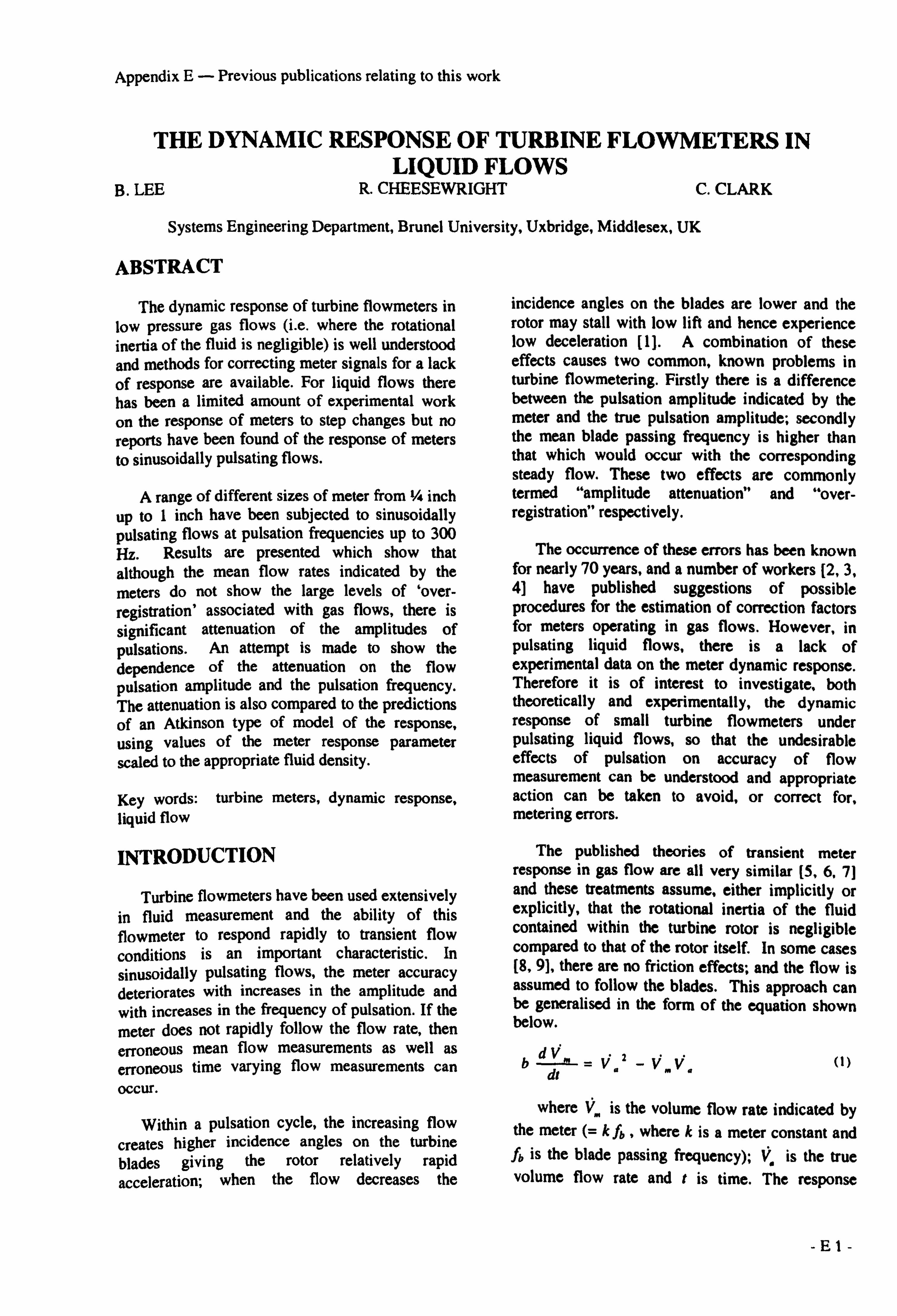
Appendix E- Previous publications relating to this work
THE DYNAMIC RESPONSE OF TURBINE FLOWMETERS IN
B. LEE LIQUID FLOWS
R. CHEESEWRIGHT C. CLARK
Systems Engineering Department, Brunel University, Uxbridge, Middlesex, UK
ABSTRACT
The dynamic response of turbine flowmeters in low pressure gas flows (i. e. where the rotational inertia of the fluid is negligible) is well understood and methods for correcting meter signals for a lack
of response are available. For liquid flows there has been a limited amount of experimental work on the response of meters to step changes but no reports have been found of the response of meters to sinusoidally pulsating flows.
A range of different sizes of meter from V inch
up to 1 inch have been subjected to sinusoidally pulsating flows at pulsation frequencies up to 300 Hz. Results are presented which show that although the mean flow rates indicated by the meters do not show the large levels of 'over-
registration' associated with gas flows, there is
significant attenuation of the amplitudes of pulsations. An attempt is made to show the dependence of the attenuation on the flow
pulsation amplitude and the pulsation frequency. The attenuation is also compared to the predictions of an Atkinson type of model of the response, using values of the meter response parameter scaled to the appropriate fluid density.
Key words: turbine meters, dynamic response, liquid flow
INTRODUCTION
Turbine flowmeters have been used extensively in fluid measurement and the ability of this flowmeter to respond rapidly to transient flow
conditions is an important characteristic. In
sinusoidally pulsating flows, the meter accuracy deteriorates with increases in the amplitude and with increases in the frequency of pulsation. If the
meter does not rapidly follow the flow rate, then
erroneous mean flow measurements as well as erroneous time varying flow measurements can occur.
Within a pulsation cycle, the increasing flow
creates higher incidence angles on the turbine blades giving the rotor relatively rapid acceleration; when the flow decreases the
incidence angles on the blades are lower and the rotor may stall with low lift and hence experience low deceleration [1]. A combination of these effects causes two common, known problems in turbine flowmetering. Firstly there is a difference between the pulsation amplitude indicated by the meter and the true pulsation amplitude; secondly the mean blade passing frequency is higher than that which would occur with the corresponding steady flow. These two effects are commonly termed "amplitude attenuation" and "over- registration" respectively.
The occurrence of these errors has been known for nearly 70 years, and a number of workers [2,3, 4] have published suggestions of possible procedures for the estimation of correction factors for meters operating in gas flows. However, in pulsating liquid flows, there is a lack of experimental data on the meter dynamic response. Therefore it is of interest to investigate, both theoretically and experimentally, the dynamic response of small turbine flowmeters under pulsating liquid flows, so that the undesirable effects of pulsation on accuracy of flow measurement can be understood and appropriate action can be taken to avoid, or correct for, metering errors.
The published theories of transient meter response in gas flow are all very similar [5,6.7] and these treatments assume, either implicitly or explicitly, that the rotational inertia of the fluid contained within the turbine rotor is negligible compared to that of the rotor itself. In some cases [8,9], there are no friction effects; and the flow is assumed to follow the blades. This approach can be generalised in the form of the equation shown below.
bdd _V 2_ý/�, i/a (1)
where V. is the volume flow rate indicated by the meter (= k fb , where k is a meter constant and fb is the blade passing frequency); V. is the true volume flow rate and t is time. The response
- EI -
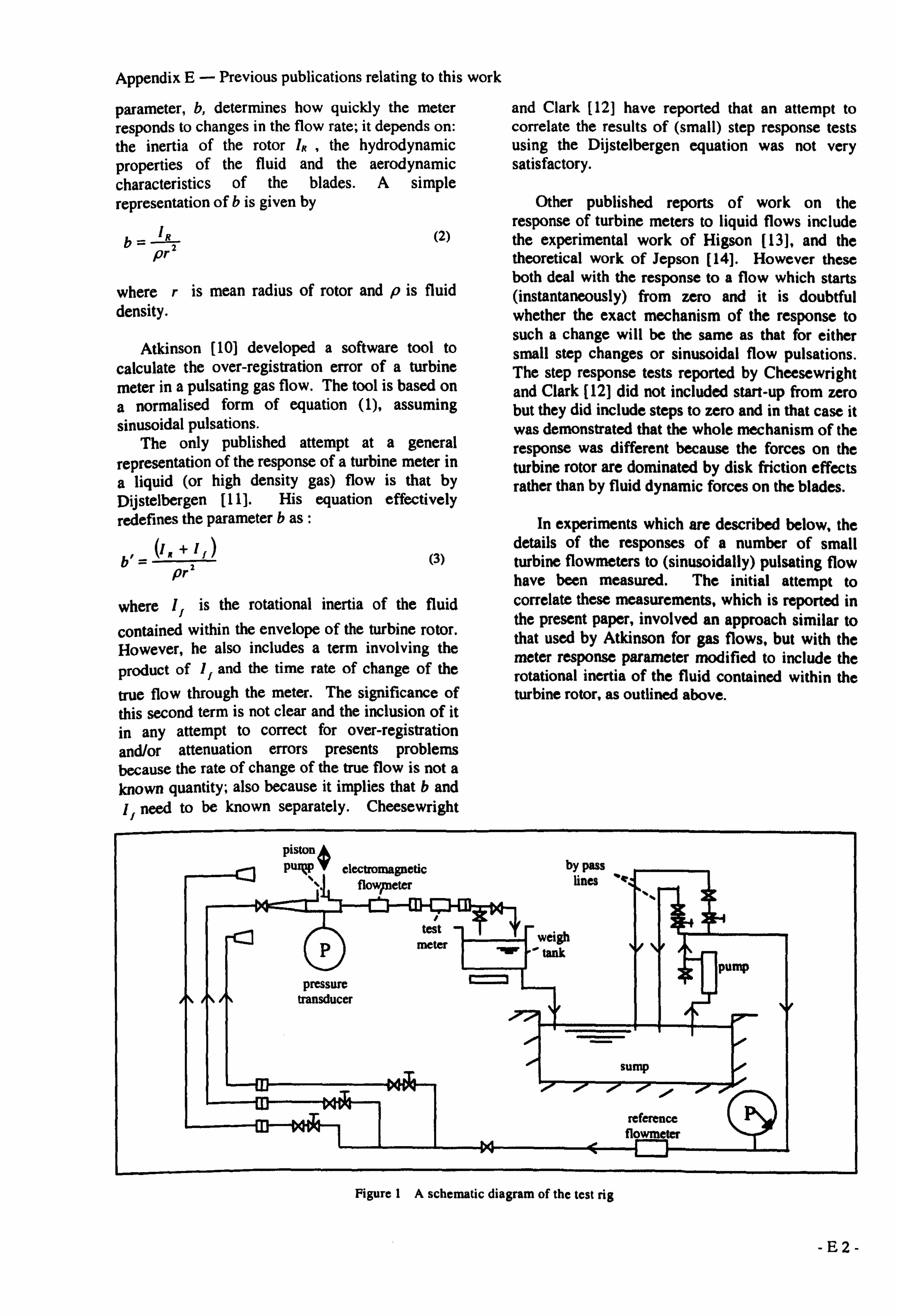
Appendix E- Previous publications relating to this work
parameter, b, determines how quickly the meter responds to changes in the flow rate; it depends on: the inertia of the rotor IR
, the hydrodynamic
properties of the fluid and the aerodynamic characteristics of the blades. A simple representation of b is given by
b=1- (2) pr
where r is mean radius of rotor and p is fluid density.
Atkinson [10] developed a software tool to calculate the over-registration error of a turbine meter in a pulsating gas flow. The tool is based on a normalised form of equation (1), assuming sinusoidal pulsations.
The only published attempt at a general representation of the response of a turbine meter in
a liquid (or high density gas) flow is that by Dijstelbergen [11]. His equation effectively redefines the parameter b as :
11. + b=Z (3)
pr
where If is the rotational inertia of the fluid
contained within the envelope of the turbine rotor. However, he also includes a term involving the
product of If and the time rate of change of the
true flow through the meter. The significance of this second term is not clear and the inclusion of it in any attempt to correct for over-registration and/or attenuation errors presents problems because the rate of change of the true flow is not a known quantity; also because it implies that b and 1j need to be known separately. Cheesewright
and Clark [12] have reported that an attempt to correlate the results of (small) step response tests using the Dijstelbergen equation was not very satisfactory.
Other published reports of work on the response of turbine meters to liquid flows include the experimental work of Higson [13], and the theoretical work of Jepson [14]. However these both deal with the response to a flow which starts (instantaneously) from zero and it is doubtful whether the exact mechanism of the response to such a change will be the same as that for either small step changes or sinusoidal flow pulsations. The step response tests reported by Cheesewright and Clark [12] did not included start-up from zero but they did include steps to zero and in that case it was demonstrated that the whole mechanism of the response was different because the forces on the turbine rotor are dominated by disk friction effects rather than by fluid dynamic forces on the blades.
In experiments which are described below, the details of the responses of a number of small turbine flowmeters to (sinusoidally) pulsating flow have been measured. The initial attempt to correlate these measurements, which is reported in the present paper, involved an approach similar to that used by Atkinson for gas flows, but with the meter response parameter modified to include the rotational inertia of the fluid contained within the turbine rotor, as outlined above.
piston A PWQP electromagnetic by pass
flowfneter lines
test P meter weigh
pump pressure
'9w -
transducer
-ol
sump
reference flowmeter
Figure 1A schematic diagram of the test rig
-E2-
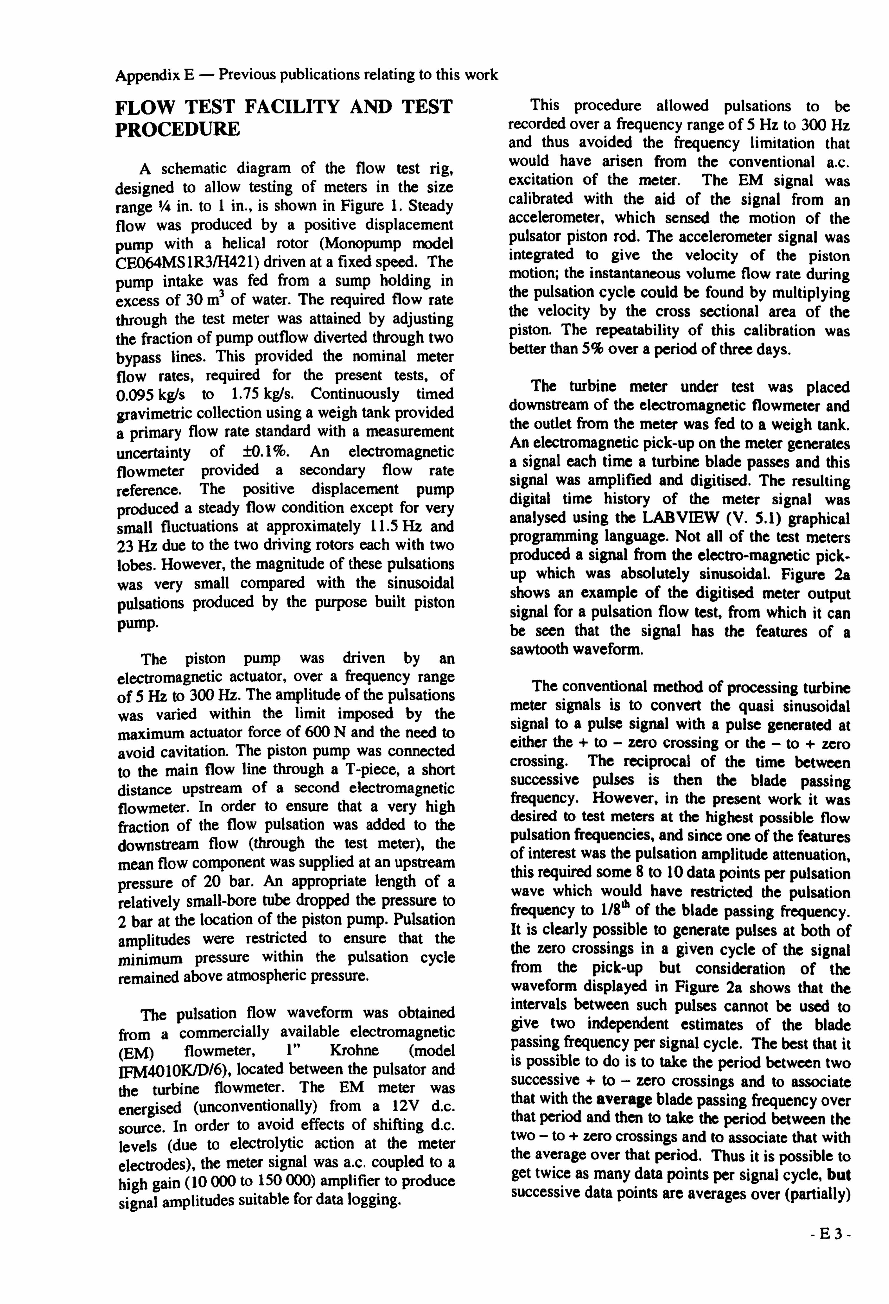
Appendix E- Previous publications relating to this work
FLOW TEST FACILITY AND TEST PROCEDURE
A schematic diagram of the flow test rig, designed to allow testing of meters in the size range 1/a in. to 1 in., is shown in Figure 1. Steady flow was produced by a positive displacement
pump with a helical rotor (Monopump model CE064MS1R3/H421) driven at a fixed speed. The
pump intake was fed from a sump holding in
excess of 30 m3 of water. The required flow rate through the test meter was attained by adjusting the fraction of pump outflow diverted through two bypass lines. This provided the nominal meter flow rates, required for the present tests, of 0.095 kg/s to 1.75 kg/s. Continuously timed gravimetric collection using a weigh tank provided a primary flow rate standard with a measurement uncertainty of ±0.1%. An electromagnetic flowmeter provided a secondary flow rate reference. The positive displacement pump produced a steady flow condition except for very small fluctuations at approximately 11.5 Hz and 23 Hz due to the two driving rotors each with two lobes. However, the magnitude of these pulsations was very small compared with the sinusoidal pulsations produced by the purpose built piston pump.
The piston pump was driven by an electromagnetic actuator, over a frequency range of 5 Hz to 300 Hz. The amplitude of the pulsations was varied within the limit imposed by the maximum actuator force of 600 N and the need to avoid cavitation. The piston pump was connected to the main flow line through a T-piece, a short distance upstream of a second electromagnetic flowmeter. In order to ensure that a very high fraction of the flow pulsation was added to the downstream flow (through the test meter), the mean flow component was supplied at an upstream pressure of 20 bar. An appropriate length of a relatively small-bore tube dropped the pressure to 2 bar at the location of the piston pump. Pulsation
amplitudes were restricted to ensure that the
minimum pressure within the pulsation cycle remained above atmospheric pressure.
The pulsation flow waveform was obtained from a commercially available electromagnetic (EM) flowmeter, 1" Krohne (model IFM401OK/D/6), located between the pulsator and the turbine flowmeter. The EM meter was energised (unconventionally) from a 12V d. c. source. In order to avoid effects of shifting d. c. levels (due to electrolytic action at the meter electrodes), the meter signal was a. c. coupled to a high gain (10 000 to 150 000) amplifier to produce signal amplitudes suitable for data logging.
This procedure allowed pulsations to be recorded over a frequency range of 5 Hz to 300 Hz and thus avoided the frequency limitation that would have arisen from the conventional a. c. excitation of the meter. The EM signal was calibrated with the aid of the signal from an accelerometer, which sensed the motion of the pulsator piston rod. The accelerometer signal was integrated to give the velocity of the piston motion; the instantaneous volume flow rate during the pulsation cycle could be found by multiplying the velocity by the cross sectional area of the piston. The repeatability of this calibration was better than 5% over a period of three days.
The turbine meter under test was placed downstream of the electromagnetic flowmeter and the outlet from the meter was fed to a weigh tank. An electromagnetic pick-up on the meter generates a signal each time a turbine blade passes and this signal was amplified and digitised. The resulting digital time history of the meter signal was analysed using the LABVIEW (V. 5.1) graphical programming language. Not all of the test meters produced a signal from the electro-magnetic pick- up which was absolutely sinusoidal. Figure 2a shows an example of the digitised meter output signal for a pulsation flow test, from which it can be seen that the signal has the features of a sawtooth waveform.
The conventional method of processing turbine meter signals is to convert the quasi sinusoidal signal to a pulse signal with a pulse generated at either the + to - zero crossing or the - to + zero crossing. The reciprocal of the time between successive pulses is then the blade passing frequency. However, in the present work it was desired to test meters at the highest possible flow pulsation frequencies, and since one of the features of interest was the pulsation amplitude attenuation, this required some 8 to 10 data points per pulsation wave which would have restricted the pulsation frequency to 1/8s' of the blade passing frequency. It is clearly possible to generate pulses at both of the zero crossings in a given cycle of the signal from the pick-up but consideration of the waveform displayed in Figure 2a shows that the intervals between such pulses cannot be used to give two independent estimates of the blade passing frequency per signal cycle. The best that it is possible to do is to take the period between two successive + to - zero crossings and to associate that with the average blade passing frequency over that period and then to take the period between the two - to + zero crossings and to associate that with the average over that period. Thus it is possible to get twice as many data points per signal cycle, but successive data points are averages over (partially)
-E3-
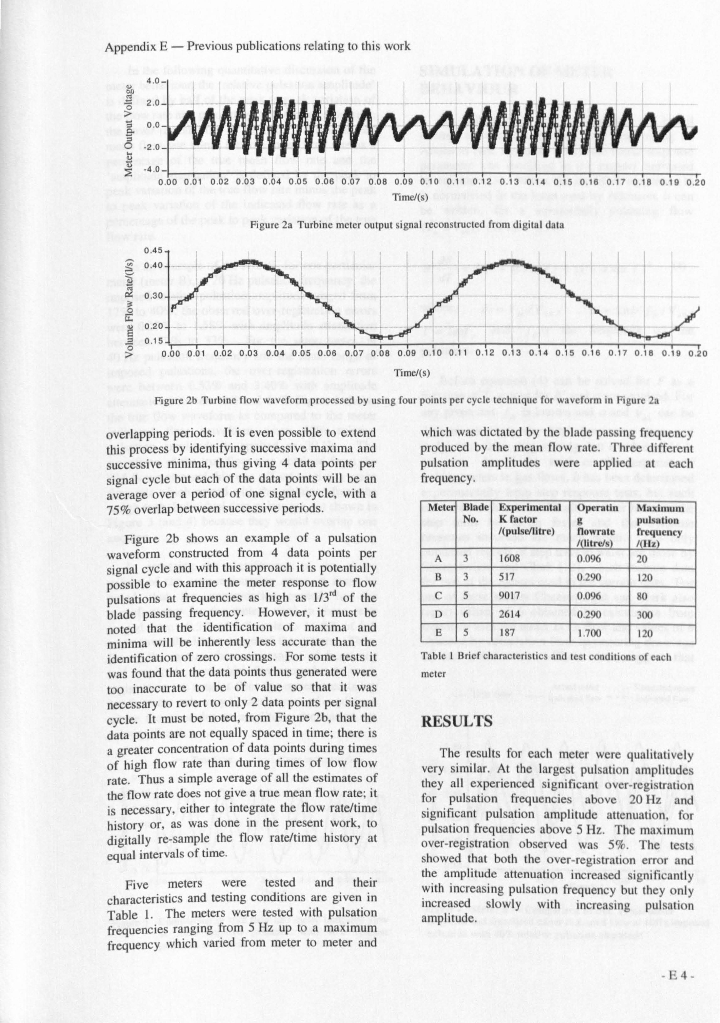
Appendix E- Previous publications relating to this work
4.0 00
= 2.0
0
0.0
-2.0 v
-4.0
Time/(s)
Figure 2a Turbine meter output signal reconstructed from digital data
0.45 0.40
0.30
0 0.20
0.15 Ö
Time/(s)
Figure 2b Turbine flow waveform processed by using four points per cycle technique for waveform in Figure 2a
overlapping periods. It is even possible to extend this process by identifying successive maxima and successive minima, thus giving 4 data points per signal cycle but each of the data points will be an average over a period of one signal cycle, with a 75% overlap between successive periods.
Figure 2b shows an example of a pulsation waveform constructed from 4 data points per signal cycle and with this approach it is potentially possible to examine the meter response to flow
pulsations at frequencies as high as 1/3rd of the blade passing frequency. However, it must be
noted that the identification of maxima and minima will be inherently less accurate than the identification of zero crossings. For some tests it
was found that the data points thus generated were too inaccurate to be of value so that it was necessary to revert to only 2 data points per signal cycle. It must be noted, from Figure 2b, that the data points are not equally spaced in time; there is
a greater concentration of data points during times
of high flow rate than during times of low flow
rate. Thus a simple average of all the estimates of the flow rate does not give a true mean flow rate; it is necessary, either to integrate the flow rate/time history or, as was done in the present work, to digitally re-sample the flow rate/time history at equal intervals of time.
Five meters were tested and their
characteristics and testing conditions are given in Table 1. The meters were tested with pulsation frequencies ranging from 5 Hz up to a maximum frequency which varied from meter to meter and
which was dictated by the blade passing frequency produced by the mean flow rate. Three different pulsation amplitudes were applied at each frequency.
Mete Blade No.
Experimental K factor /(pulsellitre)
Operatin g flowrate /(litres)
Maximum pulsation frequency / Ilz
A 3 1608 0.0% 20
B 3 517 0.290 120
C 5 9017 0.096 80
D 6 2614 0.290 300 E 5 187 1.700 120
Table I Brief characteristics and test conditions of each
meter
RESULTS
The results for each meter were qualitatively very similar. At the largest pulsation amplitudes they all experienced significant over-registration for pulsation frequencies above 20 Hz and significant pulsation amplitude attenuation, for pulsation frequencies above 5 Hz. The maximum over-registration observed was 5%. The tests showed that both the over-registration error and the amplitude attenuation increased significantly with increasing pulsation frequency but they only increased slowly with increasing pulsation amplitude.
-I 4-
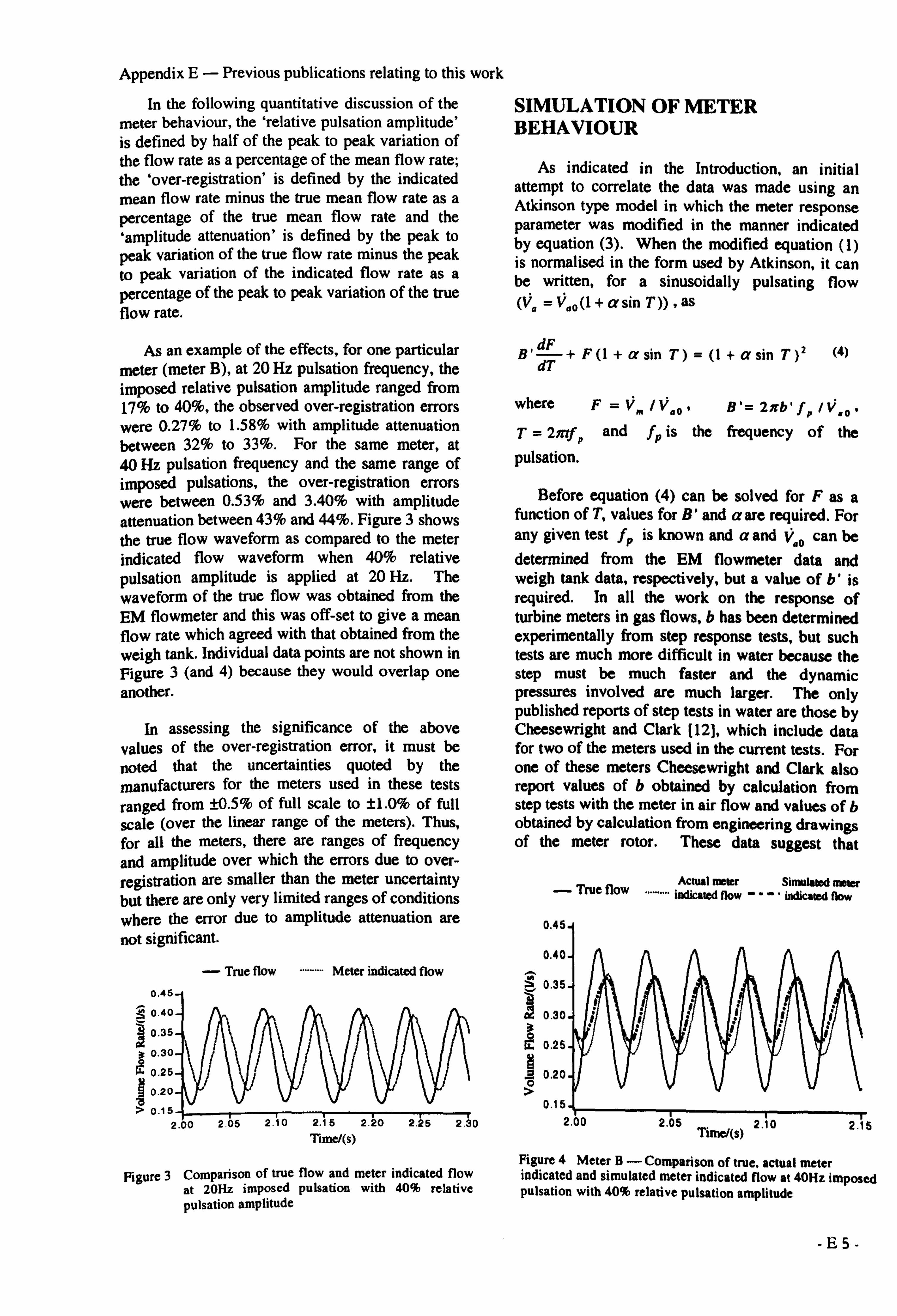
Appendix E- Previous publications relating to this work
In the following quantitative discussion of the meter behaviour, the `relative pulsation amplitude' is defined by half of the peak to peak variation of the flow rate as a percentage of the mean flow rate; the `over-registration' is defined by the indicated
mean flow rate minus the true mean flow rate as a percentage of the true mean flow rate and the `amplitude attenuation' is defined by the peak to peak variation of the true flow rate minus the peak to peak variation of the indicated flow rate as a percentage of the peak to peak variation of the true flow rate.
As an example of the effects, for one particular meter (meter B), at 20 Hz pulsation frequency, the imposed relative pulsation amplitude ranged from 17% to 40%, the observed over-registration errors were 0.27% to 1.58% with amplitude attenuation between 32% to 33%. For the same meter, at 40 Hz pulsation frequency and the same range of imposed pulsations, the over-registration errors were between 0.53% and 3.40% with amplitude attenuation between 43% and 44%. Figure 3 shows the true flow waveform as compared to the meter indicated flow waveform when 40% relative pulsation amplitude is applied at 20 Hz. The
waveform of the true flow was obtained from the EM flowmeter and this was off-set to give a mean flow rate which agreed with that obtained from the weigh tank. Individual data points are not shown in Figure 3 (and 4) because they would overlap one another.
In assessing the significance of the above values of the over-registration error, it must be
noted that the uncertainties quoted by the manufacturers for the meters used in these tests
ranged from ±0.5% of full scale to ±1.0% of full
scale (over the linear range of the meters). Thus, for all the meters, there are ranges of frequency
and amplitude over which the errors due to over- registration are smaller than the meter uncertainty but there are only very limited ranges of conditions where the error due to amplitude attenuation are not significant.
Timet(s)
Figure 3 Comparison of true flow and meter indicated flow at 20Hz imposed pulsation with 40% relative pulsation amplitude
SIMULATION OF METER BEHAVIOUR
As indicated in the Introduction, an initial attempt to correlate the data was made using an Atkinson type model in which the meter response parameter was modified in the manner indicated by equation (3). When the modified equation (1) is normalised in the form used by Atkinson, it can be written, for a sinusoidally pulsating flow (V, = V,
o (I +a sin T)) , as
B' +F(1+asin T)=(1+asin T)2 (4)
where F=V. /Vao, B'= 2irb' fo /V, 0. T= 2mf,, and fp is the frequency of the
pulsation.
Before equation (4) can be solved for F as a function of T, values for B' and a are required. For any given test fp is known and a and V.
0 can be determined from the EM flowmeter data and weigh tank data, respectively, but a value of b' is required. In all the work on the response of turbine meters in gas flows, b has been determined experimentally from step response tests, but such tests are much more difficult in water because the step must be much faster and the dynamic pressures involved are much larger. The only published reports of step tests in water are those by Cheesewright and Clark [12), which include data for two of the meters used in the current tests. For one of these meters Cheesewright and Clark also report values of b obtained by calculation from step tests with the meter in air flow and values of b obtained by calculation from engineering drawings of the meter rotor. These data suggest that
- True flow Actual meter Simulaled meter
indicated flow ---" indicated flow
a_
3
I
0
0.45
0.40
0.35
0.30
0.25
0.20
0.15
'lime/(S) Figure 4 Meter B- Comparison of true, actual meter indicated and simulated meter indicated flow at 40Hz imposed pulsation with 40% relative pulsation amplitude
-E5-
- True flow "°°°°" Meter indicated flow
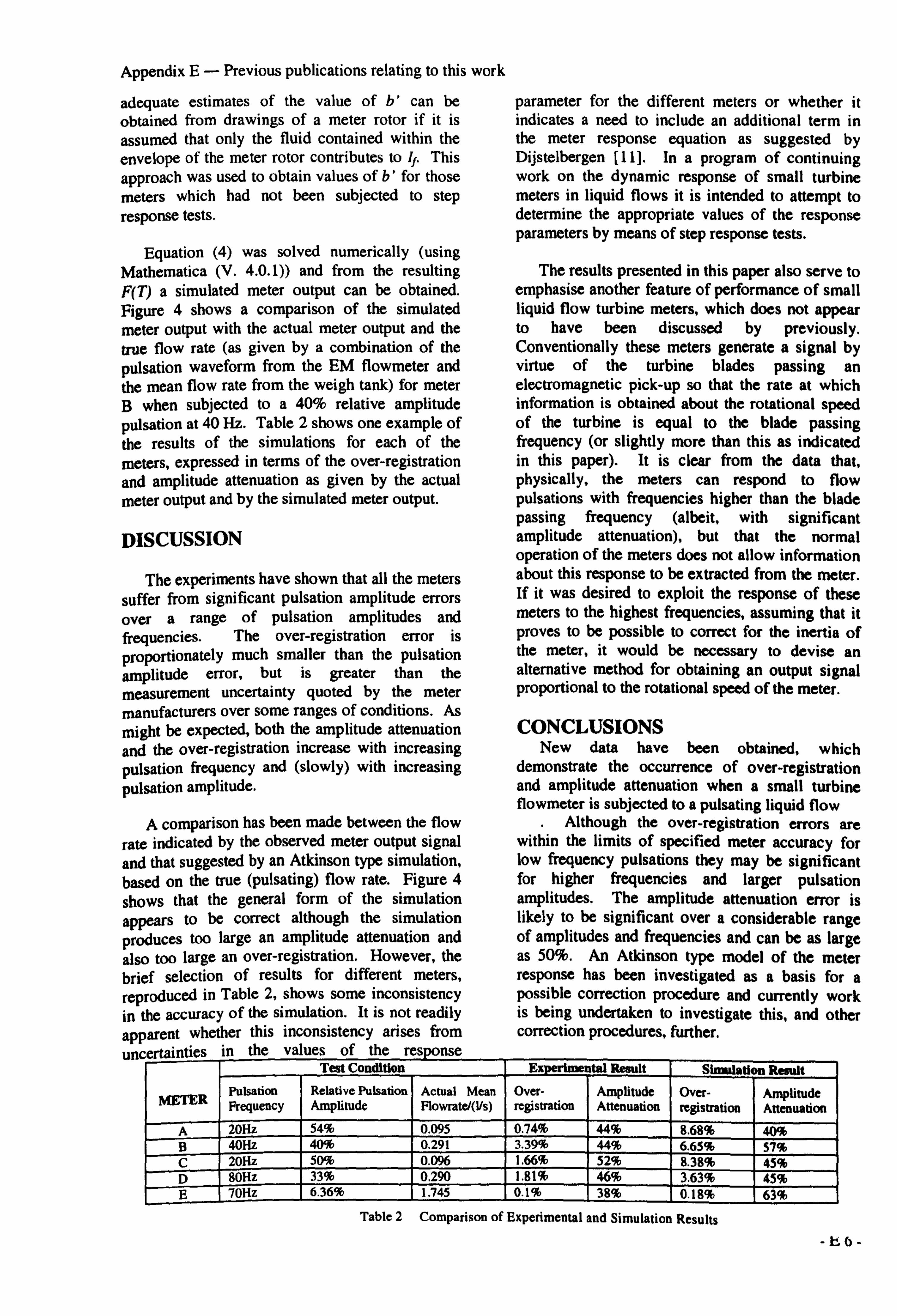
Appendix E- Previous publications relating to this work
adequate estimates of the value of b' can be
obtained from drawings of a meter rotor if it is
assumed that only the fluid contained within the envelope of the meter rotor contributes to If. This
approach was used to obtain values of b' for those meters which had not been subjected to step response tests.
Equation (4) was solved numerically (using Mathematica (V. 4.0.1)) and from the resulting F(T) a simulated meter output can be obtained. Figure 4 shows a comparison of the simulated meter output with the actual meter output and the true flow rate (as given by a combination of the pulsation waveform from the EM flowmeter and the mean flow rate from the weigh tank) for meter B when subjected to a 40% relative amplitude pulsation at 40 Hz. Table 2 shows one example of the results of the simulations for each of the meters, expressed in terms of the over-registration and amplitude attenuation as given by the actual meter output and by the simulated meter output.
DISCUSSION
The experiments have shown that all the meters suffer from significant pulsation amplitude errors over a range of pulsation amplitudes and frequencies. The over-registration error is
proportionately much smaller than the pulsation amplitude error, but is greater than the measurement uncertainty quoted by the meter manufacturers over some ranges of conditions. As
might be expected, both the amplitude attenuation and the over-registration increase with increasing
pulsation frequency and (slowly) with increasing
pulsation amplitude.
A comparison has been made between the flow
rate indicated by the observed meter output signal and that suggested by an Atkinson type simulation, based on the true (pulsating) flow rate. Figure 4
shows that the general form of the simulation appears to be correct although the simulation produces too large an amplitude attenuation and also too large an over-registration. However, the brief selection of results for different meters, reproduced in Table 2, shows some inconsistency in the accuracy of the simulation. It is not readily apparent whether this inconsistency arises from
uncertainties in the values of the response
parameter for the different meters or whether it indicates a need to include an additional term in the meter response equation as suggested by Dijstelbergen [11]. In a program of continuing work on the dynamic response of small turbine meters in liquid flows it is intended to attempt to determine the appropriate values of the response parameters by means of step response tests.
The results presented in this paper also serve to emphasise another feature of performance of small liquid flow turbine meters, which does not appear to have been discussed by previously. Conventionally these meters generate a signal by virtue of the turbine blades passing an electromagnetic pick-up so that the rate at which information is obtained about the rotational speed of the turbine is equal to the blade passing frequency (or slightly more than this as indicated in this paper). It is clear from the data that, physically, the meters can respond to flow pulsations with frequencies higher than the blade passing frequency (albeit, with significant amplitude attenuation), but that the normal operation of the meters does not allow information about this response to be extracted from the meter. If it was desired to exploit the response of these meters to the highest frequencies, assuming that it proves to be possible to correct for the inertia of the meter, it would be necessary to devise an alternative method for obtaining an output signal proportional to the rotational speed of the meter.
CONCLUSIONS New data have been obtained, which
demonstrate the occurrence of over-registration and amplitude attenuation when a small turbine flowmeter is subjected to a pulsating liquid flow
. Although the over-registration errors are within the limits of specified meter accuracy for low frequency pulsations they may be significant for higher frequencies and larger pulsation amplitudes. The amplitude attenuation error is likely to be significant over a considerable range of amplitudes and frequencies and can be as large as 50%. An Atkinson type model of the meter response has been investigated as a basis for a possible correction procedure and currently work is being undertaken to investigate this, and other correction procedures, further.
Test Condition Ex tsl Result Simulation Result
NEMR Pulsation Frequency
Relative Pulsation Amplitude
Actual Mean Flowrate/(Vs)
Over- registration
Amplitude Attenuation
Over- registration
Amplitude Attenuation
A 20Hz 54% 0.095 0.74% 44% 8.68% 40% B 40Hz 40% 0.291 3.39% 44% 6.65% 57% C 20Hz 50% 0.096 1.66% 52% 8.38% 45% D 80Hz 33% 0.290 1.81% 46% 3.63% 45% E 70Hz 6.36% 1.745 0.1% 38% 0.18% 63%
Table 2 Comparison of Experimental and Simulation Results
-h6-
Appendix E- Previous publications relating to this work
ACKNOWLEGEMENT
The experimental work and part of the input from the second author were supported by a grant from the UK Engineering and Physical Sciences Research Council.
REFERENCES
[1] R. C. Baker, Turbine flowmeters: II. Theoretical and experimental published information, Flow Meas. Instrum., 4(3), 1993, 123-144. [2] E. Ower, On the response of a vane anemometer to an air-stream of pulsating speed, Phil. Mag., 7(23), 1937,992-1004.
[31 W. F. Z. Lee, M. J. Kirik, J. A. Bonner, Gas turbine flowmeter measurement of pulsating flow, J. Engineering for Power, Trans. ASME, October, 1975,531-539.
[4] J. W. Bronner and R. J. McKee, Cogen
pulsation effects on turbine metering, American Gas Association, Operating Section, Proceedings, 1991,625-638.
[51 J. Grey, Transient response of the turbine flowmeter, Jet Propulsion, February, 1956,98- 100.
[6] W. F. Z. Lee and H. J. Evans, A field method of determining gas turbine meter performance, J. Basic Eng. Trans. ASME, December, 1970,717- 728.
[7] R. Cheesewright, D. Edwards and C. Clark, Measurements with a turbine flow meter in the presence of large, non-sinusoidal pulsations, Proc. FLUCOME '94, Toulouse, France, August, 1994.
[81 R. J. McKee, Pulsation effects on single- and two-rotor turbine meters, Flow Meas. Instrum., 3(3), 1992,151-166.
[9] R. Cheesewright et al, Field tests of correction procedures for turbine flowmeters in pulsatile flows, Flow Meas. Instrum., 7(1), 1996,7-17.
[10] K. N. Atkinson, A software tool to calculate the over-registration error of a turbine meter in pulsating flow, Flow Meas. Instrum., 3(3), 1992, 167-172.
[11] H. H. Dijstelbergen, Rotameters and turbine flowmeters in pulsation flow measurement, Measurement and Control, 3, December, 1970,
197-204.
[12] R. Cheesewright and C. Clark, Step response tests on turbine flowmeters in liquid flows, Proc. Instn. Mech. Engrs., 211(A), 1997,321-330.
[13) D. J. Higson, The transient performance of turbine flowmeters in water, J. Sci Instrum., 42(5), 1964,337-342.
[14] P. Jepson, Transient response of a helical flowmeter, J. Mech. Eng. Sci., 6(4), 1964,337- 342.
-E7-