Embed Size (px)
Citation preview

Demography, Volume 46-Number 3, August 2009: 589–603 589
D
DRAWING STATISTICAL INFERENCES FROM HISTORICAL CENSUS DATA, 1850–1950*
MICHAEL DAVERN, STEVEN RUGGLES, TAMI SWENSON, J. TRENT ALEXANDER, AND J. MICHAEL OAKES
Virtually all quantitative microdata used by social scientists derive from samples that incorporate clustering, stratifi cation, and weighting adjustments (Kish 1965, 1992). Such data can yield standard error estimates that differ dramatically from those derived from a simple random sample of the same size. Researchers using historical U.S. census microdata, however, usually apply methods designed for simple random samples. The resulting p values and confi dence intervals could be inaccurate and could lead to erroneous research conclusions. Because U.S. census microdata samples are among the most widely used sources for social science and policy research, the need for reliable standard error estimation is critical. We evaluate the historical microdata samples of the Integrated Public Use Microdata Series (IPUMS) project from 1850 to 1950 in order to determine (1) the impact of sample design on standard error estimates, and (2) how to apply modern standard error estimation software to historical census samples. We exploit a unique new data source from the 1880 census to validate our methods for standard error estimation, and then we apply this approach to the 1850–1870 and 1900–1950 decennial censuses. We conclude that Taylor series estimation can be used effectively with the historical decennial census microdata samples and should be applied in research analyses that have the potential for substantial clustering effects.
ecennial census microdata are a key component of social science infrastructure. Census microdata are among the most frequently used data sources in the leading journals of popu-lation, economics, and sociology; indeed, during the past decade, census microdata have been used more frequently in the pages of Demography than any other data source.1 Most of these publications have used the Integrated Public Use Microdata Series (IPUMS), which makes freely available to scholars large, nationally representative samples of every surviv-ing census from 1850 though 2000; these data are in harmonized format and are available through a user-friendly data access system with comprehensive documentation (Ruggles et al. 2004). Since 1995, more than 25,000 researchers have registered to use the IPUMS data extraction system, and they have produced 2,000 publications and working papers.
Census microdata samples are individual-level data clustered by household, often incorporate stratifi cation, and sometimes use differential probabilities of selection (in addition to differential nonresponse), resulting in heterogeneity in sample weights. The clustering of individuals within households can signifi cantly increase standard errors of estimates because the number of independent observations is less than the number of actual observations in each census fi le. Standard errors in cluster samples depend on both the size of the sampled clusters and the homogeneity of variables within clusters, measured by an intraclass correlation coeffi cient (Graubard and Korn 1996; Hansen, Hurwitz, and Madow 1953; Kish 1992; Korn and Graubard 1995, 1999). In the worst case, with perfect homo-geneity within clusters, the standard errors for variables would be inversely proportional to the square root of the number of clusters rather than the number of people. Thus, variables
*Michael Davern, Steven Ruggles, Tami Swenson, J. Trent Alexander, and J. Michael Oakes, Minnesota Population Center, University of Minnesota. Address correspondence to Michael Davern, SHADAC, University of Minnesota, 2221 University Avenue SE, Suite 345, Minneapolis, MN 55414; e-mail: [email protected]. This research was supported by Grant Number R01 HD043392-03S1 from the National Institute of Child Health and Development of the National Institutes of Health.
1. In the decade from 1997 through 2006, U.S. census microdata were used in 54 Demography articles, substantially more than any other data source.

590 Demography, Volume 46-Number 3, August 2009
such as race and poverty status, which tend to be comparatively homogeneous within households, have underestimated standard errors if clustering was ignored. Conversely, for variables that are heterogeneous within clusters, such as age and sex, clustering may have little effect on sample precision.
The loss of effi ciency resulting from clustered design is partially counterbalanced by stratifi cation (Kish 1992). The IPUMS samples for the years prior to 1960 were designed to capitalize on geographically sorted source materials, which enhance precision through implicit geographic stratifi cation. Such procedures can lower standard errors, especially for variables that are highly correlated with geography
In this article, we examine the impact of complex sample designs on standard error estimates using IPUMS historical U.S. census microdata samples for 1850 through 1950. We compare standard errors computed using a simple random sampling assumption––the usual way of computing standard errors using the historical U.S. census data––with esti-mates that take the complex sample design into account. We develop and test a new variable that allows us to apply modern standard error estimation software to IPUMS census micro-data. Based on the results of this evaluation, we develop recommendations for standard error estimation when using the IPUMS samples from 1850 through 1950.2
METHODSSophisticated methods for standard error estimation are now available in easy-to-use procedures in statistical packages. In particular, Taylor series estimation procedures are now incorporated into most statistical analysis packages (SAS 1999; Stata 2001; SPSS 2003), and these procedures yield reliable estimates (Dippo and Wolter 1984; Hammer, Shin, and Porcellini 2003; Kish and Frankel 1974; Krewski and Rao 1981; Weng, Zhang, and Cohen 1995). Researchers frequently use these products for analysis of survey data, but they are seldom applied to decennial census microdata. In part, this is because the census microdata samples do not include all the variables required to take advantage of the new software algorithms.
Implicit Geographic Stratifi cationThe source materials for the IPUMS samples of the pre-1960 censuses are the census enu-merators’ manuscripts, which had a similar format from 1850 though 1950. A sample page from the census of 1930 appears in Figure 1. Each line represents one individual, and for most census years, there are 50 lines on each page. Enumerators identifi ed the divisions between one dwelling or household and the next by numbering each unit and identifying the head of each household in the family relationship fi eld. The criteria used to distinguish between households were closely comparable across the entire period from 1850 to 2000 (Ruggles and Brower 2003).
The enumerators collected census information by going from house to house. Each enumerator was responsible for one enumeration district. In most census years, the aver-age district included between 1,000 and 1,500 persons (Magnuson 1995; Magnuson and King 1995). Urban districts tended to be compact, but rural ones could be geographically extensive, especially in sparsely settled places.
The publicly available IPUMS samples created at the University of Minnesota for the censuses of 1850 through 1930 all employ the same basic design, with minor variations to accommodate differences in source materials and innovations in data-entry technology.
2. We reviewed 20 recent articles in Demography that used the 1850–1950 microdata for original analysis (the full set of references is in the appendix), and none of them mention having adjusted standard errors for household clustering and stratifi cation even though this functionality is available in most modern statistical packages (e.g., SPSS, SAS, and Stata). This does not mean these articles made invalid inferences; as discussed later, for many analyses, ignoring the effects of clustering and stratifi cation can yield conservative variance estimates.

Drawing Statistical Inferences From Historical Census Data 591
Figu
re 1
. 19
30 C
ensu
s Enu
mer
atio
n Fo
rm

592 Demography, Volume 46-Number 3, August 2009
The sampling strategy is based on the census page. We generate a random starting point for each microfi lm reel between 1 and 5, and then designate every 10th page thereafter as a sample page. Thus, for example, if the starting point is 3, we designate the 3rd, 13th, and 23rd pages, continuing in that fashion until the end of the reel. On each sample page, we randomly select a set of sample points. The number of designated sample points de-pends on the desired sample density. For example, if the census page has 50 lines and a group of 10 pages therefore has 500 lines, we need to designate fi ve sample points on each sample page to obtain a 1% sample. To ensure that dwellings have an equal prob-ability of being included in the sample regardless of their size, they are entered only if a sample point falls on the line containing the fi rst person in the dwelling. When a sample point falls on any other dwelling member, the dwelling is skipped. For example, if the sample point falls within a dwelling of fi ve members, the dwelling will have only a one in fi ve chance of being included in the sample; if it is included, all fi ve members will be entered. Under this procedure, each dwelling, household, and individual in the population has exactly a 1-in-100 probability of inclusion.
We modify these procedures for persons residing in group quarters. We sample mem-bers of large units on an individual basis simply by treating each member as if he or she lived in his or her own one-person household. This procedure increases the effi ciency of the sample by raising the number of independent observations while maintaining rep-resentativeness. Without individual-level sampling of residents in group quarters, the precision of estimates for this population would be very low. In all the IPUMS samples between 1850 and 1930, large units are defi ned as households with more than 30 mem-bers. We sample within such households simply by accepting all individuals who fall on a sample point.
In 1940 and 1950, the sampling procedures were somewhat different, but the result was very similar. In 1940, the Census Bureau introduced the practice of asking extra questions of a sample of the population. Instead of asking the supplemental questions of an entire household, as was done for the censuses of 1960 through 2000, in 1940 and 1950, enumerators asked the questions of a systematic sample of individuals. The IPUMS samples were designed to ensure that every sampled household included a person who was asked the supplemental questions. Because larger households had a higher prob-ability of containing such a person, households were selected into the sample in inverse proportion to their size. Thus, all one-person households were included if the respondent was asked the extra questions, half the two-person households were included if either respondent had answered the questions, and so on. Data-entry staff consulted a random number table to determine if a household of a given size should be included. The effect of this procedure is very similar to taking households only if the sample point falls on the fi rst individual in the household. For 1950, the procedure was the same as for 1940, but without the control for household size: it is a fl at sample of all households containing an individual with extra questions. As a result, the 1950 sample overrepresents large house-holds and must be weighted to compensate.3
The sample designs for these early censuses differ fundamentally from those of the censuses of 1960 through 2000 because they were drawn from microfi lm images of the
3. There are several other differences between the 1850–1930 and the 1940–1950 designs. First, for 1940 and 1950, the basic sampling unit was the household. Before 1940, the basic sample unit was the dwelling, and because there were multiple sample points for each sampled page, occasionally more than one unit was sampled from the same enumeration page. Before 1940, group quarters units were defi ned as units with more than 30 members, and in 1940 and 1950 they were units with more than fi ve persons who were unrelated to the head of the household. Moreover, in the pre-1940 period, group quarters units were sampled in clusters of fi ve contigu-ous individuals; in 1940–1950, they were sampled as isolated individuals, eliminating clustering effects for residents in group quarters. See Ruggles et al. (2004) and Ruggles and Brower (2003) for a full description of differences between sample designs.

Drawing Statistical Inferences From Historical Census Data 593
original census enumerator manuscripts instead of from machine-readable fi les. Explicit stratifi cation was not feasible, but the organization of historical census enumeration forms incorporated implicit geographic stratifi cation. Unlike recent mail-in U.S. censuses, the pre-1960 censuses were created through direct enumeration: an enumerator went from house to house to interview residents in person. A byproduct of this enumeration method is that the census forms are sorted according to the sequence of enumeration within each enumeration district. In practice, this means that the enumeration manuscripts are geographically organized within districts.
The systematic samples of the historical censuses capitalize on this low-level geo-graphic sorting. By ensuring a representative geographic distribution of sampled cases, they are equivalent to extremely fi ne geographic stratifi cation with proportional weighting. Since many economic and demographic characteristics are highly correlated with geographic location, this implicit stratifi cation can yield substantially greater precision than a simple random sample of households. By capitalizing on implicit stratifi cation of the pages, this design yields higher precision for many estimates.
Pseudo-Strata and Taylor Series LinearizationTaylor series linearization is the easiest and most widely used method for estimating vari-ance with complex sample designs, but it is not designed for samples with implicit stratifi -cation. Because the stratifi cation in census records is implicit, there is no geographic unit in the data that corresponds precisely to the geographic stratifi cation embedded in the page ordering of the manuscripts. This poses a major problem for Taylor series linearization, since the method requires explicit information about strata.
To create a proxy for the implicit geographic stratifi cation of the historical IPUMS samples, we used the Census Bureau’s page numbering scheme in combination with explicit geographic information written on the census page. The manuscripts from each census are stored on several thousand microfi lm reels. Most reels contain several hundred pages. Each of these pages contains between 40 and 50 lines, with each line containing information on one person. For the samples from 1850–1930, we created pseudo-strata of approximately 10,000 lines. These pseudo-strata, on average, record information for about 2,000 households. We ensured that each stratum included cases from a single county; at each break between counties, we started a new stratum.4 For the 1940–1950 samples, we adopted a slightly different strategy, since we lack information on reel, page number, and most counties. We therefore defi ned strata as enumeration districts during these years. Enumeration districts consist of contiguous groups of neighborhoods or minor civil divi-sions. The specifi c boundaries of enumeration districts were defi ned as the area that a door-to-door enumerator could be expected to cover in a two-week period. Enumeration districts are consistently identifi ed in these samples.5
4. For this reason, some strata cover fewer than 10,000 lines. Strata that initially contained only a single sample household were allocated to other strata via a multistage procedure that takes advantage of geographic information we have about the household. Of the 2.5 million households in all of the 1850–1930 samples combined, only 4,200 were in one-household strata. If the household was in the same county as the previous or following stratum, we placed the household in that stratum. Almost 90% of these households were placed in this way. Oth-erwise, single-household strata were grouped with other single-household strata in the same State Economic Area (SEA); state; or, in a few cases, the entire country.
5. When enumeration districts had only one household in the sample, we created a merged stratum by combin-ing all single-household strata in the same SEA. The 1940 and 1950 data sets together had 852,164 households. Of those, 84,487 were the sole sampled household within their stratum. All of these cases were placed in SEA-level strata with others of their kind.

594 Demography, Volume 46-Number 3, August 2009
Subsample-Replicate Approach
An alternative to Taylor series variance estimation is the subsample-replicate approach (Rust 1985; Verma 1993; Wolter 1985).6 The replicate approach divides a sample into subsamples (or replicates) that refl ect the complex design of the entire sample. Each sub-sample incorporates the same stratifi cation and clustering used to select the sample as a whole.7 Iterative computer procedures are then used to estimate standard errors. It has not been established, however, whether the subsample replicate method is reliable for samples that incorporate implicit geographic stratifi cation. Subsample replicate estimates could be biased if the degree of geographic homogeneity varies greatly with geographic scale. For example, a typical 1-in-100 sample includes one household approximately every fi fth manuscript census page; if we divide that sample into 100 subsample replicates, however, cases occur only once every 500 pages and thus have high heterogeneity. This difference in geographic scale could have signifi cant implications for variance.
ValidationTo validate both the Taylor series linearization with pseudo-strata and the subsample-replicate approach, we needed a “true” estimate of variance in the census samples. Fortunately, a new source can provide near-perfect estimates for the 1880 census. The 1880 population database provides individual-level data on the entire population of 50 million Americans, assembled with the help of 11 million hours of volunteer effort by members of the Church of Jesus Christ of Latter-Day Saints (Goeken et al. 2003). This remarkable database provides an ideal laboratory for the evaluation of sample designs. The database allows us to simulate any sample design precisely, and by repeatedly draw-ing samples from the full 1880 census, we can develop highly accurate variance estimates for the IPUMS sample design.8 We can then compare these estimates with results based on both the IPUMS subsample replicates and Taylor series linearization to assess the reliability of both methods.
6. Statisticians are currently developing model-based variance estimates (e.g., Little 2003) to improve on the design-based variance estimates we examine, but there is not a specifi c algorithm available in statistical packages to implement them. The model-based variance estimates are beyond our current scope of work for two reasons: (1) the standards for implementing model-based variance estimates are not set for routine statistical analysis, and (2) it is still not clear how model-based variance estimates will be used for complex sample designs like the census (Kalton 2002).
7. The IPUMS subsample standard error estimates were calculated using the subsample variable on the 1850–1950 IPUMS 1% samples, which systematically divides the IPUMS sample into 100 replicate subsamples. For the historical IPUMS samples, the values are assigned sequentially from 0 to 99 for each dwelling or group quarters member. The IPUMS replicate standard errors are constructed by calculating the mean for each subsample separately and then averaging the 100 subsample means. The standard deviation of these 100 replicates is the IPUMS subsample-replicate standard error estimate.
8. The 1880 replicate reconstruction from the full 1880 census universe was completed using the household selection rules for the IPUMS 1880 1% sample (Ruggles and Menard 1995). In order to replicate the IPUMS sample design, we used the SAS procedure PROC SURVEYSELECT to randomly select one person per microfi lm page. This process was carried out for 100 replicate 1% samples, and the sampling rules determined the eligibility of the household or individual for inclusion in the fi nal sample. The sampling rules selected households or families if the randomly selected sample line was the household or family head and selected individuals for group quarters larger than 31 persons. If the randomly selected sample line did not meet the sampling rule criteria, the sample line was disregarded. We used PROC SURVEYSELECT to select 100 1% samples, following the IPUMS sampling rules from the full 1880 microdata census fi le (Ruggles and Menard 1995). The full 1880 census 1% sample replication has variance estimates that are on a different scale than the replications of the 1% IPUMS fi le, which are based on a sample of only 0.1% of the records. As a result, the full 1880 census 1% replication results are divided by the square root of 100 (i.e., 10) because the standard errors from the full 1880 census replication are based on samples that are 100 times larger than those based on the 1% IPUMS.

Drawing Statistical Inferences From Historical Census Data 595
RESULTS
Table 1 compares alternate methods for estimating standard errors of selected variables in the 1880 census. The fi rst two columns are based on sample replication of the entire 1880 population. We drew 100 independent 1% samples from the complete-count database, mim-icking the sample design used to create the historical samples. The standard errors derived from these replicates are unbiased estimates of the standard error that would be expected in a 1% sample.
The last three columns present the ratio of the standard error calculated from the 1% IPUMS sample for 1880 using three methods: subsample replicate, Taylor series linearization with pseudo-strata, and simple random sample assumptions to the standard error using the full 1880 census subsample replication. We regard the full 1880 census subsample replicates as a gold standard, so the ideal ratio would be 1.0. Ratios under 1.0 represent underestimated standard errors, and ratios over 1.0 represent overestimated standard errors.
The top row of Table 1 shows that in 1880, the average age was estimated to be 24.2 years, with a full census replication standard error estimate of 0.03. The ratio of the 1% IPUMS sample replicate to the full census replication was 1.1. The ratio for the Taylor series was 1.1, and the simple random sample was 0.9. These estimates are all quite close to one another, suggesting that for this variable, the particular method of standard error estimation does not matter much. This is not surprising, since age is not highly correlated within clusters (i.e., households) or by strata (i.e., geographic strata).
The poorest performing estimates in Table 1 were for the nonwhite and nonrelative simple random sample estimates, with a ratio of 0.5. When using statistics that assume a simple random sample, which is the default in most statistical packages, the standard error estimates would be about half as large as the standard errors that take the sample design into account. This is the result of household clustering; these characteristics were both highly correlated within households.
Table 1. Standard Error Computations Comparing Replicate Estimates From the Complete 1880 Census With Estimates Derived From Sample Data Using Alternative Methods
Ratio of Estimates Using the IPUMS 1880 1% Sample to Replicate Estimates Replicate From the Entire 1880 Census __________________________________________ Parameter Variance Estimates Taylor Series Estimate From Drawn From Subsample- Linearization SimpleSelected Person the Entire the Entire Replicate With RandomCharacteristics 1880 Census 1880 Census Method Psuedo-Strata Sample
Age (mean) 24.2 0.03 1.1 1.1 0.9 Male (%) 50.9 0.05 1.1 1.1 1.3 Married (%) 34.9 0.06 0.9 1.0 1.1 Nonwhite (%) 13.4 0.10 0.9 0.9 0.5 Foreign-born (%) 13.6 0.07 1.1 0.9 0.7 Socioeconomic Index (mean) 6.8 0.02 1.3 1.2 1.1 Other Relative (%) 5.3 0.04 1.1 1.2 0.8 Nonrelative (%) 9.7 0.08 0.9 0.9 0.5
Average 1.1 1.0 0.9
Source: 1880 full census and the 1880 IPUMS 1% sample.

596 Demography, Volume 46-Number 3, August 2009
For a few characteristics, the estimation methods overstate true standard error. This is most noticeable for the characteristic male. This variable varied greatly across geographic areas in 1880, so the implicit stratifi cation signifi cantly reduces standard errors. The other variance estimation methods pick this up, and the ratios reported in Table 1 are much closer to 1.
On the whole, however, the Taylor series and IPUMS 1% subsample-replicate estimates both performed well; the overall average ratios were 1.1 for the IPUMS 1% subsample-replicate estimates and 1.0 for the Taylor series estimates. By contrast, assuming a simple random sample leads to substantial underestimates of standard errors for several characteristics that are highly correlated within households.
When we turn to other historical samples from the IPUMS—1850, 1860, 1870, 1900, 1910, 1920, 1930, 1940, and 1950—we no longer have the gold standard of the full census replication because only the IPUMS sample data exist for those years. Table 2 therefore varies in structure from Table 1. The fi rst column contains the population parameter estimate from the IPUMS sample, and the second column contains the standard error estimates based on the assumption that the data were collected as a simple random sample. The remaining two columns present the Taylor series and subsample-replicate estimates as ratios to simple random sample estimates. A high ratio indicates that the standard error estimation method yields larger standard errors than would be obtained from a simple ran-dom sample of the same size.
The key fi nding is that the Taylor series estimates using the dwelling unit/household as the clustering variable and the stratifi cation variable we created based on sample pages (which allows us to recognize the implicit stratifi cation in the sample) yielded results for most of the domains examined in Table 2 that are very similar to those of the replicate estimates from the IPUMS samples. On average, the Taylor series and replicated estimates led to standard errors that were 1.4 times larger than the simple random sample estimates. When the ratio of the Taylor series estimates to the simple random sample estimates was below 1, the replicate estimates ratio also tended to be below 1 (and vice versa). The two approaches to estimating the standard errors yielded very similar results. The one exception is with the estimate of urban residence, in which the replicate estimates were consistently larger than the Taylor series across census years.
Several characteristics had consistently high ratios across all census years. In addition to nonwhite and nonrelative mentioned in the discussion of 1880, we examined two vari-ables with extremely high ratios: urban residence and farm residence. These are, in fact, household-level variables, not person-level variables, but we rectangularized the fi le and added the household-level characteristics to each person record to demonstrate the effects of clustering. Therefore, these two characteristics are identical for every individual in the household. With this perfect correlation, standard errors based on a simple random sample assumption are severely underestimated.
DISCUSSIONOur validation analysis using the 1880 population database shows that both the Taylor series and the subsample-replicate method compared favorably to the full census replication esti-mates of the standard error. We were concerned about the impact of not being able to control for the implicit stratifi cation for the Taylor series estimates, but our pseudo-strata variable tracks the full 1880 sample replication with only minor deviations. We also had concerns that the subsample replicate estimates could be biased if the importance of geographic homogeneity varies with geographic scale. The analysis demonstrates that the IPUMS replicate estimates were not severely biased by differences in geographic scale. Based on the 1880 analysis, both types of standard error estimates that attempt to adjust for complex sample design work reasonably well to estimate standard errors. This is crucial, since we do not have the same gold standard to evaluate the other years of IPUMS data. Because

Drawing Statistical Inferences From Historical Census Data 597
Table 2. Standard Errors Assuming Simple Random Samples Compared With Taylor Series and Subsample-Replicate Estimates: Selected Characteristics
Ratio of Variance Estimates Variance to Simple Random Sample ____________________________ Assuming Sample Simple Taylor Subsample- Mean Random Series With ReplicateSelected Person Characteristics or % Sample Pseudo-Strata Method
1850 Age (mean) 22.3 0.04 1.1 1.1 Male 51.2 0.11 0.9 0.8 Nonwhite 2.2 0.03 2.2 2.3 Foreign-born 11.3 0.07 1.7 2.1 Socioeconomic index (mean) 5.2 0.03 1.1 1.3 Child under age 5 17.6 0.09 1.0 1.0 Enrolled in school 20.7 0.09 1.4 1.7 Labor force participant 89.3 0.13 1.2 1.2 Urban residence 16.9 0.08 1.5 2.1 Farm residence 52.6 0.11 2.3 2.8
1860 Age (mean) 22.7 0.03 1.1 1.0 Male 51.2 0.10 0.8 1.0 Nonwhite 2.0 0.03 2.2 2.2 Foreign-born 15.2 0.07 1.5 1.6 Socioeconomic index (mean) 6.1 0.03 1.1 1.2 Child under age 5 18.1 0.07 1.1 1.1 Enrolled in school 20.6 0.08 1.3 1.3 Labor force participant 52.5 0.13 0.9 0.9 Urban residence 22.1 0.08 1.4 1.7 Farm residence 47.6 0.10 2.2 2.7
1870 Age (mean) 23.5 0.03 1.1 1.3 Male 50.4 0.08 0.8 1.0 Nonwhite 13.0 0.05 2.0 2.1 Foreign-born 14.3 0.06 1.5 1.7 Socioeconomic index (mean) 5.8 0.02 1.1 1.1 Child under age 5 16.8 0.06 1.0 1.0 Enrolled in school 17.0 0.06 1.3 1.4 Labor force participant 52.9 0.11 0.8 0.8 Urban residence 25.0 0.07 1.5 1.9 Farm residence 41.3 0.08 2.2 2.2
1880Age (mean) 24.1 0.03 1.1 1.2 Male 50.9 0.07 0.8 0.8 Married 35.1 0.07 0.9 0.9
(continued)

598 Demography, Volume 46-Number 3, August 2009
(Table 2, continued)
Ratio of Variance Estimates Variance to Simple Random Sample ____________________________ Assuming Sample Simple Taylor Subsample- Mean Random Series With ReplicateSelected Person Characteristics or % Sample Pseudo-Strata Method
1880 (cont.)Nonwhite 13.5 0.05 2.0 2.0 Foreign-born 13.4 0.05 1.4 1.7 Socioeconomic index (mean) 6.8 0.02 1.1 1.2 Other relative householder 5.7 0.03 1.4 1.3 Nonrelative householder 8.2 0.04 1.8 1.7 Child under age 5 16.6 0.05 1.1 1.0 Enrolled in school 16.7 0.05 1.3 1.3 Labor force participant 54.5 0.09 0.8 1.0 Urban residence 26.5 0.06 1.5 1.8 Farm residence 43.2 0.07 2.2 2.2
1900 Age (mean) 25.8 0.02 1.2 1.4 Male 51.0 0.06 0.9 1.0 Married 36.6 0.06 1.0 1.1 Nonwhite 12.2 0.04 2.0 2.1 Foreign-born 13.8 0.04 1.4 1.6 Socioeconomic index (mean) 8.5 0.02 1.1 1.2 Other relative householder 6.0 0.03 1.4 1.5 Nonrelative householder 8.6 0.03 1.8 1.7 Child under age 5 14.4 0.04 1.1 1.0 Enrolled in school 16.9 0.04 1.3 1.4 Labor force participant 56.6 0.07 0.8 0.9 Urban residence 39.4 0.06 1.5 1.8 Farm residence 38.3 0.06 2.0 2.1
1910 Age (mean) 26.7 0.02 1.2 1.3 Male 51.4 0.05 0.9 0.8 Married 38.8 0.05 1.0 1.0 Nonwhite 11.5 0.03 2.0 2.2 Foreign-born 14.8 0.04 1.5 1.7 Socioeconomic index (mean) 10.3 0.02 1.1 1.3 Other relative householder 6.3 0.03 1.4 1.4 Nonrelative householder 8.9 0.03 1.8 1.9 Child under age 5 13.7 0.04 1.1 1.1 Enrolled in school 22.3 0.04 1.2 1.4 Labor force participant 59.4 0.06 0.9 0.8
(continued)

Drawing Statistical Inferences From Historical Census Data 599
(Table 2, continued)
Ratio of Variance Estimates Variance to Simple Random Sample ____________________________ Assuming Sample Simple Taylor Subsample- Mean Random Series With ReplicateSelected Person Characteristics or % Sample Pseudo-Strata Method
1910 (cont.)Urban residence 45.7 0.05 1.5 1.5Farm residence 32.5 0.05 2.0 2.3
1920Age (mean) 27.5 0.02 1.3 1.4 Male 51.1 0.05 0.8 0.8 Married 40.9 0.05 1.0 1.1 Nonwhite 10.6 0.03 2.0 2.1 Foreign-born 13.4 0.03 1.4 1.4 Socioeconomic index (mean) 10.7 0.02 1.1 1.2 Other relative householder 6.4 0.02 1.4 1.3 Nonrelative householder 7.3 0.03 1.8 1.9 Child under age 5 13.2 0.03 1.1 1.1 Enrolled in school 22.8 0.04 1.2 1.1 Labor force participant 57.4 0.06 0.8 0.9 Urban residence 50.3 0.05 1.4 2.2 Farm residence 30.4 0.04 1.9 2.3
1930 Age (mean) 28.8 0.02 1.3 1.5 Male 50.6 0.05 0.8 0.8 Married 42.9 0.04 1.0 0.9 Nonwhite 11.4 0.03 2.0 2.2 Foreign-born 11.7 0.03 1.3 1.4 Socioeconomic index (mean) 11.4 0.02 1.1 1.2 Other relative householder 6.7 0.02 1.4 1.4 Nonrelative householder 6.7 0.02 1.7 1.9 Child under age 5 11.4 0.03 1.1 1.2 Enrolled in school 22.7 0.04 1.2 1.3 Labor force participant 56.2 0.05 0.8 0.8 Urban residence 55.5 0.05 1.4 1.6 Farm residence 24.7 0.04 1.9 1.9
1940Age (mean) 30.6 0.02 1.3 1.5 Male 50.1 0.04 0.8 0.8 Married 45.1 0.04 1.0 1.0 Nonwhite 10.6 0.03 2.2 2.0 Foreign-born 9.5 0.03 1.3 1.3
(continued)
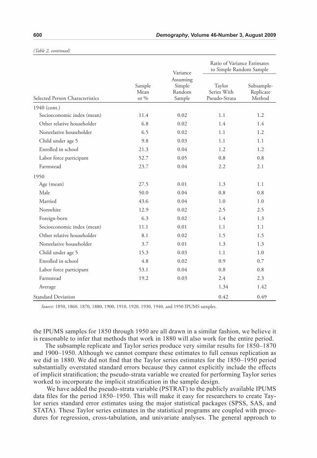
600 Demography, Volume 46-Number 3, August 2009
(Table 2, continued)
Ratio of Variance Estimates Variance to Simple Random Sample ____________________________ Assuming Sample Simple Taylor Subsample- Mean Random Series With ReplicateSelected Person Characteristics or % Sample Pseudo-Strata Method
1940 (cont.)Socioeconomic index (mean) 11.4 0.02 1.1 1.2 Other relative householder 6.8 0.02 1.4 1.4 Nonrelative householder 6.5 0.02 1.1 1.2 Child under age 5 9.8 0.03 1.1 1.1 Enrolled in school 21.3 0.04 1.2 1.2Labor force participant 52.7 0.05 0.8 0.8 Farmstead 23.7 0.04 2.2 2.1
1950Age (mean) 27.5 0.01 1.3 1.1 Male 50.0 0.04 0.8 0.8 Married 43.6 0.04 1.0 1.0 Nonwhite 12.9 0.02 2.5 2.5 Foreign-born 6.3 0.02 1.4 1.3 Socioeconomic index (mean) 11.1 0.01 1.1 1.1 Other relative householder 8.1 0.02 1.5 1.5 Nonrelative householder 3.7 0.01 1.3 1.3 Child under age 5 15.3 0.03 1.1 1.0 Enrolled in school 4.8 0.02 0.9 0.7 Labor force participant 53.1 0.04 0.8 0.8 Farmstead 19.2 0.03 2.4 2.3 Average 1.34 1.42
Standard Deviation 0.42 0.49
Source: 1850, 1860, 1870, 1880, 1900, 1910, 1920, 1930, 1940, and 1950 IPUMS samples.
the IPUMS samples for 1850 through 1950 are all drawn in a similar fashion, we believe it is reasonable to infer that methods that work in 1880 will also work for the entire period.
The subsample replicate and Taylor series produce very similar results for 1850–1870 and 1900–1950. Although we cannot compare these estimates to full census replication as we did in 1880. We did not fi nd that the Taylor series estimates for the 1850–1950 period substantially overstated standard errors because they cannot explicitly include the effects of implicit stratifi cation; the pseudo-strata variable we created for performing Taylor series worked to incorporate the implicit stratifi cation in the sample design.
We have added the pseudo-strata variable (PSTRAT) to the publicly available IPUMS data fi les for the period 1850–1950. This will make it easy for researchers to create Tay-lor series standard error estimates using the major statistical packages (SPSS, SAS, and STATA). These Taylor series estimates in the statistical programs are coupled with proce-dures for regression, cross-tabulation, and univariate analyses. The general approach to

Drawing Statistical Inferences From Historical Census Data 601
variance estimation discussed in this article is currently being tested on U.S. census data from 1940 to the present (which have a different sample design), and also on more than 200 non-U.S. census data from 75 countries.
The results presented here demonstrate that in certain circumstances, treating historical IPUMS data as simple random samples will yield underestimates of standard errors, and this could cause researchers to draw unwarranted statistical conclusions. The results also show, however, that for characteristics that are not highly correlated within clusters (i.e., households)—such as sex, socioeconomic index, or labor force participation—a simple random sample assumption can provide a reasonable estimate of standard errors.
Many analyses of IPUMS data do not pose standard error estimation problems. Recent IPUMS-based publications have focused, for example, on elderly persons residing with their adult children (Ruggles 2007), mothers of young children (Short, Goldscheider, and Torr 2006), men aged 20–39 (Rosenfeld 2006), and married couples in which the wife is aged 18–40 (Schwartz and Mare 2005). In each of these cases, the researchers examined a population subgroup that typically appears just once per household. For example, most households contain no more than one intergenerational coresident group, one mother of small children, one young adult man, or one young married couple. In such cases, there is little or no clustering and thus little reduction in statistical power. It follows that for most analyses, assuming a simple random sample will yield acceptable estimates of standard errors. Furthermore, regression models that have control variables related to sample design and clustering are less affected by the stratifi cation and clustering adjustments (e.g., see Davern et al. 2007; Kish and Frankel 1974).
There are some situations, however, in which the likelihood of large clustering effects is greater. Analyses of historical school attendance pose risk because if one child in a family attended school, the odds are high that all the school-age children were in school. Many schooling analyses, however, subdivide the schoolchildren by age and sex; such studies avoid clustering effects because a given household is unlikely to have multiple children of a particular age and sex. The worst clustering arises with analysis of popula-tion characteristics that almost by defi nition apply to entire households or families, such as poverty or urban residence. Even with these topics, however, the clustering problem evaporates if the unit of analysis does not usually occur more than once per household. Thus, for example, studies of the poverty status of families, householders, or mothers would be virtually unaffected by clustering.
In the end, researchers must evaluate their research designs and judge whether they pose a potential risk of clustering that might lead to underestimated standard errors. Where a signifi cant risk exists, we recommend that data users make use of the new strata and cluster variables on the IPUMS Web site to produce Taylor series standard error estimates using the statistical package of their choice. This methodology can be used both for calculating percentages and means (as it was in this article) and for calculating regres-sion models (e.g., ordinary least squares and logistic regression). These procedures will allow researchers to take advantage of implicit geographic stratifi cation while also paying attention to the clustering of people and their characteristics within sampled households. The subsample-replicate estimates were also found to produce reasonable standard error estimates and the subsample identifi ers are available in the IPUMS data fi les; but these estimates are harder to obtain because with this method, each analysis needs to be run 100 times, and standard errors must be calculated from the resulting sampling distribution.
APPENDIX A: DEMOGRAPHY ARTICLES THAT USED 1850–1950 MICRODATA FOR ORIGINAL ANALYSISAlba, R., J. Logan, A. Lutz, and B. Stults. 2002. “Only English by the Third Generation? Loss and
Preservation of the Mother Tongue Among the Grandchildren of Contemporary Immigrants.” Demography 39:467–84.
602 Demography, Volume 46-Number 3, August 2009
Elman, C. and G.C. Myers. 1999. “Geographic Morbidity Differentials in the Late Nineteenth-Century United States.” Demography 36:429–43.
Goldscheider, F.K. and R.M. Bures. 2003. “The Racial Crossover in Family Complexity in the United States.” Demography 40:569–87.
Gutmann, M.P., M.R. Haines, W.P. Frisbie, and K.S. Blanchard. 2000. “Intra-ethnic Diversity in Hispanic Child Mortality, 1890–1910.” Demography 37:467–75.
Hacker, J.D. 2003. “Rethinking the ‘Early’ Decline of Marital Fertility in the United States.” Demography 40:605–20.
Haines, M.R. and A.M. Guest. 2008. “Fertility in New York State in the Pre–Civil War Era.” Demography 45:345–61.
Hao, L. and Y. Kawano. 2001. “Immigrants’ Welfare Use and Opportunity for Contact With Co-ethnics.” Demography 38:375–89.
Hill, M.E. 1999. “Multivariate Survivorship Analysis Using Two Cross-Sectional Samples.” Demography 36:497–503.
Hirschman, C. 2005. “Immigration and the American Century.” Demography 42:595–620.Iceland, J. 2003. “Why Poverty Remains High: The Role of Income Growth, Economic Inequality,
and Changes in Family Structure, 1949–1999.” Demography 40:499–519. Kritz, M.M. and D.T. Gurak. 2001. “The Impact of Immigration on the Internal Migration of Natives
and Immigrants.” Demography 38:133–45.London, A.S. and C. Elman. 2001. “The Infl uence of Remarriage on the Racial Difference in Mother-
Only Families in 1910.” Demography 38:283–97. McGarry, K. and R.F. Schoeni. 2000. “Social Security, Economic Growth, and the Rise in Elderly
Widows’ Independence in the Twentieth Century.” Demography 37:221–36. Ruggles, S. 1997. “The Rise of Divorce and Separation in the United States, 1880–1990.”
Demography 34:455–66. Sassler, S. 1995. “Trade-Offs in the Family: Sibling Effects on Daughters’ Activities in 1910.”
Demography 32:557–75.Schoeni, R.F. 1998. “Reassessing the Decline in Parent-Child Old-Age Coresidence During the Twen-
tieth Century.” Demography 35:307–13. Schwartz, C.R. and R.D. Mare. 2005. “Trends in Educational Assortative Marriage From 1940 to
2003.” Demography 42:621–46. Short, S.E., F.K. Goldscheider, and B.M. Torr. 2006. “Less Help for Mother: The Decline in Coresi-
dential Female Support for the Mothers of Young Children, 1880–2000.” Demography 43:617–29.Stevens, G. 1999. “A Century of U.S. Censuses and the Language Characteristics of Immigrants.”
Demography 36:387–97.White, K.J.C. 2008. “Population Change and Farm Dependence: Temporal and Spatial Variation in
the U.S. Great Plains, 1900–2000.” Demography 45:363–86.White, K.J.C., K. Crowder, S.E. Tolnay, and R.M. Adelman. 2005. “Race, Gender, and Marriage:
Destination Selection During the Great Migration.” Demography 42:215–41.
REFERENCESDavern, M., A. Jones Jr., J. Lepkowski, G. Davidson, and L.A. Blewett. 2007. “Estimating Standard
Errors for Regression Coeffi cients Using the Current Population Survey’s Public Use File.” Inquiry 44:211–24.
Dippo, C.S. and K.M. Wolter. 1984. “A Comparison of Variance Estimators Using the Taylor Series Approximation.” Pp. 112–21 in ASA Proceedings of the Section on Survey Research Methods. Arlington, VA: American Statistical Association.
Goeken, R., C. Nguyen, S. Ruggles, and W.L. Sargent. 2003. “The 1880 United States Population Database.” Historical Methods 36(4):27–34.
Graubard, B.I. and E.L. Korn. 1996. “Survey Inference for Subpopulations.” American Journal of Epidemiology 144:102–106.

Drawing Statistical Inferences From Historical Census Data 603
Hammer, H., Hee-Choon Shin, and L.E. Porcellini. 2003. “A Comparison of Taylor Series and JK1 Resampling Methods for Variance Estimation.” Pp. 1–9 in Proceedings of the Hawaii Interna-tional Conference on Statistics. Honolulu, HI.
Hansen, M.H., W. Hurwitz, and W. Madow. 1953. Sample Survey Methods and Theory. New York: Wiley and Sons.
Kalton, G. 2002. “Model in the Practice of Survey Sampling (Revisited).” Journal of Offi cial Statis-tics 18:129–54.
Kish, L. 1965. Survey Sampling. New York: Wiley and Sons.———. 1992. “Weighting for Unequal Pi.” Journal of Offi cial Statistics 8:183–200.Kish, L. and M.R. Frankel. 1974. “Inference From Complex Samples.” Journal of the Royal Statisti-
cal Society Series B 36:1–37.Korn, E.L. and B.I. Graubard. 1995. “Examples of Differing Weighted and Unweighted Estimates
From a Sample Survey.” American Statistician 49:291–95.———. 1999. Analysis of Health Surveys. New York: Wiley.Krewski, D. and J.N.K. Rao. 1981. “Inference From Stratifi ed Samples: Properties of Linearization,
Jackknife and Balanced Repeated Replication Methods.” Annals of Statistics 9:1010–19.Little, R.J.A. 2003. “To Model or Not To Model? Competing Modes of Inference for Finite Popula-
tion Sampling.” The University of Michigan Department of Biostatistics Working Paper Series, Working Paper 4. Available online at http://www.bepress.com/umichbiostat/paper4.
Magnuson, D.L. 1995. “The Making of a Modern Census: The United States Census of Population, 1790–1940.” Ph.D. dissertation. Department of History, University of Minnesota.
Magnuson, D.L. and M.L. King. 1995. “Enumeration Procedures” Historical Methods 28:27–32.Rosenfeld, M.J. 2006. “Young Adulthood as a Factor in Social Change in the United States.” Popula-
tion and Development Review 43:617–29.Ruggles, S. 2007. “The Decline of Intergenerational Coresidence in the United States.” American
Sociological Review 72:962–89.Ruggles, S. and S. Brower. 2003. “The Measurement of Family and Household Composition in the
United States, 1850–1999.” Population and Development Review 29:73–101.Ruggles, S. and R.R. Menard. 1995. Public Use Microdata Sample of the 1880 United States Census
of Population: User’s Guide and Technical Documentation. Minneapolis: Social History Research Laboratory.
Ruggles, S., M. Sobek, T. Alexander, C.A. Fitch, R. Goeken, P.K. Hall, M. King, and C. Ron-nander. 2004. Integrated Public Use Microdata Series: Version 3.0 [Machine-readable database]. Minneapolis, MN: Minnesota Population Center [producer and distributor].
Rust, K. 1985. “Variance Estimation for Complex Estimators in Sample Surveys.” Journal of Offi cial Statistics 1:381–97.
SAS. 1999. Documentation for SAS Version 8. Cary, NC: SAS Institute, Inc.Schwartz, C.R. and R.D. Mare. 2005. “Trends in Educational Assortative Mating, 1940–2003.”
Demography 42:621–46.Short, S.E., F.K. Goldscheider, and B.M. Torr. 2006. “Less Help for Mother: The Decline in Co-
residential Female Support for the Mothers of Young Children, 1880–2000.” Demography 43:617–29.
SPSS. 2003. Correctly and Easily Compute Statistics for Complex Sampling. Chicago: SPSS Inc. Available online at http://www.spss.com/complex_samples.
Stata. 2001. Reference Manual. College Station, TX: STATA Press.Verma, V. 1993. Sampling Errors in Household Surveys. United Nations National Household Survey
Capability Programme. New York: U.N. Statistics Division, United Nations.Weng, S.S., F. Zhang, and M.P. Cohen. 1995. “Variance Estimates Comparison by Statistical Soft-
ware.” Pp. 333–38 in ASA Proceedings of the Section on Survey Research Methods. Arlington, VA: American Statistical Association.
Wolter, K.M. 1985. Introduction to Variance Estimation. New York: Springer-Verlag.