Drainage of Bank Storage in Shallow Unconfined Aquifers

5

Drainage of Bank Storage in Shallow Unconfined Aquifers

Abdelkader Djehiche1, Mustapha Gafsi1 and Konstantin Kotchev2 1LRGCU Amar Telidji, Laghouat,

2Ploytechnique, Sofia, 1Algeria

2Bulgaria

1. Introduction

The present work concerns subsurface drainage systems. The problems of surface and subsurface draining excess water from the canal or river are the major preoccupation of many researchers for at least 50 years; therefore we devoted this study to find appropriate solutions for problems encountered in the drainage of bank storage in shallow unconfined aquifers.

It is necessary to develop special processes such as the drains, the filters and to choose the type of the most effective drain to drain excess water from the canal. We have performed a study on a reduced model, of a homogeneous soil with trench drain on an impervious foundation, and we have proposed a correlation to determine the best position of the trench drain in the homogeneous soil. The water level in the trench drains can be directly determined for a given head of water in the canal, slope of the canal and the permeability coefficient, so that the seepage analysis is simplified to a certain degree and the accuracy is also satisfied based on the new approach. Finally comparative studies between experimental and numerical results using [SEEP] software were carried out.

2. Horizontal drainage

2.1 Steady and parallel flow in unconfined aquifers

In this section, we discuss the flow of groundwater to trench drains under steady state conditions. The steady-state theory is based on the assumption that the rate of recharge to the groundwater and evaporation is null.

Figure 1 shows a typical cross-section of a drainage system under this condition.

To describe the flow of groundwater to the trench drains, we have to make the following assumptions:

- Two-dimensional flow. This means that the flow is considered to be identical in any cross-section perpendicular to the drains; this is only true for infinitely long drains;

www.intechopen.com

Drainage Systems 90

- Homogeneous and isotropic soils with a permeability K. Thus we ignore any spatial variation in the hydraulic conductivity within a soil layer.

Most drainage equations are based on the Dupuit-Forchheimer assumptions (Ritzema, 1994):

Dupuit –Forchheimer equation:

懲態峙滴鉄岫朕岻鉄滴掴鉄 + 滴鉄岫朕岻鉄滴槻鉄峩 ± 圏 = ど (1)

Where q = recharge rate per unit area (m/ day /m2) and K = hydraulic conductivity of the soil (m/ day)

Fig. 1. Cross-sections of trench drains.

when q=0; This equation allows us to reduce the two-dimensional flow to a one-dimensional flow by assuming parallel and horizontal stream lines.

鳥鉄岫朕岻鉄鳥掴鉄 = ど (2)

Thus the solution of this equation is

ℎ態 = 系怠捲 + 系態 (3)

The limits conditions of this equation are

for x=0 h=H1

for x=E h=H2

where

H1 = elevation of the water level in the canal (m) H2 = elevation of the water level in the trench drain (m) E = drain spacing (m)

系怠 = 張迭鉄貸張鉄鉄帳 , 系態 = 茎怠態 (4)

y

x

H2

H1 h

QQ

E

q=0

K

www.intechopen.com

Drainage of Bank Storage in Shallow Unconfined Aquifers 91

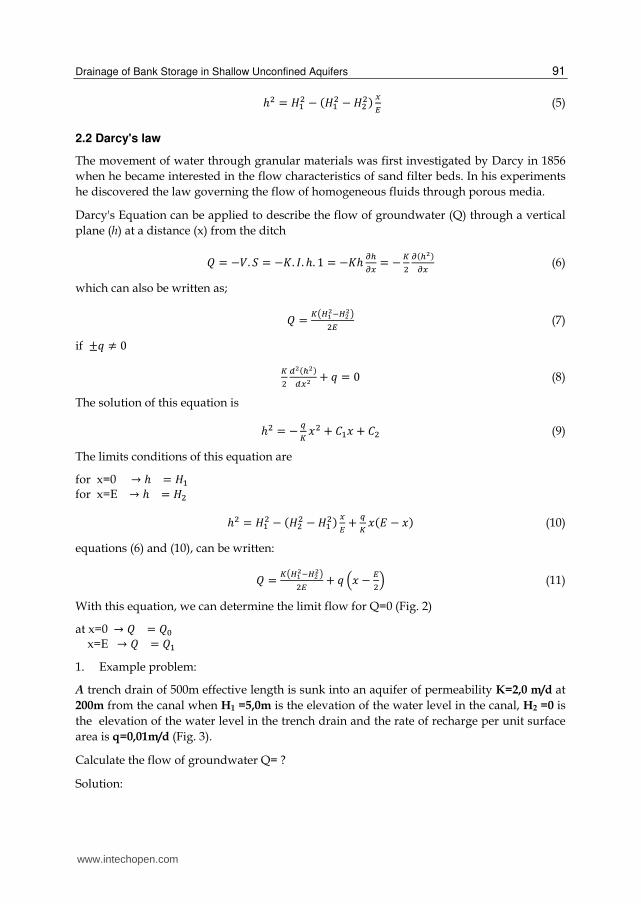
ℎ態 = 茎怠態 − 岫茎怠態 − 茎態態岻掴帳 (5)

2.2 Darcy's law

The movement of water through granular materials was first investigated by Darcy in 1856 when he became interested in the flow characteristics of sand filter beds. In his experiments he discovered the law governing the flow of homogeneous fluids through porous media.

Darcy's Equation can be applied to describe the flow of groundwater (Q) through a vertical plane (h) at a distance (x) from the ditch

芸 = −撃. 鯨 = −計. 荊. ℎ. な = −計ℎ 擢朕擢掴 = − 懲態擢岫朕鉄岻擢掴 (6)

which can also be written as;

芸 = 懲盤張迭鉄貸張鉄鉄匪態帳 (7)

if ±圏 ≠ ど

懲態鳥鉄岫朕鉄岻鳥掴鉄 + 圏 = ど (8)

The solution of this equation is

ℎ態 = − 槌懲捲態 + 系怠捲 + 系態 (9)

The limits conditions of this equation are

for x=0 → ℎ = 茎怠

for x=E → ℎ = 茎態

ℎ態 = 茎怠態 − 岫茎態態 − 茎怠態岻掴帳 + 槌懲捲岫継 − 捲岻 (10)

equations (6) and (10), can be written:

芸 = 懲盤張迭鉄貸張鉄鉄匪態帳 + 圏岾捲 − 帳態峇 (11)

With this equation, we can determine the limit flow for Q=0 (Fig. 2)

at x=0 → 芸 = 芸待 x=E → 芸 = 芸怠

1. Example problem:

A trench drain of 500m effective length is sunk into an aquifer of permeability K=2,0 m/d at 200m from the canal when H1 =5,0m is the elevation of the water level in the canal, H2 =0 is the elevation of the water level in the trench drain and the rate of recharge per unit surface area is q=0,01m/d (Fig. 3).

Calculate the flow of groundwater Q= ?

Solution:

www.intechopen.com

Drainage Systems 92

We are given:

H1=5,0m; H2=0; B=500m; K=2,0m/d; q=0,01m/d; E=200m.

Fig. 2. Cross-sections of open field drains, showing a curved watertable.

The flow of groundwater (Q) through a vertical plane (h) at a distance (x) from the ditch is given by this equation

芸 = 計岫茎怠態 − 茎態態岻に継 + 圏磐捲 − 継に卑

Numerical application:

a. x=0; → 芸待 = 態岫泰鉄貸待岻態.態待待 + ど,どな岾ど − 態待待態峇 = −ど,ぱばの陳典鳥.陳鎮 b. x=E; → 芸待 = 泰待替待待 + ど.どな岾にどど − 態待待態峇 = な,なにの陳典鳥.陳鎮 For the whole length B, we have: ∑ 芸 = 芸. 稽: ∑ 芸待 = −ど,ぱばの.のどど = −ねぬば,の陳典鳥 = −の,どは健/嫌

∑ 芸帳 = な,なにの.のどど = のはに,の陳典鳥 = は,のな健/嫌

2sec variant: when q=0

The discharge can be expressed by the following formula:

芸 = 計岫茎怠態 − 茎態態岻に継

Numerical application:

芸 = 態岫泰鉄貸待岻態.態待待 = ど,なにの陳典鳥.陳鎮;

H2

H1

Q0 Q1

E

q= 系剣券嫌建

K

Q=0

www.intechopen.com


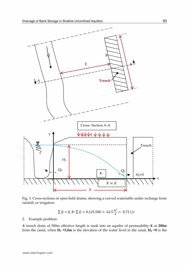
Fig. 3. Cross-sections of open field drains, showing a curved watertable under recharge from rainfall, or irrigation.

∑ 芸 = 芸. 稽: ∑ 芸 = ど,なにの.のどど = はに.の陳典鳥 = ど,ばに健/嫌

2. Example problem:

A trench drain of 500m effective length is sunk into an aquifer of permeability K at 200m from the canal, when H1 =5,0m is the elevation of the water level in the canal, H2 =0 is the

K

Q B E A

A Trench

y

x H2=0

H1

Q0 QE

E

q

計寐 ≪ 計

Cross- Section A-A

Trench

www.intechopen.com

Drainage Systems 94

elevation of the water level in the trench drain, the rate of recharge per unit surface area is

q=0,01m/d and the flow of groundwater is ∑ 芸 = などど陳典鳥

Calculate the permeability of the aquifer K = ?

Solution: We are given:

H1=5,0m ; H2=0 ; B=500m ; q=0,01m/d ; E=200m; ∑ 芸 = 芸. 稽 = などど陳典鳥 .

the permeability of the aquifer K is: 計 = 態町帳岫張迭鉄貸張鉄鉄岻 = 態.待,態待待.態待待岫泰鉄貸待岻 = 腿待態泰 = ぬ,に陳典鳥 ;

the flow of groundwater Q: 芸 = ∑ 町喋 = 怠待待泰待待 = ど,に陳典鳥.陳鎮 2.3 Grapho-Analytical Method for parallel drainage

The pumping rate is estimated by the formula of Chapman (Leonards, 1968)

圏 = 懲追岫茎 − ど,にばℎ待岻岫茎態 − ℎ待態岻 (12)

Fig. 4. Flow of groundwater to subsurface drains in shallow unconfined aquifers.

The following equation can be used to determine the elevation of the watertable midway between the drains:

ℎ鳥 = ℎ待峙寵迭寵鉄追岫茎 − ℎ待岻 + な峩 (13)

www.intechopen.com


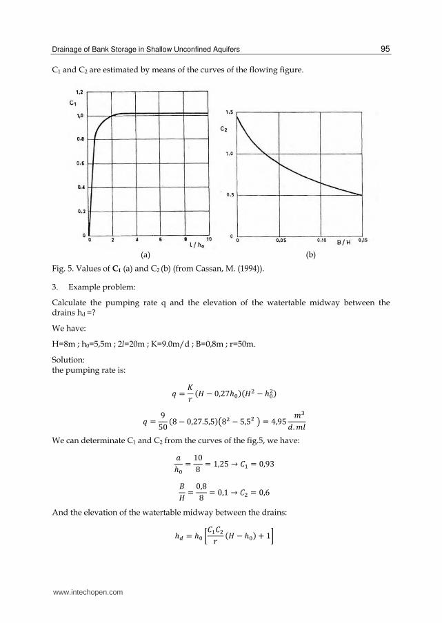
C1 and C2 are estimated by means of the curves of the flowing figure.

(a) (b)

Fig. 5. Values of C1 (a) and C2 (b) (from Cassan, M. (1994)).

3. Example problem:

Calculate the pumping rate q and the elevation of the watertable midway between the drains hd =?

We have:

H=8m ; h0=5,5m ; 2l=20m ; K=9.0m/d ; B=0,8m ; r=50m.

Solution: the pumping rate is:

圏 = 計堅岫茎 − ど,にばℎ待岻岫茎態 − ℎ待態岻

圏 = ひのど岫ぱ − ど,にば.の,の岻盤ぱ態 − の,の態匪 = ね,ひの兼戴穴. 兼健 We can determinate C1 and C2 from the curves of the fig.5, we have: 欠ℎ待 = などぱ = な,にの → 系怠 = ど,ひぬ稽茎 = ど,ぱぱ = ど,な → 系態 = ど,は

And the elevation of the watertable midway between the drains:

ℎ鳥 = ℎ待釆系怠系態堅岫茎 − ℎ待岻 + な挽

www.intechopen.com

Drainage Systems 96

ℎ鳥 = の,の釆ど,ひぬ.ど,はのど岫ぱ − の,の岻 + な挽 = の,はの兼

The drawdown of water level is: 茎 − ℎ鳥 = ぱ − の,はの = に,ぬの兼

3. Single horizontal drainage in unconfined aquifers

3.1 Perfect drainage

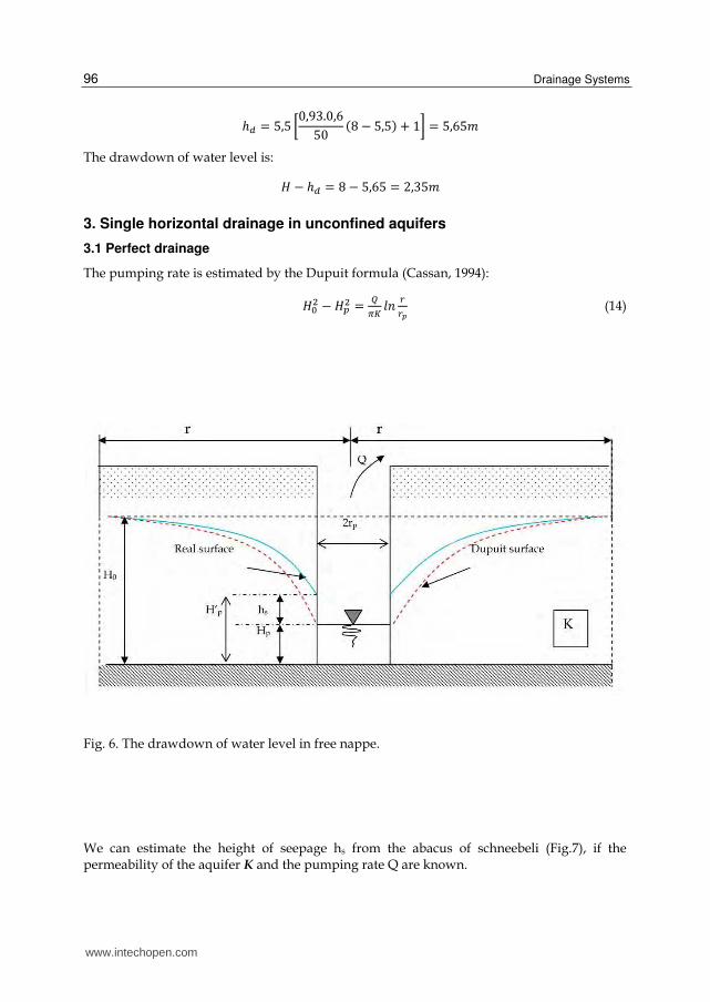
The pumping rate is estimated by the Dupuit formula (Cassan, 1994):

茎待態 − 茎椎態 = 町訂懲健券追追妊 (14)

Fig. 6. The drawdown of water level in free nappe.

We can estimate the height of seepage hs from the abacus of schneebeli (Fig.7), if the permeability of the aquifer K and the pumping rate Q are known.

www.intechopen.com


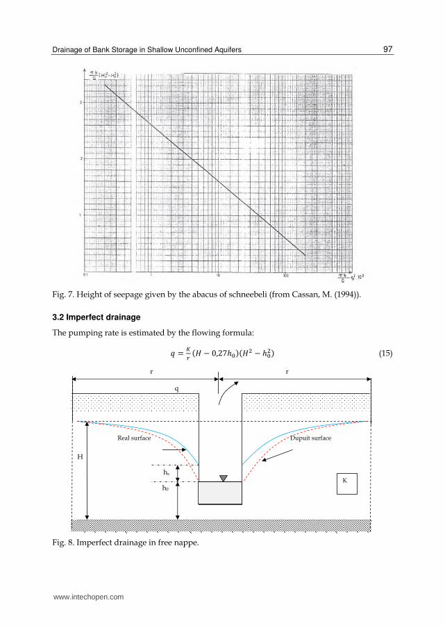
Fig. 7. Height of seepage given by the abacus of schneebeli (from Cassan, M. (1994)).

3.2 Imperfect drainage

The pumping rate is estimated by the flowing formula:

圏 = 懲追岫茎 − ど,にばℎ待岻岫茎態 − ℎ待態岻 (15)

Fig. 8. Imperfect drainage in free nappe.

www.intechopen.com

Drainage Systems 98

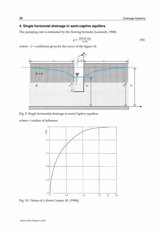
4. Single horizontal drainage in semi-captive aquifers

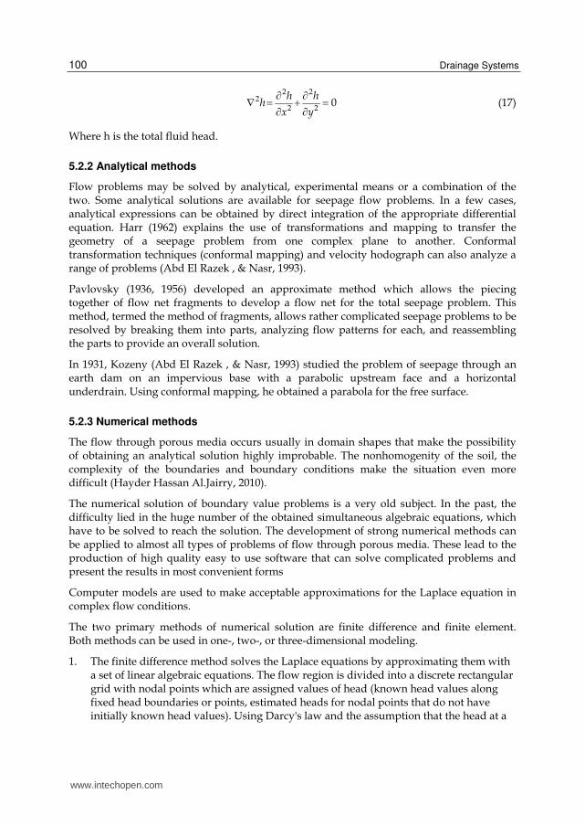
The pumping rate is estimated by the flowing formula (Leonards, 1968):

圏 = 態懲帖岫張貸朕轍岻鎮袋碇帖 (16)

where: 膏 = coefficient given by the curve of the figure 10.

Fig. 9. Single horizontal drainage in semi-Captive aquifers.

where r =radius of influence

Fig. 10. Values of 膏 (from Cassan, M. (1994)).

www.intechopen.com


5. Drainage of bank storage in shallow unconfined aquifers

5.1 Shallow unconfined aquifers

Unconfined aquifers are associated with the presence of a free water table, therefore the groundwater can flow in any direction: horizontal, vertical, or intermediate between them. Shallow unconfined aquifers have a shallow impermeable layer (say at 0.5 to 2 m below the soil surface). The flow of groundwater to subsurface drains above a shallow impermeable layer is mainly horizontal and occurs mostly above drain level (Fig. 11). In shallow unconfined aquifers, it is usually sufficient to measure the horizontal hydraulic conductivity of the soil above drain level (i.e. Ka). The recharge of water to a shallow aquifer occurs only as the percolation of rain or irrigation water; there is neither upward seepage of groundwater nor any natural drainage. Since the transmissivity of a shallow aquifer is small, the horizontal flow in the absence of subsurface drains is usually neglected (from Oosterbaan, R.J. & Nijland, H.J. (1994)).

Fig. 11. Flow of groundwater to subsurface drains in shallow unconfined aquifers (from Oosterbaan, R.J. & Nijland, H.J. (1994)).

5.2 Methods for solving unconfined drainage

5.2.1 Introduction

A large number of procedures have been used to solve seepage problems through porous medium, graphical, analytical, experimental and numerical methods were introduced in literatures to determine the hydraulic parameters of seepage through homogeneous soil.

The governing steady flow which can be described by the Laplace equation (Equation 17) is developed from application of the law of mass conservation with Darcy’s Law can be solved by a graphical construction of a flow net. A flow net is a network of curves called streamlines and equipotential lines. A streamline is an imaginary line that traces the path that a particle of groundwater would follow as it flows through an aquifer. In an isotropic aquifer, streamlines are perpendicular to equipotential lines.

For isotropic soil the Laplace equation is:

www.intechopen.com

Drainage Systems 100

2 2

22 2 0h h

hx y

(17)

Where h is the total fluid head.

5.2.2 Analytical methods

Flow problems may be solved by analytical, experimental means or a combination of the two. Some analytical solutions are available for seepage flow problems. In a few cases, analytical expressions can be obtained by direct integration of the appropriate differential equation. Harr (1962) explains the use of transformations and mapping to transfer the geometry of a seepage problem from one complex plane to another. Conformal transformation techniques (conformal mapping) and velocity hodograph can also analyze a range of problems (Abd El Razek , & Nasr, 1993).

Pavlovsky (1936, 1956) developed an approximate method which allows the piecing together of flow net fragments to develop a flow net for the total seepage problem. This method, termed the method of fragments, allows rather complicated seepage problems to be resolved by breaking them into parts, analyzing flow patterns for each, and reassembling the parts to provide an overall solution.

In 1931, Kozeny (Abd El Razek , & Nasr, 1993) studied the problem of seepage through an earth dam on an impervious base with a parabolic upstream face and a horizontal underdrain. Using conformal mapping, he obtained a parabola for the free surface.

5.2.3 Numerical methods

The flow through porous media occurs usually in domain shapes that make the possibility of obtaining an analytical solution highly improbable. The nonhomogenity of the soil, the complexity of the boundaries and boundary conditions make the situation even more difficult (Hayder Hassan Al.Jairry, 2010).

The numerical solution of boundary value problems is a very old subject. In the past, the difficulty lied in the huge number of the obtained simultaneous algebraic equations, which have to be solved to reach the solution. The development of strong numerical methods can be applied to almost all types of problems of flow through porous media. These lead to the production of high quality easy to use software that can solve complicated problems and present the results in most convenient forms

Computer models are used to make acceptable approximations for the Laplace equation in complex flow conditions.

The two primary methods of numerical solution are finite difference and finite element. Both methods can be used in one-, two-, or three-dimensional modeling.

1. The finite difference method solves the Laplace equations by approximating them with a set of linear algebraic equations. The flow region is divided into a discrete rectangular grid with nodal points which are assigned values of head (known head values along fixed head boundaries or points, estimated heads for nodal points that do not have initially known head values). Using Darcy's law and the assumption that the head at a

www.intechopen.com


given node is the average of the surrounding nodes, a set of N linear algebraic equations with N unknown values of head are developed (N equals number of nodes). Normally, N is large and relaxation methods involving iterations and the use of a computer must be applied.

2. The finite element method is a second way of numerical solution.

This method is also based on grid pattern (not necessarily rectangular) which divides the flow region into discrete elements and provides N equations with N unknowns. Material properties, such as permeability, are specified for each element and boundary conditions (heads and flow rates) are set. A system of equations is solved to compute heads at nodes and flows in the elements.

The finite element has several advantages over the finite difference method for more complex seepage problems. These include (Radhakrishnan, 1978):

a. Complex geometry including sloping layers of material can be easily accommodated. b. By varying the size of elements, zones where seepage gradients or velocity are high can

be accurately modeled. c. Pockets of material in a layer can be modeled.

5.2.4 Graphical method

The graphical method can be used to solve a wider class of problems than analytical method. Its advantage is highly remarkable in case of potential flow through domains with irregular boundaries. Other types of flow such as through two dimensional anisotropic homogeneous soil or multilayers can also be treated graphically.

Flow nets are one of the most useful and accepted methods for solution of Laplace's equation (Casagrande, 1937). If boundary conditions and geometry of a flow region are known and can be displayed two dimensionally, a flow net can provide a strong visual sense of what is happening (pressures and flow quantities) in the flow region.

To draw the flow net, the following conditions are to be satisfied as follows (Harry, 1989);

1. all impermeable boundaries are streamlines, 2. all water bodies are lines of constant head (equipotential lines), 3. streamlines meet equipotential lines at right angles, 4. streamlines do not intersect one another, and

5. equipotential lines do not intersect one another.

Using the previous conditions, it is recommended to start the flow net construction by drawing the streamlines taking the advantage of the existing impermeable surfaces in the domain of flow and making sure that they meet water bodies at right angles. However, the graphical method requires a lot of experience and many trial and error works before reaching a solution with reasonable accuracy.

5.2.5 Experimental model

Experimental methods are considered useful for simulating the flow of water by models in laboratory. There are two types of models, electrical model, which analogous the flow of

www.intechopen.com


water by a flow of current and physical models such as sandbox model and viscous flow model (Hele-Shaw model). These methods have some inconvenient such as the complicated construction and operation. In Hele-Shaw model, the viscosity of the fluid varies with temperature, and sandbox model suffers from the difficulty of representing the correct permeability of the soil and because of the difficulties caused by capillarity. In this study we have used a sandbox model.

5.2.5.1 Sand-box model

Sand models which may use prototype materials can provide information about flow paths and head at particular points in the aquifer. We have constructed a scale model (generally sand) of the prototype in a sandbox equipped from perforated front and which allow the passage of water. When steady-state flow is reached, the flow can be traced by dye injection at various points along the upstream boundary close to the transparent wall to form the traces of streamlines, and heads determined by small piezometers (El-Masry, 1995; Khalaf Allah, 2005).

A small-scale model was built; which is geometrically similar to the real system. This model represents a homogeneous soil (bank storage in shallow unconfined aquifers) with a trench drain on an impervious foundation. Sand has been used as a permeable medium for the body of the soil, provided that its permeability is such as the flow remains laminar and that there is not any effect of distortion by capillarity (the grains should not be lower than 0,7 mm) (Mallet & Pacouant, 1951) and of gravel for the trench drain. The piezometric prickings laid out on the two zones with dimensions of the tank make it possible to know the actual values of the head of water along the trajectory of flow and highlight the burden-sharing of water in the seepages (Bear, 1972; Casagrande, 1973; Harr, 1962).

6. Reduced model of bank storage in shallow unconfined aquifers

6.1 Determination of the material characteristics

The characteristics of materials used in this model have been determined (sand for the soil and gravel for the drain) such as the vertical and horizontal permeability

6.2 Vertical permeability

It is given according to the Darcy’ law:

芸 = 計塚. 鯨荊 (18)

where Q = quantity of discharge; S = cross-sectional area of flow; I = hydraulic gradient; Kv

= coefficient of vertical permeability.

We obtain,計塚= 4.9(m/day) = 5, 67.10-5 (m/s),

6.3 Horizontal permeability

This permeability is given according to the formula of Dupuit:

芸 = 懲廿盤張迭鉄貸張鉄鉄匪態挑 (19)

www.intechopen.com


where Q = quantity of discharge; H1 = the head of water upstream; H2 = the head of water downstream; L = the length of the sample; b = the width of the sample; Kh = coefficient of horizontal permeability. We obtain Kh= 43.2 (m/day) = 5.10-4(m/s).

7. Trench drain

7.1 Position of the trench drain

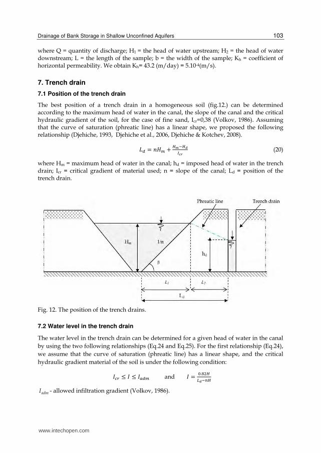
The best position of a trench drain in a homogeneous soil (fig.12.) can be determined according to the maximum head of water in the canal, the slope of the canal and the critical hydraulic gradient of the soil, for the case of fine sand, Icr=0,38 (Volkov, 1986). Assuming that the curve of saturation (phreatic line) has a linear shape, we proposed the following relationship (Djehiche, 1993, Djehiche et al., 2006, Djehiche & Kotchev, 2008).

詣鳥 = 券茎陳 + 張尿貸張匂彫迩認 (20)

where Hm = maximum head of water in the canal; hd = imposed head of water in the trench drain; Icr = critical gradient of material used; n = slope of the canal; Ld = position of the trench drain.

Fig. 12. The position of the trench drains.

7.2 Water level in the trench drain

The water level in the trench drain can be determined for a given head of water in the canal by using the two following relationships (Eq.24 and Eq.25). For the first relationship (Eq.24), we assume that the curve of saturation (phreatic line) has a linear shape, and the critical hydraulic gradient material of the soil is under the following condition:

荊頂追 ≤ 荊 ≤ 荊銚鳥陳 and 荊 = 待.腿態張挑匂貸津張

admI - allowed infiltration gradient (Volkov, 1986).

www.intechopen.com


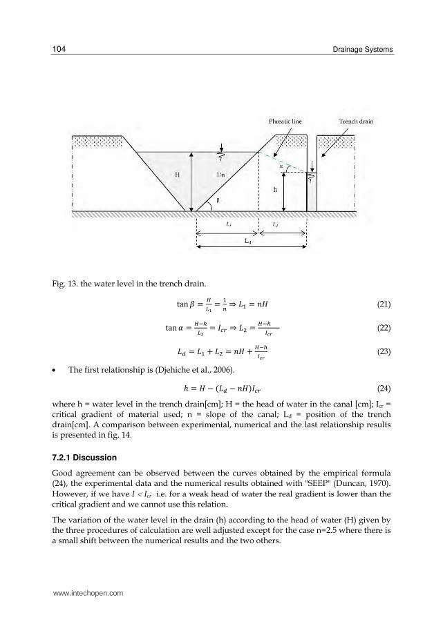
Fig. 13. the water level in the trench drain.

tan 紅 = 張挑迭 = 怠津 ⇒ 詣怠 = 券茎 (21)

tan 糠 = 張貸朕挑鉄 = 荊頂追 ⇒ 詣態 = 張貸朕��彫迩認 (22)

詣鳥 = 詣怠 + 詣態 = 券茎 + 張貸朕彫迩認 (23)

The first relationship is (Djehiche et al., 2006).

ℎ = 茎 − 岫詣鳥 − 券茎岻荊頂追 (24)

where h = water level in the trench drain[cm]; H = the head of water in the canal [cm]; Icr = critical gradient of material used; n = slope of the canal; Ld = position of the trench drain[cm]. A comparison between experimental, numerical and the last relationship results is presented in fig. 14.

7.2.1 Discussion

Good agreement can be observed between the curves obtained by the empirical formula (24), the experimental data and the numerical results obtained with "SEEP" (Duncan, 1970). However, if we have I Icr i.e. for a weak head of water the real gradient is lower than the critical gradient and we cannot use this relation.

The variation of the water level in the drain (h) according to the head of water (H) given by the three procedures of calculation are well adjusted except for the case n=2.5 where there is a small shift between the numerical results and the two others.

www.intechopen.com


(a) n=3,0

(b) n=2,5

0

2

4

6

8

10

12

14

16

18

14 19 24 29

h(c

m)

H(cm)

0

2

4

6

8

10

12

14

16

14 19 24 29

h(c

m)

H(cm)

www.intechopen.com


(c) n=2,0

Fig. 14. The lozenge represent the experimental results of the tests, the square represents the results obtained with equation (24), and the triangle represents the numerical results.

The second relationship under the following condition:

の ≤ 計朕計塚 ≤ ぬど

ℎ = 結琴欽欽欽欣轍.迭添店纏迭那磐凪廿凪寧卑轍.典

√韮貸典.典迭添迭俵凪廿凪寧韮迭.鉄筋禽禽禽禁 (25)

where h = water level in the trench drain[cm]; H = the head of water in the canal [cm]; Kh = coefficient of horizontal permeability; Kv = coefficient of vertical permeability; n = slope of the canal.

The comparison of results of this relationship with the results of SEEP (Duncan, 1970) "software" and the experimental results is represented in fig. 15.

0

2

4

6

8

10

12

14 19 24 29

h(c

m)

H(cm)

www.intechopen.com


(a)

(b)

0

2

4

6

8

10

12

14

16

18

14 19 24 29

h(cm)

H(cm)

n=3,0

0

2

4

6

8

10

12

14

16

14 19 24 29

h(cm)

H(cm)

n=2,5

www.intechopen.com


(c)

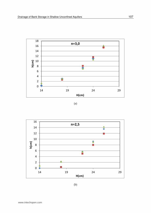
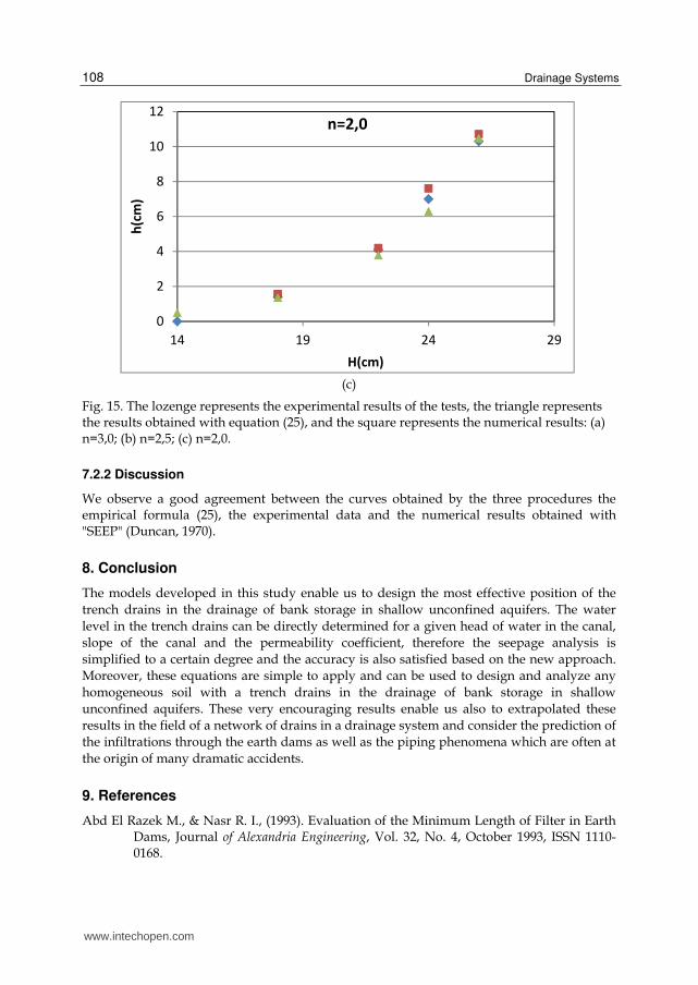
Fig. 15. The lozenge represents the experimental results of the tests, the triangle represents the results obtained with equation (25), and the square represents the numerical results: (a) n=3,0; (b) n=2,5; (c) n=2,0.

7.2.2 Discussion

We observe a good agreement between the curves obtained by the three procedures the empirical formula (25), the experimental data and the numerical results obtained with "SEEP" (Duncan, 1970).

8. Conclusion

The models developed in this study enable us to design the most effective position of the trench drains in the drainage of bank storage in shallow unconfined aquifers. The water level in the trench drains can be directly determined for a given head of water in the canal, slope of the canal and the permeability coefficient, therefore the seepage analysis is simplified to a certain degree and the accuracy is also satisfied based on the new approach. Moreover, these equations are simple to apply and can be used to design and analyze any homogeneous soil with a trench drains in the drainage of bank storage in shallow unconfined aquifers. These very encouraging results enable us also to extrapolated these results in the field of a network of drains in a drainage system and consider the prediction of the infiltrations through the earth dams as well as the piping phenomena which are often at the origin of many dramatic accidents.

9. References

Abd El Razek M., & Nasr R. I., (1993). Evaluation of the Minimum Length of Filter in Earth Dams, Journal of Alexandria Engineering, Vol. 32, No. 4, October 1993, ISSN 1110-0168.

0

2

4

6

8

10

12

14 19 24 29

h(cm)

H(cm)

n=2,0

www.intechopen.com


Bear, J.; (1972). Dynamics of Fluids in Porous Media, Elsevier, ISBN 0-444-00114-X, New York Casagrande,A. (1973). Seepage control in earth dams. J. Wiley & Sone. Chu , J.; Bo, M. W.; & Choa, V. (2004). Practical considerations for using vertical drains in

soil improvement projects, Geotextiles and Geomembranes , N° 22: pp 101–117, ISSN 0266-1144

Djehiche, A. (1993). Comportement des barrages en terre avec cheminée filtrante sous l’action de l’infiltration. Thèse Magister, Algeria: USTO, pp 121 (in Arabic).

Djehiche, A.; Derriche, Z. & Kotchev, K. (2006). Control of water head in the vertical drain. Proceedings of Dams and Reservoirs, Societies and Environment in the 21st Century, Vol.1, pp 913-916, ISBN-10: 0-415-40423-1.

Djehiche, A.; & Kotchev, K.; (2008). Control of seepage in earth dams with a vertical drain. Chinese Journal of Geotechnical Engineering, pp 1657-1660, Vol.30, Nov (2008), ISSN 1000-4548.

Duncan, J. M. (1970). SEEP, A computer for seepage with a free surface or confined steady flow. University of California: Berkeley.

Dunglas, J. & Loudiere, D. (1973). Nouvelle conception des drains dans les barrages en terre homogènes de petite et moyenne dimensions. La Houille Blanche, 5(6): pp. 461-465, ISSN 0018-6368.

El-Masry A. A., (1995). Unconfined Seepage through Earth Dams with Chimney Drain by Boundary Element Method”, Proceeding of First Engineering conference, Mansoura, March 1995, Vol. III. pp. 357-365.

Harr, M. E.; (1962). Groundwater and Seepage, McGraw-Hill Book Company, ISBN 0-486-66881-9, New York.

Harry R. Cedergren, (1989). Seepage, drainage, and flow nets. John Wiley & Sons, Inc., New York, NY.

Hayder Hassan Al.Jairry (2010) 2D-Flow Analysis Through Zoned Earth Dam Using Finite Element Approach, Eng. & Tech. Journal ,Vol.28, No.21,

Kahlown M. A. & Khan A.D. (2004). Tile drainage manual. Khyaban-e-Johar, H-8/1, Islamabad – Pakistan ISBN 969-8469-13-3

Khalaf Allah S., (2005). Seepage through Earth dams with Filters, M. Sc thesis, Dept. of Irrigation and Hydraulics Eng. Mansoura university , Egypt.

Leonards, G.A., (1968), Les Fondations (traduction de "Foundation Engineering". McGraw- Hill New York 1962 par un groupe d'ingénieurs des Laboratoires des Ponts et Chaussées). Dunod, Paris, 1106 p

Loudiere, D. (1972). Elément théorique sur le drainage dans les barrages en terre homogènes. C.T.G.R.E.F., Nov,

Mallet, Ch. & Pacouant, J. ; (1951). Les barrages en terre. Edition Eyrolles. Oosterbaan, R.J. & Nijland, H.J. (1994). Determining the saturated hydraulic conductivity.

Drainage Principles and Applications. International Institute for Land Reclamation and Improvement ( ILRI), Chapter 12 in: H.P.Ritzema (Ed.) Publication 16, second revised edition, Wageningen, The Netherlands. ISBN 90 70754 3 39

Ritzema, H.P. ; (1994). Subsurface Flow to Drains. Drainage Principles and Applications. International Institute for Land Reclamation and Improvement ( ILRI), Chapter 8 in: Publication 16, second revised edition, Wageningen, The Netherlands. ISBN 90 70754 3 39

www.intechopen.com


Thieu N.T. M., Fredlund D. G., Fredlund M. D. & Hung V. Q. (2001). Seepage Modeling in a saturated/unsaturated Soil System. International Conference on Management of the Land and Water Resources, MLWR, October 20-22, Hanoi, Vietnam.

Cassan, M. (1994). Aide-Memoire D'hydraulique Souterraine. Presses de l'école nationale des Ponts et Chaussées (ENPC) - 2ème Édition, France. ISBN-10: 2-85978-208-7

Volkov, V. (1986). Ouvrages hydrauliques. Guide de Thèse, ENSH, Blida, Algeria, pp 120-128. Xu Y.-Q., Unami K. & Kawachi T. (2003). Optimal hydraulic design of earth dam cross

section using saturated–unsaturated seepage flow model, Advances in Water Resources, 26: pp 1–7

Zhang J., Xu Q. & Chen Z.,( 2001). Seepage Analysis Based on the Unified Unsaturated Soil Theory, Mechanics Research Communications, , 28, No 1:pp 107-112,

www.intechopen.com

Drainage SystemsEdited by Prof. Muhammad Salik Javaid

ISBN 978-953-51-0243-4Hard cover, 240 pagesPublisher InTechPublished online 07, March, 2012Published in print edition March, 2012

InTech EuropeUniversity Campus STeP Ri Slavka Krautzeka 83/A 51000 Rijeka, Croatia Phone: +385 (51) 770 447 Fax: +385 (51) 686 166www.intechopen.com

InTech ChinaUnit 405, Office Block, Hotel Equatorial Shanghai No.65, Yan An Road (West), Shanghai, 200040, China

Phone: +86-21-62489820 Fax: +86-21-62489821

The subject of 'drainage: draining the water off' is as important as 'irrigation: application of water', if not more.'Drainage' has a deep impact on food security, agricultural activity, hygiene and sanitation, municipal usage,land reclamation and usage, flood and debris flow control, hydrological disaster management, ecological andenvironmental balance, and water resource management. 'Drainage Systems' provides the reader with a tri-dimensional expose of drainage in terms of sustainable systems, surface drainage and subsurface drainage.Ten eminent authors and their colleagues with varied technical backgrounds and experiences from around theworld have dealt with extensive range of issues concerning the drainage phenomenon. Field engineers,hydrologists, academics and graduate students will find this book equally benefitting.

How to referenceIn order to correctly reference this scholarly work, feel free to copy and paste the following:

Djehiche Abdelkader, Gafsi Mustapha and Kotchev Konstantin (2012). Drainage of Bank Storage in ShallowUnconfined Aquifers, Drainage Systems, Prof. Muhammad Salik Javaid (Ed.), ISBN: 978-953-51-0243-4,InTech, Available from: http://www.intechopen.com/books/drainage-systems/drainage-of-bank-storage-in-shallow-unconfined-aquifers

© 2012 The Author(s). Licensee IntechOpen. This is an open access articledistributed under the terms of the Creative Commons Attribution 3.0License, which permits unrestricted use, distribution, and reproduction inany medium, provided the original work is properly cited.

http://creativecommons.org/licenses/by/3.0

Documents

Drainage of Bank Storage in Shallow Unconfined Aquifers