DRAG SLED AND AUTOMOBILE SKIDDING; AN ... George Research 2008...DRAG SLED AND AUTOMOBILE SKIDDING; AN ANALYTICAL RELATIONSHIP by Frank Navin, Ph.D., D.Sc.(Hon), P.Eng Professor Emeritus

DRAG SLED AND AUTOMOBILE

SKIDDING; AN ANALYTICAL RELATIONSHIP

by Frank Navin, Ph.D., D.Sc.(Hon), P.Eng

Professor Emeritus Civil Engineering,

University of British Columbia

President, SYNECTICS RSR Corp. Vancouver, BC.

CANADA

for Institute for Police Technology and Management

University of North Florida Jacksonville, Florida,

USA

SPECIAL PROBLEMS 2009 Orlando, Florida

APRIL 2009

Drag Sled and Skidding Vehicles IPTM Special Problems 2009

DRAG SLED AND AUTOMOBILE SKIDDING;

AN ANALYTICAL RELATIONSHIP

Frank Navin, Ph.D., D.Sc.(Hon), P.Eng Professor Emeritus Civil Engineering, UBC

President, SYNECTICS RSR Corp.

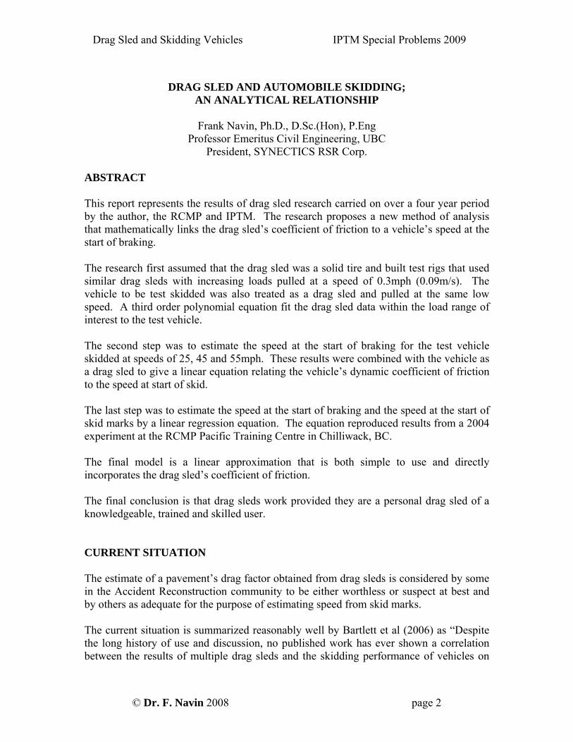
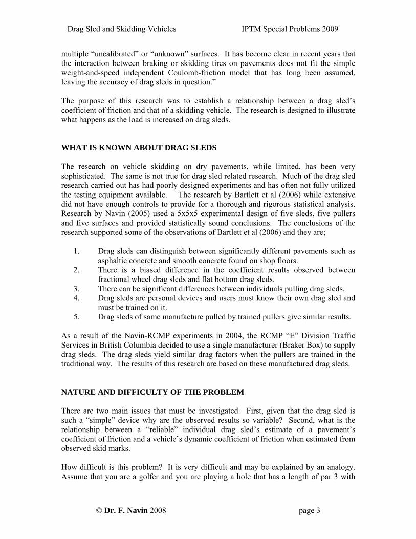
ABSTRACT This report represents the results of drag sled research carried on over a four year period by the author, the RCMP and IPTM. The research proposes a new method of analysis that mathematically links the drag sled’s coefficient of friction to a vehicle’s speed at the start of braking. The research first assumed that the drag sled was a solid tire and built test rigs that used similar drag sleds with increasing loads pulled at a speed of 0.3mph (0.09m/s). The vehicle to be test skidded was also treated as a drag sled and pulled at the same low speed. A third order polynomial equation fit the drag sled data within the load range of interest to the test vehicle. The second step was to estimate the speed at the start of braking for the test vehicle skidded at speeds of 25, 45 and 55mph. These results were combined with the vehicle as a drag sled to give a linear equation relating the vehicle’s dynamic coefficient of friction to the speed at start of skid. The last step was to estimate the speed at the start of braking and the speed at the start of skid marks by a linear regression equation. The equation reproduced results from a 2004 experiment at the RCMP Pacific Training Centre in Chilliwack, BC. The final model is a linear approximation that is both simple to use and directly incorporates the drag sled’s coefficient of friction. The final conclusion is that drag sleds work provided they are a personal drag sled of a knowledgeable, trained and skilled user. CURRENT SITUATION The estimate of a pavement’s drag factor obtained from drag sleds is considered by some in the Accident Reconstruction community to be either worthless or suspect at best and by others as adequate for the purpose of estimating speed from skid marks. The current situation is summarized reasonably well by Bartlett et al (2006) as “Despite the long history of use and discussion, no published work has ever shown a correlation between the results of multiple drag sleds and the skidding performance of vehicles on

© Dr. F. Navin 2008 page 2


multiple “uncalibrated” or “unknown” surfaces. It has become clear in recent years that the interaction between braking or skidding tires on pavements does not fit the simple weight-and-speed independent Coulomb-friction model that has long been assumed, leaving the accuracy of drag sleds in question.” The purpose of this research was to establish a relationship between a drag sled’s coefficient of friction and that of a skidding vehicle. The research is designed to illustrate what happens as the load is increased on drag sleds. WHAT IS KNOWN ABOUT DRAG SLEDS The research on vehicle skidding on dry pavements, while limited, has been very sophisticated. The same is not true for drag sled related research. Much of the drag sled research carried out has had poorly designed experiments and has often not fully utilized the testing equipment available. The research by Bartlett et al (2006) while extensive did not have enough controls to provide for a thorough and rigorous statistical analysis. Research by Navin (2005) used a 5x5x5 experimental design of five sleds, five pullers and five surfaces and provided statistically sound conclusions. The conclusions of the research supported some of the observations of Bartlett et al (2006) and they are;

1. Drag sleds can distinguish between significantly different pavements such as asphaltic concrete and smooth concrete found on shop floors.

2. There is a biased difference in the coefficient results observed between fractional wheel drag sleds and flat bottom drag sleds.

3. There can be significant differences between individuals pulling drag sleds. 4. Drag sleds are personal devices and users must know their own drag sled and

must be trained on it. 5. Drag sleds of same manufacture pulled by trained pullers give similar results.

As a result of the Navin-RCMP experiments in 2004, the RCMP “E” Division Traffic Services in British Columbia decided to use a single manufacturer (Braker Box) to supply drag sleds. The drag sleds yield similar drag factors when the pullers are trained in the traditional way. The results of this research are based on these manufactured drag sleds. NATURE AND DIFFICULTY OF THE PROBLEM There are two main issues that must be investigated. First, given that the drag sled is such a “simple” device why are the observed results so variable? Second, what is the relationship between a “reliable” individual drag sled’s estimate of a pavement’s coefficient of friction and a vehicle’s dynamic coefficient of friction when estimated from observed skid marks. How difficult is this problem? It is very difficult and may be explained by an analogy. Assume that you are a golfer and you are playing a hole that has a length of par 3 with



some complications. First, there is a sharp angle dog leg to the right half way to the hole. The hole is also obscured by trees and elevated above the tee-box. Second, your caddie keeps giving you new and different homemade clubs, the greens keepers are constantly moving the hole and finally there are random gusts of wind. Your performance is measured on how close you can come to the hole on the green. (This analogy comes in part from Tiger Woods memorable and winning shot on the 16th hole at the 2000 Canadian Open held at Glen Abbey Golf Course.) The solution to this problem requires “regular golfers” to abandon traditional methods and adopt a new approach. NEW APPROACH The new approach abandons the old method of running a series of vehicle test skids on any surface to obtain a drag factor and then trying to replicate these observed drag factors by drag sleds. This research assumed that there is some unknown relationship between a drag sled’s coefficient of friction and a skidding vehicle’s dynamic coefficient of friction. The new approach also assumed that individual’s drag sleds can give consistent values if the sleds themselves are identical, that the individuals are trained and continually tested on how to pull their sleds, that the pavement is free of contamination, and that each individual pulls their own sled. Another test condition in the new approach is to use the same test vehicle for skidding. Finally, the last testing assumption is to use dry asphalt and dry smooth concrete (shop floor) as the selected pavement surfaces. The first performance measure for the experiment will be the estimated speed at the start of visible skid marks at some predetermined speeds. The performance measure for Accident Reconstruction is the speed at the start of braking. Going back to the golf analogy, you can see that at the tee box we have now selected a uniform professionally made golf club with which we are familiar and with which we maintain a “professional relationship”. On the green we have fixed the location of the hole. The use of a defined surface has removed much of the gusting wind. The problem is still difficult since we must figure out how to get to the hole. (Very few can make Tiger’s memorable shot at the 2000 Canadian Open.) The testing approach was to divide the skid problem into two parts. First, establish a relationship for very low speed and treat the test vehicle as a “big drag sled”. Second, using the observed skid marks from vehicle dynamic testing, estimate the vehicles actual speed at the start of skidding. Third, given the speed at the start of skidding, estimate the vehicles speed at the start of braking.




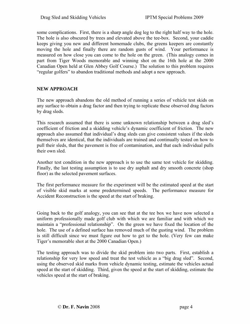
Returning to the golf analogy, we now require two shots to get on the green. The first shot gets us to the dog leg so we can see the green (vehicle as drag sled) and the second shot gets us on the green (vehicle dynamic skidding) and hopefully near the hole and then sinking the ball (speed at start of braking). We have abandoned the hole in one strategy for a birdie at best but an easy par. THE RESEARCH IN GENERAL The aim of the research is to provide a continuous analytical path through from the individual drag sled’s coefficient of friction to the estimated speed at the start of braking. The research has three parts; the first part is to treat the sled as a solid tire. The second part utilizes a known but unexplored relationship of the average coefficient of friction of a skidding vehicle and the speed at start of skid. The third part estimates the speed at the start of braking. The reader will observe, as they go through this paper that there is no mention of “drag factor”. The reason for this is important and will be explained later in the discussion. Part 1. Solid Tire Vehicle The first task of the research is to establish an acceptable relationship between an individual’s drag sled and a vehicle treated as a drag sled as hypnotized in Figure 1.

TYPICAL DRAG SLED AND VEHICLE RESULTS

0

0.1

0.2

0.3

0.4

0.5

0.6

0.7

0.8

0.9

1

0 20 40 60 80 100

Some Measure of Performance

Dra

g Fa

ctor

s/ C

oeffi

cien

t of F

rictio

n

120

FIGURE 1. HYPOTHETICAL RELATIONSHIP BETWEEN DRAG SLEDS AND VEHICLE-AS-DRAG-SLED

The trick here is to develop the relationship for a solid tire vehicle that has solid tires that are in fact manufactured drag sleds. In this experiment the solid tire drag sled’s tires are

?Individual’s Drag Sled

Vehicle as a Drag Sled



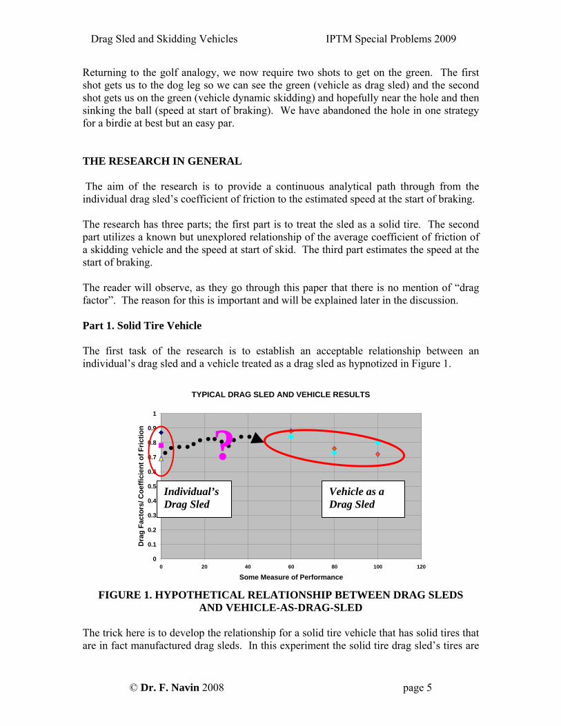
the same as those used for the individual drag sleds. The speed of the pulling is about the same used by individuals pulling a drag sled. The relationship developed will probably be unique to the drag sleds used in the experiment. Part 2. Vehicle-as-Drag-Sled and a Skidding Vehicle There is considerable data reported on the “drag factor” or average coefficient of friction of skidding vehicles on dry pavements at speeds above 25mph. One of the significant contributions of this research is to combine the Vehicle-as-Drag-Sled with the information from a skidding vehicle. Figure 2 is a hypothetical relationship between the dynamic coefficient of friction and the speed at the start of skid. The research must join the information in Figure 1 and Figure 2 into a single equation to estimate a vehicle’s dynamic coefficient of friction based on the speed at the start of skid marks.

DRAG FACTORS AND VEHICLE SPEEDHypothetical Data

0

0.1

0.2

0.3

0.4

1

0 20 40 60 80 100 120

Vehicle Speed, mph

Coe

ffici

en

FIGURE 2. DRAG FACTOR AND VEHICLE SPEED

Part 3. Estimate Vehicle’s Speed at the Start of Braking The first two parts of the research deals with the vehicle during the time it leaves visible skid marks. This last part adds the additional speed that is lost during the initial braking when no skid marks are left.

0.5

0.6

0.7

0.8

0.9

t of F

rictio

n, g

Vehicle as a Drag Sled



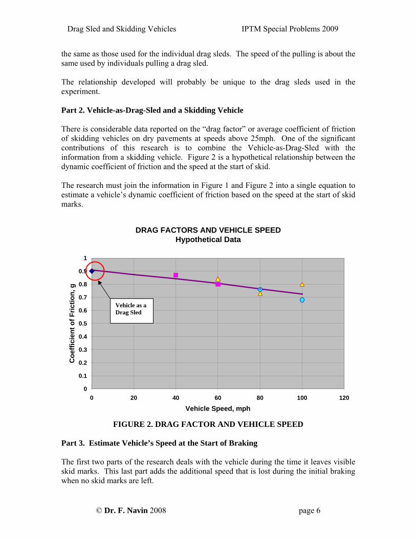
THE RESEARCH APPLICATION The research is divided into three parts. Thdata by a load cell at very slow speed. The and the third estimates the speed at the start of braking. Part 1. Individual Drag Sled and “Vehicle-as-Drag-Sled” To find the relationship between the coefdrag sled and a vehicle as a drag sled The solution was to build a big drag sled various weights. The big drag sled “tires” weindividuals. The big drag of carrying a car. Another device was one si“individual drag-sleds” as tireswere pulled with a tow truck’s winch at a the individual drag sled which were pulled individual drag sled force was measured either by

SOLID TI

e first deals with the drag sled and collecting second part incorporates the skidding vehicle

ficient of friction values of the individual’s proved to be surprisingly simple.

that could represent a solid tire vehicle of re drag sleds identical to those used by the

sled had four “individual drag-sleds” as tires and was capable ngle rail of the big drag sled with two

and of course individual drag-sleds. All the drag sleds speed of about 0.3mph (0.09m/s), except for

by hand at a slightly slower speed. The a load cell or a simple spring scale.

FIGURE 3 RE VEHICLE DEVICES

4 sled

4 sled

2 sled car sled


The typical set up for the experiment is shown in Figure 3. The appropriate load cell was used so the precision of the measurement was about 0.01%. A new area of the pavement surface was always used for testing. The data was recorded from the time that the pull was started. Usually the pull was released and then applied again for three applications. Some pulls were more stable then others. For example, the four sled vehicle was stable during pulling and a single heavily loaded drag sled tended to wiggle. The results reported are those considered stable over the three pulls. The data collected included the total weight of the device, the weight of the pulling assembly, the area of the tire footprint and the actual loaded area, and the force to pull the device. Each pull used a load cell and was repeated three times except for some of the individual drag sled pulls. Part 2. “Vehicle as Drag Sled”, Skidding Vehicle and Speed at Start of Skid Marks The dynamic vehicle skids were carried out in the usual manner. The experiment used the same vehicle (a police cruiser), same driver plus passenger and each speed was repeated three times. The surfaces were cleaned either by sweeping as was the case for the smooth concrete or for the asphaltic concrete, the previous day’s intense rain. The speed was recorded by radar and a VC3000. There was a shot marker. The visible skid marks were also recorded in the manner used by the RCMP. The vehicle was weighed as were the occupants. The speed at the start of braking was estimated as will be explained below. Part 3. Estimating Speed at Start of Braking Reed and Keskin (1987), Neptune (1995), Goudie et al (2000) and others have shown that there is a mathematical relationship between the speed at the start of visible skid marks and the speed at the start of braking. The data collected during this research included the speed at the start of braking measured by a VC3000 and radar EXPERIMENTAL RESULTS The results are for the Prince George experiment only. Additional information from the literature and other experiments by the author and his colleagues will be incorporated later. Part 1. Individual Drag Sled and “Vehicle-as-Drag-Sled” Relationship The experimental results on a dry asphalt pavement (parking lot) and a smooth concrete shop floor are shown in Figure 4. The plot illustrates a relationship between the



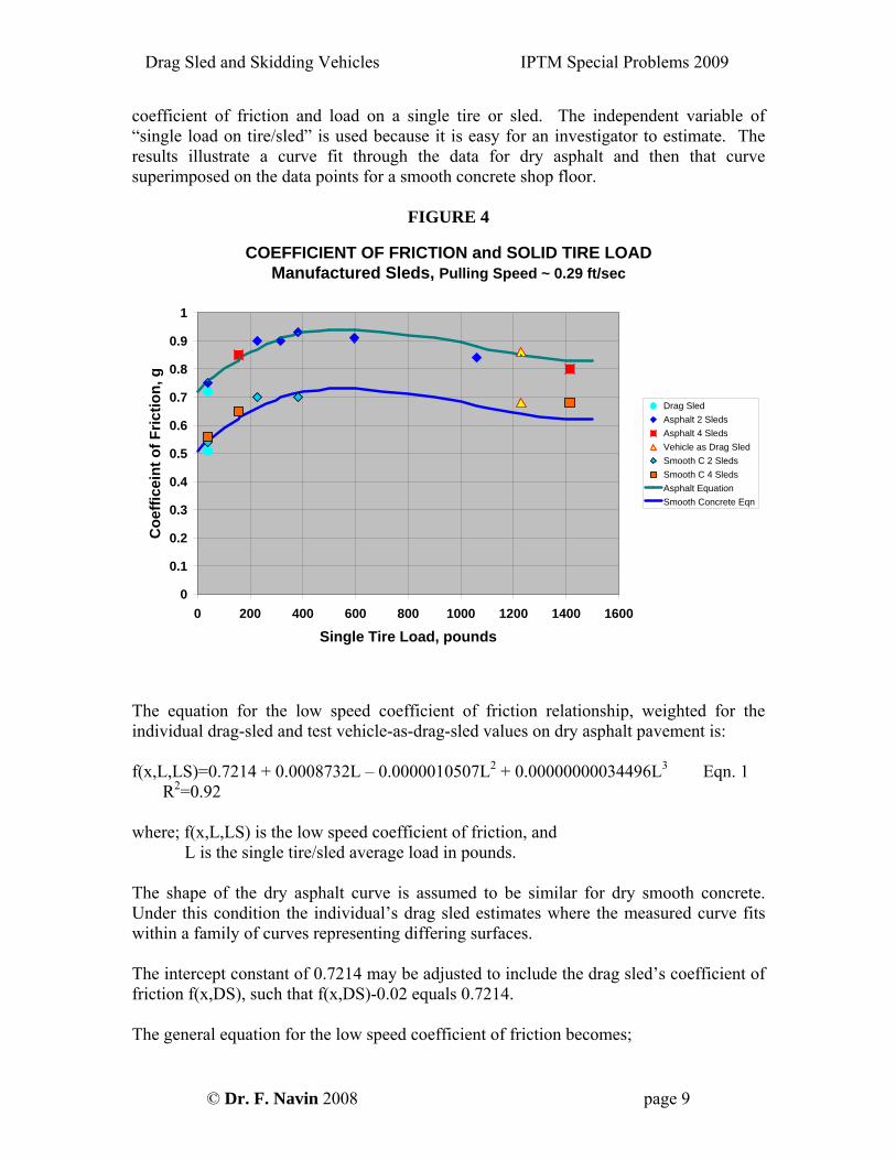
coefficient of friction and load on a single tire or sled. The independent variable of “single load on tire/sled” is used because it is easy for an investigator to estimate. The results illustrate a curve fit through the data for dry asphalt and then that curve superimposed on the data points for a smooth concrete shop floor.

FIGURE 4

COEFFICIENT OF FRICTION and SOLID TIRE LOADManufactured Sleds, Pulling Speed ~ 0.29 ft/sec

0

0.1

0.2

0.3

0.4

0.5

0.6

0.7

0.8

0.9

1

0 200 400 600 800 1000 1200 1400 1600

Single Tire Load, pounds

Coe

ffice

int o

f Fric

tion,

g

Drag SledAsphalt 2 SledsAsphalt 4 SledsVehicle as Drag SledSmooth C 2 SledsSmooth C 4 SledsAsphalt EquationSmooth Concrete Eqn

The equation for the low speed coefficient of friction relationship, weighted for the individual drag-sled and test vehicle-as-drag-sled values on dry asphalt pavement is: f(x,L,LS)=0.7214 + 0.0008732L – 0.0000010507L2 + 0.00000000034496L3 Eqn. 1 R2=0.92 where; f(x,L,LS) is the low speed coefficient of friction, and

L is the single tire/sled average load in pounds. The shape of the dry asphalt curve is assumed to be similar for dry smooth concrete. Under this condition the individual’s drag sled estimates where the measured curve fits within a family of curves representing differing surfaces. The intercept constant of 0.7214 may be adjusted to include the drag sled’s coefficient of friction f(x,DS), such that f(x,DS)-0.02 equals 0.7214. The general equation for the low speed coefficient of friction becomes;



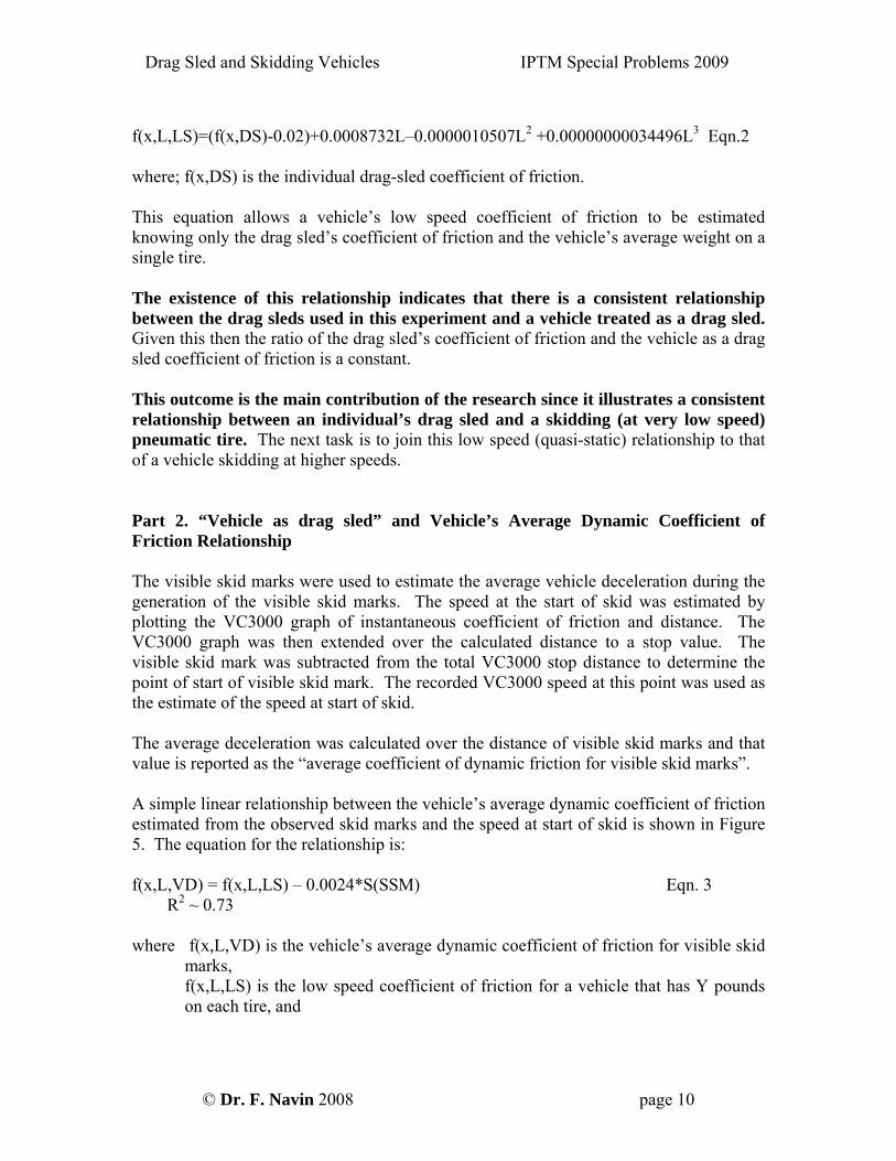
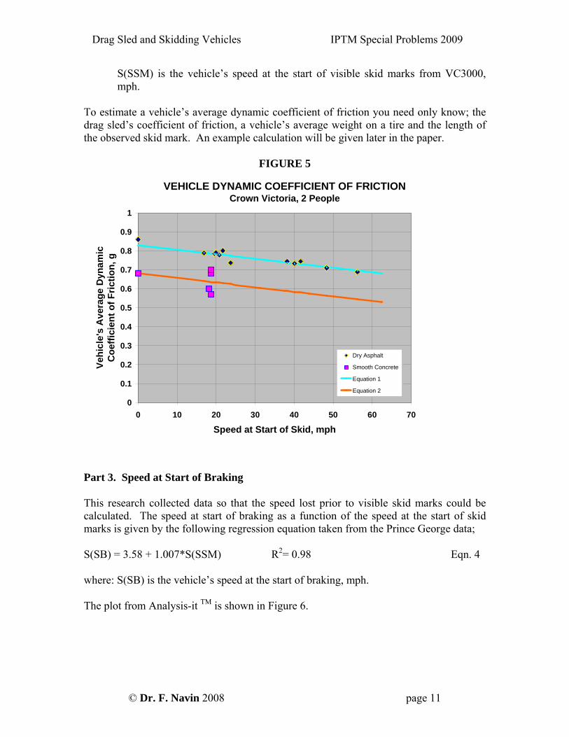
f(x,L,LS)=(f(x,DS)-0.02)+0.0008732L–0.0000010507L2 +0.00000000034496L3 Eqn.2 where; f(x,DS) is the individual drag-sled coefficient of friction. This equation allows a vehicle’s low speed coefficient of friction to be estimated knowing only the drag sled’s coefficient of friction and the vehicle’s average weight on a single tire. The existence of this relationship indicates that there is a consistent relationship between the drag sleds used in this experiment and a vehicle treated as a drag sled. Given this then the ratio of the drag sled’s coefficient of friction and the vehicle as a drag sled coefficient of friction is a constant. This outcome is the main contribution of the research since it illustrates a consistent relationship between an individual’s drag sled and a skidding (at very low speed) pneumatic tire. The next task is to join this low speed (quasi-static) relationship to that of a vehicle skidding at higher speeds. Part 2. “Vehicle as drag sled” and Vehicle’s Average Dynamic Coefficient of Friction Relationship The visible skid marks were used to estimate the average vehicle deceleration during the generation of the visible skid marks. The speed at the start of skid was estimated by plotting the VC3000 graph of instantaneous coefficient of friction and distance. The VC3000 graph was then extended over the calculated distance to a stop value. The visible skid mark was subtracted from the total VC3000 stop distance to determine the point of start of visible skid mark. The recorded VC3000 speed at this point was used as the estimate of the speed at start of skid. The average deceleration was calculated over the distance of visible skid marks and that value is reported as the “average coefficient of dynamic friction for visible skid marks”. A simple linear relationship between the vehicle’s average dynamic coefficient of friction estimated from the observed skid marks and the speed at start of skid is shown in Figure 5. The equation for the relationship is: f(x,L,VD) = f(x,L,LS) – 0.0024*S(SSM) Eqn. 3 R2 ~ 0.73 where f(x,L,VD) is the vehicle’s average dynamic coefficient of friction for visible skid

marks, f(x,L,LS) is the low speed coefficient of friction for a vehicle that has Y pounds on each tire, and



S(SSM) is the vehicle’s speed at the start of visible skid marks from VC3000, mph.

To estimate a vehicle’s average dynamic coefficient of friction you need only know; the drag sled’s coefficient of friction, a vehicle’s average weight on a tire and the length of the observed skid mark. An example calculation will be given later in the paper.

FIGURE 5

VEHICLE DYNAMIC COEFFICIENT OF FRICTIONCrown Victoria, 2 People

0

0.1

0.2

0.3

0.4

0.5

0.6

0.7

0.8

0.9

1

0 10 20 30 40 50 60 70

Speed at Start of Skid, mph

Vehi

cle'

s A

vera

ge D

ynam

ic

Coe

ffici

ent o

f Fric

tion,

g

Dry Asphalt

Smooth Concrete

Equation 1

Equation 2

Part 3. Speed at Start of Braking This research collected data so that the speed lost prior to visible skid marks could be calculated. The speed at start of braking as a function of the speed at the start of skid marks is given by the following regression equation taken from the Prince George data; S(SB) = 3.58 + 1.007*S(SSM) R2= 0.98 Eqn. 4 where: S(SB) is the vehicle’s speed at the start of braking, mph. The plot from Analysis-it TM is shown in Figure 6.



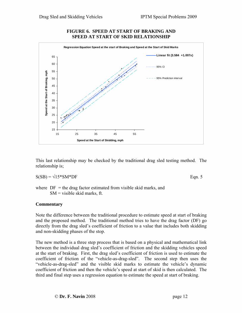
FIGURE 6. SPEED AT START OF BRAKING AND SPEED AT START OF SKID RELATIONSHIP

This last relationship may be checked by the traditional drag sled testing method. The relationship is; S(SB) = √15*SM*DF Eqn. 5 where DF = the drag factor estimated from visible skid marks, and SM = visible skid marks, ft. Commentary Note the difference between the traditional procedure to estimate speed at start of braking and the proposed method. The traditional method tries to have the drag factor (DF) go directly from the drag sled’s coefficient of friction to a value that includes both skidding and non-skidding phases of the stop. The new method is a three step process that is based on a physical and mathematical link between the individual drag sled’s coefficient of friction and the skidding vehicles speed at the start of braking. First, the drag sled’s coefficient of friction is used to estimate the coefficient of friction of the “vehicle-as-drag-sled”. The second step then uses the “vehicle-as-drag-sled” and the visible skid marks to estimate the vehicle’s dynamic coefficient of friction and then the vehicle’s speed at start of skid is then calculated. The third and final step uses a regression equation to estimate the speed at start of braking.

Regression Equation Speed at the start of Braking and Speed at the Start of Skid Marks

15

20

25

30

35

40

45

50

55

60

65

15 25 35 45 55

Speed at the Start of Skidding, mph

Spee

d at

the

Star

t of B

raki

ng, m

ph

Linear fit (3.584 +1.007x)

95% CI

95% Prediction interval




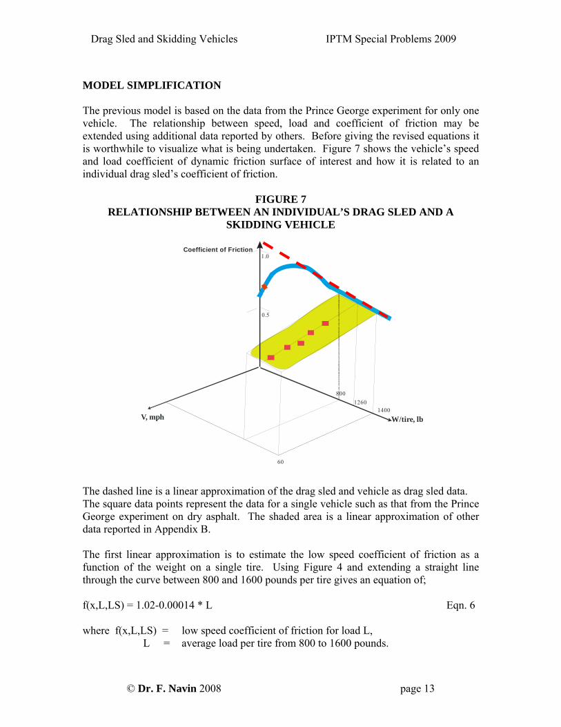
MODEL SIMPLIFICATION The previous model is based on the data from the Prince George experiment for only one vehicle. The relationship between speed, load and coefficient of friction may be extended using additional data reported by others. Before giving the revised equations it is worthwhile to visualize what is being undertaken. Figure 7 shows the vehicle’s speed and load coefficient of dynamic friction surface of interest and how it is related to an individual drag sled’s coefficient of friction.

FIGURE 7 RELATIONSHIP BETWEEN AN INDIVIDUAL’S DRAG SLED AND A

SKIDDING VEHICLE

12060

1260

400

Vehicle’s Dynamic Skid

V, km/h1400

800

1.0

0.5

V, mph W/tire, lb

Coefficient of Friction

The dashed line is a linear approximation of the drag sled and vehicle as drag sled data. The square data points represent the data for a single vehicle such as that from the Prince George experiment on dry asphalt. The shaded area is a linear approximation of other data reported in Appendix B. The first linear approximation is to estimate the low speed coefficient of friction as a function of the weight on a single tire. Using Figure 4 and extending a straight line through the curve between 800 and 1600 pounds per tire gives an equation of; f(x,L,LS) = 1.02-0.00014 * L Eqn. 6 where f(x,L,LS) = low speed coefficient of friction for load L,

L = average load per tire from 800 to 1600 pounds.


The equation may be revised to include the drag sled’s coefficient of friction as; f(x,L,LS) = f(x,DS) + 0.29 – 0.00014 * L Eqn. 7 where f(x,DS) = drag sled’s coefficient of friction. The linear approximation for the surface is then; f(x,L,VD) = f(x,DS) +0.29 – 0.0014 * L -0.0024 * S(SSM), Eqn. 8

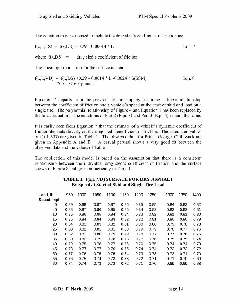
700>L<1601pounds Equation 7 departs from the previous relationship by assuming a linear relationship between the coefficient of friction and a vehicle’s speed at the start of skid and load on a single tire. The polynomial relationship of Figure 4 and Equation 1 has been replaced by the linear equation. The equations of Part 2 (Eqn. 3) and Part 3 (Eqn. 4) remain the same. It is easily seen from Equation 7 that the estimate of a vehicle’s dynamic coefficient of friction depends directly on the drag sled’s coefficient of friction. The calculated values of f(x,L,VD) are given in Table 1. The observed data for Prince George, Chilliwack are given in Appendix A and B. A casual perusal shows a very good fit between the observed data and the values of Table 1. The application of this model is based on the assumption that there is a consistent relationship between the individual drag sled’s coefficient of friction and the surface shown in Figure 8 and given numerically in Table 1.

TABLE 1. f(x,L,VD) SURFACE FOR DRY ASPHALT By Speed at Start of Skid and Single Tire Load

Load, lb 950 1000 1050 1100 1150 1200 1250 1300 1350 1400Speed, mph

0 0.89 0.88 0.87 0.87 0.86 0.85 0.85 0.84 0.83 0.825 0.88 0.87 0.86 0.85 0.85 0.84 0.83 0.83 0.82 0.81

10 0.86 0.86 0.85 0.84 0.84 0.83 0.82 0.81 0.81 0.8015 0.85 0.84 0.84 0.83 0.82 0.82 0.81 0.80 0.80 0.7920 0.84 0.83 0.83 0.82 0.81 0.80 0.80 0.79 0.78 0.7825 0.83 0.82 0.81 0.81 0.80 0.79 0.79 0.78 0.77 0.7630 0.82 0.81 0.80 0.79 0.79 0.78 0.77 0.77 0.76 0.7535 0.80 0.80 0.79 0.78 0.78 0.77 0.76 0.75 0.75 0.7440 0.79 0.78 0.78 0.77 0.76 0.76 0.75 0.74 0.74 0.7345 0.78 0.77 0.77 0.76 0.75 0.74 0.74 0.73 0.72 0.7250 0.77 0.76 0.75 0.75 0.74 0.73 0.73 0.72 0.71 0.7055 0.76 0.75 0.74 0.73 0.73 0.72 0.71 0.71 0.70 0.6960 0.74 0.74 0.73 0.72 0.72 0.71 0.70 0.69 0.69 0.68



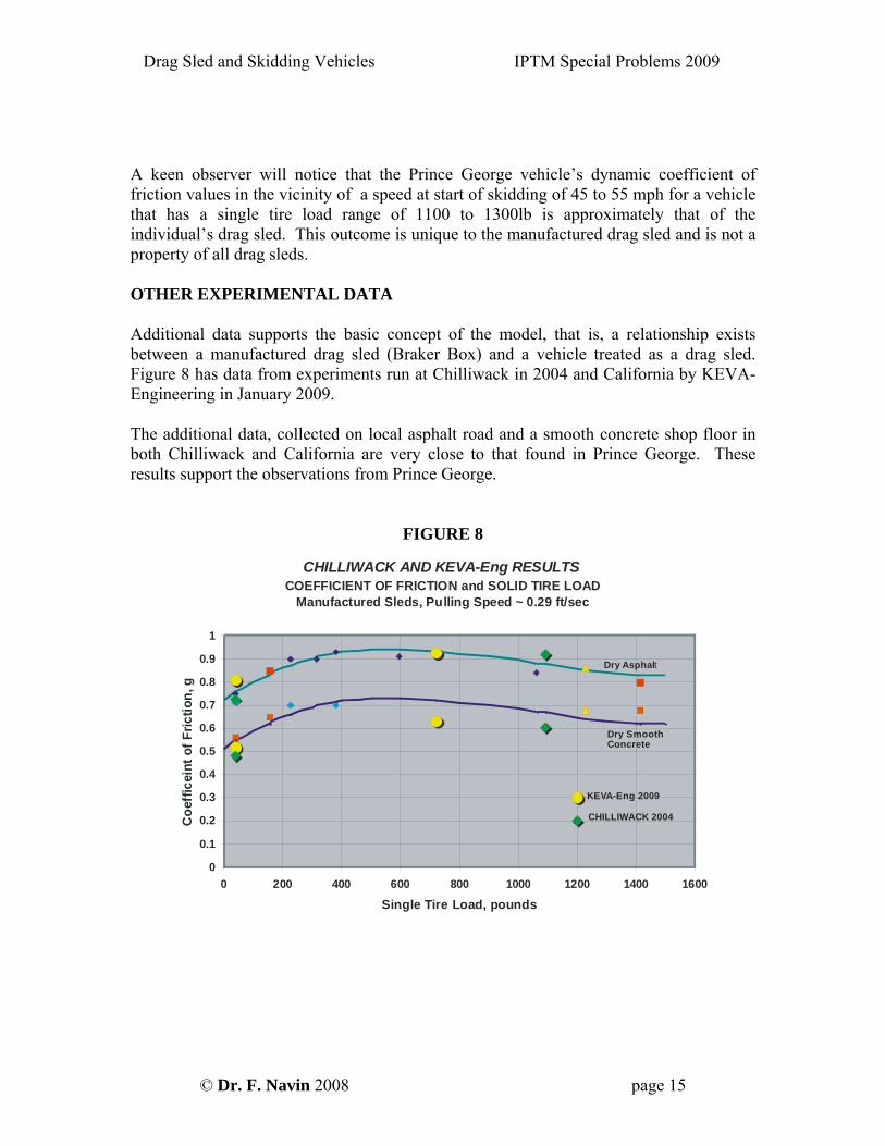
A keen observer will notice that the Prince George vehicle’s dynamic coefficient of friction values in the vicinity of a speed at start of skidding of 45 to 55 mph for a vehicle that has a single tire load range of 1100 to 1300lb is approximately that of the individual’s drag sled. This outcome is unique to the manufactured drag sled and is not a property of all drag sleds. OTHER EXPERIMENTAL DATA Additional data supports the basic concept of the model, that is, a relationship exists between a manufactured drag sled (Braker Box) and a vehicle treated as a drag sled. Figure 8 has data from experiments run at Chilliwack in 2004 and California by KEVA-Engineering in January 2009. The additional data, collected on local asphalt road and a smooth concrete shop floor in both Chilliwack and California are very close to that found in Prince George. These results support the observations from Prince George.

FIGURE 8

CHILLIWACK AND KEVA-Eng RESULTSCOEFFICIENT OF FRICTION and SOLID TIRE LOAD

Manufactured Sleds, Pulling Speed ~ 0.29 ft/sec

0

0.1

0.2

0.3

0.4

0.5

0.6

0.7

0.8

0.9

1

0 200 400 600 800 1000 1200 1400 1600

Single Tire Load, pounds

Coe

ffice

into

fFric

tion,

g

Dry Asphalt

Dry SmoothConcrete

KEVA-Eng 2009

CHILLIWACK 2004



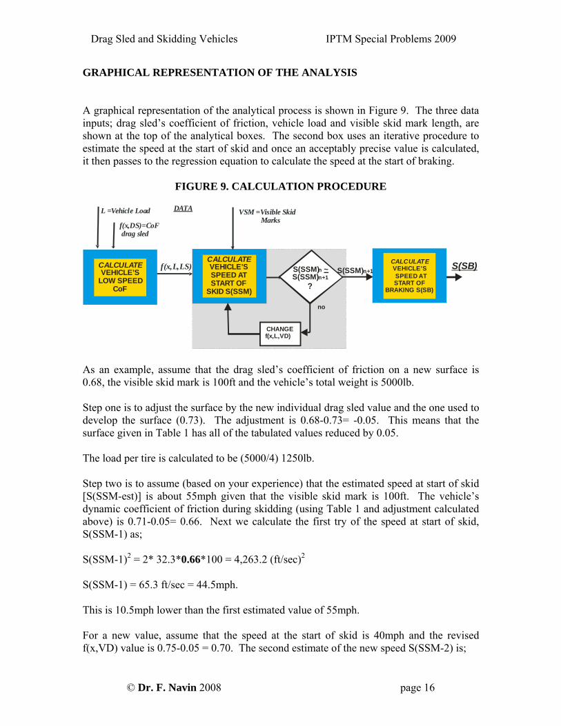
GRAPHICAL REPRESENTATION OF THE ANALYSIS A graphical representation of the analytical process is shown in Figure 9. The three data inputs; drag sled’s coefficient of friction, vehicle load and visible skid mark length, are shown at the top of the analytical boxes. The second box uses an iterative procedure to estimate the speed at the start of skid and once an acceptably precise value is calculated, it then passes to the regression equation to calculate the speed at the start of braking.

FIGURE 9. CALCULATION PROCEDURE

L =Vehicle Load DATA

f(x,L,LS)

f(x,DS)=CoF drag sled

CALCULATEVEHICLE’S

LOW SPEEDCoF

VSM =Visible Skid Marks

S(SSM) S(SSM)

nn+1

~

?

no

CHANGEf(x,L,VD)

CALCULATEVEHICLE’S SPEED ATSTART OF

BRAKING S(SB)

S(SB)S(SSM)n+1

CALCULATEVEHICLE’SSPEED ATSTART OF

SKID S(SSM)

As an example, assume that the drag sled’s coefficient of friction on a new surface is 0.68, the visible skid mark is 100ft and the vehicle’s total weight is 5000lb. Step one is to adjust the surface by the new individual drag sled value and the one used to develop the surface (0.73). The adjustment is 0.68-0.73= -0.05. This means that the surface given in Table 1 has all of the tabulated values reduced by 0.05. The load per tire is calculated to be (5000/4) 1250lb. Step two is to assume (based on your experience) that the estimated speed at start of skid [S(SSM-est)] is about 55mph given that the visible skid mark is 100ft. The vehicle’s dynamic coefficient of friction during skidding (using Table 1 and adjustment calculated above) is 0.71-0.05= 0.66. Next we calculate the first try of the speed at start of skid, S(SSM-1) as; S(SSM-1)2 = 2* 32.3*0.66*100 = 4,263.2 (ft/sec)2 S(SSM-1) = 65.3 ft/sec = 44.5mph. This is 10.5mph lower than the first estimated value of 55mph. For a new value, assume that the speed at the start of skid is 40mph and the revised f(x,VD) value is 0.75-0.05 = 0.70. The second estimate of the new speed S(SSM-2) is;



S(SSM-2)2 = 2* 32.3*0.70*100 = 4,522.0 (ft/sec)2 S(SSM-2) = 67.3 ft/sec = 45.9mph. This value is greater than the estimated value of 40mph. The two results bracket the answer so the most likely speed at the start of skid is about 45mph, this has a new f(x,VD) value of 0.74-0.05 = 0.69. The new speed estimate S(SSM-3) is; S(SSM-3)2 = 2* 32.3*0.69*100 = 4,457.4 (ft/sec)2 S(SSM-3) = 66.7 ft/sec = 45.5mph This is very close to the assumed 45mph. Therefore set S(SSM) equal to 45mph. The speed at the start of braking is then estimated by Equation 4; S(SB) = 3.58 + 1.007*S(SSM) S(SB) = 3.58 + 1.007* 45 = 48.9 = 49mph This example illustrates how the calculation procedure uses successive approximations. Remember that the underlying assumption is; a direct relationship exists between the individual drag sled’s coefficient of friction and the vehicle’s dynamic coefficient of friction for a particular single tire load and the speed at start of skid. And that there is a simple relationship between the speed at the start of braking and the speed at the start of visible skid marks.



CONCLUSIONS Establishing a relationship between an individual’s drag sled coefficient of friction and that of a skidding vehicle was a formidable challenge. The main hurdle was to abandon the traditional methods of analysis and find a new approach that utilized the capabilities of modern instrumentation. The new approach was to first emulate a “solid wheel vehicle” over a broad range of tire loads from the low of an individual’s drag sled to slightly beyond that of a mid size automobile. A load cell was used to measure the coefficient of friction at very low speed. The observations were compared to an automobile that was treated as a “vehicle as drag sled” and pulled at the same speed. The result was a polynomial equation relating; the drag sled coefficient of friction, the “solid tire vehicle” coefficient of friction and the vehicle as a drag sled to the average load on a single tire or sled. The relationship gives similar results for both asphalt and smooth concrete. The second step in the new approach was to establish a relationship between the “vehicle-as-drag-sled” coefficient of friction and the “vehicle’s average dynamic coefficient of friction” at the start of skid. A series of traditional skid tests were run at speeds of approximately 25, 45 and 55mph and the skid marks recorded. A simple linear relationship was established between the “vehicle’s average dynamic coefficient of friction” , the speed at the start of skid marks and average load on a tire. The final step is to estimate the speed at the start of braking given the speed at the start of skidding with a simple regression equation. There is a continuous mathematical and experimental link between the drag sled’s coefficient of friction, the “vehicle-as-drag-sled’s” coefficient of friction, the vehicle’s average coefficient of friction and the start of skid marks and the start of braking. The results also show that drag sleds work for the dry asphalt surface such as that tested at Prince George, British Columbia using drag sleds from a local manufacturer (Braker Box), RCMP officers as pullers and RCMP pulling protocols, that is, individuals trained and skilled in the use of drag sleds. The new method was simplified by replacing the original polynomial equation with a linear relationship between the coefficient of friction at very low speed and the load on a single tire. This simplified method works well within the vehicle load range of interest and greatly simplifies the calculations. This research should finally reduce the intensity of the ongoing “Drag Sled Wars” to that of minor skirmishes over testing details.



ACKNOWLEDGEMENTS These experiments and research program started in the spring of 2004. The author’s involvement in coefficient of friction research started in 1975. An experimental program of this complexity and difficulty requires the contributions of many individuals and organizations. IPTM (D Brill, P.E.) has generously provided much of the financial support for the purchase of material, rental of equipment and travel for some observers. The RCMP “E” Division Traffic Services (Inspector E Brewer, Sgt D. Williams and many others) has provided personal, vehicles and found suitable test sites in both Chilliwack and Prince George. Innovative Vehicle Testing Ltd. (R Baerg, P.Eng) did much of the load cell drag testing in 2004 and 2008. MEA Forensic Inc. (J Lawrence, P.Eng) helped with the skid testing and analysis in 2004. X Gao of UBC Civil Engineering Graduate Program did the data analysis in 2004. Dr. P. Musa of Hamilton Associates set up the Analysis of Variance experimental design for 2004. Additional financial support came from SYNECTICS Road Safety Research Corp. KEVA Engineering LLP (Micheal Varat, PE, John Kerkhoff and others) of Camarillo, California performed low speed load cell tests with a different vehicle on both dry asphalt and smooth concrete in January 2009. Officer John Grindey of California Highway Patrol provided expert drag sled help. The help from all these individuals and institutions is very much appreciated. Their help does not necessarily imply support for the drag sled procedure. Any errors or omissions are those of the author. REFERENCES Bartlett, W., Baxter, A., et al., Comparison of Drag-Sled and Skidding-Vehicle Drag Factors on Dry Roadways, SAE Paper 2006-01-1398, Warrendale PA., 2006. Goudie, D., Bowler, J., Brown,C., Hemrichs, B., Siegmund, G., Tire Friction During Locked Wheel Braking, SAE Paper 2000-01-1314, Warrendale, PA, 2000. Neptune, J., Flynn, J., Chavez, P, Underwood, H., Speed from Skids: A Modern Approach, SAE Paper 950354, Warrendale, PA, 1995. Reed, W., Keksin, A., Vehicle Response to Emergency Braking, SAE Paper 87051, Warrendale, PA, 1987




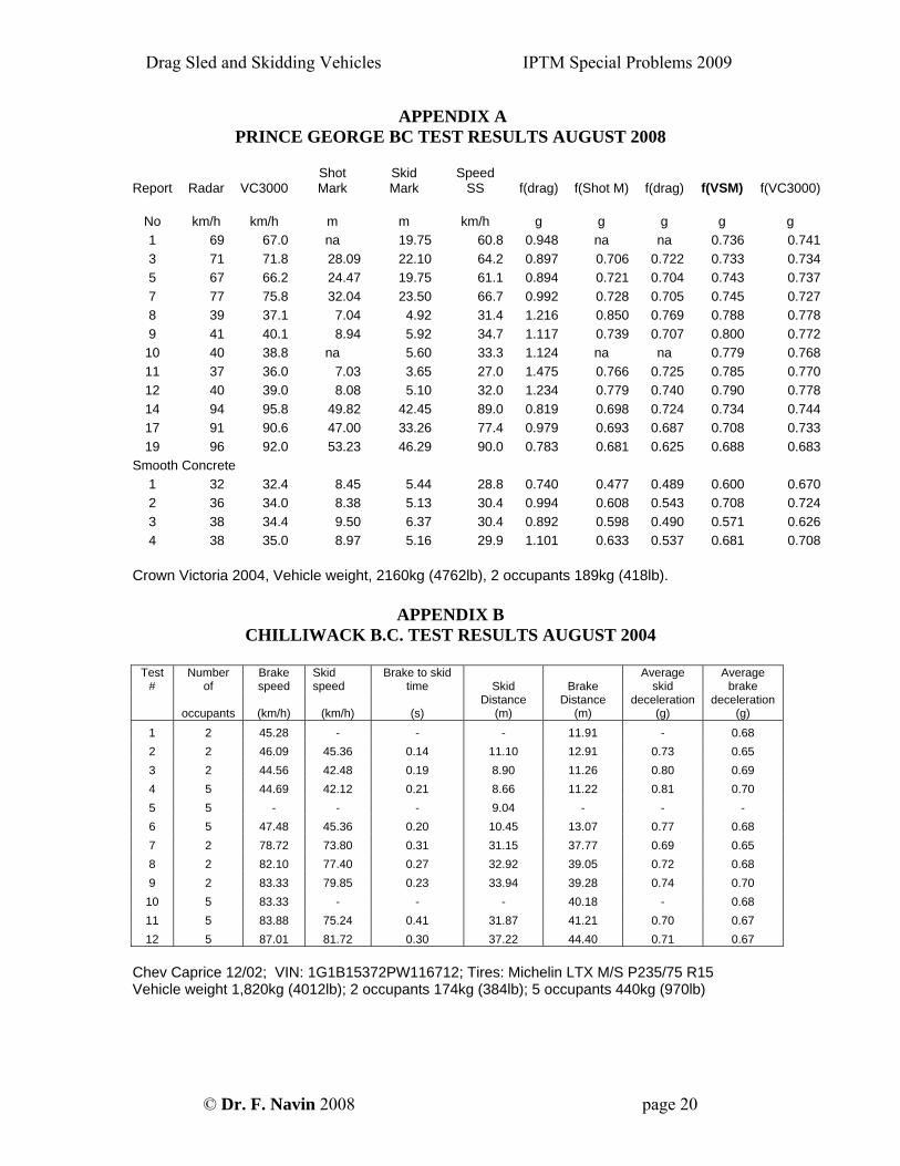
APPENDIX A PRINCE GEORGE BC TEST RESULTS AUGUST 2008

Report Radar VC3000 Shot Mark

Skid Mark

Speed SS f(drag) f(Shot M) f(drag) f(VSM) f(VC3000)

No km/h km/h m m km/h g g g g g 1 69 67.0 na 19.75 60.8 0.948 na na 0.736 0.741 3 71 71.8 28.09 22.10 64.2 0.897 0.706 0.722 0.733 0.734 5 67 66.2 24.47 19.75 61.1 0.894 0.721 0.704 0.743 0.737 7 77 75.8 32.04 23.50 66.7 0.992 0.728 0.705 0.745 0.727 8 39 37.1 7.04 4.92 31.4 1.216 0.850 0.769 0.788 0.778 9 41 40.1 8.94 5.92 34.7 1.117 0.739 0.707 0.800 0.772

10 40 38.8 na 5.60 33.3 1.124 na na 0.779 0.768 11 37 36.0 7.03 3.65 27.0 1.475 0.766 0.725 0.785 0.770 12 40 39.0 8.08 5.10 32.0 1.234 0.779 0.740 0.790 0.778 14 94 95.8 49.82 42.45 89.0 0.819 0.698 0.724 0.734 0.744 17 91 90.6 47.00 33.26 77.4 0.979 0.693 0.687 0.708 0.733 19 96 92.0 53.23 46.29 90.0 0.783 0.681 0.625 0.688 0.683

Smooth Concrete 1 32 32.4 8.45 5.44 28.8 0.740 0.477 0.489 0.600 0.670 2 36 34.0 8.38 5.13 30.4 0.994 0.608 0.543 0.708 0.724 3 38 34.4 9.50 6.37 30.4 0.892 0.598 0.490 0.571 0.626 4 38 35.0 8.97 5.16 29.9 1.101 0.633 0.537 0.681 0.708

Crown Victoria 2004, Vehicle weight, 2160kg (4762lb), 2 occupants 189kg (418lb).

APPENDIX B

CHILLIWACK B.C. TEST RESULTS AUGUST 2004

Test #

Number of

Brake speed

Skid speed

Brake to skid time Skid Brake

Average skid

Average brake

occupants (km/h) (km/h) (s) Distance

(m) Distance

(m) deceleration

(g) deceleration

(g)

1 2 45.28 - - - 11.91 - 0.68 2 2 46.09 45.36 0.14 11.10 12.91 0.73 0.65 3 2 44.56 42.48 0.19 8.90 11.26 0.80 0.69 4 5 44.69 42.12 0.21 8.66 11.22 0.81 0.70 5 5 - - - 9.04 - - - 6 5 47.48 45.36 0.20 10.45 13.07 0.77 0.68 7 2 78.72 73.80 0.31 31.15 37.77 0.69 0.65 8 2 82.10 77.40 0.27 32.92 39.05 0.72 0.68 9 2 83.33 79.85 0.23 33.94 39.28 0.74 0.70

10 5 83.33 - - - 40.18 - 0.68 11 5 83.88 75.24 0.41 31.87 41.21 0.70 0.67 12 5 87.01 81.72 0.30 37.22 44.40 0.71 0.67

Chev Caprice 12/02; VIN: 1G1B15372PW116712; Tires: Michelin LTX M/S P235/75 R15 Vehicle weight 1,820kg (4012lb); 2 occupants 174kg (384lb); 5 occupants 440kg (970lb)



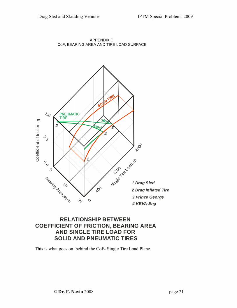
APPENDIX C, CoF, BEARING AREA AND TIRE LOAD SURFACE

Coe

ffici

e nt o

f fric

tion,

g

Bearing Area,sq-in

Single Tire

Load, lb

0

1200

2000

400

0.5

1.0

15

30

0.0

0

1

34

2

RELATIONSHIP BETWEENCOEFFICIENT OF FRICTION, BEARING AREA

AND SINGLE TIRE LOAD FOR SOLID AND PNEUMATIC TIRES

1 Drag Sled

2 Drag Inflated Tire

3 Prince George4 KEVA-Eng

This is what goes on behind the CoF- Single Tire Load Plane.

Documents

DRAG SLED AND AUTOMOBILE SKIDDING; AN ... George Research 2008...DRAG SLED AND AUTOMOBILE SKIDDING; AN ANALYTICAL RELATIONSHIP by Frank Navin, Ph.D., D.Sc.(Hon), P.Eng Professor Emeritus