Embed Size (px)
Citation preview

Week 2 Memo Drag and Lift Coefficients
Evan States, Zacarie Hertel, Eric Robinson
3/6/2013
“I affirm that I have carried out my academic
endeavors with full academic honesty.”
Signed Electronically,
Evan States, Zac Hertel, Eric Robinson

1
TO: Professor Anderson
FROM: Evan States, Zacarie Hertel, Eric Robinson – Students
DATE: March 8, 2013
SUBJECT: Lift and Drag on a Mercedes-Benz CLK Touring Car
Purpose:
This memo reports the results of our experiments to find the coefficients of drag and lift
on a 1:12 scale model Mercedes CLK Touring Car. Our model was mounted on a dynamometer
in the wind tunnel which measured both the drag and lift forces that the acted on the car at wind
speeds ranging from 0 to 42 m/s. The coefficient of drag from our experiments ranged from 2.0
(+/- .169) at a wind speed of 13.0(+/- .387) m/s to .75(+/- .050) at a wind speed of 42.4 (+/- .634)
m/s. The coefficient of lift from our experiments ranged from .414 to .281 with a wind speed of
6.25 m/s and 19.6 m/s respectively. We found that both of these numbers were dependent upon
Reynolds’ number until a certain point, roughly 3.0x10⁵, at which point the data becomes
independent of Reynolds’ number.
Setup:
Drag is the force that acts opposite to the path of the vehicle’s motion, while lift is the
force that acts on a vehicle normal to the road surface that the it on. We analyzed the lift and
drag coefficients of a scaled Mercedes CLK (information on the scaled model is listed in
Appendix 9) at 12 specific wind tunnel motor frequencies on the surface of the vehicle. The
model was pre-mounted to a dynamometer in the wind tunnel and a pressure transducer was
connected to the Pitot probe for wind velocity calculations. Data was taken with a computer data
acquisition system with 3 input channels. The first related to pressure, the second related to lift
force and the third related to drag force.
Summary:
Data from each of the three input channels were measured with a Static Pitot Probe at 12
different motor frequencies, ranging from 10 Hz to 54 Hz; these frequencies represent wind
speeds from 6.25 (+/- .677) m/s to 42.4 (+/- .634) m/s. The data tables for the velocity
calculations are in Appendix 5. These results closely match our results from previous
experiments in the wind tunnel.
The coefficient of lift on the Mercedes CLK ranged from .414 (+/- .196) at a simulated
velocity of 6.25 (+/- .197) m/s to .281(+/- .026) at 19.6 (+/- .391) m/s. The coefficients of drag
range from 2.0 (+/- .169) at a wind speed of 13.0(+/- .387) m/s to .75(+/- .050) at a wind speed of
42.4 (+/- .634) m/s. This data is shown in detail in Appendices 1 and 3, and is explained

2
extensively in Appendices 2 and 4. Detailed results are shown visually in Figure 1. Note that as
the Reynolds’ Number increases, the coefficients approach a constant state. This represents how
at a certain velocity, the coefficients are no longer a function of Reynolds’ Number.
When we reflect upon these numbers, we find that both the lift and drag coefficients are
not what we expected. One would think a high performance sports car would generate high down
force, whereas our car is experiencing lift. Also, a drag coefficient of 2.0 is quite high, and even
the lowest drag coefficient value of .75 is still too high for a high performance sports car. Upon
completion, we expected to see drag coefficient values of between 0.3 and 0.5. One possible
explanation of the distortion of our coefficients was the orientation of how our vehicle was
mounted in the wind tunnel. The nose of the Mercedes was pointing slightly up in the air
meaning the car was on an angle. This could have increased the frontal area, or forced some air
underneath the car, which would have further distorted the results.
Conclusion:
The values that were obtained from the experiment seem unreasonable, comparing more
to those of a blunt object than an aerodynamically tuned sports car. While the calculated
uncertainties in these values may be low, there are other issues that are not taken into account in
the uncertainty analysis, for example the angle at which the car was mounted would significantly
swing the data. The current results cannot be deemed valid, especially without another set of
values to compare them to. We recommend completing the experiment again, paying close
attention to how the vehicle is mounted in the wind tunnel. If you have any further questions or
concerns, please contact our group at [email protected].
Figure 1 – Demonstrates how the coefficients of lift and drag varied with an increasing
Reynolds’ Number. The Reynolds’ Number increases linearly with the changing wind speed.
The first 2 Drag Coefficient data points have been omitted due to the extreme uncertainty
associated with them. This uncertainty can be seen in Appendices 1 and 3.
0
0.5
1
1.5
2
2.5
0 2 4 6 8
Co
eff
icie
nt
Re x 100000
Lift Coef.
Drag Coef.

3
Appendices:
1. Coefficient of Lift Data Tables
2. Coefficient of Lift and CL Uncertainty Calculations
3. Coefficient of Drag Data Tables
4. Coefficient of Drag and CD Uncertainty Calculations
5. Velocity Data Tables and Calculations
6. Equations Used
7. Setup, Experimental Procedure, and Tasks
8. Car Data
9. References

Appendix 1: Coefficient of Lift Data Tables
Table 1 below shows the data found in the lab experiment. The equations and methods used are explained in depth on the next
page. One thing to note while looking at Table 1and Figure 2, is as the velocity of the wind increased, the lift force on the car also
increased, however their relationship is non-linear. The data from Table 2 is used in Figure 3 which shows the relationship between
the coefficient of lift and Reynolds’ Number. Notice that at a Reynolds’ Number of about 3x10⁵ the lift coefficient approaches a
constant of about .3. This signifies the point at which the Coefficient of Lift is no longer dependent upon Reynolds Number.
0
2
4
6
8
10
0 10 20 30 40 50
Lift
Fo
rce
(N
)
Wind Velocity (m/s)
Figure 2
Frequency (Hz) 10 14 18 22 26 30 34 38 42 46 50 54
Velocity (m/s) 6.255 9.625 12.972 16.328 19.651 22.988 26.272 29.570 32.868 36.129 39.295 42.445
Uncertainty in Velocity 0.677 0.466 0.387 0.362 0.391 0.397 0.437 0.471 0.516 0.562 0.608 0.654
Lift Force (N) 0.241 0.436 0.755 1.143 1.618 2.236 2.952 3.760 4.706 5.901 7.207 8.676
Uncertainty Lift F (N) 0.101 0.103 0.104 0.121 0.124 0.119 0.124 0.146 0.148 0.215 0.187 0.206
Frequency (Hz) 10 14 18 22 26 30 34 38 42 46 50 54
Coefficient of Lift 0.414 0.316 0.301 0.288 0.281 0.284 0.287 0.289 0.292 0.303 0.313 0.323
Uncertainty CL 0.196 0.081 0.046 0.034 0.026 0.020 0.018 0.017 0.016 0.017 0.016 0.016
Reynolds' Number 93992.5 144647.5 194936.1 245380.3 295312.3 345460.8 394805.2 444374.8 493927 542943.8 590517.4 637852.3
Viscosity (kg/ms) 1.98E-05
0
0.2
0.4
0.6
0.8
0 1 2 3 4 5 6 7Li
ft C
oef
fici
ent
Re
x 100000 Figure 3
Table 2
Table 1

Appendix 2: Coefficient of Lift Calculations with Uncertainties
Firstly, the average of the 100
voltage data points at each frequency
was found, and then the standard
deviation and the percent standard
deviation. Next, we took the averages
and used the calibration curve shown
in Figure 4 to the right to calculate the
lift force on the car at each of the
motor frequencies. Then, using
equation (1) in Appendix 6, we
calculated the coefficient of lift at each of
the motor frequencies. The coefficient of
lift at each of the subsequent motor frequencies can be viewed in Appendix 1, on the previous
page. The next step in our calculations was to calculate the uncertainties in both the lift force on
the car and the car’s coefficient of lift. The former calculation was completed using equation (9)
with the standard deviation of the lift force, and the uncertainty in the lift coefficient was found
using equation (10).
One trend that we have noticed in multiple experiments now, is that as the velocity of the
wind in the tunnel decreases, so too does the accuracy of our data. In other words, the uncertainty
rises as the velocity decreases, this is why in Figure 3 the uncertainties decreases as the
Reynolds’ Number increases.
As mentioned in the memo, the values of our lift data seem high. One would think that a
high performance race car such as this would produce immense down force in order to
strengthen cornering ability; however we observed a tendency for the car to lift off of the surface
on which it is driving. This is most likely caused by the angle at which the car was mounted in
the tunnel. This angle would affect our lift data by forcing more air under the car than over it,
thereby pushing the car up off of the road surface.
Figure 4 – this graph shows the Dynamometer Lift Force
Calibration we used to calculate our lift forces.

Appendix 3: Coefficient of Drag Data Tables
Table 3 below shows the resultant data from the drag experiment in the lab. The equations and methods used to obtain this data
are explained in depth on the next page. Figure 4 shows the relationship between the drag force on the car and the velocity of the wind
in the wind tunnel. Notice that as seen in Figure 2, this relationship is non-linear. Figure 5 shows the relationship between the drag
coefficient and the Reynolds’ Number of the flow of air. Note that here, Reynolds’ Number independence is achieved around 4.0x10⁵.
Frequency (Hz) 10 14 18 22 26 30 34 38 42 46 50 54
Coefficient of Drag 7.188 3.288 1.986 1.528 1.239 1.089 1.065 0.963 0.893 0.846 0.791 0.750
Uncertainty Cd 1.686 0.423 0.197 0.123 0.089 0.069 0.060 0.052 0.046 0.043 0.039 0.037
Reynold's Number 93992.5 144647.5 194936.1 245380.3 295312.3 345460.8 394805.2 444374.8 493927 542943.8 590517.4 637852.3
Viscosity (kg/ms) 1.98E-05
0
2
4
6
8
10
0 1 2 3 4 5 6 7
Co
eff
icie
nt
of
Dra
g
Re
x 100000 Figure 6
0
1
2
3
4
5
6
0 10 20 30 40 50
Dra
g Fo
rce
(N
)
Wind Velocity (m/s)
Figure 5
Table 3
Table 4
Frequency (Hz) 10 14 18 22 26 30 34 38 42 46 50 54
Velocity (m/s) 6.255 9.625 12.972 16.328 19.651 22.988 26.272 29.570 32.868 36.129 39.295 42.445
Uncertainty in Velocity 0.677 0.466 0.387 0.362 0.391 0.397 0.437 0.471 0.516 0.562 0.608 0.654
Drag Force (N) 1.174 1.271 1.395 1.700 1.997 2.402 3.067 3.515 4.025 4.606 5.097 5.637
Uncertainty Drag F 0.100 0.101 0.102 0.102 0.104 0.104 0.105 0.109 0.112 0.122 0.127 0.131

Appendix 4: Coefficient of Drag Calculations with Uncertainties
Again, the first step was to find the
average of the 100 voltage data points at
each frequency, and then the standard
deviation and finally, the percent standard
deviation. After, we used the calibration
curve shown to the right in Figure 7 to
calculate the drag forces at each of the 12
motor frequencies. From here on out, the
calculations are very similar to those used
for the lift force and coefficient
calculations. Equation (1) was used to
find the coefficient of drag, equation (9)
was used to find the uncertainty in the drag force, and equation (10) was used to calculate the
uncertainty in the coefficient of drag.
The drag forces calculated in this lab seem to be quite large, but as mentioned previously,
the car was mounted on an angle in the tunnel and that could have had a substantial effect on the
resulting data. This would have increased the frontal area, which would have greatly increased
the drag force on the car, and it also would have directed more air under the car, which would
help to explain the high lift forces shown and explained in Appendices 1 and 2.
Figure 7 – this graph shows the Dynamometer Drag Force
Calibration we used to calculate our lift forces.

Appendix 5: Velocity Data Tables and Calculations
Tables 5 and 6 show the velocity data obtained in the wind tunnel. We
calculated the pressures at each motor frequency and then used those pressures to
calculate the velocity of the wind at each motor frequency. These calculated
velocities were then in turn used for the calculations of the Reynolds’ Numbers. The
equation used to calculate the Reynolds’ Number is equation (8) in Appendix 6.
These numbers compare very directly to the velocity and pressure calculations from
last week’s report.
In order to calculate the wind velocity at each frequency, we had to first use
the calibration curve shown in figure 8 to find the average pitot probe pressures at
each frequency. Then, we used the pitot probe pressures along with the density of
the air in equation (4) in Appendix 6 to find the wind velocity of each motor
frequency. The final step of the velocity analysis was to calculate the uncertainty in
pitot probe pressure using equation (5). Lastly, we used the results from the
uncertainty in pressures to find the uncertainties in velocity using equation (7).
Frequency (Hz) Test 10 14 18 22 26 30 34 38 42 46 50 54
Pressure (Pa) -1.937 23.316 55.218 100.287 158.905 230.156 314.961 411.363 521.144 643.850 777.981 920.290 1073.741
Velocity (m/s) 1.803 6.255 9.625 12.972 16.328 19.651 22.988 26.272 29.570 32.868 36.129 39.295 42.445
% unc. V 1.287 0.108 0.048 0.030 0.022 0.020 0.017 0.017 0.016 0.016 0.016 0.015 0.015
Uncertainty in V (m/s) 2.321 0.677 0.466 0.387 0.362 0.391 0.397 0.437 0.471 0.516 0.562 0.608 0.654
Reynolds' Number 27093.113 93992.504 144647.471 194936.093 245380.260 295312.341 345460.763 394805.197 444374.786 493927.028 542943.807 590517.373 637852.270
Viscosity (kg/ms) 1.98E-05
Frequency (Hz) Test 10 14 18 22 26 30 34 38 42 46 50 54
Δ Pressure (inH2O) -0.008 0.094 0.222 0.403 0.639 0.925 1.266 1.653 2.095 2.588 3.127 3.699 4.316
Uncertainty Pressure (inH20) 0.020 0.020 0.020 0.021 0.021 0.024 0.021 0.023 0.021 0.022 0.023 0.025 0.026
Density (kg/m^3) 1.192 0.036Uncert. in Density
Table 5
Table 6
Figure 8

Appendix 6: Equations Used
Firstly, the two most important equations used in this lab are as follows:
(1) and
(2)
Where CL is the coefficient of lift, FL is the actual lift force the car is experiencing, CD is the drag
coefficient, FD is the drag force, ρ is the density of the air, V is the velocity of the air and AF is
the frontal area of the car. Equations 1 and 2 were used to calculate the lift and drag coefficients
of the car.
The Ideal Gas Law, which was used to calculate the density and uncertainty in density is:
(3)
Where P is the Pressure in the chamber, is the density, R is the ideal gas constant, and T is the
temperature of the air in Kelvin.
Another very important equation, integral to the calculation of the velocity of the wind is
√
(4)
Where V is the velocity of the air, is the pitot probe pressure and is the density of the air.
The Uncertainty in the pitot probe pressure was calculated using equation 5:
√ (5)
The Uncertainty in density was calculated using the following equation which was
derived from the ideal gas law is:
√
(
) (6)
The uncertainty in the velocity of the air was calculated using the equation:
√(
)
(7)
The equation used to solve for the Reynolds’Number is:
(8)
The uncertainty in the lift force is found using Equation 9 below:
√ (9)
The uncertainty in the coefficient of lift was found using:
√
(10)
The uncertainty in the drag force is found using:
√ (11)
The uncertainty in the coefficient of drag was found using:
√
(12)
1
Appendix 7: Setup, Experimental Procedure, and Tasks
Introduction:
The purpose of this week’s lab exercise is to measure the lift and drag forces acting on the radio
controlled vehicle that your group is studying. Drag is the force that acts opposite to the path of
the vehicle’s motion. It is detrimental to vehicle performance because it limits the top speed of a
vehicle and increases the fuel consumption, both of which are negative consequences for race
vehicles. Low drag vehicles usually have one or some combination of the following
characteristics: streamlined shape, low frontal area, and minimal openings in the bodywork for
windows or cooling ducts. The drag performance of vehicles is characterized by the drag
coefficient (CD) which is defined as:
(1)
Where FD is the drag force, ρ is the air density, V is the free stream velocity, and AF is the
frontal area of the vehicle. This non-dimensional coefficient allows the drag performance
between different vehicles and different setups of the same vehicle to be compared directly.
Lift is the other of the two main aerodynamic forces imposed on a race vehicle, but unlike drag,
lift can be manipulated to enhance the performance of a racecar and decrease lap times. Lift is
the force that acts on a vehicle normal to the road surface that the vehicle rides on. As its
definition implies, lift usually has the effect of “pulling” the vehicle upwards - away from the
surface it drives on. However, by manipulating the racecar geometry it is possible to create
negative lift, or down-force. Down-force enhances vehicle performance by increasing the normal
load on the tires. This increases the potential cornering force which results in the ability of the
vehicle to go around corners faster and reduce lap times. The lift of the vehicle is characterized
by the lift coefficient (CL) and is defined as:
(2)
Where FL is the lift force, AT is the area of the top surface of the vehicle (see Table 1), and the
other variables are as defined above. A negative lift coefficient means that a vehicle is
experiencing down force (Note: See last week’s lab handout for frontal and top area information
on your vehicle).
Procedure
The race car body will be pre-mounted in the wind tunnel for you and the pressure transducer has
been pre-calibrated (use the same calibration that you used for the surface pressure
measurements).
You will be provided with calibration data for the dynamometer.
Setup Steps:
1. Note any experimental observations about how the car is mounted in the wind tunnel.
Note the room temperature for your density calculation.
2. Make sure that the pressure transducer output is connected to channel 1, the
dynamometer lift (blue/black, blue wire) is connected to channel 2 and the dynamometer
drag.

2
3. Check the connections on the wind tunnel pitot probe. The stagnation pressure (vertical
tap) should be connected to the “total” connection on the back of the pressure transducer
and the static pressure (horizontal tap) should be connected to the “static” tap on the back
of the pressure transducer and the pressure selector switch should be set to channel 0.
4. Start Excel and make sure the Daq software is running. Check that the data acquisition is
set to read channels 1, 2 and 3 (-10to +10V) and record 100 readings at a rate of about 6
Hz.
5. With the wind tunnel off, start the data acquisition program and read the data on channels
1, 2 and 3. Since there is no flow all three should be close to zero. Confirm this before
proceeding. If the lift and drag values are not zero (or less than .05 V) you will need to
re-zero the lift and drag system using the two brass thumb wheels mounted directly on
the dynamometer to account for the weight of your car model. DO NOT adjust the span
or zero dials for the lift or drag on the wind tunnel instrumentation box. These are the
dials that are helpfully labeled “do not touch.”
6. Set the wind tunnel speed to 10 Hz and turn on the wind tunnel.
7. Acquire and save your data. Note: a negative Lift value implies down force and a positive
Drag value implies Drag (in direction of flow).
8. Increment the wind tunnel speed by 4 Hz, and repeat step 7 until the wind tunnel speed is
54 Hz. Be sure to allow the system stabilize for a minute or so after you change each
wind speed
9. Save your output file and move to another computer to perform your data reduction.
Data Reduction
a) Convert your pressure transducer voltages to Pressure (using calibration for transducer
provided last week) and calculate wind tunnel speed for each motor frequency setting.
Check these numbers against the data you acquired two weeks ago when you calibrated
the wind tunnel.
b) Review the lift and drag calibration information (see Figure 1 and 2 below). Note: To
acquire this data we removed the dynamometer from the wind tunnel and mounted it on a
calibration test stand. We then hung calibrated weights in the range from 10 to 1000 g in
lift and drag configurations and recorded the voltage output of the dynamometer. Use the
information provided to convert your dynamometer voltage output to lift and drag forces.
The uncertainty estimate given in each figure is a combination of SLF and calibration
accuracy. You will need to add the effects of random variations in your measurements
(using the stdev) in your uncertainty analysis.
c) Calculate lift and drag coefficient at each velocity. Calculate the uncertainty in lift and
drag coefficient at each velocity and make a plot of CD and CL versus Re with error bars.
Note: For the Reynolds number you should use car length as your length scale.
Report
Prepare a memo report on the results (including the uncertainty estimates with sufficient
DETAIL in an appendix) of your lift and drag data. The intention of the memo is to relay your
results to me. Include a description of the experiment, your results and a short discussion.
Include tables of data as an attachment. Draft memo reports are due one week from the day that
you performed the lab. The final group report will be due Friday Mar 8.
3
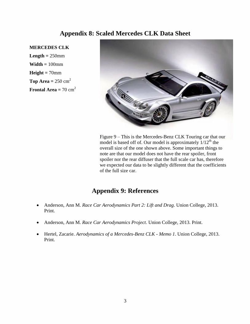
Appendix 8: Scaled Mercedes CLK Data Sheet
MERCEDES CLK
Length = 250mm
Width = 100mm
Height = 70mm
Top Area = 250 cm2
Frontal Area = 70 cm2
Appendix 9: References
Anderson, Ann M. Race Car Aerodynamics Part 2: Lift and Drag. Union College, 2013.
Print.
Anderson, Ann M. Race Car Aerodynamics Project. Union College, 2013. Print.
Hertel, Zacarie. Aerodynamics of a Mercedes-Benz CLK - Memo 1. Union College, 2013.
Print.
Figure 9 – This is the Mercedes-Benz CLK Touring car that our
model is based off of. Our model is approximately 1/12th
the
overall size of the one shown above. Some important things to
note are that our model does not have the rear spoiler, front
spoiler nor the rear diffuser that the full scale car has, therefore
we expected our data to be slightly different that the coefficients
of the full size car.