Draft - University of Toronto T-Space · Draft 1 Framework to assess the pseudo-static approach for the seismic stability of clayey slopes Mourad Karray a, Mahmoud N. Hussien, Marie-Christine

Draft

Framework to assess the pseudo-static approach for the

seismic stability of clayey slopes

Journal: Canadian Geotechnical Journal

Manuscript ID cgj-2017-0383.R1

Manuscript Type: Article

Date Submitted by the Author: 20-Jan-2018

Complete List of Authors: Karray, Mourad; Universite de Sherbrooke, Génie Civil Hussien, Mahmoud; Assiut University, Civil Engineering; Sherbrooke University, Civil Engineering Delisle, Marie-Christine; Ministère des Transports , de la Mobilité Durable et de l’Électrification des Transports Ledoux, Catherine; Ministère des Transports , de la Mobilité Durable et de l’Électrification des Transports

Is the invited manuscript for consideration in a Special

Issue? : N/A

Keyword: pseudo-static, cohesive soil, factor of safety, finite differences, failure surface.

https://mc06.manuscriptcentral.com/cgj-pubs

Canadian Geotechnical Journal

Draft

1

Framework to assess the pseudo-static approach for the seismic stability of clayey slopes

Mourad Karraya, Mahmoud N. Hussiena, Marie-Christine Delisleb, Catherine Ledouxb aDepartment of Civil Engineering, Université de Sherbrooke, Sherbrooke, Québec, Canada b Ministère des Transports, de la Mobilité Durable et de l’Électrification des Transports du Québec, Québec City, Québec, Canada Mourad Karray1. Department of Civil Engineering, Université de Sherbrooke, Sherbrooke, Québec, Canada, [email protected]

Mahmoud N. Hussien. Department of Civil Engineering, Faculty of Engineering, Université de Sherbrooke, Sherbrooke, QC, Canada, [email protected]; Department of Civil Engineering, Faculty of Engineering, Assiut University, Assiut, Egypt, [email protected] Marie-Christine Delisle. Ministère des Transports, de la Mobilité Durable et de l’Électrification des Transports du Québec, Québec, Canada, [email protected] Catherine Ledoux. Ministère des Transports, de la Mobilité Durable et de l’Électrification des Transports du Québec, Québec, Canada, [email protected] 1 Corresponding author Mourad Karray, ing., Ph.D. Professor, Department of Civil Engineering, Université de Sherbrooke, Sherbrooke (Québec) J1K 2R1, Canada Tel.: (819) 821-8000 (62120) Fax: (819) 821-7974 E-mail: [email protected]

Page 1 of 43



Draft

2

Abstract

Approaches commonly used to assess the seismic stability of slopes range from the relatively simple pseudo-static method to

more complicated nonlinear numerical methods, e.g. finite element (FE) and finite difference (FD). The pseudo-static

method, in particular, is widely used in practice as it is inexpensive and substantially less time consuming compared to the

much more rigorous numerical methods. However, the pseudo-static method is widely criticized since it ignores the effects

of the earthquake on the shear strength of the slope material and the seismic response of the slope. Hence, some researchers

recommend its use only in slopes composed of cohesive materials that do not develop significant pore pressures or that lose

less than about 15% of their peak shear strength during earthquake shaking. However, the use of the pseudo-static method in

these soils is also problematic as clayey slopes generally fail in pseudo-static stability analyses (i.e., factors of safety is less

than 1) and the failure surface is completely predominated by the thickness of the clayey layer in the slope or foundation.

The reliability of the pseudo-static method in natural clayey slopes is examined here based on rigorous numerical

simulations with FLAC. The numerical results are compared and verified using available static and dynamic 1-g laboratory

tests. This article then addresses some of the crude assumptions of the pseudo-static method and provides practical

suggestions to be applied to refine the outcomes of pseudo-static analyses not only in terms of the computed safety factors

but also in the prediction of the failure surface through the consideration of additional aspects of the dynamic responses of

the clayey slopes.

Keywords: pseudo-static; clay slopes; factor of safety; finite differences; failure surface. Résumé Les approches couramment utilisées pour évaluer la stabilité sismique des pentes vont de la méthode pseudo-statique,

relativement simple, à des méthodes numériques non linéaires plus compliquées, par ex. élément fini (FE) et différence finie

(FD). La méthode pseudo-statique, en particulier, est largement utilisée dans la pratique car elle est simple et demande

beaucoup moins de temps de calcul que les méthodes numériques beaucoup plus rigoureuses. Cependant, la méthode

pseudo-statique est largement critiquée car elle ignore les effets du séisme sur la résistance au cisaillement du matériau de la

pente ainsi que sa réponse dynamique. Par conséquent, certains chercheurs recommandent son utilisation uniquement dans

les pentes composées de matériaux cohésifs qui ne développent pas de pressions interstitielles significatives ou qui perdent

moins qu'environ 15% de leur résistance au cisaillement lors d'un tremblement de terre. Cependant, l'utilisation de la

méthode pseudo-statique dans ces sols est également problématique car les pentes argileuses ruptures généralement dans les

analyses de stabilité pseudo-statique (ie, les facteurs de sécurité sont inférieurs à 1) et la surface de rupture est complètement

dominée par l'épaisseur des couches argileuse dans la pente ou la fondation. La fiabilité de la méthode pseudo-statique dans

les pentes argileuses naturelles est étudiée dans cet article à l’aide de simulations numériques rigoureuses avec FLAC. Les

résultats numériques sont comparés et vérifiés à l'aide d’essais de laboratoire statiques et dynamiques en 1 g disponibles dans

la littérature. Cet article aborde ensuite certaines hypothèses grossières de la méthode pseudo-statique et fournit des

suggestions pratiques à appliquer pour raffiner les résultats des analyses pseudo-statiques non seulement en termes de

facteurs de sécurité calculés, mais aussi dans la prédiction de la surface de rupture à travers la prise en compte d'aspects

supplémentaires des réponses dynamiques des pentes argileuses.

Keywords: pseudo-statique; pentes argileuses; coefficient de sécurité; différences finies; surface de rupture.

Page 2 of 43



Draft

3

Introduction

The states of natural and engineered slopes vary from marginally stable to very stable with

respect to failure depending on their material, geometric, geologic characteristics as well as

the geotechnical conditions. Earthquake-induced ground shaking creates alternating inertia

forces within the slope and, possibly, significant reduction of shear strength and stiffness of

the slope material (Bray 2007; Kramer 1996). Depending on the predominance of these

effects, seismic slope instabilities can be categorized as “inertial”, “weakening” or combined

“inertial-weakening” instabilities (Kramer 1996; Biondi et al. 2002). In fact, a reliable

evaluation of the seismic stability of slopes, considering these effects, is very important since

several slope stability failures have caused by moderate to large magnitude earthquakes. For

example, the 1920 Haiyuan, the 1964 Alaska, the 1988 Saguenay, and the 2011 Tohoku

Pacific earthquakes caused slope failures that resulted in extensive damage to lifeline systems

and transportation networks (Youd 1978; Tiwari et al. 2013).

Procedures commonly used to assess the stability of slopes during earthquakes range from

the relatively simple pseudo-static method (Terzaghi 1950) to much more sophisticated

nonlinear numerical methods, such as finite element (FE) or finite differences (FD)

simulations (Mizuno and Chen 1982; Daddazio et al. 1987). Since the mid-1960s, most

slopes have been analyzed using the pseudo-static method, an extension of static slope

stability analysis in which the effects of an earthquake are approximated by a spatially

constant horizontal acceleration applied to the geometric model. The stability of the slope is

then evaluated using the method of slices and limit equilibrium to determine a critical failure

surface and a factor of security. The assumption of a constant horizontal acceleration within

the model is a crude approximation especially in slopes with relatively great heights as both

field and laboratory observations have demonstrated that the seismic response (i.e. the

Page 3 of 43



Draft

4

applied horizontal accelerations) varies with height (Duncan et al. 2014; Hynes-Griffin and

Franklin 1984). The method also assumes that the shear strength of the soil within a slope

remains essentially constant and the slope deformations are caused only by the inertial forces

induced by earthquake shaking (it does not account for the potential reduction of shear

strength and stiffness of the slope material due to the development of shear strains during

earthquake shaking). This would be relatively true in cases where there is no significant shear

strength loss during seismic shaking, such as in the case of cohesive soils that do not develop

appreciable excess pore pressures or that lose less than about 15% of their strength during

earthquake shaking. Duncan et al. (2014) indicated that a 15% reduction in clay strength

during shaking can be compensated for by the expected increase in strength (between 20 to

50%) during undrained loading at the rates imposed by earthquakes. However, the use of the

pseudo-static method in these situations is also problematic as the method typically indicates

failure for clayey slopes (i.e. produces factors of safety less than 1) regardless of the actual

stability of the slope and the resulting failure surface is determined by the thickness of the

clayey layer within the slope of foundation, which may not be the case. Moreover, the results

of the pseudo-static analyses are highly dependent on the selected value of the pseudo-

seismic coefficient, kh, which is used to apply a constant horizontal acceleration to the model.

As noted, the representation of earthquake effects by constant acceleration is a crude

approximation and conservative: it assumes that the resulting earthquake-induced forces are

constant and act only in the direction of instability (Jibson 2011).

Rigorous FE or FD numerical analyses using advanced constitutive soil models can

provide direct and salient evaluations of seismic slope stability since they can account for the

interrelated effects of both inertial forces and weakening during shaking. However, they are

much more complex and require significant computational resources, and consequently are

rarely conducted in engineering practice. As a result, force-based (pseudo-static) and

Page 4 of 43



Draft

5

displacement-based (Newmark-type or sliding block; Newmark 1965) methods, despite their

considerable deficiencies, remain in widespread use in engineering practice and research.

Nevertheless, the pseudo-static method could be transformed into a reliable tool for the

evaluation of the seismic stability of clayey slopes provided it can be properly calibrated

using adequate case histories and physical models and can be shown to be in agreement with

rigorous numerical simulations for a wide range of earthquake characteristics and ground

conditions. In structural engineering, properly calibrated simplified procedures are an

essential feature of seismic structural design and are the basis of many code regulations.

However, in geotechnical engineering, simplified procedures such as the pseudo-static

method have not been refined to a level such that they can be applied to clayey slopes with

adequate confidence. They, therefore, should be continually evaluated, validated, and

improved with case histories, small to large-scale physical models and parametric numerical

simulations. The attractive features of the pseudo-static method, in particular its basis in the

limit equilibrium method, routinely used in geotechnical engineering, make it worth the effort

necessary to improve it. In an attempt of doing so, this article closely examines the reliability

of the pseudo-static method in natural clayey slopes and addresses some of the crude

assumptions in its implementation based on a rigorous finite difference modeling using the

two-dimensional computer code FLAC (Itasca 2007). This article then provides some useful

recommendations for the implementation of the pseudo-static method in a manner that

considers the seismic response of the slope in the determination of the critical factor of safety

and location of the corresponding failure surface. Special concern has been devoted in this

article to validate the adopted numerical model using available static and dynamic 1-g

laboratory physical models.

Numerical simulations

Page 5 of 43



Draft

6

The two-dimensional explicit finite difference program FLAC (Itasca 2007) was employed to

evaluate the static and dynamic performance of two homogeneous, 10-m-high clay slopes

with inclinations of 1.75H:1V and 3H:1V, underlain by 20-meter-thick homogeneous clay

foundation and then by a rigid bedrock. The slopes were analyzed statically, pseudo-

statically, and dynamically. Figure 1a shows the basic characteristics (i.e., dimension,

boundaries, and meshing) of the slopes. Quiet lateral boundaries were set away from the

region of interest (near the slope) so that reflected artificial waves were sufficiently damped

and their influence in the slope response was minimized. To determine an adequate width for

the model, preliminary seismic analyses using Synthetic 1 and 2 input motions (Atkinson

2009) were carried out on slope models with widths ranging from 70 m to 960 m. The results

of these analyses are portrayed in Figs. 1b and 1c. In particular, Fig. 1b shows the variation of

the difference between a reference displacement and the maximum horizontal displacement

of the slope toe versus the model width normalized by the slope height (10 m). The reference

displacement is defined here as the maximum horizontal displacement of the slope toe in the

widest model considered (i.e., mesh width equal to 960 m). The analyses were conducted for

different undrained shear strengths (reduction factors, RF, ranging from 1.0 to 1.4 were

considered). The corresponding maximum horizontal displacements of the slope toe are

plotted against the RF in Fig. 1c for different model widths. The displacement-RF curve from

static slope stability is plotted as a reference. Fig. 1b indicates that the change in the horizontal

displacement of the slope toe becomes insignificant a model width of 320 m, and Fig. 1c

confirms that adopting a width of 320 m produces a displacement-RF curve identical to that of

960-m wide model. Quadrilateral soil elements were used since they are less prone to strain

concentration and the mesh extended a horizontal distance of 150 m from both the toe and the

crest of the slope as shown in Fig. 1a.

Page 6 of 43



Draft

7

The simulations were performed in two stages. In the first stage the slope and

foundation soils were represented by the elastic constitutive model implemented in FLAC

and in situ stresses were developed in the model due to gravity. Following this phase, the

strains and displacements within the model were reset to zero. In the second stage, the soils

were represented using the Mohr-Coulomb model as implemented in FLAC. In this stage, the

model was charged by external static or dynamic (an earthquake ground motion) loads. For

the first phase and the static second phase simulations, the mechanical boundary conditions

consisted of horizontal fixity on both sides of the model and horizontal and vertical fixity on

the bottom of the model. In the second phase dynamic simulations, quiet boundary conditions

were applied on the sides to avoid spurious wave reflection and thus simulate the effect of an

infinite elastic medium. The height of the elements affects the transmission of high frequency

shear waves. For this reason, the height of the elements was limited to a maximum height, h,

calculated with (Matthees and Magiera 1982):

max

1

5sV

hf

′≤

(1)

where maxf is the highest excitation frequency used in the analyses, maxf of 10 Hz and sV ′ is

the shear wave velocity expected after the degradation of the shear modulus, G, due to the

developed shear strain and can be related to the initial shear wave velocity sV by:

2

s

max s

G 1

10

V

G V

′= =

(2)

where 1/10 is a typical reduction factor of the shear modulus in a range of 1–10% on the

strain dependent shear modulus curve.

The slope and the foundation were sub-divided into 1-m-thick sub-layers with

constant properties assigned to each sub-layer. The parameters of the Mohr-Coulomb model

are the density, ρ, the cohesion, c, the friction angle, φ, the elastic modulus, E, and the

Page 7 of 43



Draft

8

Poisson's ratio, ν. A Poisson's ratio of 0.45 was used assuming undrained loading.

Accordingly, a friction angle of 0 was used and the cohesion represented the undrained shear

strength, Su. The Su of the slopes was assumed to be 25 kPa at the surface (top of the slope)

and to increase at a rate of 1.5 kPa/m with depth. This relatively low-rate increase of Su with

depth was expected to induce deeper failure surfaces and corresponds to an unfavorable

situation. The maximum shear modulus, Gmax of the soil were evaluated according to the

value of the undrained shear strength, Su (or Cu) following the correlations suggested by

Locat and Beauséjour (1987):

1.05max 0.379= uG C (3)

The shear wave velocity, Vs of the soil was determined based on Gmax from the elastic

relationship between the Gmax and Vs; 2

max sG Vρ= , where ρ is the soil density. Input

parameters of the Mohr-Coulomb model used in this study are listed in Table 1. The

parameters of the elastic model that was used in the first phase of the simulations are the

elastic modulus and the Poisson’s ratio. The values used were the same as those of the second

phase.

In the dynamic simulations, the shear modulus of the soils were degraded using the

constitutive model SIG4 (Itasca 2007) capped by the Mohr-Coulomb failure criteria

following the experimental curves suggested by Vucetic and Dobry (1991) for a plasticity

index, PI, of 30. The fitted parameters of the SIG4 model are listed in Table 1. Additionally, a

Rayleigh damping ratio of 0.0015 was used to ensure stability of the numerical solution

process at low strain levels.

Validation of the numerical method based on physical modelling

Page 8 of 43



Draft

9

Prior to the main part of this study, the validity of the numerical method was verified by

simulation of the monotonic (static) and dynamic responses of clayey slopes from the 1-g

physical model testing conducted by Ozkahriman (2009). The physical tests were performed

in a 2.03 × 1.22 × 0.60 m rigid Plexiglass box bolted to a shaking table. Three clayey slope

models (static models S1, S2, and S3) were constructed and then tested to study the stability

of slope under static loading conditions. Three other models (dynamic models D1, D2, and

D3) were built and then shaken to investigate the stability of the slope under dynamic loading

conditions. These models typically consisted of two soil zones: an upper soft clay layer

underlain by a stiffer clay layer that was in contact with the front and rear walls of the box.

The geometries of the slope models are given in Table 2. The largest models (S1 and D1) of

the two sets of experiments were considered as the “prototype" earth structures. For the two

smaller models, geometry, strength, low-strain properties (shear modulus), and frequency

content of the input motions were adjusted by applying the laws of similitude (Iai, 1989) to

reflect their reduced scales. The selected scaling factors (λ) for smallest and middle model

were 2.5 and 1.43, respectively. Assuming a geometric scaling factor (λ) of 22, the models

(S1 and D1) can be said to represent a 45o, 12 m height of soft clay embankment having a

constraint undrained shear strength of 75 kPa and shear wave velocity of 45 m/sec. The

Model S0 in Table 2 was a duplicate model of S1 to evaluate the repeatability of

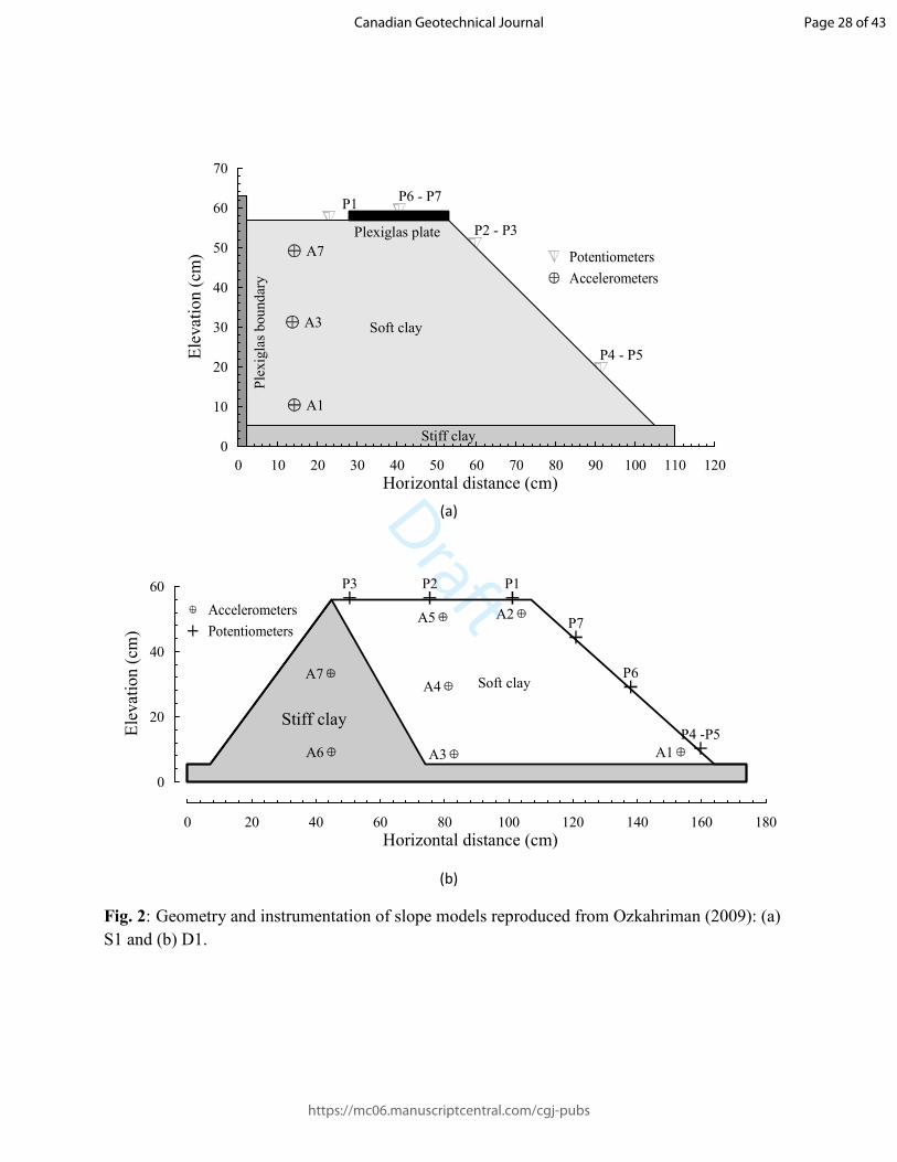
experimentations. Detailed geometries and the instrumentation of models S1 and D1 are

respectively shown in Fig. 2a and Fig. 2b. The dynamic responses of the model were

measured at different depths using capacitive spring mass-based miniature accelerometers

(i.e. A1 to A7). Surface displacements were measured using either 50-mm or 100-mm-range

linear motion potentiometers (i.e. P1 to P7) with a linearity of less than +/- 1% and a

resolution that is reported as “essentially infinite”. Detailed descriptions of the

instrumentation can be found in (Ozkahriman 2009).

Page 9 of 43



Draft

10

The models were constructed using a kaolinite-bentonite “model clay” (kaolinite to

bentonite ratio of 1:3) originally developed by Seed and Clough (1963) for use at the

University of California, Berkeley in physical modeling to simulate the stress-strain behavior

of the San Francisco Bay Mud characterized by a low rate of consolidation and a Vs of 120-

180 m/sec. Another important characteristic of the mixture is that its undrained shear strength

is determined by its water content (Wartman. and Riemer 2002), thus the undrained strength

can be controlled. The clay has liquid (LL) and plastic (PL) limits of 120 and 25,

respectively, and a plasticity index (PI) of 95 (Ozkahriman 2009).

Prior to model construction, the geometry of the slope and the instrumentation layout were

marked on the Plexiglas walls to provide guidance. The stiff base layer was placed first,

followed by the upper layer of soft clay, and the accelerometers and potentiometers were

placed in the models at the predetermined locations shown in Fig. 2. Each handful of clay

was carefully "worked" into the layer below to ensure uniformity and prevent formation of

any construction-influenced preferential shear surfaces. Once model construction was

completed, surface elevations were measured, and they were found to be essentially uniform

across the width of the model slope typically varying by no more than several millimeters

(Ozkahriman 2009).

As shown in Fig. 2a, the static models were subjected to a surface loads applied by means

of a 2.5-cm-thick Plexiglas footing on the crest of the slope. A load of a maximum magnitude

of 900 N was gradually applied using a hand crank at a constant rate of 360 N/min. The

dynamic models were subjected to a suite of ground motions including synthetic (frequency

sweeps and sine waves) and recorded earthquake motions with varied frequency content,

duration, and amplitude. The frequency sweep motions consisted of a four-second ramping

windows at the beginning and at the end of the full amplitude motion. The input frequency

linearly increased from 5.4 Hz to 12.5 Hz during the 20-second duration of the motion. The

Page 10 of 43



Draft

11

models were shaken with low amplitude (0.03g < PGA < 0.08g) sine sweeps to provide

information on the dynamic characteristics of the models before moderate-to-high amplitude

sine pulses and the recorded 1989 Loma Prieta earthquake motion at Redwood City (RWC)

seismograph station (details are tabulated Table 3) have been applied. These later motions

induced permanent deformation in the models (Ozkahriman 2009).

The responses of the S1 and D1 models were simulated numerically using the numerical

model presented in the previous section. The grid was built sequentially to model the actual

construction sequence of the physical models. The soil was modeled as an elastic material

during the construction process to prevent any localized construction-induced rupture zones.

After the simulation of staged of construction, the strains and displacements of the model

were reset to zero and the Mohr-Coulomb model was assigned to the soil. The sigmoidal

(SIG4) model was adopted to fit the shear modulus degradation curves of the clay during

dynamic loading based on the experimental curves suggested by Vucetic and Dobry (1991)

for a PI of 100%. The parameters used to numerically simulate the physical models are given

in Table 4. The boundary conditions (e.g. mechanical fixity) and static and dynamic load

application in the numerical simulations were the same as those used in the physical models.

The post-failure localized shear surfaces at the middle sections of physical models S0 and

S1 are plotted on the corresponding numerically simulated deformed mesh in Fig. 3a. In Fig.

3b, the failure surfaces of physical models S2 and S3 were respectively scaled by 1.43 and

2.5 times (i.e., geometric scaling factor, λ, in Table 2) relative to that of S1 model. Figs. 3a

and 3b show that the observed post-test profiles are generally similar for all tested slope

models (S0, S1, S2, and S3) though the behavior near the toe of S0 and S1 models differ

somewhat from that of the other models (S2 and S3) in which the rotational shear surfaces

pass through the toes of the slopes. Furthermore, Fig. 3a shows that the internal shear surface

of the model S0 is somewhat shallower than the model S1, which can be interpreted through

Page 11 of 43



Draft

12

a close examination of the vertical deformation at the top of slope models S1 and S0 beneath

the Plexiglas plate. As shown in Fig. 3a, the loaded plate in the first case S1 has a relatively

non-uniform vertical deformation, as the inner vertical settlement is significantly greater than

the outer one. It seems that the load control of the Plexiglas plate is improved when the test

was repeated (the second model S0) resulting in a more uniform foundation settlement. In

other words, the unbalanced vertical deformation of the loaded plate generated in the model

S1 resulted in a deeper localized shear surface, rationalizing the differences in the internal

shear surfaces presented in Fig. 3a. To cope with these uncertainties in the control of the

loaded plate translation and rocking deformations, two cases of numerical simulation have

been considered. In the first case (Case 1), the lateral displacement of the loaded plate was

permitted and in the second case (Case 2), the lateral motion of the plate was prevented. The

computed failure surface of the first case was found to fall within the upper and lower failure

surfaces observed in S0 and S1 physical tests shown in Fig. 3a, while that of the second case

coincides with the observed post-test profiles of slope models S2 and S3 presented in Fig. 3b.

Measured and computed load-deformation responses of the Plexiglas plate at P6 in model

S1 are presented in Fig. 4a. The observed load-deformation curves of other tests (S2 and S3)

are also presented in Fig. 4a for comparison. The curves presented in Fig. 4a reflect the real

and the simulated strain-softening nature of the model clay. Although the current numerical

model doesn’t completely simulate the gradual reduction in the clay strength after failure

(i.e., after the peak resistance) as it utilized the elastic-perfectly plastic Mohr-Coulomb

model, the computed pre-failure load-deformation responses are generally in good agreement

with the measured curves. The measured and the computed horizontal displacements at

potentiometers P3 and P5 are respectively plotted as functions of the vertical displacement at

P6 in Figs 4b and 4c. The numerical prediction of the horizontal displacement when the plate

is not allowed to displace horizontally (case 2) is generally greater than the experimental

Page 12 of 43



Draft

13

responses at P3 (Fig. 4b) but it is very close to the response of the experimental model S1

(Fig. 4c). When the horizontal displacement of the plate is allowed (Case 1), the numerical

results are significantly improved and become closer to the experimental results. Even if the

numerical prediction generally overestimates the data at the lower vertical displacements and

provides an underestimation at greater vertical displacements, they can be viewed as an

average estimation of the experimental results.

It should be noted that the observed localization of the shear surface shown in Fig. 3a and

the load-deformation curves in Fig. 4a are more similar to a bearing capacity problem (for a

shallow foundation near a slope) than that to a pure slope stability problem reflecting the

response of the experimental model to the type of the load applied. Simulating these

experimental static results, however, constitutes one of the first and important stages of the

validation process of the numerical procedure adopted in this study and serves to ensure the

applicability of the numerical procedure to predict soil deformations under static loading

before going further and examining its pertinence in modeling the more complicated dynamic

slope stability problem.

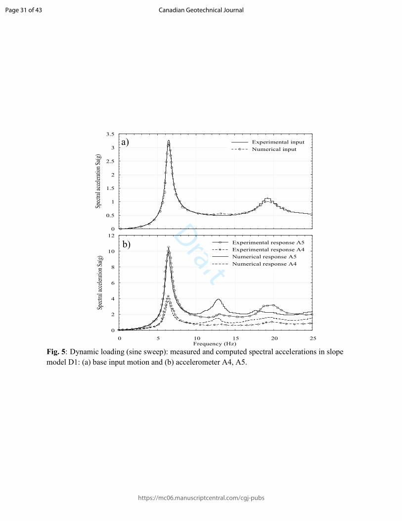
The dynamic response of Model D1 during shaking table test subjected to the sine pulse

shown in Table 3 was also simulated numerically. The recorded time history at an

accelerometer attached to shaking table, the input motion used, was baseline corrected before

using it in the numerical analysis. Figure 5a shows the spectral accelerations used in the

physical modeling and numerical simulations. Figure 5b presents the measured and the

computed responses of accelerometers A4 and A5 shown in Fig. 2b. Figure 5b shows that the

FLAC simulation of the dynamic response of the slope model is in good agreement with the

shaking table measurements, and the shape of the predicted spectral acceleration curves are

very similar to the measured curves.

Page 13 of 43



Draft

14

Figures 6a and 6b, respectively, present comparisons between the measured and the

computed spectral accelerations of the accelerometers A4 and A5 during a ground motion

equivalent to that recorded at the Redwood City location during the 1989 Loma Prieta

earthquake. Two different numerical simulations with and without pre-shaking (using the low

amplitude motions mentioned above) were performed and the results of both analyses are

presented in Fig. 6. Figure 6 shows that the numerical spectral accelerations at both locations

(A4 and A5) match well the measurements from the physical models, specifically, the shapes

of the simulated spectral acceleration curves are in general in good agreement with the

measured curves from physical modeling. The measured and the computed overall response

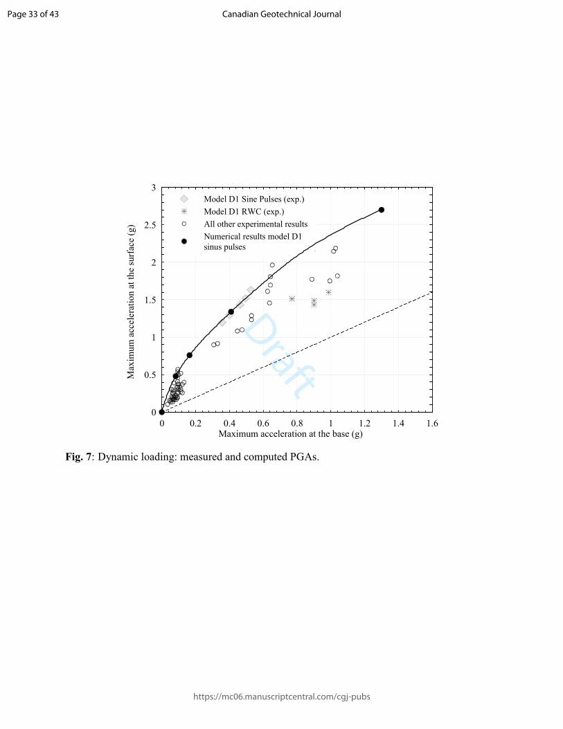
during dynamic tests are further represented in Fig. 7 in terms of peak ground accelerations

(PGAs) at the surface as functions of the maximum input accelerations. Figure 7 indicates

that similar trends can be seen between computed and measured amplification ratios and thus

numerical simulations produce PGAs that match well those measured in the shaking table

tests. Also, the computed and the measured post-test profiles and failure surfaces due to the

Redwood city ground motion are presented in Fig. 8, and these surfaces are generally similar.

Figure 8 shows also that the deformations are distributed along the height of the model and

localized along a single failure surface indicated by deep rotational and translational

displacements passing through toe of the slopes which is well predicted in simulation by the

localization of shear strain close to the base (toe) of soft clay layers and at the interface

between the soft and stiff clay layers.

The comparative results presented in Figs. 3 to 8 indicates that the adopted numerical

model could be used to simulate the static and dynamic responses of clayey slopes such as

those presented here.

Page 14 of 43



Draft

15

Results of static, pseudo-static and dynamic analyses The basic condition for static or dynamic stability of slopes is that the mobilized shear

resistance (capacity) must be greater than the applied shear force (demand). A slope could be

brought to the brink of instability either by a reduction of the shear resistance of the soil on

some potential failure surface or by an increase in the imposed static and dynamic loads. In

this study, a unified framework has been adopted to access the stability of slopes under static

and dynamic loadings. This approach is used in all the static, pseudo-static and dynamic

analyses and consists of a determination of a reduction factor applied to the resistance (Su) of

the cohesive soil that leads to the slope failure (Karray et al. 2001). In other words, the main

component of the framework is a systematic search for the value of the reduction factor (i.e.,

the factor of safety) that will cause the slope to fail. For a given static, pseudo-static, or

dynamic analysis, the calculations were repeated several times with different values of soil

shear strength and the relative horizontal displacement between two arbitrary points

(typically, at the slope toe and the corresponding point at the bedrock) was noted and plotted

as a function of the applied strength reduction factor. The equivalent factor of safety can be

then determined from this plot as the reduction factor corresponding to the general

plastification (i.e., the significant and sudden increase in the relative horizontal

displacement). Moreover, the formation of the failure surface is also investigated during the

numerical simulations for the shear strength reduction procedure, as the factor of safety is

known to be directly linked to the development of the failure surface.

The static numerical simulations of the clayey slopes considered in this study were

performed using the undrained shear strength parameters and the above procedure was used

to obtain the factors of safety and the corresponding failure surfaces. There was no initial

assumption concerning the shape and location of the failure surface. It is noted that the static

stability of a slope doesn’t ensure its stability under dynamic conditions. However, the static

Page 15 of 43



Draft

16

analyses were carried out in this study to: (i) assess the slope stability under static conditions;

(ii) compare these results with the subsequent pseudo-static and dynamic analyses; and (iii)

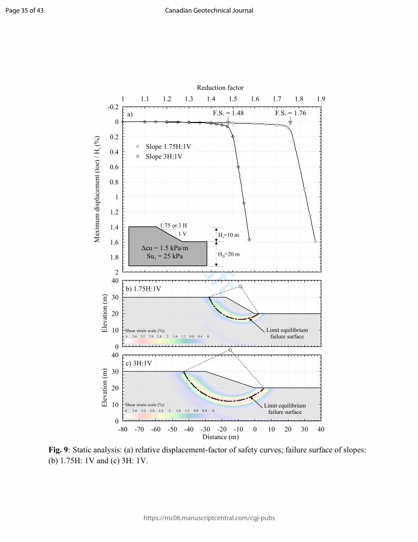
evaluate the procedure adopted for estimating the safety factors. The height-normalized

relative displacement (an approximation of the soil shear strain, γ%)-reduction factor curves

of the static analyses are presented in Fig. 9a, while the corresponding failure surfaces are

plotted in Figs. 9b and 9c for the 1.75H:1V and 3H:1V slopes, respectively. Figure 9a shows

that the safety factors obtained for the 1.75H:1V and 3H:1V slopes, respectively, are 1.48 and

1.76. These values agree well with those estimated using well-known limit equilibrium

methods such as Bishop’s modified (Bishop 1955), Spencer (Spencer 1967), Morgenstern-

Price (Morgenstern, and Price 1965), and Fredlund-Krahn (GLE) (Fredlund and Krahn 1977)

as presented in Table 5. Figures 9b and 9c, respectively portray the corresponding yielded

zones obtained from FLAC analyses for 1.75H:1V and 3H:1V slopes. The slip surfaces

determined from the limit equilibrium analyses are also reported on Figs. 9b and 9c, and they

generally fall within or close to the plastified zones determined by the current FD model.

The pseudo-static analyses were conducted using the same conditions as the static

analyses and the corresponding reduction factors-normalized displacement curves are plotted

in Fig. 10a. A pseudo-static coefficient of 0.15 was used to calculate the equivalent horizontal

inertial forces. Because the prime objective of this work is to assess the seismic stability of

clayey slopes in the Québec city region, the value of the pseudo-static coefficient (0.15) was

selected following the recommendation of the Centre d’expertise hydrique du Québec (Centre

d’expertise hydrique du Québec 2013). This value corresponds to about half of the maximum

acceleration on rock for this region. Figure 10a shows that the safety factors obtained for the

1.75H:1V and 3H:1V slopes are almost the same of 0.95 and they are successfully compared

to those estimated using typical limit equilibrium methods (Bishop 1955; Fredlund and Krahn

1977) as presented in Table 5. Figures 10b and 10c respectively portray the corresponding

Page 16 of 43



Draft

17

yielded zones obtained from FLAC analyses for the 1.75H:1V and 3H:1V slopes. The slip

surfaces determined from typical static limit equilibrium analyses are also reported in Figs.

10b and 10c. In both cases, the failure surface obtained from the pseudo-static analysis is

very deep and passes close to bedrock. There is a significant difference between these

surfaces and those estimated from the static limit equilibrium analyses.

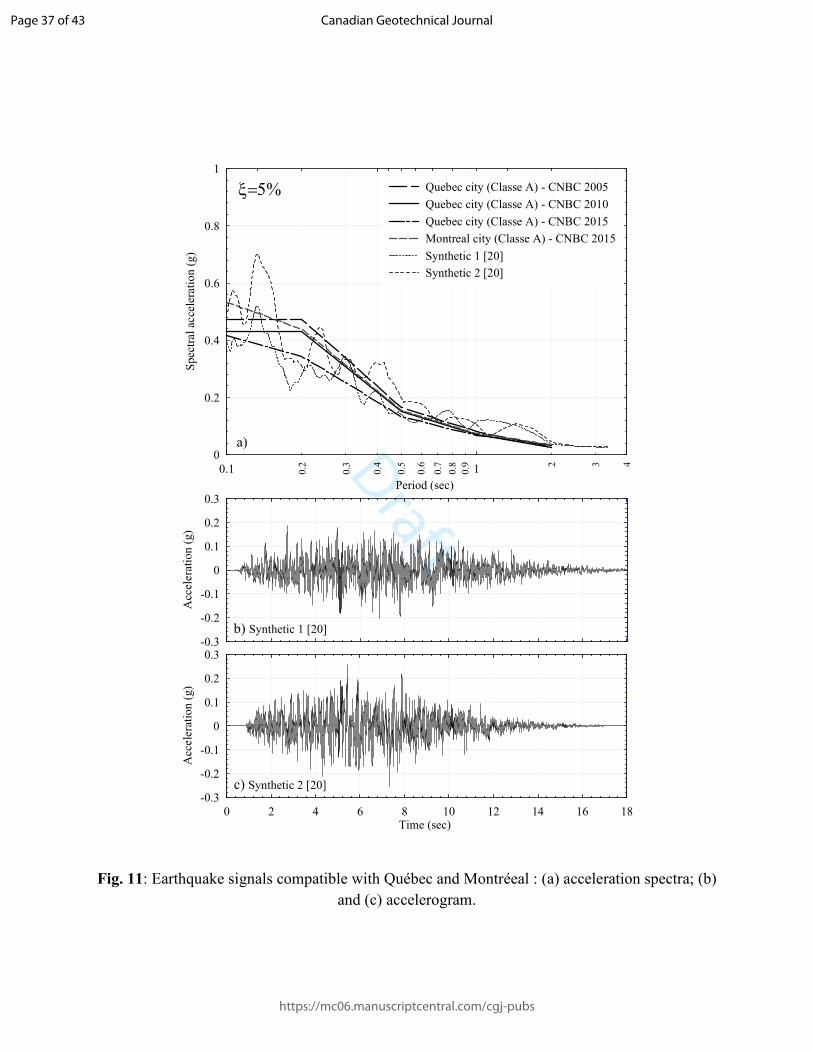
In the same manner, the dynamic analyses were conducted using Synthetic 1 and 2 input

motions (Atkinson 2009) compatible with the seismicity of the region of Quebec city, which

are respectively shown in Fig. 11b and 11c. They were selected because the resulting

response spectra (Fig. 11a) are compatible with that given by the CNBC 2005, 2010, and

2015 for Quebec and Montreal for site class A sites (hard rock). Before discussing the results

of the seismic analyses, recall that the seismic analysis of slopes is rather complex and

requires consideration of the effect of the dynamic stresses induced by the earthquake

(inertial effects) as well as the potential for strength loss within the soil (weakening effects).

In the former, the shear strength remains relatively constant, but strains develop due to

temporary exceedance of the capacity. In the latter, the earthquake may induce soil strength

loss, reducing the capacity, and strains develop due to exceedance of the reduced capacity. In

the current analyses, strength loss was considered. However, the analyses were conducted

considering typical degradation of the shear modulus and an increase in damping with

increasing shear strain. This assumption is probably acceptable in clayey slopes that do not

develop significant dynamic pore pressures or lose more than about 15% of their peak shear

strength during earthquake shaking as reported by Kramer (1996) or can be inferred from the

results presented by Matasovic and Vucetic (1995); and Vucetic and Dobry (1988). This

assumption is compatible with the pseudo-static method implemented using limit

equilibrium.

Page 17 of 43



Draft

18

The computed normalized displacement-reduction factor curves of both 1.75H:1V and

3H:1V slopes under Synthetic 1 and 2 input motions (Atkinson, 20) are plotted in Fig. 12a.

The computed factors of safety of the 1.75H:1V under Synthetic 1 and 2 input motions are

1.17 and 1.25, respectively. The corresponding factors of safety of the 3H:1V are 1.35 and

1.45. It can be noticed from Fig. 12a that the change in the displacement-reduction factor

curve is relatively smooth compared to the static and the pseudo-static curves. Thus, the

factor of safety is determined in this case by constructing two tangents: one to the first

straight segment of the curve and the other one to the lower straight segment. A bisector is

then drawn intersecting the curve at a point that corresponds to where the failure would

occur. It should be also noticed that these safety factors correspond to a normalized relative

displacement (average shear strain) of 0.2. Figures 12b and 12c, respectively, portray the

corresponding yielded zones obtained from FLAC analyses for the 1.75H:1V and 3H:1V

slopes. The slip surfaces determined from the static limit equilibrium analyses are also shown

on Figs. 12b and 12c for reference. Figures 12b and 12c indicate there are two potential

failure surfaces due to the dynamic loading. The shallower one rather resembles the slip

circle obtained from the static analysis, and it is very different from the surfaces predicted by

the pseudo-static approach. The deeper failure surface is generated as expected at the

interface between clay and bedrock. Similar failure surfaces have been observed in the

physical test results as presented in Fig. 8. In the case of the 3H:1V slope, the dynamic failure

surface is a bit wider than in the 1.75H:1V slope.

It should be mentioned here that both the clayey slopes considered have been shown to be

stable in static and the dynamic analyses (factors of safety greater than 1) but failed in the

pseudo-static analyses that produced, moreover, unrealistic slip surfaces.

The dynamic numerical analyses conducted in this study could lead to some valuable

information with respect to the fundamental behavior of clayey slopes during earthquakes and

Page 18 of 43



Draft

19

would enrich the current understanding of common assumptions used in the evaluation of

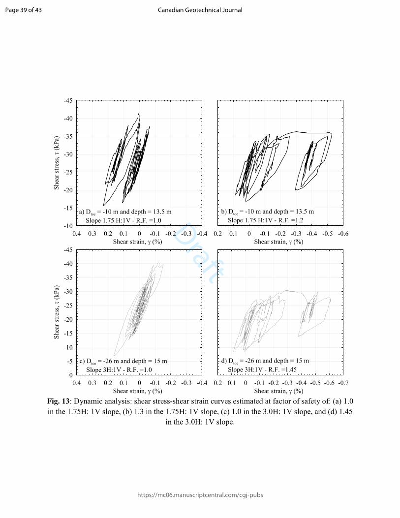
such slopes by the pseudo-static method. For example, Figs. 13a-d depict the shear stress-

shear strain response of the soil at different locations within the slope during the dynamic

analyses of both cases considered. Specifically, Figs. 13a and 13b respectively show the soil

stress-strain loops of a point close to the computed yield zone (Fig. 12b) at a 13-m depth and

a 10-m distance from the slope toe plotted for a reduction factor of 1.0 (i.e., immediately

prior to failure) and 1.2 (i.e., instantly after the failure). Similarly, Figs. 13c and 13d

respectively show the soil stress-strain loops of a point close to the computed yield zone (Fig.

12c) plotted for reduction factors of 1.0 and 1.45. Figs. 13a and 13c (plotted immediately

before the slope failure) show the degradation of the clay stiffness with shear strain. Unlike

the cohesionless soil response to seismic excitation that exhibit a substantial reduction in its

stiffness manifested by a significant rotation of the stress-strain loop towards the horizontal

axis, the clay experiences limited rotation of the stress-strain loop and consequently less

relative reduction in its shear modulus. Immediately after the failure, Figs. 13b and 13d

indicate that a decrease of the soil peak shear resistance (42 kPa in Fig. 13a) to a residual

strength (36 kPa) has been occurred and the difference between the peak and the residual

strength of the soil at the point in question is transferred to the surrounding soil. These

redistributions of stresses may cause the peak strengths in the surrounding soil to be reached

resulting in a progressive growth of the failure zone (i.e., propagation of the failure zone)

until the entire slope become unstable.

Figure 14 shows the spectrum corresponding to the input motion used in the dynamic

analysis versus the design spectrum of Quebec and Montreal provided in the national

building code, CNBC 2015. The spectral accelerations of different points within the slope

model considered are also plotted in Fig. 14. These points are located: (1) on the top of the

slope, 70 m from the crest (upstream); (2) at mid-slope; and (3) at the bottom of the slope, 50

Page 19 of 43



Draft

20

m from the toe. Figure 14 demonstrates that the fundamental period varies from 1.19 sec. at

the top of the slope (1) to 0.72 sec at the bottom of the slope (3) and that the second-mode

periods of the slope converge close to the maximum design spectral acceleration. These

effects are because of geometry and the distribution of the soil properties. Figure 14

demonstrates also that there a substantial amplification of the seismic response around the

fundamental mode of vibration (i.e., period = 1.19 sec) at the surface both at the top and base

of the slope with an average amplification ratio of 3 with respect to the bedrock motion. With

this average amplification, the spectral acceleration at the fundamental mode approaches the

design spectrum. On the other hand, the amplification ratio at the second mode of vibration

can be neglected. The results presented in Fig. 14 could, in part, justify the use of the pseudo-

static method if the design acceleration value is consistent with the fundamental period. In

other words, the earthquake effect could be replaced by an acceleration that acts in the

direction of instability, such as the fundamental mode of vibration. These results also call in

to question the use of a constant acceleration over the entire soil slope as there a substantial

variation of the seismic response at different locations of the slope at the fundamental mode

of vibration.

Recommendations to refine the pseudo-static procedure outcomes

Based on the comparative results of the dynamic and pseudo-static analyses discussed in the

previous section and the literature pertaining to the topic, one of the main simplifying

approximations of the pseudo-static method is that it uses a constant seismic coefficient over

the entire height of the slope. In this study, the authors postulated that using either linear or

segmental variation of the pseudo-static coefficient over the height of the slope in the analysis

of clayey slopes would be a significant improvement. Several numerical analyses with

different variations of the pseudo-static coefficient with depth were conducted and the

Page 20 of 43



Draft

21

authors found that a variation of the seismic coefficient in the hyperbolic form (Eq. 4) would

lead to a significant improvement of the method:

20[1 2( / ) ]h z h tk k z H= + (4)

where khz and kho are the seismic coefficients at any distance z measured from the bedrock

level and at the bedrock (initial value), respectively; Ht is the total height of both the slope

and the deposit. The modified hyperbolic profile of the seismic coefficient could be then

incorporated into numerical slope stability analysis by multiplying the mass of each row of

soil elements in the slope model at a certain depth by the value of the seismic coefficient at

the same elevation, thus obtaining a non-uniform distributed seismic force along the entire

depth of the slope. Figure 15 presents an example of the obtained results. Figure 15a shows

the normalized relative displacement-reduction factor curves obtained from the suggested

pseudo-static analysis at for the 1.75H:1V and 3H:1V slopes under Synthetic 1 and 2 input

motions. For the 1.75H:1V slope, kho values of 0.035 and 0.045 are selected for the pseudo-

static analyses under Synthetic 1 and 2 input motions, respectively. These values lead to

seismic coefficient at the ground surface of 0.105 and 0.135 (these values are relatively close

to the assumed value of the seismic coefficient in conventional pseudo-static procedure

(0.15)). As shown in Fig. 15a, these selected values produce a factor of safety identical to that

obtained from the numerical simulation at similar shear strain of 0.2. On the other hand, the

best safety factors for the 3H:1V slope were been reached at values of seismic coefficients at

the ground surface of 0.081 and 0.105 for Synthetic 1 and 2 motions, respectively. The

corresponding failure surfaces are also improved when the suggested profile of the seismic

coefficient is included in the pseudo-static analysis. Figures 15b and 15c show the slip

surfaces obtained from modified pseudo-static analysis over which the slip surfaces of the

dynamic analysis is plotted in dashed line for the 1.75H:1V and 3H:1V slopes, respectively.

It is observed that the yield surfaces are very similar. Moreover, the deeper failure surface

Page 21 of 43



Draft

22

previously observed in the dynamic analysis of the 3H:1V slope has been appeared in the

suggested pseudo-static analysis, but it is somewhat wider than that in detected in the

numerical analysis.

Conclusions

A close examination of the simplistic assumptions of the conventional pseudo-static method

was conducted through a rigorous framework based on static and dynamic finite difference

simulations conducted using the Mohr-Coulomb constitutive model and the SIG4 shear

modulus reduction and damping model. The numerical modeling was validated using

published data from static and dynamic 1-g physical modeling. Two homogeneous clayey

slopes: 1.75H:1V and 3H:1V overlying a 20-meter thick homogeneous clay foundation layer

underlain by bedrock were analyzed statically, pseudo-statically and dynamically. The results

of these analyses were compared in terms of the estimated factor of safety and the developed

failure surfaces. Based on the comparative results presented in this study, the following

conclusions were made:

1. Generally, the conventional pseudo-static procedure significantly under-estimates the

factor of safety of clayey slopes.

2. The failure surfaces obtained from the pseudo-static analysis are typically very deep

and there are significant differences between those surfaces and the failure surfaces

estimated from numerical simulations.

3. Careful examination of the spectral acceleration ratios of different points within the

slopes based on dynamic numerical simulations show that the assumption of replacing

the earthquake effect by a unidirectional acceleration could be acceptable. However,

the use of a constant acceleration over the entire soil slope mass is a very simple

approximation and overly conservative.

Page 22 of 43



Draft

23

4. The use of a hyperbolic variation of the seismic coefficient with depth would produce

factors of safety and failure surfaces very similar to that obtained from the numerical

simulations and can be readily accomplished in numerical analysis.

Acknowledgements

The authors would like to express their gratitude to le Ministère des Transports, de la

Mobilité Durable et de l’Électrification des Transports for supporting this research. The

authors also want to express their gratitude to Mr. Gilles Grondin and Mr. Denis Lessard who

were the initiators of this research project.

Page 23 of 43



Draft

24

References

Abramson, L.W., Lee, T.S., Sharma, S., and Boyce, G.M. 2002. Slope Stability and Stabilization Methods. vol. 2e. New York: John Wiley & Sons, Inc.

Ambraseys, N.N. 1960. The Seismic Stability of Earth Dam. Second World Conf. Earthq. Eng. Vol. 2, Tokyo, Japan: p. 1345–63.

Atkinson, G.M. 2009. Earthquake time histories compatible with the 2005 National building code of Canada uniform hazard spectrum. Canadian Journal of Civil Engineering, 2009, 36(6): 991-1000, 10.1139/L09-044.

Bishop, A.W. 1955. The use of the Slip Circle in the Stability Analysis of Slopes. Géotechnique 5: 7.

Biondi, G., Cascone, E., and Maugeri, M. 2002. Flow and deformation failure of sandy slopes. Soil Dynamics and Earthquake Engineering 22: 1103–1114.

Bray, J.D. Chapter 14: 2007. Simplified seismic slope displacement procedures.” Proc., Earthquake Geotechnical Engineering, 4th Int. Conf. on Earthquake Geotechnical Engineering—Invited Lectures, K. D. Pitilakis, ed., Vol. 6, Springer, New York, 327–353.

Centre d’expertise hydrique du Québec. 2013. Carte numérique. Available from https://www.cehq.gouv.qc.ca/loisreglements/barrages/reglement/Seismiques_QC_150.pdf.

Daddazio, R.P., Ettouney, M.M., and Sandler, I.S. 1987, Nonlinear dynamic slope stability analysis. Journal of Geotechnical Engineering, ASCE, 113(4): 285–298.

Duncan, J.M., Wright, S.G., and Brandon, T.L. 2014. Soil Strength and Slope Stability. John Wiley & Sons, Inc.

Fredlund, D.G., and Krahn, J. 1977. Comparison of slope stability methods of analysis", Canadian Geotechnical Journal, 14 (3): 429–439.

Houston, S.L., Houston, W.N., and Padilla, J.M. 1987. Microcomputer-Aided Evaluation of Earthquake-Induced Permanent Slope Displacements. Comput Civ Infrastruct Eng; 2:207–22.

Hynes-Griffin, M.E., and Franklin, A.G. 1984. Rationalizing the Seismic Coefficient Method. Miscellaneous Paper No. GL-84-3, U.S. Army Engineer Waterways Experiment Station, Vicksburg, Mississippi.

Iai, S. 1989. Similitude for shaking table test on soil-structure-fluid model in 1-g gravitational field. Soils and Foundations, Vol. 29 (1): 105–118.

Ishihara, K. 1993. Liquefaction and flow failure during earthquakes. Géotechnique 43(3): 351–415.

Itasca 2007. FLAC - Fast Lagrangian Analysis of Continua, Version 6. User’s Manual. Itasca Consulting Group, Inc. Minneapolis, Minnesota, USA.

Jibson, R.W. 2011. Methods for assessing the stability of slopes during earthquakes—a retrospective. Engineering Geology 122, 43–50.

Karray, M., Lefebvre, G., and Touileb, B.N. 2001. A procedure to compare the results of dynamic and Pseudo-Static slope stability analyses. 54th Can. Geotech. Conférence/ 2th Jt. IAH CGS Groundw. Conf., p. 888–93.

Kramer, S.L. 1996. Geotechnical earthquake engineering. USA: Prentice-Hall1.

Locat, J., and Beausejour, N. 1987. Corrélations entre des propriétés mécaniques dynamiques et statiques de sols argileux intacts et traités à la chaux. Can Geotech J; 24:327–34.

Page 24 of 43



Draft

25

Lefebvre, G., Leboeuf, D., and Hornych, P. 1992. Slope failures associated with the Saguenay earthquake, Quebec, Canada. Canadian Geotechnical Journal; 29:117–130.

Matasovic, N., and Vucetic, M. 1995. Generalized cyclic degradation pore pressure generation model for clays. Journal of Geotechnical Engineering, ASCE, 121(1): 33–42.

Matthees, W., and Magiera, G.A. 1982. Sensitivity study of seismic structure-soil-structure interaction problems for nuclear power plants. Nuclear Eng Des; 73(3):343–363.

Meehan, C.L., and Vahedifard, F. 2013. Evaluation of simplified methods for predicting earthquake-induced slope displacements in earth dams and embankments. Engineering Geology, 152: 180–193. doi:10.1016/j.enggeo.2012.10.016.

Mizuno, E., and Chen, W.F. 1982. Plasticity Models for Seismic Analysis of Slopes. Report Number CE-STR-82-2, School of Civil Engineering, Purdue University, West Lafayette, Ind., Jan.

Morgenstern, N.R.; and Price, V. E. 1965. The analysis of the stability of general slip surfaces. Géotechnique, 15 (1): 79–93.

Newmark, N.M. 1965. Effects of earthquakes on dams and embankments. Géotechnique, 15 (2): 139–160.

Ozkahriman, F. 2009. Physical and numerical dynamic response modeling of slopes and embankments. Ph.D thesis, Drexel University.

Seed, H.B., and Clough, R.W. Earthquake Resistance of Sloping Core Dams. Journal of. Soil Mechanics and Foundation Div., ASCE, Vol. 82 (SM2), 1963.

Spencer, E. 1967. A method of analysis of the stability of embankments assuming parallel inter-slice forces. Géotechnique.

Terzaghi, K.1950. Mechanisms of landslides. The Geological Society of America.

Tiwari, B., Wartman, J., and Pradel, D. 2013. Slope stability issues after Mw 9.0 Tohoku Earthquake. Geotechnical Special Publication, Geo-Congress, ASCE; 1594–1601.

Vucetic, M., and Dobry, R. 1991. Effect of Soil Plasticity on Cyclic Response, Journal of Geotechnical Engineering, ASCE, 117(1): 89-107.

Vueetic, M., and Dobry, R. 1988. "Degradation of marine clays under cyclic loading." J. Geotech. Engrg,. ASCE, 114(2), 133-149.

Wartman, J., and Riemer, M. F. 2002. The use of fly ash to alter the geotechnical properties of artificial model clay. In Proc. 1st Int. Conf. on Phy. Model, in Geot., St John's, Canada.

Youd, T.L. 1978. Major cause of earthquake damage in ground failure. Civil Engineering, ASCE, 48(4): 47–51.

Page 25 of 43



Draft

26

Figure captions Fig. 1: Basic characteristics of the slope under investigation, meshing, and associated boundary conditions. Fig. 2: Geometry and instrumentation of slope models reproduced from Ozkahriman (2009): (a) S1 and (b) D1. Fig. 3: Static loading: localized shear surfaces and their corresponding deformed meshes of numerical models: (a) S0, S1 and (b) S2, S3. Fig. 4: Static loading: real and the simulated load-deformation behavior of the slopes. Fig. 5: Dynamic loading (sine sweep): measured and computed spectral accelerations in slope model D1: (a) base input motion and (b) accelerometer A4, A5. Fig. 6: Dynamic loading (Redwood motion): measured and computed spectral accelerations at: (a) A4 and (b) A5. Fig. 7: Dynamic loading: measured and computed PGAs. Fig. 8: Dynamic loading (Redwood motion): measured and computed post-test profiles and failure surfaces. Fig. 9: Static analysis: (a) relative displacement-factor of safety curves; failure surface of slopes: (b) 1.75H:1V and (c) 3H:1V. Fig. 10: Pseudo-static analysis: (a) relative displacement-factor of safety curves; failure surface of slopes: (b) 1.75H:1V and (c) 3H:1V. Fig. 11: Saguenay Earthquake used in the dynamic analysis: (a) acceleration spectra; (b) accelerogram. Fig. 12: Dynamic analysis: (a) relative displacement-factor of safety curves; failure surface of slopes: (b) 1.75H:1V and (c) 3H:1V. Fig. 13: Dynamic analysis: shear stress-shear strain curves estimated at factor of safety of: (a) 1.0 in the 1.75H:1V slope, (b) 1.3 in the 1.75H:1V slope, (c) 1.0 in the 3H:1V slope, and (d) 1.45 in the 3H:1V slope. Fig. 14: Dynamic analysis: acceleration spectra for the used input motion and the spectral accelerations at different locations within the slope. Fig. 15: Modified pseudo-static analysis: (a) relative displacement-factor of safety curves; failure surface of slopes: (b) 1.75H:1V and (c) 3H:1V.

Page 26 of 43



Draft

Fig. 1: Basic characteristics of the slope under investigation, meshing, and associated boundary

conditions.

0 10 20 30 40 50 60 70 80 90 100Model width / Slope hight

-20

-10

0

10

20

30

40

50

60

Reference - m

axim

um displacement at the toe

Slope 1.75H:1V - R.F. = 1.0 (Synthetic 1)


Slope 3H:1V - R.F. = 1.0 (Synthetic 1)






Average function

0.9 1 1.1 1.2 1.3 1.4 1.5 1.6Reduction factor R.F.

Static

Model width = 960 m

Model width = 320 m

Model width = 260 m

Model width = 120 m

1.2

1

0.8

0.6

0.4

0.2

0

-0.2

Maxim

um displacement at the toe (m

m)

-160 -140 -120 -100 -80 -60 -40 -20 0 20 40 60 80 100 120 140 160 180Distance (m)

0

10

20

30

40

Elevation (m)

Quiet boundary

Quiet boundary

Capped by

Mohr-Coulomb

failure criteria0.5m< ∆x <1 m

-1.2 -0.8 -0.4 0 0.4 0.8 1.2

Shear resistance, τ (kPa)

Hysteresis loops

Shear straine, γ (%)

-60

-40

-20

0

20

40

60

∆x=0.5 m

1 m

1 m

1.75 or 3 H

1 V

a) FLAC model

b) c) Input - Synthetic 1 [20] - Slope 1.75H:1V

Bedrock

Page 27 of 43



Draft

(a)

(b)

Fig. 2: Geometry and instrumentation of slope models reproduced from Ozkahriman (2009): (a)

S1 and (b) D1.

0 20 40 60 80 100 120 140 160 180

Horizontal distance (cm)

0

20

40

60

Elevation (cm

)

A1

A2

A3

A4

A5

A6

A7

P3 P2 P1

P7

P6

P4 -P5

Accelerometers

Potentiometers

Stiff clay

Soft clay

P1P6 - P7

P2 - P3

P4 - P5

Potentiometers

Accelerometers

A1

A3

A7

0 10 20 30 40 50 60 70 80 90 100 110 120


0

10

20

30

40

50

60

70

Elevation (cm

)

Soft clay

Stiff clay

Plexiglas boundary

Plexiglas plate

Page 28 of 43



Draft

Fig. 3: Static loading: localized shear surfaces and their corresponding deformed meshes of

numerical models: (a) S0, S1 and (b) S2, S3.

0 0.1 0.2 0.3 0.4 0.5 0.6 0.7 0.8 0.9 1 1.1 1.2Horizontal distance (m)

0

0.1

0.2

0.3

0.4

0.5

0.6

Elevation (m)

Post-test profil S3

Post-test profil S2

Numerical grid deformation

x displacement of plate not

allowed

Stiff clay

Plexiglas plate

Applied load

0 0.1 0.2 0.3 0.4 0.5 0.6 0.7 0.8 0.9 1 1.1 1.2Horizontal distance (m)

0

0.1

0.2

0.3

0.4

0.5

0.6

Elevation (m)

Post-test profil S1

Post-test profil S0

Numerical grid deformation

x displacement of plate

allowed

Stiff clay

Plexiglas plate

Applied load

Soft clay

a)

Soft clay

b)

Page 29 of 43



Draft

Fig. 4: Static loading: real and simulated load-deformation behavior of the slopes.

0 1 2 3 4 5 6 7 8 9Vertical displacement at potentiometer P6 (cm)

0

1

2

3

4

5

6

Horizontal Displacement

Potentiometer P5 (cm

)

Numerical results - x displacement

of the plate allowed (Case 1)


of the plate not allowed (Case 2)

Experimental model S1



0

1

2

3

4

5

6

7

8

Horizontal Displacement

Potentiometer P3 (cm

)


of the plate allowed (Case 1)


of the plate not allowed (Case 2)




b)

c)

0

20

40

60

80

100

120

Applied load (kg)

Numerical results - Case 1

Numerical results - Case 2





a)

Page 30 of 43



Draft

Fig. 5: Dynamic loading (sine sweep): measured and computed spectral accelerations in slope

model D1: (a) base input motion and (b) accelerometer A4, A5.

0

2

4

6

8

10

12

Spectral acceleration Sa(g)

Experimental response A5

Experimental response A4

Numerical response A5

Numerical response A4

0 5 10 15 20 25Frequency (Hz)

0

0.5

1

1.5

2

2.5

3

3.5

Spectra

l acceleration Sa(g)

Experimental input

Numerical input

a)

b)

Page 31 of 43



Draft

Fig. 6: Dynamic loading (Redwood motion): measured and computed spectral accelerations at:

(a) A4 and (b) A5.

0 5 10 15 20 25Frequency (Hz)

0

2

4

6

8

Spectral acceleration Sa(g)

Experimental at A4 - Model D1



Numerical result without

pre-shaking - Model D1

Numerical result with


0

2

4

6

8

10

12Spectral acceleration Sa(g)




Numerical result without


Numerical result with


Page 32 of 43



Draft

Fig. 7: Dynamic loading: measured and computed PGAs.

0 0.2 0.4 0.6 0.8 1 1.2 1.4 1.6Maximum acceleration at the base (g)

0

0.5

1

1.5

2

2.5

3

Maxim

um acceleration at the surface (g)

Model D1 Sine Pulses (exp.)

Model D1 RWC (exp.)

All other experimental results

Numerical results model D1

sinus pulses

Page 33 of 43



Draft

Fig. 8: Dynamic loading (Redwood motion): measured and computed post-test profiles and

failure surfaces.

0 20 40 60 80 100 120 140 160 180


0

20

40

60

Elevation (cm

)

Stiff clay

Soft clay

0 2 4 6 8 10 12 14 16 18 20Time (sec)

-0.8

-0.4

0

0.4

0.8

Acceleration (g)

Experimental

déformation

Maximum shear

strain contours

Page 34 of 43



Draft

Fig. 9: Static analysis: (a) relative displacement-factor of safety curves; failure surface of slopes:

(b) 1.75H: 1V and (c) 3H: 1V.

00.40.81.21.622.42.83.23.64

Shear strain scale (%)

00.40.81.21.622.42.83.23.64


2

1.8

1.6

1.4

1.2

1

0.8

0.6

0.4

0.2

0

-0.2

Maxim

um displacement (toe) / H

t (%)

Slope 1.75H:1V

Slope 3H:1V

0

10

20

30

40

Elevation (m)

1 1.1 1.2 1.3 1.4 1.5 1.6 1.7 1.8 1.9

Reduction factor

-80 -70 -60 -50 -40 -30 -20 -10 0 10 20 30 40Distance (m)

0

10

20

30

40

Elevation (m)

b) 1.75H:1V

c) 3H:1V

a)

Limit equilibriumfailure surface


F.S. = 1.48 F.S. = 1.76

∆cu = 1.5 kPa/m

Su1 = 25 kPa

1.75 or 3 Η

1 V Hs=10 m

HD=20 m

Page 35 of 43



Draft

Fig. 10: Pseudo-static analysis: (a) relative displacement-factor of safety curves; failure surface

of slopes: (b) 1.75H: 1V and (c) 3H: 1V.

00.40.81.21.622.42.83.23.64


00.40.81.21.622.42.83.23.64


2

1.8

1.6

1.4

1.2

1

0.8

0.6

0.4

0.2

0

-0.2

Maxim


t (%)

Slope 1.75H:1V

Slope 3H:1V

0

10

20

30

40

Elevation (m)

0.5 0.6 0.7 0.8 0.9 1 1.1

Reduction factor

-80 -70 -60 -50 -40 -30 -20 -10 0 10 20 30 40Distance (m)

0

10

20

30

40

Elevation (m)

b) 1.75H:1V

c) 3H:1V

a)



Static

Pseudo-Static

F.S. = 0.95

Static

Pseudo-Static

∆cu = 1.5 kPa/m

Su1 = 25 kPa

1.75 or 3 Η

1 V Hs=10 m

HD=20 m

kh = 0.15

Page 36 of 43



Draft

Fig. 11: Earthquake signals compatible with Québec and Montréeal : (a) acceleration spectra; (b)

and (c) accelerogram.

0.1 10.2

0.3

0.4

0.5

0.6

0.7

0.8

0.9 2 3 4

Period (sec)

0

0.2

0.4

0.6

0.8

1

Spectral acceleration (g)

Quebec city (Classe A) - CNBC 2005



Montreal city (Classe A) - CNBC 2015

Synthetic 1 [20]

Synthetic 2 [20]

ξ=5%

-0.3

-0.2

-0.1

0

0.1

0.2

0.3

Acceleration (g)

a)

b) Synthetic 1 [20]

0 2 4 6 8 10 12 14 16 18Time (sec)

-0.3

-0.2

-0.1

0

0.1

0.2

0.3

Acceleration (g)

c) Synthetic 2 [20]

Page 37 of 43



Draft

Fig. 12: Dynamic analysis: (a) relative displacement-factor of safety curves; failure surface of

slopes: (b) 1.75H: 1V and (c) 3H: 1V.

00.10.20.30.40.50.60.70.80.91


00.20.40.60.811.21.4


2

1.8

1.6

1.4

1.2

1

0.8

0.6

0.4

0.2

0

-0.2Maxim


t (%)

Slope 1.75H:1V (Synthetic 1)

Slope 1.75H:1V (Synthetic 2)

Slope 3H:1V (Synthetic 1)

Slope 3H:1V (Synthetic 2)

0

10

20

30

40

Elevation (m)

0.9 1 1.1 1.2 1.3 1.4 1.5 1.6 1.7

Reduction factor

∆Su = 1.5 kPa/m

Su1 = 25 kPa

1.75 or 3 Η

1 V Hs=10 m

HD=20 m

-80 -70 -60 -50 -40 -30 -20 -10 0 10 20 30 40Distance (m)

0

10

20

30

40

Elevation (m)

b) 1.75H:1V - R.F. = 1.25

c) 3H:1V - R.F. = 1.45

a)

Limit equilibriumfailure surface (static)

Limit equilibriumfailure surface (static)

1.17 < F.S. < 1.25

1.35 < F.S. < 1.45

Page 38 of 43



Draft

Fig. 13: Dynamic analysis: shear stress-shear strain curves estimated at factor of safety of: (a) 1.0

in the 1.75H: 1V slope, (b) 1.3 in the 1.75H: 1V slope, (c) 1.0 in the 3.0H: 1V slope, and (d) 1.45

in the 3.0H: 1V slope.

0.4 0.3 0.2 0.1 0 -0.1 -0.2 -0.3 -0.4

Shear strain, γ (%)

-10

-15

-20

-25

-30

-35

-40

-45

Shear stress, τ (kPa)

a) Dtoe = -10 m and depth = 13.5 m

Slope 1.75 H:1V - R.F. =1.0

0.2 0.1 0 -0.1 -0.2 -0.3 -0.4 -0.5 -0.6


b) Dtoe = -10 m and depth = 13.5 m

Slope 1.75 H:1V - R.F. =1.2

0.4 0.3 0.2 0.1 0 -0.1 -0.2 -0.3 -0.4


0

-5

-10

-15

-20

-25

-30

-35

-40

-45

Shear stress,

τ (kPa)

c) Dtoe = -26 m and depth = 15 m

Slope 3H:1V - R.F. =1.0

0.2 0.1 0 -0.1 -0.2 -0.3 -0.4 -0.5 -0.6 -0.7


d) Dtoe = -26 m and depth = 15 m

Slope 3H:1V - R.F. =1.45

Page 39 of 43



Draft

Fig. 14: Dynamic analysis: acceleration spectra for the used input motion and the spectral

accelerations at different locations within the slope.

0.1 10.2

0.3

0.4

0.5

0.6

0.7

0.8

0.9 2 3 4

Period (sec)

0

0.2

0.4

0.6

0.8

1Spectral acceleration (g)


Montreal city (Classe A) - CNBC 2015

Input - Synthetic 1 [20]

Crest Dtoe = - 70 m

Dtoe = 50 m (downstream)

Middle of the slope

ξ=5%

T0 (upstream) = 1.19 sec

T0 (downstream) = 0.72 sec

Page 40 of 43



Draft

Fig. 15: Modified pseudo-static analysis: (a) relative displacement-factor of safety curves; failure

surface of slopes: (b) 1.75H:1V and (c) 3H:1V.

00.10.20.30.40.50.60.70.80.91


00.20.40.60.811.21.41.61.822.22.4


2

1.8

1.6

1.4

1.2

1

0.8

0.6

0.4

0.2

0

-0.2

Maxim


t (%)

Slope 3H:1V - khsurface = 0.105

Slope 3H:1V - khsurface = 0.081

Slope 1.75H:1V - khsurface = 0.135

Slope 1.75H:1V - khsurface = 0.105

0

10

20

30

40

Elevation (m)

0.9 1 1.1 1.2 1.3 1.4 1.5

Reduction factor

-80 -70 -60 -50 -40 -30 -20 -10 0 10 20 30 40Distance (m)

0

10

20

30

40

Elevation (m)

b) 1.75H:1V - R.F. = 1.18

c) 3H:1V - R.F. = 1.38

a)

failure surface (dynamic)

1.17 < F.S. < 1.25

1.35 < F.S. < 1.45

∆Su = 1.5 kPa/m

Su1 = 25 kPa

1.75 or 3 Η

1 V Hs=10 m

HD=20 m

kh surface = kh max

kh base = kh0

z

khz=kh0[1+2(z/Ht)2]

failure surface (dynamic)

Page 41 of 43



Draft

Table 1: Parameters of Mohr-Coulomb and SIG4 models.

Table 2: Summary of slope model geometries (Ozkahriman, 2009).

Table 3: Details of Input Motions in “Model” Scale (Ozkahriman, 2009).

Soil Depth

(m)

Cohesion,

(kPa)

Density

(t/m³)

Shear

modulus,

Gmax (MPa)

Poisson's

ratio

Shear wave

velocity,

Vs (m/s)

a b X0 Y0

Top layer 1 25 1.65 11.13 0.45 82.12 0.95 -0.6 -0.9 0.06

Base layer 30 70 1.65 32.81 0.45 141.01 0.95 -0.6 -0.9 0.06

Slope

model

Geometric

scaling

factor (λ)

Slope

height

(m)

Slope

height

(°)

Model

width

(m)

S0 1.00 0.533 45 0.508

S1 1.00 0.523 45 0.508

S2 1.43 0.372 45 0.508

S3 2.50 0.214 45 0.508

D1 1.00 0.519 45 0.914

D2 1.43 0.368 45 0.711

D3 2.50 0.216 45 0.508

Model Motion type PGA

(g)

Significant

duration (sec)

Mean

frequency

(Hz)

Mean

period

(sec)

Arias

intensity

(m/sec)

Predominant

frequency

(Hz)

D1 Sine pulse 0.502 5.855 8.175 0.148 3.800 6.51

RWC 0.901 3.708 3.149 0.497 2.157 4.15

D2 Sine pulse 0.472 4.909 9.941 0.123 2.567 7.55

RWC 0.884 3.176 7.00 0.211 1.545 5.00

D3 Sine pulse 0.449 3.352 13.082 0.091 1.576 10.00

RWC 0.899 2.144 8.545 0.162 1.486 6.67

Page 42 of 43



Draft

Table 4: Parameters of Mohr-Coulomb and SIG4 models used in the experimental

validation.

Table 5: Safety factors calculated using limit equilibrium methods and strength reduction

using FLAC.

Soil Cohesion,

(kPa)

Density

(t/m³)

Bulk

modulus,

K (MPa)

Shear

modulus,

Gmax (MPa)

Shear

velocity,

Vs (m/s)

a b X0 Y0

Soft layer 3.2 1.55 2.0 0.2 11.5 1 -0.5 -0.4 0.35

Stiff layer 6.0 1.55 10 1.0 25.7 1 -0.5 -0.4 0.35

Slope F.S.

Bishop

F.S.

Spencer

F.S.

M-P

F.S

GLE F.S. (FLAC)

Static analysis

1.75H :1V 1.348 1.493 1.485 1.485 1.480

3H :1V 1.683 1.827 1.822 1.822 1.760

Pseudo-static analysis kh = 0.15

1.75H :1V 1.038 1.038 1.038 - 0.950

3H :1V 1.052 1.052 1.052 - 0.950

Page 43 of 43



Documents

Draft - University of Toronto T-Space · Draft 1 Framework to assess the pseudo-static approach for the seismic stability of clayey slopes Mourad Karray a, Mahmoud N. Hussien, Marie-Christine