Draft - University of Toronto T-Space · a curved pipeline bend of angle φ with a radius of curvature R is located at a distance L A from the point of PGD application on the pipeline

Draft

Buried pipelines with bends: Analytical verification against

permanent ground displacements

Journal: Canadian Geotechnical Journal

Manuscript ID cgj-2016-0060.R1

Manuscript Type: Article

Date Submitted by the Author: 23-Apr-2016

Complete List of Authors: Karamitros, Dimitrios; University of Bristol, Department of Civil Engineering Zoupantis, Christos; National Technical University of Athens, School of Civil Engineering Bouckovalas, George; National Technical University of Athens, School of Civil Engineering, Geotechnical Department

Keyword: Pipelines, bends, permanent ground displacements, faults, analytical methodology

https://mc06.manuscriptcentral.com/cgj-pubs

Canadian Geotechnical Journal

Draft

1

Buried pipelines with bends: Analytical verification against permanent ground

displacements

Dimitris K. Karamitros1*, Christos Zoupantis2, George D. Bouckovalas3

1* Lecturer in Civil Engineering

Faculty of Engineering, University of Bristol

Office 2.16, Queen's Building, University Walk, Clifton BS8 1TR, UK

Tel: +44 (0) 117 331 5701

E-mail: [email protected]

2 Civil Engineer, MSc

School of Civil Engineering, National Technical University of Athens

Heroon Polytechniou 9, Zografou 15780, Greece


3 Professor

Geotechnical Department, School of Civil Engineering, National Technical University of Athens

Heroon Polytechniou 9, Zografou 15780, Greece


Page 1 of 44



Draft

2

Abstract

Available analytical methodologies for the stress analysis of buried pipelines against large permanent

ground displacements (PGDs) apply only to straight pipeline segments. Hence, a new methodology is

proposed herein for the analytical computation of pipeline strains in bends of arbitrary angle and radius of

curvature, located outside the PGD high-curvature zone but within the pipeline’s unanchored length. The

methodology is based on the equivalent-linear analysis of the bend, assuming that it will perform as an

elastic arched beam subjected to uniformly distributed ultimate axial and transverse horizontal soil

reactions. The end of the bend towards the PGD zone is subjected to an axial displacement, calculated on

the basis of overall displacement compatibility along the pipeline, while the other end is restrained by the

unanchored pipeline segment beyond the bend. Using this approach, the maximum axial force at the

vicinity of the PGD zone can be also calculated and consequently used for the estimation of the

corresponding pipeline strains with any of the available numerical or analytical methodologies for straight

pipeline segments. Parametric non-linear finite element analyses are performed in order to verify the

analytical methodology and also derive conclusions of practical interest regarding the effect of bends on

pipeline design.

Key Words

Pipelines, bends, permanent ground displacements, faults, analytical methodology.

Page 2 of 44



Draft

3

Ιntroduction

Permanent ground displacements (PGDs) are probably one of the most critical loading conditions that

need to be taken into account in buried pipeline design (ALA-ASCE 2005; O’Rourke and Liu 2012). In

earthquake-prone areas, such displacements are mainly associated with the rupture of active faults (e.g.

Ha et al. 2008) or liquefaction-induced lateral spreading (e.g. O’Rourke et al. 2014). Nevertheless, they

may also originate from more common geotechnical causes, such as slope failures (e.g. Cocchetti et al.

2009), underground works (e.g. Wang et al. 2011; Vorster et al. 2005; Marshall et al. 2010), differential

settlement due to lowering of the groundwater table (e.g. Wols and van Thienen 2014), differential heave

of swelling soils (e.g. Rajeev and Kodikara 2011) and differential frost heave (e.g. Hawlander et al.

2006). In all these cases, it is required to estimate the maximum developing pipeline strains and ensure

that they remain below the allowable design limits (ALA-ASCE 2005; EC8 2006). The importance of

accurate strain estimation and the appropriate prescription of remedial measures (i.e. use of thicker

pipeline cross-section, selection of different backfill material, use of protective casing, or even alteration

of the pipeline route) is not only driven from the crucial role of lifelines to support social and economic

activity, but it is also dictated by the detrimental effects that may be manifested due to the leak of

environmentally hazardous materials such as oil, gas or liquid waste.

A rigorous computation of pipeline strains requires the use of numerical analyses which take consistently

into account the 3D geometry of the pipeline axis, the non-linear response of the pipeline steel and the

surrounding backfill material, as well as second-order effects due to the applied large displacements (e.g.

Xie et al. 2011; Vazouras et al. 2012). Nevertheless, pipeline response for medium and large applied

displacements can become highly non-linear, thus the conduction of such analyses requires considerable

expertise. Furthermore, taking into account the nature of pipelines as structures extending over large

lengths, a significant number of analyses may be required along the pipeline route, while a time-

consuming parametric investigation may be needed in cases where the required input (e.g. soil data) is not

available. Therefore, for preliminary, at least, design purposes, engineers increasingly rely upon user-

Page 3 of 44



Draft

4

friendly analytical solutions, which allow them to perform parametric analyses, identify critical locations

and investigate the effectiveness of different remedial measures at a fraction of the time required for a

consistent numerical investigation (e.g. Karamitros et al. 2007, 2011; Trifonov and Cherniy 2010, 2012;

Kouretzis et al. 2014). A common assumption of these analytical solutions is that the pipeline axis

remains straight for a large distance away from the applied PGD zone. The only known exception is the

analytical solution of O’Rourke and Liu (1999), which refers to the special case of pipelines with 90°

elbows, under the simplifying assumptions that the arc-shaped geometry of the bend may be overlooked

and that both the pipeline steel and the transverse soil resistance remain within the elastic range.

The present study aims to remedy the above limitations. More specifically, based on the equivalent-elastic

beam theory, an analytical solution is presented for the stress analysis of pipelines with curved bends, for

a wide range of bend angles, curvature radii, bend to PGD-zone distances and tensile permanent ground

displacements. The bilinear stress-strain response of pipeline steel is taken into account through an

iterative equivalent-linear solution scheme, while the Winkler-type soil springs are taken as elastic in the

straight part of the pipeline and as perfectly plastic in the curved segment. Following a detailed

presentation of the basic modeling assumptions and the analysis procedure, the accuracy of the analytical

predictions is evaluated against the results of parametric 3D numerical analyses with the Finite Element

Method.

Overview of analytical methodology

Basic assumptions

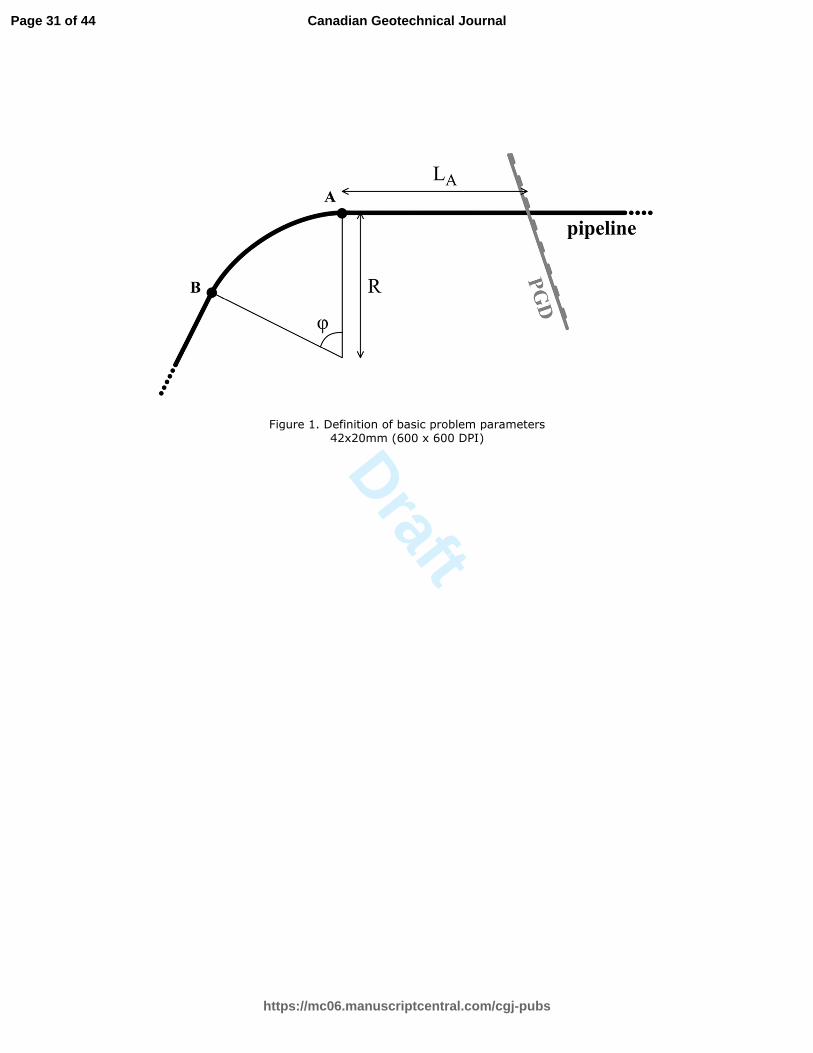
The basic geometrical characteristics of the problem analyzed herein are illustrated in Figure 1. Namely,

a curved pipeline bend of angle φ with a radius of curvature R is located at a distance LA from the point of

PGD application on the pipeline axis. It is assumed that the bend lies outside the high-curvature zone

which develops around the point of PGD application, but inside the pipeline’s unanchored length, so that

Page 4 of 44



Draft

5

it will affect the overall pipeline behavior. Simplified criteria to check LA against the limiting distances

resulting from the above requirements will be presented in following paragraphs.

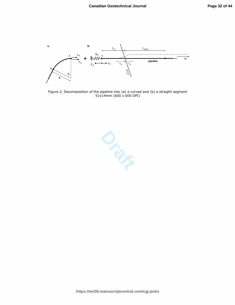
The proposed methodology is based on the decomposition of the pipeline into a straight and a curved

segment, based on endpoint A of the bend towards the PGD zone, as shown in Figure 2. Following this

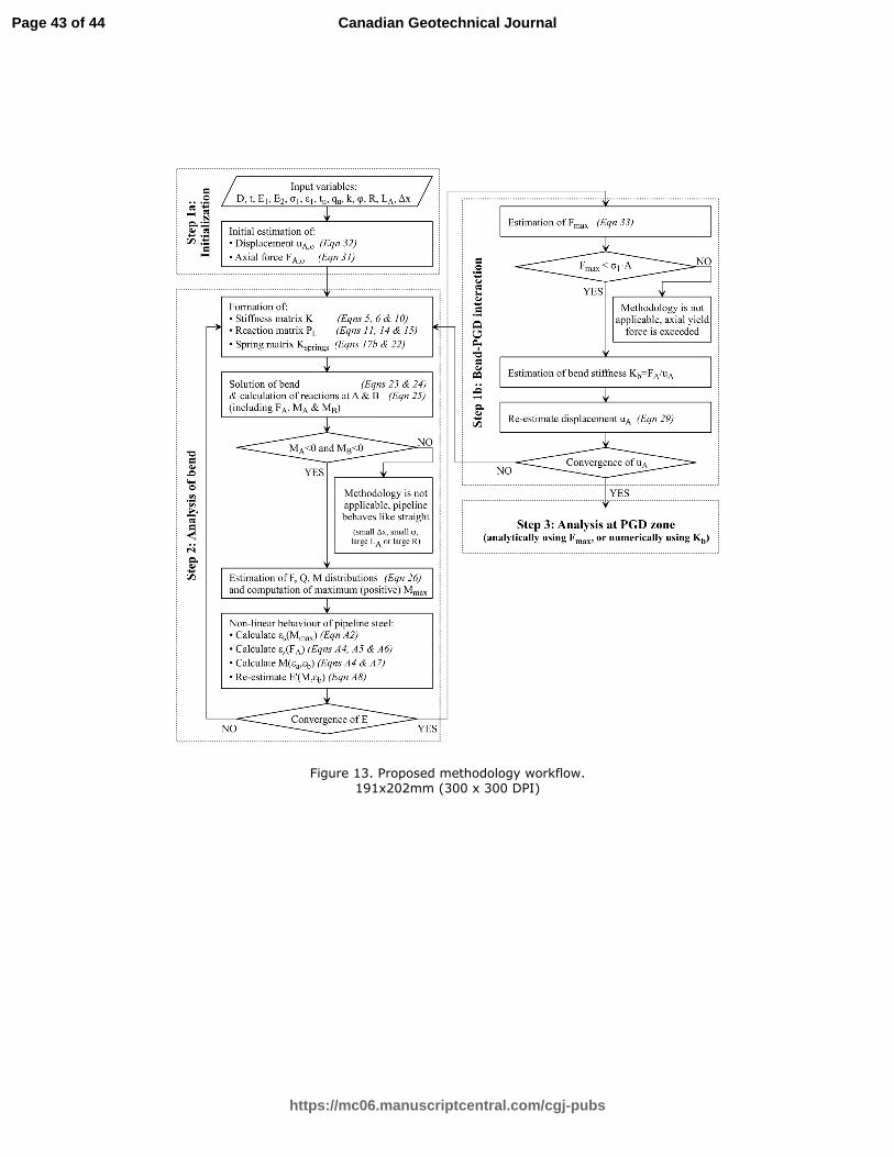
decomposition, analytical computations may be grouped in the following three basic sequential steps:

a. The 1st step focuses on the interaction between the bend and the applied PGD. More specifically, the

axial displacement uA of endpoint A of the bend is calculated as a function of the axial component ∆x

of the applied PGD, by imposing displacement compatibility along the straight segment of the pipeline

shown in Figure 2b.

b. In the 2nd step, this displacement is applied to the curved part of the pipeline shown in Figure 2a and

the resulting internal loads are calculated with the direct stiffness method, assuming that the bend

behaves as an elastic arched beam. During this step, an equivalent secant Young’s modulus is utilized

for the pipeline steel and the analysis is performed iteratively, in order to take into account the

associated non-linear response.

c. In the 3rd step, the axial force FA and the displacement uA at point A, computed from previous steps 1

and 2, are utilized to calculate the maximum axial force Fmax developing in the point of PGD

application. This is consequently implemented into existing analytical methodologies for straight

pipeline segments to calculate the strains associated with the PGD zone. Alternatively, the bend can be

replaced by an axial spring with stiffness Kb=FA/uA and a numerical analysis can be performed, only

focusing on the remaining straight segment and hence reducing the associated computational effort.

Taking into account that the axial displacement uA derived from the 1st step depends also on the stiffness

Kb of the bend which is computed in the 2nd step, it is realized that the 1st and 2nd steps above must be

repeated until convergence is accomplished. In order to clarify this iterative procedure, a methodology

workflow in presented in Appendix 2.

Page 5 of 44



Draft

6

It should be emphasized that the present study refers exclusively to PGDs resulting in pipeline elongation,

with tension being the prevailing mode of pipeline deformation. In cases where the applied PGD imposes

compression to the pipeline (e.g. reverse faults), global pipeline buckling is possible and consequently the

resulting strains should be estimated with detailed numerical analyses. Further than that, it is noted that

the applied PGD may or may not follow a step-like deformation mode, as the detailed PGD distribution

affects primarily the pipeline response in the adjacent high-curvature zone, while the response of the bend

depends mostly on the component of the total displacement applied along the pipeline axis. Nevertheless,

the assumption of step-like deformations, apart from being conservative for the overall pipeline

verification, allows the proposed methodology to be directly combined with existing analytical solutions

for the estimation of pipeline strains at the PGD zone, thus avoiding the use of additional more involved

case-specific numerical analyses.

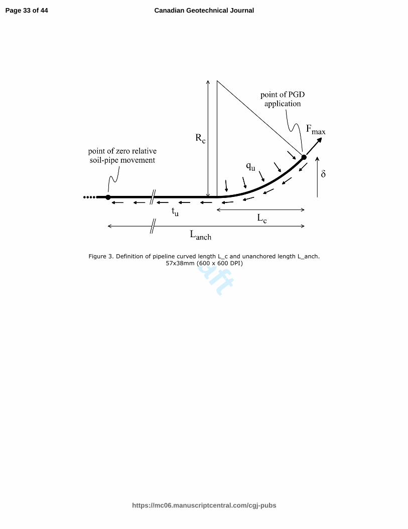
Limits of bend distance from the PGD zone

As mentioned earlier, the proposed methodology applies when the distance LA of the bend from the PGD

zone is (a) larger than the “pipeline curved length” Lc, i.e. the intensely curved length of the pipeline

adjacent to the point of PGD application, and (b) smaller than the "pipeline unanchored length" Lanch, i.e.

the distance from the point of PGD application to the point where relative pipeline-soil displacement

becomes zero. This is because, for distances shorter than Lc, the simplifying assumptions of the

methodology are not valid, while, for distances larger than Lanch, the presence of the bend becomes

indifferent for pipeline verification. It is fortunate that the above distance limits can be readily estimated

in terms of known in advance input parameters (i.e. the applied PGD, the pipeline characteristics and the

ultimate soil reactions), before proceeding with the analytical computations.

More specifically, for large applied displacements, where the whole pipeline cross-section has undergone

yielding, the “curved length” Lc on each side of the applied PGD may be geometrically approximated as

(Kennedy et al. 1977):

Page 6 of 44



Draft

7

c cL 2R= δ (1)

where Rc is the radius of curvature of the pipeline, estimated as:

maxc

u

FR

q= (2)

In the above equations, Fmax is the maximum axial force developing at the point of PGD application, qu is

the ultimate transverse soil resistance and δ is the component of the applied PGD perpendicular to the

pipeline axis (Figure 3).

Taking into account that the methodology of Kennedy et al (1975) assumes complete yielding of the

pipeline cross-section, Fmax may be preliminarily estimated as the cross-sectional area of the pipe times

the tensile yield strength of the pipeline steel. The remaining two parameters (δ and qu) are defined in

relation to the direction of the PGD. Namely, in the case of a lateral horizontal ground displacement ∆h

(e.g. at strike-slip fault crossings), the pipeline deforms symmetrically on both sides of the point of PGD

application, so that δ=∆h/2, while qu corresponds to the ultimate soil resistance for lateral pipeline

movement. In the case of vertical displacement ∆v (e.g. normal faults), pipeline deformations are

asymmetric, as the soil resistance to pipeline uplifting is significantly smaller than that for downward

pipeline movement. Therefore, most of the applied vertical displacement is accommodated through

pipeline uplifting over the hanging wall of the ground rupture, so that δ≈∆v, while qu corresponds to the

uplift resistance of the backfill soil. In either case, parametric application of the above equations indicates

that for typical buried pipelines and applied PGDs, the curved length does not exceed a few tens of

pipeline diameters.

In order to ensure that there is no interaction between the bend and the PGD zone, the minimum distance

LA should also include an additional attenuation length Latt, large enough to accommodate any significant

pipeline deformations developing beyond the curved length Lc, as well as beyond the bend (i.e. to the

Page 7 of 44



Draft

8

right of point A, in Figure 1). In other words, the minimum distance between the bend and the PGD zone

should be larger than LA>Lc+Latt. This attenuation length can be estimated by considering the equivalent

problem of a laterally loaded single pile in elastic homogenous soil. Based on the analytical expression,

by Karatzia and Mylonakis (2012), for the active length beyond which the behavior of a laterally loaded

pile becomes independent of its length, Kouretzis et al (2014) estimated the attenuation length for the case

of buried pipelines as Ltol≈10D, with D being the pipeline’s diameter.

In general, ground displacements will impose a component ∆x parallel to the pipeline axis, resulting in

the development of tension or compression along the pipeline length. In the case of tension examined

herein, the applied elongation ∆x is accommodated through tensile strains along the “pipeline unanchored

length” Lanch (Figure 3). For small and moderate applied elongations, where the axial force on the pipeline

does not exceed the corresponding yield strength, the unanchored length on each side of the PDG

application point can be estimated as (Karamitros et al. 2007):

1anch

u

E A xL

t

∆= (3)

where E1 is the elastic Young’s modulus of the pipeline steel, A is the pipeline’s cross-section area and tu

is the ultimate friction between the pipeline and the surrounding soil. Parametric application of the above

equation for typical buried pipelines indicates that the unanchored length is significantly larger than the

corresponding curved length and may extend to several hundreds of pipeline diameters on each side of the

ground rupture.

Analysis of the bend

The core of the proposed methodology is the structural analysis of the bend (i.e. the 2nd step referenced in

Basic assumptions), hence its presentation will precede that of the 1st and the 3rd steps of the methodology

which have to do with the interaction between the bend and the PGD zone. More specifically, the pipeline

Page 8 of 44



Draft

9

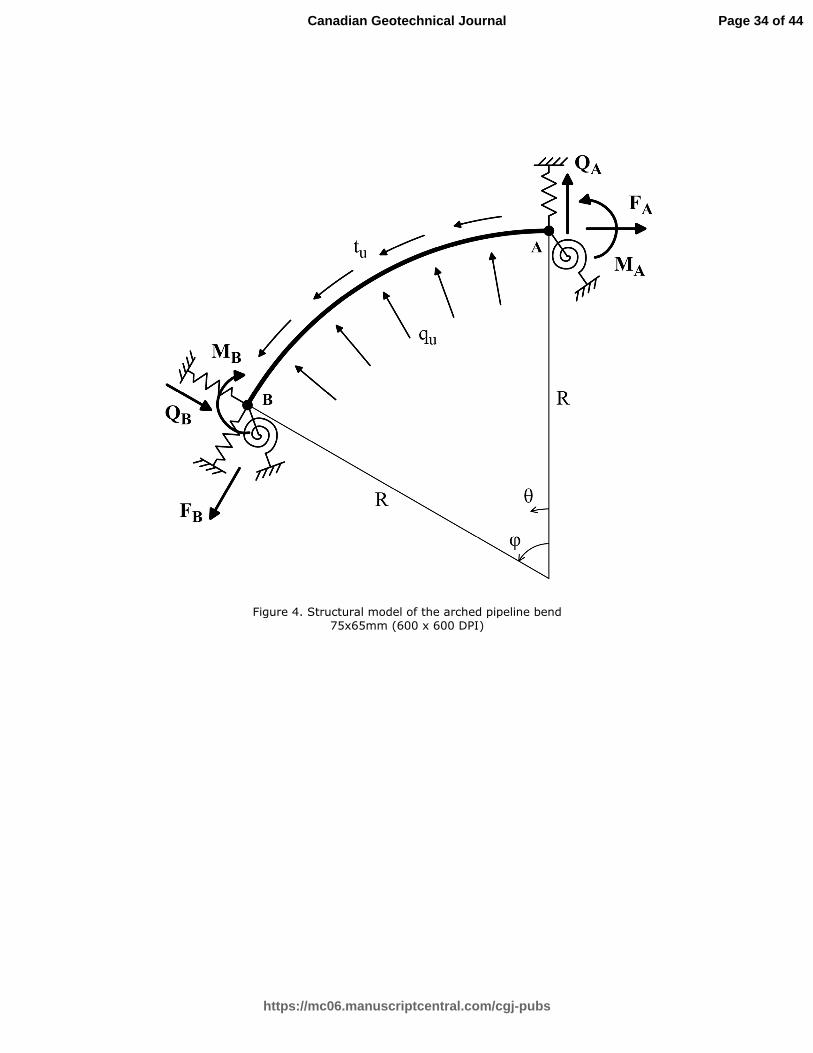
bend is analyzed as an elastic arched beam AB, subjected to an axial displacement uA at the edge towards

the PGD zone, as shown in Figure 4. Apart from uA, the beam is loaded with an axial uniformly

distributed load tu equal to the ultimate friction force applied by the surrounding soil, as well as a

transverse load qu, equal to the ultimate soil resistance for transverse horizontal pipeline displacement.

Furthermore, rotational and transverse transitional springs are considered at both ends of the arch, while

an additional axial spring is considered at end B.

The bend is subsequently solved using the direct stiffness method:

{ } { } [ ]( ){ }L sprP P K K u − = + (4)

where {P}={FA QA MA FB QB MB}T are the axial forces F, shear forces Q and bending moments M at the

ends Α and Β of the beam, {PL} are the respective reaction forces corresponding to loads tu and qu, [K] is

the (6×6) stiffness matrix of the arched beam, [Kspr] is the (6×6) support springs matrix and {u}={uA vA

φΑ uB vB φB}T are the axial displacements u, the transverse displacements v and the rotations φ of

endpoints Α and Β of the beam. The corresponding matrices are derived as follows.

Stiffness matrix K

Considering the curved beam’s equilibrium, without the external loads tu and qu which are treated

separately, yields:

{ } [ ]{ }B B

B A

A A

B A

cos sin 0

sin cos 0

R(co

F F

P

s 1) R sin 1

Q Q P

M M

ϕ ϕ = − ϕ ϕ ϕ− ϕ

= = Λ

(5)

Therefore, the stiffness matrix [K] can be formed with the aid of the above transpose matrix [Λ]:

Page 9 of 44



Draft

10

[ ][ ] [ ]( ) [ ]

[ ][ ] [ ] [ ]( ) [ ]

T1 1

T1 1

F FK

F F

− − Τ

− − Τ

Λ =

Λ Λ Λ

(6)

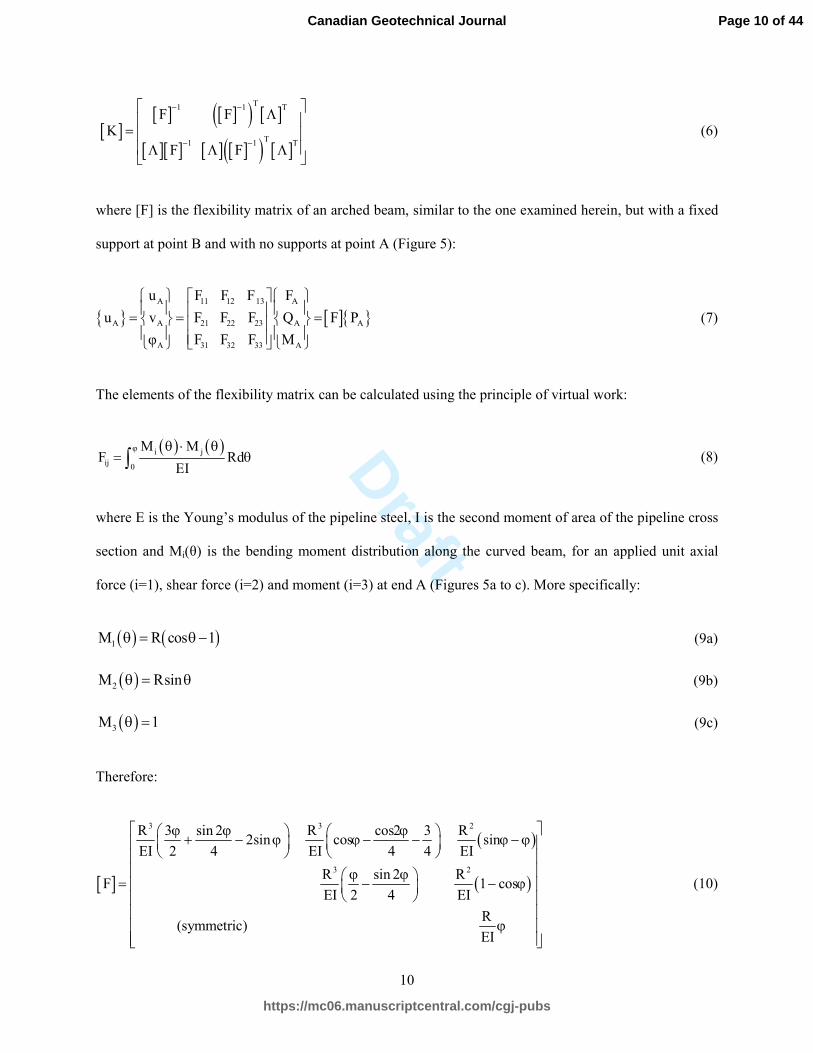
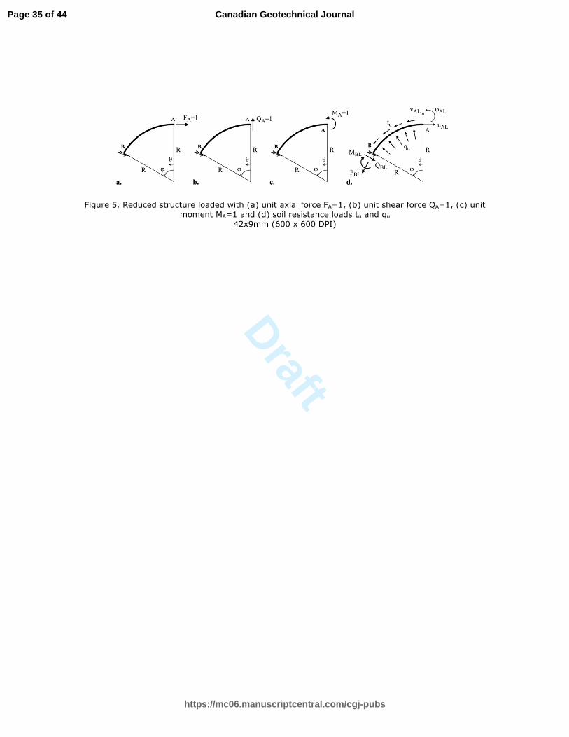
where [F] is the flexibility matrix of an arched beam, similar to the one examined herein, but with a fixed

support at point B and with no supports at point A (Figure 5):

{ } [ ]{ }A 11 12 13 A

21 22 23

31 32 33

A A A A

A A

F F F

F F F

F F

u F

u v Q F P

φ F M

=

= =

(7)

The elements of the flexibility matrix can be calculated using the principle of virtual work:

( ) ( )i j

ij 0

M MF Rd

EI

ϕ θ ⋅ θ= θ∫ (8)

where E is the Young’s modulus of the pipeline steel, I is the second moment of area of the pipeline cross

section and Mi(θ) is the bending moment distribution along the curved beam, for an applied unit axial

force (i=1), shear force (i=2) and moment (i=3) at end A (Figures 5a to c). More specifically:

( ) ( )1M R cos 1=θ θ− (9a)

( )2M Rsin=θ θ (9b)

( )3M 1θ = (9c)

Therefore:

[ ]

( )

( )

3 3 2

3 2

R 3 sin 2 R cos 3 R2sin cos sin

EI 2 4 EI 4 4 EI

R sin 2 R1 cos

EI

2

F

(symme

2 4 EI

Rt )

EIric

ϕ ϕ + − ϕ − − ϕ −ϕ ϕ

ϕ ϕ

=

ϕ − − ϕ

ϕ

(10)

Page 10 of 44



Draft

11

Reaction force matrix PL

Considering the same arched cantilever beam with a fixed support at point B (Figure 5d), the reactions to

the applied soil friction forces tu and the transverse soil resistance forces qu may be calculated using

equations of equilibrium:

{ }( )

( )( ) ( )

BL u u

BL u u

2

BL

2BL u u

F R 1 cos R t sin

Q R sin Rt 1 cos

M R q 1 cos R t sin

q

P q

= = ϕ +

− ϕ − ϕ

− ϕ

− ϕ + ϕ− ϕ

(11)

The bending moment distribution due to the applied soil reaction forces may be derived by substituting φ

with θ, in the above equation:

( ) ( )2 2L u uM R t sin R q 1 cos= θθ− + − θ (12)

Hence, using Equations 9 and 12, the corresponding axial displacement (i=1), transverse displacement

(i=2) and rotation (i=3) of point Α may be calculated, based on the principle of virtual work, as:

( ) ( )i LAL,i 0

M MRd

EI

ϕ θ ⋅ θ∆ = θ∫ (13)

Finally:

{ }

( )

2

u u

AL 3 2

AL u u

AL2

u

2

u

AL

sin sin 3t sin q 2sin

2 4 2u

R sin sinv t sin cos q 1 cos

EI 2 4 2

t cos 1 +q

2R R

2

2R R

si2

n

ϕ ϕ + ϕ −

ϕ ϕ = ⋅ − − + + − −

ϕ ϕϕ ϕ− − −

ϕ∆

ϕ ϕ + ϕ −

= ϕ ϕ ϕ ϕ

ϕ− ϕ

(14)

Utilizing the above matrix, in combination with [F] and [Λ], the reaction matrix {PL} may be formed:

Page 11 of 44



Draft

12

{ }[ ] { }

{ } [ ][ ] { }

1

AL

L 1

BL AL

FP

P F

−

−

− ∆ =

− Λ ∆ (15)

Note that in the Direct Stiffness Method, the opposite of this matrix (i.e. -{PL}) is applied to the beam as a

loading, as indicated by Equation 4.

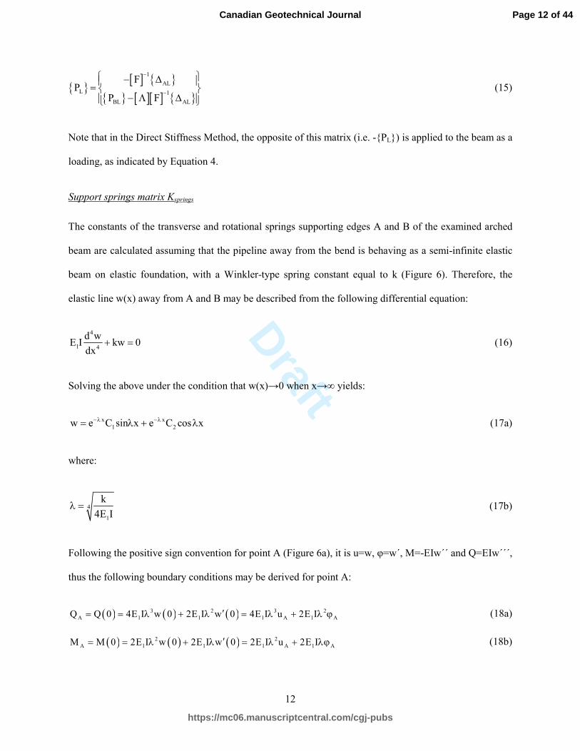
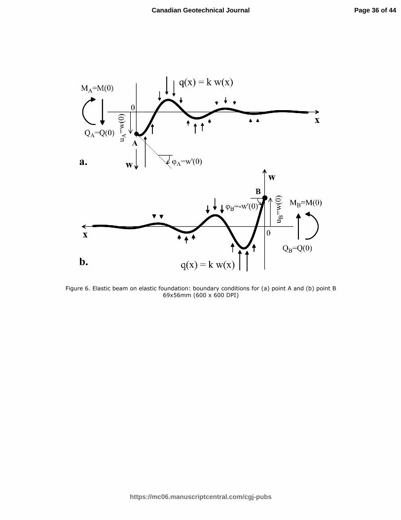
Support springs matrix Ksprings

The constants of the transverse and rotational springs supporting edges A and B of the examined arched

beam are calculated assuming that the pipeline away from the bend is behaving as a semi-infinite elastic

beam on elastic foundation, with a Winkler-type spring constant equal to k (Figure 6). Therefore, the

elastic line w(x) away from A and B may be described from the following differential equation:

4

1 4

d wkw 0

dxΕ Ι + = (16)

Solving the above under the condition that w(x)→0 when x→∞ yields:

x x1 2xw e C sin e C c s xo−λ −λ= +λ λ (17a)

where:

4

1

k

4E Iλ = (17b)

Following the positive sign convention for point A (Figure 6a), it is u=w, φ=w΄, M=-EIw΄΄ and Q=EIw΄΄΄,

thus the following boundary conditions may be derived for point A:

( ) ( ) ( )3 2 3 2A 1 1 1 A 1 AQ Q 0 4E I w 0 2E I w 0 4E I u 2E I′= = λ + λ = λ + λ ϕ (18a)

( ) ( ) ( )2 2A 1 1 1 A 1 AM M 0 2E I w 0 2E I w 0 2E I u 2E I′= = λ + λ = λ + λϕ (18b)

Page 12 of 44



Draft

13

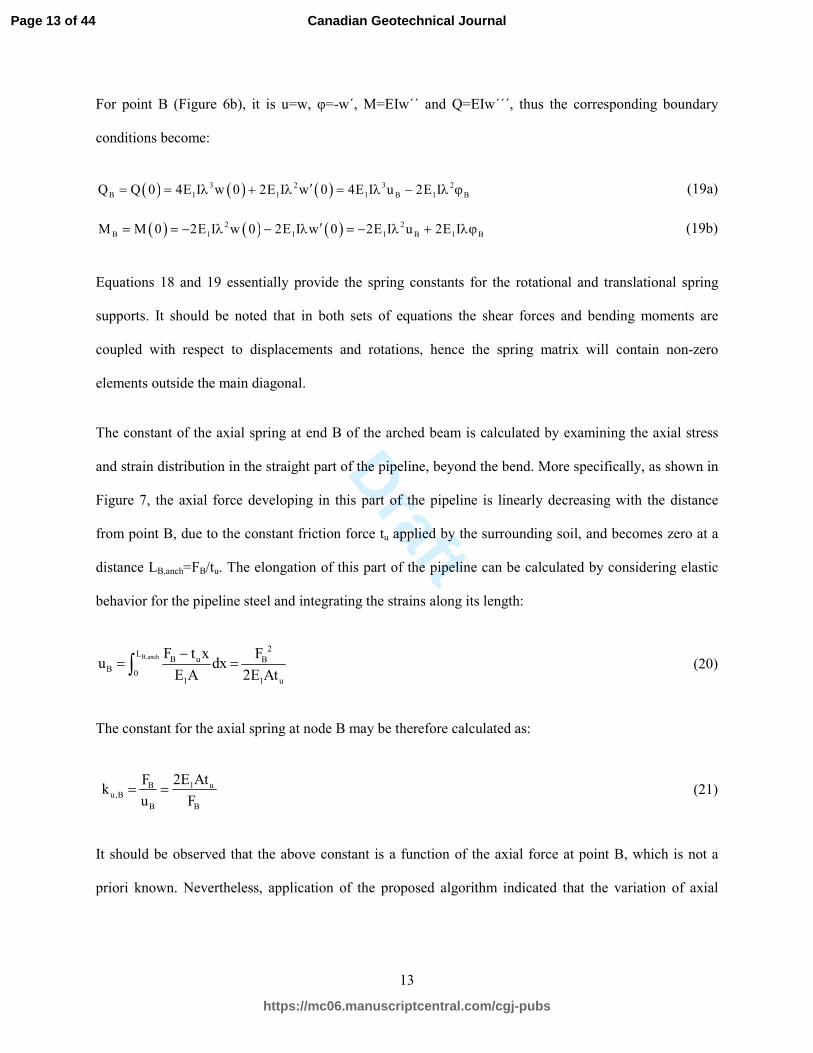
For point B (Figure 6b), it is u=w, φ=-w΄, M=EIw΄΄ and Q=EIw΄΄΄, thus the corresponding boundary

conditions become:

( ) ( ) ( )3 2 3 2B 1 1 1 B 1 BQ Q 0 4E I w 0 2E I w 0 4E I u 2E I′= = λ + λ = λ − λ ϕ (19a)

( ) ( ) ( )2 2B 1 1 1 B 1 BM M 0 2E I w 0 2E I w 0 2E I u 2E I′= = − λ − λ = − λ + λϕ (19b)

Equations 18 and 19 essentially provide the spring constants for the rotational and translational spring

supports. It should be noted that in both sets of equations the shear forces and bending moments are

coupled with respect to displacements and rotations, hence the spring matrix will contain non-zero

elements outside the main diagonal.

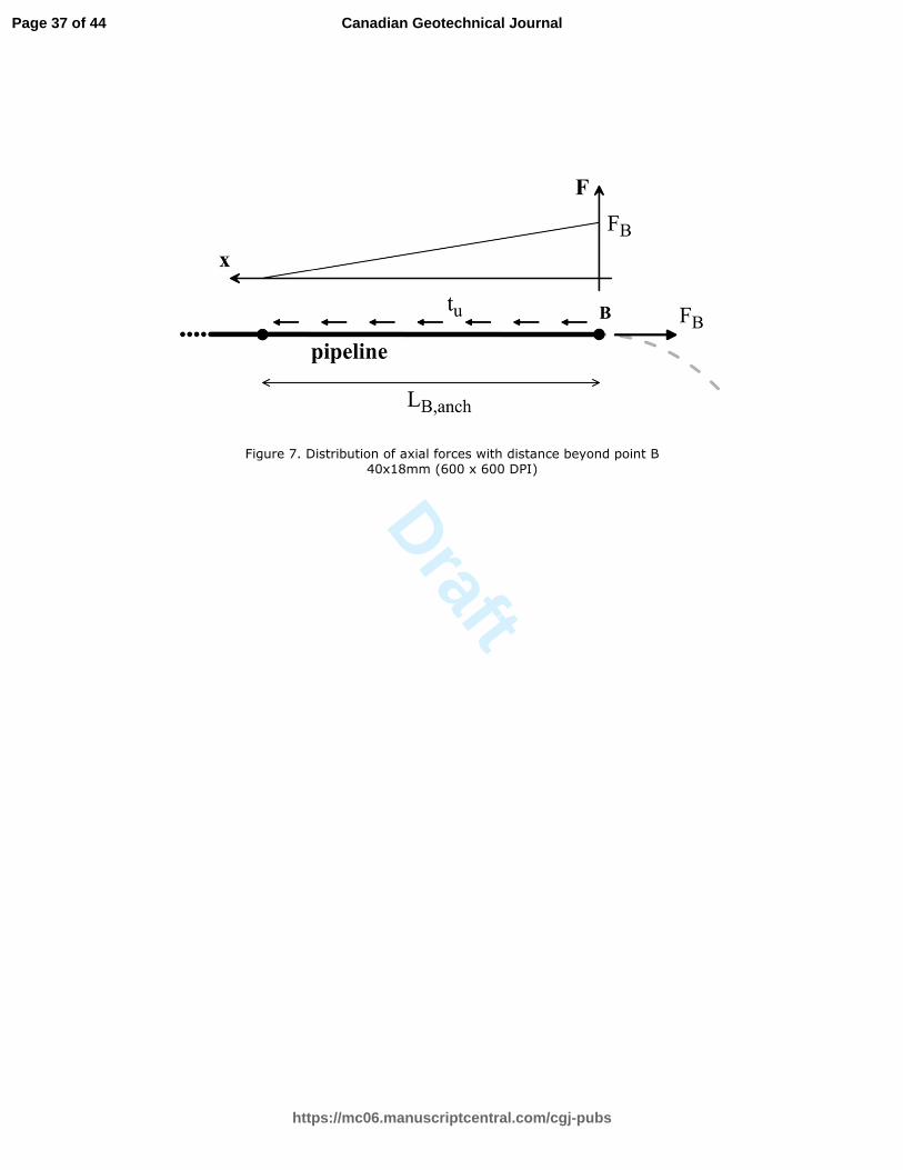
The constant of the axial spring at end B of the arched beam is calculated by examining the axial stress

and strain distribution in the straight part of the pipeline, beyond the bend. More specifically, as shown in

Figure 7, the axial force developing in this part of the pipeline is linearly decreasing with the distance

from point B, due to the constant friction force tu applied by the surrounding soil, and becomes zero at a

distance LB,anch=FB/tu. The elongation of this part of the pipeline can be calculated by considering elastic

behavior for the pipeline steel and integrating the strains along its length:

B,anch2

LB u B

01 1 u

F t x Fu dx

E A 2E AtΒ

−= =∫ (20)

The constant for the axial spring at node B may be therefore calculated as:

1 uu,B

B

2E AtFk

u FΒ

Β

= = (21)

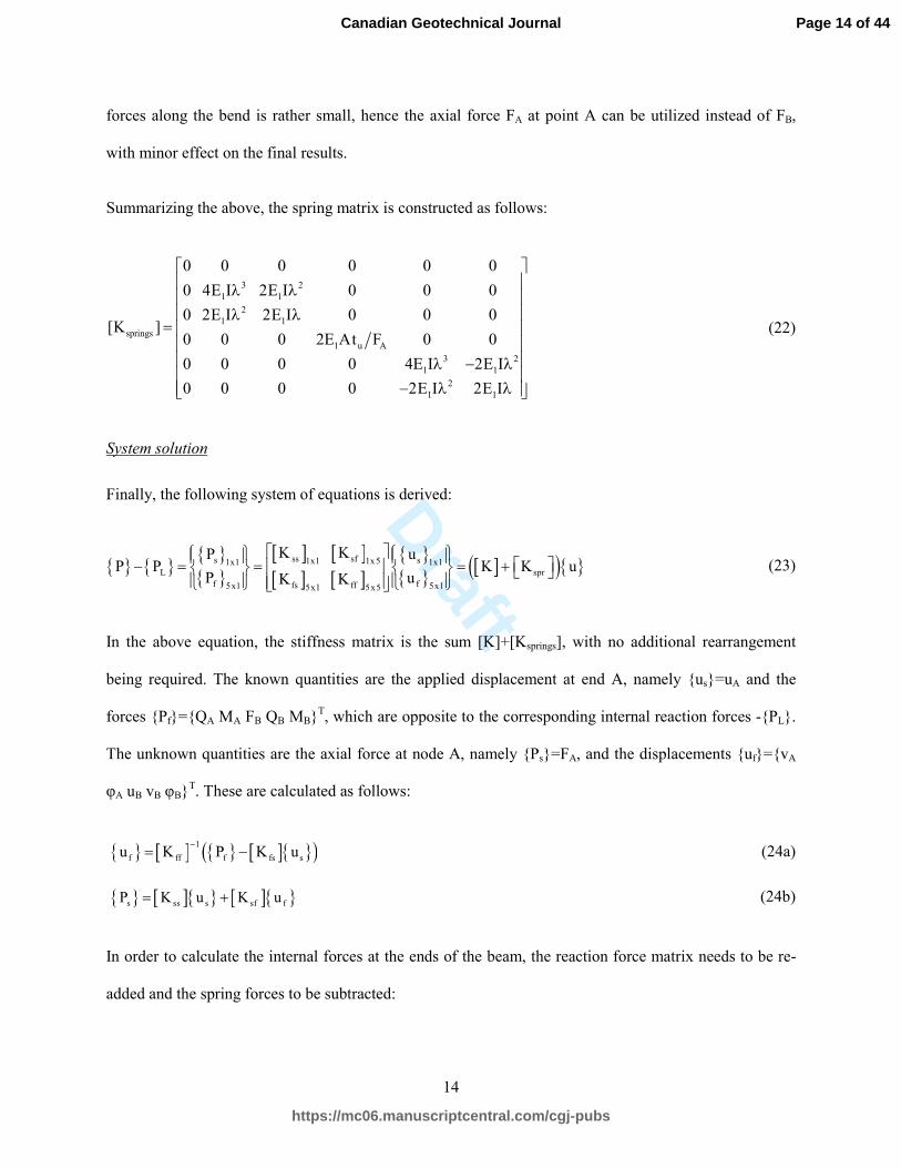
It should be observed that the above constant is a function of the axial force at point B, which is not a

priori known. Nevertheless, application of the proposed algorithm indicated that the variation of axial

Page 13 of 44



Draft

14

forces along the bend is rather small, hence the axial force FA at point A can be utilized instead of FB,

with minor effect on the final results.

Summarizing the above, the spring matrix is constructed as follows:

3 21 1

21 1

springs1 u

3 21 1

A

21 1

F

0 0 0 0 0 0

0 4E I 2E I 0 0 0

0 2E I 2E I 0 0 0[K ]

0 0 0 2E At 0 0

0 0 0 0 4E I 2E I

0 0 0 0 2E I 2E I

λ λ λ λ

= λ − λ

− λ λ

(22)

System solution

Finally, the following system of equations is derived:

{ } { }{ }{ }

[ ] [ ][ ] [ ]

{ }{ } [ ]( ){ }ss sfs s1x1 1x51x1 1x1

L sprf ffs ff5x1 5x15x1 5x5

KP uP P K K u

P uK K

Κ − = = = +

(23)

In the above equation, the stiffness matrix is the sum [K]+[Ksprings], with no additional rearrangement

being required. The known quantities are the applied displacement at end A, namely {us}=uA and the

forces {Pf}={QA MA FB QB MB}T, which are opposite to the corresponding internal reaction forces -{PL}.

The unknown quantities are the axial force at node A, namely {Ps}=FA, and the displacements {uf}={vA

φΑ uB vB φB}T. These are calculated as follows:

{ } [ ] { } [ ]{ }( )1

f ff f fs su K P K u−

= − (24a)

{ } [ ]{ } [ ]{ }s ss s sf fP K u K u= + (24b)

In order to calculate the internal forces at the ends of the beam, the reaction force matrix needs to be re-

added and the spring forces to be subtracted:

Page 14 of 44



Draft

15

{ } { }{ }

{ } { }{ }

s sL springs

f f

P uP P K

P u

= + − (25)

The distribution of axial forces F(θ), shear forces Q(θ) and bending moments M(θ) can be consequently

derived as:

( ) ( )Α Α u uF F cos Q sin R q 1 cos R t sinθ = θ + θ + − θ − θ (26a)

( ) ( )Α Α u usin cosQ F Q R q sin R t 1 cosθ = − θ + θ + −ϕ + ϕ (26b)

( ) ( ) ( ) ( )2 2Α Α Α u uM F cos 1 +Q Rsin M R q 1 cos R t s nR iθ = θ − θ + + − θ + θ − θ (26c)

Non-linear behavior of pipeline steel

In the previously presented solution, the pipeline was considered to behave elastically. To account for the

non-linear behavior of the pipeline steel, the above procedure is applied iteratively, using an equivalent

secant Young’s modulus E΄ for the pipeline steel, until compatibility is achieved between the stresses and

strains developing on the pipeline, at the position of maximum bending moment Mmax. It is noted that the

negative bending moments calculated for endpoints A and B of the bend may exceed in absolute value the

maximum positive bending moment developing in the middle of the bend. Nevertheless, this is attributed

to the stiffness of the support springs, which have been calculated under the conservative assumption that

the Winkler-type soil springs away from the bend behave elastically. In reality, for large displacements

and rotations of points A and B, the ultimate transverse soil resistance will be reached even beyond the

ends of the bend. This will result in an increase of the overall flexibility of the bend and a reduction of the

developing axial forces and bending moments along the pipeline. In order to remain conservative, the

proposed methodology maintains the assumption of elastic support springs for the bend. However, it is

recommended that the bending moments at endpoints A and B are not taken into account and Mmax is

taken as the maximum positive bending moment.

Page 15 of 44



Draft

16

The procedure adopted for the calculation of E΄ is the same as that initially proposed by Karamitros et al

(2007, 2011), and subsequently adopted by Trifonov and Cherniy (2010, 2012). The basic equations of

the corresponding algorithm are repeated herein as Appendix 1, in order to enable independent reading of

the paper.

Interaction between PGD zone and pipeline bend

Displacement Compatibility

The first element of the interaction between the PGD zone and the pipeline bend is related to the

computation of the axial displacement uA applied at endpoint A of the bend (i.e. the 1st step referred to in

Basic assumptions). This is achieved by considering compatibility of displacements between the axial

component ∆x of the applied PGD, the displacement uA at the beginning of the bend, as well as the

elongation ∆L of the straight segment of the pipeline:

Ax L u∆ = ∆ + (27)

The elongation ∆L is calculated by integrating the axial strains developing along the straight part of the

pipeline. The corresponding strain distribution is determined by assuming an elastic stress-strain behavior

for the pipeline steel, as well as a linear distribution of axial forces along the pipeline’s length, due to a

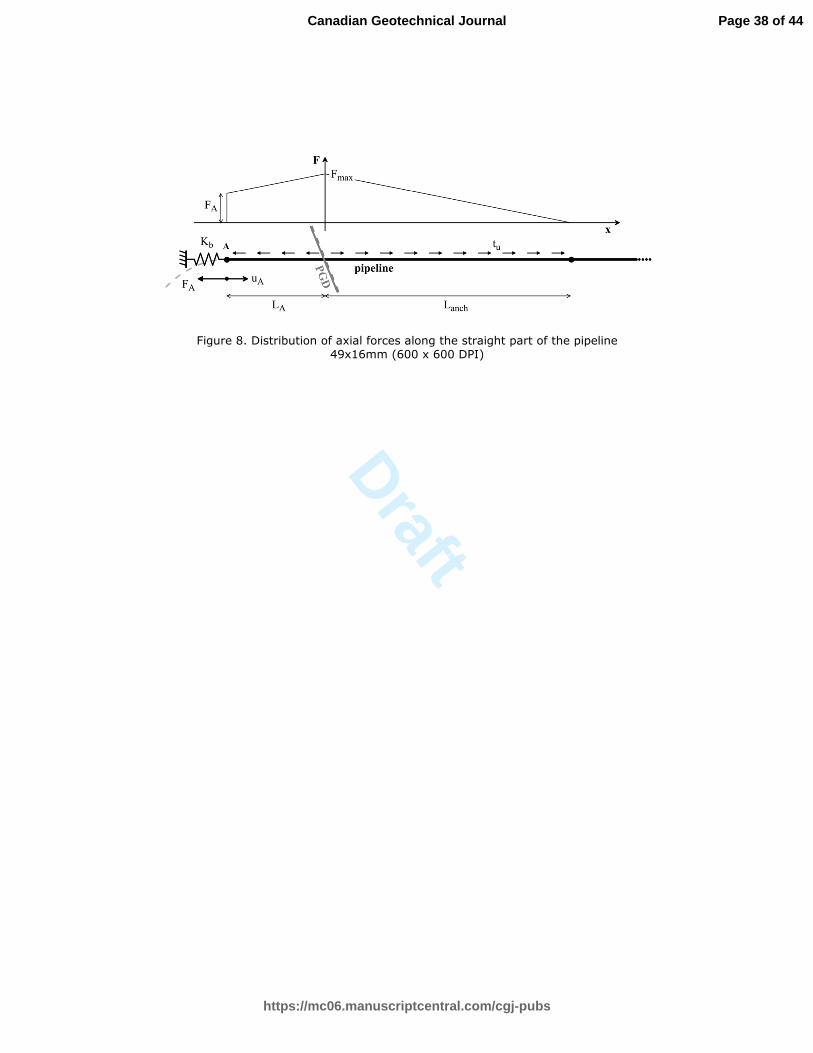
fully mobilized friction force tu applied by the surrounding soil. More specifically, as shown in Figure 8,

the axial force increases from FA at endpoint A of the bend, to Fmax=FA+tuLA at the PGD point of

application, and subsequently decreases to F=0 at a distance Lanch=Fmax/tu. According to the above:

A anch2

L L2u max u A

A A u A0 01 1 1 u

F t x F t x F1L dx dx 2L F t L

E A 2tΑ + −

∆ = + = + + Ε Α Ε Α

∫ ∫ (28)

Page 16 of 44



Draft

17

The axial force FA applied to the end of the bend may be correlated to the corresponding displacement uA

through a stiffness coefficient Kb, as FA=KbuA. In this case, Equations 27 and 28 yield:

( ) ( )2 2 2 21 u A b u 1 u A b u 1 A b u 1 b u

A 2b

E At 2L K t E At 2 L K t 4E AL K t 2E AK t xu

K

− − + + + + ∆= (29)

The stiffness Kb in Equation 29 is not known before analyzing the bend. Therefore, an initial

displacement uA,o is applied to the end of the bend and the reaction FA is consequently determined. Kb is

redefined as FA/uA and the procedure is repeated until convergence (in terms of either Kb, uA or FA) is

achieved.

The displacement uA,o used in the first iteration can be defined as the displacement of the same point A

(i.e. at a distance LA from the PGD location), while assuming that no bend exists in the pipeline route. In

that case, the displacement compatibility equation would become:

anch2

Lmax u max

01 1 u

F t x Fx 2 dx

t

−∆ = ⋅ =

Ε Α Ε Α∫ (30)

Therefore, the axial force FA,o at a distance LA would be equal to:

A,o max u A 1 u u AF F t L t x t L= − = Ε Α ∆ − (31)

and the corresponding displacement would be equal to the integral of axial strains further away from this

point, as:

A ,o u

2F t A,o u A,o

A,o 01 1 u

F t x Fu dx

2 t

−= =

Ε Α Ε Α∫ (32)

It is acknowledged that the above derivation is only valid when the axial strains along the straight

segment of the pipeline remain elastic. Therefore, the proposed methodology is applicable only when:

Page 17 of 44



Draft

18

max A u A 1F F t L A= + < σ (33)

where σ1 is the yield stress of the pipeline steel.

Pipeline verification at the PGD zone

The second element of the interaction between the PGD zone and the pipeline bend is related to the

computation of the pipeline stresses and strains in the vicinity of the application point of the PGD (i.e. the

3rd step referred to in Basic assumptions). More specifically, following the convergence of Steps 1 and 2

of the proposed methodology, the displacement uA and axial force FA at the beginning of the bend are

determined and can be consequently employed for the analysis of the pipeline at the PGD zone.

Depending on the required level of accuracy, there are two ways to accomplish that, as described below:

a. Many of the currently available analytical methodologies for the strength verification of buried

pipelines against step-like PGDs (e.g. Karamitros et al. 2007, 2012 and Trivonov and Cherniy 2011,

2012, for fault crossings, or Kouretzis et al. 2014, for differential settlement or heave) provide

estimations of the corresponding design strains as a function of the maximum axial force Fmax

developing at the point of PGD application. In these methodologies, Fmax is calculated assuming a

straight pipeline route. Nevertheless, having calculated the axial force FA at endpoint A of the bend,

the axial force Fmax can be readily estimated as FA+tuLA and subsequently incorporated into the same

methodologies, in order to quantify the effect of the bend on the pipeline behavior at the PGD zone.

b. If the strains developing near the PGD zone are critical for pipeline design, a more detailed numerical

analysis may be required. An accurate simulation of the pipeline bend in this case might result in

complicated meshes that require a lot of time and expertise to be created. Nevertheless, this can be

avoided by replacing the bend with an elastic axial spring, featuring a stiffness of Kb=FA/uA. This

would introduce the effect of the bend on pipeline performance, while significantly reducing the

overall computational effort.

Page 18 of 44



Draft

19

Evaluation of proposed methodology

The accuracy of the proposed methodology was evaluated through comparison with numerical predictions

from parametric analyses with the Finite Element Method and the commercial code ANSYS 12 (ANSYS

Inc. 2009). A typical high-pressure natural gas pipeline was considered for this purpose, featuring an

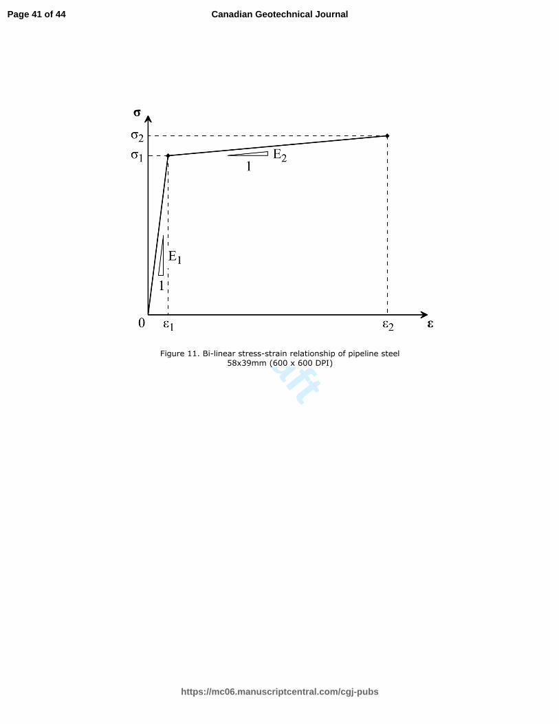
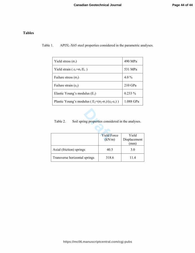
external diameter of D=0.9144m (36'') and a wall thickness of t=0.0119m. The pipe was made of API5L-

X65 carbon steel, the behavior of which was described by a bi-linear stress-strain relationship, with the

properties listed in Table 1. The pipeline route included a bend of angle φ, which varied parametrically

from 0° (straight axis) to 90°, with a radius of curvature R, which similarly varied from 5D to 40D. The

pipeline was discretized in 0.50m long elastoplastic beam elements, for a sufficient length on both sides

of the point of PGD application, so that forces and displacements at the far ends diminish to zero.

To simulate soil-pipeline interaction, each node of the pipeline was connected to axial and transverse

horizontal Winkler springs, modeled as elastic-perfectly plastic rod elements. The spring properties were

calculated according to the ALA-ASCE (2005) guidelines, assuming that the pipeline is buried into silica

sand backfill, with friction angle φ=36º and dry unit weight γ=18ΚΝ/m2. A burial depth of 1.30m was

considered, measured from the top of the pipe, resulting in the spring properties of Table 2. Since the

applied ground displacements were horizontal, no vertical soil springs were utilized in the analyses and

the corresponding degrees of freedom of the pipeline nodes were fixed.

The examined PGD involved a step-like movement of a seismic strike-slip fault, crossing the pipeline

route at an angle of 45° and resulting in pipeline elongation. Fault displacements ∆f of up to 2.0D were

applied to the fixed end of the Winkler springs over the sliding wall of the fault, corresponding to a

maximum axial ∆x displacement of 2D . The distance LA between the fault crossing and the bend was

varied parametrically from 50D to 200D, as compared to the maximum estimated "pipeline curved

length" Lc≈10D and the maximum "pipeline unanchored length" Lanch≈500D.

Page 19 of 44



Draft

20

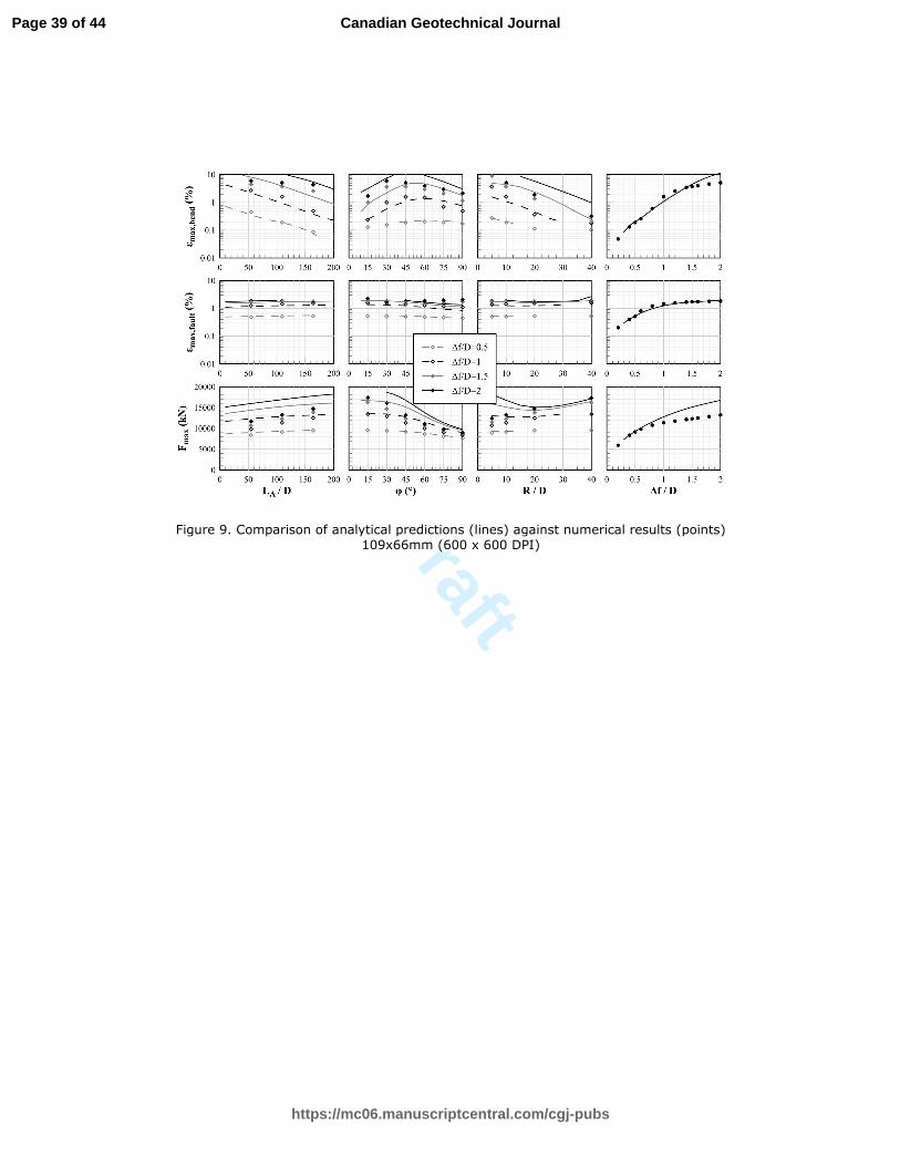
The numerical and the analytical predictions are compared in the graphs of Figure 9, with each column of

graphs focusing separately on the effects of the normalized bend distance LA/D, the bend angle φ and the

radius of curvature R/D, as well as of the normalized applied fault displacement ∆f/D. Note that the

parametric analyses compared in Figure 9 were performed with reference to a basic case with LA/D=100,

φ=45° and R/D=10. The first row of graphs refers to the maximum longitudinal pipeline strains

developing at the bend (εmax,bend), while the following two rows refer to the maximum strains developing

in the vicinity of the fault crossing (εmax,fault) and the maximum axial force developing at the fault trace

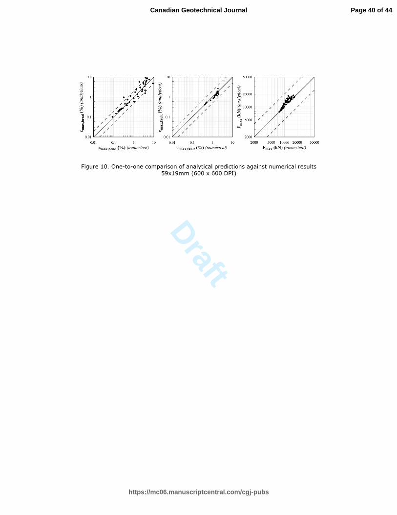
(Fmax). In addition, Figure 10 shows one-to-one comparisons for the above pipeline response measures,

for the entire range of the input parameters. Note that the analytical predictions of εmax,fault in the above

figures were obtained by combining the methodology proposed herein with the analytical solution of

Karamitros et al (2007), for straight pipelines segments crossing strike-slip faults.

Examination of the maximum bend strains εmax,bend, in the first row of graphs of Figure 9 reveals that they

may become significant and may even surpass the corresponding strains at the PGD zone by an order of

magnitude as the distance of the bend from the displacement zone decreases and the curvature

characteristics of the bend become more intense, i.e. the bend angle φ increases and the radius of

curvature R decreases. Furthermore, it is worth to observe that the most severe condition corresponds to

intermediate bend angles φ=30-45ο and not to right bend angles φ=90ο, as it could be conventionally

thought.

Focusing next on the pipeline strains and forces at the vicinity of the PGD zone, in the 2nd and 3rd rows of

graphs in Figure 10, it is observed that there is a relatively minor effect from the presence of the bend

which could be approximately overlooked. It is also interesting that the contribution of the bend was

actually beneficial for bend angles φ>45ο, as the existence of the bend added flexibility to the system,

resulting in reduced axial forces at the fault crossing. This is because a large part of the axial component

of the applied displacement was undertaken by pipeline bending (at the curved part of the bend), instead

of pipeline tension (at the straight part before the bend), as the bending stiffness EI of hollow cross-

Page 20 of 44



Draft

21

sections is considerably smaller than the corresponding axial stiffness EA. However, taking into account

that the overall stiffness also depends on soil reactions, it is speculated that this trend may be reversed for

large transverse soil resistances (e.g. stiffer soil and/or larger burial depths) and small soil-pipe friction

coefficients (e.g. when a pipeline liner is installed).

The analytical predictions capture the above trends with notable accuracy. In quantitative terms, for small

and medium applied displacements, where the developing strains do not exceed 0.5%, the deviation

between the analytically calculated maximum bend strains εmax,bend and the corresponding numerical

results remains below 20%. Consistency is maintained for larger displacements, however the scatter

gradually increases. This is attributed to the fact that large strains are associated with the formation of a

plastic hinge within the bend, which cannot be accurately captured using an equivalent-linear

approximation. A similar trend is observed for the maximum strains εmax,fault developing in the vicinity of

the fault crossing. The methodology of Karamitros et al (2007) provides accurate estimations for small

and medium strain levels of up to 0.5%. For larger deformations, where the pipeline behavior becomes

highly non-linear, the corresponding strains are under-predicted by an average of 15%. Regarding the

maximum axial force Fmax developing at the fault trace, the proposed methodology consistently provides

conservative estimations. This is due to the assumption of elastic support springs for endpoints A and B

of the bend, which increase the overall stiffness of the system.

Finally, it is noted that some of the analytical predictions are omitted from Figures 9 and 10. For large

normalized fault displacements ∆f, large fault-bend distances LΑ/D and small bending angles φ, this is

because the analytically predicted Fmax exceeded the yield strength of the pipeline, hence the assumption

that the straight segment of the pipeline behaves elastically was no longer valid. In the case of smaller

fault displacements ∆f/D, small bending angles φ and large radii of curvature R/D, the bending moments

developing at the bend became positive at endpoints A and B and negative in the middle, contrary to what

was expected. This is attributed to the fact that the proposed methodology assumes mobilization of the

ultimate transverse soil resistance along the arc AB, which is not realistic when the pipeline is almost

Page 21 of 44



Draft

22

straight. Therefore, the proposed methodology should only be employed under the requirement that the

computed MA and MB remain negative.

Concluding remarks

A simplified analytical methodology has been proposed, facilitating the stress analysis of buried pipelines

against permanent ground displacements (PGDs), in the existence of a bend along the pipeline route. The

methodology is applicable for PGDs resulting in pipeline elongation, with the bend being located within

the pipeline unanchored length, yet outside the high-curvature zone adjacent to the application point of

the PGD. It is acknowledged that during the presentation and verification of the proposed methodology,

the flexibility of the bent part of the pipeline has been considered equal to that of a straight pipe. Even

though this assumption is typical in many practical engineering applications, it should be clarified that the

bending stiffness of curved thin-walled pipes can be significantly decreased due to the von Karman effect

(e.g. Öry and Wilczek 1983). However, this effect is diminished due to the pipeline’s internal pressure

(Bathe and Almeida 1982) and the adjacency with straight segments (Thomas 1981), while it may also be

affected by the interaction with the surrounding soil. Nevertheless, in case that the user wishes to consider

an increased flexibility for the curved part of pipeline, this can be readily performed in the proposed

methodology, through an equivalent adjustment of the corresponding bending stiffness. Furthermore, it is

acknowledged that the proposed methodology does not account for the effects of local buckling and

section deformation and consequently its application should not be extended beyond the strain limits

defined by design codes for such phenomena to be avoided.

Comparison between analytical predictions obtained with the proposed methodology and results from

non-linear numerical analyses with the Finite Element Method indicated a good agreement for a wide

range of the input parameters. Further than that, the parametric numerical and analytical predictions

reviewed in this study revealed a number of practical conclusions with regard to the overall design of

pipelines with bends against PGDs. In summary:

Page 22 of 44



Draft

23

• Under the conditions stated above, the effect of bends on pipeline strains developing at the zone of the

applied PGD is relatively minor and may be approximately overlooked. In the typical case examined

herein, the effect of bend has proved even beneficial for bend angles φ>45ο, as a large part of the axial

component of the applied displacement was undertaken by the bend and not by the straight pipeline

segment in front of it.

• Nevertheless, pipeline strains at the bend may exceed the strains at the PGD zone, and become critical

for the pipeline design. The difference may reach an order of magnitude, for bend angles φ=30-45°

and relatively small radii of curvature R/D<20.

• The assumption of 90o bend angles is not always conservative, as it is commonly considered in

practice.

• Large pipeline strains at bends may be efficiently mitigated by proper design of the pipeline routing.

Namely, bends should be placed at a sufficiently large distance from the PGD zone, bend angles

should be reduced below 30o and radii of curvature should be increased above 15-20D.

References

ANSYS Inc. ANSYS release 12.0 documentation, 2009.

American Lifelines Alliance—ASCE 2005. “Guidelines for the Design of Buried Steel Pipe”, July 2001

(with addenda through February 2005).

Bathe, K.J., and Almeida, C.A. 1982. “Simple and effective pipe elbow element - Pressure stiffening

effects”, Journal of Applied Mechanics, Transactions ASME, 49 (4), pp. 914-916.

Cocchetti, G., di Prisco, C., and Galli, A. 2009. Soil–pipeline interaction along unstable slopes: a coupled

three-dimensional approach. Part 2: Numerical analyses. Can Geotech J: 46:1305–21.

doi:10.1139/T09-102.Karamitros, D.K., Bouckovalas, G.D., Kouretzis, G.P. 2007. Stress analysis

Page 23 of 44



Draft

24

of buried steel pipelines at strike-slip fault crossings, Soil Dynamics and Earthquake Engineering

27 (3), 200-211.

Comitee Europeen de Normalisation. Eurocode8. 2006. Design of structures for earthquake resistance,

Part4: Silos, tanks and pipelines, CENEN1998-4, Brussels, Belgium.

Hawlader B.C., Morgan. V., and Clark, J.I. 2006. Modelling of pipeline under differential frost heave

considering post-peak reduction of uplift resistance in frozen soil. Can Geotech J.43:282–93.

doi:10.1139/t06-003.

Karamitros, D.K., Bouckovalas, G.D., Kouretzis, G.P., and Gkesouli, V. 2011. An analytical method for

strength verification of buried steel pipelines at normal fault crossings, Soil Dynamics and

Earthquake Engineering 31 (11), 1452-1464.

Karatzia, X., and Mylonakis, G. 2012. Horizontal response of piles in inhomogeneous soil: Simple

analysis. In Proceedings of the Second International Conference on Performance-Based Design in

Earthquake Geotechnical Engineering, Taormina, Italy. Paper No. 1117.

Kennedy R.P., Chow, A.W., and Williamson, R.A. 1977. Fault movement effects on buried oil pipeline.

Transport Eng J ASCE 103:617–33.

Kouretzis, G.P., Karamitros, D.K., and Sloan, S.W. 2014. Analysis of buried pipelines subjected to

ground surface settlement and heave. Can Geotech J: 1–14. doi:10.1139/cgj-2014-0332.

Marshall, A.M., Klar, A., and Mair, R.J. 2010. Tunneling beneath Buried Pipes: View of Soil Strain and

Its Effect on Pipeline Behavior. J Geotech Geoenvironmental Eng 136:1664–72.

doi:10.1061/(ASCE)GT.1943-5606.0000390.

Newmark, N.M., and Hall, W.J. 1975. Pipeline design to resist large fault displacement. In: Proceedings

of the US National Conference on Earthquake Engineering. Ann Arbor: University of Michigan,

p. 416–25.

Page 24 of 44



Draft

25

O’Rourke, T.D., Jeon, S-S., Toprak, S., Cubrinovski, M., Hughes, M., van Ballegooy, S., and Bouziou, D.

2014. Earthquake Response of Underground Pipeline Networks in Christchurch, NZ. Earthq

Spectra;30:183–204. doi:10.1193/030413EQS062M.

O’Rourke, M.J., and Liu, X. 1999. Response of buried pipelines subject to earthquake effects. Monograph

Series, Multidisciplinary Center for Earthquake Engineering Research (MCEER).

O’Rourke, M.J., and Liu, J.X. 2012. Seismic Design of Buried and Offshore Pipelines. Multidisciplinary

Center for Earthquake Engineering Research;.

Öry, H., and Wilczek, E. 1983. “Stress and stiffness calculation of thin-walled curved pipes with realistic

boundary conditions being loaded in the plane of curvature”, Int J Pressure Vessels Piping, 12,

pp. 167–189.

Rajeev, P, and Kodikara, J. 2011. Numerical analysis of an experimental pipe buried in swelling soil.

Comput Geotech 38:897–904. doi:10.1016/j.compgeo.2011.06.005.

Thomas, K. 1981. “Stiffening effects on thin-walled piping elbows of adjacent piping and nozzle

constraints”, Pressure Vessels Piping Div ASME, 50 (1981), pp. 93–108.

Trifonov, O.V., and Cherniy, V.P. 2010. A semi-analytical approach to a nonlinear stress-strain analysis

of buried steel pipelines crossing active faults, Soil Dynamics and Earthquake Engineering 30

(11), 1298-1308.

Trifonov, O.V., and Cherniy, V.P. 2012. Elastoplastic stress-strain analysis of buried steel pipelines

subjected to fault displacements with account for service loads, Soil Dynamics and Earthquake

Engineering 33 (1), 54-62.

Vazouras, P., Karamanos, S.A., and Dakoulas, P. 2012. Mechanical behavior of buried steel pipes

crossing active strike-slip faults, Soil Dynamics and Earthquake Engineering 41, 164-180.

Page 25 of 44



Draft

26

Vorster, T.E., Klar, A., Soga, K., and Mair, R.J. 2005. Estimating the Effects of Tunneling on Existing

Pipelines. J Geotech Geoenvironmental Eng 131:1399–410. doi:10.1061/(ASCE)1090-

0241(2005)131:11(1399).

Wang, Y., Shi, J-W., and Ng, C.W.W. 2011. Numerical modeling of tunneling effect on buried pipelines.

Canadian Geotechnical Journal 48(7): 1125-1137, 10.1139/t11-024.

Wols, B.A., and van Thienen, P. 2014. Modelling the effect of climate change induced soil settling on

drinking water distribution pipes. Comput Geotech 55:240–7.

doi:10.1016/j.compgeo.2013.09.003.

Xie, X., Symans, M. D., O’Rourke, M. J., Abdoun, T. H., O’Rourke, T. D., Palmer, M. C., and Stewart,

H.E. 2011. Numerical modeling of buried HDPE Pipelines subjected to strike-slip faulting,

Journal of Earthquake Engineering 15, 1273–1296.

Figure captions

Figure 1. Definition of basic problem parameters.

Figure 2. Decomposition of the pipeline into (a) a curved and (b) a straight segment.

Figure 3. Definition of pipeline curved length Lc and unanchored length Lanch.

Figure 4. Structural model of the arched pipeline bend.

Figure 5. Reduced structure loaded with (a) unit axial force FA=1, (b) unit shear force QA=1, (c) unit

moment MA=1 and (d) soil resistance loads tu and qu.

Figure 6. Elastic beam on elastic foundation: boundary conditions for (a) point A and (b) point B.

Page 26 of 44



Draft

27

Figure 7. Distribution of axial forces with distance beyond point B.

Figure 8. Distribution of axial forces along the straight part of the pipeline.

Figure 9. Comparison of analytical predictions (lines) against numerical results (points).

Figure 10. One-to-one comparison of analytical predictions against numerical results.

Figure 11. Bi-linear stress-strain relationship of pipeline steel.

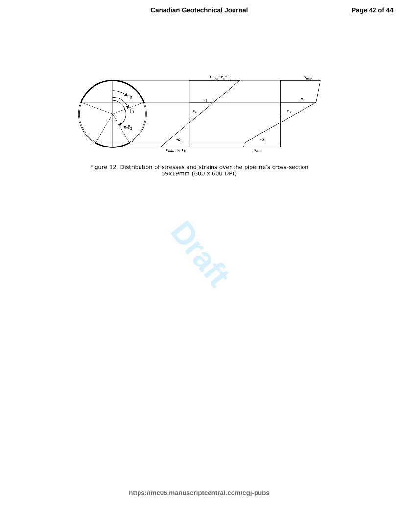
Figure 12. Distribution of stresses and strains over the pipeline’s cross-section.

Figure 13. Proposed methodology workflow.

Page 27 of 44



Draft

Appendix 1

The procedure employed to take into account the bilinear stress-strain relationship of the pipeline steel

(Figure 11) considers the exact distribution of stresses and strains on the pipeline’s cross-section, as a

function of the developing axial force and bending moment. More specifically, under the assumption that

the deformed pipe section remains plane, the total longitudinal strain distribution can be expressed as:

( ) a b cosε β = ε + ε β (A1)

where β is the polar angle of the cross-section, defined in Figure 12, while εa and εb are the axial and

bending strains, respectively. Bending strain εb is calculated from the maximum bending moment Mmax

as:

maxb

M D

2EIε = (A2)

The corresponding axial strain εa is calculated from the demand for the integral of stresses over the

pipeline section to be equal to the developing axial force. For the sake of simplicity, the axial force FA

developing at point A can be utilized for this purpose. Considering the bilinear stress-strain relationship

shown in Figure 11, the total stress distribution is given by:

( )( )

( )

1 2 1 1

1 1 2

1 2 1 2

0 σ + Ε ε − ε ≤ β < β

= Ε ε β ≤ β ≤ π − β−σ + Ε ε + ε β < β ≤

σ β

π

(A3)

where:

Page 28 of 44



Draft

1 a

b

1 a 1 a1,2

b b

1 a

b

1

arccos( ) 1 1

0 1

εε

ε εβ

ε ε

ε

επ < −

ε ε

= − ≤ ≤ ε

< ε

m

m m

m

(A4)

The corresponding axial force is therefore derived as:

( )( )( )

( )( )( )( )

1 a 1 2 1 2 a

1 2 1 2 10

1 2 1 2 b

E E ED t

F 2 t d t D t E E2

E E sin sin

π

β=

π − β + β−

= ⋅ σ ⋅ β = − +

ε

− β − β ε

− − β − β ε

− ε

∫ (A5)

The axial strain εa that satisfies the requirement F(εa)=FA can be calculated iteratively, starting from εao=0

and utilizing the Newton-Raphson method, as follows:

( )

ka a

k

a ak 1 k

a a

a

F F

dFd

+

ε =ε

ε −ε = ε −

ε

(A6a)

where:

( )( )( ) ( )

( ) ( )

1 21 1 2 1 2 1 2 a

a a

a 1 2 1 21 2 1 1 2 1 2 b

a a a a

d dE E E E E

d ddFt D t

d d d d dE E E E cos cos

d d d d

β βπ − − β + β − − + ε

ε ε = − ε β β β β + − − ε − − β − β ε ε ε ε ε

(A6b)

b 1,2

b 1,2

1,2 b 1,2

b 1,2a

b 1,2

b 1,2

1sin 0.01

sin

d 100 0.01 sin 0

100 0 sin 0.01d

10.01 sin

sin

± ε β ≤ − ε ββ − − < ε β ≤

= ± < ε β ≤ε

± < ε β

ε β

(A6c)

Page 29 of 44



Draft

Note that the limits in Equation A6c have been arbitrarily introduced in order to accelerate the

convergence procedure. The bending moment corresponding to εa and εb can be calculated as:

( ) ( )( ) ( )( )

( )( ) ( )( )

2

0

1 b2 1 2 1 2 a 1 2 1 2 1

1 2 1 2 b 1 2 1 2 b

D tM 2 t cos d

2

EE E sin sin E E sin sin

t t D 2

E E E E sin2 sin22

2 4

π

β=

− = σ β⋅ β =

π − − − β ε −ε

β +

ε ε

β + β ε − =

− β + β − β + β − −

∫

(A7)

This bending moment is not necessarily equal to the maximum developing bending moment Mmax utilized

in Equation A2. Therefore, in order to ensure compatibility between the applied force and bending

moment and the corresponding developing axial and bending strains, an equivalent secant Young’s

modulus is estimated and the analysis of the bend (i.e. Step 2) is repeated until convergence is

accomplished. The secant Young’s modulus for the each subsequent iteration is calculated on the basis of

moment M derived in Equation A7, as:

b

MDE

2I′ =

ε (A8)

Appendix 2

In order to facilitate the practical application of the proposed methodololgy, a schematic workflow is

presented in Figure 13.

Page 30 of 44



Draft

Figure 1. Definition of basic problem parameters 42x20mm (600 x 600 DPI)

Page 31 of 44



Draft

Figure 2. Decomposition of the pipeline into (a) a curved and (b) a straight segment 51x14mm (600 x 600 DPI)

Page 32 of 44



Draft

Figure 3. Definition of pipeline curved length L_c and unanchored length L_anch. 57x38mm (600 x 600 DPI)

Page 33 of 44



Draft

Figure 4. Structural model of the arched pipeline bend 75x65mm (600 x 600 DPI)

Page 34 of 44



Draft

Figure 5. Reduced structure loaded with (a) unit axial force FA=1, (b) unit shear force QA=1, (c) unit moment MA=1 and (d) soil resistance loads tu and qu

42x9mm (600 x 600 DPI)

Page 35 of 44



Draft

Figure 6. Elastic beam on elastic foundation: boundary conditions for (a) point A and (b) point B 69x56mm (600 x 600 DPI)

Page 36 of 44



Draft

Figure 7. Distribution of axial forces with distance beyond point B 40x18mm (600 x 600 DPI)

Page 37 of 44



Draft

Figure 8. Distribution of axial forces along the straight part of the pipeline 49x16mm (600 x 600 DPI)

Page 38 of 44



Draft

Figure 9. Comparison of analytical predictions (lines) against numerical results (points) 109x66mm (600 x 600 DPI)

Page 39 of 44



Draft

Figure 10. One-to-one comparison of analytical predictions against numerical results 59x19mm (600 x 600 DPI)

Page 40 of 44



Draft

Figure 11. Bi-linear stress-strain relationship of pipeline steel 58x39mm (600 x 600 DPI)

Page 41 of 44



Draft

Figure 12. Distribution of stresses and strains over the pipeline’s cross-section 59x19mm (600 x 600 DPI)

Page 42 of 44



Draft

Figure 13. Proposed methodology workflow. 191x202mm (300 x 300 DPI)

Page 43 of 44



Draft

Tables

Table 1. API5L-X65 steel properties considered in the parametric analyses.

Yield stress (σ1) 490 MPa

Yield strain ( ε1=σ1/E1 ) 531 MPa

Failure stress (σ2) 4.0 %

Failure strain (ε2) 210 GPa

Elastic Young’s modulus (E1) 0.233 %

Plastic Young’s modulus ( E2=(σ2-σ1)/(ε2-ε1) ) 1.088 GPa

Table 2. Soil spring properties considered in the analyses.

Yield Force

(kN/m)

Yield

Displacement

(mm)

Axial (friction) springs 40.5 3.0

Transverse horizontal springs 318.6 11.4

Page 44 of 44



Documents

Draft - University of Toronto T-Space · a curved pipeline bend of angle φ with a radius of curvature R is located at a distance L A from the point of PGD application on the pipeline