Embed Size (px)
Citation preview

1
DRAFT REPORT OF THE TEST METHOD VALIDATION
OF AVIAN ACUTE ORAL TOXICITY TEST – OECD DRAFT TEST GUIDELINE 223

2
TABLE OF CONTENTS
DRAFT REPORT OF THE TEST METHOD VALIDATION
OF AVIAN ACUTE ORAL TOXICITY TEST – OECD DRAFT TEST GUIDELINE 223
........................................................................................................................................................... 1
EXECUTIVE SUMMARY ............................................................................................................... 8
Introduction .................................................................................................................................. 10 2. History ..................................................................................................................................... 10
3. Rationale for the experimental design used in the draft Test Guideline 223 .......................... 11 4. Test description ........................................................................................................................ 12 5. Statistical simulations supporting the development and validation of the Draft OECD TG223 .
…………………………………………………………………………………………………..14 6. Instruments developed to enhance the reproducibility and user-friendliness of the guideline 16
6.1. Evaluation of clarity of the guideline through written quizzes ......................................... 16
6.2. Dose calculator – SEDEC (SEquential DEsign Calculator) ............................................. 17 7.0 Ring Test ............................................................................................................................... 17
7.1. Purpose of the ring test ...................................................................................................... 17 7.2. Outline of validation design .............................................................................................. 17 7.3. The criteria for the selection of chemicals used in the ringtest included the following .... 17 7.4. The criteria for evaluating results of the ring-test: ............................................................ 18
7.5. Participating laboratories ................................................................................................... 18
7.6. Results, evaluation and discussion of the ring test. Detailed tables in Appendix VI ...... 20 7.7. Evaluation of ring-test data in comparison with EPA historical Repeat data and result of
simulations performed .............................................................................................................. 21
Historic USEPA Bobwhite data performed to USEPA FIFRA 71-1 and the OPPTS guideline .. 23 Ring Test Data .......................................................................................................................... 23
How do the estimates of variance compare? ............................................................................ 23 Discussion of results of the evaluation: .................................................................................... 23 How do the ring test results compare with the simulations. ..................................................... 24
Conclusion of evaluation: ......................................................................................................... 24 7.8. Feedback from the laboratories that took part (including feedback on SEDEC). ............. 27 7.9. Experience gained to date with regulatory studies performed to draft OECD guideline 223
.................................................................................................................................................. 27
8. GLP status of the validation work ....................................................................................... 28 9. Availability for peer review................................................................................................. 28 10. Peer Review ........................................................................................................................ 28
Literature references .................................................................................................................... 29
APPENDIX I ................................................................................................................................... 30

3
STATISTICAL SIMULATIONS SUPPORTING THE DEVELOPMENT OF OECD DRAFT
TEST GUIDELINE 223 (TG223): AVIAN ACUTE ORAL TOXICITY TEST ........................... 30
Introduction .................................................................................................................................. 30 Method for Simulating Designs................................................................................................ 32
True LD50 and true slopes......................................................................................................... 32 Initial guess of the LD50 ........................................................................................................... 33 Dosing constraints .................................................................................................................... 33 Procedure for deciding whether a bird dies or survives ........................................................... 33 Procedure for selecting doses – standard 60-bird-one-stage design ......................................... 33
Procedure for selecting doses – original TG223 24-bird-3-stage design ................................. 33 Procedure for selecting doses – updated draft TG223 24/34-bird-3/4-stage design ................ 33 Working estimates of LD50 in difficult situations .................................................................... 34
Final estimates of LD50 and slope ............................................................................................ 34 Part 1: Performance of the updated draft TG223 design ............................................................ 34
Presentation of Results ............................................................................................................. 34 How does the updated draft TG223 design compare with the original TG223 and the one-
stage designs? ........................................................................................................................... 34 Three stages vs four stages ....................................................................................................... 35 Criterion for selection of the third stage ................................................................................... 35 Criterion for use of stage four .................................................................................................. 36 Conclusion ................................................................................................................................ 36
Part 2: Potential for Improving Performance of the Standard 60-Bird Design using a Range-
Finder ........................................................................................................................................... 36
Method ...................................................................................................................................... 36 Results ...................................................................................................................................... 37 Conclusion ................................................................................................................................ 37
Part 3: Robustness of Updated TG223 Design to Natural Mortality ........................................... 37
Method ...................................................................................................................................... 37 Results ...................................................................................................................................... 37 Conclusion ................................................................................................................................ 38
Part 4: Robustness of UpdatedTG223 Design to Delayed Mortality.......................................... 38 Method ...................................................................................................................................... 38 Results ...................................................................................................................................... 38
Conclusion ................................................................................................................................ 39 Part 5: Robustness of Updated TG223 to Inaccurate Initial Guesses of the LD50 ....................... 39
Method ......................................................................................................................................... 39 Results ...................................................................................................................................... 39 Conclusion ................................................................................................................................ 39
Part 6: Robustness of the Updated TG223 to Errors of Dosing................................................... 39
Conclusions .............................................................................................................................. 40
Appendix II – Validation of statistical simulations ..................................................................... 72 Validation of Simulations for the................................................................................................. 72
Draft OECD Test Guideline Avian Acute Oral Toxicity (TG223) ............................................. 72 Author: Carol Yarrow .................................................................................................................. 72 Date: 28
th March 2008 ................................................................................................................. 72
Summary ...................................................................................................................................... 72

4
Introduction .................................................................................................................................. 72 Description of Validation Process ............................................................................................... 72 Results of Validation Process ...................................................................................................... 73
3.1Step 1 ................................................................................................................................... 73
3.2Step 2 ................................................................................................................................... 75 3.3Step 3 ................................................................................................................................... 75
Comparison of Estimates of LD50 and Slope ........................................................................ 75 Comparison of Classification of Dose Response Data at the end of Stage 4 ........................ 78 Investigation of Differences in Results of Simulated Data ................................................... 79
Random Number Generation ................................................................................................ 79 To simulate the initial guess of the LD50. ............................................................................. 79 To simulate the number of dead birds at each dose at each stage: ........................................ 79 A note on SAS CALL routines: ............................................................................................ 80
Simulation of LD50 values ..................................................................................................... 80 Simulation of number of dead birds for each stage ............................................................... 81 Regeneration of simulated data using original programs ...................................................... 81
Conclusions .............................................................................................................................. 83 References ................................................................................................................................ 83
Annex I of appendix 2 Simulation results: ................................................................................. 84 Annex 2 of Appendix 2: Programs to validate SAS program, analysis.sas. .............................. 94
Annex 3 of appendix 2: Programs to validate SAS program, results.sas. ............................. 110
Annex 4 of appendix 2: Programs to validate SAS programs, stg12.sas, stg3.sas and stg4.sas.112 Annex 5 of appendix 2: Summary of investigation into seed behaviour in SAS ...................... 119
Consequences of using systematic seeds ................................................................................ 119 Appendix III – Evaluation of clarity of the guideline through written quizzes. ........................ 123
A. TG223 Avian Acute Oral Toxicity Test - Reading Comprehension Exam without answers
(March 2008) .......................................................................................................................... 124
TG223 Avian Acute Oral Toxicity Test - Reading Comprehension Exam with correct
answers (March 2008) ............................................................................................................ 127 C. TG223 Avian Acute Oral Toxicity Test - Results from First Quiz to Evaluate Guideline
Clarity (based on March 2007 draft, summary prepared September 2007) ........................... 131 D. TG223 Avian Acute Oral Toxicity Test - Results from Second Quiz to Evaluate Guideline
Clarity (based on March 2008 draft, summary prepared September 2009) ........................... 137
Ensure guidance is clear. Provide more clear examples.Appendix IV – Manual of SEDEC
programme and Example of SEDEC output .......................................................................... 143
Appendix IV – Manual of SEDEC programme and Example of SEDEC output .................. 144 SEDEC Manual ...................................................................................................................... 144
Appendix V ................................................................................................................................ 148
A. Verification of the sequential design calculator SEDEC: ..................................................... 148 Summary................................................................................................................................. 148
Introduction ............................................................................................................................ 148 SEDEC Setup using Windows Vista and Excel 2007 ............................................................ 150
Limit Tests .............................................................................................................................. 150 4.1 Tests of different mortality patterns .............................................................................. 150 4.2 Doses for Stage 2 and override maximum / minimum dose facility ............................. 153 4.3 Varying Limit Doses ..................................................................................................... 154 Stage 1 Setup ....................................................................................................................... 155

5
Sequential Testing: Stages 1 to 4 ........................................................................................ 156 Sequential Testing: Analyses of Test Datasets ................................................................... 156 Sequential Testing: Comparison of Results of Analyses of Test Datasets ......................... 157 Comparison of LD50 Estimates ........................................................................................... 161
Summary of Issues Identified .............................................................................................. 163 References ........................................................................................................................... 163
Post-Test Corrections and Additions to SEDEC ....................................................................... 182 Author: T. A. Springer, Wildlife International, Ltd................................................................... 182 Date: 29
th September 2009 ......................................................................................................... 182
C. Verification of Post Test Corrections and Additions to SEDEC .......................................... 193 Author: Carol Yarrow, Stats Matters ......................................................................................... 193 Date: 4
th October 2009 ............................................................................................................... 193
Appendix VI – Tables of results obtained by the ring test labs ................................................. 194
Lab 1: Substance A: MCPA Acid: Outcome of SEDEC Programme – Audit Trail ............. 197 Lab 1: Subtance A: MCPA Acid – Mortality table ................................................................ 198 Lab 1: Substance A: MCPA Acid – Body weight .................................................................. 199
Lab 1: Substance A: MCPA Acid – Food consumption......................................................... 200 Lab 1: Substance A: MCPA Acid .......................................................................................... 201 Lab 1: Substance A: MCPA Acid .......................................................................................... 201 Clinical Observations Stage 1: ............................................................................................... 201 Lab 1: Substance A: MCPA – Clinical observations – stage 1 ctd. ....................................... 202
Lab 1: Substance A: MCPA Acid .......................................................................................... 203 Clinical Observations Stage 2: ............................................................................................... 203
Lab 1: Substance A: MCPA Acid – Clinical observations – stage 2 ctd. .............................. 204 Clinical observations Stage 3: ................................................................................................ 204 Lab 1: Substance A: MCPA Acid – Clinical observations – stage 3, ctd. ............................. 205
Lab 1: Substance A: MCPA Acid .......................................................................................... 206
Clinical observations Stage 4: ................................................................................................ 206 Lab 1: Substance A: MCPA Acid – Clinical observations stage 4, ctd. ................................ 207 Lab 1: Substance B: Isazofos : Output of SEDEC programme .............................................. 208
Lab 1: Substance B: Isazofos : Output of SEDEC programme: audit trail ............................ 211 Lab 1: Substance B: Isazofos : Mortality table ...................................................................... 212 Lab 1: Substance B: Isazofos : Body .................................................................................... 213
1: Substance B: Isazofos : Food consumption ........................................................................ 214 Lab 1 – Substance B: Isazofos : Clinical observations........................................................... 215
Lab 1 – Substance B: Isazofos : Clinical observations........................................................... 217 Clinical observations stage 1 .................................................................................................. 217 Clinical observations stage 2 .................................................................................................. 217
Clinical observations stage 3 .................................................................................................. 218 Lab 1 – Substance B: Isazofos : Clinical observations........................................................... 219
Clinical observations stage 3 ctd. ........................................................................................... 219 Clinical signs stage 4 .............................................................................................................. 220
Lab 1 – Substance B: Isazofos : Clinical observations........................................................... 221 Clinical observations stage 4 ctd. ........................................................................................... 221 Lab 2: Substance A: MCPA Acid (no SEDEC output): Mortality tables .............................. 222 Lab 2: Substance A: MCPA Acid : Body weights ................................................................. 223 Lab 2: Substance A: MCPA Acid: Food Consumption.......................................................... 224

6
Lab 2: Substance A: MCPA: Clinical observations ............................................................... 225 Clinical observations stage 1 .................................................................................................. 225 Lab 2: Substance A: MCPA: Clinical observations ............................................................... 226 Clinical observations stage 1 ctd. ........................................................................................... 226
Lab 2: Substance A: MCPA: Clinical observations ............................................................... 228 Clinical observations stage 2 .................................................................................................. 228 Lab 2 Substance 2: MCPA Acid: Clinical observations ........................................................ 230 Clinical Observations stage 2 ctd. .......................................................................................... 230 Lab 2: Substance A: MCPA Acid: Clinical observations stage 3 .......................................... 231
Lab 2: Substance A: MCPA Acid: Clinical observations stage 3 ctd. ................................... 233 Clinical observations stage 4: ................................................................................................. 233 Lab 2: Substance A: MCPA Acid: Clinical observations stage 4 ctd. ................................... 234 Lab 2: Substance B: Isazofos: (No SEDEC output) Mortality ............................................... 236
Lab 2: Substance B: Isazofos: Body weights ......................................................................... 237 Lab 2: Substance B: Isazofos: Food consumption ................................................................. 238 Lab 2: Substance B: Isazofos: Clinical observations – stage 1 .............................................. 239
Clinical observations – stage 2 ............................................................................................... 240 Lab 2: Substance B: Isazofos: Clinical observations stage 2 ctd. .......................................... 241 Clinical observations stage 3 .................................................................................................. 242 Lab 2: Substance B: Isazofos – Clinical observations stage 3 ctd. ........................................ 242 Lab 3: Substance A: MCPA Acid: Outcome of SEDEC Programme ................................... 244
Lab 3: Substance A: MCPA Acid: Output SEDEC programme – Audit trail........................ 247 Lab 3: Substance A: MCPA Acid: Mortality data .................................................................. 248
Lab 3: Substance A: MCPA Acid: Body weights .................................................................. 249 Lab 3: Substance A: MCPA Acid: Food consumption .......................................................... 250 Lab 3: Substance A: MCPA Acid: Clinical observations stage 1: ......................................... 251
Lab 3: Substance A: MCPA Acid: Clinical observations stage 1, ctd.: ................................. 252
Clinical observations stage 2: ................................................................................................. 253 Lab 3: Substance A: MCPA Acid: Clinical observations stage 2, ctd. .................................. 254 Clinical observations stage 3: ................................................................................................. 255
Lab 3: Substance A: MCPA Acid: Clinical observations stage 3, ctd ................................... 255 Lab 3: Substance A: MCPA Acid: Clinical observations, stage 4, ctd .................................. 257 Lab 3: Substance A: MCPA Acid: Clinical observations, stage 4, ctd .................................. 258
Lab 3: Substance B: Isazofos: Output from SEDEC programme .......................................... 259 Lab 3: Substance B: Isazofos: Output from SEDEC programme – Audit Trail .................... 261
Lab 3: Substance B: Isazofos: Mortality data ......................................................................... 262 Lab 3: Substance B: Isazofos: Body weights ......................................................................... 263 Lab 3: Substance B: Isazofos: Food consumption ................................................................. 264
Lab 3: Substance B: Isazofos: Clinical observations – stage 1 .............................................. 265 Lab 3: Substance B: Isazofos: Clinical observations stage 1 ctd. .......................................... 266
Clinical observations stage 2: ................................................................................................. 266 Lab 3: Substance B: Isazofos: Clinical observations stage 2 – ctd. ....................................... 267
Clinical observations stage 3 .................................................................................................. 267 Lab 3: Substance B: Isazofos: Clinical observations stage 3, ctd. ......................................... 268 Lab 4: Substance A: MCPA – Acid: Output SEDEC Programme ......................................... 269 lab 4: Substance A: MCPA – Acid: Output SEDEC Programme .......................................... 270 Lab 4: Substance A: MCPA –Acid – Mortality data .............................................................. 272

7
Lab 4: Substance A: MCPA –Acid – Food consumption ....................................................... 273 Lab 4: Substance A: MCPA –Acid : Clinical observations stage 1: ...................................... 274 Lab 4: Substance A: MCPA –Acid : Clinical observations stage 1, ctd. ............................... 275 Clinical observations stage 2: ................................................................................................. 276
Lab 4: Substance A: MCPA –Acid : Clinical observations stage 2, ctd. ............................... 277 Clinical observations stage 3: ................................................................................................. 278 Lab 4: Substance A: MCPA –Acid : Clinical observations stage 3, ctd. ............................... 278 Lab 4: Substance B: Isazofos: Output SEDEC Programme ................................................... 280 Lab 4: Substance B: Isazofos: Output SEDEC Programme – Audit trail .............................. 282
Lab 4: Substance B: Isazofos: Body weights ......................................................................... 283 Lab 4: Substance B: Isazofos: Food consumption ................................................................. 284 Lab 4: Substance B: Isazofos: Clinical observations stage 1 ................................................. 285 Lab 4: Substance B: Isazofos: Clinical observations stage 1, ctd. ......................................... 286
Clinical observations stage 2 .................................................................................................. 286 Lab 4: Substance B: Isazofos: Clinical observations stage 2, ctd. ......................................... 287 Clinical observations stage 3: ................................................................................................. 287
Lab 4: Substance B: Isazofos: Clinical observations stage 3 ctd. .......................................... 288 Lab 4: Substance B: Isazofos: Clinical observations stage 4. ................................................ 289 Lab 4: Substance B: Isazofos: Clinical observations stage 4, ctd .......................................... 290
Substance A: MCPA Acid – Wildlife International, Ltd. project 222-101 – Performed in 1986:
Mortality tables .......................................................................................................................... 291
Substance A: MCPA Acid – Wildlife International, Ltd. Project 222-101: Body weight and
food consumption ................................................................................................................... 291
Substance A: MCPA Acid – Wildlife International, Ltd. Project 222-101: Body weight and
food consumption ................................................................................................................... 292 Substance A- MCPA Acid: Wildlife International, Ltd. Project 222-101: Description of
mortality and clinical observations ......................................................................................... 292
Substance A- MCPA Acid: Wildlife International, Ltd. Project 222-101: Description of
mortality and clinical observations ......................................................................................... 293 Substance B: Isazofos – Wildlife International, Ltd. project 108-223 – Performed in 1983:
Mortality tables ....................................................................................................................... 295 Subance B: Isazofos – Wildlife International, Ltd. project 108-223 – Performed in 1983:
Body weight and food consumption tables: ........................................................................... 297
Substance B: Isazofos – Wildlife International, Ltd. project 108-223 – Performed in 1983:
Description of mortalities and clinical observations. ............................................................. 297
Substance B: Isazofos – Wildlife International, Ltd. project 108-223 – Performed in 1983:
Description of mortalities and clinical observations. ............................................................. 298 Appendix VII – A. Studies from EPA data base used to evaluate ring-test results. ............. 303
Appendix VII – B: .................................................................................................................. 304 Appendix VIII – Example results of regulatory studies performed to date ........................... 319

8
EXECUTIVE SUMMARY
The acute oral toxicity of a substance to birds is core regulatory information for the registration of plant
protection products. OECD requested that an acute oral toxicity guideline for birds be developed that
would deliver an estimate of the LD50, slope and confidence limits, using as few birds as possible. The
draft TG223 guideline was developed in order to meet this request and describes a sequential design in
which cumulative responses at each stage are used to provide a working estimate of the LD50 and slope that
are used to set the doses for the next stage. After the final stage all responses are combined into a single
statistical analysis that determines an LD50, a slope and confidence limits.
The draft TG223 design is flexible in terms of the number of stages and birds. If available data suggest the
LD50 may be greater than 2000 mg/kg, a single stage limit test may be performed using 5 birds at the limit
concentration and 5 birds in the control group. If toxicity is expected, to be less than 2000 mg/kg a full
dose response test is performed using 3 or 4 stages (24 or 34 bird, respectively – excluding controls). In
the rare event the design does not result in an estimate of slope, then more stages (and birds) can be added.
Alternatively, if only the LD50 is required without an estimate of the slope and confidence limits the
numbers of birds tested may be reduced. This report addresses the validation of the full LD50 test design.
The performance of the design was evaluated through extensive computer simulations in which different
designs were compared to a 1-stage 60-bird design (similar to OPPTS850.2100). These simulations
indicated that draft TG223 would estimate the LD50 as well as the 60-bird design, but using substantially
fewer animals, and improve the frequency with which a slope is estimated. The computer program that
performed the simulations has been independently validated.
A multi-stage design is more challenging for test laboratories than a single stage study. In order to evaluate
the user-friendliness and clarity of the guideline a reading comprehension test was prepared. The results
and conclusions of the reading comprehension test quizzes are presented in the appendix and may be used
to assist in training of future draft TG223 users and were used to further improve the clarity of the
guideline. Secondly a sequential design calculator tool (SEDEC) has been developed in the form of a
Microsoft® Excel spreadsheet, in order to facilitate and aid in the selection of doses at each stage and to
estimate the LD50, slope and confidence limits. A report of the validation of this tool is included as an
appendix in this validation report. It will be made publicly available from the OECD website.
Ring testing was carried with two chemicals tested in each of five laboratories to confirm the results of the
statistical simulations. For each of these chemicals historical results were available for a standard fixed-
dose design as carried out to meet US EPA requirements (OPPTS850.2100). When comparing the results
of the ring test studies between laboratories and with the results of the original studies, the results appeared
similar. Two statistical comparisons were made. In the first, the variability in LD50 calculations and slope
estimates was compared with the variability found in these endpoints in a selection of 15 repeat studies
from the EPA data base. The LD50 estimates from the ring-test showed less variability than the EPA repeat
studies. The variability in slopes from the ring-test data was higher than that seen in the EPA repeat
studies. The latter can be explained by the higher frequency with which slopes are determined in the draft
TG223 design when the slope is steep, than in the EPA data base studies. In the second, the variability in

9
LD50 and slope estimates observed in the ring-test data were compared with the variability predicted by the
computer simulations and shown to be similar.
The Validation Management Group concludes that the performance of draft TG223 delivers regulatory
endpoints of LD50, slope and confidence limits to a high standard while reducing the numbers of birds
tested. It is the Validation Management Group‘s recommendation that the guideline be published by OECD
as a final document.

10
Introduction
The acute oral toxicity of a substance is core regulatory information on safe use in labelling and risk
assessment in OECD member countries. OECD guidelines have a strong emphasis on animal welfare and
there are incentives and opportunities to refine the design to reduce animals tested. The avian acute oral
toxicity test guideline (draft TG223) has been in development since 1994 when OECD first requested an
acute guideline that substantially would limit the numbers of animals used . Draft TG223 describes a
sequential design where the responses at each stage are used to position the next set of doses for the
purpose of identifying the LD50, slope and confidence limits. The responses from all stages are combined
for final estimates of these parameters. The performance of the design initially was evaluated through
extensive statistical simulations comparing different designs with a 1-stage 60-bird design (similar to US
EPA OPPTS850.2100) and an ‗up-down procedure‘ (similar to TG425 for mammals) These simulations
indicated that Draft TG223 would estimate the LD50 as well as the 60-bird design, using substantially fewer
animals. The simulations also indicated that the frequency with which a slope estimate can be achieved,
would be increased. It is possible to guarantee a slope estimate by adding additional stages beyond those
prescribed in the design to generate reversals and partial responses. To aid the selection of doses at each
stage and to estimate the LD50, slope and confidence limits, a SEquential DEsign Calculator tool (SEDEC)
has been developed as an Excel 2000® spreadsheet that will be publicly available from the OECD web site
for use with the final TG223 guideline.
The draft TG223 of March 2007, reflected the consensus obtained after all the concerns raised in member
country comments and by members of the expert group had been addressed. In 2007 a validation plan was
approved by OECD of which the results are presented here. This validation report includes:
Background information on the guideline and its development;
Results of the statistical simulations, their validation and an account of how all the concerns
raised were addressed;
A summary of the computer programme developed to estimate the LD50 and provide doses for
each stage of the test (Sequential Design Calculator: SEDEC);
The results and conclusions of a reading comprehension test performed to ensure readability and
clarity of the guideline;
The results and discussion of the ring test performed with two chemicals at several different
laboratories;
Summary and evaluation of feedback received from participating laboratories.
Examples of (regulatory) TG223 studies conducted with the draft guideline to date.
2. History
Work on the development of an OECD guideline for acute oral testing in birds started during a workshop
on Avian Toxicity Testing was held in Pensacola, Florida, United States on the 4-7 December 1994. 1)
The workshop comprised 48 wildlife toxicology specialists from 10 countries including 27 from North
America and 18 from Europe. This workshop was part of the OECD‘s Pesticide Programme and had the
following objectives: i) to confirm which tests are critical for risk assessment; ii) to evaluate the positive
and negative features of existing test methods and alternatives against critical required features; iii) to

11
revise or develop OECD test guidelines for avian toxicity testing as needed, while minimising the numbers
of animals required for such tests. The workshop recommended that an acute oral toxicity guideline should
describe a limit test design for chemicals of low toxicity, a definitive LD50 test that provided a dose
response slope and confidence limits and a short version to provide an approximate LD50 where the
toxicity to additional species was required to investigate the species sensitivity distribution (SSD). To
achieve this with least numbers of animals it was agreed to focus on mortality as the primary endpoint with
no attempt to determine a NOEL for other outcomes. Further it was agreed that setting doses to achieve
other parameters compromise the dose response for mortality. The Workshop also identified some areas of
work that were necessary to support a new acute oral toxicity guideline, including the identification of the
most efficient design to estimate the LD50 and slope using the least number of birds.
These actions were taken forward by an OECD Expert Group at open and closed meetings at SETAC in
Europe and the United States. In 1998 a draft guideline was prepared for OECD that described a limit test,
an Up-and-Down test and a Dose response test. Following discussions within OECD the avian expert
group was asked to re-evaluate the test design to reduce the number of animals further. The group had to
balance the need for reducing the numbers of animals in the test with the requirement to fulfil the
regulatory need to provide an LD50 and slope estimate. OECD requested that the group work with
statisticians to develop a suitable design. As a consequence a team of statisticians prepared a plan to
evaluate several designs with different numbers of stages and birds per stage through extensive computer
simulations. The selected multi-stage design allowed a significant reduction in required individuals needed
while assuring ability to estimate both an LD50 and a slope were estimable. The draft guideline was
submitted again to OECD in 2002 and given the reference TG223. As part of the subsequent commenting
round, a number of specific concerns were raised. The key issues included: i) whether or not to use
controls; ii) which test species to apply the design to; iii) whether or not to randomly select birds,
irrespective of their sex; iv) the impact of delayed or background mortality on the estimate of the LD50.; v)
how to evaluate endpoints other than mortality. All the issues raised were resolved at public (SETAC)
meetings and closed (OECD) meetings. Further questions were put to the Expert Group by representatives
of USEPA and these were addressed with the help of the US EPA biologists and statisticians. A third
revision was prepared and submitted to OECD for further commenting in 2007. A detailed account of the
concerns raised and the changes subsequently made is presented in appendix I of this report.
Following the OECD member-country commenting round it was recommended that a validation plan be
prepared and conducted. A validation plan was prepared and submitted to OECD in 2007. The elements of
this plan were completed in 2009 and is reported in this document. Ring testing was conducted for the
LD50-slope test only.
3. Rationale for the experimental design used in the draft Test Guideline 223
The Draft TG223 design is flexible in terms of number of stages, and therefore in terms of number of birds.
First of all, if available data suggest the LD50 may be greater than 2000 mg/kg, a single stage limit test may
be performed using five birds at the limit concentration and five birds in the control group. If toxicity is
expected, a full dose response test (LD50 – slope test) is performed. If the 3 stage (24 bird) or 4 stage (34
bird) design does not result in an estimate of slope, then more stages (and birds) can be added.
Alternatively, if the slope and confidence limits are not required the numbers of birds tested may be
reduced by using the LD50-only test. This validation report only addresses the validation of the full LD50
test design.
The LD50 – slope test is a sequential design using 24-34 individuals (excluding controls) to estimate the
LD50, slope and confidence limits. This is achieved by the calculated placement of doses for single or
small groups of birds/dose to provide a working estimate of the LD50 and slope. This is used in turn to
define the placement of doses and the number of animals per dose in the next stage until a final estimate of

12
the LD50 and slope are determined by combining all stages. Sequential designs can be used where there is
low expectation of drift (the responses changing in time) and none to extremely low background mortality. a) Both these factors have been shown to be low over short intervals (days) using robust species under
controlled experimental conditions. Under these conditions the responses may be combined across stages
and controls limited to a single stage. 1
A stopping rule, linked to the number of reversals or partial mortalities at a single dose, is incorporated into
the design. This prevents the unnecessary use of animals once an adequate estimate of the LD50,slope with
confidence limits are met. A reversal is an instance when percent mortality at a given dose is higher than
the percent mortality at the next higher dose. Partial mortality is an instance where only a proportion of
birds die at a given dose. The range over which reversals and partial mortalities occur provides information
about the LD50 and slope.
Doses are not selected for determining NOELs and there is no requirement to estimate NOELs through
statistical analysis. Information on non-lethal endpoints like food consumption and bodyweight are
collected for qualitative evaluation.
A control group is five birds for both the limit test and the sequential (LD50--slope) test. For laboratory-
reared avian species, historical data have demonstrated that background mortality is very low.
4. Test description
The test is divided into a number of discrete stages. At each stage in either the LD50-slope or the LD50-only
test designs, one or more birds are given a single oral dose (mg/kg body weight) of the test substance using
doses that are expected to bracket the evolving working estimate of the LD50. Birds are observed for 14
days, but selection of doses for subsequent stages is typically based on observed mortality and toxicity
symptoms after three days. This interval may be reduced early in the test if mortality or signs of recovery
occurs quickly, or the interval may be extended if delayed mortality is expected or observed.
The sequential test can be initiated using information gained from a failed limit test (one or more
mortalities at the limit dose – see Figure 1 of the draft TG223). For compounds of suspected high toxicity,
testing may be initiated in Stage 1 where each of four birds is given a different dose, so that doses cover
the best available estimate of the LD50 (e.g., based on the rodent or other bird species‘ LD50). Using the
outcome of Stage 1, the doses that bracket the working estimate of the LD50 are determined for Stage 2,
and at each of ten doses, one bird is dosed. If there is a working estimate of the LD50 available from a
failed limit test, the sequential test may start with Stage 2. The process continues to Stage 3 and possibly to
Stage 4 (detailed stopping rules are given in the test guideline).
Individually-caged young adult birds are acclimated to experimental conditions before being randomly
allocated to receive an oral gavage dose. Dosing procedures, test conditions and animal husbandry
methods are described and are consistent with US EPA OPPTS850.2100. The recommended strategy for
testing materials that are unlikely to present a significant hazard is to perform a test with multiple birds (5)
dosed at the limit dose. If toxicity is expected, the recommended strategy is to use a sequential (staged)
design (see Figure 2 of the draft TG223). Stages 1 and 2 require non-replicated doses, while Stages 3
and 4 require replicated doses. In Stage 1, the range of doses is based on the best available estimate of the
LD50 (e.g., the rodent LD50). Doses for subsequent stages are determined based on the mortalities observed
in all previous stages.
1 An evaluation of background mortality recorded in 4 different laboratories is taken up into the simulations report in Appendix I
of this report.

13
After dosing, the birds are observed for a 14-day period in order to record mortality and sublethal effects.
It may be necessary to extend the observation period if there is evidence of delayed effects. The data
collected in the first three days of a stage usually supply sufficient information to determine whether birds
are likely to recover from effects encountered, or whether additional mortality will occur. If day 3
indicates that further mortality may occur in a test stages, the calculation of the working estimate may be
delayed until recovery of the remaining test birds is evident. In some cases it may be necessary to wait for
up to 14 days before moving to the next stage. Calculation of the working estimate on day 3 of a test
stages allows the full test and all dosing to be completed over a relative short time frame. For example, the
total length of the study would be 21 days if (1) three stages were required to estimate and LD50 and slope,
(2) 14-day observation period were sufficient and (3) three days was a sufficient time period for
determination of doses for the subsequent stage.
The guideline provides information for selecting doses at each stage, that bracket the evolving working
estimate of the LD50. In addition a SEquential DEsign Calculator (SEDEC) will be made available on the
OECD website that estimates the working LD50 at each stage, identifies the doses for the next stage and
calculates the final estimate of the LD50, slope and confidence limits.
Mortality is the primary endpoint in this study and background mortality is presumed to be negligible.
Controls are required to monitor the health and husbandry of test birds to ensure the study results provide
reliable results. Five untreated control birds from the same hatch will be included in the test. Control birds
will be sham dosed with the same carrier (or capsule) used with the test substance, and will be maintained
under the same conditions as treated birds. Control birds will be weighed prior to dosing as well as 3, 7,
and 14 days after dosing. Sham dosing will be performed on the same day as the first dosing with test
substance (either with the limit test if it is performed, or with Stage 1 of the sequential test). If
circumstances require the use of birds that are from a hatch different from the one used to start the test, an
additional control group of five birds from the second hatch must be included on the day that these birds
are used.
Clinical observations, body weights and food consumption are to be recorded throughout the study. During
the test, animals obviously in pain or showing signs of severe distress should be euthanised. The design
aims to minimise the use of test animals as shown in the table below:

14
Table 1: Number of animals required in the limit test and at each stages of the sequential design.
Test stage Treatment Control1
Limit test 5 5
1st stage if necessary 4 5
2nd
stage if necessary 10
3rd
stage if necessary 10
4th stage if necessary 10
1 5 birds in a limit test or 5 birds in a dose response test
The Limit Test , LD50only Test and LD50—slope use 10, 24 and 34 birds, respectively, excluding controls.
If the dose response curve is steep (fewer than two reversals or partial kills) at stage 3 and the slope cannot
be determined it may be necessary to go to a 4th stage (34 birds ex controls). The frequency with which the
investigator needs to progress to stage 4 is expected to be low.
Clinical observations, body weights and food consumption are to be recorded during the study.
5. Statistical simulations supporting the development and validation of the Draft OECD TG223
Computer simulations of draft designs have been used to compare the performance of standard 60-bird
one-stage designs (similar to that outlined in the current EPA guideline OPPTS 850.2100) to the original 3-
stage and the updated 3-stage and 4-stage draft TG223 designs, as explained below.
Appendix I contains a detailed report of the statistical simulations that evaluate the performance of three
types of design:
Single stage design with 50 birds. Two alternatives to the standard design, based on the OPPTS
850.2100 design.. The standard design comprises 5 doses, each of which is allocated to 10 birds
plus an untreated control of 10 birds. However, in this report, two alternatives to the standard
design have been evaluated, both of which have 10 doses with 5 birds per dose. In an earlier
evaluation both of these alternative designs were found to be superior to the design with 5 doses.
One of the design alternatives has a high/low dose ratio of 20 and is better for estimating slope; the
other has a high/low dose ratio of 50 and is better for the LD50.
3-stage sequential design with 24 birds. This is the original draft TG223 sequential design
recommended in a draft OECD guideline issued on October 2002. This design uses 3 stages: 4
non replicated doses in the first stage, equally spaced (on a log scale) around a provisional estimate
of the LD50; 10 non-replicated doses in the second stage, equally spaced (on a log scale) around an
updated estimate of the LD50; and 2 doses, each given to 5 birds, in the third stage.
4-stage sequential design with 34 birds. The updated version of the draft TG223 sequential design
as described in section 4 was also evaluated. After further simulations, it was discovered that the

15
original 3-stage design was unsatisfactory in certain situations, particularly when the true slope of
the dose response is steep. The original design has therefore been modified by the inclusion of an
alternative Stage 3, the use of which depends on the outcome of Stage 2, and an optional Stage 4,,
the use of which depends upon the outcome of the new alternative stage 3.
Each of the above designs was evaluated by means of computer simulation. For each design nine thousand
computer experiments were carried out, one thousand for each of nine combinations of true LD50 (5, 50,
and 1500 mg/kg) and true slope (2, 5, and 10). Appendix I describes the methods used to carry out the
simulations, to estimate the LD50 and slope for each computer-generated experiment, and to present the
results. The report in Appendix I also covers all of the concerns that have been raised in the course of the
development of the guideline and describes how these concerns were addressed through further simulation
testing and which protocol modifications were needed.
The conclusions from the simulation exercise were as follows:
For estimation of the LD50, all four designs compared in this report give a similar performance.
However, the Draft TG223, original and updated, designs require far fewer birds - either 24 or 34 -
so should be preferred.
For estimation of slope, the updated draftTG223 24/34-bird-3/4-stage design significantly
outperformed the other designs. It was successful (at least 80%) in estimating the slope even when
the true slope was steep. The original TG223 was less successful.
The updated draft TG223 has been presented as a 3- or 4-stage design, in the interests of
conserving animals. However, the principal of extending the number of stages can easily be
applied to 5 or more in any rare circumstances where this might be considered necessary.
In addition to this major conclusion, further simulations were able to show the following:
The performance updated Draft TG223 design is not noticeably affected by natural mortality. The
updated draft TG223 design is therefore robust when considering natural or background mortality
of 1% or less, which is typical of what is observed in practice in control birds. Appendix I of this
report provides a historical overview, performed in 2004, of control mortality recorded in
laboratories performing avian studies.
The performance of the updated draft TG223 design can be affected by delayed mortality (i.e.
mortality that occurs more than three days after treatment. However, the flexibility in the design
through the ability to increase the number of days between successive stages, the ability to repeat
stages and to increase the total number of stages allows the experimenter to mitigate the effects of
delayed mortality without the need to repeat a study.
The performance of the updated draft TG223 design is not noticeably affected by a poor initial
guess of the LD50, since correction at later stages can take place.
The effect of errors in dosing on the performance of the updated draft TG223 design is entirely
predictable and does not permit discrimination between competing designs.
As part of this validation excercise, an independent consultant has verified the simulation code by
independently developing and executing the code to repeat the original simulations. In addition, the
procedures used to tabulate and evaluate the simulation results were repeated independently. The report of
this work and reposes by the Expert group, is included as Appendix II of this report. One small finding
mentioned in the validation report, led to a correction of the original simulation programmes. Upon
rerunning the programmes small differences from the original runs were found. However, the response of

16
the expert group was that this does not change the conclusions from the simulations in any way. Not does it
have any implications for the design specified in the draft TG223 guideline.
6. Instruments developed to enhance the reproducibility and user-friendliness of the guideline
6.1. Evaluation of clarity of the guideline through written quizzes
As part of the validation process for the draft TG223, the Expert Group has conducted a reading
comprehension evaluation with written quizzes to evaluate clarity of the draft guideline language and to
help ensure that laboratories conducting the study will interpret the Guideline in an identical manner. An
eight question quiz (multiple choice and short answer) was developed based on the March 2007 version of
the draft TG223 Draft Guideline. Four biologists from EFED (US EPA/Office of Pesticide
Programs/Environmental Fate and Effects Division) volunteered to read the draft guideline and take the
quiz in August 2007.
Based on the results of these quizzes and National Coordinator comments submitted in summer 2007, the
draft guideline was edited and re-submitted to OECD in March 2008. The quiz was re-administered based
on the March 2008 revisions. All questions in the second quiz were the same as in the first quiz, with the
addition of one question focusing on identification of reversals and partials in hypothetical study data.
Several EFED biologists re-took the quiz using the 2008 draft guideline. In addition, EFED biologists,
independent testing laboratory employees who regularly conduct avian toxicity tests, and one avian
toxicology researcher took the quiz using the revised 2008 draft guideline. A copy of the quiz given for the
2008 draft guideline, a copy of the solutions, and summaries of results from the first and second round of
quizzes are provided in Appendix III.
For the first round based on the 2007 draft guideline, the respondents had difficulty identifying reversals in
sequences and following the concepts of moving through the stages. For example, they were unable to
identify if a study should move to Stage 3a or 3b based on results from Stages 1 and 2.
The second set of quiz-takers (2008 draft guideline) was a much larger group of 13 individuals with more
diverse backgrounds. However, no one in this group was able to respond correctly to all questions. Those
respondents who provided answers based on both the 2007 and the 2008 draft guidelines (three
individuals) felt the revised draft was better organized and much clearer. There were several questions
where the percentage of correct responses increased dramatically. For example, only two of the four
individuals evaluating the 2007 draft were able correctly to identify the number of reversals in the four
simple sequences provided in question 1. To address this concern, example sequences identifying partials
and reversals were added to the 2008 draft. When tested on the new draft, all 13 respondents correctly
identified the number of reversals in question 1. As another example, in 2007 only one of four individuals
correctly answered question 5 (identifying doses for stage 2 based on results of a limit test); however, nine
of 13 were able to correctly answer this question based on the 2008 draft guideline.
These improvements in correct response rate indicate that the draft guideline implemented in 2008 greatly
increased comprehension of the study design. However, some questions still had poor correct response
rates. This indicated that the guideline text would benefit from further revision focusing on clarity. This
has been done and is reflected in the final draft of the guideline, that is being circulated together with this
validation report. These results also substantiate the importance of providing to users of the draft TG223
guideline software that determines dose concentrations and performs LD50 calculations.

17
6.2. Dose calculator – SEDEC (SEquential DEsign Calculator)
SEDEC is an EXCEL® workbook designed to aid in dose selection and analysis of avian acute oral
toxicity studies performed in accordance with draft TG223. Facilities are provided for the user to enter
basic study information and to guide the user through the sequential calculations and selection of doses.
After a study is completed, SEDEC can calculate the LD50, dose response slope, and confidence intervals
for both. SEDEC provides facilities for printing reports of the study results, and also provides a secure
audit trail that records entry and changes to data, user decisions, the identity of the individual making
entries or decisions, and the date of the action or entry.
SEDEC (designed by Dr. Timothy Springer, Wildlife International, Ltd.) was made available to all
participating laboratories prior to starting the in-life phase of the ring testing. This calculator was not
available for the written quizzes (Chapter 6.1), since participants were requested to have full understanding
of and be able to perform all calculations themselves. This programme has been validated and the
validation report is included as Appendix V of this report.
7.0 Ring Test
7.1. Purpose of the ring test
To demonstrate the applicability and practicality of the test design described in the draft TG 223
at avian testing laboratories that perform avian testing.
To provide estimates of the LD50‘s and slopes and their respective confidence limits using the
draft TG223, in order to compare with LD50‘s and slope estimates from previous OPPTS-design
studies performed with the same chemicals (performed to FIFRA guidelines).
To support the validity of conclusions drawn on variability and bias of LD50 and slope estimates
in previously performed simulation-based assessments done using the tests performed according
to draft TG223.
To qualitatively compare information on sublethal endpoints from TG 223 with information from
historic OPPTS (FIFRA) studies.
7.2. Outline of validation design
Testing was performed with northern bobwhite quail. Two chemicals were tested in each of 5 laboratories
in order to allow an assessment of the combined effects of inter- and intra-laboratory variation, for
comparison with existing OPPTS-design studies in the EPA acute toxicity database. The size of the ring-
test design was a compromise to minimise the use of animals and resources. Ring-test results were put to
optimal use by comparing the uncertainty range found in the ring test results with that predicted from the
simulation results.
7.3. The criteria for the selection of chemicals used in the ringtest included the following
With each of the chemicals at least one OPPTS study with good performance parameters
(expressed as LD50 and slope with their respective confidence intervals) had to be available;
It is considered that the new guideline had to be shown to perform well for chemicals with
toxicities and different slopes. Hence one chemical (MCPA Acid) had a steep slope and was of
low toxicity and one chemical had a shallow slope (isazofos) and was of high toxicity in the
previously performed OPPTS-design studies;

18
Permission needed to be obtained from the pesticide manufacturer, therefore chemicals of
obvious commercial sensitivity were not included.
The chemical had to be stable in a vehicle. This was the case for both chemicals selected.
Chemicals that caused regurgitation in birds were avoided. No regurgitation was reported in
either of the original studies. Regurgitation was observed for both one chemicals at ring-test lab
no. 1 only.
The ring-test was performed using the same carrier and similar particle size as was used in the
original OPPTS-design studies.
7.4. The criteria for evaluating results of the ring-test:
For the selected chemicals, studies of the traditional design were available that showed good design
performance. The LD50, slope and confidence limits were estimated from the existing studies.
Evaluation of the results of the ring-test included:
A comparison between the estimates of LD50 and slope obtained from the ring test
studies and those obtained from the OPPTS-design studies. This was achieved through
visual inspection of the results in Table 2 combined with insights obtained from the
computer simulations (see chapter 5).
A comparison of within-chemical variability inestimates of LD50 and slope observed from the
ring-test data and variability observed in historic repeat studies using OPPTS-820.2100 and its
precursor US EPA FIFRA Guideline 71-1.
A comparison between the within-chemical variability in estimates of LD50 and slope
observed in the ring test data and variability observed in the simulations described in
Appendix I.
7.5. Participating laboratories
Participating laboratories were:
BASF (Germany) : contact Sabine Zok
Bayer Crop Sciences (US): contact: Mark Christ
Huntingdon LifeSciences (UK): contact David Cameron
Springborn Smithers (US): contact Larry Brewer
Wildlife International, Ltd. (US): contact Joann Beavers / Patrick Hubbard
The laboratories have been given a number so that results cannot be related to a particular laboratory.
Note: Upon finalisation of this draft validatin report results had not yet been obtained from one of the five
laboratories. If at all possible results from this laboratory will be incorporated into the report before its
finalisation.

19

20
7.6. Results, evaluation and discussion of the ring test. Detailed tables in Appendix VI
Table 2. Summary of validation ring-test results
Substance A: MCPA
Lab ID LD50 (95% CI)
(mg/kg bw)
Slope (95% CI) Number of
stages used
Number of birds used
Lab 1 1)
437 (360- 538) 9.67 (3.66 – 15.7) 4 34 + 5 controls
Lab 2 2) 3)
438 (338-544) 3.21 (1.26 and 5.16) 2)
4 34 + 5 controls
Lab 3 333 (280 – 400) 13.2 (4.3 – 22.1) 4 34 + 5 controls
Lab 4 554 (396-845) 6.22 (1.73-10.7) 4 34 + 5 controls
Lab 5 4)
Historic (FIFRA 71-1) study 377 (314-452) 11.6 Single stage
study
60 (including controls)
Substance B: Isazofos
Lab ID LD50 (95% CI)
(mg/kg bw)
Slope (95% CI) Number of stages
used
Number of birds used
Lab 1 1)
27.4 (0 and
infinity)
Could not be
estimated 5)
4 34 + 5 controls
Lab 2 2) 3)
24.4 (17.1 – 37.6) 3.3 (0.59 and 6.03) 2)
3 24 + 5 controls
Lab 3 16.1 (11.7 – 23.3) 7.7 (1.99 – 13.4) 3 24 + 5 controls
Lab 4 13.8 (10.4-17.4) 6.45 (2.57-10.3) 4 34 + 5 controls
Lab 5 4)
Historic (FIFRA 71-1) study 11.1 (8.3 - 14.7)
4.68 Single stage study 80 (including controls)
1) Some regurgitation was seen in the birds in this study, however, it does not appear to have impacted the results of the study, when comparing the LD50 values to those obtained
by the other laboratories. 2) This laboratory performed the studies without using SEDEC. The doses selected were run with SEDEC to obtain estimates for the purpose of comparative evaluation of the ring
test results. 3) A common control group was used for MCPA and isazofos 4) Results from this laboratory had not been received at the time of finalisation of the draft validation report. 5) This study went to 4 stages and had no reversals and no partial mortalities. In this case it was not possible to estimate the slope.

21
In paragraph 7.1 of this report 4 main purposes of the ringtest have been outlined. The first one, which is to
demonstrate the applicability and practicality of the test design described in Draft guideline 223 in typical
contract laboratories that perform avian testing, has been met by this ring test. The validation management
group asked for feedback from the laboratories on the method. While there were concerns raised by the
laboratories, as presented in chapter 7.8, all laboratories were able to perform the test without much
difficulty.
The second aim of the ringtest was to provide estimates of the LD50s and slopes and their respective
confidence limits for two chemicals. This was achieved and results are presented in Table 2. The results
obtained in the ringtest in terms of LD50 were comparable to the original studies performed by Wildlife
International, Ltd. using a single stage design like OPPTS 850.2100. For MCPA, the confidence limit
ranges for both the LD50 and the slope overlap with the confidence limits ranges for all of the ring-test
results. For Isazofos, the confidence limit range for the slope estimate for the OPPTS study overlaps with
the confidence range exhibited by three of the ring-test studies. While the estimates of the LD50 were
comparable between the labs, the confidence range for the historical study is outside the range exhibited by
four ring test studies, however confidence limit ranges show an overlap with labs 3 and 4. Lab 1 had no
confidence limits around its LD50 and hence no comparison could be made. A discussion of the variability
found in the slopes in the ring-test is given in Chapter 7.7.
Chapter 7.7 also deals with the comparison between the variability of data obtained in this ringtest and the
variability found in a sample of repeat tests taken from the EPA data base. Chapter 7.7 also deals with the
third aim of the ringtest. This aim was to see if the ring-test data would support the validity of previously
performed simulation-based assessments made of the variability and bias of LD50 and slope estimates from
tests performed according to the updated draft to TG223.
The final aim of the ring test was to qualitatively compare information on sublethal endpoints from TG 223
with information from historic OPPTS studies. To this end all findings related to bodyweights, food
consumption and clinical signs from the ring-test studies and from the original studies have been included
in Appendix VI of this validation report. A direct comparison of clinical observations recorded in the
different studies is difficult owing to the wide range of terminology used to describe the findings in the
respective studies.
No regurgitation occurred in either of the original studies. Some regurgitation was seen in birds from Lab
1, however this was not seen in birds from any of the other laboratories. One possible explanation may
have been a difference in dosing methodology, capsule dosing and intubation.
7.7. Evaluation of ring-test data in comparison with EPA historical Repeat data and result of
simulations performed
This section describes the following:
The statistical estimation of the variance for both LD50 and slope from a historic USEPA
data base (http://www.ipmcenters.org/Ecotox/index.cfm).
The estimation of variance for both LD50 and slope from the ring test data.
A comparison of the variances (i.e. historic versus ring test) via formal statistical tests.
Any statistically significant outcomes will be discussed in terms of expectations derived
from the simulation exercise in Appendix I.

22
Finally the variation (in LD50 and slope) observed in the ring test will be compared with
estimates obtained in the simulation studies in Appendix I. Since the results of the
simulation exercise are presented in terms of Box-Whisker plots, the uncertainty
intervals (see below) estimate from the ring test will be compared with the range shown
in the simulation studies.

23
Historic USEPA Bobwhite data performed to USEPA FIFRA 71-1 and the OPPTS guideline
Data, which is presented in Appendix VII, comprises 15 chemicals, and 32 individual LD50 values. Two
chemicals have 3 values each. The remaining chemicals have two values each. The data includes relatively
few estimates of slope because the OPPTS design is poor at estimating slopes. It is assumed that repeat
tests in a chemical are nested withing chemicals. Under this assumption a random effects-model can be
used to estimate both the variance between repeats and the variance between chemicals. Repeat tests on a
chemical may, or may not have been performed at the same lab as the original test. Therefore the variance
between repeats includes both intra- and inter-lab variability.
The between-repeat, within-chemical, estimate of variance for log10(LD50) is 0.062, with 17 degrees of
freedom. The within-chemical, between-repeat, estimate of variance for slope is 2.21, with 3 degrees of
freedom. Very approximate uncertainty intervals around three values for LD50 (i.e. LD50 = 5, 50, 1500)
have been computed as LD50 +/- 2*(standard deviation). These are shown in Table 3. Similarly,
approximate uncertainty intervals around 3 values for slope (i.e. Slope = 2, 5, 10) have been computed.
These are shown in Table 5. These values of LD50 and slope correspond to the values of LD50 and slope
that were used for the computer simulation component of the design validation.
Ring Test Data
Data comprises two chemicals and eight data values – four repeats for each of the ring test chemicals.
Again, it is assumed that repeat tests are nested within chemicals, so the form of analysis carried out was
the same as for the historic EPA data.
The between-repeat, within-chemical, estimate of variance for log10(LD50) was 0.014 with 6 degrees
freedom. The within chemical between repeat estimate of variance for slope is 13.240 with 5 degrees
freedom. Using 2*(standard deviation), very approximate uncertainty intervals were computed for three
values of LD50 (i.e. LD50 = 5, 50, 1500) (Table 4). Similarly, approximate uncertainty intervals around 3
values for slope (i.e. Slope = 2, 5, 10) have been computed (Table 5).
How do the estimates of variance compare?
For LD50: The variance ratio was computed with the larger estimate of variance as the numerator. In this
case the variance estimated from the EPA data was larger. This gave a value of 4.52 with 17 and 6 degrees
of freedom. The F-test single-sided p-value for this ratio is 0.035. This is statistically significant.
For Slope: The variance ratio is 5.99 on 5 and 3 degrees of freedom. In this case the variance estimated
from the ring test data was larger. This gives a one-sided p-value of 0.036, which also is statistically
significant.
Discussion of results of the evaluation:
For LD50, the variance from the EPA data is 4.52 times greater than the variance from the ring test.
Upon consideration, this outcome is not surprising since the simulations shown in Appendix I show, for

24
larger values of true slope, that variation between estimates of LD50 from draft TG223 is smaller than
variation between estimates from the ―OPPTS‖ design.
For slope, the variance of the ring test data is six times greater than the EPA data and the F-test does
confirm a significant difference. This result is consistent with the results of the simulation exercise where
the simulations for draft TG223 are more successful in estimating the slope. (see figures 1.4, 1.5 and 1.6 in
Appendix I). For shallow and medium slopes (slope = 2 and 5) this improvement is marginal but draft
TG223 is clearly better at estimating slopes in those difficult situations in which the ―OPPTS‖ design fails
and this results in greater variance in the estimates. For steep slopes (slope =10) the difference is more
dramatic. ―OPPTS‖ is successful in 841 runs out of 3000 compared with 2425 runs out of 3000 for draft
TG223. Furthermore the ―OPPTS‖ estimates are biased towards those runs in which the data apparently
show a shallower slope (all of the 841 estimates are less than 10 while the true slope is exactly 10) so the
range of estimates is much lower.
How do the ring test results compare with the simulations.
For LD50, the relevant comparison is between the approximate uncertainty limits in Table 4 with Box-
Whisker plots in Figures 1.1, 1.2 and 1.3 of the simulations report (Appendix I). Although this is a rather
crude analysis, the uncertainty ranges shown in Tables 4 are comparable with the ranges observed in the
simulation results.
For slope, the relevant comparison is between the approximate uncertainty limits in Table 5 with Box-
Whisker plots in Figures 1.4, 1.5 and 1.6 of the simulations report (Appendix I). Again, uncertainty ranges
in Table 5 are consistent with variation shown in simulation results. In particular, the larger variance
estimated from the ring test data is consistent with draft TG223 giving wider range of simulation results
when compared with ―OPPTS‖ design.
Conclusion of evaluation:
From the evaluations described above we can conclude the following:
The evaluation is a partnership between the statistical simulations and the ring-test results because it is not
reasonable to test large numbers of birds for this purpose. If ring-test results are consistent with the
statistical simulations it is reasonable to rely heavily on the statistical simulations for a full evaluation of
the performance of the test design.
Estimates of LD50 and slope obtained from the ring test are consistent with estimates obtained from
the standard design. In three out of four cases, the standard design estimate lies within the range of
estimates obtained in the ring test. In the fourth case (LD50 for Isazofos) the estimate from the
standard design lies outside the ring test range, but confidence intervals indicate that the standard
design estimate is not significantly different.
The variance in estimates of LD50 from the standard design is 4.5 times larger than the variance
from the ring test. The variance in estimates of slope from the ring test is 6 times larger than the
variance from the standard design. Both of these results are entirely consistent with results from
the computer simulations.

25
The uncertainty intervals estimated for the LD50 and slope in the ring test are consistent with
variation shown (via Box-Whisker plots) in the computer simulations.
In conclusion the ring test has shown that variation in estimates between labs is consistent with results
from computer simulations and that we can rely on the computer simulations with confidence. Draft
TG223 provided reliable estimates of LD50 and slope that were not notably different from equivalent
estimates obtained from the standard design.

26
Table 3: Variation about LD50 based on EPA data
Variance = 0.06245180
Log10 scale Original Scale
Lower LD50 Upper Lower LD50 Upper
Limit Limit Limit Limit
0.1992 0.6990 1.1988 1.6 5.0 15.8
1.1992 1.6990 2.1988 15.8 50.0 158.0
2.6763 3.1761 3.6759 474.6 1500.0 4741.3
Table 4: Variation about LD50 based Ring Test Data
Variance = 0.013822758
Log10 scale Original Scale
Lower LD50 Upper Lower LD50 Upper
Limit Limit Limit Limit
0.4638 0.6990 0.9342 2.9 5.0 8.6
1.4638 1.6990 1.9342 29.1 50.0 85.9
2.9409 3.1761 3.4113 872.8 1500.0 2577.9
Table 5: Variation about slope based on EPA and Ring Test Data
EPA Ring Test
Variance = 2.2121 Variance = 13.24011333
Lower slope Upper Lower slope Upper
Limit Limit Limit Limit
0.00 2 4.97 0.00 2 9.28
2.03 5 7.97 0.00 5 12.28
7.03 10 12.97 2.72 10 17.28

27
7.8. Feedback from the laboratories that took part (including feedback on SEDEC).
All participating laboratories were asked to give their opinion about the practicalities of the draft TG223
guideline, using northern bobwhite as test species. The laboratories saw advantages and disadvantages to
the method. A summary of these have been listed below.
Advantages as seen by the participating laboratories:
Fewer birds are used to derive an LD50 value (29 – 39 birds instead of 60). This animal welfare
aspect is considered of importance to all but one participating laboratory.
A limit test will be chosen more frequently using the draft TG223 guideline than it will be using
the OPPTS design. The reason is that in the draft TG223 guideline mortality is the primary
endpoint and the NOEL is not required.
Disadvantages identified by the participating laboratories were related to management of birds and
complexity of the design. Comments could be summarised as follows:
The design requires more time and effort. The time taken to complete the study was considered
longer and there is a slight increase in personnel resources to prepare dosages and calculate the
dose levels for the next stage of the study.
When only a few studies are run, efficient management of bird stock is more difficult. Spare birds
may remain after the study if fewer stages are required than planned for. In order to minimise
wastage of birds, one laboratory suggested to allow for birds to be used from different batches.
The complexity of the guideline could lead to more errors being made, but laboratories that used
SEDEC found it to work very well and its use would minimise the risk of mistakes. The use of
SEDEC was considered to be a challenge for some. The validation management group believes
this could also be communication issue related language. A few cautionary notes were added by
some of the laboratories.
Response of the Validation Management Group:
The Validation Management Group (VMG) plans to run demonstrations of SEDEC at conferences like
SETAC. The VMG considers that more extensive experience with the draft TG223 and familiarisation
in selecting doses and managing spare birds, will help overcome some of the concerns raised by the
labs. The VMG recognises, however, that the most efficient management of birds to reduce the spare
birds issue, will be at laboratories where acute oral studies are performed at a high frequency.
Overall the VMG considers that the three major benefits of the draft TG223: i) being able to go to a
limit test more frequently, ii) testing fewer birds in a full LD50 study and iii) obtaining a slope estimate
more regularly, make this design well worth dealing with the initial difficulties.
7.9. Experience gained to date with regulatory studies performed to draft OECD guideline 223
A number of studies have been conducted according to earlier drafts of TG223 that provide further
insight into how it performs. All, with the exception of example 4, were conducted according to
versions of the draft TG223 preceding the 2007 version, and before SEDEC was available. There are
some differences in the design of the study for the presented examples (e.g., design did not have a
Stage 4); however, the main structure was the same. Examples 1 and 2 were conducted with
formulations (several other formulations were tested as a Limit Test at the 2000mg/kg). Example 3

28
with a technical substance, subsequently repeated according to OPPTS820.2100. Example 4 used draft
TG223 Stage 2 as a rangefinder for OPPTS850.2100. Examples 5-9 were LD50 only tests to better
understand species sensitivity distributions using only Stages 1 and 2. Numbers of birds used are given
(n=xx) excluding controls. Those identified as failed limit tests include the numbers tested in the limit
test. Full datasets are showing numbers at each stage together with reversals and partial mortalities are
given in Appendix VIII.
Example 1. 3 stage dose response test. 7 birds used, not 5 as described for stage 3b
(n=26). LD50 = 440mg/kg (95% CL 258-715 mg/kg); Slope 3.2.
Example 2. Failed limit test (60% mortality) followed by Stage 1 and 2 (n=25).
LD50 = 1734mg/kg (95% CL 1303-2273mg/kg); Slope 7.03
Example 3. Failed limit test (60% mortality) followed by Stage 1 and 2 (n=25).
LD50 = 1278mg/kg (95% CL 625-1662mg/kg); Slope 5.7.
Same compound repeated as OPPTS 850.2100 (n=50). Results were:
LD50 =1206mg/kg (95% CL 897-1765); Slope 3.5.
Example 4. Failed Limit Test followed by Stage 2 (n=20)
LD50= 276mg/kg (conducted as a rangefinder)
Same compound repeated as OPPTS 850.2100 (n=50). Results were:
LD50 = 232mg/kg (95% CL 173-313mg/kg); Slope 5.9
Example 5. 3 stage LD50 (n=18). LD50 = 1010 mg/kg.
Example 6. 2 stage LD50 (n=12). LD50 = 450mg/kg
Example 7. 2 Stage LD50 (n=12). LD50 = 166mg/kg.
Example 8. 2 Stage LD50 (n=12). LD50 = 2381mg/kg
Example 9. 2 Stage LD50 (n=12). LD50= 348mg/kg.
8. GLP status of the validation work
All studies performed in this ringtest were performed to GLP. The simulations that were performed were
subjected to a validation of which the report is appended to this report. The findings have been responded
to. The SEDEC programme has been validated and the findings responded to and corrected.
9. Availability for peer review
All data generated for the purpose of the validation of OECD draft guideline 223, the SEDEC programme
and the SEDEC manual will all be available for peer review on the OECD website.
10. Peer Review

29
Literature references
1 Organisation for Economic Cooperation and Development (OECD): Report of the SETAC/OECD
Workshop on Avian Toxicity Testing, Paris 1996 (OCDE/GD(96)166.
2. Federal Insecticide, Fungicide, and Rodenticide Act (FIFRA). Series 71: Avian and Mammalian
Testing § 71-1 Avian Single-Dose Oral LD50 Test.
3. Office of Prevention, Pesticides and Toxic Substances (OPPTS): Series 850: Ecological Effects Test
Guidelines: 850.2100 Avian Acute Oral Toxicity test, April 1996.
4. OECD guideline 425: OECD Guidelines for the Testing of Chemicals: Acute Oral Toxicity Up-and-
Down Procedure. Adopted 23 March 2006.
5. SEquential DEsign Calculator: A Tool for Use with OECD draft TG223: Avian Acute Oral Toxicity
Test. Users Guide. SEDEC Version 1.3. 29 September 2009.
6. EPA Historic Data base: (http://www.ipmcenters.org/Ecotox/index.cfm).
7. OECD Series on Principles of Good Laboratory Practice and Compliance Monitoring. OECD Principles
on Good Laboratory Practice as revised in 1996. ENV/MC/CHEM.

30
APPENDIX I
STATISTICAL SIMULATIONS SUPPORTING THE DEVELOPMENT OF OECD
DRAFT TEST GUIDELINE 223 (TG223): AVIAN ACUTE ORAL TOXICITY TEST
Authors: Peter Chapman and Bertie Dark, Syngenta UK
Tim Springer, Wildlife International, Maryland
Introduction
One outcome of an OECD/SETAC workshop on avian toxicity testing in Pensacola, Florida, USA in 1994
(OECD/GD(96)166) was a recommendation to evaluate the most efficient way to generate a dose-
response curve with special consideration to the number of animals per dose level and the number of dose
levels. Following further discussions and extensive statistical simulations of various designs the
recommendation for a sequential design was made. The original TG223 design was developed between
spring 2000 and autumn 2002 as an alternative to the standard single-stage 60-bird acute oral toxicity test.
The generic design was a very flexible design comprising an arbitrary number of stages, doses within
stages, and replicates within doses. The number of doses could vary between stages and the number of
replicates could vary between doses. In all cases, doses were equally spaced (on a log scale) around a
stage-specific estimate of the LD50. In order to find the best designs from within this very wide class,
many hundreds of computer simulations were carried out.
In the simulations, all key features of the design – total number of birds, number of stages, number of
doses per stage, number of birds per dose – were varied in a systematic way in order to develop a complete
picture of the performance of the design. A well-known theoretical result that guided the simulations was
the knowledge that the optimal design under a probit model for estimating both LD50 and slope
simultaneously requires half the birds be given a dose that would result in 15% kill and the other half be
given a dose resulting in 85% kill. Whilst optimal design requires one to know the value of the LD50 and
slope before carrying out the experiment, which is, of course, impossible, this theoretical result appeared
likely to be useful in later stages after preliminary estimates of the LD50 and slope had been computed.
An efficient design is one that requires fewer birds in total. It quickly became clear to the investigators
that using too many doses in stage 1 led to very inefficient designs. Looking at the more efficient designs,
which had very few doses in stage 1, a pragmatic rationale seemed to be as follows: stage 1 with few birds
can usually be relied on to produce a ―good enough‖ estimate of the LD50; more doses can then be used in
stage 2 to produce an initial estimate of the slope and also to refine the estimate of the LD50; and principles
of optimal design can be used in stage 3 to further refine estimates of both the LD50 and slope.

31
In October 2002 a draft OECD guideline was issued that described a 24-bird design having 3 stages: stage
1 using 4 birds and stages 2 and 3 using 10 birds each. A large number of comments were received,
particularly from the USEPA. Two meetings at USEPA offices took place in 2005 in order to tie down the
precise nature of the concerns and to put in place actions that would address them. Changes were made in
the overall design and programming subsequent to these two meetings that make presentation of specific
prior simulation results no longer germane to the conclusions in this report regarding draft TG223 as is
currently proposed. Hence all of the simulation results presented in this report were produced after the two
meetings with USEPA personnel in 2005. Nevertheless, this report does give a comprehensive account of
the performance of the proposed draft TG223 design.
The results presented in part 1 of this report were originally produced in order to address concerns over
bias apparent in the initial draft TG223 design, but also pointed to the potential for improving accuracy
when additional stages are included beyond the 3 stages in the 2002 draft Test Guideline. The apparent
bias was of particular concern: in early reporting the original 3-stage draft TG223 design was shown to be
far more successful in estimating the slope than the standard 60-bird design but the distribution of slope
estimates was much wider and distinctly skewed towards steepness. For example, when the true slope was
2 it was not unusual to obtain slope estimates nearer to 25.
A detailed evaluation of the causes of this bias revealed a flaw in the execution of past simulations. A
property of sequential studies is that some data become available, and are analysed, prior to study
completion. (In this document the phrase ―working estimates‖ refers to estimates of LD50 and slope that
are computed during the study but before completion of the study. The phrase ―final estimates‖ refers to
estimates of LD50 and slope based on the data set that only becomes available at the end of a study.) The
protocol for computing final estimates of LD50 and slope specifies that all simulated experiments be
classified according to one of seven groups. Estimation of slope, via maximum likelihood, is only possible
if an experiment is assigned to those groups designated C or D (for details see Tables 2 and 3). For all
other groups, estimation of slope is not possible. In early simulations, at the end of stage 2 probit analysis
was used to derive working estimates without attempting to classify according to groups A to G. This
resulted in large numbers of slope estimates that would have been recognised as impossible had
classification been carried out. In addition the slope estimates had a tendency to be steep so the lack of
classification at the end of stage 2 was the major source of the apparent bias in final slope estimates. When
the simulations were re-run with data allocated to groups at the end of stage 2, the bias towards steep final
slope estimates was eliminated completely, but the success rate in obtaining slope estimates was also
greatly reduced in some circumstances. Because of this outcome, additional types of simulations were
carried out in order to explore the potential for introducing additional stages in these circumstances.
Addressing these concerns subsequently led to the design‘s being revised. Part 1 of this report therefore
compares this updated draft TG223 design to that of:
The standard a priori fixed level, 60-bird-one-stage design. In fact two designs, designated design 9
and design 11, were chosen for comparison. In a separate simulation study (not described here in
detail) a total of twelve one-stage designs were compared. Some used 30 birds, some 50. Some had
fewer doses and more birds per dose, whilst some used more doses and fewer birds per dose. Among
the twelve, designs 9 and 11 performed the best, with design 9 being better for estimating slope and
design 11 being better for estimating LD50. Both designs used 10 doses and five birds per dose.
Design 9 used a high-to-low dose ratio of 20, whilst design 11 used a high-to-low dose ratio of 50. It
should be noted that both designs 9 and 11 differed from the more typical 60-bird design that uses 5
doses and control with 10 birds per dose. The reason for using designs 9 and 11 in this evaluation,
rather than the more typical fixed- level design, is because they have been shown, in earlier
simulations, to perform much better.

32
A TG223 24-bird-3-stage design. This is the design described in the draft OECD guideline, dated
October 2002, with one difference - the data were classified into groups at the end of stage 2 resulting
in lower success rate in estimating slope but elimination of the apparent bias seen in earlier
simulations.
Note 1: Throughout this document the descriptions ―TG223 24-bird-3-stage design‖ and ―original TG223
design‖ are used. Original refers to the TG223 design that was recommended in the draft guideline of
October 2002, but with the qualification that the procedure used to obtain working estimates of the LD50
and slope at the end of stage 2 is different and that the success rate in estimating the slope is much poorer.
Note 2: The descriptions ―TG223 24/34-bird-3/4-stage design‖ and ―updated TG223 design‖ are used.
Updated refers to a revised version of the original design that is different in three respects:
Working estimates of the LD50 and slope at the end of stages 2 and 3 are only computed when data are
classified as group C or D.
There are two different forms for stage 3 with the results at the end of stage 2 being used to determine
which is used.
For one of the two forms of stage 3 there is an option to carry on to stage 4 - the results at the end of
stage 3 being used to determine whether this happens.
This report also addresses several other issues that were originally raised as concerns by the USEPA.
Part 2 evaluates the potential for improving performance of the standard a-priori fixed-
level 60-bird design by using a range finder.
Part 3 evaluates the robustness of the updated draft TG223 design to background
mortality.
Part 4 evaluates the robustness of the updated draft TG223 design to delayed mortality.
Part 5 evaluates the robustness of the updated draft TG223 design to inaccurate initial
guesses of the LD50.
Part 6 evaluates the robustness of the updated draft TG223 design to errors in dosing.
All simulation results are presented as box-and-whisker plots. The upper and lower edges of the box
represent the 25th and 75th percentiles respectively. The line between the upper and lower edges of the
box represents the median (i.e. the 50th percentile) and the mean is represented by a star symbol. Whiskers
have been drawn from the edges of the box to the extreme values. In some cases the extreme values have
been clipped to obtain a more readable plot. Clipped points are represented collectively by a square
symbol, and a legend at the top of each chart indicates the number of boxes that were clipped.
Method for Simulating Designs
This section describes the method of simulating the standard 60-bird-one-stage design, the original TG223
24-bird-3-stage design, and the updated draft TG223 24/34-bird-3/4-stage design.
True LD50 and true slopes
One thousand experiments were simulated for each of nine combinations of true LD50 (5, 50, and 1500
mg/kg) and true slope (2, 5, and 10).

33
Initial guess of the LD50
Each simulated experiment commenced with a computer simulated guess of the LD50. The guess was
randomly selected from a normal distribution with mean equal to the true log10 LD50 and variance
consistent with the 95th and 5th percentile being a factor of ten greater or less than the true LD50.
Dosing constraints
Maximum and minimum dose limits were set at 1 and 3333 mg/kg, and birds were not tested outside these
limits. If the procedure for selecting doses in any stage required one or more doses to be above the
maximum dose limit, the doses were reconfigured with highest dose set at the limit and the other doses
selected to give the specified high-to-low-dose ratio. Similarly if the procedure required one or more of
the doses to be below the minimum dose limit, the doses were reconfigured with lowest dose set at the
limit and the other doses selected to give the specified high-to-low-dose ratio.
Procedure for deciding whether a bird dies or survives
The true LD50 and true slope for any simulated experiment represent the mean and standard deviation of
the tolerance distribution for the sample of birds used in the experiment. For any specific hypothetical
dose applied to a hypothetical bird the LD50 and slope can therefore be used to determine the exact
probability that the bird dies. For each hypothetical bird in an experiment, a random number from a
uniform distribution on a (0,1) scale was therefore generated. If the number generated was less than the
exact probability of death then the bird was deemed to have died.
Procedure for selecting doses – standard 60-bird-one-stage design
Ten doses were equally spaced on a log10 scale around the initial guess of the LD50 with a high-to-low-dose
ratio of 50 (design 11) or 20 (design 9). Each dose was given to five birds.
Procedure for selecting doses – original TG223 24-bird-3-stage design
Stage 1: Four doses were equally spaced on a log10 scale around the initial guess of the LD50 with a high-
to-low-dose ratio of 50. Each dose was given to one bird. A working estimate of the LD50 was computed
as the geometric mean of the transition doses (see Table 1).
Stage 2: Ten doses were equally spaced on a log10 scale around the working estimate of the LD50 obtained
from stage 1. Assuming a working estimate of five for the slope, the extreme doses were placed at
locations corresponding to probabilities of death of 0.01 and 0.99. Each dose was then given to one bird.
Working estimates of the LD50 and slope were computed from the combined 14-bird data from stages 1
and 2 using the approaches described in Tables 2 and 3. If the working estimate of the slope was either
greater than fifteen or less than one, then it was set to be fifteen or one respectively. If a working estimate
of the slope was not possible, it was set to a value of five.
Stage 3: Two doses were equally spaced - at locations corresponding to probabilities of death of 0.15 and
0.85. - on a log10 scale around the working estimate of the LD50 obtained from stage 2 Each dose was
given to five birds.
Procedure for selecting doses – updated draft TG223 24/34-bird-3/4-stage design
Stage 1: As described for the original TG223 design.

34
Stage 2: As described for the original TG223 design. At the end of stage 2 working estimates of the LD50
and slope were computed from the combined data from stages 1 and 2 and using the approaches described
in Tables 2 and 3. The number of reversals was also computed. A reversal is a dose-response inversion;
i.e. mortality is lower at the higher dose of a consecutive pair of doses. If at the end of stage 2 there were
two or more reversals and a working estimate of the slope had been obtained, then stage 3a was used.
However if at the end of stage 2 there were fewer than two reversals and/or a working estimate of the slope
was not possible, then stage 3b was used.
Stage 3a: Is identical to stage 3 of the original TG223 design.
Stage 3b: Five doses were equally spaced on a log10 scale around the working estimate of the LD50
obtained from stage 2. Assuming a working estimate of five for the slope, extreme doses were placed at
locations corresponding to probabilities of death of 0.15 and 0.85. Each dose was given to two birds. At
the end of the stage working estimates of the LD50 and slope were computed from the combined data from
stages 1, 2 and 3, using the approaches described in Tables 2 and 3. The number of reversals and the
number of partial kills were also computed. If there were two or more reversals or two or more partial
kills, and a working estimate of the slope was obtained, then the experiment stopped there. However if
there were fewer than two reversals and fewer than two partial kills, and/or a working estimate of the slope
was still not possible, then the experiment continued to stage 4.
Stage 4: Identical to stage 3b, with the exception that the five doses were equally spaced on a log10 scale
around a updated working estimate of the LD50 using all data from previous three stages.
Working estimates of LD50 in difficult situations
In some circumstances it was not possible, using the classification system described in Tables 2 and 3, to
compute working estimate of the LD50 for use in stages 3a, 3b, and 4. Table 4 describes the methods that
were used in these situations.
Final estimates of LD50 and slope
On completion of each simulated experiment, final estimates of the LD50 and slope were computed using
the combined data from all stages and using the approach described in Tables 1 and 2.
Part 1: Performance of the updated draft TG223 design
Presentation of Results
All results are presented as box-and-whisker plots. In these, the upper and lower edges of the box
represent the 25th and 75th percentiles respectively. The line between the upper and lower edges of the
box represents the median (i.e. the 50th percentile) and the mean is represented by a star symbol. Whiskers
have been drawn from the edges of the box to the extreme values. In some cases the extreme values have
been clipped to obtain a more readable plot. Clipped points are represented by a square symbol, and a
legend at the top of each chart indicates the number of boxes that were clipped.
How does the updated draft TG223 design compare with the original TG223 and the one- stage
designs?
Figures 1.1 to 1.6 compare the performance of the updated draft TG223 24/34-bird-3/4-stage design with
those of the standard 60-bird-one-stage and the original TG223 24-bird-3-stage designs.

35
The updated TG223 design is very successful in estimating the LD50 for all nine combinations of true LD50
and true slope. It was able to provide an estimate of the LD50 in over 99.9% of simulated experiments (cf.
88.5% and 75.0% using standard 60-bird designs 11 and 9 and 99.8% using the original TG223 24-bird-3-
stage design). The distribution of LD50 estimates obtained using the updated TG223 design is very similar
to those from the other designs under consideration.
For all designs under consideration, success in estimating the slope decreases as the true slope increases
(i.e. becomes steeper). The updated TG223 24/34-bird-3/4-stage design was able to provide estimates of
the slope in over 79.2% of simulated experiments, (cf. 24.1% and 42.5% using standard 60-bird-one-stage
designs 9 and 11 and 51.4% using the original TG223 24-bird-3-stage design). As true slope becomes
steeper success rate in estimating the slope declines for the standard 60-bird and original TG223 designs.
Furthermore, when the true slope is 10 the standard 60-bird and original TG223 designs seem to be
successful in subsets of the simulated experiments for which the apparent slope is relatively shallow -
resulting in a bias towards shallower slopes. For example the 75th percentile of estimates from the original
TG223 is smaller than the true value of 10. In contrast, when the true slope was 10 the updated TG223
was able to provide an estimate of the slope in approximately 80% of simulations.
Three stages vs four stages
Figures 2.1 to 2.6 provide more detailed comparisons between original and updated versions of the TG223.
In particular, the performance of the updated TG223 at the end of stages 3 (3a or 3b) is compared with its
performance at the end of stage 4.
For estimation of the LD50 the fourth stage provides few, if any benefits. The success rate is virtually
100% at the end of both stages, and the distribution of estimates is virtually identical.
For estimation of the slope the fourth stage is beneficial when the true slope is 10 (relatively steep). The
success rate is about 6% higher and the distribution of estimates is narrower and free of bias.
Criterion for selection of the third stage
Stage 2 of the updated version of the TG223 is followed by either stage 3a or stage 3b according to
whether or not a criterion is satisfied. Figures 3.1 to 3.9 show (for each of the nine combinations of true
LD50 and slope) the variation in final estimates of slope for the original TG223 but grouped according to
the criterion used to decide whether or not to use stage 3a at the end of stage 2 of updated TG223. They
therefore allow us to assess the degree of success of the criterion used. Of the 9000 simulated experiments,
only 2178 (i.e. 24%) used stage 3a.
The criterion used was as follows: If at the end of stage 2 there were two or more reversals and a working
estimate of the slope was obtained, then stage 3a (i.e. original stage 3) was used. If, however, at the end of
stage 2 there were fewer than two reversals, and/or the working estimate of the slope could not be
obtained, then stage 3b was used.
Figures 3.1 to 3.9 show that the slope estimates produced at the end of stage 3 of the original TG223 24-
bird-3-stage design are much more reliable if the criterion is satisfied. Of the 6822 experiments that failed
the criterion, 2608 (i.e. 38%) had a true slope of 5 and 2986 (i.e. 44%) had a true slope of 10. This
suggests that we are more likely to require a different stage 3 design (to that used in the original TG223
design) when the true slope is steep, or when more doses better assist slope estimation.

36
Criterion for use of stage four
Figures 4.1 to 4.9 show (for each of the nine combinations of true LD50 and slope), show variation in
estimates of slope at the end of stage 3 (a or b) of the updated TG223 design grouped by the criterion used
at the end of stage 3 to decide whether or not to continue to stage 4. They therefore allow us to assess the
degree of success of the criterion used. Of the 9000 simulated experiments, only 2363 (i.e. 26%) continued
to stage 4.
The criterion used was as follows: If at the end of stage 3 there were two or more reversals or two or more
partial kills, and a working estimate of the slope was obtained, then the experiment stopped at stage 3. If,
however, at the end of stage 3 there were fewer than two reversals and fewer than two partial kills, and/or a
working estimate of the slope was not obtained, then the experiment continued to stage 4.
Figures 4.1 to 4.9 show that the slope estimates produced at the end of stage 3 (either 3a or 3b) of the
updated TG223 24/34-bird-3/4-stage design are more reliable under the criterion to stop rather than the
criterion to continue. Of the 2363 experiments that continued to stage 4, 1794 (i.e. 76%) had a true slope
of 10. This suggests that we are more likely to continue to stage 4 when the true slope is steep.
Conclusion
For estimation of the LD50, all four designs compared in this report give a similar performance. However,
the TG223, original and updated, designs require far fewer birds – either 24 or 34 - so should be preferred.
For estimation of slope, the updated TG223 24/34-bird-3/4-stage design significantly outperformed the
other designs. It was successful (at least 80%) in estimating the slope even when the true slope was steep.
The original TG223 was less successful. Although modifications to the original TG223 design succeeded
in eliminating bias in estimates of slope, success rate was much lower.
Although we have presented the updated TG223 as a 3- or 4-stage design, in the interests of conserving
animals, the principal of extending the number of stages can easily be applied to 5 or more in any rare
circumstances where this might be considered necessary.
Part 2: Potential for Improving Performance of the Standard 60-Bird Design using a Range-
Finder
Method
The standard designs used were the same as in part 1. Design 11, which is better for estimation of the
LD50, has ten doses with five replicates per dose and a high-to–low-dose ratio of 50. Design 9, which is
better for estimating the slope, has ten doses and five replicates per dose, but a high-to-low-dose ratio of
20.
Simulations of the standard design described already start with a guess of the LD50 that is taken from a
distribution (for fuller explanation see section titled ―Method for Simulating Designs‖). However, the best
possible guess is the true value. For each of the nine combinations of LD50 and slope, four different
simulations were run:
Design 11 and design 9 with the initial guess taken in the usual way (i.e. from a distribution).
Design 11 and design 9 but with the initial guess of the LD50 set at the true value.

37
The approach taken here differs from that of a true range-finder. A simulated range-finder would not have
delivered the true value of the LD50 on which to base the simulations for the main study, but it would have
provided additional data values that would have improved the precision of the final estimates. It was felt,
however, that the improvement in precision from additional birds would have been small.
Results
Results of simulations are presented in Figures 5.1 to 5.6
With the initial guess of the LD50 drawn from a distribution, the standard 60-bird one-stage design was
very successful in estimating the LD50 for all nine combinations of true LD50 and slope. Design 11 (with a
high-to-low-dose ratio of 50) and design 9 (with a high-to-low-dose ratio of 20) were able to provide
estimates of the LD50 in over 88.5 and 75.0% of simulated experiments respectively. However with the
initial guess of the LD50 drawn from a distribution, the standard 60-bird one-stage design appears less
successful in estimating the slope, particularly when the true slope is high (i.e. steep). Design 11 and
design 9 are able to provide estimates of the slope in over 81.3 and 75.7% of simulated experiments
respectively when the true slope is low (i.e. 2 or 5), but are only able to provide estimates of the slope in
over 24.1 and 42.5% of simulated experiments respectively when the true slope is high (i.e. 10).
Setting the initial guess of the LD50 at the true value led to small improvements in estimation of both slope
and LD50. The success rate was better but the distribution of estimates was much the same.
Conclusion
A range finder would (probably) slightly improve the performance of the standard design, particularly
when steep slopes are estimated. However, the improvement is very small when compared with the much
greater improvement obtained from TG223.
Part 3: Robustness of Updated TG223 Design to Natural Mortality
Method
For each simulated experiment the expected overall proportion that died, denoted q, was assumed
to be made up of a proportion that died naturally and a proportion p, of the remaining proportion
(1 - ) that died due to the test substance. Hence in this set of simulations, the probability of death
q = + (1 -) p. For each bird used in each simulated experiment, a random number between zero and
one was selected from a uniform distribution. If the number was greater than q, the bird was deemed to
have survived; otherwise it was deemed to have died.
Simulations were carried out with the probability of natural (or background) mortality fixed at 0, 0.01,
0.05, and 0.10 (i.e. 0, 1, 5, and 10 %).
The probability of natural (or background) mortality that occurs in practice can be estimated using
information from control birds. Recent data received from four laboratories which regularly perform avian
studies show that there is very little observed control mortality. For quail and duck it is 1% or less. These
data are presented in Table 5.
Results
Results of simulations are presented in Figures 6.1 to 6.6.

38
Increasing natural mortality from 0% to 1% has very little impact on the performance of the TG223 design.
For both LD50 and slope, success rate and distribution of estimates are very similar. As per cent mortality
increases to 5% and 10%, success rate changes little, but the distribution of estimates shifts downwards
such that estimates appear biased towards values that are smaller than the true values.
In practice, therefore, since natural mortality is ordinarily 1% or less, it will have no observable impact on
the performance of the TG223 design.
Conclusion
Natural (or background) mortality has no impact at levels we observe in practice.
Part 4: Robustness of UpdatedTG223 Design to Delayed Mortality
Method
For each simulated experiment the time of death was computed for each bird that died. Stage 2 started 3
days after the start of stage 1 and stage 3 started 3 days after the start stage 2 and stage 4 (if used) started 3
days after the start of stage 3. The doses for stage 2 were computed using data as was available from stage
1 - any bird that was still alive at the end of stage 1 but died before the end of the study was treated as a
survivor in this computation. Similarly the doses for stage 3 were computed using the combined data as
was available from stages 1 and 2 and the doses for stage 4 (if used) were computed using the combined
data as was available from stages 1, 2 and 3. Each bird, and hence each stage was monitored for a total of
14 days after dosing, therefore each simulated experiment ended 14 days after exposure in stage 3 or 4 (if
used). The final estimates of the LD50 and slope were computed using the combined data from all three
stages as was available at the end of the study.
The time of death was computed in three different ways. Firstly the time of death was fixed at 0 days after
exposure for all birds that died (this is the situation of no delayed mortality). Secondly the time of death
was selected at random from a uniform distribution ranging between 0 and 14 days. Finally the time of
death was selected from an empirical distribution formed using data provided by Wildlife International
Ltd. on the day of death of 711 northern bobwhite birds. The cumulative probabilities of death are
presented in Table 6. For each bird that died in each simulated experiment, a random number between 0
and 1 was selected from a uniform distribution. If the number was less than or equal to the cumulative
probability of death on day 0, the bird was deemed to have died on day 0; if the number was greater than
the cumulative probability of death on day 0, but less than or equal to the cumulative probability of death
on day 1, the bird was deemed to have died on day 1; and so on.
An attempt was made to fit a mathematical frequency curve to the data in Table 6, however none of the
fitted curves was satisfactory when compared with the empirical data (both visually and using formal lack
of fit tests).
Results
Results of simulations are presented in Figures 7.1 to 7.6.
The updated TG223 design managed to provide a final estimate of the LD50 in over 93.9% of simulated
experiments with uniform delayed mortality and over 99.2% of simulated experiments with empirical

39
delayed mortality (cf. 100% with no delayed mortality). The distributions of estimates of the LD50 appear
similar to those with no delayed mortality.
The TG223 design with both uniform and empirical delayed mortality appears less successful in estimating
the slope, particularly when the true LD50 is low and the true slope is high. It managed to provide a final
estimate of the slope in over 7.7% of simulated experiments with uniform delayed mortality and over
52.3% of simulated experiments with empirical delayed mortality (cf 77.8% with no delayed mortality).
However, note that for the TG223 design with empirical delayed mortality, this still compares favourably
with the standard 60-bird design, which was, at best, able to provide an estimate of the slope in over 42.5%
of simulated experiments (design 9 with initial guess of LD50 randomly selected from a distribution).
Therefore, although delayed mortality has an impact on performance of the updated TG223 design, as
proposed, the design still performs better than the standard 60-bird design.
Conclusion
Delayed mortality does have an impact but still performs better than the standard 60- bird design.
However, delayed mortality will, except in extreme cases, be observed before the completion of the
experiment. The study director will therefore usually be in a position to take actions to mitigate the effect
of the delayed mortality. For example the number of days between initiating stages can be increased, and
stages can be repeated. This is one of the strengths of the design. The use of a few extra birds and a
relatively small increase in the overall length of a study can be used to improve the performance of the
design without the need to repeat the test as a whole.
Part 5: Robustness of Updated TG223 to Inaccurate Initial Guesses of the LD50
Method
The initial guess of the LD50 was set at three different values: the true LD20, the true LD50, and the true
LD80.
Results
Results of the simulations are presented in Figures 8.1 to 8.6.
The results of the computer simulations with the three different initial guesses of the LD50 all appear
similar to those with zero natural mortality and zero delayed mortality. This strongly suggests that the
performance of the updated TG223 design does not depend on the initial guess of the LD50.
Conclusion
The updated TG223 24/32-bird 3/4-stage design is robust to misplaced starts.
Part 6: Robustness of the Updated TG223 to Errors of Dosing
It was unnecessary to address this issue by means of simulations.
Only two dosing-error scenarios are worth considering:
Concentrations in dosing solutions incorrect by a constant factor,
Concentrations in dosing solutions incorrect by a quantity that varies randomly between doses.

40
The result of case 1 is obvious. That is, the LD50 would be biased by an amount equal in size and direction
to the constant error in dose.
The result of case 2 would be indistinguishable from increased variation in the response of birds. That is,
the measured slope of the dose response curve would be decreased in proportion to the extent of random
variation (error) in the dose. It has already been established how different slopes affect the performance of
the test, so how the random errors in dosing would affect study performance is also known (at least
qualitatively).
Conclusions
Errors in dosing have effects that are entirely predictable.
Table 1: Working estimate of the LD50 is from the results of stage 1
dose1 dose2 dose3 dose4 Approx. LD50 Estimate
O O O O (dose4 x dose5)1/2
O O O X (dose3 x dose4)1/2
O O X O (dose2 x dose3 x dose4 x dose5)1/4
= (dose3 x dose4)1/2
O X O O (dose1 x dose2 x dose4 x dose5)1/4
= dose3
X O O O (dose0 x dose1 x dose4 x dose5)1/4
= (dose2 x dose3)1/2
O O X X (dose2 x dose3)1/2
O X X O (dose1 x dose2 x dose4 x dose5)1/4
= dose3
X X O O (dose0 x dose1 x dose4 x dose5)1/4
= (dose2 x dose3)1/2
O X O X (dose1 x dose2 x dose3 x dose4)1/4
= (dose2 x dose3)1/2
X O X O (dose0 x dose1 x dose2 x dose3 x dose4 x dose5)1/6
= (dose2 x dose3)1/2
X O O X (dose0 x dose1 x dose3 x dose4)1/4
= dose2
O X X X (dose1 x dose2)1/2
X O X X (dose0 x dose1 x dose2 x dose3)1/4
= (dose1 x dose2)1/2
X X O X (dose0 x dose1 x dose3 x dose4)1/4
= dose2
X X X O (dose0 x dose1 x dose4 x dose5)1/4
= (dose2 x dose3)1/2
X X X X (dose0 x dose1)1/2
Note. Survival is represented by O and death by X. Even though only 4 doses (dose1 through to dose 4)
were used in the test, values for dose0 and dose5 are mentioned in the table. The values that should be
used for these doses are one step up or down from the actual test doses. That is, dose0 = dose1 / step and
dose5 = dose4 x step. Dose0 must be added to the computation of the approximate LD50 when mortality
occurs at the lowest test dose, and dose5 is added when there is survival at the highest test dose.

41
Table 2: The classification of study outcomes
Table 3: Methods of estimating LD50, slope, and corresponding confidence intervals.
Class Description
A Total survival at all doses or total mortality at all doses.
B Inconsistent results. Average log(dose) at which mortality occurs is less than or equal to average
log(dose) at which survival occurs.
C At least 2 partial kills, consistent.
D At least one dose response inversion (i.e. there is at least one case in which the mortality is lower
at a higher dose), consistent. This is particularly important when there is only 1 observation per
dose.
E One partial mortality bounded below by a dose(s) with 0 mortality and above by a dose(s) with
full mortality, consistent, no reversals.
F Partial mortality, but without both bounds described in E, consistent, no reversals.
G No partial kills, with all doses with zero mortality below those with full mortality.
Class Parameter Procedures
A LD50 Not estimable.
CI for LD50 Binomial one sided 97.5 % confidence bound.
Slope Not estimable.
CI for Slope Not estimable.
B LD50 Not estimable.
CI for LD50 Not estimable.
Slope Not estimable.
CI for Slope Not estimable.
C&D LD50 Two parameter Maximum Likelihood estimate.
CI for LD50 Estimates based on Fieller‘s theorem.
Slope Two parameter Maximum Likelihood estimate.
CI for Slope Slope 1.96 (asymptotic variance estimate).
E LD50 Non-linear interpolation, weighted.
CI for LD50 Binomial two sided 95% confidence bounds. If one of the bounds cannot be
estimated, the other becomes a one sided 97.5% bound.
Slope Not estimable.
CI for Slope Not estimable.
F LD50 Non-linear interpolation provide 0.5 survival is bracketed, else not-estimable.
CI for LD50 Binomial one sided 97.5% confidence bound
Slope Not estimable.
CI for Slope Not estimable.
G LD50 Maximum Likelihood estimate is midpoint in log scale between highest dose with
complete survival and lowest dose with complete mortality.
CI for LD50 Binomial two sided 95% confidence bound. If one of the bounds cannot be
estimated, the other becomes a one sided 97.5% bound.
Slope Not estimable.
CI for Slope Not estimable.

42
Table 4: Working estimate of the LD50 used to place doses in stage 3a, 3b and 4 when a working
estimate of the LD50 could not be obtained using the methods described in Tables 1 and 2
Classification
Working LD50 estimate
A Lowest dose - if total mortality at all doses,
Highest dose - if total survival at all doses.
B Lowest dose with total mortality.
F Lowest dose - if the total number dead is greater than half of
the total number exposed,
Highest dose - if the total number dead is less than half of the
total number exposed.

43
Table 5: Control mortality recorded in 105 recent avian studies performed at four laboratories
Species Number Dead/Number Tested Probability
Bobwhite quail 1/520 0.002
Mallard duck 1/465 0.002
Japanese quail 1/102 0.010
House sparrow 0/60 0.000
Chicken 1/35 0.029
Ring-necked pheasant 0/20 0.000
Pigeon 0/10 0.000
Zebra finch 0/10 0.000
Data provided by Wildlife International Ltd.
Table 6: Day of death for 711 northern bobwhite birds that died out of 1860 exposed (10 birds in
each of 186 treatment groups)
Day of Death Frequency Probability Cumulative
Frequency
Cumulative
Probability
0 170 0.23910 170 0.23910
1 282 0.39662 452 0.63572
2 108 0.15190 560 0.78762
3 41 0.05767 601 0.84529
4 13 0.01828 614 0.86357
5 9 0.01266 623 0.87623
6 13 0.01828 636 0.89451
7 24 0.03376 660 0.92827
8 14 0.01969 674 0.94796
9 11 0.01547 685 0.96343
10 6 0.00844 691 0.97187
11 5 0.00703 696 0.97890
12 8 0.01125 704 0.99015
13 4 0.00563 708 0.99578
14 3 0.00422 711 1.00000
Data provided by Wildlife International Ltd.

44
Figure 1.1: Performance of Updated TG223: true LD50 = 5
Figure 1.2: Performance of Updated TG223 - true LD50 = 50

45
Figure 1.3: Performance of Updated TG223: true LD50 = 1500
Figure 1.4: Performance of Updated TG223: true slope = 2
N 983 995 987 1000 1000 998 972 974 980 1000 1000 1000
Figure 2.4

46
Figure 1.5: Performance of Updated TG223: true slope = 5
Figure 1.6: Performance of Updated TG223: true slope = 10

47
Figure 2.1: Updated TG223 - 3 stages vs. 4 stages: true LD50 = 5
Figure 2.2: Updated TG223 - 3 stages vs. 4 stages: true LD50 = 50

48
Figure 2.3: Updated TG223 - 3 stages vs. 4 stages: true LD50 = 1500
Figure 2.4: Updated TG223 - 3 stages vs. 4 stages: true slope = 2

49
Figure 2.5: Updated TG223 - 3 stages vs. 4 stages: true slope = 5
Figure 2.6: Updated TG223 - 3 stages vs. 4 stages: true slope = 10

50
Figure 3.1: Criterion for selection of third stage; true LD50 = 5, true slope = 2
Figure 3.2: Criterion for selection of third stage: true LD50 = 5, the slope = 5

51
Figure 3.3: Criterion for selection of third stage: true LD50 = 5, true slope = 10
Figure 3.4: Criterion for selection of third stage: true LD50 = 50, true slope = 2

52
Figure 3.5: Criterion for selection of third stage: true LD50 = 50, true slope = 5
Figure 3.6: Criterion for selection of third stage: true LD50 = 50, true slope = 10
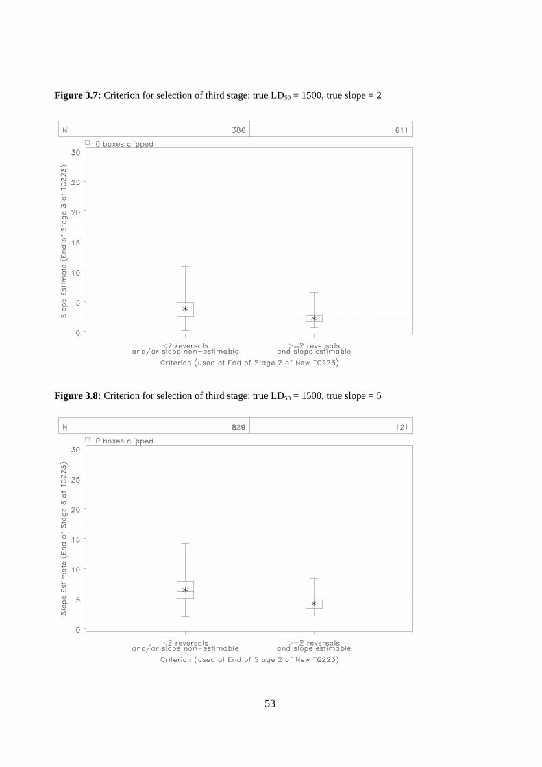
53
Figure 3.7: Criterion for selection of third stage: true LD50 = 1500, true slope = 2
Figure 3.8: Criterion for selection of third stage: true LD50 = 1500, true slope = 5

54
Figure 3.9: Criterion for selection of third stage: true LD50 = 1500, true slope = 10

55
Figure 4.1: Criterion for using fourth stage: true LD50 = 5, true slope = 2
Figure 4.2: Criterion for using fourth stage: true LD50 = 5, true slope = 5

56
Figure 4.3: Criterion for using fourth stage: true LD50 = 5, true slope = 10
Figure 4.4: Criterion for using fourth stage: true LD50 = 50, true slope = 2

57
Figure 4.5: Criterion for using fourth stage: true LD50 = 50, true slope = 5
Figure 4.6: Criterion for using fourth stage: true LD50 = 50, true slope = 10

58
Figure 4.7: Criterion for using fourth stage: true LD50 = 1500, true slope = 2
Figure 4.8: Criterion for using fourth stage: true LD50 = 1500, true slope = 5

59
Figure 4.9: Criterion for using fourth stage: true LD50 = 1500, true slope = 10
Figure 5.1: Effect of initial guess of LD50 on standard design: true LD50 = 5

60
Figure 5.2: Effect of initial guess of LD50 on standard design: true LD50 = 50
Figure 5.3: Effect of initial guess of LD50 on standard design: true LD50 = 1500

61
Figure 5.4: Effect of initial guess value of LD50 on standard design: true slope = 2
Figure 5.5: Effect of initial guess of LD50 on standard design: true slope = 5

62
Figure 5.6: Effect of initial guess of LD50 on standard design: true slope = 10
Figure 6.1: Effect of natural mortality on TG223 design: true LD50 = 5

63
Figure 6.2: Effect of natural mortality on TG223 design: true LD50 = 50
Figure 6.3: Effect of natural mortality on TG223 design: true LD50 = 1500

64
Figure 6.4: Effect of natural mortality on TG223 design: true slope = 2
Figure 6.5: Effect of natural mortality on TG2233 design: true slope = 5

65
Figure 6.6: Effect of natural mortality on TG223 design: true slope = 10
Figure 7.1: Effect of delayed mortality on TG223 design; true LD50 = 5

66
Figure 7.2: Effect of delayed mortality on TG223 design; true LD50 = 50
Figure 7.3: Effect of delayed mortality on TG223 design; true LD50 = 1500

67
Figure 7.4: Effect of delayed mortality on TG223 design; true slope = 2
Figure 7.5: Effect of delayed mortality on TG223 design; true slope = 5

68
Figure 7.6: Effect of delayed mortality on TG223 design; true slope = 10
Figure 8.1: Effect of initial guess of LD50 on TG223 design: true LD50 = 5

69
Figure 8.2: Effect of initial guess of LD50 on TG223 design: true LD50 = 50
Figure 8.3: Effect of initial guess of LD50 on TG223 design: true LD50 = 1500

70
Figure 8.4: Effect of initial guess of LD50 on TG223 design: true slope = 2
Figure 8.5: Effect of initial guess of LD50 on TG223 design: true slope = 5

71
Figure 8.6: Effect of initial guess of LD50 on TG223 design: true slope = 10

72
Appendix II – Validation of statistical simulations
Validation of Simulations for the
Draft OECD Test Guideline Avian Acute Oral Toxicity (TG223)
Author: Carol Yarrow
Date: 28th
March 2008
Summary
Computer simulations were used to assess the performance of the proposed test design for OECD Test
Guideline Avian Acute Toxicity (TG223). A validation study to independently corroborate the results of
these simulations has now been successfully completed. Despite identifying a minor issue regarding the
specification of random seeds, this validation study has confirmed that the original simulations carried out
by Roberta Dark performed as intended and that they gave a good indication of the performance of the test
under the hypothesized circumstances.
Introduction
The purpose of this report is to document the validation process for the computer simulations that were
used to assess the performance of the proposed test design for TG223. These computer simulations used
SAS programs to simulate and analyse test data. They have been fully described in the document entitled
―Description of Simulations for the Draft OECD Test Guideline Avian Acute Oral Toxicity (TG223)‖
written by Roberta Dark and dated 30th January 2008 (hereafter this document is referred to as the
‗Description document‘).
Description of Validation Process
The validation testing of the SAS programs used to simulate the proposed test design was logically
conceived as three separate steps. The three steps are described in Sections 3.1, 3.2 and
3.3 below.
3.1 Step 1
The first step of the validation process was to confirm that the SAS program analysis.sas, which classifies
and analyses dose response data, works as intended. In order to do this, the validation programmer (CSY)
wrote her own SAS code to perform the classification and analysis of dose response data as described in
Sections 3.1 and 3.2 of the Description document. The validation programmer did not view the original
analysis.sas prior to writing and testing this code.
The validation code for analysis.sas was tested by classifying and analysing the following datasets and
comparing the results with those produced by the original analysis.sas. In each case the results were
expected to be in complete agreement.
A set of forty datasets specifically developed to test this code. These were chosen to encompass
all of the design classifications (A to G). They were provided in the SAS dataset
testdata.sas7bdat and presented in Table 2.1 in Appendix 2 of the Description document. The

73
results produced by analysis.sas for these datasets were provided in the SAS dataset
ests_testdata.sas7bdat and presented in Tables 2.2 and 2.3 in Appendix 2 of the Description
document.
A set of twelve of the nine thousand simulated datasets that had been selected to test this code.
These were provided in the SAS dataset sims_stg4_12.sas7bdat and presented in Tables 3.1.1 to
3.1.12 in Appendix 3 of the Description document. This set of datasets comprised at least one
simulated dataset from each of the nine combinations of true LD50 and true slope. The results
produced by analysis.sas for these datasets were provided in the SAS dataset
ests_stg4_12.sas7bdat and presented in Tables 3.2.1 to 3.2.12 and 3.3.1 to 3.3.12 in Appendix 3
of the Description document.
The entire original set of nine thousand simulated experiments contained in the SAS datasets
sims_stg12.sas7bdat, sims_stg3.sas7bdat and sims_stg4.sas7bdat (note that this was not required
in the Description document, but it was done for completeness). The results produced by
analysis.sas for these datasets were provided in the SAS datasets ests_stg12.sas7bdat,
ests_stg3.sas7bdat and ests_stg4.sas7bdat.
3.1 Step 2
The second step of the validation process was to confirm that the SAS program results.sas, which produces
boxplots and summary tables to present the results of the simulated datasets, works as intended. In order to
do this, the validation programmer wrote her own SAS code to present the results of the original set of nine
thousand simulated datasets. These results were provided in the SAS dataset ests_stg4.sas7bdat. The
validation programmer did not view the original results.sas prior to writing and testing this code.
The results of the validation code for results.sas were then compared to the results of the original
results.sas. The results were expected to be in complete agreement.
3.1 Step 3
The third and final step of the validation process was to confirm that the SAS programs stg12.sas, stg3.sas
and stg4.sas that were used to simulate the proposed test design work as intended. In order to do this, the
validation programmer wrote her own SAS code to produce a second set of nine thousand simulated
datasets based on the descriptions in Sections 2 and 3 of the Description document. The validation
programmer did not view the original programs prior to writing and testing this code.
This new set of simulated data was then analysed using the validation code generated in Step 1 and
presented using the validation code generated in Step 2. The results were compared with the results of the
original set of simulated data that are presented in Appendix 1 of the Description document. The results
were not expected to be in complete agreement, but they were expected to be very similar.
Results of Validation Process
3.1Step 1
A SAS program, csy_analysis.sas, was developed to classify and analyse the dose response data according
to Sections 3.1 and 3.2 of the Description document.
Csy_analysis.sas was used to analyse and classify the test set of forty datasets in
testdata.sas7bdat. For each of the forty datasets the consistency, number of partials, number of

74
reversals, classification group, LD50 estimate, LD50 confidence interval, slope estimate and slope
confidence interval were checked. Results were checked both manually against the results
presented in Tables 2.2 and 2.3 in the Description document and by electronic comparison with
ests_testdata.sas7bdat using PROC COMPARE in SAS (with an equality criterion of
0.0000001). Complete agreement between the results of csy_analysis.sas and the original
analysis.sas was achieved.
Issue: Note that Table 4 in the Description document does not explicitly state that the confidence
interval for the LD50 generated using Fieller‘s theorem in the probit analysis should be a two-sided
95% confidence interval. However, this is the default in PROC PROBIT and this is what was
generated and compared by the validation programmer.
Csy_analysis.sas was used to analyse and classify the set of twelve simulated experiments that
were contained in sims_stg4_12.sas7bdat. For each of the twelve experiments the consistency,
number of partials, number of reversals, classification group, LD50 estimate, LD50 confidence
interval, slope estimate and slope confidence interval were checked after Stage 2, Stage 3 and
Stage 4 (if applicable). Results were checked both manually against the results presented in
Tables 3.2.1 to 3.2.12 and Tables 3.3.1 to 3.3.12 in the Description document and by electronic
comparison with ests_stg4_12.sas7bdat using PROC COMPARE in SAS (with an equality
criterion of 0.0000001).
For one of these experiments, (ID=7, Sim=115), there was initial disagreement between the LD50
estimate from analysis.sas (LD50_est = 3330) and csy_analysis.sas (LD50_est = non-estimable)
after Stage 2. This experiment was classified as Group F by both programs at this stage which
means that non-linear interpolation was used to estimate the LD50. The non-linear interpolation
procedure was described in Section 3.2.3 of the Description document. Investigation showed that
the discrepancy in the LD50 estimates for this experiment was due to an incomplete definition for
the case where the median response (50% mortality) was actually observed. This is the case where
m(j)/n(j) is EQUAL to 0.5, for any particular dose level x(j).
If the median response was observed, the original analysis.sas gave the LD50 estimate as the dose
at which the median response occurred. For example, for the experiment described above (ID=7,
Sim=115), 50% mortality (1 dead from 2 exposed) was observed at the highest dose of 3330. This
was the value that was given to LD50_est. The validation programmer felt that this was appropriate
and after discussion between the original programmer and the validation programmer this omission
in the description of the procedure was addressed by adding the following text to Section 3.2.3 of
the Description document (note that this was included in the version dated 30th January 2008):
“Note: If 50% mortality is observed then the estimate of the LD50 obtained using the non-
linear interpolation procedure above is simply the dose at which 50% mortality is observed.”
Csy_analysis.sas was modified according to this definition and complete agreement between the
results of csy_analysis.sas and the original analysis.sas was then achieved.
i. Csy_analysis.sas was used to analyse and classify the entire set of nine thousand simulated
experiments that were contained in sims_stg12.sas7bdat (after Stage 2), sims_stg3.sas7bdat (after
Stage 3) and sims_stg4.sas7bdat (after Stage 4). For each of the nine thousand experiments and
after each stage the consistency, number of partials, number of reversals, classification group, LD50
estimate and confidence interval and slope estimate and confidence interval were checked. Results
were checked by electronic comparison with ests_stg12.sas7bdat, ests_stg3.sas7bdat and
ests_stg4.sas7bdat using PROC COMPARE in SAS (with an equality criterion of 0.0000001).

75
Complete agreement between the results of csy_analysis.sas and the original analysis.sas was
achieved.
The SAS programs for the validation of analysis.sas are included in Appendix 2.
3.2Step 2
A SAS program, csy_results.sas, was developed to present the results of the analyses of the simulated data
as described in Section 4 of the Description document.
Csy.results.sas was used to present the results of the original set of nine thousand simulated experiments
provided in the SAS dataset ests_stg4.sas7bdat. The newly presented results were manually compared
against those presented in Appendix 1 in the Description document that had been produced by the original
results.sas. Complete agreement between the results of csy_results.sas and the original results.sas was
achieved.
The SAS programs for the validation of results.sas are included in Appendix 3.
3.3Step 3
SAS programs csy_stg12.sas, csy_stg3.sas and csy_stg4.sas were developed to produce a second set of
nine thousand simulated experiments based on the descriptions in Sections 2 and 3 of the Description
document. This data was then analysed using csy_analyse.sas and the results were presented using
csy_results.sas. These results were compared with those presented in Appendix 1 of the Description
document.
Comparison of Estimates of LD50 and Slope
Percentiles of the final LD50 estimates (on a log10 scale) and final slope estimates from the original
simulations are presented in Tables 1.1 and 1.2 respectively. Note that these are the same as Tables 1.1
and 1.2 in Appendix 1 of the Description document. Percentiles of the final LD50 estimates (on a log10
scale) and final slope estimates from the validation simulations are presented in Tables 2.1 and 2.2
respectively.
Box-and-whisker plots of the final LD50 estimates (on a log10 scale) and final slope estimates for the
original and validation simulations are presented in Figures 1.1 to 1.6 and Figures 2.1 to 2.6 in Appendix 1
respectively. Note that Figures 1.1 to 1.6 are the same as Figures 1.1 to 1.6 in Appendix 1 of the
Description document. However, they have been independently generated by the validation programmer.

76
Table 1.1: Percentiles of the final LD50 estimates (on a log10 scale) for the original simulations
ID
True Parameters No. of Final Estimates
Percentiles of estimates
LD50 Slope 25th 50th
75th
1 5 2 1000 0.6536 0.7537 0.8711
2 5 5 1000 0.6665 0.7107 0.7520
3 5 10 1000 0.6820 0.7041 0.7252
4 50 2 1000 1.6079 1.7199 1.8409
5 50 5 1000 1.6607 1.7115 1.7529
6 50 10 1000 1.6764 1.7010 1.7246
7 1500 2 1000 3.0614 3.1618 3.2780
8 1500 5 1000 3.1261 3.1750 3.2244
9 1500 10 1000 3.1541 3.1780 3.2004
Table 1.2: Percentiles of the final slope estimates for the original simulations
ID
True Parameters No. of Final Estimates
Percentiles of estimates
LD50 Slope 25th
50th
75th
1 5 2 1000 2.0524 2.7374 3.7161
2 5 5 1000 4.5727 5.8177 7.7335
3 5 10 924 8.6191 11.4315 14.0268
4 50 2 1000 2.0265 2.7471 3.7147
5 50 5 999 4.5232 5.7969 7.5050
6 50 10 927 8.6286 11.1177 14.0453
7 1500 2 1000 1.7317 2.4751 3.4170
8 1500 5 998 4.5037 5.8062 7.4932
9 1500 10 937 8.6645 11.3550 13.6303

77
Table 2.1: Percentiles of the final LD50 estimates (on a log10 scale) for the validation simulations
ID
True Parameters No. of Final Estimates
Percentiles of estimates
LD50 Slope 25th
50th
75th
1 5 2 999 0.6155 0.7092 0.8026
2 5 5 1000 0.6537 0.6993 0.7413
3 5 10 1000 0.6743 0.6985 0.7226
4 50 2 1000 1.5824 1.6993 1.8101
5 50 5 1000 1.6510 1.7004 1.7496
6 50 10 1000 1.6730 1.7000 1.7228
7 1500 2 999 3.0576 3.1541 3.2629
8 1500 5 1000 3.1364 3.1814 3.2231
9 1500 10 1000 3.1536 3.1780 3.2007
Table 2.2: Percentiles of the final slope estimates for the validation simulations
ID
True Parameters No. of Final Estimates
Percentiles of estimates
LD50 Slope 25th
50th
75th
1 5 2 999 1.9579 2.6306 3.8085
2 5 5 996 4.7340 5.9642 7.6272
3 5 10 907 8.5036 11.0611 13.2470
4 50 2 1000 1.9081 2.6275 3.6311
5 50 5 997 4.7731 6.1890 8.2340
6 50 10 897 8.3475 10.8522 13.3077
7 1500 2 999 1.8130 2.5223 3.5015
8 1500 5 992 4.4769 5.8230 7.5653
9 1500 10 884 8.6754 10.9928 13.3435
Comparison of Tables 1.1 and 2.1 shows that the distribution of the estimated LD50 from the original and
validation sets of simulated data appear to be very similar.
Comparison of Tables 1.2 and 2.2 shows that the distribution of the estimated slopes for the original and
validation sets of simulated data appear to be broadly similar. However, note that for all three values of the
true LD50, slightly fewer experiments with a true slope of 10 resulted with an estimate of the slope for the
validation simulations (907, 897, 884) than for the original simulations (924, 927, 937).
In order to investigate whether the observed difference in the number of slope estimates was real or
whether it could be explained by random variation, two further sets of simulated data, Validation2 and
Validation3, were generated by using csy_stg12.sas, csy_stg3.sas and csy_stg4.sas with different random
seeds. Table 3 shows the number of experiments that resulted in an estimate of the slope for each set of
simulations for all combinations of true LD50 and true slope. Note that (for each set) there were 1,000
simulated experiments for each combination of true LD50 and slope and that the maximum number of slope
estimates in each case is therefore 1,000.

78
Table 3: Number of final slope estimates for each set of simulated data
ID
True Parameters Number of Final Slope Estimates (out of 1000)
LD50 Slope Original Validation Validation2 Validation3
1 5 2 1000 999 999 1000
2 5 5 1000 996 996 997
3 5 10 924 907 904 884
4 50 2 1000 1000 999 1000
5 50 5 999 997 997 997
6 50 10 927 897 887 884
7 1500 2 1000 999 1000 998
8 1500 5 998 992 996 997
9 1500 10 937 884 871 881
Inspection of Table 3 shows that the number of experiments with a true slope of 10 that gave a final
estimate of the slope was consistently lower for the validation simulations than for the original simulations.
Comparison of Classification of Dose Response Data at the end of Stage 4
At the end of stages 2, 3 and 4, each experiment was classified into one of seven groups depending on the
specific characteristics of the data. These seven groups were described in Section 3.1 and Table 3 of the
Description document. Table 4 shows the percentage of experiments that were classified into each of the
seven groups at the end of Stage 4 for the original set of simulations and for each of the three sets of
validation simulations.
Inspection of Table 4 shows that at the end of Stage 4:
59.9% of experiments in the original set of simulations were classified as Group C compared to
57.8%, 57.8% and 57.4% in the three sets of validation simulations.
Slightly fewer experiments were classified as each of Groups D, E and G in the original set of
simulations than in each set of validation simulations.
o Group D: 37.7% (original) vs. 38.6%, 38.3%, 38.6% (validation)
o Group E: 1.9% (original) vs. 2.7%, 2.6%, 2.7% (validation)
o Group G: 0.5% (original) vs. 1.0%, 1.3%, 1.3% (validation)

79
o Table 4: Percentage of experiments classified as each group at the end of Stage 4
Percentage of experiments (out of 9000)
Data classification Original Validation Validation2 Validation3
A 0.0% 0.0% 0.0% 0.0%
B 0.0% 0.0% 0.0% 0.0%
C 59.9% 57.8% 57.8% 57.4%
D 37.7% 38.6% 38.3% 38.6%
E 1.9% 2.7% 2.6% 2.7%
F 0.0% 0.0% 0.0% 0.0%
G 0.5% 1.0% 1.3% 1.3%
Tables 3 and 4 provide evidence that there is a small, but real, difference between the characteristics of the
results for the original and validation sets of simulated data.
Investigation of Differences in Results of Simulated Data
A thorough investigation to identify the cause of the discrepancy in the results of the original set of
simulated data and the validation sets of simulated data was carried out by the validation programmer.
Interim results from each stage and doses tested at subsequent stages were compared. In addition, at this
point the validation programmer viewed the original stg12.sas, stg3.sas and stg4.sas and compared them to
the validation programs.
This identified that the original simulation programs had specified initial seeds for random number
generation for each stage of each experiment in a systematic manner. Five different initial seeds with a
constant difference of 9,000 between them were used for each experiment (for further explanation, see
Sections 3.3.3.1 and 3.3.3.2 below). Comprehensive experimentation showed that using seeds that are
sequential or that have a constant difference between them can result in non-independence of the random
samples generated. This has been identified as the likely cause of the discrepancy in the results. The
findings of the experimentation on seed behaviour are summarised in Appendix 5.
Random Number Generation
In order to simulate the data from each experiment, in both the original and the validation simulation
programs, SAS random number CALL routines were used to generate random numbers as described
below:
To simulate the initial guess of the LD50.
The initial guess of the LD50 for each experiment was determined by selecting a random number
from a normal distribution. In both the original and validation simulation programs, the SAS
CALL routine CALL RANNOR was used to do this.
To simulate the number of dead birds at each dose at each stage:
Stage 1: from a total of 4 exposed birds
Stage 2: from a total of 10 exposed birds

80
Stage 3: from a total of 10 exposed birds
Stage 4 (if applicable): from a total of 10 exposed birds
The number of dead birds at each dose at each stage was determined by selecting a random number
from a Binomial distribution with n=number of birds exposed and p=probability of death. In both
the original and validation simulation programs, the SAS CALL routine CALL RANBIN was used
to do this.
A note on SAS CALL routines:
SAS CALL routines can be used to generate a random sample of numbers from a specified distribution.
CALL routines require a seed variable which must be given an initial value prior to the first execution of
the CALL routine; this can be user-specified or determined by the computer clock. This initial seed does
not result directly in the selection of a random value from the specified distribution, but instead generates a
stream of random numbers, each of which is used as a seed to select a value from the distribution. The
diagram in Figure 1 below illustrates how this works.
Figure 1: Illustration of use of seeds in CALL routines
Seed specification in Original Simulations
Simulation of LD50 values
In order to generate an initial guess of the LD50, the initial value of the seed variable, seed1, for each
experiment had been specified in a systematic manner using the following SAS code:
For ID=1 to 9 and sim=1 to 1000
seed1=1000*(ID-1)+sim; (values of 1 to 9,000)
This means that the seed variable, seed1, was given an initial value of 1 for the first experiment (ID=1 and
sim=1). This initial seed of 1 generated a seed of 397204094 which was then used to select a single value
Value 2
Value 3
Value 1
Seed 4
Seed 3
Seed 2
Seed 1
Initial seed
SEED variable Random value from specified distribution

81
from the normal distribution. The next seed in the stream is 2083249653 and this could have been used to
generate the next value. However, prior to the second experiment (ID=1, sim=2) the seed variable, seed1,
was re-initialised to a value of 2. This generated a seed of 794408188 which was used to select a value
from the normal distribution for the second experiment. Prior to each subsequent experiment, the seed
variable, seed1, was re-initialised to a value between 3 and 9,000 in the same way.
Simulation of number of dead birds for each stage
Similarly, in order to generate the number of dead birds for each stage, the initial value of the seed
variable, seed2, for each stage of each experiment had been specified in a systematic manner using the
following SAS code:
For ID=1 to 9 and sim=1 to 1000:
Stage 1: seed2=9000+1000*(ID-1)+sim; (values of 9,001 to 18,000)
Stage 2: seed2=18000+1000*(ID-1)+sim;(values of 18,001 to 27,000)
Stage 3: seed2=27000+1000*(ID-1)+sim;(values of 27,001 to 36,000)
Stage 4: seed2=36000+1000*(ID-1)+sim;(values of 36,001 to 45,000)
This means that the seed variable, seed2, used to generate the number of dead birds was given a new initial
value for each stage of each experiment. The initial seeds used for the first experiment (ID=1, sim=1) were
9,001 (Stage 1), 18,001 (Stage 2), 27,001 (Stage 3) and 36,001 (Stage 4). Similarly the initial seeds used
for the second experiment were 9,002, 18,002, 27,002 and 36,002 and so on.
Investigations have indicated that the constant difference of 9,000 between the four initial seeds used to
generate the number of dead birds for each experiment will have resulted in some degree of non-
independence of the data generated at each stage. This is undesirable. The extent of correlation, however,
was shown by the analyses in 4.3.4 to have a small, but ignorable, effect on the conclusions from the
original simulations.
Seed specification in Validation Simulations
For each of the three validation sets of data, a single initial seed for the whole validation exercise was
specified using a RETAIN statement as follows.
Validation: retain seed 5674564;
Validation2: retain seed 96543854;
Validation3: retain seed 29313288l;
For each set of validation simulations, this initial seed generated a single stream of unique random seeds as
shown in Figure 1. This stream of seeds was then used to determine the initial guess of the LD50 for each
experiment and the number of dead birds at each stage in each experiment. Note that this method of
specifying a single initial seed is consistent with examples of random number generation given in SAS
Help1.
Regeneration of simulated data using original programs
In order to test the hypothesis that it is the difference in the methods of seed generation that has led to the
difference in the number of slope estimates generated in the original and validation sets of simulated data,
the original programmer modified her simulation programs to specify the seeds in a similar way to the
validation programmer. The original programmer then generated a new set of 9,000 simulated datasets
using her modified programs.

82
The percentiles of the final LD50 estimates (on a log10 scale) and final slope estimates from these
regenerated simulations are presented in Tables 5.1 and 5.2 respectively. Box-and-whisker plots of the
final LD50 estimates (on a log10 scale) and final slope estimates for the regenerated simulations are
presented in Figures 3.1 to 3.6 in Appendix 1.
Table 5.1: Percentiles of the final LD50 estimates (on a log10 scale) for the regenerated simulations
ID
True Parameters No. of Final Estimates
Percentiles of estimates
LD50 Slope 25th
50th
75th
1 5 2 1000 0.6088 0.7111 0.8143
2 5 5 1000 0.6564 0.6965 0.7415
3 5 10 1000 0.6763 0.7022 0.7234
4 50 2 999 1.5917 1.7003 1.8138
5 50 5 1000 1.6536 1.6991 1.7442
6 50 10 1000 1.6742 1.6980 1.7269
7 1500 2 999 3.0541 3.1675 3.2685
8 1500 5 1000 3.1273 3.1776 3.2205
9 1500 10 1000 3.1498 3.1748 3.1995
Table 5.2: Percentiles of the final slope estimates for the regenerated simulations
ID
True Parameters No. of Final Estimates
Percentiles of estimates
LD50 Slope 25th
50th
75th
1 5 2 1000 1.9652 2.6291 3.7804
2 5 5 999 4.6030 5.9673 7.7850
3 5 10 892 8.4920 11.1927 13.3917
4 50 2 999 1.9717 2.6838 3.7696
5 50 5 997 4.5499 5.9519 7.9676
6 50 10 879 8.5026 11.0064 13.6483
7 1500 2 999 1.8130 2.5148 3.4797
8 1500 5 998 4.6690 5.9257 7.6599
9 1500 10 898 8.6095 10.8135 13.1038
Comparison of Tables 2.1 and 5.1 and Tables 2.2 and 5.2 show that distribution of the estimated LD50 and
slope from the regenerated set of simulations and the validation set of simulations are very similar. Further
comparison of Table 5.2 with Table 3 shows that the number of regenerated experiments with a true slope
of 10 that resulted in an estimate of the slope is very similar to the corresponding number for all three sets
of validation simulations.
Table 6 shows the percentage of experiments from each set of simulations that were classified as each of
the seven classification groups at the end of Stage 4.

83
Table 6: Percentage of experiments classified as each group at the end of Stage 4
Percentage of experiments (out of 9000)
Data classification Original Validation Validation2 Validation3 Regenerated
A 0.0% 0.0% 0.0% 0.0% 0.0%
B 0.0% 0.0% 0.0% 0.0% 0.0%
C 59.9% 57.8% 57.8% 57.4% 57.8%
D 37.7% 38.6% 38.3% 38.6% 38.4%
E 1.9% 2.7% 2.6% 2.7% 2.5%
F 0.0% 0.0% 0.0% 0.0% 0.0%
G 0.5% 1.0% 1.3% 1.3% 1.3%
Inspection of Table 6 shows that the percentage of regenerated experiments that were classified as each
group at the end of Stage 4 is now very similar to the corresponding percentages for the validation
simulations.
The SAS programs for the validation of stg12.sas, stg3.sas and stg4.sas are included in Appendix 4.
Conclusions
The SAS program analysis.sas which analyses and classifies dose response data has been independently
validated; complete agreement was reached and no errors were identified.
The SAS program results.sas which presents the results of the simulated datasets has been independently
validated; complete agreement was reached and no errors were identified.
The SAS programs stg12.sas, stg3.sas and stg4.sas which simulate data for the proposed test design have
been independently validated. There were no obvious differences in the distribution of the LD50 or slope
estimates between the original and validation sets of simulations. A small discrepancy was identified in
the number of experiments with a true slope of 10 that resulted in an estimate of the slope and this has been
attributed to the way in which the seeds for random number generation were specified in the original
simulations. However, this is a minor issue and has no impact on the conclusions of the original
simulation.
References
1. SAS Institute Inc., ―Using Random-Number Functions and CALL Routines,‖ SAS 9.1 Help and
Documentation, Cary, NC: SAS Institute Inc., 2000-2004
The data analysis for this paper was generated using SAS/Base, SAS/STAT and SAS/GRAPH software,
Version 9.1 of the SAS System for Windows, Copyright [2002-2003]. SAS Institute Inc., SAS, and all
other SAS Institute Inc. product or service names are registered trademarks or trademarks of SAS Institute
Inc., Cary, NC, USA.

84
Annex I of appendix 2
Simulation results:

85
Figure 1.1
Figure 1.2

86
Figure 1.4
Figure 1.3

87
Figure 1.6
Figure 1.5

88
Figure 2.2
Figure 2.1

89
Figure 2.3
N 983 995 987 1000 1000 998 972 974 980 1000 1000 1000
Figure 2.4

90
Figure 2.5
Figure 2.6

91
Figure 3.2
Figure 3.1

92
Figure 3.3
Figure 3.4

93
Figure 3.6
Figure 3.5

94
Annex 2 of Appendix 2: Programs to validate SAS program, analysis.sas.
/* VALIDATE TESTDATA.SAS */
/* Validation program for TESTDATA - 40 test datasets */
/* Author: Carol Yarrow */
/* Date: 08/03/2008 */
libname rd "d:\2008\oecd validation\rd";
libname csy "d:\2008\oecd validation\csy";
%include "d:\2008\oecd validation\csy\programs\macros\csy_analysis.sas";
/* Classify and analyse each of the 40 datasets in TESTDATA */
options mprint;
%analysis(lib=rd, data=testdata, nexpts=40, idvar=id, where=);
/* Compare the results for 40 test datasets */
title "Comparison of classification and analysis results for all 40 test datasets";
proc compare compare=csy.results_testdata(keep=id npartials nreversals LDclass
LD50_est LD50_lcl LD50_ucl b1 b1_lcl b1_ucl) base=rd.ests_testdata(keep=id npartials nreversals LDclass
LD50_est LD50_lcl LD50_ucl b1 b1_lcl b1_ucl) criterion=0.0000001 briefsummary;
id id;
run;
/* VALIDATE 12 SIMULATIONS STAGES 1, 2, 3 AND 4.SAS */
/* Validation program for sims_stg4_12 - 12 simulated datasets */
/* Author: Carol Yarrow */
/* Date: 08/03/2008 */
libname rd "d:\2008\oecd validation\rd";
libname csy "d:\2008\oecd validation\csy";
%include "d:\2008\oecd validation\csy\programs\macros\csy_analysis.sas";
/* Create a unique experiment ID variable EXPT_ID */
data sims_stg4_12;
set rd.sims_stg4_12;
expt_id=(id-1)*1000+sim;
drop j;
run;
data ests_stg4_12;
set rd.ests_stg4_12;
expt_id=(id-1)*1000+sim;
run;
/* Classify and analyse each of the 12 datasets in SIM_stg4_12 */
options mprint;
%analysis(lib=work, data=sims_stg4_12, first=1, nexpts=1, idvar=expt_id, results=NO);
%analysis(lib=work, data=sims_stg4_12, first=1001, nexpts=1001, idvar=expt_id,
results=NO);
%analysis(lib=work, data=sims_stg4_12, first=2001, nexpts=2001, idvar=expt_id,
results=NO);
%analysis(lib=work, data=sims_stg4_12, first=3001, nexpts=3001, idvar=expt_id,
results=NO);
%analysis(lib=work, data=sims_stg4_12, first=4001, nexpts=4001, idvar=expt_id,
results=NO);
%analysis(lib=work, data=sims_stg4_12, first=5001, nexpts=5001, idvar=expt_id,
results=NO);

95
%analysis(lib=work, data=sims_stg4_12, first=6001, nexpts=6001, idvar=expt_id,
results=NO);
%analysis(lib=work, data=sims_stg4_12, first=6115, nexpts=6115, idvar=expt_id,
results=NO);
%analysis(lib=work, data=sims_stg4_12, first=6169, nexpts=6169, idvar=expt_id,
results=NO);
%analysis(lib=work, data=sims_stg4_12, first=6275, nexpts=6275, idvar=expt_id,
results=NO);
%analysis(lib=work, data=sims_stg4_12, first=7001, nexpts=7001, idvar=expt_id,
results=NO);
%analysis(lib=work, data=sims_stg4_12, first=8001, nexpts=8001, idvar=expt_id,
results=NO);
/* Combine the results */
data csy.results_sims_stg4_12;
set results_sims_stg4_12_expt1
results_sims_stg4_12_expt1001
results_sims_stg4_12_expt2001
results_sims_stg4_12_expt3001
results_sims_stg4_12_expt4001
results_sims_stg4_12_expt5001
results_sims_stg4_12_expt6001
results_sims_stg4_12_expt6115
results_sims_stg4_12_expt6169
results_sims_stg4_12_expt6275
results_sims_stg4_12_expt7001
results_sims_stg4_12_expt8001;
format LD50_est LD50_guess LD50_ucl LD50_lcl 8.2; run;
/* Compare the results */
title "Comparison of classification and analysis results for 12 simulated datasets";
title2 "After Stages 1, 2, 3 and 4";
proc compare compare=csy.results_sims_stg4_12(keep=expt_id npartials nreversals LDclass
LD50_est LD50_lcl LD50_ucl b1 b1_lcl b1_ucl)
base=ests_stg4_12(keep=expt_id npartials nreversals LDclass
LD50_est LD50_lcl LD50_ucl b1 b1_lcl b1_ucl) criterion=0.0000001 briefsummary;
id expt_id;
run;
/* VALIDATE SIMULATIONS STAGES 1, 2, 3 and 4.SAS */
/* Validation program for sims_stg4 - 9,000 simulated datasets */
/* Author: Carol Yarrow */
/* Date: 08/03/2008 */
libname rd "d:\2008\oecd validation\rd";
libname csy "d:\2008\oecd validation\csy";
%include "d:\2008\oecd validation\csy\programs\macros\csy_analysis.sas";
/* Create a unique experiment ID variable EXPT_ID */
data sims_stg4;
set rd.sims_stg4;
expt_id=(id-1)*1000+sim;
drop j;
run;
data ests_stg4;
set rd.ests_stg4;
expt_id=(id-1)*1000+sim;
run;

96
/* Classify and analyse each of the 9,000 datasets in SIM_stg4 */
proc printto log="d:\2008\oecd validation\csy\log files\log file sims_stg4.txt";
run;
%analysis(lib=work, data=sims_stg4, nexpts=9000, idvar=expt_id, where=);
proc printto;
run;
/* Compare the results */
title "Comparison of classification and analysis results for all 9,000 simulated
datasets";
title2 "After Stages 1, 2, 3 and 4";
proc compare compare=csy.results_sims_stg4(keep=expt_id npartials nreversals LDclass
LD50_est LD50_lcl LD50_ucl b1 b1_lcl b1_ucl) base=ests_stg4(keep=expt_id npartials nreversals LDclass
LD50_est LD50_lcl LD50_ucl b1 b1_lcl b1_ucl) criterion=0.0000001 briefsummary;
id expt_id;
run;
/* CSY_ANALYSIS.SAS */
/* Program to create a macro to classify and analyse multiple experiments
Input data: &lib..&data
Experiment ID of first experiment analysed = &first
Experiment ID of last experiment analysed = &nexpts
Experiment ID variable = &idvar
Use &where to restrict processing to certain doses/obs if necessary */
/* Author: Carol Yarrow Date: 08/03/2008 */
/* Create macro to classify datasets based on Table 3 */
%include "d:\2008\oecd validation\csy\programs\macros\classify.sas";
/* Create macro to analyse datasets based on Table 4 */
%include "d:\2008\oecd validation\csy\programs\macros\analyse.sas";
/* Classify and analyse each of the &nexpts datasets in &lib..&data */
%macro analysis(lib=, data=, first=1, nexpts=, idvar=, where=, results=YES);
/* Classify and analyse result from each experiment one at a time */
%do i=&first %to &nexpts;
/* Reset macro vars */
%let LD50=;
%let LD50_lowerCL=;
%let LD50_upperCL=; %let slope=;
%let slope_lowerCL=;
%let slope_upperCL=;
/* Extract data from single experiment. Round the dose to 2 decimal places. */
data &data._expt&i;
set &lib..&data;
where &idvar=&i;
rounded_dose=round(dose,0.01);
/* Recalculate logdose based on rounded dose */
logdose=log10(rounded_dose);
run;
/* Sort by rounded_dose */
proc sort data=&data._expt&i;
by rounded_dose;

97
&where;
run;
/* Combine doses (sum totals exposed, dead and alive) if rounded_dose is the same */
proc means data=&data._expt&i noprint nway;
var ndead nalive nexpo;
class rounded_dose logdose;
output out=combined_&data._expt&i sum=ndead nalive nexpo n=n;
run;
/* Calculate no. of reversals, no. of partials and classify data for each expt */
%classify(lib=&lib, data=&data._expt&i, idvar=&idvar, id=&i, print=YES, freq=NO);
/* Analyse the data for each experiment depending upon the class */
%analyse(data=&data._expt&i, idvar=&idvar, id=&i);
%end;
/* Combine results from all experiments together */
%if &results=YES %then %do;
data csy.results_&data;
set
%do j=&first %to &nexpts;
results_&data._expt&j
%end;
;
format LD50_est LD50_guess LD50_ucl LD50_lcl 8.2; run;
%end;
%mend analysis;
/* CLASSIFY.SAS */
/* Macro program to classify an experiment according to the rules in Table 3 */
/* Author: Carol Yarrow */
/* Date: 08/03/2008 */
/* Macro to classify experiment based on Table 3 */
%macro classify(lib=, data=, id=, idvar=, print=YES, freq=NO);
data classify_&data;
&idvar=&id;
set combined_&data end=last;
retain Complete_Mortality Complete_Survival NPartials
Cum_Sum_Logdose_Mortality Cum_Sum_Logdose_Survival Cum_NDead Cum_NAlive
Previous_Mortality NReversals Dose_Complete_Survival Dose_Complete_Mortality
Lower_Bound Upper_Bound AllDoses_Survival_LT_Mortality;
/* Calculate proportion of mortality and survival at each dose for each experiment */
Mortality=Ndead/Nexpo;
Survival=Nalive/Nexpo;
/* Initialise values at the beginning of each experiment */
/* Initialise Complete_Mortality and Complete_Survival to 1 if there is complete
mortality or survival at the first dose and to 0 otherwise */
/* Initialise NPartials and NReversals to 0 */
/* Initialise cumulative sums for logdose and ndead and nalive to 0 */
/* Initialise Previous_Mortality to missing at first dose as no previous dose */
/* Initialise Dose_Complete_Survival to 0 */
if _n_=1 then do;
if Mortality=1 then Complete_Mortality=1;
else Complete_Mortality=0;
if Survival=1 then Complete_Survival=1;
else Complete_Survival=0;

98
NPartials=0;
Cum_Sum_Logdose_Mortality=0;
Cum_Sum_Logdose_Survival=0;
Cum_NDead=0;
Cum_NAlive=0;
Previous_Mortality=.;
NReversals=0;
Dose_Complete_Survival=0;
Dose_Complete_Mortality=0;
Lower_Bound=" ";
Upper_Bound=" ";
AllDoses_Survival_LT_Mortality=" ";
end;
/* COMPLETE MORTALITY and COMPLETE SURVIVAL */
/* If mortality or survival at current and all subsequent doses=1 (100%) then there
is complete mortality or survival up to this dose */
if Mortality=1 and Complete_Mortality=1 then Complete_Mortality=1;
else Complete_Mortality=0;
if Survival=1 and Complete_Survival=1 then Complete_Survival=1;
else Complete_Survival=0;
/* PARTIAL MORTALITY */
/* There is partial mortality at a dose if there are both survivors and deaths */
if Mortality ne 1 and Survival ne 1 then Partial_Mortality=1;
else Partial_Mortality=0;
/* Sum the number of partial mortalities in an experiment */
NPartials + Partial_Mortality;
/* CONSISTENCY */
/* Calculate average logdose for survival and average log dose for mortality */
/* Sum logdose for mortality and survival separately for each dose */
Sum_Logdose_Mortality=Ndead*logdose;
Sum_Logdose_Survival=Nalive*logdose;
/* Calculate cumulative sums of logdose for mortality and survival for each expt */
Cum_Sum_Logdose_Mortality + Sum_Logdose_Mortality;
Cum_Sum_Logdose_Survival + Sum_Logdose_Survival;
/* Calculate cumultive sums of the number of dead and alive birds for each expt */
Cum_Ndead + Ndead;
Cum_Nalive + Nalive;
/* Calculate the average logdose for mortality and survival on the last dose for
each experiment */
if last then do;
if Cum_Ndead ne 0 then
Average_Logdose_Mortality=Cum_Sum_Logdose_Mortality/Cum_Ndead;
if Cum_Nalive ne 0 then
Average_Logdose_Survival=Cum_Sum_Logdose_Survival/Cum_Nalive;
/* If the average log dose for mortality is less than or equal to the average
Logdose for survival then the results are defined as inconsistent. Don't do this
Calculation if there is complete mortality or complete survival as one value
will be missing and it is not relevant (as the experiment will be classified as
Type A) */
if Complete_Mortality ne 1 and Complete_Survival ne 1 then do;
if Average_Logdose_Mortality<=Average_Logdose_Survival then
Consistent="Inconsistent";
else Consistent="Consistent";
end;
end;
/* REVERSALS */

99
/* Data is sorted by dose within experiment */
/* Compare mortality in each dose to mortality in the previous dose; if it is less
Then a reversal has occurred */
if previous_mortality ne . then do;
if mortality lt previous_mortality then NReversals+1;
end;
previous_mortality=mortality;
/* BOUNDS */
/* If there has been complete survival at a dose then set Dose_Complete_Survival to
1 for all subsequent doses for that experiment */
if Complete_Survival=1 then Dose_Complete_Survival=1;
/* If there is a partial mortality then if there is complete survival at a lower
dose set Lower_Bound to "Yes" */
if Partial_Mortality=1 then do;
if Dose_Complete_Survival=1 then Lower_Bound="Yes";
end;
/* If there is a partial mortality then if there is complete mortality at a higher
dose
set Upper_Bound to "Yes" */
if NPartials>=1 then do;
if Mortality=1 then Upper_Bound="Yes";
end;
/* Are all doses with complete survival below those with complete mortality? */
/* If there has been complete mortality at a dose then set Dose_Complete_Mortality
to 1 for all subsequent doses for that experiment. If there is a subsequent dose
with complete survival then the answer is No. */
if Mortality=1 then Dose_Complete_Mortality=1;
if Dose_Complete_Mortality=1 and Survival=1 then
AllDoses_Survival_LT_Mortality="No";
/* Only continue and output if the last row for each experiment */
if last;
/* Classify each experiment */
if Complete_Survival=1 or Complete_Mortality=1 then LDClass="A";
if Consistent="Inconsistent" then LDClass="B";
else if Consistent="Consistent" then do;
if NPartials>=2 then LDClass="C";
if NPartials<2 and NReversals>=1 then LDClass="D";
if NPartials=1 and NReversals=0 then do;
if Lower_Bound="Yes" and Upper_Bound="Yes" then LDClass="E";
else if Lower_Bound="Yes" or Upper_Bound="Yes" then LDClass="F";
end;
if NPartials=0 and AllDoses_Survival_LT_Mortality ne "No" then LDClass="G";
end;
keep &idvar NPartials NReversals Consistent LDClass;
run;
%mend classify;
/* ANALYSE.SAS */
/* Macro program to analyse datasets according to the rules in Table 4 */
/* Author: Carol Yarrow */
/* Date: 08/03/2008 */
%include "d:\2008\oecd validation\csy\programs\macros\probit.sas";
%include "d:\2008\oecd validation\csy\programs\macros\nonlinear.sas";
%include "d:\2008\oecd validation\csy\programs\macros\midpoint.sas";
%include "d:\2008\oecd validation\csy\programs\macros\justci.sas";
%include "d:\2008\oecd validation\csy\programs\macros\notest.sas";

100
%include "d:\2008\oecd validation\csy\programs\macros\binomial.sas";
/* Macro to analyse datasets based on classification and Table 4 */
%macro analyse(data=, idvar=, id=&i);
/* Read in class of experiment from classify result and store in macro var &CLASS */
data _null_;
set classify_&data;
call symput('class',LDClass);
run;
/* Carry out appropriate analysis for this experiment based on the classification
result */
/* If class=A then just estimate LD50 CI using Binomial_bounds */ %if &class=A %then %do;
%justci(data=&data, idvar=&idvar, id=&id);
%end;
/* If class=B then nothing estimable */
%if &class=B %then %do;
%notest(data=&data, idvar=&idvar, id=&id);
%end;
/* If class=C or D then estimate LD50, slope and CIs using probit analysis */ %if &class=C or &class=D %then %do;
%probit(data=&data, idvar=&idvar, id=&id);
%end;
/* If class=E or F then estimate LD50 using non-linear interpolation provided 50%
Mortality is bracketed, non-estimable otherwise. Estimate LD50 CI using Binomial_bounds */
%if &class=E or &class=F %then %do;
%nonlinear(data=&data, idvar=&idvar, id=&id);
%end;
/* If class=G then estimate LD50 using midpoint on log10 scale between highest dose
with complete survival and lowest dose with complete mortality Estimate LD50 CI using Binomial_bounds */
%if &class=G %then %do;
%midpoint(data=&data, idvar=&idvar, id=&id);
%end;
/* Include the estimate of LD50 and slope with the results of the classification */ data results_&data;
merge classify_&data results_&data;
by &idvar;
/* Save the guess of the LD50 in a macro var so that can replace if necessary Using rules in table 2 in order to simulate next step data */
call symput(' LD50_guess', LD50_est); run;
/* If there is no estimate of the LD50, create a working LD50 using the rules in Table 2 */
%if & LD50_guess=. %then %do; data _null_;
set combined_&data end=last;
mortality=ndead/nexpo;
retain lowdose highdose comp_mort_dose part_mort_dose LD50_guess; if _n_=1 then lowdose=rounded_dose;

101
if last then highdose=rounded_dose;
%if &class=A %then %do;
/* If complete mortality at all doses then LD50_guess = lowest dose */ if mortality=1 then LD50_guess=lowdose;
/* If complete survival at all doses then LD50_guess = highest dose */
if mortality=0 then LD50_guess=highdose; %end;
%else %if &class=B %then %do;
/* If there is a dose with complete mortality then LD50_guess = lowest dose with complete mortality */
if mortality=1 and comp_mort_dose=. then comp_mort_dose=rounded_dose;
/* If no doses with complete mortality then LD50=highest dose with partial mortality */
if 0<mortality<1 then part_mort_dose=rounded_dose;
if comp_mort_dose ne . then LD50_guess=comp_mort_dose;
else LD50_guess=part_mort_dose; %end;
%else %if &class=F %then %do;
total_ndead+ndead;
total_nexpo+nexpo;
if last then do;
if total_ndead/total_nexpo>0.5 then LD50_guess=lowdose;
else if total_ndead/total_nexpo<0.5 then LD50_guess=highdose; end;
%end;
if last;
call symput(' LD50_guess', LD50 _guess); run;
%put LD50_guess=& LD50_guess; %end;
/* Add the guess of the LD50for cases where it was missing */ data results_&data;
set results_&data;
LD50_guess= LD50_est;
if LD50_guess=. then LD50_guess=& LD50_guess; run;
%mend analyse;
/* PROBIT.SAS
Macro program to analyse datasets using probit analysis */
/* Author: Carol Yarrow */
/* Date: 08/03/2008 */
%macro probit(data=, idvar=, id=);
/* Probit analysis - Model proportion of dead birds as a function of logdose */
/* Use INVERSECL option to obtain CI for the LD50*/ ods listing close;
ods output ParameterEstimates=parameterestimates
ProbitAnalysis=probitanalysis;

102
proc probit data=combined_&data inversecl;
model ndead/nexpo=logdose;
run;
/* Extract slope estimate and CIs into macro vars */
/* Extract LD50 estimate and CIs into macro vars Need to find 10^estimate and 10^CL as doses are on the log10 scale */
data results_&data;
&idvar=&id;
set parameterestimates(keep=parameter estimate lowerCL uppercl
where=(parameter="logdose")
rename=(estimate=b1 lowerCL=b1_lcl upperCL=b1_ucl));
set probitanalysis(keep=probability variable lowerCL upperCL
where=(round(probability,0.01)=0.50)
rename=(variable=logLD50 lowerCL=log LD50_lowerCL
upperCL=logLD50_upperCL)); call symput('Slope',put(b1,8.4));
call symput('Slope_lowerCL',put(b1_lcl,8.4));
call symput('Slope_upperCL',put(b1_ucl,8.4));
LD50_est=10**log LD50;
LD50_lcl=10**log LD50_lowerCL;
LD50_ucl=10**log LD50_upperCL;
call symput('',put(LD50_est,10.2));
call symput(' LD50_lcl',put(LD50_lcl,10.2));
call symput(' LD50_ucl',put(LD50_ucl,10.2)); drop parameter probability;
run;
ods listing;
%mend probit; /* NONLINEAR.SAS
Macro program to analyse datasets using non-linear interpolation */
/* Author: Carol Yarrow */
/* Date: 08/03/2008 */
%macro nonlinear(data=, idvar=, id=);
/* Estimate LD50 using non-linear interpolation */ /* Inititalise macro vars to missing */
%let J=;
%let D=;
%let N=;
%let F=;
%let LD50_est=;
%let LD50_lcl=;
%let LD50_ucl=;
/* Non-linear interpolation */
data nonlinear;
set combined_&data;
/* Step 1: Calculate Q for each dose level (in radians) */
q_rad=1/2 * (arsin(sqrt(ndead/(nexpo+1))) + arsin(sqrt((ndead+1)/(nexpo+1))));
/* Convert Q to degrees */
q_deg=q_rad*(180/constant('PI'));
/* Calculate the mortality at each dose */
Mortality=ndead/nexpo;
run;
/* Transpose the mortality data to a single row with one column for each dose */
proc transpose data=nonlinear out=tran_mortality prefix=MORT_;
var mortality;
run;

103
/* Step 2: Find dose level j where doses j and j+1 appear to enclose the median
Dose. i.e. Mortality < 0.5 for dose j and mortality > 0.5 for dose j+1
OR dose level d where median mortality is observed */
data _null_;
set tran_mortality;
array mortality(*) _numeric_;
retain j;
do i=1 to dim(mortality);
/* If mortality=0.5 at any dose level then store the level in d */
if mortality(i)=0.5 then d=i;
if i<=dim(mortality)-1 then do;
if mortality(i)<0.5 and mortality(i+1)>0.5 then j=i;
end;
end;
/* Store the value of d in a macro variable &d */
if d ne . then call symput('D',trim(left(d)));
/* Store the value of j in a macro variable &j */
if j ne . then call symput('J',trim(left(j)));
/* Store N, the number of dose levels, in a macro variable &n */
call symput('N',trim(left(dim(mortality))));
run;
/* If the median dose was observed then this is the estimated LD50*/ %if &d ne %then %do;
/* Transpose the logdose data to give a single row with one column for each dose
level */
proc transpose data=nonlinear out=tran_logdose prefix=LOGDOSE_;
var logdose;
run;
data _null_;
set tran_logdose;
array LOGDOSE(&n) LOGDOSE_1-LOGDOSE_&n;
W=logdose(&d);
LD50_est=10**W;
/* Store the value of LD50_est in a macro variable & LD50_est */
call symput(' LD50_est', LD50_est); run;
/* Dose &d-1 is the highest dose below the estimated LD50*/
/* Dose &d+1 is the lowest dose above the estimated LD50 */
/* Find the CI for the LD50 using binomial bounds */ %binomial(data=combined_&data, id=&id);
data results_&data;
&idvar=&id;
LD50_est=&LD50_est;
%if &LD50_lcl ne %then %do;
LD50_lcl=&LD50_lcl; %end;
%if &LD50_ucl ne %then %do;
LD50_ucl=&LD50_ucl; %end;
run;
%end;
/* If the median dose is bracketed then use non-linear interpolation to find LD50*/ %else %do;

104
%if &j ne %then %do;
/* Transpose the Q function data to give a single row with one column for each
dose level */
proc transpose data=nonlinear out=tran_q prefix=Q_;
var q_deg;
run;
/* Step 3: Find the fraction, f of the interval on the angular response scale
From response q(j) to 45 degrees */
data _null_;
array Q(&n) Q_1-Q_&n;
set tran_q;
F=(45-q(&j))/(q(%eval(&j+1))-q(&j));
/* Store the value of F in a macro variable &f */
call symput('F',f);
drop _name_;
run;
%put F= &f;
/* Transpose the logdose data to give a single row with one column for each
dose level */
proc transpose data=nonlinear out=tran_logdose prefix=LOGDOSE_;
var logdose;
run;
/* Step 4: Determine the log10 dose, W, that is this fraction up from
logdose(j)and represents an estimate of the log10(LD50) */ data _null_;
set tran_logdose;
array LOGDOSE(&n) LOGDOSE_1-LOGDOSE_&n;
W=logdose(&j) + &f*(logdose(%eval(&j+1))-logdose(&j));
LD50_est=10**W;
/* Store the value of LD50_est in a macro variable &LD50_est */
call symput('LD50_est',LD50_est); run;
/* Find the CI for the LD50 using binomial bounds */ %binomial(data=combined_&data, id=&id);
data results_&data;
&idvar=&id;
LD50_est=&LD50_est;
%if &LD50_lcl ne %then %do;
LD50_lcl=&LD50
_lcl;
%end;
%if &LD50_ucl ne %then %do;
LD50_ucl=&LD50_ucl; %end;
run;
%end;
/* If the median dose is not bracketed then the LD50 is non-estimable */ %else %if &j= %then %do;
%let LD50_est=.; /* If the highest dose has less than 50% mortality then it represents the
highest dose below the 'estimated LD50' and is dose j for purposes of

105
calculating bounds */
/* If the lowest dose has more than 50% mortality then it represents the lowest
dose above the 'estimated LD50' and is dose j+1 for purposes of calculating bounds */
data _null_;
set tran_mortality;
array mortality(*) _numeric_;
if mortality(dim(mortality))<0.5 then call symput('J',dim(mortality));
if mortality(1)>0.5 then call symput('J',0);
run;
/* Find the CI for the LD50 using binomial bounds */ %binomial(data=combined_&data, id=&id);
data results_&data;
&idvar=&id;
retain LD50_est;
%if &LD50 _lcl ne %then %do;
LD50_lcl=&LD50_lcl; %end;
%if &LD50_ucl ne %then %do;
LD50_ucl=&LD50_ucl; %end;
run;
%end;
%end;
%mend nonlinear;
/* MIDPOINT.SAS */
/* Macro program to estimate LD50 using midpoint on log10 scale between highest dose with complete survival and lowest dose with complete mortality.
Used for datasets of Type G with no partial mortalities and consistent data
therefore these doses will be adjacent */
/* Author: Carol Yarrow */
/* Date: 08/03/2008 */
%macro midpoint(data=, idvar=, id=);
%let J=;
%let N=;
%let D=;
%let LD50_est=;
%let LD50_lcl=;
%let LD50_ucl=;
data midpoint;
set combined_&data;
retain previous_mortality j;
/* Calculate the mortality at each dose */
Mortality=ndead/nexpo;
/* Set j to be the highest dose level with complete survival. j+1 will be the
lowest dose level with complete mortality */
if Previous_mortality=0 and mortality=1 then j=_n_-1;
call symput('J',j);
Previous_mortality=mortality;
run;
%put j=&j;
/* Transpose the mortality data to a single row with one column for each dose level*/
proc transpose data=midpoint out=tran_logdose prefix=LOGDOSE_;

106
var logdose;
run;
/* Find the midpoint between logdose(j) and logdose(j+1) */
data _null_;
set tran_logdose;
array logdose(*) _numeric_;
/* Store N, the number of dose levels, in a macro variable &n */
call symput('N',trim(left(dim(logdose))));
logLD50=mean(logdose(&j),logdose(%eval(&j+1)));
LD50_est=10**logLD50;
/* Store the value of LD50_est in a macro variable &LD50_est */
call symput('LD50_est',LD50_est); run;
/* Find the CI for the LD50 using binomial bounds */
%binomial(data=combined_&data, id=&id);
data results_&data;
&idvar=&id;
LD50_est=&LD50_est;
%if &LD50_lcl ne %then %do;
LD50_lcl=&LD50_lcl; %end;
%if &LD50_ucl ne %then %do;
LD50_ucl=&LD50_ucl; %end;
run;
%mend midpoint;
/* JUSTCI.SAS */
/* Macro program to estimate CIs for LD50 using binomial bounds, but
missing values for LD50 and slope est and CI (dataset type A) */ /* Author: Carol Yarrow */
/* Date: 08/03/2008 */
%macro justci(data=, idvar=, id=);
/* Datasets of Type A have complete mortality or complete survival at all doses */
%let D=;
%let J=;
%let N=;
%let LD50_est=;
%let LD50_lcl=;
%let LD50_ucl=;
/* Find dose level j */
data justci;
set combined_&data;
retain j;
/* Calculate the mortality at each dose */
Mortality=ndead/nexpo;
/* If complete survival at all doses, then the highest dose is dose j, the
highest dose with complete survival */
if mortality=0 then j=_n_;
/* If complete mortality at all doses, then the lowest dose is dose j+1, the
lowest dose with complete mortality */
if mortality=1 then j=0;

107
call symput('J',j);
/* Store N, the number of dose levels, in a macro variable &n */
call symput('N',trim(left(_n_)));
run;
/* Find the CI for the LD50 using binomial bounds */ %binomial(data=combined_&data, id=&id);
data results_&data;
&idvar=&id;
retain LD50_est;
%if & LD50_lcl ne %then %do;
LD50_lcl=&LD50_lcl; %end;
%if &LD50_ucl ne %then %do;
LD50_ucl=&LD50_ucl; %end;
run;
%mend justci;
/* NOTEST.SAS */
/* Macro program to give missing values for LD50 and slope ests and CIs */ /* Author: Carol Yarrow */
/* Date: 08/03/2008 */
%macro notest(data=, idvar=, id=);
data results_&data;
&idvar=&id;
run;
%mend notest;
/* BINOMIAL.SAS
Macro program to estimate confidence limits for LD50 using Binomial confidence
bounds */
/* Author: Carol Yarrow */
/* Date: 08/03/2008 */
%macro binomial(data=, id=);
/* Estimate CI for LD50 using Binomial upper and/or lower 97.5% confidence bounds Transpose the NDEAD and NEXPO data to give a single row with one column for each
dose level */
proc transpose data=&data out=tran_ndead prefix=NDEAD_;
var ndead;
run;
proc transpose data=&data out=tran_nexpo prefix=NEXPO_;
var nexpo;
run;
proc transpose data=&data out=tran_dose prefix=DOSE_;
var rounded_dose;
run;
/* Merge the NDEAD and NEXPO data together.
Calculate the binomial cumulative distribution function for each dose level to
find:
- the probability of observing at MOST NDEAD responses from a binomial

108
dist with sample size NEXPO and prob 0.5, CB=cdf('binom',ndead,0.5,nexpo) and
- the probabiltiy of observing at LEAST NDEAD responses from a binomial dist
with sample size NEXPO and prob 0.5, RB=1-cdf('binom',ndead-1,0.5,nexpo)*/
data bounds;
array ndead(&n) NDEAD_1-NDEAD_&n;
array nexpo(&n) NEXPO_1-NEXPO_&n;
array dose(&n) DOSE_1-DOSE_&n;
array cb(&n) cb_1-cb_&n;
array rb(&n) rb_1-rb_&n;
merge tran_ndead tran_nexpo tran_dose;
do i=1 to &n;
cb(i)=cdf('binom',ndead(i),0.5,nexpo(i));
rb(i)=1-cdf('binom',ndead(i)-1,0.5,nexpo(i));
end;
/* LOWER BOUND */
/* If the median dose is observed (&d ne missing), then the highest dose below
the LD50 is &d-1. */
/* Else macro variable &j represents the highest dose level below the est LD50. Determine whether cb(&j)<=(100-97.5).
- If true then dose(&j) is lower 97.5% bound for the LD50*/
%if &d ne %then %do;
if &d-1>0 then do;
if cb(&d-1)<=(1-0.975) then LD50_lcl=dose(&d-1);
/* - If false then determine whether cb(&d-1)*cb(&d-2)<=(100-97.5).
- If true then dose(&d-2) is lower 97.5% bound for the LD50. Continue stepping down through doses and multiplying until lower bound is
found or there are no more dose levels and &d-1-k=0 */
else do;
l=cb(&d-1);
do k=1 to &n;
if &d-1-k>=1 and LD50_lcl=. then do; l=l*cb(&d-1-k);
if l<=(1-0.975) then LD50_lcl=dose(&d-1-k); end;
end;
end;
end;
%end;
%else %if &j ne %then %do;
if &j>0 then do;
if cb(&j)<=(1-0.975) then LD50_lcl=dose(&j); /* - If false then determine whether cb(&j)*cb(&j-1)<=(100-97.5).
- If true then dose(&j-1) is lower 97.5% bound for the LD50. Continue stepping down through doses and multiplying until lower bound is
found or there are no more dose levels and &j-k=0 */
else do;
l=cb(&j);
do k=1 to &n;
if &j-k>=1 and LD50_lcl=. then do;
l=l*cb(&j-k);
if l<=(1-0.975) then LD50_lcl=dose(&j-k); end;
end;
end;

109
end;
%end;
/* Store the value of LD50_lcl in a macro variable & LD50_lcl */
call symput(' LD50_lcl', LD50 _lcl);
/* UPPER BOUND */
/* Macro variable &j+1 represents the lowest dose level above the estimated LD50. Determine whether rb(&j+1)<=(100-97.5).
If true then dose(&j+1) is upper 97.5% bound for the LD50*/
%if &d ne %then %do;
if &d+1<=&n then do;
if rb(&d+1)<=(1-0.975) then LD50_ucl=dose(&d+1);
/* If false then determine whether rb(&d+1)*rb(&d+2)<=(100-97.5).
If true then dose(&d+2) is upper 97.5% bound for the LD50. Continue stepping up through doses and multiplying until upper bound is
found or there are no more dose levels and &d+1+k>&n */
else do;
u=rb(&d+1);
do k=1 to &n;
if &d+1+k<=&n and LD50_ucl=. then do; u=u*rb(&d+1+k);
if u<=(1-0.975) then LD50_ucl=dose(&d+1+k); end;
end;
end;
end;
%end;
%else %do;
if &j+1<=&n then do;
if rb(&j+1)<=(1-0.975) then LD50_ucl=dose(&j+1);
/* If false then determine whether rb(&j+1)*rb(&j+2)<=(100-97.5).
If true then dose(&j+2) is upper 97.5% bound for the LD50. Continue stepping up through doses and multiplying until upper bound is
found or there are no more dose levels and &j+1+k>&n */
else do;
u=rb(&j+1);
do k=1 to &n;
if &j+1+k<=&n and LD50_ucl=. then do; u=u*rb(&j+1+k);
if u<=(1-0.975) then LD50_ucl=dose(&j+1+k); end;
end;
end;
end;
%end;
/* Store the value of LD50_ucl in a macro variable & LD50_ucl */
call symput(' LD50_ucl', LD50_ucl); run;
%mend binomial;

110
Annex 3 of appendix 2: Programs to validate SAS program, results.sas.
/* VALIDATE RESULTS.SAS */
/* Program to validate presentation of the results of the simulations according to
Section 4 */
/* Input data: RD.ESTS_STG4
/* Author: Carol Yarrow */
/* Date: 08/03/2008 */
%include "d:\2008\oecd validation\csy\programs\macros\csy_results.sas";
data ests_stg4;
set rd.ests_stg4;
log_ LD50 =log10(LD50_est);
label log_ LD50="log LD50 Estimate" slope="True slope"
b1="Slope Estimate"
LD50="True LD50"; run;
%results(data=ests_stg4, title="Presentation of results of ESTS_STG4");
/* CSY_RESULTS.SAS */
/* Program to create macro to present the results of the simulations according to
Section 4 */
/* Author: Carol Yarrow */
/* Date: 08/03/2008 */
%macro results(data=&data, title="Presentation of results from ESTS_STG4",
outdata="d:\temp\results.csv");
/* Produce boxplot of results */
%macro boxplot(data=, var=, group=, LD50=, slope=, where=, vaxis=, vformat=4.1, title=, title2=);
goptions reset=all;
goptions fontres=presentation ftext=duplex htext=1.3;
symbol v=star h=1.5;
%if & LD50 ne %then %let vref=%sysfunc(log10(&LD50)); %if &slope ne %then %let vref=&slope;
proc boxplot data=&data;
title &title;
title2 &title2;
plot &var*&group / vref=&vref &vaxis vformat=&vformat
clipfactor=1.5 cliplegend='# Boxes clipped' clipsubchar = '#'
cliplegpos=top clipsymbol=square;
insetgroup n / position=topoff;
&where;
run;
%mend boxplot;
options mprint;
%boxplot(data=&data, var=log_LD50, group=slope, LD50=5, where=where LD50=& LD50, title=&title, vaxis=vaxis=(-0.5 to 1.5 by 0.5), title2="Box and whisker
plot of LD50 estimates where true LD50=& LD50 ");
%boxplot(data=&data, var=log_ LD50, group=slope, LD50=50, where=where LD50=&LD50, title=&title, vaxis=vaxis=(0.5 to 3.0 by 0.5), title2="Box and whisker
plot of LD50 estimates where true LD50=& LD50");

111
%boxplot(data=&data, var=log_LD50, group=slope, LD50=1500, where=where LD50=&LD50, title=&title, vaxis=vaxis=(2.0 to 4.0 by 0.5), title2="Box and whisker
plot of LD50 estimates where true LD50=&LD50");
%boxplot(data=&data, var=b1, group=LD50, slope=2, where=where slope=&slope, title=&title, vaxis=vaxis=(0 to 30 by 5), vformat=2., title2="Box and
whisker plot of slope estimates where true slope=&slope");
%boxplot(data=&data, var=b1, group=LD50, slope=5, where=where slope=&slope, title=&title, vaxis=vaxis=(0 to 30 by 5), vformat=2., title2="Box and
whisker plot of slope estimates where true slope=&slope");
%boxplot(data=&data, var=b1, group=LD50, slope=10, where=where slope=&slope, title=&title, vaxis=vaxis=(0 to 30 by 5), vformat=2., title2="Box and
whisker plot of slope estimates where true slope=&slope" );
/* Print out percentiles of final LD50 and slope estimates */ proc means data=&data nway noprint;
var LD50_est b1;
class LD50 slope; output out=percentiles n= p25= p50= p75= / autoname;
run;
/* Find the percentiles of LD50 on the log10 scale */
data percentiles;
set percentiles;
log_LD50_p25=log10(LD50_est_p25);
log_LD50_p50=log10(LD50_est_p50);
log_LD50_p75=log10(LD50_est_p75); run;
title &title;
title2 "Percentiles of the final LD50 estimates on a log 10 scale"; proc print data=percentiles label noobs;
var LD50 slope LD50_est_n log_LD50_p25 log_LD50_p50 log_LD50_p75;
format log_LD50_p25 log_LD50_p50 log_LD50_p75 8.4;
label LD50_n="No. of Final Estimates"
log_LD50_p25="25th percentile"
log_LD50_p50="50th percentile"
log_LD50_p75="75th percentile"; run;
title2 "Percentiles of the final slope estimates";
proc print data=percentiles label;
var LD50 slope b1_n b1_p25 b1_p50 b1_p75; format b1_p25 b1_p50 b1_p75 8.4;
label b1_n="No. of Final Estimates"
b1_p25="25th percentile"
b1_p50="50th percentile"
b1_p75="75th percentile";
run;
proc export data=percentiles outfile=&outdata dbms=csv replace;
run;
%mend results;

112
Annex 4 of appendix 2: Programs to validate SAS programs, stg12.sas, stg3.sas and stg4.sas.
/* RUN SIMULATIONS.SAS */
/* Program to simulate dose response data according to Section 2.1 and 2.2
Output dataset CSY.CSY_STG4 and CSY.RESULTS.CSY_STG4 */
/* Author: Carol Yarrow */
/* Date: 08/03/2008 */
libname rd "d:\2008\oecd validation\rd";
libname csy "d:\2008\oecd validation\csy";
%include "d:\2008\oecd validation\csy\programs\csy_stg12.sas";
%include "d:\2008\oecd validation\csy\programs\csy_stg3.sas";
%include "d:\2008\oecd validation\csy\programs\csy_stg4.sas";
/* Present results of simulations */
%include "d:\2008\oecd validation\csy\programs\macros\csy_results.sas";
options mprint;
%results(data=csy.results_csy_stg4, title="Presentation of results of CSY_STG4");
/* CSY_STG12.SAS */
/* Program to simulate dose response data according to Section 2.1 and 2.2
Output dataset CSY.CSY_STG12 and CSY.RESULTS_CSY_STG12 */
/* Author: Carol Yarrow */
/* Date: 08/03/2008 */
options mprint;
%include "d:\2008\oecd validation\csy\programs\macros\dose.sas";
%include "d:\2008\oecd validation\csy\programs\macros\mortality.sas";
%include "d:\2008\oecd validation\csy\programs\macros\csy_analysis.sas";
%global seed;
/* STAGE 1*/
/* Generate a computer simulated guess of the LD50 using random number from normal
distribution with mean equal to true log10(LD50) and variance consistent with the
95th and 5th percentile being a factor of 10 greater or less than the true LD50.
This corresponds to the 5th percentile of logLD50 being 1 less than the true
logLD50. As the 5th percentile of the normal distribution is 1.6449 SDs less than the true mean, this corresponds to using a SD of 1/1.6449 */
/* Generate initial guess of LD50 for each of 9,000 experiments */ title;
data csy.LD50; retain seed 5674564;
do Expt_id=1 to 9000;
/* Select random number from the standard normal distribution */
call rannor(seed,x);
/* Define true LD50 and true slope values for each experiment */
/* True LD50=5 for expts 1-3000, =50 for expts 3001-6001 and
=1500 for expts 6001-9000 */
if 1<=Expt_id<=3000 then LD50=5;
if 3001<=Expt_ID<=6000 then LD50=50;

113
if 6001<=Expt_ID<=9000 then LD50=1500;
/* True slope=2 for expts 1-1000, 3001-4000 and 6001-7000 */
/* True slope=5 for expts 1001-2000, 4001-5000 and 7001-8000 */
/* True slope=10 for expts 2001-3000, 5001-6000 and 8001-9000 */
if 1<=Expt_ID<=1000 or 3001<=Expt_ID<=4000 or 6001<=Expt_ID<=7000 then slope=2;
if 1001<=Expt_ID<=2000 or 4001<=Expt_ID<=5000 or 7001<=Expt_ID<=8000 then
slope=5;
if 2001<=Expt_ID<=3000 or 5001<=Expt_ID<=6000 or 8001<=Expt_ID<=9000 then
slope=10;
/* Create mu as the log10 of the true LD50*/
mu=log10(LD50);
/* Use the random number from normal dist to generate random number from normal
distribution with mean log10(LD50) and standard deviation of 1/1.6449 */
log LD50_guess=mu+(1/1.6449)*x;
LD50_guess=10**log LD50_guess; Slope_guess=.;
/* Save the last value of SEED in a macro variable to use as starting seed
for next sequence of random numbers */
call symput('seed',seed);
output;
end;
drop x mu logLD50_guess; run;
/* Run PROC MEANS to verify that the 5th percentile and 95th percentile of the
estimated LD50s from each distribution (for each different value of mu) are a factor of 10 greater or less than the true value. Verified. */
title "Confirmation that the 5th and 95th percentiles are a factor of 10 greater or
less than true mu";
proc means data=csy. LD50 p5 median p95;
var LD50_guess;
class LD50 run;
%let lowlim=1;
%let upplim=3330;
/* Generate doses for Stage 1 */
data stage1_doses;
set csy. LD50;
dose1= LD50_guess/sqrt(50);
dose4= LD50_guess*sqrt(50); if dose1<&lowlim then do;
dose1=&lowlim;
dose4=dose1*50;
end;
if dose4>&upplim then do;
dose4=&upplim;
dose1=dose4/50;
end;
dose2=dose1*50**(1/3);
dose3=dose1*50**(2/3);
nexpo=1;
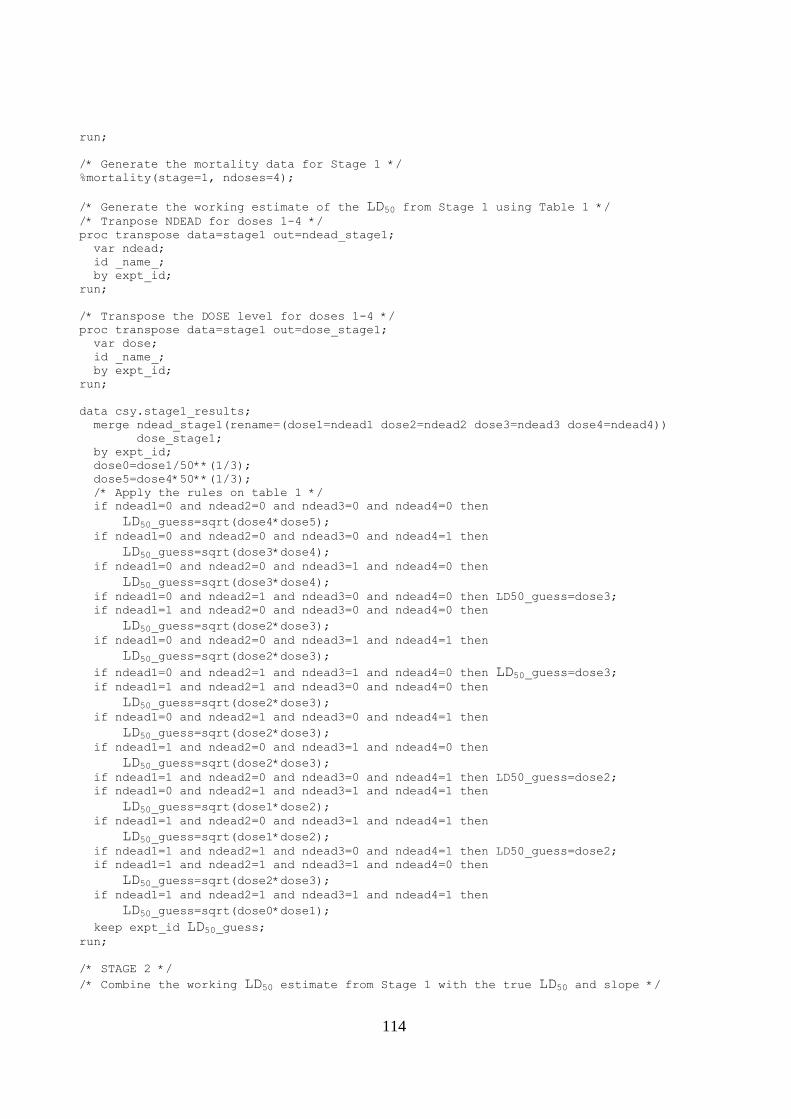
114
run;
/* Generate the mortality data for Stage 1 */
%mortality(stage=1, ndoses=4);
/* Generate the working estimate of the LD50 from Stage 1 using Table 1 */ /* Tranpose NDEAD for doses 1-4 */
proc transpose data=stage1 out=ndead_stage1;
var ndead;
id _name_;
by expt_id;
run;
/* Transpose the DOSE level for doses 1-4 */
proc transpose data=stage1 out=dose_stage1;
var dose;
id _name_;
by expt_id;
run;
data csy.stage1_results;
merge ndead_stage1(rename=(dose1=ndead1 dose2=ndead2 dose3=ndead3 dose4=ndead4))
dose_stage1;
by expt_id;
dose0=dose1/50**(1/3);
dose5=dose4*50**(1/3);
/* Apply the rules on table 1 */
if ndead1=0 and ndead2=0 and ndead3=0 and ndead4=0 then
LD50_guess=sqrt(dose4*dose5); if ndead1=0 and ndead2=0 and ndead3=0 and ndead4=1 then
LD50_guess=sqrt(dose3*dose4); if ndead1=0 and ndead2=0 and ndead3=1 and ndead4=0 then
LD50_guess=sqrt(dose3*dose4); if ndead1=0 and ndead2=1 and ndead3=0 and ndead4=0 then LD50_guess=dose3;
if ndead1=1 and ndead2=0 and ndead3=0 and ndead4=0 then
LD50_guess=sqrt(dose2*dose3); if ndead1=0 and ndead2=0 and ndead3=1 and ndead4=1 then
LD50_guess=sqrt(dose2*dose3);
if ndead1=0 and ndead2=1 and ndead3=1 and ndead4=0 then LD50_guess=dose3; if ndead1=1 and ndead2=1 and ndead3=0 and ndead4=0 then
LD50_guess=sqrt(dose2*dose3); if ndead1=0 and ndead2=1 and ndead3=0 and ndead4=1 then
LD50_guess=sqrt(dose2*dose3); if ndead1=1 and ndead2=0 and ndead3=1 and ndead4=0 then
LD50_guess=sqrt(dose2*dose3); if ndead1=1 and ndead2=0 and ndead3=0 and ndead4=1 then LD50_guess=dose2;
if ndead1=0 and ndead2=1 and ndead3=1 and ndead4=1 then
LD50_guess=sqrt(dose1*dose2); if ndead1=1 and ndead2=0 and ndead3=1 and ndead4=1 then
LD50_guess=sqrt(dose1*dose2); if ndead1=1 and ndead2=1 and ndead3=0 and ndead4=1 then LD50_guess=dose2;
if ndead1=1 and ndead2=1 and ndead3=1 and ndead4=0 then
LD50_guess=sqrt(dose2*dose3); if ndead1=1 and ndead2=1 and ndead3=1 and ndead4=1 then
LD50_guess=sqrt(dose0*dose1);
keep expt_id LD50_guess; run;
/* STAGE 2 */
/* Combine the working LD50 estimate from Stage 1 with the true LD50 and slope */

115
/* Calculate the doses for Stage 2 */
data stage2_doses;
merge csy.stage1_results csy. LD50 (drop=LD50_guess slope_guess); array dose(10);
by expt_id;
/* Calculate lowdose and highdose */
%dose(lowprob=0.01, highprob=0.99, LD50_guess= LD50_guess, slope_guess=5); do i=1 to 10;
dose(i)=lowdose*r**((i-1)/9);
end;
nexpo=1;
drop i;
run;
/* Generate the mortality data for Stage 2 */
%mortality(stage=2, ndoses=10);
/* Concatenate the data from Stages 1 and 2 together */
data csy.csy_stg12;
set stage1 stage2;
by expt_id;
run;
/* Analyse the data from Stages 1 and 2 together */
options nomprint;
proc printto log="d:\2008\oecd validation\csy\log files\log file csy_stg12.txt";
run;
%analysis(lib=csy, data=csy_stg12, nexpts=9000, idvar=expt_id, where=);
proc printto;
run;
/* CSY_STG3.SAS */
/* Program to simulate dose response data according to Section 2.1 and 2.2
Input dataset CSY.CSY_STG12 and CSY.RESULTS_CSY_STG12
Output dataset CSY.CSY_STG3 and CSY.RESULTS_CSY_STG3 */
/* Author: Carol Yarrow */
/* Date: 08/03/2008 */
%include "d:\2008\oecd validation\csy\programs\macros\dose.sas";
%include "d:\2008\oecd validation\csy\programs\macros\mortality.sas";
%include "d:\2008\oecd validation\csy\programs\macros\csy_analysis.sas";
/* STAGE 3*/
/* Combine the working LD50 and slope estimates from Stage 2 with the true LD50 and slope */
options mprint;
data stage3_doses;
merge csy.results_csy_stg12(keep=expt_id nreversals LD50_guess b1 rename=(b1=slope_guess))
csy. LD50 (drop= LD50_guess slope_guess); by expt_id;
array dose(5);
/* Calculate the doses for Stage 3 */
/* If the working estimate of the slope is greater than 15 or less than one it is
Set to these bounds */
if slope_guess<1 and slope_guess ne . then slope_guess=1;
if slope_guess>15 then slope_guess=15;
/* If at the end of Stage 2 there are 2 or more reversals and a working estimate of
The slope has been obtained, stage 3a is used. Otherwise Stage 3b is used */

116
/* Stage 3a */
if nreversals>=2 and slope_guess ne . then do;
/* Calculate lowdose and highdose */
%dose(lowprob=0.15, highprob=0.85, LD50_guess= LD50_guess, slope_guess=slope_guess);
dose1=lowdose;
dose2=highdose;
nexpo=5;
end;
/* Stage 3b */
else do;
/* Calculate lowdose and highdose */
%dose(lowprob=0.15, highprob=0.85, LD50_guess= LD50_guess, slope_guess=5); do i=1 to 5;
dose(i)=lowdose*r**((i-1)/4);
end;
nexpo=2;
end;
run;
/* Generate the mortality data for Stage 3 */
options mprint;
%mortality(stage=3, ndoses=5);
/* Concatenate the data from Stages 1, 2 and 3 together */
data csy.csy_stg3;
set csy.csy_stg12 stage3;
by expt_id;
run;
/* Analyse the data from Stages 1 and 2 together */
proc printto log="d:\2008\oecd validation\csy\log files\log file csy_stg3.txt";
run;
%analysis(lib=csy, data=csy_stg3, nexpts=9000, idvar=expt_id, where=);
proc printto; run; /* CSY_STG4.SAS */
/* Program to simulate dose response data according to Section 2.1 and 2.2
Input dataset CSY.CSY_STG3 and CSY.RESULTS_CSY_STG3
Output dataset CSY.CSY_STG4 and CSY.RESULTS_CSY_STG4 */
/* Author: Carol Yarrow */
/* Date: 08/03/2008 */
%include "d:\2008\oecd validation\csy\programs\macros\dose.sas";
%include "d:\2008\oecd validation\csy\programs\macros\mortality.sas";
%include "d:\2008\oecd validation\csy\programs\macros\csy_analysis.sas";
/* STAGE 4*/
/* If there are two or more reversals and/or twwo or more partial kills at the end of
Stage 3 then the experiment stops. Otherwise the experiment continues to stage 4*/
/* Combine the working LD50 and slope estimates from Stage 3 with the true LD50 and slope */
data stage4_doses;
merge csy.results_csy_stg3(keep=expt_id nreversals npartials LD50_guess b1 rename=(b1=slope_guess))
csy. LD50 (drop= LD50_guess slope_guess); by expt_id;
array dose(5);
/* If the working estimate of the slope is greater than 15 or less than one it is
set to these bounds */

117
if slope_guess<1 and slope_guess ne . then slope_guess=1;
if slope_guess>15 then slope_guess=15;
/* If at the end of Stage 3 there are 2 or more reversals and/or two or more
Partial kills and a working estimate of the slope then the experiment stops.
Else continues to Stage 4 */
if (nreversals>=2 or npartials>=2) and slope_guess ne . then delete;
/* Calculate the doses for Stage 4 */
else do;
/* Calculate lowdose and highdose */
%dose(lowprob=0.15, highprob=0.85, LD50_guess= LD50_guess, slope_guess=5); do i=1 to 5;
dose(i)=lowdose*r**((i-1)/4);
end;
nexpo=2;
end;
run;
/* Generate the mortality data for Stage 4 */
options mprint;
%mortality(stage=4, ndoses=5);
/* Concatenate the data from Stages 1, 2, 3 and 4 together */
data csy.csy_stg4;
set csy.csy_stg3 stage4;
by expt_id;
run;
/* Analyse the data from Stages 1, 2, 3 and 4 together */
options nomprint;
proc printto log="d:\2008\oecd validation\csy\log files\log file csy_stg4.txt";
run;
%analysis(lib=csy, data=csy_stg4, nexpts=9000, idvar=expt_id, where=);
proc printto;
run;
/* DOSE.SAS */
/* Macro program to calculate lowdose and highdose based ib LD50_guess and Slope_guess*/
/* Author: Carol Yarrow */
/* Date: 08/03/2008 */
%macro dose(lowlim=1, upplim=3330, lowprob=0.01, highprob=0.99, LD50_guess= LD50_guess, slope_guess=slope_guess);
lowdose=10**(probit(&lowprob)/&Slope_guess+log10(&LD50_guess));
highdose=10**(probit(&highprob)/&Slope_guess+log10(&LD50_guess)); /* Calculate the low dose to high dose ratio */
r=highdose/lowdose;
if lowdose<&lowlim then do;
lowdose=&lowlim;
highdose=lowdose*r;
end;
if highdose>&upplim then do;
highdose=&upplim;
lowdose=highdose/r;
end;
%mend dose;

118
/* MORTALITY.SAS */
/* Macro program to calculate mortality at each stage */
/* Author: Carol Yarrow */
/* Date: 08/03/2008 */
%macro mortality(stage=1, ndoses=4);
proc transpose data=stage&stage._doses out=tran_stage&stage._doses(rename=(col1=Dose));
var dose1-dose&ndoses;
by expt_id LD50 slope nexpo; run;
/* Generate the mortality data for each dose */
data stage&stage;
Stage=&stage;
set tran_stage&stage._doses;
if dose=. then delete;
/* Use the current value of the macro variable SEED to initialise seed for
random number generation */
retain seed &seed;
logdose=log10(dose);
logLD50=log10(LD50);
/* Model the probability of death at each dose using the probit model */
if index(_NAME_,'dose')>0 then do;
probit=(-logLD50*slope) + (slope*logdose); p=probnorm(probit);
/* Generate the number dead at each dose using Binomial random number */
if p=1 then ndead=nexpo;
if p=0 then ndead=0;
if p<1 and p>0 then call ranbin(seed,nexpo,p,ndead);
nalive=nexpo-ndead;
end;
/* Save the last value of SEED in a macro variable to use as starting seed
for next sequence of random numbers */
call symput('seed',seed);
run;
%mend mortality;

119
Annex 5 of appendix 2: Summary of investigation into seed behaviour in SAS
Consequences of using systematic seeds
The advantage of specifying seeds in a systematic manner for each experiment in a simulation study is that
it is easy to regenerate the data for any particular experiment as the seeds for each experiment are known.
However, detailed investigation has shown that the use of these systematic seeds appears to introduce a
‗non-random‘ element into the samples generated.
In order to illustrate this, 100 samples of 1,000 values were generated from a binomial distribution with
n=10 and p=0.5 using:
a) Seeds generated in a systematic manner.
i.e. for i=1 to 100 and j=1 to 1000:
seed = 1000*(i-1) + j; (1 to 1000, 1001 to 2000, 2001 to 3000 etc.)
b) Seeds generated by specifying a single initial seed
retain seed 76807689;
As the data is binomially distributed, the expected variance within each of the 100 samples is np(1-p).
n*p*(1-p) = 10*0.5*0.5
= 2.5.
Figure 4 shows the estimated within-sample variance for each of the 100 samples generated by each
method. The horizontal line shows the expected value of 2.5.

120
Figure 4: Sample variances for 100 samples generated using a) systematic seeds and b) a single seed
For data generated by using both method a), systematic seeds, and method b), a single initial seed,
the observed variance of each sample was centred round the expected value of 2.5.
However, note that the spread of the within-sample variances of samples generated using
systematic seeds is far less than that for samples generated using a single initial seed. In other
words, the within-sample variances of those samples generated using systematic seeds is close to
the expected value for each sample.
In order to determine which of these methods was producing data that behaved as we would expect, the
variance of the sample means for each method was compared to its theoretical value. The expected
variance of the sample means is np(1-p)/m where m is the number of values in each sample (in each case
m=1000).
n*p*(1-p)/1000 = 2.5/1000
= 0.0025.
For data generated using systematic seeds the observed variance of the sample means was
0.0000390. This is much less (64 times less) than the expected value of 0.0025.
For data generated using a single initial seed the observed variance of the sample means was
0.00265. This is very close to the expected value of 0.0025.
The between-sample variation of data generated using systematic seeds in this example is therefore far less
than we would expect if it were truly random. Further investigation identified that the causes of this
problem are as follows:
There is a cyclic relationship between the value of the initial seed and the value of the subsequent
seed (see Figure 5 below).

121
There is a direct relationship between the value of the seed used to select NDEAD from the
binomial distribution and the value of NDEAD itself (see Figure 6 below).

122
Figure 5: Relationship between initial and subsequent values of SEED
Figure 6: Relationship between value of SEED and value of NDEAD

123
Appendix III – Evaluation of clarity of the guideline through written quizzes.
A. TG223 Avian Acute Oral Toxicity Test - Reading Comprehension Exam without answers (March
2008)
B. TG223 Avian Acute Oral Toxicity Test - Reading Comprehension Exam with correct answers
(March 2008)
C. TG223 Avian Acute Oral Toxicity Test - Results from First Quiz to Evaluate Guideline
Clarity (based on March 2007 draft, summary prepared September 2007)
D. TG223 Avian Acute Oral Toxicity Test - Results from Second Quiz to Evaluate Guideline Clarity
(based on March 2008 draft, summary prepared September 2009)

124
A. TG223 Avian Acute Oral Toxicity Test - Reading Comprehension Exam without answers
(March 2008)
1. Assume a 0 represents survival and a 1 represents a kill. For each of the following sequences,
identify the number of reversals. The sequences are listed to represent increasing dose (from left to
right) and only one bird was tested at each dose.
0001011111 _____
0011101111 _____
0101000001 _____
0001010101 _____
2. If you conduct a limit test and one bird dosed at the limit dies, what is the next step?
3. If you conduct a limit test and a control bird dies, what is the next step?
4. Compute the working estimate of the LD50 based on the following Stage 1 results.
a.
Dose 56.56 208.37 766.80 2828.4
Result * 0 0 1 0
* 0 = survival, 1=death
b.
Dose 26.9 99.0 364.6 1343.3
Result * 0 1 1 1
* 0 = survival, 1=death
5. For the following scenarios, identify the correct sequence of doses for stage 2.
a. Working estimate of LD50 = 425
i.
145.6 184.7 234.3 297.3 377.3 478.7 607.3 770.6 977.7 1240.6
ii.
145.6 215.3 318.3 470.7 696.0 1029.3 1522.1 2250.8 3328.3 4921.8
iii.
162.7 206.4 261.9 332.3 421.6 535.0 678.8 861.3 1092.8 1386.5
b. Limit test with 5 birds at 2000mg/kg, 3 mortalities at limit dose
i.
391.8 496.9 630.3 799.5 1014.1 1286.4 1631.7 2069.7 2625.3 3330.0
ii.
610.3 774.4 982.6 1246.7 1581.8 2007.0 2546.5 3231.1 4099.6 5201.7
iii.
379.8 481.9 611.5 775.9 984.4 1249.0 1584.8 2010.8 2551.3 3237.2

125
6. For each of the following scenarios, identify which option shows the correct dose sequence for
stage 3, where 0 = survival, 1=death.
a. Stage 1
Dose 7.1 26.0 96.0 353.5
Result 0 0 1 0
Stage 2
Dose 63.1 80.0 101.6 128.9 163.5 207.5 263.2 334.0 423.8 537.7
Result 0 0 0 0 0 1 1 1 1 1
i. 5 birds at 82.7 and 5 birds at 412.1
ii. 5 birds at 114.6 and 5 birds at 297.5
iii. 2 birds at each of the following doses:
114.5, 145.4, 184.6, 234.3, and 297.4
b. Limit test at 2000 mg/kg – observe 1 mortality out of 5 birds, signs of toxicity in 2 other
birds.
Stage 2
Dose 391.8 496.9 630.3 799.5 1014.1 1286.4 1631.7 2069.7 2625.3 3330.0
Result 0 0 0 0 0 0 0 1 1 1
i. 2 birds at each of the following doses:
1246.0, 1581.7, 2007.8, 2548.8, 3235.5
ii. 5 birds at 1282.5 and 5 birds at 3330
iii. 2 birds at each of the following doses:
1234.8, 1567.5, 1989.8, 2525.9, 3206.5
7. What is the next step for the following scenario?
a. Conduct limit test at 2000 mg/kg – observe 1 mortality out of 5 birds
b. Then conduct second limit test at 2000 mg/kg – observe no additional mortalities, no signs
of toxicity in any birds.
8. Under what conditions is stage 4 necessary?
9. Determine the number of partials and reversals for each of the following scenarios. The sequences
are listed in increasing dose from left to right.
(this question was not in the quiz based on the 2007 draft guideline)
a. Partials _____ Reversals ______
Number of
mortalities 0 0 0 1 0 1 2 1 1
Number of
tested
individuals
1 1 1 2 1 1 2 1 1
b. Partials _____ Reversals ______

126
Number of
mortalities 0 0 1 3 0 1 1 4 1
Number of
tested
individuals
1 1 1 5 1 1 1 5 1

127
TG223 Avian Acute Oral Toxicity Test - Reading Comprehension Exam with correct answers
(March 2008)
Assume a 0 represents survival and a 1 represents a kill. For each of the following sequences, identify
the number of reversals. The sequences are listed to represent increasing dose (from left to right) and
only one bird was tested at each dose.
0001011111 _____ 1
0011101111 _____ 1
0101000001 _____ 2
0001010101 _____ 3
1. If you conduct a limit test and one bird dosed at the limit dies, what is the next step?
if no signs of tox in other birds, dose 5 more birds at limit
If signs of tox in other birds, go to stage 2
2. If you conduct a limit test and a control bird dies, what is the next step?
If mortality could possibly be due to husbandry, need to redo test. If mortality could be considered
incidental background (not related to conduct of test), random mortality – then add an additional 5 control
birds.
3. Compute the working estimate of the LD50 based on the following Stage 1 results.
a.
Dose 56.56 208.37 766.80 2828.4
Result * 0 0 1 0
* 0 = survival, 1=death
1472.7
b.
Dose 26.9 99.0 364.6 1343.3
Result * 0 1 1 1
* 0 = survival, 1=death
51.6

128
4. For the following scenarios, identify the correct sequence of doses for stage 2.
a. Working estimate of LD50 = 425
i. correct
145.6 184.7 234.3 297.3 377.3 478.7 607.3 770.6 977.7 1240.6
ii. LD50=425 step = 50^(1/10), Max/min value for hdose removed
145.6 215.3 318.3 470.7 696.0 1029.3 1522.1 2250.8 3328.3 4921.8
iii. correct step, LD50 = 475
162.7 206.4 261.9 332.3 421.6 535.0 678.8 861.3 1092.8 1386.5
b. Limit test with 5 birds at 2000mg/kg, 3 mortalities at limit dose
i. Correct
391.8 496.9 630.3 799.5 1014.1 1286.4 1631.7 2069.7 2625.3 3330.0
ii. Max value for hdose removed
610.3 774.4 982.6 1246.7 1581.8 2007.0 2546.5 3231.1 4099.6 5201.7
iii. Used working estimate of LD50=1109
379.8 481.9 611.5 775.9 984.4 1249.0 1584.8 2010.8 2551.3 3237.2

129
5. For each of the following scenarios, identify which option shows the correct dose sequence for
stage 3, where 0 = survival, 1=death.
a. Stage 1
Dose 7.1 26.0 96.0 353.5
Result 0 0 1 0
Working LD50=184.2
Stage 2
Dose 63.1 80.0 101.6 128.9 163.5 207.5 263.2 334.0 423.8 537.7
Result 0 0 0 0 0 1 1 1 1 1
Working LD50 = 184.6
Working slope= 2.97
i. 5 birds at 82.7 and 5 birds at 412.1 correct
ii. 5 birds at 114.6 and 5 birds at 297.5 assume slope=5
iii. 2 birds at each of the following doses: correct for 3b stage
114.5, 145.4, 184.6, 234.3, and 297.4
b. Limit test at 2000 mg/kg – observe 1 mortality out of 5 birds, signs of toxicity in 2 other
birds.
Working LD50=2947
Stage 2
Dose 391.8 496.9 630.3 799.5 1014.1 1286.4 1631.7 2069.7 2625.3 3330.0
Result 0 0 0 0 0 0 0 1 1 1
Working LD50 = 1990
Working slope= not available (only one partial kill)
i. 2 birds at each of the following doses:
1246.0, 1581.7, 2007.8, 2548.8, 3235.5 stage 3b, calc done with 4
mortalities at 2000 mg/kg
ii. 5 birds at 1282.5 and 5 birds at 3330 stage 3a, assume slope=5
iii. 2 birds at each of the following doses: correct
1234.8, 1567.5, 1989.8, 2525.9, 3206.5
6. What is the next step for the following scenario?
a. Conduct limit test at 2000 mg/kg – observe 1 mortality out of 5 birds
b. Then conduct second limit test at 2000 mg/kg – observe no additional mortalities, no signs
of toxicity in any birds.
Conclude that LD50 > limit dose with 0.95 probability, no more testing required.
7. Under what conditions is stage 4 necessary?
If an estimate of the slope cannot be obtained at the conclusion of stage 3b. One needs to have two or
more reversals or partial kills to estimate slope.
8. Determine the number of partials and reversals for each of the following scenarios. The sequences
are listed in increasing dose from left to right.

130
a. Partials __1___ Reversals ___1___
Number of
mortalities 0 0 0 1 0 1 2 1 1
Number of
tested
individuals
1 1 1 2 1 1 2 1 1
b. Partials _2____ Reversals __3____
Number of
mortalities 0 0 1 3 0 1 1 4 1
Number of
tested
individuals
1 1 1 5 1 1 1 5 1

131
C. TG223 Avian Acute Oral Toxicity Test - Results from First Quiz to Evaluate Guideline
Clarity (based on March 2007 draft, summary prepared September 2007)
Responses:
2 answered correctly
for sequence (3):
one person listed 1 reversal
one person listed 3 reversals
Issues to address:
Provide examples in guideline.
Responses:
2 answered correctly
2 other answers were:
a) test 5 more at limit
b) if no signs of tox, dose 5 birds at limit, and if tox signs in remaining 4 birds then go to
stage 2.
Issues to address:
Ensure guidance is clear and consistent
1. Assume a 0 represents survival and a 1 represents a kill. For each of the
following sequences, identify the number of reversals. The sequences are listed
to represent increasing dose (from left to right) and only one bird was tested at
each dose.
0001011111 _____ 1
0011101111 _____ 1
0101000001 _____ 2
0001010101 _____ 3
2. You conduct a limit test and one bird dosed at the limit dies, what is the next
step?
If no signs of toxicity in other dosed birds, dose 5 more birds at limit
If signs of toxicity in other dosed birds, go to stage 2

132
Responses:
all four respondents answered correctly
Issues to address:
None.
Responses:
All four respondents answered correctly
Issues to address:
None
3. If you conduct a limit test and a control bird dies, what is the next step?
If mortality could possibly be due to husbandry, need to redo test. If mortality could be
considered incidental background (not related to conduct of test), random mortality – then
add an additional 5 control birds.
4. Compute the working estimate of the LD50 based on the following Stage 1 results.
a.
Dose 56.56 208.37 766.80 2828.4
Result * 0 0 1 0
* 0 = survival, 1=death
1472.7
b.
Dose 26.9 99.0 364.6 1343.3
Result * 0 1 1 1
* 0 = survival, 1=death
51.6

133
Responses:
All four respondents answered correctly
Issues to address:
None
Responses:
1 answered correctly
3 chose (ii), where maximum dose was not limited to 3330mg/kg
Issues to address:
Ensure guidance is clear.
5. For the following scenarios, identify the correct sequence of doses for stage 2.
a. Working estimate of LD50 = 425
i. correct
145.6 184.7 234.3 297.3 377.3 478.7 607.3 770.6 977.7 1240.6
ii. LD50=425 step = 50^(1/10), Max/min value for hdose removed
145.6 215.3 318.3 470.7 696.0 1029.3 1522.1 2250.8 3328.3 4921.8
iii. correct step, LD50 = 475
162.7 206.4 261.9 332.3 421.6 535.0 678.8 861.3 1092.8 1386.5
5. For the following scenarios, identify the correct sequence of doses for stage 2.
b. Limit test with 5 birds at 2000mg/kg, 3 mortalities at limit dose
i. Correct
391.8 496.9 630.3 799.5 1014.1 1286.4 1631.7 2069.7 2625.3 3330.0
ii. Max value for hdose removed
610.3 774.4 982.6 1246.7 1581.8 2007.0 2546.5 3231.1 4099.6 5201.7
iii. Used working estimate of LD50=1109
379.8 481.9 611.5 775.9 984.4 1249.0 1584.8 2010.8 2551.3 3237.2
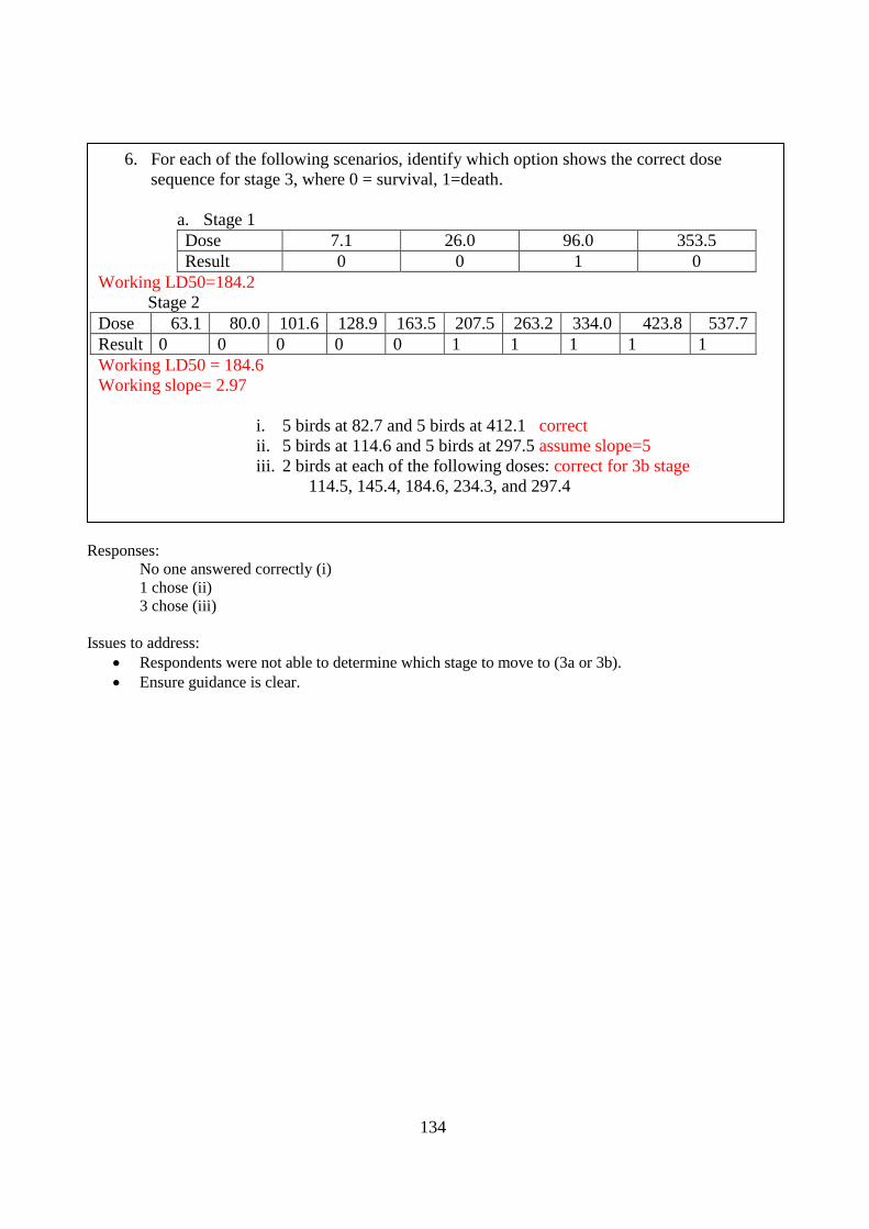
134
Responses:
No one answered correctly (i)
1 chose (ii)
3 chose (iii)
Issues to address:
Respondents were not able to determine which stage to move to (3a or 3b).
Ensure guidance is clear.
6. For each of the following scenarios, identify which option shows the correct dose
sequence for stage 3, where 0 = survival, 1=death.
a. Stage 1
Dose 7.1 26.0 96.0 353.5
Result 0 0 1 0
Working LD50=184.2
Stage 2
Dose 63.1 80.0 101.6 128.9 163.5 207.5 263.2 334.0 423.8 537.7
Result 0 0 0 0 0 1 1 1 1 1
Working LD50 = 184.6
Working slope= 2.97
i. 5 birds at 82.7 and 5 birds at 412.1 correct
ii. 5 birds at 114.6 and 5 birds at 297.5 assume slope=5
iii. 2 birds at each of the following doses: correct for 3b stage
114.5, 145.4, 184.6, 234.3, and 297.4

135
Responses:
2 chose (i)
2 stated answer was either (i) or (iii)
Issues to address:
Ensure guidance is clear.
6. For each of the following scenarios, identify which option shows the correct dose
sequence for stage 3, where 0 = survival, 1=death.
b. Limit test at 2000 mg/kg – observe 1 mortality out of 5 birds, signs of toxicity
in 2 other birds.
Working LD50=2947
Stage 2
Dose 391.8 496.9 630.3 799.5 1014.1 1286.4 1631.7 2069.7 2625.3 3330.0
Result 0 0 0 0 0 0 0 1 1 1
Working LD50 = 1990
Working slope= not available (only one partial kill)
i. 2 birds at each of the following doses:
1246.0, 1581.7, 2007.8, 2548.8, 3235.5 stage 3b, calc done with
4 mortalities at 2000 mg/kg
ii. 5 birds at 1282.5 and 5 birds at 3330 stage 3a, assume slope=5
iii. 2 birds at each of the following doses: correct
1234.8, 1567.5, 1989.8, 2525.9, 3206.5

136
Responses:
all four respondents answered correctly
Issues to address:
none
Responses:
all four respondents answered correctly
Issues to address:
None.
7. What is the next step for the following scenario?
a. Conduct limit test at 2000 mg/kg – observe 1 mortality out of 5 birds
b. Then conduct second limit test at 2000 mg/kg – observe no additional
mortalities, no signs of toxicity in any birds.
Conclude that LD50 > limit dose with 0.95 probability, no more testing required.
8. Under what conditions is stage 4 necessary?
If an estimate of the slope cannot be obtained at the conclusion of stage 3b. One
needs to have two or more reversals or partial kills to estimate slope.

137
D. TG223 Avian Acute Oral Toxicity Test - Results from Second Quiz to Evaluate Guideline
Clarity (based on March 2008 draft, summary prepared September 2009)
Responses:
All 13 respondents answered correctly.
Issues to address:
None.
Responses:
10 answered correctly
3 provided partially correct answers, those answers were:
a) either conduct another limit test or go to stage 2
b) dose an additional 5 birds at limit
c) If treatment related, add 5 more birds; or go to stage 1 or stage 2.
Issues to address:
Ensure guidance is clear.
One respondent noted concerns that one death (out of 10 birds) at the limit dose would have
harmonization issues with OPPTS 850.2100 (does not allow any deaths at limit dose). Need to
ensure that there are no concerns with harmonization. Respondent also noted concerns regarding
inferences from 5 birds dosed at limit; even with no mortalities, cannot meet required standard for
EPA endangered species assessments.
1. Assume a 0 represents survival and a 1 represents a kill. For each of the
following sequences, identify the number of reversals. The sequences are listed
to represent increasing dose (from left to right) and only one bird was tested at
each dose.
0001011111 _____ 1
0011101111 _____ 1
0101000001 _____ 2
0001010101 _____ 3
2. You conduct a limit test and one bird dosed at the limit dies, what is the next
step?
If no signs of toxicity in other dosed birds, dose 5 more birds at limit
If signs of toxicity in other dosed birds, go to stage 2

138
1 respondent stated could not find answer in guideline
4 provided partial/incorrect answers, those answers were: Responses:
8 answered correctly
a) restart expt with 5 new control birds
b) cause of death should be determined
c) five additional control birds should be added
d) repeat with 5 additional control birds
Issues to address:
Ensure guidance is clear and consistent.
Steps regarding controls needs to be in a more prominent/logical place in the guidance.
Responses:
All 13 respondents answered correctly
Issues to address:
None
5. Compute the working estimate of the LD50 based on the following Stage 1 results.
a.
Dose 56.56 208.37 766.80 2828.4
Result * 0 0 1 0
* 0 = survival, 1=death
1472.7
b.
Dose 26.9 99.0 364.6 1343.3
Result * 0 1 1 1
* 0 = survival, 1=death
51.6
4. If you conduct a limit test and a control bird dies, what is the next step?
If mortality could possibly be due to husbandry, need to redo test. If mortality could
be considered incidental background (not related to conduct of test), random
mortality – then add an additional 5 control birds.

139
Responses:
All 13 respondents answered correctly
Issues to address:
None
Responses:
9 answered correctly
4 chose (ii), where maximum dose was not limited to 3330mg/kg
Issues to address:
Ensure guidance is clear.
6. For the following scenarios, identify the correct sequence of doses for stage 2.
c. Working estimate of LD50 = 425
i. correct
145.6 184.7 234.3 297.3 377.3 478.7 607.3 770.6 977.7 1240.6
ii. LD50=425 step = 50^(1/10), Max/min value for hdose removed
145.6 215.3 318.3 470.7 696.0 1029.3 1522.1 2250.8 3328.3 4921.8
iii. correct step, LD50 = 475
162.7 206.4 261.9 332.3 421.6 535.0 678.8 861.3 1092.8 1386.5
6. For the following scenarios, identify the correct sequence of doses for stage 2.
d. Limit test with 5 birds at 2000mg/kg, 3 mortalities at limit dose
i. Correct
391.8 496.9 630.3 799.5 1014.1 1286.4 1631.7 2069.7 2625.3 3330.0
ii. Max value for hdose removed
610.3 774.4 982.6 1246.7 1581.8 2007.0 2546.5 3231.1 4099.6 5201.7
iii. Used working estimate of LD50=1109
379.8 481.9 611.5 775.9 984.4 1249.0 1584.8 2010.8 2551.3 3237.2

140
Responses:
1 answered correctly (i)
2 chose (ii)
8 chose (iii)
1 did not answer
Issues to address:
Most common error appears that Stage 1 and Stage 2 results were not combined to correctly
determine partials/reversals (there are two reversals in the example). If reader only looks at Stage 2
data, there are no reversals and the next stage would be Stage 3b (answer iii).
Staff in EFED noted difficulty calculating slope as the standard software used for LD50 calculation
(Toxanal) does not perform probit calculations for data with <2 partial mortalities. Additional
clarification will be added in guidance.
Ensure guidance is clear.
7. For each of the following scenarios, identify which option shows the correct dose
sequence for stage 3, where 0 = survival, 1=death.
a. Stage 1
Dose 7.1 26.0 96.0 353.5
Result 0 0 1 0
Working LD50=184.2
Stage 2
Dose 63.1 80.0 101.6 128.9 163.5 207.5 263.2 334.0 423.8 537.7
Result 0 0 0 0 0 1 1 1 1 1
Working LD50 = 184.6
Working slope= 2.97
i. 5 birds at 82.7 and 5 birds at 412.1 correct
ii. 5 birds at 114.6 and 5 birds at 297.5 assume slope=5
iii. 2 birds at each of the following doses: correct for 3b stage
114.5, 145.4, 184.6, 234.3, and 297.4

141
Responses:
3 answered correctly (iii)
4 chose (i)
3 stated answer was either (i) or (iii)
1 chose (ii)
1 stated answer was ‗none of the above‘
1 did not answer
Issues to address:
Most respondents were able to correctly determine that Stage 3b should be used. EFED staff noted
difficulty calculating LD50 and slope as the standard software used in EFED for LD50 calculation
(Toxanal) does not perform probit calculations for data with <2 partial mortalities.
Some staff were looking for exact calculations for the working LD50 in the guidance text; this is
not included for Stage 3 dose setting. Will clarify for next guideline draft revision.
Ensure guidance is clear.
7. For each of the following scenarios, identify which option shows the correct dose
sequence for stage 3, where 0 = survival, 1=death.
b. Limit test at 2000 mg/kg – observe 1 mortality out of 5 birds, signs of toxicity
in 2 other birds.
Working LD50=2947
Stage 2
Dose 391.8 496.9 630.3 799.5 1014.1 1286.4 1631.7 2069.7 2625.3 3330.0
Result 0 0 0 0 0 0 0 1 1 1
Working LD50 = 1990
Working slope= not available (only one partial kill)
j. 2 birds at each of the following doses:
1246.0, 1581.7, 2007.8, 2548.8, 3235.5 stage 3b, calc done with
4 mortalities at 2000 mg/kg
ii. 5 birds at 1282.5 and 5 birds at 3330 stage 3a, assume slope=5
iv. 2 birds at each of the following doses: correct
1234.8, 1567.5, 1989.8, 2525.9, 3206.5

142
Responses:
12 answered correctly
1 responded to go to Stage 2
Issues to address:
Ensure guidance is clear.
Responses:
12 answered correctly
1 responded ―if slope not defined or confidence intervals too wide‖
Issues to address:
Ensure guidance is clear.
7. What is the next step for the following scenario?
c. Conduct limit test at 2000 mg/kg – observe 1 mortality out of 5 birds
d. Then conduct second limit test at 2000 mg/kg – observe no additional
mortalities, no signs of toxicity in any birds.
Conclude that LD50 > limit dose with 0.95 probability, no more testing required.
8. Under what conditions is stage 4 necessary?
If an estimate of the slope cannot be obtained at the conclusion of stage 3b. One
needs to have two or more reversals or partial kills to estimate slope.

143
Note the following question was added after the first reading comprehension results were interpreted
and resulting changes made to guideline.
Responses:
All 13 answered the number of partials correctly for both a. and b.
Reversals for part a)
9 correct
1 responded ‗zero reversals‘
2 responded ‗two reversals‘
Reversals for part b)
3 answered correctly
other answers were 1, 2, or 6 reversals
Issues to address:
Ensure guidance is clear. Provide more clear examples.
9. Determine the number of partials and reversals for each of the following scenarios.
The sequences are listed in increasing dose from left to right.
a. Partials __1___ Reversals ___1___
Number of
mortalities 0 0 0 1 0 1 2 1 1
Number of
tested
individuals
1 1 1 2 1 1 2 1 1
b. Partials _2____ Reversals __3____
Number of
mortalities 0 0 1 3 0 1 1 4 1
Number of
tested
individuals
1 1 1 5 1 1 1 5 1
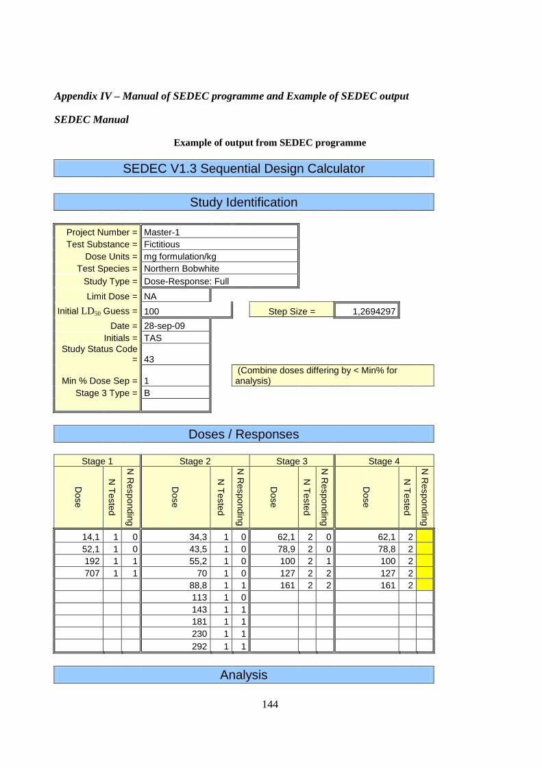
144
Appendix IV – Manual of SEDEC programme and Example of SEDEC output
SEDEC Manual
Example of output from SEDEC programme
SEDEC V1.3 Sequential Design Calculator
Study Identification
Project Number = Master-1
Test Substance = Fictitious
Dose Units = mg formulation/kg
Test Species = Northern Bobwhite
Study Type = Dose-Response: Full
Limit Dose = NA
Initial LD50 Guess = 100 Step Size = 1,2694297
Date = 28-sep-09
Initials = TAS
Study Status Code = 43
Min % Dose Sep = 1 (Combine doses differing by < Min% for analysis)
Stage 3 Type = B
Doses / Responses
Stage 1 Stage 2 Stage 3 Stage 4 D
ose
N T
este
d
N R
espo
ndin
g
Dose
N T
este
d
N R
espo
ndin
g
Dose
N T
este
d
N R
espo
ndin
g
Dose
N T
este
d
N R
espo
ndin
g
14,1 1 0 34,3 1 0 62,1 2 0 62,1 2
52,1 1 0 43,5 1 0 78,9 2 0 78,8 2
192 1 1 55,2 1 0 100 2 1 100 2
707 1 1 70 1 0 127 2 2 127 2
88,8 1 1 161 2 2 161 2
113 1 0
143 1 1
181 1 1
230 1 1
292 1 1
Analysis

145
Probit Analysis Results
Itterations Chi-square Probability G N
8 6,087097931 0,992581075 0,710195894 24
Slope = 11,89865035
95% Confidence Limits= 1,871286328 and 21,92601438
LD50 = 100,0872194
95% Confidence Limits= 71,5067982 and 139,9416652
n of Reversals = 2 n of Partials = 1
Combined Data in Dose Order
Dose Num
ber
Exp
osed
Num
ber
Dea
d
Revers
al or
Part
ial
?
% R
espo
ndin
g
Merg
ed D
oses?
14,1 1 0 - 0 -
34,3 1 0 - 0 -
43,5 1 0 - 0 -
52,1 1 0 - 0 -
55,2 1 0 - 0 -
62,1 2 0 - 0 -
70 1 0 - 0 -
78,9 2 0 - 0 -
88,8 1 1 - 100 -
100 2 1 Rev+Partial 50 -
113 1 0 Reversal 0 -
127 2 2 - 100 -
143 1 1 - 100 -
161 2 2 - 100 -
181 1 1 - 100 -
192 1 1 - 100 -
230 1 1 - 100 -
292 1 1 - 100 -
707 1 1 - 100 -

146
Dose Nu
mb
er
Exp
ose
d
Nu
mb
er
De
ad
Re
ve
rsa
l o
r
Pa
rtia
l ?
Me
rge
d D
ose
s?
14.1 1 0 - 0 -
34.3 1 0 - 0 -
43.5 1 0 - 0 -
52.1 1 0 - 0 -
55.2 1 0 - 0 -
62.1 2 0 - 0 -
70 1 0 - 0 -
78.9 2 0 - 0 -
88.8 1 1 - 100 -
100 2 1 Rev+Partial 50 -
113 1 0 Reversal 0 -
127 2 2 - 100 -
143 1 1 - 100 -
161 2 2 - 100 -
181 1 1 - 100 -
192 1 1 - 100 -
230 1 1 - 100 -
292 1 1 - 100 -
707 1 1 - 100 -
Combined Data in Dose Order
% R
esp
on
din
g