Embed Size (px)
Citation preview
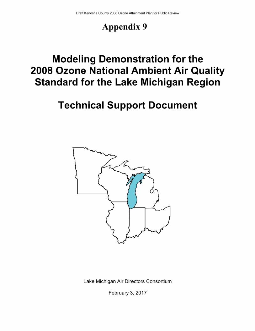
Modeling Demonstration for the 2008 Ozone National Ambient Air Quality Standard for the Lake Michigan Region
Technical Support Document
Lake Michigan Air Directors Consortium
February 3, 2017
Appendix 9
Draft Kenosha County 2008 Ozone Attainment Plan for Public Review
i
Table of Contents List of Figures ............................................................................................................. ii List of Tables ............................................................................................................... v Executive Summary .................................................................................................... 1 1.0 Introduction ........................................................................................................... 3 SIP Requirements .............................................................................................. 4 Technical Work: Overview .................................................................................. 5 2.0 Ambient Data Analyses ........................................................................................ 7 Current Conditions ... ………………………………………………………………….7 Meteorology and Transport................................................................................. 7 Ozone Air Quality Trends ......................................................... ………………..13 Conceptual Model for Ozone in the Lake Michigan Region ................................... 18 3.0 Emissions Inventory Development .................................................................... 19 U.S. EPA’s Modeling Platform .......................................................................... 19 On-Road Motor Vehicles .................................................................................. 20 Electric Generating Units .................................................................................. 21 Control Measures ............................................................................................. 25 Emissions Summary ......................................................................................... 28 4.0 Air Quality Modeling ........................................................................................... 29 Selection of Base Year …………………………………………………………..….29 Modeling Platform ............................................................................................. 29 Meteorological Inputs ....................................................................................... 31 Photochemical Model Configuration ................................................................. 32 Summary of Model Performance Evaluation .................................................... 33 Modeled Attainment Test .................................................................................. 39 Weight of Evidence Support for Attainment ...................................................... 42 5.0 Conclusions ......................................................................................................... 46 References ................................................................................................................. 48 Appendix A – Model Performance Evaluation ........................................................ 50
Draft Kenosha County 2008 Ozone Attainment Plan for Public Review
ii
List of Figures Figure 1.1. Nonattainment Areas in the Lake Michigan Region for the 2008 Ozone
National Ambient Air Quality Standard ..................................................................... 4 Figure 2.1. 8-hour Ozone Design Values (2013-2015) in the LADCO Region ............. 9 Figure 2.2. 8-hour Ozone Design Values in the Lake Michigan Region
(2014-2016) …………………..…. ............................................................................. 9 Figure 2.3. Trends in 90-degree Days and 8-hour “Exceedance” Days Around Lake
Michigan ................................................................................................................ 10 Figure 2.4. Examples of Elevated Regional Ozone Concentrations
(June 9-11, 2016) ................................................................................................... 11 Figure 2.5. Examples of High Ozone Days in the Lake Michigan Area ...................... 11 Figure 2.6. Aircraft Ozone Measurements over Lake Michigan and Along Upwind Boundary – August 20, 2003 ..................................................................... 12 Figure 2.7. Incremental Probability of Air Mass Location in 72 Hours
Prior to High Ozone Concentrations at Wisconsin Shoreline Monitors……………………………………………………………………………………13
Figure 2.8. Ozone Design Value Trends in the Chicago and Sheboygan
Nonattainment Areas ............................................................................................. 14 Figure 2.9. Trend in Fourth-High Values in the Chicago and Sheboygan
Nonattainment Areas ............................................................................................. 14 Figure 2.10. Change in Ozone Design Values from 2009-2011 to 2014-2016 ............ 15 Figure 2.11. Deviation from Long Term Average Temperature, June-August
for 2005-2016 ........................................................................................................ 16 Figure 2.12. Meteorologically Adjusted Ozone Trends Around Lake Michigan .......... 17 Figure 3.1. Vehicle Population Per Capita Used in the 2011 NEIv2 ........................... 21 Figure 3.2. Base Year (2011) and Future Year (2017) VOC and NOX Emissions
for On-Road Mobile Sources ................................................................................. 22 Figure 3.3. VOC Emissions by MOVES Rate Source................................................. 22
Draft Kenosha County 2008 Ozone Attainment Plan for Public Review
iii
List of Figures (continued)
Figure 3.4. Separation of VOC and NOx Emissions by MOVES Vehicle Group ........ 23 Figure 3.5. 2015 EIA Annual Energy Outlook – National Forecast of Power Generation for Coal and Natural Gas ................................................ …………..….25 Figure 3.6 Base Year (2011) and Future Year (2017) VOC and NOx Emissions ...... 28 Figure 4.1. Map of WRF Model Domain ................................. ………………….……..31 Figure 4.2. Photochemical Modeling Domain ........... ……………………………………33 Figure 4.3. 2011 Mean Observed MDA8 Ozone with a 60 ppb
Ozone Threshold ................................................................................................... 35 Figure 4.4. 2011 Mean CAMx Predicted MDA8 Ozone with a
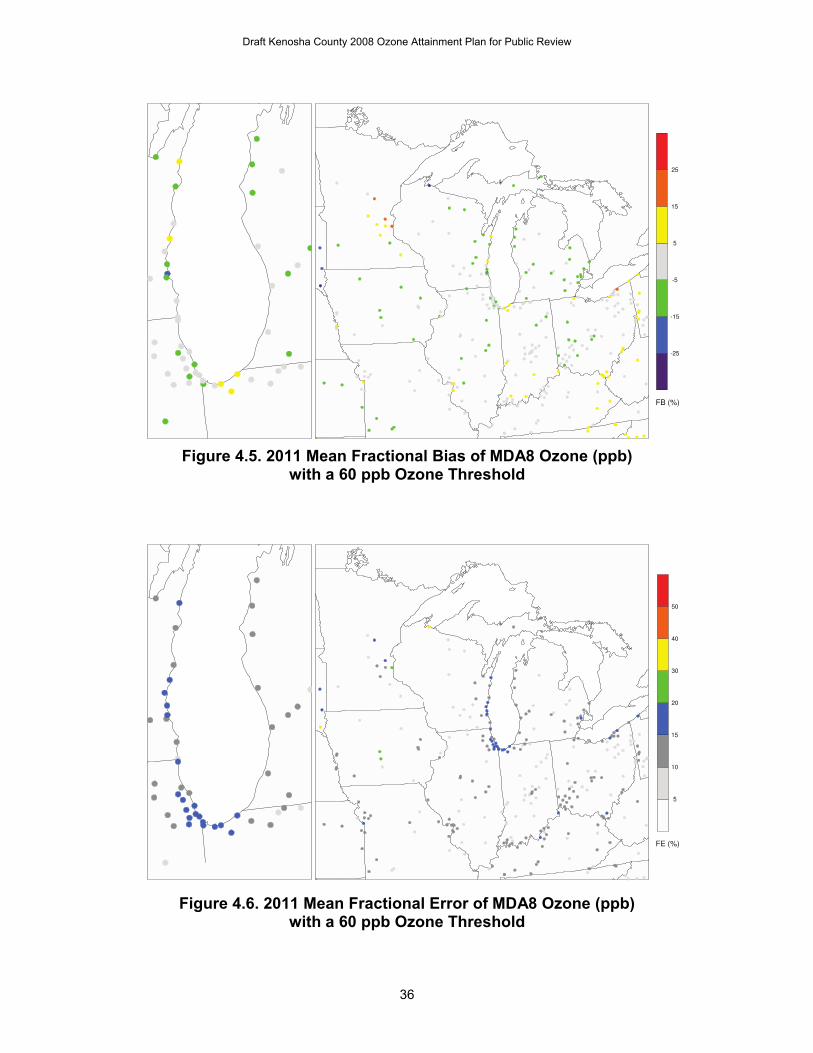
60 ppb Ozone Threshold .......................................................................................................... 35 Figure 4.5. 2011 Mean Fractional Bias of MDA8 Ozone with a
60 ppb Ozone Threshold ....................................................................................... 36 Figure 4.6. 2011 Mean Fractional Error of MDA8 Ozone with a
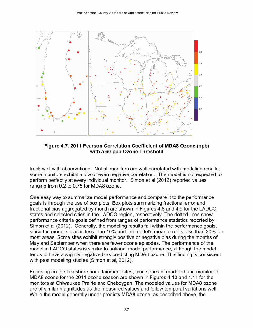
60 ppb Ozone Threshold ....................................................................................... 36 Figure 4.7. 2011 Pearson Correlation Coefficient of MDA8 Ozone
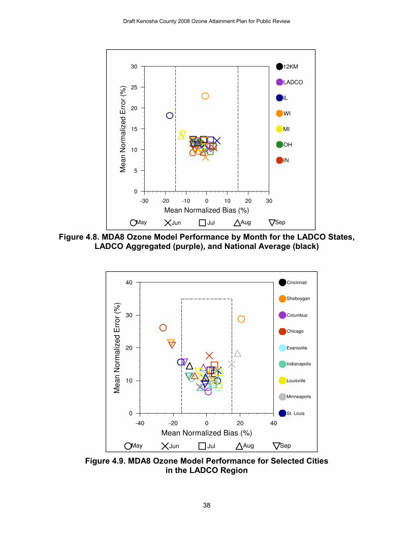
with a 60 ppb Ozone Threshold ............................................................................. 37 Figure 4.8. MDA8 Ozone Model Performance by Month for the LADCO States, LADCO Aggregated and National Average ............................................................ 38
Figure 4.9. MDA8 Ozone Model Performance for Selected Cities in the
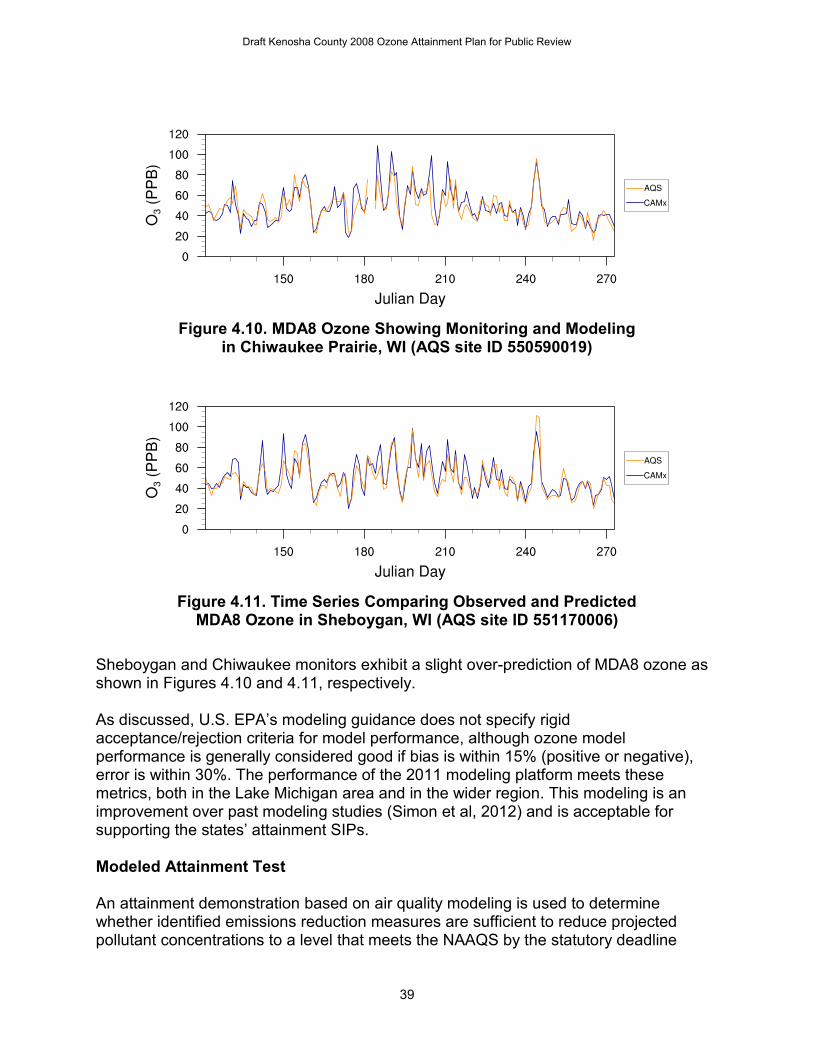
LADCO Region ...................................................................................................... 38 Figure 4.10. Time Series Comparing Observed and Predicted MDA8 Ozone in
Chiwaukee Prairie, WI ........................................................................................... 39 Figure 4.11. Time Series Comparing Observed and Predicted MDA8 Ozone in
Sheboygan, WI ..................................................................................................... 39 Figure 4.12. Coal Utilization (heat input) Projected by the ERTAC EGU
Projection Tool for Power Plants in the LADCO States that IPM Projects to be Shut Down by 2017 ....................................................................................... 42
Figure 4.13. Comparison of ERTAC and IPM 2017 NOx Emissions ........................... 43
Draft Kenosha County 2008 Ozone Attainment Plan for Public Review

iv
List of Figures (continued)
Figure 4.14. Downward Trend in U.S. Coal Net Generation Forecasts from EIA, 2008-2016 .............................................................................................. 44
Draft Kenosha County 2008 Ozone Attainment Plan for Public Review
v
List of Tables
Table 2.1. Design Values for Ozone Monitors in the Chicago and Sheboygan
Nonattainment Areas, 2010-2016 ............................................................................ 8 Table 3.1. Input Files Used by the ERTAC EGU Forecast Tool ................................. 24 Table 3.2. Evaluation of CSAPR NOx Budgets .......................................................... 27 Table 4.1. 2011 Modeling Platform Components ....................................................... 29 Table 4.2. CAMx Modeling Configuration ................................................................... 32 Table 4.3. Projected Ozone Design Values for 2017 in the Chicago and
Sheboygan Ozone Nonattainment Areas. .............................................................. 41 Table 4.4. Projected Ozone Design Values for 2017 Assuming Alternate
2011 Baseline Design Values ................................................................................ 45
Draft Kenosha County 2008 Ozone Attainment Plan for Public Review
1
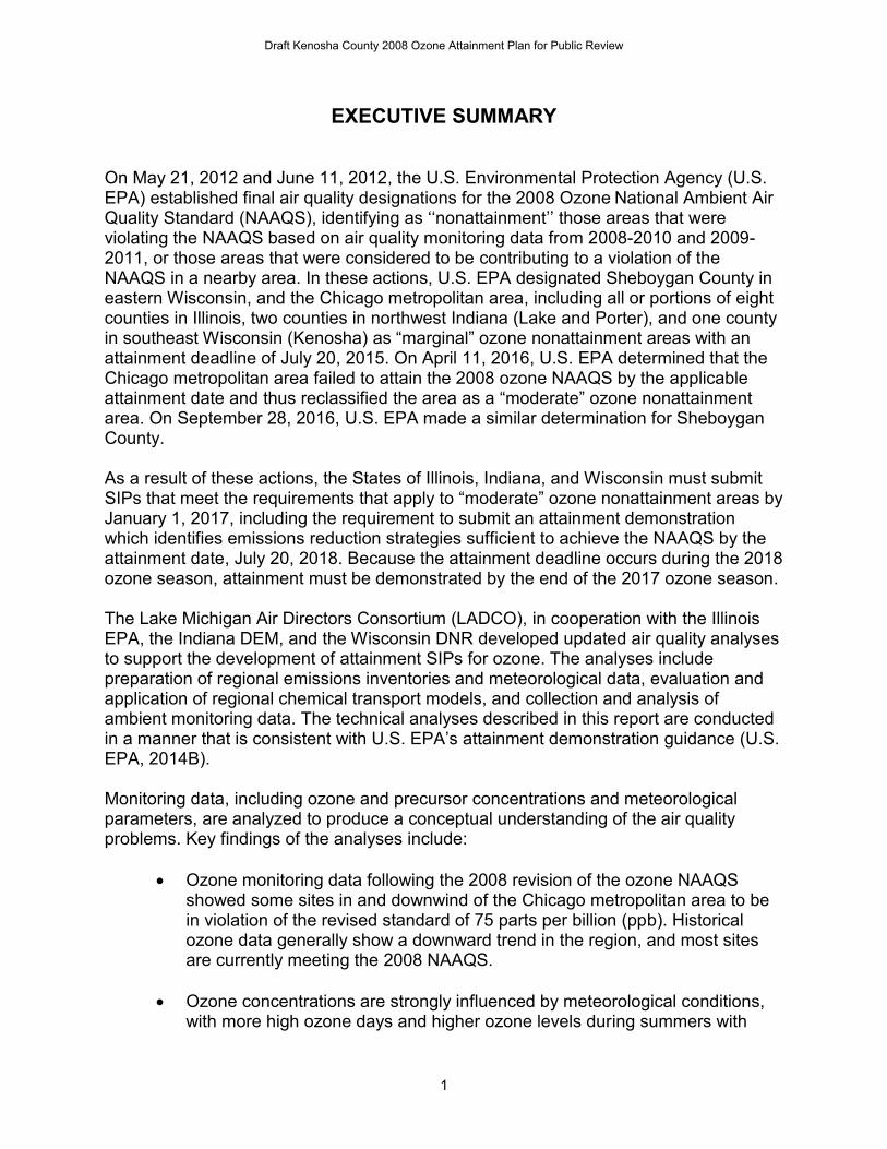
EXECUTIVE SUMMARY On May 21, 2012 and June 11, 2012, the U.S. Environmental Protection Agency (U.S. EPA) established final air quality designations for the 2008 Ozone National Ambient Air Quality Standard (NAAQS), identifying as ‘‘nonattainment’’ those areas that were violating the NAAQS based on air quality monitoring data from 2008-2010 and 2009-2011, or those areas that were considered to be contributing to a violation of the NAAQS in a nearby area. In these actions, U.S. EPA designated Sheboygan County in eastern Wisconsin, and the Chicago metropolitan area, including all or portions of eight counties in Illinois, two counties in northwest Indiana (Lake and Porter), and one county in southeast Wisconsin (Kenosha) as “marginal” ozone nonattainment areas with an attainment deadline of July 20, 2015. On April 11, 2016, U.S. EPA determined that the Chicago metropolitan area failed to attain the 2008 ozone NAAQS by the applicable attainment date and thus reclassified the area as a “moderate” ozone nonattainment area. On September 28, 2016, U.S. EPA made a similar determination for Sheboygan County. As a result of these actions, the States of Illinois, Indiana, and Wisconsin must submit SIPs that meet the requirements that apply to “moderate” ozone nonattainment areas by January 1, 2017, including the requirement to submit an attainment demonstration which identifies emissions reduction strategies sufficient to achieve the NAAQS by the attainment date, July 20, 2018. Because the attainment deadline occurs during the 2018 ozone season, attainment must be demonstrated by the end of the 2017 ozone season. The Lake Michigan Air Directors Consortium (LADCO), in cooperation with the Illinois EPA, the Indiana DEM, and the Wisconsin DNR developed updated air quality analyses to support the development of attainment SIPs for ozone. The analyses include preparation of regional emissions inventories and meteorological data, evaluation and application of regional chemical transport models, and collection and analysis of ambient monitoring data. The technical analyses described in this report are conducted in a manner that is consistent with U.S. EPA’s attainment demonstration guidance (U.S. EPA, 2014B). Monitoring data, including ozone and precursor concentrations and meteorological parameters, are analyzed to produce a conceptual understanding of the air quality problems. Key findings of the analyses include:
Ozone monitoring data following the 2008 revision of the ozone NAAQS showed some sites in and downwind of the Chicago metropolitan area to be in violation of the revised standard of 75 parts per billion (ppb). Historical ozone data generally show a downward trend in the region, and most sites are currently meeting the 2008 NAAQS.
Ozone concentrations are strongly influenced by meteorological conditions,
with more high ozone days and higher ozone levels during summers with
Draft Kenosha County 2008 Ozone Attainment Plan for Public Review
2
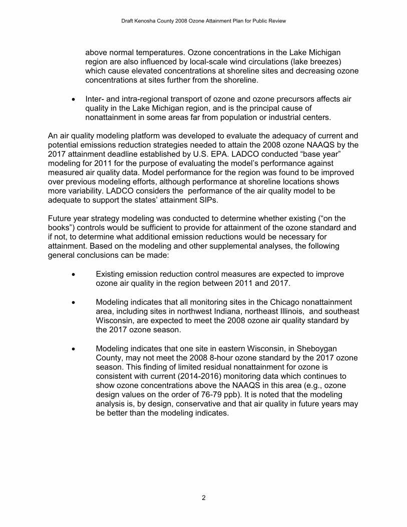
above normal temperatures. Ozone concentrations in the Lake Michigan region are also influenced by local-scale wind circulations (lake breezes) which cause elevated concentrations at shoreline sites and decreasing ozone concentrations at sites further from the shoreline.
Inter- and intra-regional transport of ozone and ozone precursors affects air
quality in the Lake Michigan region, and is the principal cause of nonattainment in some areas far from population or industrial centers.
An air quality modeling platform was developed to evaluate the adequacy of current and potential emissions reduction strategies needed to attain the 2008 ozone NAAQS by the 2017 attainment deadline established by U.S. EPA. LADCO conducted “base year” modeling for 2011 for the purpose of evaluating the model’s performance against measured air quality data. Model performance for the region was found to be improved over previous modeling efforts, although performance at shoreline locations shows more variability. LADCO considers the performance of the air quality model to be adequate to support the states’ attainment SIPs. Future year strategy modeling was conducted to determine whether existing (“on the books”) controls would be sufficient to provide for attainment of the ozone standard and if not, to determine what additional emission reductions would be necessary for attainment. Based on the modeling and other supplemental analyses, the following general conclusions can be made:
Existing emission reduction control measures are expected to improve ozone air quality in the region between 2011 and 2017.
Modeling indicates that all monitoring sites in the Chicago nonattainment
area, including sites in northwest Indiana, northeast Illinois, and southeast Wisconsin, are expected to meet the 2008 ozone air quality standard by the 2017 ozone season.
Modeling indicates that one site in eastern Wisconsin, in Sheboygan County, may not meet the 2008 8-hour ozone standard by the 2017 ozone season. This finding of limited residual nonattainment for ozone is consistent with current (2014-2016) monitoring data which continues to show ozone concentrations above the NAAQS in this area (e.g., ozone design values on the order of 76-79 ppb). It is noted that the modeling analysis is, by design, conservative and that air quality in future years may be better than the modeling indicates.
Draft Kenosha County 2008 Ozone Attainment Plan for Public Review
3
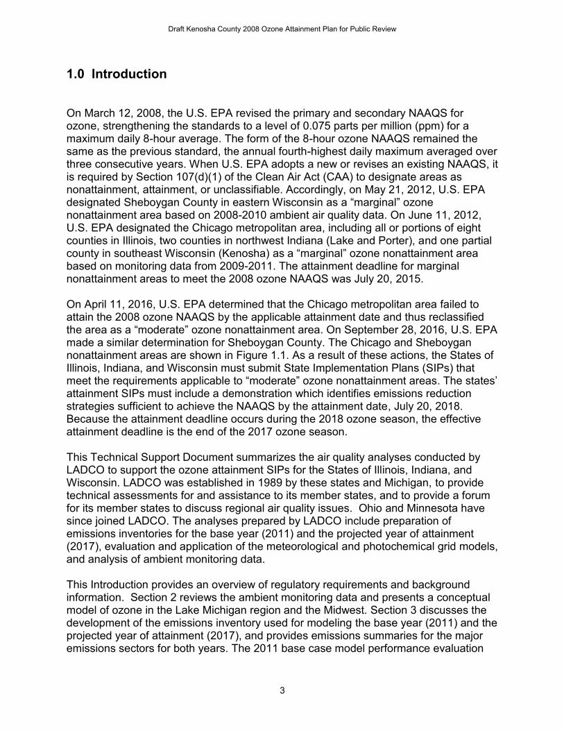
1.0 Introduction On March 12, 2008, the U.S. EPA revised the primary and secondary NAAQS for ozone, strengthening the standards to a level of 0.075 parts per million (ppm) for a maximum daily 8-hour average. The form of the 8-hour ozone NAAQS remained the same as the previous standard, the annual fourth-highest daily maximum averaged over three consecutive years. When U.S. EPA adopts a new or revises an existing NAAQS, it is required by Section 107(d)(1) of the Clean Air Act (CAA) to designate areas as nonattainment, attainment, or unclassifiable. Accordingly, on May 21, 2012, U.S. EPA designated Sheboygan County in eastern Wisconsin as a “marginal” ozone nonattainment area based on 2008-2010 ambient air quality data. On June 11, 2012, U.S. EPA designated the Chicago metropolitan area, including all or portions of eight counties in Illinois, two counties in northwest Indiana (Lake and Porter), and one partial county in southeast Wisconsin (Kenosha) as a “marginal” ozone nonattainment area based on monitoring data from 2009-2011. The attainment deadline for marginal nonattainment areas to meet the 2008 ozone NAAQS was July 20, 2015. On April 11, 2016, U.S. EPA determined that the Chicago metropolitan area failed to attain the 2008 ozone NAAQS by the applicable attainment date and thus reclassified the area as a “moderate” ozone nonattainment area. On September 28, 2016, U.S. EPA made a similar determination for Sheboygan County. The Chicago and Sheboygan nonattainment areas are shown in Figure 1.1. As a result of these actions, the States of Illinois, Indiana, and Wisconsin must submit State Implementation Plans (SIPs) that meet the requirements applicable to “moderate” ozone nonattainment areas. The states’ attainment SIPs must include a demonstration which identifies emissions reduction strategies sufficient to achieve the NAAQS by the attainment date, July 20, 2018. Because the attainment deadline occurs during the 2018 ozone season, the effective attainment deadline is the end of the 2017 ozone season. This Technical Support Document summarizes the air quality analyses conducted by LADCO to support the ozone attainment SIPs for the States of Illinois, Indiana, and Wisconsin. LADCO was established in 1989 by these states and Michigan, to provide technical assessments for and assistance to its member states, and to provide a forum for its member states to discuss regional air quality issues. Ohio and Minnesota have since joined LADCO. The analyses prepared by LADCO include preparation of emissions inventories for the base year (2011) and the projected year of attainment (2017), evaluation and application of the meteorological and photochemical grid models, and analysis of ambient monitoring data. This Introduction provides an overview of regulatory requirements and background information. Section 2 reviews the ambient monitoring data and presents a conceptual model of ozone in the Lake Michigan region and the Midwest. Section 3 discusses the development of the emissions inventory used for modeling the base year (2011) and the projected year of attainment (2017), and provides emissions summaries for the major emissions sectors for both years. The 2011 base case model performance evaluation
Draft Kenosha County 2008 Ozone Attainment Plan for Public Review
4
Figure 1.1. Nonattainment Areas in the Lake Michigan Region for the 2008 Ozone National Ambient Air Quality Standard
and the modeling assessment for 2017 are presented in Section 4, along with relevant analyses considered as part of the weight-of-evidence determination. Finally, key study findings are reviewed and summarized in Section 5. SIP Requirements As mentioned previously, U.S. EPA designated Sheboygan County in eastern Wisconsin, and the Chicago metropolitan area, including portions of northeast Illinois,
Draft Kenosha County 2008 Ozone Attainment Plan for Public Review
5
northwest Indiana, and southeast Wisconsin, as “marginal” ozone nonattainment areas for the 2008 8-hour ozone NAAQS. Based on a finding of failure to attain by the applicable attainment date, U.S. EPA subsequently reclassified the Chicago and Sheboygan nonattainment areas as “moderate” ozone nonattainment areas. The states must therefore meet the requirements that apply to “moderate” ozone nonattainment areas, including the following:
Nonattainment New Source Review, with emissions offsets for new or modified sources at a ratio of 1.15 to 1 tons of emissions;
Reasonably Available Control Technology (RACT) for existing VOC and NOx emissions sources in the nonattainment areas;
Additional reductions of VOCs or NOx necessary for the state to demonstrate 15% reduction from baseline emissions within six years;
Emission reduction measures needed to attain, as demonstrated by a formal modeled attainment demonstration.
This Technical Support Document identifies emissions reduction strategies and includes a modeling assessment of the effectiveness of the strategies in achieving the NAAQS. The states must submit attainment SIPs to U.S. EPA by January 1, 2017. The deadline for meeting the 8-hour ozone NAAQS is July 20, 2018. Because the attainment deadline occurs during the 2018 ozone season, the effective attainment deadline is the end of the 2017 ozone season. Technical Work: Overview LADCO worked closely with the States of Illinois, Indiana, and Wisconsin and U.S. EPA Region 5 to develop the technical analyses described in this report. A “conceptual model” is presented which provides a qualitative description of the region’s ozone air quality, based on an analysis of ambient air quality data. These analyses also provide information for evaluating the performance of the air quality model. The data analyses are an integral part of the overall technical support given uncertainties in emissions inventories and modeling. Base year (2011) and future year (2017) emissions inventories are based on U.S. EPA’s modeling platforms, as described in U.S. EPA’s “Notice of Availability of the Environmental Protection Agency’s Updated Ozone Transport Modeling Data for the 2008 Ozone National Ambient Air Quality Standard (NAAQS)” (U.S. EPA, 2015A). States provided point source and area source emissions data, and MOVES input files and mobile source activity data to U.S. EPA’s 2011 National Emissions Inventory (NEI) database. U.S. EPA prepared emissions data for other categories not provided by the states, including nonroad sources, ammonia, fires, and biogenics. LADCO and its contractors developed improved emissions data for its member states for on-road sources and electrical generating units. The air quality modeling described here can act as the core of states’ attainment demonstrations. The modeling methodology described in this Technical Support
Draft Kenosha County 2008 Ozone Attainment Plan for Public Review
6
Document adheres to U.S. EPA’s guidance document: “Draft Modeling Guidance for Demonstrating Attainment of Air Quality Goals for Ozone, PM2.5, and Regional Haze” (U.S. EPA, 2014B). LADCO used a combination of models and specified methods to model air quality for an attainment assessment. These included the Weather Research and Forecasting (WRF) model, the Sparse Matrix Operator Kernel Emissions (SMOKE) modeling system, the Eastern Regional Technical Advisory Committee (ERTAC) EGU Forecast Tool, and the Comprehensive Air quality Model with extensions (CAMx). These models and tools are described in greater detail in Sections 3 and 4.
The models used in this technical analysis meet all of the prerequisites stated in U.S. EPA’s draft modeling guidance.
Draft Kenosha County 2008 Ozone Attainment Plan for Public Review
7
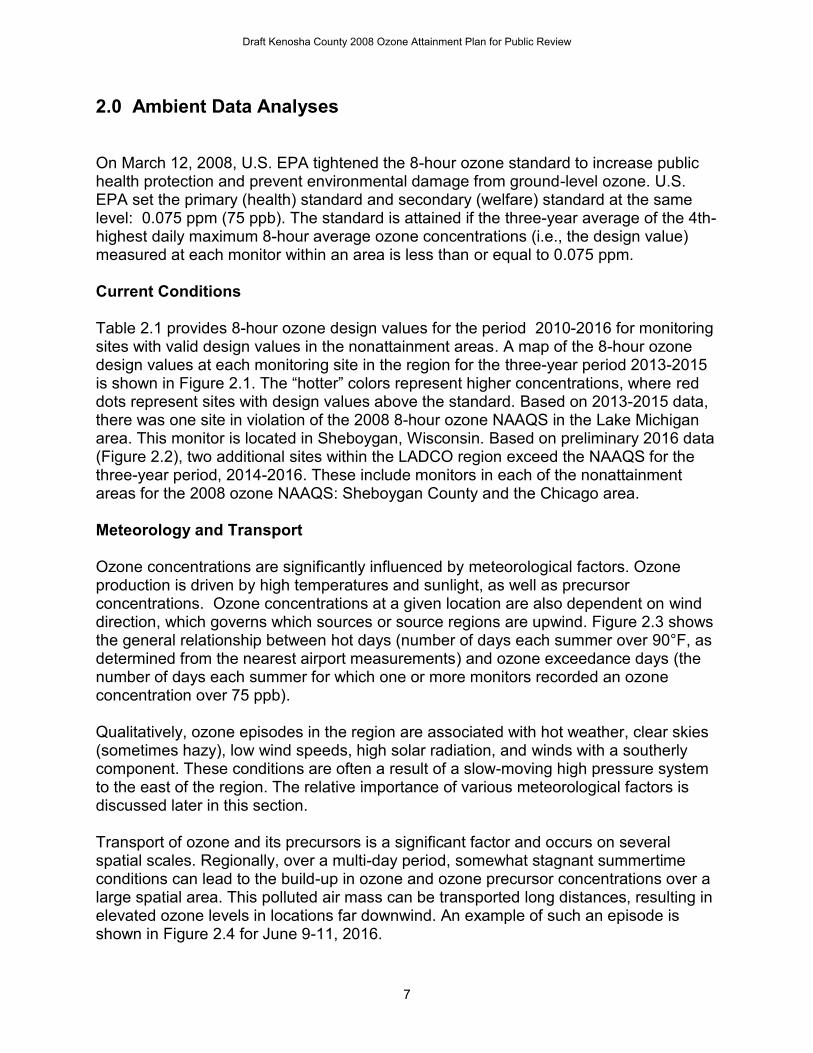
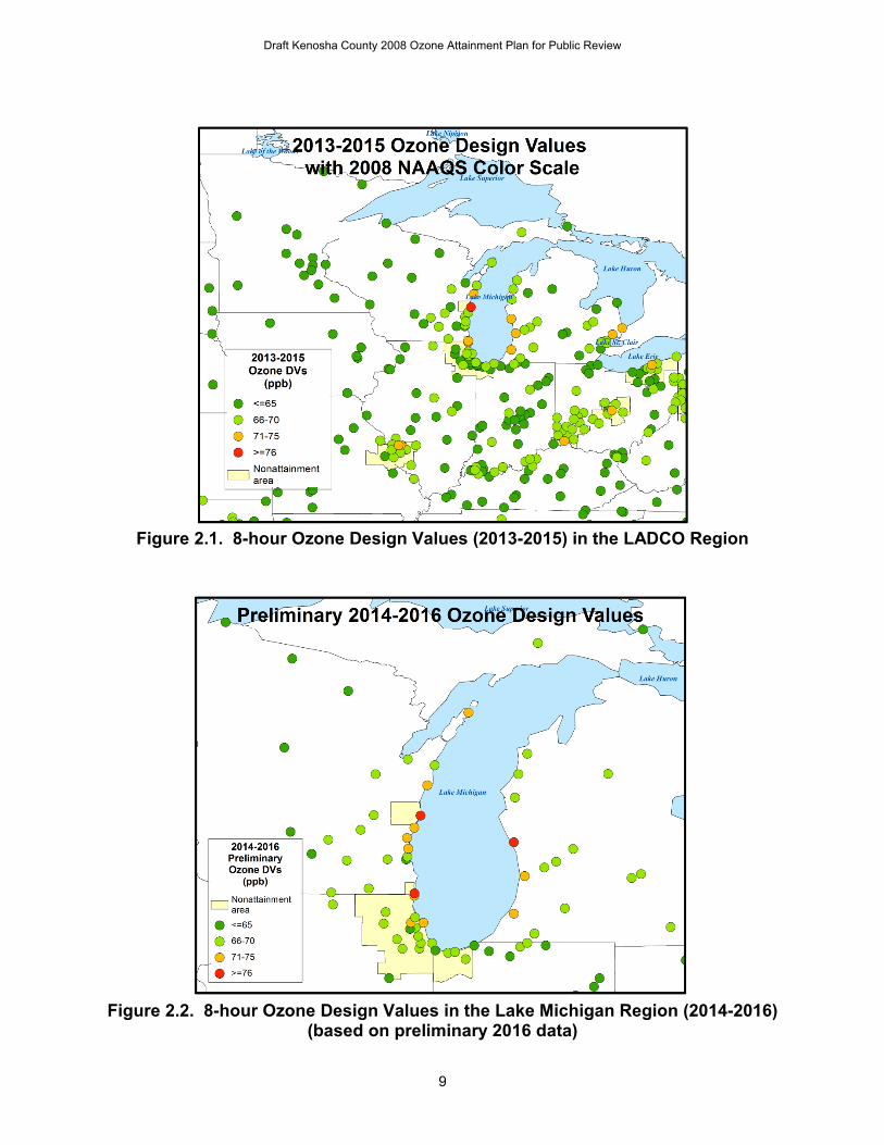
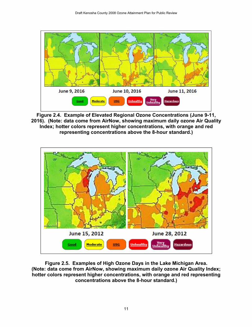
2.0 Ambient Data Analyses On March 12, 2008, U.S. EPA tightened the 8-hour ozone standard to increase public health protection and prevent environmental damage from ground-level ozone. U.S. EPA set the primary (health) standard and secondary (welfare) standard at the same level: 0.075 ppm (75 ppb). The standard is attained if the three-year average of the 4th-highest daily maximum 8-hour average ozone concentrations (i.e., the design value) measured at each monitor within an area is less than or equal to 0.075 ppm. Current Conditions Table 2.1 provides 8-hour ozone design values for the period 2010-2016 for monitoring sites with valid design values in the nonattainment areas. A map of the 8-hour ozone design values at each monitoring site in the region for the three-year period 2013-2015 is shown in Figure 2.1. The “hotter” colors represent higher concentrations, where red dots represent sites with design values above the standard. Based on 2013-2015 data, there was one site in violation of the 2008 8-hour ozone NAAQS in the Lake Michigan area. This monitor is located in Sheboygan, Wisconsin. Based on preliminary 2016 data (Figure 2.2), two additional sites within the LADCO region exceed the NAAQS for the three-year period, 2014-2016. These include monitors in each of the nonattainment areas for the 2008 ozone NAAQS: Sheboygan County and the Chicago area. Meteorology and Transport Ozone concentrations are significantly influenced by meteorological factors. Ozone production is driven by high temperatures and sunlight, as well as precursor concentrations. Ozone concentrations at a given location are also dependent on wind direction, which governs which sources or source regions are upwind. Figure 2.3 shows the general relationship between hot days (number of days each summer over 90°F, as determined from the nearest airport measurements) and ozone exceedance days (the number of days each summer for which one or more monitors recorded an ozone concentration over 75 ppb). Qualitatively, ozone episodes in the region are associated with hot weather, clear skies (sometimes hazy), low wind speeds, high solar radiation, and winds with a southerly component. These conditions are often a result of a slow-moving high pressure system to the east of the region. The relative importance of various meteorological factors is discussed later in this section. Transport of ozone and its precursors is a significant factor and occurs on several spatial scales. Regionally, over a multi-day period, somewhat stagnant summertime conditions can lead to the build-up in ozone and ozone precursor concentrations over a large spatial area. This polluted air mass can be transported long distances, resulting in elevated ozone levels in locations far downwind. An example of such an episode is shown in Figure 2.4 for June 9-11, 2016.
Draft Kenosha County 2008 Ozone Attainment Plan for Public Review
8
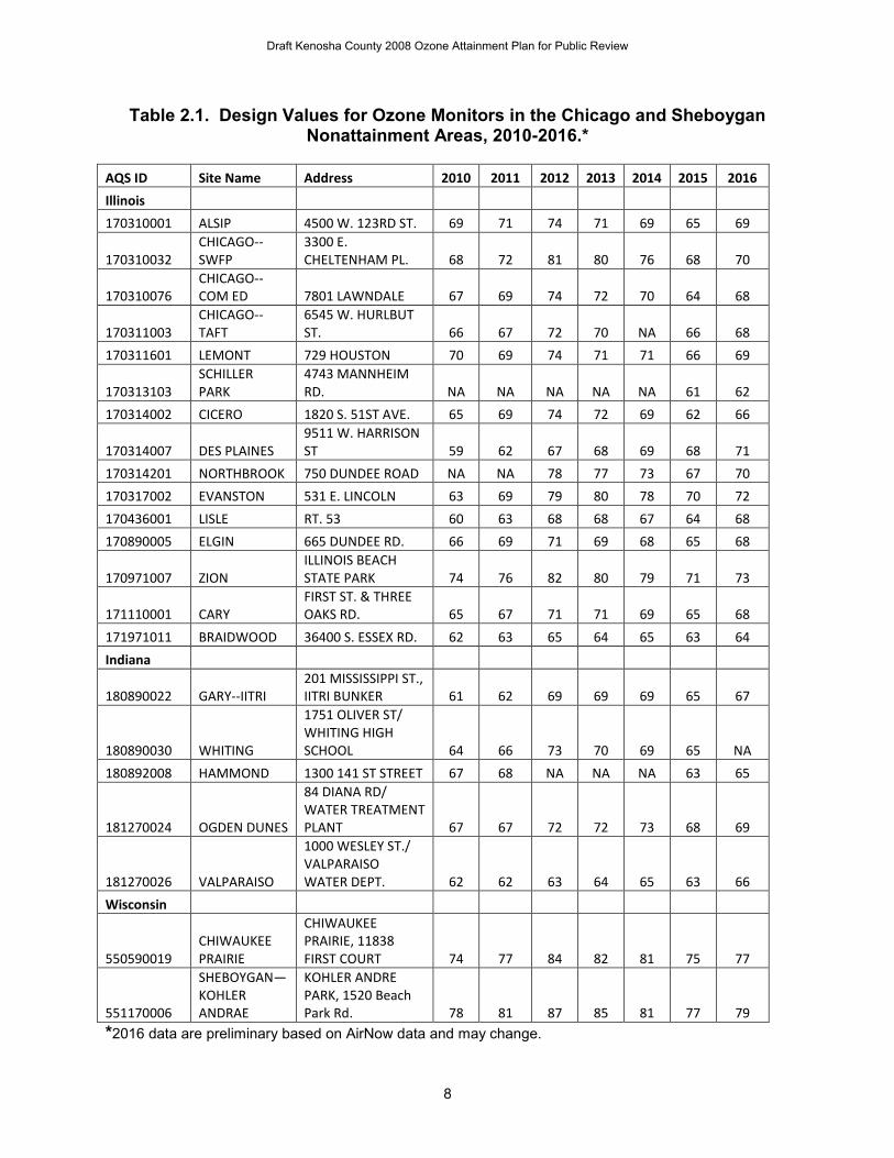
Table 2.1. Design Values for Ozone Monitors in the Chicago and Sheboygan Nonattainment Areas, 2010-2016.*
AQS ID Site Name Address 2010 2011 2012 2013 2014 2015 2016
Illinois
170310001 ALSIP 4500 W. 123RD ST. 69 71 74 71 69 65 69
170310032 CHICAGO--SWFP
3300 E. CHELTENHAM PL. 68 72 81 80 76 68 70
170310076 CHICAGO--COM ED 7801 LAWNDALE 67 69 74 72 70 64 68
170311003 CHICAGO--TAFT
6545 W. HURLBUT ST. 66 67 72 70 NA 66 68
170311601 LEMONT 729 HOUSTON 70 69 74 71 71 66 69
170313103 SCHILLER PARK
4743 MANNHEIM RD. NA NA NA NA NA 61 62
170314002 CICERO 1820 S. 51ST AVE. 65 69 74 72 69 62 66
170314007 DES PLAINES 9511 W. HARRISON ST 59 62 67 68 69 68 71
170314201 NORTHBROOK 750 DUNDEE ROAD NA NA 78 77 73 67 70
170317002 EVANSTON 531 E. LINCOLN 63 69 79 80 78 70 72
170436001 LISLE RT. 53 60 63 68 68 67 64 68
170890005 ELGIN 665 DUNDEE RD. 66 69 71 69 68 65 68
170971007 ZION ILLINOIS BEACH STATE PARK 74 76 82 80 79 71 73
171110001 CARY FIRST ST. & THREE OAKS RD. 65 67 71 71 69 65 68
171971011 BRAIDWOOD 36400 S. ESSEX RD. 62 63 65 64 65 63 64
Indiana
180890022 GARY--IITRI 201 MISSISSIPPI ST., IITRI BUNKER 61 62 69 69 69 65 67
180890030 WHITING
1751 OLIVER ST/ WHITING HIGH SCHOOL 64 66 73 70 69 65 NA
180892008 HAMMOND 1300 141 ST STREET 67 68 NA NA NA 63 65
181270024 OGDEN DUNES
84 DIANA RD/ WATER TREATMENT PLANT 67 67 72 72 73 68 69
181270026 VALPARAISO
1000 WESLEY ST./ VALPARAISO WATER DEPT. 62 62 63 64 65 63 66
Wisconsin
550590019 CHIWAUKEE PRAIRIE
CHIWAUKEE PRAIRIE, 11838 FIRST COURT 74 77 84 82 81 75 77
551170006
SHEBOYGAN—KOHLER ANDRAE
KOHLER ANDRE PARK, 1520 Beach Park Rd. 78 81 87 85 81 77 79
*2016 data are preliminary based on AirNow data and may change.
Draft Kenosha County 2008 Ozone Attainment Plan for Public Review
9
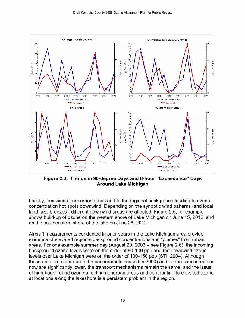
Figure 2.1. 8-hour Ozone Design Values (2013-2015) in the LADCO Region
Figure 2.2. 8-hour Ozone Design Values in the Lake Michigan Region (2014-2016)
(based on preliminary 2016 data)
Draft Kenosha County 2008 Ozone Attainment Plan for Public Review
10
Figure 2.3. Trends in 90-degree Days and 8-hour “Exceedance” Days
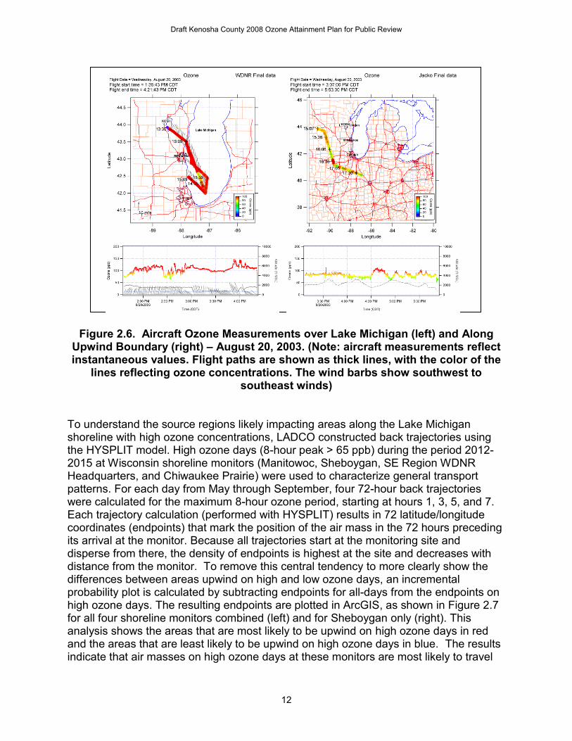
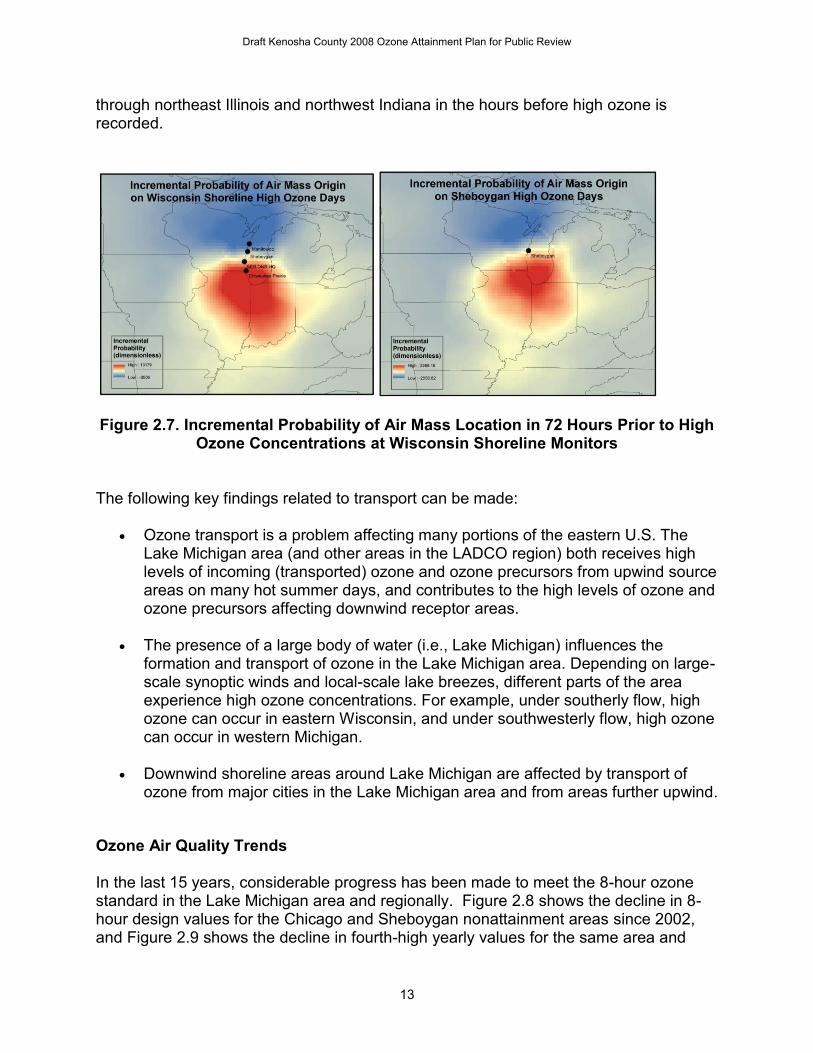
Around Lake Michigan Locally, emissions from urban areas add to the regional background leading to ozone concentration hot spots downwind. Depending on the synoptic wind patterns (and local land-lake breezes), different downwind areas are affected. Figure 2.5, for example, shows build-up of ozone on the western shore of Lake Michigan on June 15, 2012, and on the southeastern shore of the lake on June 28, 2012. Aircraft measurements conducted in prior years in the Lake Michigan area provide evidence of elevated regional background concentrations and “plumes” from urban areas. For one example summer day (August 20, 2003 – see Figure 2.6), the incoming background ozone levels were on the order of 80-100 ppb and the downwind ozone levels over Lake Michigan were on the order of 100-150 ppb (STI, 2004). Although these data are older (aircraft measurements ceased in 2003) and ozone concentrations now are significantly lower, the transport mechanisms remain the same, and the issue of high background ozone affecting nonurban areas and contributing to elevated ozone at locations along the lakeshore is a persistent problem in the region.
Draft Kenosha County 2008 Ozone Attainment Plan for Public Review
11
Figure 2.4. Example of Elevated Regional Ozone Concentrations (June 9-11,
2016). (Note: data come from AirNow, showing maximum daily ozone Air Quality Index; hotter colors represent higher concentrations, with orange and red
representing concentrations above the 8-hour standard.)
Figure 2.5. Examples of High Ozone Days in the Lake Michigan Area. (Note: data come from AirNow, showing maximum daily ozone Air Quality Index; hotter colors represent higher concentrations, with orange and red representing
concentrations above the 8-hour standard.)
Draft Kenosha County 2008 Ozone Attainment Plan for Public Review
12
Figure 2.6. Aircraft Ozone Measurements over Lake Michigan (left) and Along Upwind Boundary (right) – August 20, 2003. (Note: aircraft measurements reflect instantaneous values. Flight paths are shown as thick lines, with the color of the
lines reflecting ozone concentrations. The wind barbs show southwest to southeast winds)
To understand the source regions likely impacting areas along the Lake Michigan shoreline with high ozone concentrations, LADCO constructed back trajectories using the HYSPLIT model. High ozone days (8-hour peak > 65 ppb) during the period 2012-2015 at Wisconsin shoreline monitors (Manitowoc, Sheboygan, SE Region WDNR Headquarters, and Chiwaukee Prairie) were used to characterize general transport patterns. For each day from May through September, four 72-hour back trajectories were calculated for the maximum 8-hour ozone period, starting at hours 1, 3, 5, and 7. Each trajectory calculation (performed with HYSPLIT) results in 72 latitude/longitude coordinates (endpoints) that mark the position of the air mass in the 72 hours preceding its arrival at the monitor. Because all trajectories start at the monitoring site and disperse from there, the density of endpoints is highest at the site and decreases with distance from the monitor. To remove this central tendency to more clearly show the differences between areas upwind on high and low ozone days, an incremental probability plot is calculated by subtracting endpoints for all-days from the endpoints on high ozone days. The resulting endpoints are plotted in ArcGIS, as shown in Figure 2.7 for all four shoreline monitors combined (left) and for Sheboygan only (right). This analysis shows the areas that are most likely to be upwind on high ozone days in red and the areas that are least likely to be upwind on high ozone days in blue. The results indicate that air masses on high ozone days at these monitors are most likely to travel
Draft Kenosha County 2008 Ozone Attainment Plan for Public Review
13
through northeast Illinois and northwest Indiana in the hours before high ozone is recorded.
Figure 2.7. Incremental Probability of Air Mass Location in 72 Hours Prior to High Ozone Concentrations at Wisconsin Shoreline Monitors
The following key findings related to transport can be made:
Ozone transport is a problem affecting many portions of the eastern U.S. The Lake Michigan area (and other areas in the LADCO region) both receives high levels of incoming (transported) ozone and ozone precursors from upwind source areas on many hot summer days, and contributes to the high levels of ozone and ozone precursors affecting downwind receptor areas.
The presence of a large body of water (i.e., Lake Michigan) influences the
formation and transport of ozone in the Lake Michigan area. Depending on large-scale synoptic winds and local-scale lake breezes, different parts of the area experience high ozone concentrations. For example, under southerly flow, high ozone can occur in eastern Wisconsin, and under southwesterly flow, high ozone can occur in western Michigan.
Downwind shoreline areas around Lake Michigan are affected by transport of
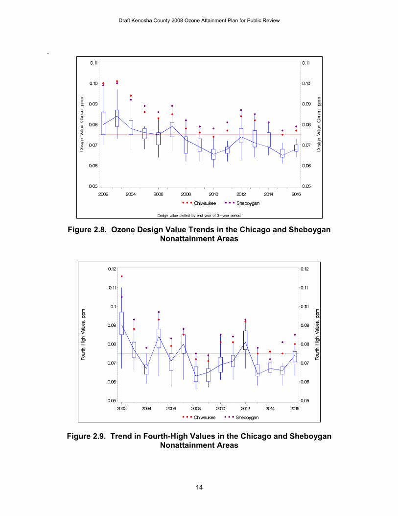
ozone from major cities in the Lake Michigan area and from areas further upwind. Ozone Air Quality Trends In the last 15 years, considerable progress has been made to meet the 8-hour ozone standard in the Lake Michigan area and regionally. Figure 2.8 shows the decline in 8-hour design values for the Chicago and Sheboygan nonattainment areas since 2002, and Figure 2.9 shows the decline in fourth-high yearly values for the same area and
Draft Kenosha County 2008 Ozone Attainment Plan for Public Review
14
.
Figure 2.8. Ozone Design Value Trends in the Chicago and Sheboygan
Nonattainment Areas
Figure 2.9. Trend in Fourth-High Values in the Chicago and Sheboygan Nonattainment Areas
Draft Kenosha County 2008 Ozone Attainment Plan for Public Review
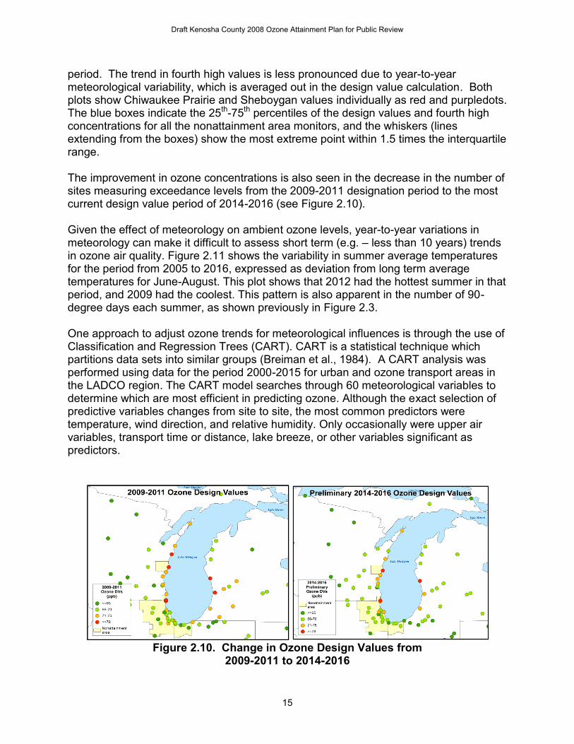
15
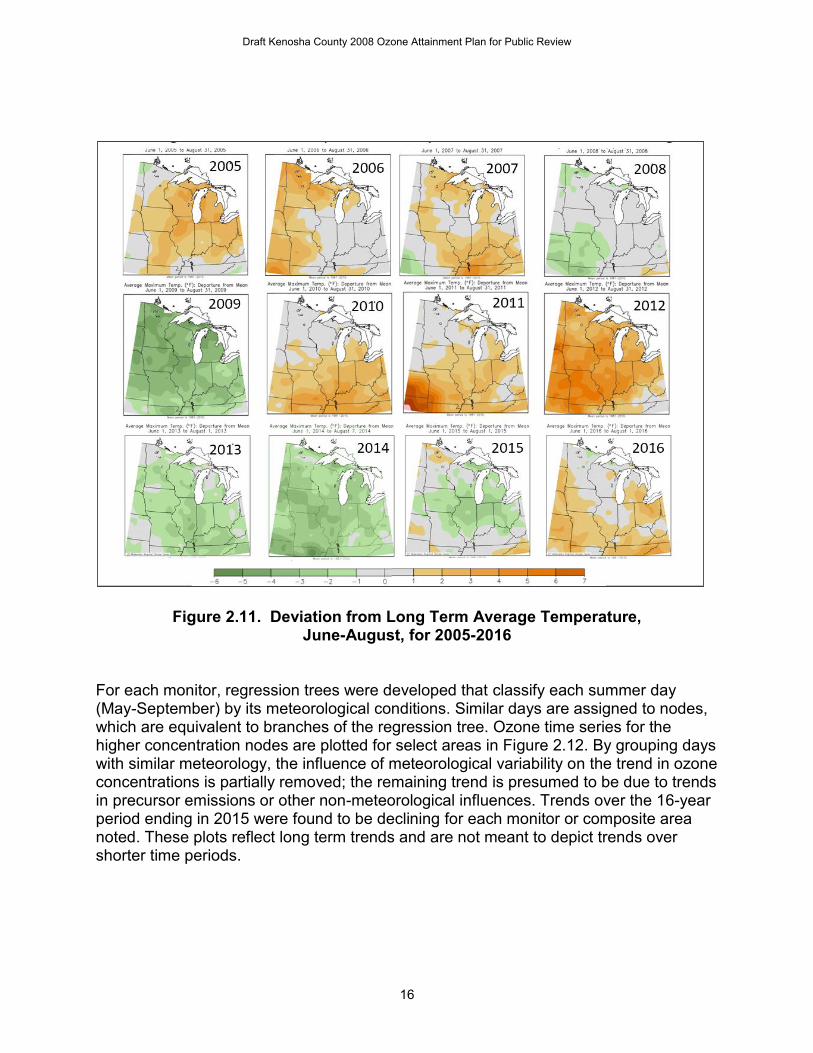
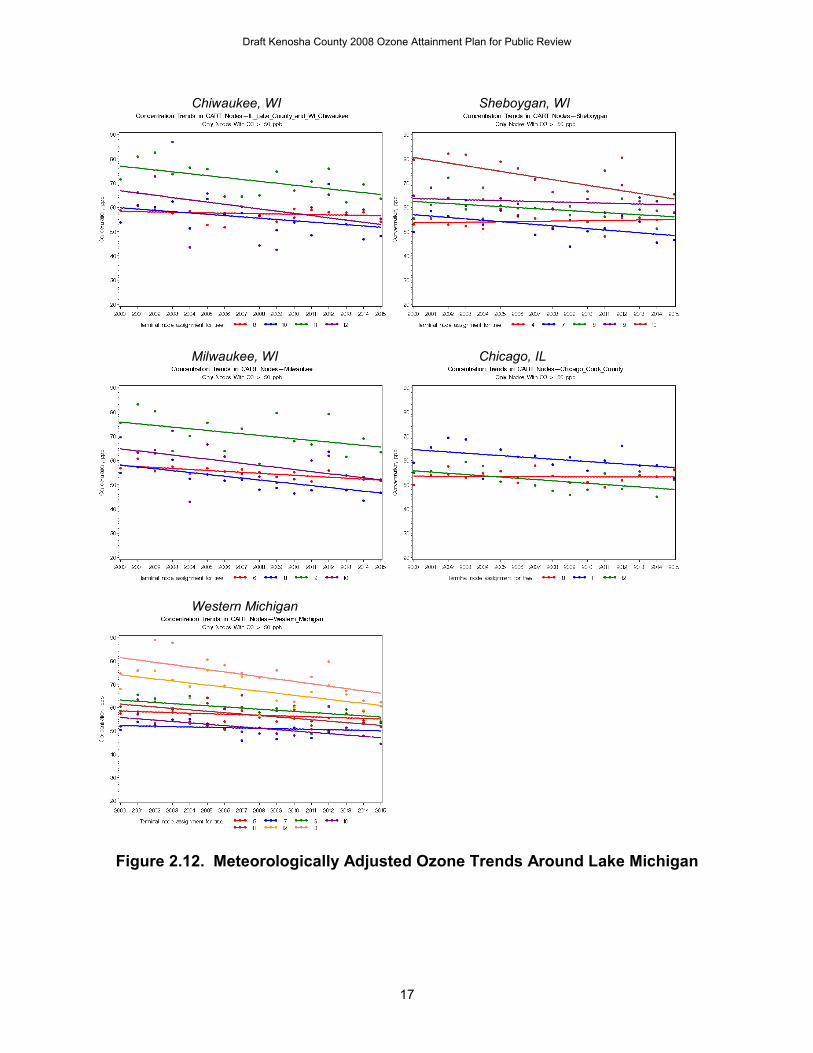
period. The trend in fourth high values is less pronounced due to year-to-year meteorological variability, which is averaged out in the design value calculation. Both plots show Chiwaukee Prairie and Sheboygan values individually as red and purpledots. The blue boxes indicate the 25th-75th percentiles of the design values and fourth high concentrations for all the nonattainment area monitors, and the whiskers (lines extending from the boxes) show the most extreme point within 1.5 times the interquartile range. The improvement in ozone concentrations is also seen in the decrease in the number of sites measuring exceedance levels from the 2009-2011 designation period to the most current design value period of 2014-2016 (see Figure 2.10). Given the effect of meteorology on ambient ozone levels, year-to-year variations in meteorology can make it difficult to assess short term (e.g. – less than 10 years) trends in ozone air quality. Figure 2.11 shows the variability in summer average temperatures for the period from 2005 to 2016, expressed as deviation from long term average temperatures for June-August. This plot shows that 2012 had the hottest summer in that period, and 2009 had the coolest. This pattern is also apparent in the number of 90-degree days each summer, as shown previously in Figure 2.3. One approach to adjust ozone trends for meteorological influences is through the use of Classification and Regression Trees (CART). CART is a statistical technique which partitions data sets into similar groups (Breiman et al., 1984). A CART analysis was performed using data for the period 2000-2015 for urban and ozone transport areas in the LADCO region. The CART model searches through 60 meteorological variables to determine which are most efficient in predicting ozone. Although the exact selection of predictive variables changes from site to site, the most common predictors were temperature, wind direction, and relative humidity. Only occasionally were upper air variables, transport time or distance, lake breeze, or other variables significant as predictors.
Figure 2.10. Change in Ozone Design Values from
2009-2011 to 2014-2016
Draft Kenosha County 2008 Ozone Attainment Plan for Public Review
16
Figure 2.11. Deviation from Long Term Average Temperature, June-August, for 2005-2016
For each monitor, regression trees were developed that classify each summer day (May-September) by its meteorological conditions. Similar days are assigned to nodes, which are equivalent to branches of the regression tree. Ozone time series for the higher concentration nodes are plotted for select areas in Figure 2.12. By grouping days with similar meteorology, the influence of meteorological variability on the trend in ozone concentrations is partially removed; the remaining trend is presumed to be due to trends in precursor emissions or other non-meteorological influences. Trends over the 16-year period ending in 2015 were found to be declining for each monitor or composite area noted. These plots reflect long term trends and are not meant to depict trends over shorter time periods.
Draft Kenosha County 2008 Ozone Attainment Plan for Public Review
17
Chiwaukee, WI Sheboygan, WI
Milwaukee, WI Chicago, IL
Western Michigan
Figure 2.12. Meteorologically Adjusted Ozone Trends Around Lake Michigan
Draft Kenosha County 2008 Ozone Attainment Plan for Public Review

18
Conceptual Model for Ozone in the Lake Michigan Region A conceptual model is a qualitative summary of the physical, chemical, and meteorological processes that control the formation and distribution of pollutants in a given region. Based on the data and analyses presented above, and of previous conceptual models and technical support documents developed for the Lake Michigan region, a conceptual model of the behavior, meteorological influences, and causes of high ozone in the Chicago and Sheboygan nonattainment areas is summarized below:
Current monitoring data show that most sites in the Lake Michigan region are meeting the 2008 8-hour ozone NAAQS. However, three sites in the region exceeded the 8-hour ozone standard of 75 ppb in 2014-16: Chiwaukee Prairie, WI, Sheboygan, WI, and Muskegon, MI. Historical ozone data show a downward trend over the past 15 years, due likely to federal and state emission control programs. Concentrations declined sharply from 2002 through 2010. The rate of decrease appears to have tapered in recent years, although the high year-to-year variability of ozone makes it imprudent to make assumptions about short-term trends.
Ozone concentrations are strongly influenced by meteorological conditions,
with more high ozone days and higher ozone levels during summers with above normal temperatures. Nevertheless, meteorologically adjusted trends show that concentrations have declined even on hot days, providing strong evidence that emission reductions of ozone precursors have been effective.
Inter- and intra-regional transport of ozone and ozone precursors affects
many portions of the LADCO states, and is the principal cause of nonattainment in some areas far from population or industrial centers.
The presence of Lake Michigan influences the formation, transport, and
duration of elevated ozone concentrations along its shoreline. Depending on large-scale synoptic winds and local-scale lake breezes, different parts of the area experience high ozone concentrations. For example, under southerly flow, high ozone can occur in eastern Wisconsin, and under southwesterly flow, high ozone can occur in western Michigan.
Areas in closer proximity to the Lake shoreline display the most frequent and
most elevated ozone concentrations.
Ozone concentrations have declined since 2000-2002 both inland and along the Lake Michigan shoreline.
Draft Kenosha County 2008 Ozone Attainment Plan for Public Review
19
3.0 Emissions Inventory Development This technical analysis relies heavily on emissions and other model inputs prepared by U.S. EPA. U.S. EPA and LADCO rigorously quality assure their emission inventories (U.S. EPA, 2015A). LADCO’s emissions modeling quality assurance procedures include reviewing emissions model output files for errors and warnings, comparing emissions between processing steps, checking that speciation, temporal, and spatial allocation factors are applied correctly, and reviewing the air quality model emissions inputs and stack parameters. U.S. EPA’s Modeling Platform LADCO utilized emissions inventories compiled by U.S. EPA for the years 2011 and 2017 as the starting point for the modeling inventories used in this analysis. U.S. EPA’s 2011 emission inventory (Version 2011EH) is based on the 2011 National Emissions Inventory, version 2 (2011NEIv2), which was speciated, temporalized and gridded to provide hourly emissions inputs to support photochemical modeling. The major sectors of the anthropogenic emissions inventory are:
Electric generating units (EGUs) include fossil fuel electricity generation. Coal-fired utilities dominate this sector. These sources are defined by discrete stack locations.
Point sources (point non-EGU) include other industrial sources that do not generate power. This category includes refineries, steel mills, foundries, cement plants and other large industrial facilities.
Onroad mobile sources (Onroad) includes all onroad transportation related vehicles. Passenger automobiles and medium and heavy freight trucks are the primary vehicles included in this category.
Nonroad mobile sources (Nonroad) include small and medium engines that are not used on roadways. Examples include lawn and garden equipment, recreational marine, ATVs, and construction equipment. It also includes industrial freight handling equipment such as forklifts and cranes.
Area sources (Area) are those sources that do not fit into other groups and are spatially diverse in nature. Examples include small industrial activities, consumer solvents, home heating, and commercial and institutional fuel use.
Marine, aircraft and rail (MAR) includes commercial marine vessels, commercial and private aircraft, and railroad locomotives including those operated at switching yards.
Non-anthropogenic sources such as biogenic emissions and wildfires are also represented in the emissions inventory. For the biggest inventory sectors, the Version 2011 EH inventory relies on hourly 2011 continuous emissions monitoring system (CEMS) data for EGU emissions, hourly on-road mobile emissions, and 2011 day-
Draft Kenosha County 2008 Ozone Attainment Plan for Public Review
20
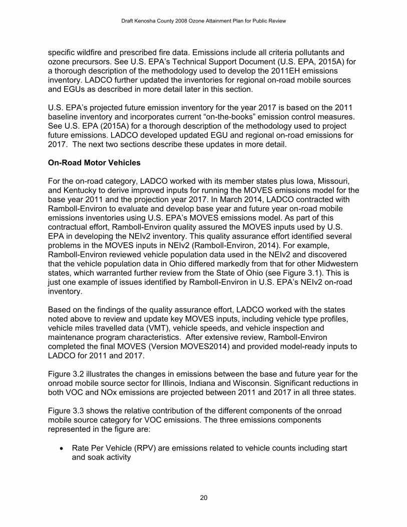
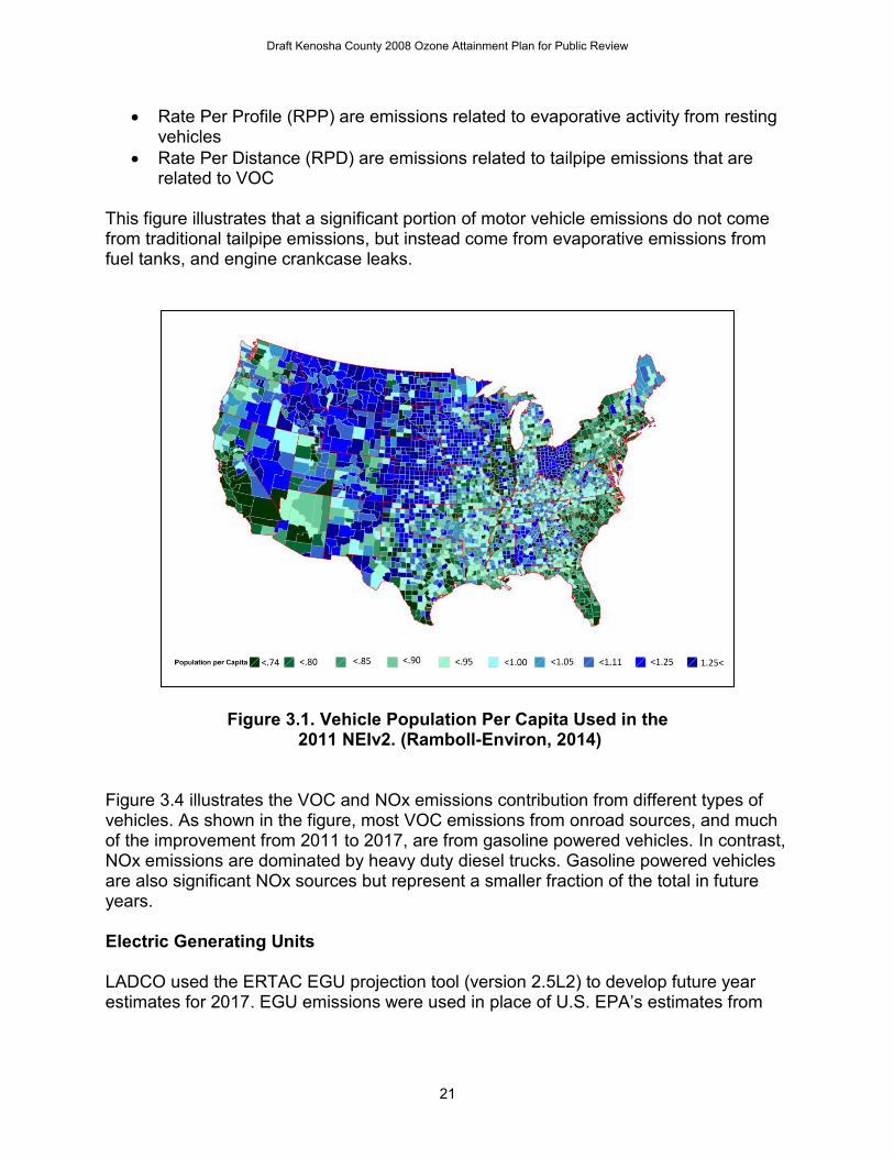
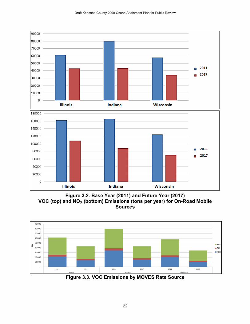
specific wildfire and prescribed fire data. Emissions include all criteria pollutants and ozone precursors. See U.S. EPA’s Technical Support Document (U.S. EPA, 2015A) for a thorough description of the methodology used to develop the 2011EH emissions inventory. LADCO further updated the inventories for regional on-road mobile sources and EGUs as described in more detail later in this section. U.S. EPA’s projected future emission inventory for the year 2017 is based on the 2011 baseline inventory and incorporates current “on-the-books” emission control measures. See U.S. EPA (2015A) for a thorough description of the methodology used to project future emissions. LADCO developed updated EGU and regional on-road emissions for 2017. The next two sections describe these updates in more detail. On-Road Motor Vehicles For the on-road category, LADCO worked with its member states plus Iowa, Missouri, and Kentucky to derive improved inputs for running the MOVES emissions model for the base year 2011 and the projection year 2017. In March 2014, LADCO contracted with Ramboll-Environ to evaluate and develop base year and future year on-road mobile emissions inventories using U.S. EPA’s MOVES emissions model. As part of this contractual effort, Ramboll-Environ quality assured the MOVES inputs used by U.S. EPA in developing the NEIv2 inventory. This quality assurance effort identified several problems in the MOVES inputs in NEIv2 (Ramboll-Environ, 2014). For example, Ramboll-Environ reviewed vehicle population data used in the NEIv2 and discovered that the vehicle population data in Ohio differed markedly from that for other Midwestern states, which warranted further review from the State of Ohio (see Figure 3.1). This is just one example of issues identified by Ramboll-Environ in U.S. EPA’s NEIv2 on-road inventory. Based on the findings of the quality assurance effort, LADCO worked with the states noted above to review and update key MOVES inputs, including vehicle type profiles, vehicle miles travelled data (VMT), vehicle speeds, and vehicle inspection and maintenance program characteristics. After extensive review, Ramboll-Environ completed the final MOVES (Version MOVES2014) and provided model-ready inputs to LADCO for 2011 and 2017. Figure 3.2 illustrates the changes in emissions between the base and future year for the onroad mobile source sector for Illinois, Indiana and Wisconsin. Significant reductions in both VOC and NOx emissions are projected between 2011 and 2017 in all three states. Figure 3.3 shows the relative contribution of the different components of the onroad mobile source category for VOC emissions. The three emissions components represented in the figure are:
Rate Per Vehicle (RPV) are emissions related to vehicle counts including start and soak activity
Draft Kenosha County 2008 Ozone Attainment Plan for Public Review
21
Rate Per Profile (RPP) are emissions related to evaporative activity from resting vehicles
Rate Per Distance (RPD) are emissions related to tailpipe emissions that are related to VOC
This figure illustrates that a significant portion of motor vehicle emissions do not come from traditional tailpipe emissions, but instead come from evaporative emissions from fuel tanks, and engine crankcase leaks.
Figure 3.1. Vehicle Population Per Capita Used in the 2011 NEIv2. (Ramboll-Environ, 2014)
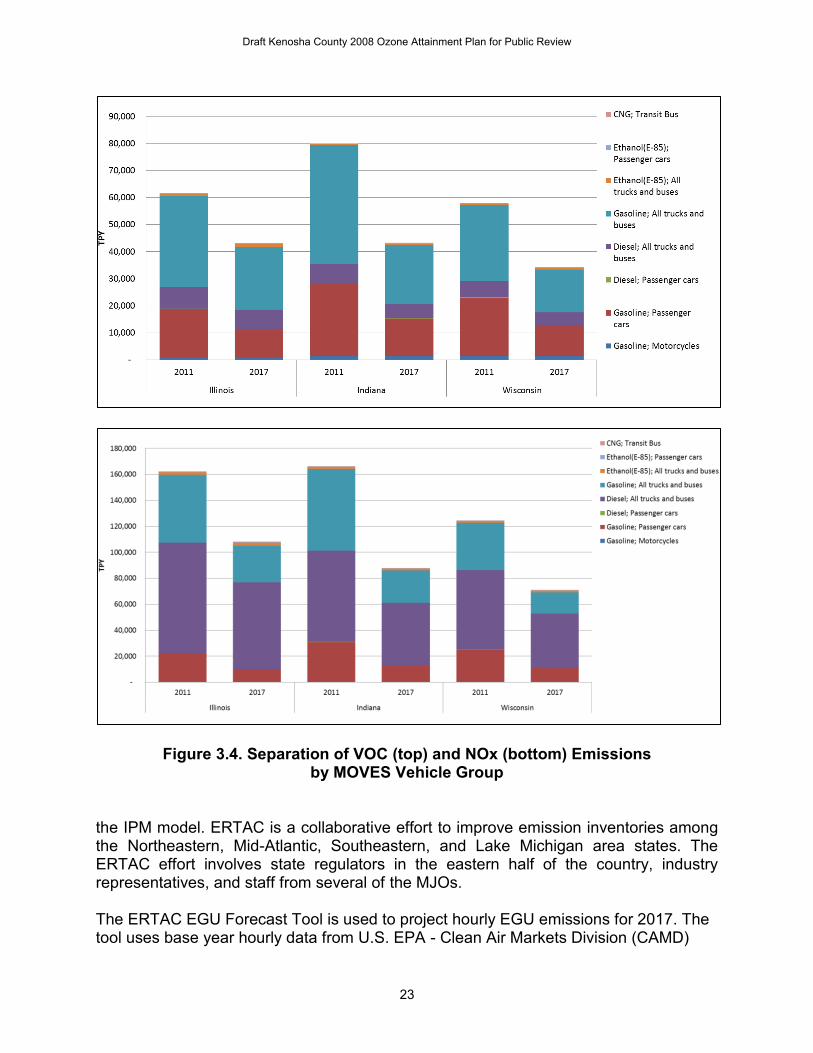
Figure 3.4 illustrates the VOC and NOx emissions contribution from different types of vehicles. As shown in the figure, most VOC emissions from onroad sources, and much of the improvement from 2011 to 2017, are from gasoline powered vehicles. In contrast, NOx emissions are dominated by heavy duty diesel trucks. Gasoline powered vehicles are also significant NOx sources but represent a smaller fraction of the total in future years. Electric Generating Units LADCO used the ERTAC EGU projection tool (version 2.5L2) to develop future year estimates for 2017. EGU emissions were used in place of U.S. EPA’s estimates from
Draft Kenosha County 2008 Ozone Attainment Plan for Public Review
22
Figure 3.2. Base Year (2011) and Future Year (2017)
VOC (top) and NOX (bottom) Emissions (tons per year) for On-Road Mobile Sources
Figure 3.3. VOC Emissions by MOVES Rate Source
Draft Kenosha County 2008 Ozone Attainment Plan for Public Review
23
Figure 3.4. Separation of VOC (top) and NOx (bottom) Emissions by MOVES Vehicle Group
the IPM model. ERTAC is a collaborative effort to improve emission inventories among the Northeastern, Mid-Atlantic, Southeastern, and Lake Michigan area states. The ERTAC effort involves state regulators in the eastern half of the country, industry representatives, and staff from several of the MJOs. The ERTAC EGU Forecast Tool is used to project hourly EGU emissions for 2017. The tool uses base year hourly data from U.S. EPA - Clean Air Markets Division (CAMD)
Draft Kenosha County 2008 Ozone Attainment Plan for Public Review
24
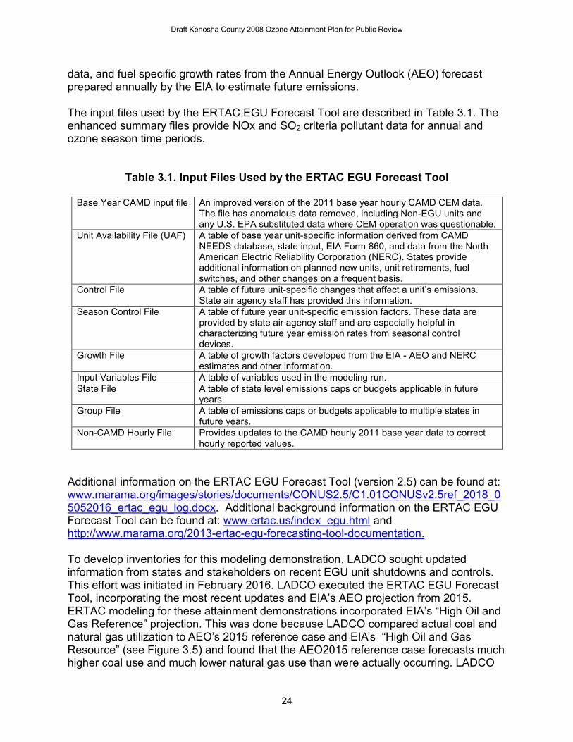
data, and fuel specific growth rates from the Annual Energy Outlook (AEO) forecast prepared annually by the EIA to estimate future emissions. The input files used by the ERTAC EGU Forecast Tool are described in Table 3.1. The enhanced summary files provide NOx and SO2 criteria pollutant data for annual and ozone season time periods.
Table 3.1. Input Files Used by the ERTAC EGU Forecast Tool
Base Year CAMD input file An improved version of the 2011 base year hourly CAMD CEM data. The file has anomalous data removed, including Non-EGU units and any U.S. EPA substituted data where CEM operation was questionable.
Unit Availability File (UAF) A table of base year unit-specific information derived from CAMD NEEDS database, state input, EIA Form 860, and data from the North American Electric Reliability Corporation (NERC). States provide additional information on planned new units, unit retirements, fuel switches, and other changes on a frequent basis.
Control File A table of future unit-specific changes that affect a unit’s emissions. State air agency staff has provided this information.
Season Control File A table of future year unit-specific emission factors. These data are provided by state air agency staff and are especially helpful in characterizing future year emission rates from seasonal control devices.
Growth File A table of growth factors developed from the EIA - AEO and NERC estimates and other information.
Input Variables File A table of variables used in the modeling run. State File A table of state level emissions caps or budgets applicable in future
years. Group File A table of emissions caps or budgets applicable to multiple states in
future years. Non-CAMD Hourly File Provides updates to the CAMD hourly 2011 base year data to correct
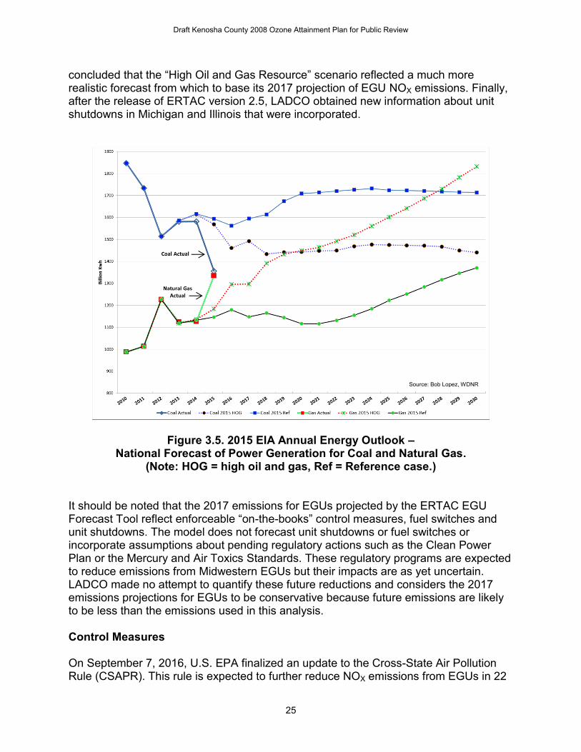
hourly reported values. Additional information on the ERTAC EGU Forecast Tool (version 2.5) can be found at: www.marama.org/images/stories/documents/CONUS2.5/C1.01CONUSv2.5ref_2018_05052016_ertac_egu_log.docx. Additional background information on the ERTAC EGU Forecast Tool can be found at: www.ertac.us/index_egu.html and http://www.marama.org/2013-ertac-egu-forecasting-tool-documentation. To develop inventories for this modeling demonstration, LADCO sought updated information from states and stakeholders on recent EGU unit shutdowns and controls. This effort was initiated in February 2016. LADCO executed the ERTAC EGU Forecast Tool, incorporating the most recent updates and EIA’s AEO projection from 2015. ERTAC modeling for these attainment demonstrations incorporated EIA’s “High Oil and Gas Reference” projection. This was done because LADCO compared actual coal and natural gas utilization to AEO’s 2015 reference case and EIA’s “High Oil and Gas Resource” (see Figure 3.5) and found that the AEO2015 reference case forecasts much higher coal use and much lower natural gas use than were actually occurring. LADCO
Draft Kenosha County 2008 Ozone Attainment Plan for Public Review
25
concluded that the “High Oil and Gas Resource” scenario reflected a much more realistic forecast from which to base its 2017 projection of EGU NOX emissions. Finally, after the release of ERTAC version 2.5, LADCO obtained new information about unit shutdowns in Michigan and Illinois that were incorporated.
Figure 3.5. 2015 EIA Annual Energy Outlook – National Forecast of Power Generation for Coal and Natural Gas.
(Note: HOG = high oil and gas, Ref = Reference case.) It should be noted that the 2017 emissions for EGUs projected by the ERTAC EGU Forecast Tool reflect enforceable “on-the-books” control measures, fuel switches and unit shutdowns. The model does not forecast unit shutdowns or fuel switches or incorporate assumptions about pending regulatory actions such as the Clean Power Plan or the Mercury and Air Toxics Standards. These regulatory programs are expected to reduce emissions from Midwestern EGUs but their impacts are as yet uncertain. LADCO made no attempt to quantify these future reductions and considers the 2017 emissions projections for EGUs to be conservative because future emissions are likely to be less than the emissions used in this analysis. Control Measures On September 7, 2016, U.S. EPA finalized an update to the Cross-State Air Pollution Rule (CSAPR). This rule is expected to further reduce NOX emissions from EGUs in 22
Source: Bob Lopez, WDNR
Draft Kenosha County 2008 Ozone Attainment Plan for Public Review
26
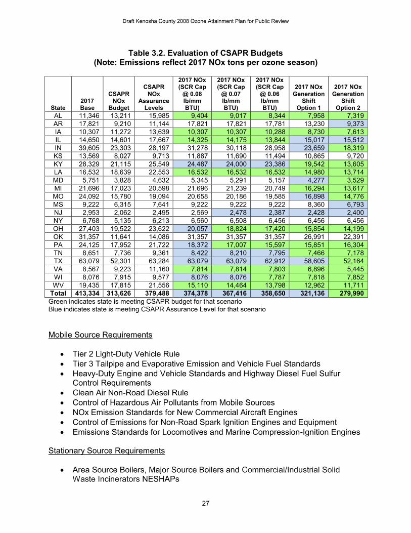
states in the eastern U.S., including five of the states in the LADCO region. These emissions reductions are expected to begin by the start of the 2017 ozone season. LADCO used the ERTAC EGU Forecast Tool to project likely NOx emissions reductions from the revised CSAPR. LADCO’s approach assumed that electric utilities would likely optimize their use of existing controls (SNCRs and SCRs) and shift electric generation from higher emitting units to cleaner ones to comply with CSAPR. LADCO evaluated the likelihood of states meeting the CSAPR ozone season NOx budgets assuming:
lower NOx emission rates for units controlled with SCRs, in the range from 0.06 to 0.08 lb/mm Btu, for SCR-equipped units operating above those rates in the base year;
a lower NOx emission rate for units equipped with SNCRs, to 0.2 lb/mm Btu for SNCR-equipped units operating above that rate in the base year;
electric utilities would shift generation from higher emitting units to cleaner ones, as needed to reduce regional NOx emissions to meet the CSAPR budget.
The results of this analysis are included in Table 3.2. Finding that NOx emissions would exceed the CSAPR NOx budgets for the affected CSAPR region when the most stringent NOx rates for existing equipment were assumed at the baseline loading balance between facilities, LADCO evaluated the effects of shifting electric generation from higher emitting fossil units to lower emitting fossil units. Two such load-shifting scenarios were tested (see Table 3.2). Based on this analysis, it is likely that the CSAPR budget can be achieved in the region using existing controls combined with modest load shifting between fossil-fueled units, assuming meteorological conditions affecting the demand for electricity are similar to base year 2011 conditions. The unit-level emissions resulting from this analysis were used as input to the photochemical air quality model as a future year 2017 control scenario, as described in Section 4 of this TSD. These scenarios were developed based on reasonable assumptions of the likely responses of electric utilities to federal regulatory requirements for the purpose of generating EGU emission rates for this modeling assessment. However, it should be noted that states are required to meet the regulatory requirements of the CSAPR program, not the emissions and generation rates evaluated here. In addition to CSAPR, U.S. EPA has adopted a number of national rules over the past few years that require or will require VOC and NOx emission reductions. Emissions standards established for mobile sources have been phased in over recent years but fleet turnover will ensure continued emissions reductions for many years in the future. For the LADCO states, these rules have provided emissions reductions between 2011 (base year) and 2017 (attainment year), and have been factored into the modeling assessment. The national rules that will help states achieve the 2008 ozone NAAQS are listed below.
Draft Kenosha County 2008 Ozone Attainment Plan for Public Review
27
Table 3.2. Evaluation of CSAPR Budgets (Note: Emissions reflect 2017 NOx tons per ozone season)
State 2017 Base
CSAPR NOx
Budget
CSAPR NOx
Assurance Levels
2017 NOx (SCR Cap
@ 0.08 lb/mm BTU)
2017 NOx (SCR Cap
@ 0.07 lb/mm BTU)
2017 NOx (SCR Cap
@ 0.06 lb/mm BTU)
2017 NOx Generation
Shift Option 1
2017 NOx Generation
Shift Option 2
AL 11,346 13,211 15,985 9,404 9,017 8,344 7,958 7,319 AR 17,821 9,210 11,144 17,821 17,821 17,781 13,230 9,373 IA 10,307 11,272 13,639 10,307 10,307 10,288 8,730 7,613 IL 14,650 14,601 17,667 14,325 14,175 13,844 15,017 15,512 IN 39,605 23,303 28,197 31,278 30,118 28,958 23,659 18,319 KS 13,569 8,027 9,713 11,887 11,690 11,494 10,865 9,720 KY 28,329 21,115 25,549 24,487 24,000 23,386 19,542 13,605 LA 16,532 18,639 22,553 16,532 16,532 16,532 14,980 13,714 MD 5,751 3,828 4,632 5,345 5,291 5,157 4,277 3,529 MI 21,696 17,023 20,598 21,696 21,239 20,749 16,294 13,617 MO 24,092 15,780 19,094 20,658 20,186 19,585 16,898 14,776 MS 9,222 6,315 7,641 9,222 9,222 9,222 8,360 6,793 NJ 2,953 2,062 2,495 2,569 2,478 2,387 2,428 2,400 NY 6,768 5,135 6,213 6,560 6,508 6,456 6,456 6,456 OH 27,403 19,522 23,622 20,057 18,824 17,420 15,854 14,199 OK 31,357 11,641 14,086 31,357 31,357 31,357 26,991 22,391 PA 24,125 17,952 21,722 18,372 17,007 15,597 15,851 16,304 TN 8,651 7,736 9,361 8,422 8,210 7,795 7,466 7,178 TX 63,079 52,301 63,284 63,079 63,079 62,912 58,605 52,164 VA 8,567 9,223 11,160 7,814 7,814 7,803 6,896 5,445 WI 8,076 7,915 9,577 8,076 8,076 7,787 7,818 7,852 WV 19,435 17,815 21,556 15,110 14,464 13,798 12,962 11,711
Total 413,334 313,626 379,488 374,378 367,416 358,650 321,136 279,990 Green indicates state is meeting CSAPR budget for that scenario Blue indicates state is meeting CSAPR Assurance Level for that scenario Mobile Source Requirements
Tier 2 Light-Duty Vehicle Rule Tier 3 Tailpipe and Evaporative Emission and Vehicle Fuel Standards Heavy-Duty Engine and Vehicle Standards and Highway Diesel Fuel Sulfur
Control Requirements Clean Air Non-Road Diesel Rule Control of Hazardous Air Pollutants from Mobile Sources NOx Emission Standards for New Commercial Aircraft Engines Control of Emissions for Non-Road Spark Ignition Engines and Equipment Emissions Standards for Locomotives and Marine Compression-Ignition Engines
Stationary Source Requirements
Area Source Boilers, Major Source Boilers and Commercial/Industrial Solid Waste Incinerators NESHAPs
Draft Kenosha County 2008 Ozone Attainment Plan for Public Review
28
Reciprocating Internal Combustion Engines NESHAPs Mercury and Air Toxics Standards (Note that this modeling demonstration
includes reductions from this rule as implemented by early 2016 when modeling was initiated. Further emissions reductions are expected from that have not been accounted for in this analysis.)
Regional Haze Regulations and Guidelines for Best Available Retrofit Technology
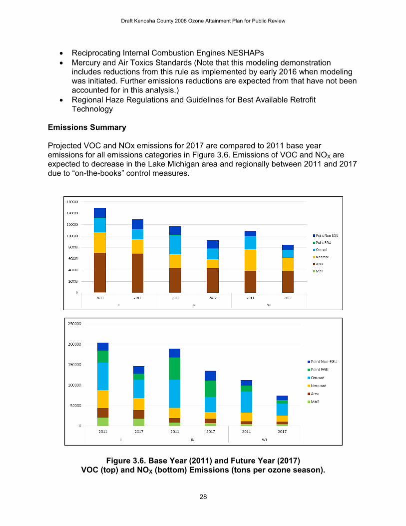
Emissions Summary Projected VOC and NOx emissions for 2017 are compared to 2011 base year emissions for all emissions categories in Figure 3.6. Emissions of VOC and NOX are expected to decrease in the Lake Michigan area and regionally between 2011 and 2017 due to “on-the-books” control measures.
Figure 3.6. Base Year (2011) and Future Year (2017) VOC (top) and NOX (bottom) Emissions (tons per ozone season).
Draft Kenosha County 2008 Ozone Attainment Plan for Public Review
29
4.0 Air Quality Modeling This section reviews the development and evaluation of the modeling system used for the Chicago and Sheboygan ozone attainment test. LADCO, in cooperation with the Illinois EPA, the Indiana DEM, the Wisconsin DNR and U.S. EPA, conducted the modeling assessment described here to support the development of the states’ ozone attainment SIPs. The modeling analyses were conducted in accordance with U.S. EPA’s attainment demonstration guidelines (U.S. EPA, 2014B). Selection of Base Year The calendar year 2011 was selected as the base year for regional ozone modeling, based on the following considerations:
The 2011 base year is representative of the observed baseline design values for the time period (2008-2010 and 2009-2011) when U.S. EPA established the final air quality designations for the Sheboygan and Chicago areas for the 2008 ozone NAAQS, respectively.
There are extensive air quality, meteorological, and emissions databases that have been developed for 2011 by U.S. EPA, and others, for regulatory purposes (U.S. EPA, 2015A).
The 2011 ozone season was fairly typical in terms of meteorology and ozone conduciveness in the Lake Michigan region.
Modeling Platform The modeling platform consists of emissions and transport models that reflect the spatial and temporal characteristics of the study region. U.S. EPA’s modeling guidance details several prerequisites for a model to be used to support an attainment demonstration:
It should have received a scientific peer review; It should be appropriate for the specific application on a theoretical basis; It should be used with databases that are available and adequate to
support its application; and It should be shown to have performed well in past modeling applications.
A summary of the models used in the 2011 modeling platform are shown in Table 4.1.
Table 4.1. 2011 Modeling Platform Components Model Type Managing Organization WRF Meteorology EPA OAQPS GEOS-CHEM Global Chemical Transport EPA OAQPS SMOKE Emissions EPA OAQPS / LADCO ERTAC EGU emissions States, MJOs CAMx Regional Photochemical LADCO
Draft Kenosha County 2008 Ozone Attainment Plan for Public Review
30
Below is a brief summary of each of the model components:
WRF: The Weather Research and Forecasting (WRF) model was developed collaboratively by the National Center for Atmospheric Research, the National Oceanic and Atmospheric Administration, the Department of Defense’s Air Force Weather Agency and Naval Research Laboratory, the Center for Analysis and Prediction of Storms at the University of Oklahoma, and the Federal Aviation Administration, with the participation of university scientists. WRF is a prognostic meteorological model routinely used by U.S. EPA and others for urban- and regional-scale photochemical modeling of PM2.5, ozone, and regional haze (U.S. EPA, 2014A).
GEOS-CHEM: Bey et al. (2001) developed the global chemical transport model GEOS-Chem using assimilated meteorological data from the Goddard Earth Observing System (GEOS) of the NASA Global Modeling and Assimilation Office. The model incorporates modules to account for emissions, photochemistry, and deposition. GEOS-Chem is managed by Harvard University and Dalhousie University with support from the U.S. NASA Earth Science Division and the Canadian National and Engineering Research Council.
SMOKE: The SMOKE modeling system is an emissions modeling system that generates hourly gridded, speciated emission inputs of mobile, nonroad, area, point, fire and biogenic emission sources for photochemical grid models. Its purpose is to provide an efficient tool for converting emissions inventory data into the formatted emission files required by an air quality simulation model. For mobile sources, SMOKE actually generates emissions rates based on input mobile-source activity data, using emission factors and outputs from U.S. EPA’s MOVES mobile-source emissions model. For EGUs, SMOKE generates hourly emissions based on hourly outputs from the ERTAC EGU Forecast Tool, described below.
ERTAC: ERTAC is a collaborative effort to improve emission inventories among the Northeastern, Mid-Atlantic, Southeastern, and Lake Michigan area states; other member states; industry representatives; and MJOs. ERTAC developed the EGU Forecast Tool for states to use for SIP planning. The tool uses base-year reported EGU data obtained from CAMD and applies growth rates by region and fuel type provided by the EIA to estimate future emissions. The ERTAC EGU Forecast Tool is open-source and has been provided to U.S. EPA.
CAMx: CAMx is a photochemical grid model that is designed for simulating atmospheric transport and chemical transformation of air pollution over urban to regional scales. CAMx is a state-of-the-science open-source air quality model that is computationally efficient with an extensive history of regulatory applications. The selection of CAMx as the primary photochemical grid model is
Draft Kenosha County 2008 Ozone Attainment Plan for Public Review
31
based on several factors including performance, operational considerations (e.g., ease of application and resource requirements), technical support and documentation, and model extensions (e.g., process analysis, source apportionment, and plume-in-grid).
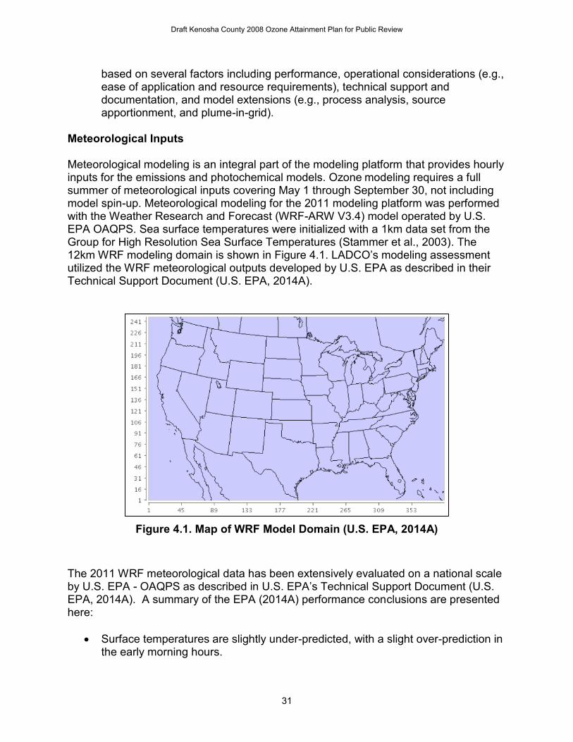
Meteorological Inputs Meteorological modeling is an integral part of the modeling platform that provides hourly inputs for the emissions and photochemical models. Ozone modeling requires a full summer of meteorological inputs covering May 1 through September 30, not including model spin-up. Meteorological modeling for the 2011 modeling platform was performed with the Weather Research and Forecast (WRF-ARW V3.4) model operated by U.S. EPA OAQPS. Sea surface temperatures were initialized with a 1km data set from the Group for High Resolution Sea Surface Temperatures (Stammer et al., 2003). The 12km WRF modeling domain is shown in Figure 4.1. LADCO’s modeling assessment utilized the WRF meteorological outputs developed by U.S. EPA as described in their Technical Support Document (U.S. EPA, 2014A).
Figure 4.1. Map of WRF Model Domain (U.S. EPA, 2014A)
The 2011 WRF meteorological data has been extensively evaluated on a national scale by U.S. EPA - OAQPS as described in U.S. EPA’s Technical Support Document (U.S. EPA, 2014A). A summary of the EPA (2014A) performance conclusions are presented here:
Surface temperatures are slightly under-predicted, with a slight over-prediction in the early morning hours.
Draft Kenosha County 2008 Ozone Attainment Plan for Public Review
32
Wind speeds are slightly over-predicted in the early morning and slightly under-predicted in the evening and night.
Mixing ratios are generally under-predicted in the central and western US and over-predicted in the eastern states.
Precipitation is overestimated in elevated terrain such as northern CA and the Pacific Northwest.
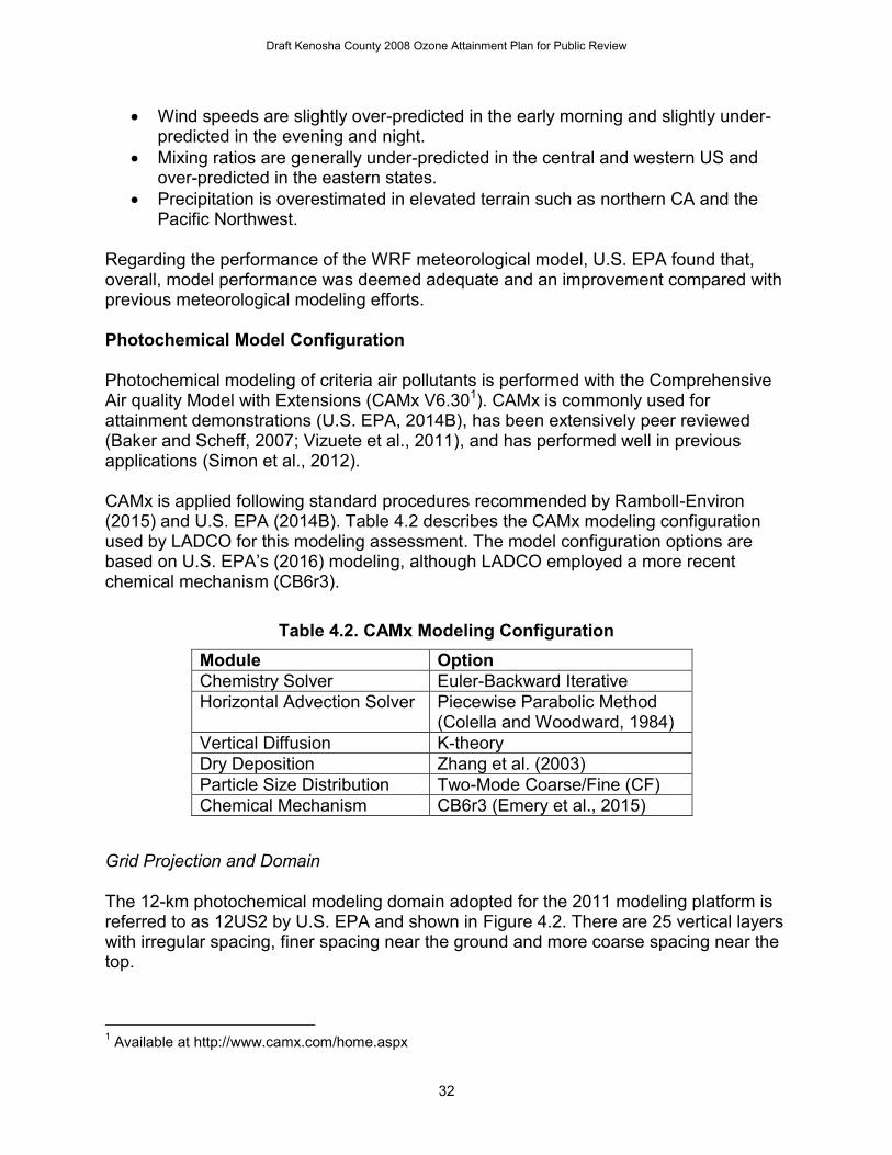
Regarding the performance of the WRF meteorological model, U.S. EPA found that, overall, model performance was deemed adequate and an improvement compared with previous meteorological modeling efforts. Photochemical Model Configuration Photochemical modeling of criteria air pollutants is performed with the Comprehensive Air quality Model with Extensions (CAMx V6.301). CAMx is commonly used for attainment demonstrations (U.S. EPA, 2014B), has been extensively peer reviewed (Baker and Scheff, 2007; Vizuete et al., 2011), and has performed well in previous applications (Simon et al., 2012). CAMx is applied following standard procedures recommended by Ramboll-Environ (2015) and U.S. EPA (2014B). Table 4.2 describes the CAMx modeling configuration used by LADCO for this modeling assessment. The model configuration options are based on U.S. EPA’s (2016) modeling, although LADCO employed a more recent chemical mechanism (CB6r3).
Table 4.2. CAMx Modeling Configuration Module Option Chemistry Solver Euler-Backward Iterative Horizontal Advection Solver Piecewise Parabolic Method
(Colella and Woodward, 1984) Vertical Diffusion K-theory Dry Deposition Zhang et al. (2003) Particle Size Distribution Two-Mode Coarse/Fine (CF) Chemical Mechanism CB6r3 (Emery et al., 2015)
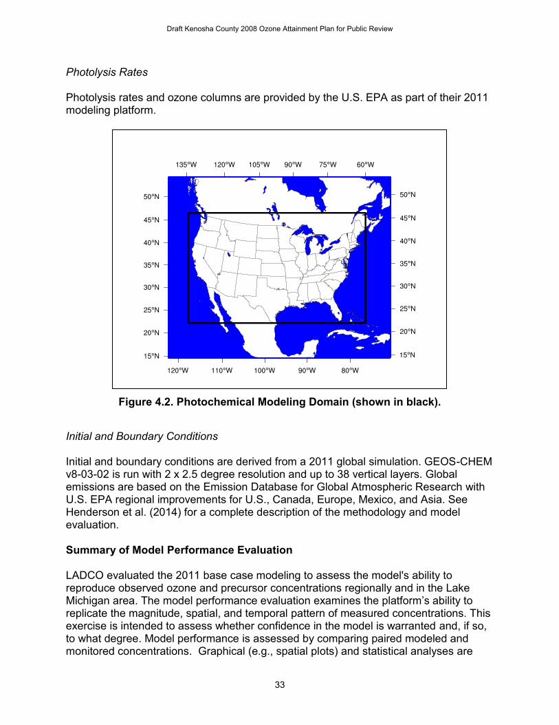
Grid Projection and Domain The 12-km photochemical modeling domain adopted for the 2011 modeling platform is referred to as 12US2 by U.S. EPA and shown in Figure 4.2. There are 25 vertical layers with irregular spacing, finer spacing near the ground and more coarse spacing near the top.
1 Available at http://www.camx.com/home.aspx
Draft Kenosha County 2008 Ozone Attainment Plan for Public Review
33
Photolysis Rates Photolysis rates and ozone columns are provided by the U.S. EPA as part of their 2011 modeling platform.
Figure 4.2. Photochemical Modeling Domain (shown in black).
Initial and Boundary Conditions Initial and boundary conditions are derived from a 2011 global simulation. GEOS-CHEM v8-03-02 is run with 2 x 2.5 degree resolution and up to 38 vertical layers. Global emissions are based on the Emission Database for Global Atmospheric Research with U.S. EPA regional improvements for U.S., Canada, Europe, Mexico, and Asia. See Henderson et al. (2014) for a complete description of the methodology and model evaluation. Summary of Model Performance Evaluation LADCO evaluated the 2011 base case modeling to assess the model's ability to reproduce observed ozone and precursor concentrations regionally and in the Lake Michigan area. The model performance evaluation examines the platform’s ability to replicate the magnitude, spatial, and temporal pattern of measured concentrations. This exercise is intended to assess whether confidence in the model is warranted and, if so, to what degree. Model performance is assessed by comparing paired modeled and monitored concentrations. Graphical (e.g., spatial plots) and statistical analyses are
Draft Kenosha County 2008 Ozone Attainment Plan for Public Review
34
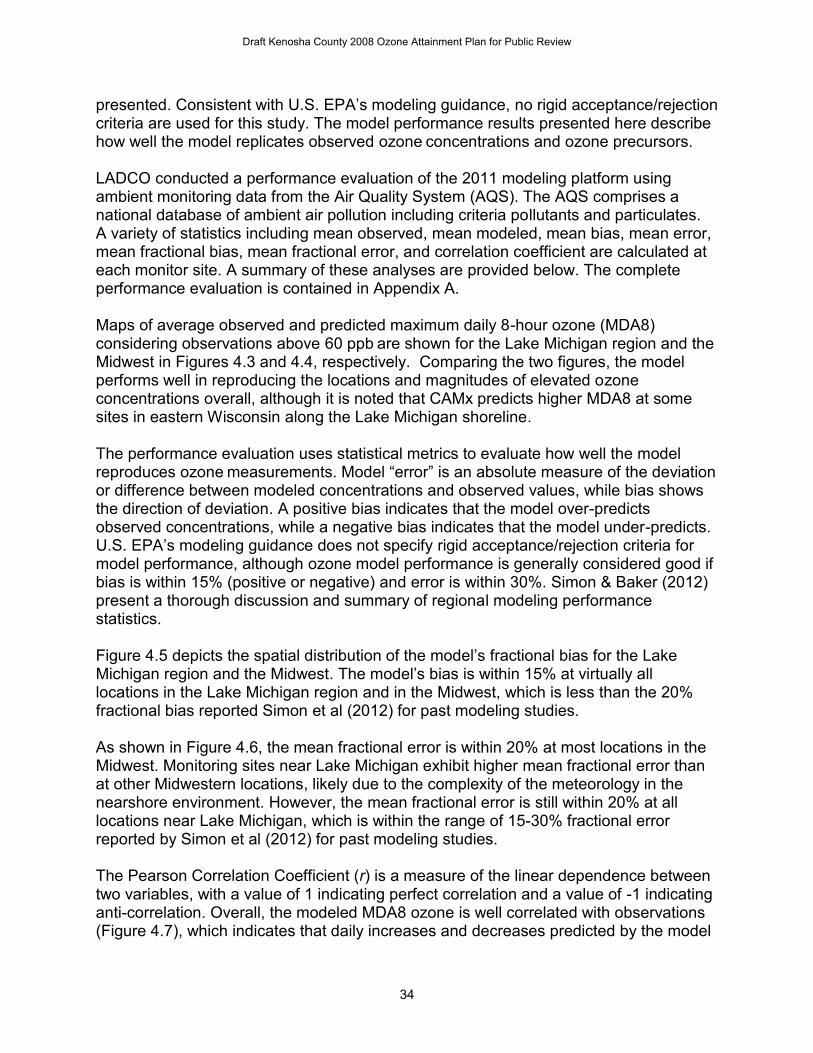
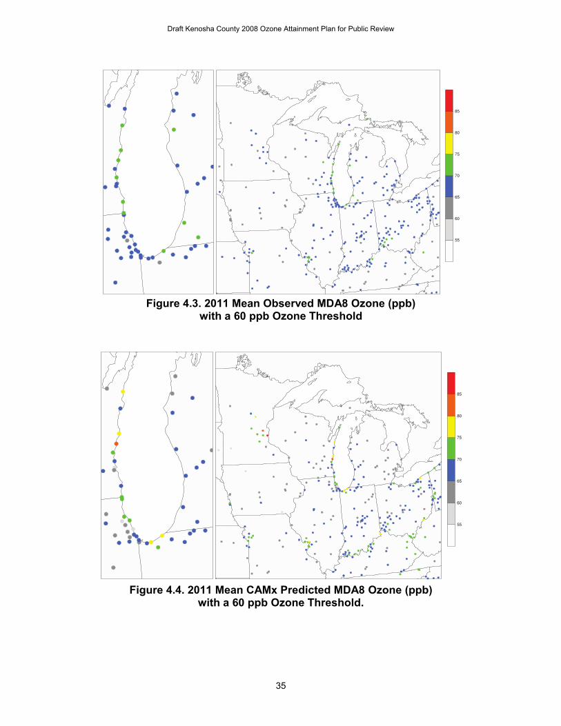
presented. Consistent with U.S. EPA’s modeling guidance, no rigid acceptance/rejection criteria are used for this study. The model performance results presented here describe how well the model replicates observed ozone concentrations and ozone precursors. LADCO conducted a performance evaluation of the 2011 modeling platform using ambient monitoring data from the Air Quality System (AQS). The AQS comprises a national database of ambient air pollution including criteria pollutants and particulates. A variety of statistics including mean observed, mean modeled, mean bias, mean error, mean fractional bias, mean fractional error, and correlation coefficient are calculated at each monitor site. A summary of these analyses are provided below. The complete performance evaluation is contained in Appendix A. Maps of average observed and predicted maximum daily 8-hour ozone (MDA8) considering observations above 60 ppb are shown for the Lake Michigan region and the Midwest in Figures 4.3 and 4.4, respectively. Comparing the two figures, the model performs well in reproducing the locations and magnitudes of elevated ozone
concentrations overall, although it is noted that CAMx predicts higher MDA8 at some sites in eastern Wisconsin along the Lake Michigan shoreline. The performance evaluation uses statistical metrics to evaluate how well the model reproduces ozone measurements. Model “error” is an absolute measure of the deviation or difference between modeled concentrations and observed values, while bias shows the direction of deviation. A positive bias indicates that the model over-predicts observed concentrations, while a negative bias indicates that the model under-predicts. U.S. EPA’s modeling guidance does not specify rigid acceptance/rejection criteria for model performance, although ozone model performance is generally considered good if bias is within 15% (positive or negative) and error is within 30%. Simon & Baker (2012) present a thorough discussion and summary of regional modeling performance statistics. Figure 4.5 depicts the spatial distribution of the model’s fractional bias for the Lake Michigan region and the Midwest. The model’s bias is within 15% at virtually all locations in the Lake Michigan region and in the Midwest, which is less than the 20% fractional bias reported Simon et al (2012) for past modeling studies. As shown in Figure 4.6, the mean fractional error is within 20% at most locations in the Midwest. Monitoring sites near Lake Michigan exhibit higher mean fractional error than at other Midwestern locations, likely due to the complexity of the meteorology in the nearshore environment. However, the mean fractional error is still within 20% at all locations near Lake Michigan, which is within the range of 15-30% fractional error reported by Simon et al (2012) for past modeling studies. The Pearson Correlation Coefficient (r) is a measure of the linear dependence between two variables, with a value of 1 indicating perfect correlation and a value of -1 indicating anti-correlation. Overall, the modeled MDA8 ozone is well correlated with observations (Figure 4.7), which indicates that daily increases and decreases predicted by the model
Draft Kenosha County 2008 Ozone Attainment Plan for Public Review
35
Figure 4.3. 2011 Mean Observed MDA8 Ozone (ppb)
with a 60 ppb Ozone Threshold
Figure 4.4. 2011 Mean CAMx Predicted MDA8 Ozone (ppb)
with a 60 ppb Ozone Threshold.
Draft Kenosha County 2008 Ozone Attainment Plan for Public Review
36
Figure 4.5. 2011 Mean Fractional Bias of MDA8 Ozone (ppb)
with a 60 ppb Ozone Threshold
Figure 4.6. 2011 Mean Fractional Error of MDA8 Ozone (ppb)
with a 60 ppb Ozone Threshold
Draft Kenosha County 2008 Ozone Attainment Plan for Public Review
37
Figure 4.7. 2011 Pearson Correlation Coefficient of MDA8 Ozone (ppb) with a 60 ppb Ozone Threshold
track well with observations. Not all monitors are well correlated with modeling results; some monitors exhibit a low or even negative correlation. The model is not expected to perform perfectly at every individual monitor. Simon et al (2012) reported values ranging from 0.2 to 0.75 for MDA8 ozone. One easy way to summarize model performance and compare it to the performance goals is through the use of box plots. Box plots summarizing fractional error and fractional bias aggregated by month are shown in Figures 4.8 and 4.9 for the LADCO states and selected cities in the LADCO region, respectively. The dotted lines show performance criteria goals defined from ranges of performance statistics reported by Simon et al (2012). Generally, the modeling results fall within the performance goals, since the model’s bias is less than 10% and the model’s mean error is less than 20% for most areas. Some sites exhibit strongly positive or negative bias during the months of May and September when there are fewer ozone episodes. The performance of the model in LADCO states is similar to national model performance, although the model tends to have a slightly negative bias predicting MDA8 ozone. This finding is consistent with past modeling studies (Simon et al, 2012). Focusing on the lakeshore nonattainment sites, time series of modeled and monitored MDA8 ozone for the 2011 ozone season are shown in Figures 4.10 and 4.11 for the monitors at Chiwaukee Prairie and Sheboygan. The modeled values for MDA8 ozone are of similar magnitudes as the measured values and follow temporal variations well. While the model generally under-predicts MDA8 ozone, as described above, the
Draft Kenosha County 2008 Ozone Attainment Plan for Public Review
38
Figure 4.8. MDA8 Ozone Model Performance by Month for the LADCO States,
LADCO Aggregated (purple), and National Average (black)
Figure 4.9. MDA8 Ozone Model Performance for Selected Cities
in the LADCO Region
Draft Kenosha County 2008 Ozone Attainment Plan for Public Review
39
Figure 4.10. MDA8 Ozone Showing Monitoring and Modeling
in Chiwaukee Prairie, WI (AQS site ID 550590019)
Figure 4.11. Time Series Comparing Observed and Predicted
MDA8 Ozone in Sheboygan, WI (AQS site ID 551170006) Sheboygan and Chiwaukee monitors exhibit a slight over-prediction of MDA8 ozone as shown in Figures 4.10 and 4.11, respectively. As discussed, U.S. EPA’s modeling guidance does not specify rigid acceptance/rejection criteria for model performance, although ozone model performance is generally considered good if bias is within 15% (positive or negative), error is within 30%. The performance of the 2011 modeling platform meets these metrics, both in the Lake Michigan area and in the wider region. This modeling is an improvement over past modeling studies (Simon et al, 2012) and is acceptable for supporting the states’ attainment SIPs. Modeled Attainment Test An attainment demonstration based on air quality modeling is used to determine whether identified emissions reduction measures are sufficient to reduce projected pollutant concentrations to a level that meets the NAAQS by the statutory deadline
Draft Kenosha County 2008 Ozone Attainment Plan for Public Review
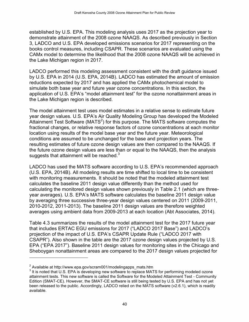
40
established by U.S. EPA. This modeling analysis uses 2017 as the projection year to demonstrate attainment of the 2008 ozone NAAQS. As described previously in Section 3, LADCO and U.S. EPA developed emissions scenarios for 2017 representing on the books control measures, including CSAPR. These scenarios are evaluated using the CAMx model to determine the likelihood that the 2008 ozone NAAQS will be achieved in the Lake Michigan region in 2017. LADCO performed this modeling assessment consistent with the draft guidance issued by U.S. EPA in 2014 (U.S. EPA, 2014B). LADCO has estimated the amount of emission reductions expected by 2017 and has applied the CAMx photochemical model to simulate both base year and future year ozone concentrations. In this section, the application of U.S. EPA’s “model attainment test” for the ozone nonattainment areas in the Lake Michigan region is described. The model attainment test uses model estimates in a relative sense to estimate future year design values. U.S. EPA’s Air Quality Modeling Group has developed the Modeled Attainment Test Software (MATS2) for this purpose. The MATS software computes the fractional changes, or relative response factors of ozone concentrations at each monitor location using results of the model base year and the future year. Meteorological conditions are assumed to be unchanged for the base and projection years. The resulting estimates of future ozone design values are then compared to the NAAQS. If the future ozone design values are less than or equal to the NAAQS, then the analysis suggests that attainment will be reached.3 LADCO has used the MATS software according to U.S. EPA’s recommended approach (U.S. EPA, 2014B). All modeling results are time shifted to local time to be consistent with monitoring measurements. It should be noted that the modeled attainment test calculates the baseline 2011 design value differently than the method used for calculating the monitored design values shown previously in Table 2.1 (which are three-year averages). U.S. EPA’s MATS software calculates the baseline 2011 design value by averaging three successive three-year design values centered on 2011 (2009-2011, 2010-2012, 2011-2013). The baseline 2011 design values are therefore weighted averages using ambient data from 2009-2013 at each location (Abt Associates, 2014). Table 4.3 summarizes the results of the model attainment test for the 2017 future year that includes ERTAC EGU emissions for 2017 (“LADCO 2017 Base”) and LADCO’s projection of the impact of U.S. EPA’s CSAPR Update Rule (“LADCO 2017 with CSAPR”). Also shown in the table are the 2017 ozone design values projected by U.S. EPA (“EPA 2017”). Baseline 2011 design values for monitoring sites in the Chicago and Sheboygan nonattainment areas are compared to the 2017 design values projected for 2 Available at http://www.epa.gov/scram001/modelingapps_mats.htm 3 It is noted that U.S. EPA is developing new software to replace MATS for performing modeled ozone attainment tests. This new software is called the Software for the Modeled Attainment Test - Community Edition (SMAT-CE). However, the SMAT-CE software is still being tested by U.S. EPA and has not yet been released to the public. Accordingly, LADCO relied on the MATS software (v2.6.1), which is readily available.
Draft Kenosha County 2008 Ozone Attainment Plan for Public Review
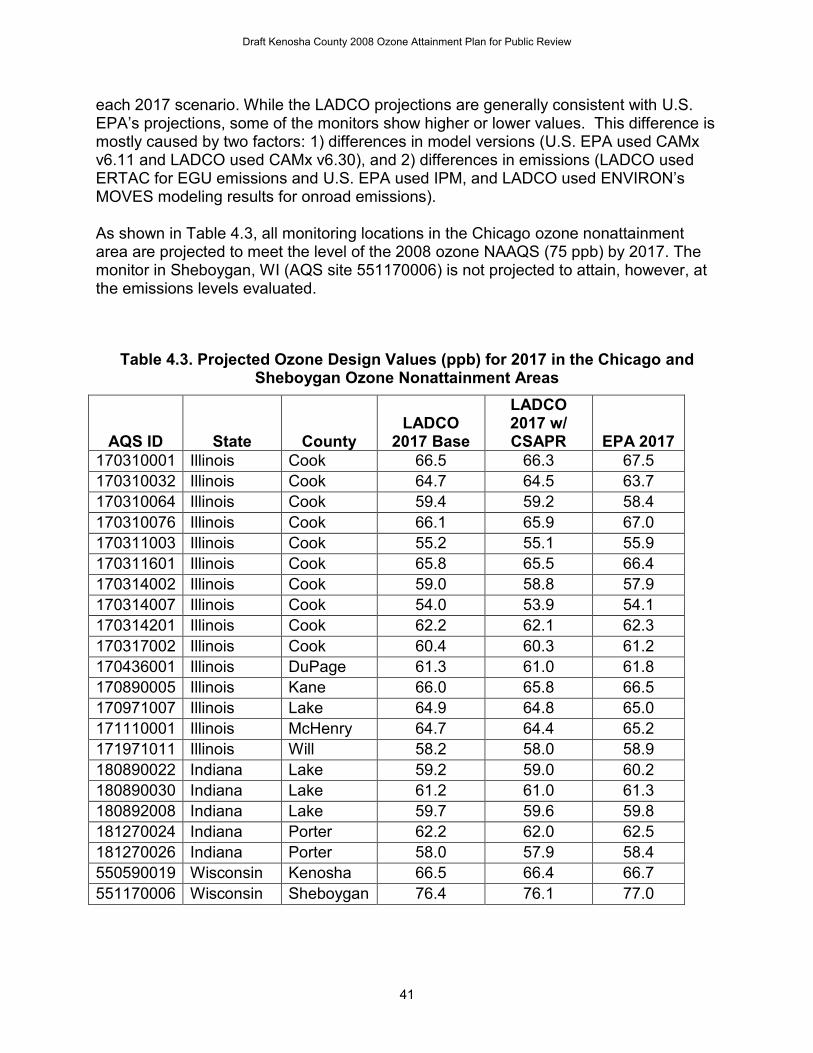
41
each 2017 scenario. While the LADCO projections are generally consistent with U.S. EPA’s projections, some of the monitors show higher or lower values. This difference is mostly caused by two factors: 1) differences in model versions (U.S. EPA used CAMx v6.11 and LADCO used CAMx v6.30), and 2) differences in emissions (LADCO used ERTAC for EGU emissions and U.S. EPA used IPM, and LADCO used ENVIRON’s MOVES modeling results for onroad emissions). As shown in Table 4.3, all monitoring locations in the Chicago ozone nonattainment area are projected to meet the level of the 2008 ozone NAAQS (75 ppb) by 2017. The monitor in Sheboygan, WI (AQS site 551170006) is not projected to attain, however, at the emissions levels evaluated.
Table 4.3. Projected Ozone Design Values (ppb) for 2017 in the Chicago and
Sheboygan Ozone Nonattainment Areas
AQS ID State County LADCO
2017 Base
LADCO 2017 w/ CSAPR EPA 2017
170310001 Illinois Cook 66.5 66.3 67.5 170310032 Illinois Cook 64.7 64.5 63.7 170310064 Illinois Cook 59.4 59.2 58.4 170310076 Illinois Cook 66.1 65.9 67.0 170311003 Illinois Cook 55.2 55.1 55.9 170311601 Illinois Cook 65.8 65.5 66.4 170314002 Illinois Cook 59.0 58.8 57.9 170314007 Illinois Cook 54.0 53.9 54.1 170314201 Illinois Cook 62.2 62.1 62.3 170317002 Illinois Cook 60.4 60.3 61.2 170436001 Illinois DuPage 61.3 61.0 61.8 170890005 Illinois Kane 66.0 65.8 66.5 170971007 Illinois Lake 64.9 64.8 65.0 171110001 Illinois McHenry 64.7 64.4 65.2 171971011 Illinois Will 58.2 58.0 58.9 180890022 Indiana Lake 59.2 59.0 60.2 180890030 Indiana Lake 61.2 61.0 61.3 180892008 Indiana Lake 59.7 59.6 59.8 181270024 Indiana Porter 62.2 62.0 62.5 181270026 Indiana Porter 58.0 57.9 58.4 550590019 Wisconsin Kenosha 66.5 66.4 66.7 551170006 Wisconsin Sheboygan 76.4 76.1 77.0
Draft Kenosha County 2008 Ozone Attainment Plan for Public Review
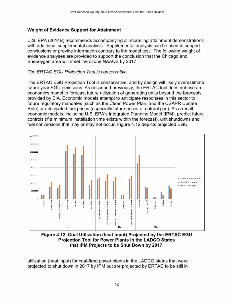
42
Weight of Evidence Support for Attainment U.S. EPA (2014B) recommends accompanying all modeling attainment demonstrations with additional supplemental analysis. Supplemental analysis can be used to support conclusions or provide information contrary to the model test. The following weight of evidence analyses are provided to support the conclusion that the Chicago and Sheboygan area will meet the ozone NAAQS by 2017. The ERTAC EGU Projection Tool is conservative The ERTAC EGU Projection Tool is conservative, and by design will likely overestimate future year EGU emissions. As described previously, the ERTAC tool does not use an economics model to forecast future utilization of generating units beyond the forecasts provided by EIA. Economic models attempt to anticipate responses in this sector to future regulatory mandates (such as the Clean Power Plan, and the CSAPR Update Rule) or anticipated fuel prices (especially future prices of natural gas). As a result, economic models, including U.S. EPA’s Integrated Planning Model (IPM), predict future controls (if a minimum installation time exists within the forecast), unit shutdowns and fuel conversions that may or may not occur. Figure 4.12 depicts projected EGU
Figure 4.12. Coal Utilization (heat input) Projected by the ERTAC EGU
Projection Tool for Power Plants in the LADCO States that IPM Projects to be Shut Down by 2017.
utilization (heat input) for coal-fired power plants in the LADCO states that were projected to shut down in 2017 by IPM but are projected by ERTAC to be still in
Draft Kenosha County 2008 Ozone Attainment Plan for Public Review
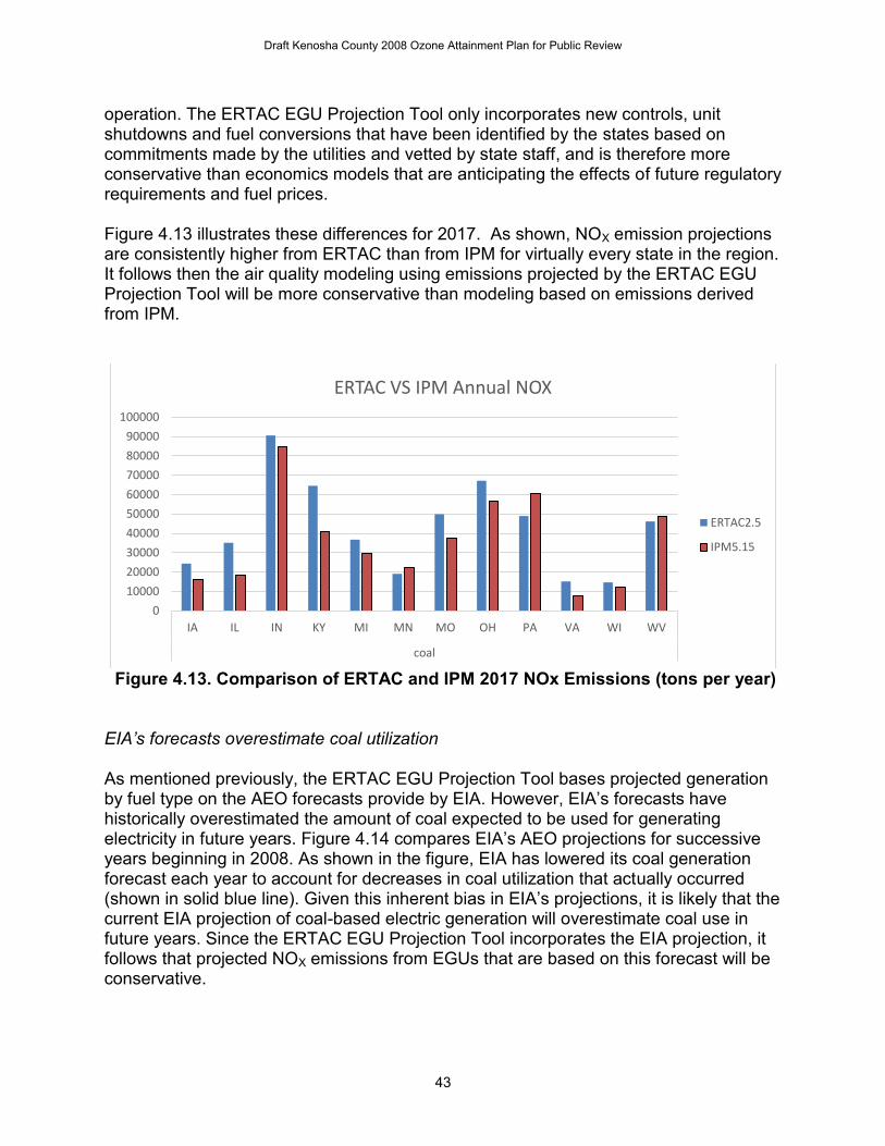
43
operation. The ERTAC EGU Projection Tool only incorporates new controls, unit shutdowns and fuel conversions that have been identified by the states based on commitments made by the utilities and vetted by state staff, and is therefore more conservative than economics models that are anticipating the effects of future regulatory requirements and fuel prices. Figure 4.13 illustrates these differences for 2017. As shown, NOX emission projections are consistently higher from ERTAC than from IPM for virtually every state in the region. It follows then the air quality modeling using emissions projected by the ERTAC EGU Projection Tool will be more conservative than modeling based on emissions derived from IPM.
Figure 4.13. Comparison of ERTAC and IPM 2017 NOx Emissions (tons per year)
EIA’s forecasts overestimate coal utilization As mentioned previously, the ERTAC EGU Projection Tool bases projected generation by fuel type on the AEO forecasts provide by EIA. However, EIA’s forecasts have historically overestimated the amount of coal expected to be used for generating electricity in future years. Figure 4.14 compares EIA’s AEO projections for successive years beginning in 2008. As shown in the figure, EIA has lowered its coal generation forecast each year to account for decreases in coal utilization that actually occurred (shown in solid blue line). Given this inherent bias in EIA’s projections, it is likely that the current EIA projection of coal-based electric generation will overestimate coal use in future years. Since the ERTAC EGU Projection Tool incorporates the EIA projection, it follows that projected NOX emissions from EGUs that are based on this forecast will be conservative.
0
10000
20000
30000
40000
50000
60000
70000
80000
90000
100000
IA IL IN KY MI MN MO OH PA VA WI WV
coal
ERTAC VS IPM Annual NOX
ERTAC2.5
IPM5.15
Draft Kenosha County 2008 Ozone Attainment Plan for Public Review
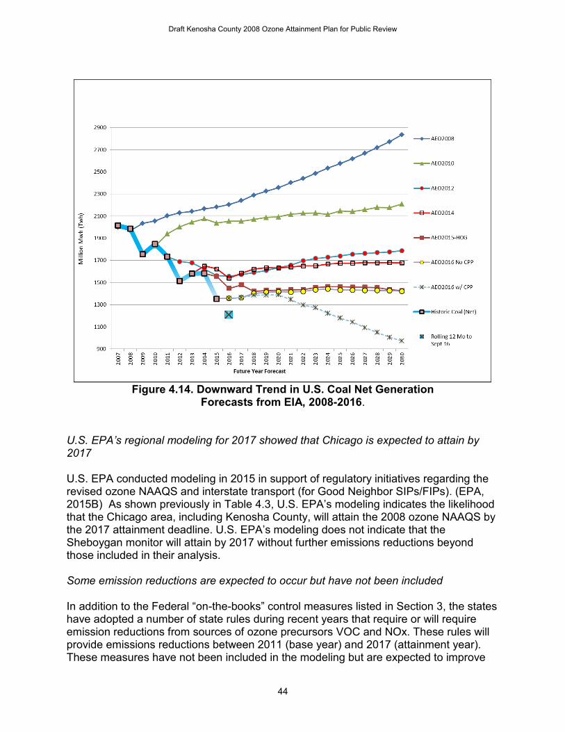
44
Figure 4.14. Downward Trend in U.S. Coal Net Generation
Forecasts from EIA, 2008-2016. U.S. EPA’s regional modeling for 2017 showed that Chicago is expected to attain by 2017 U.S. EPA conducted modeling in 2015 in support of regulatory initiatives regarding the revised ozone NAAQS and interstate transport (for Good Neighbor SIPs/FIPs). (EPA, 2015B) As shown previously in Table 4.3, U.S. EPA’s modeling indicates the likelihood that the Chicago area, including Kenosha County, will attain the 2008 ozone NAAQS by the 2017 attainment deadline. U.S. EPA’s modeling does not indicate that the Sheboygan monitor will attain by 2017 without further emissions reductions beyond those included in their analysis. Some emission reductions are expected to occur but have not been included In addition to the Federal “on-the-books” control measures listed in Section 3, the states have adopted a number of state rules during recent years that require or will require emission reductions from sources of ozone precursors VOC and NOx. These rules will provide emissions reductions between 2011 (base year) and 2017 (attainment year). These measures have not been included in the modeling but are expected to improve
Draft Kenosha County 2008 Ozone Attainment Plan for Public Review
45
ozone air quality in Chicago and Sheboygan. Such measures include:
Consumer products and AIM requirements in Illinois and Indiana Stage II removal and low permeable hose requirements Certain shutdowns and restrictions that have occurred since development of the
attainment modeling Illinois’ NOx regulations for ozone nonattainment areas
Alternate MATS Inputs Yield Range of Future Year Design Values LADCO has used the MATS software according to U.S. EPA’s recommended approach (U.S. EPA, 2014B). As mentioned previously, MATS calculates the baseline 2011 design value differently than the method used for calculating the monitored design values (which are three-year averages). U.S. EPA’s MATS software calculates the baseline 2011 design value by averaging three successive three-year design values centered on 2011 (2009-2011, 2010-2012, 2011-2013). The baseline 2011 design values are therefore weighted averages using ambient data from 2009-2013 at each location. LADCO evaluated the sensitivity of the 2017 projections to an alternate methodology of representing the 2011 baseline design values. Rather than using the five-year weighted average baseline value for 2011, LADCO used MATS to calculate the 2017 design values at key monitoring sites using the actual (three-year) 2011 design values for 2009-2011, 2010-2012, and 2011-2013. The results of this evaluation for the “2017 LADCO Base” and the “2017 LADCO with CSAPR” scenarios are shown in Table 4.4. The results demonstrate the sensitivity of the future year projections to the 2011 ozone baseline design values used in MATS. As described in Section 2, 2012 was a warmer than average summer throughout the Midwest and was very conducive to the production of ozone. Conversely, 2009 and 2010 were cooler than average years and were not as ozone-conducive as 2012. As shown in Table 4.4, the 2011 baseline values which include 2012 (2010-2012 and 2011-2013), yield higher 2017 projected design values than does the 2009-2011 baseline value. All Chicago area monitors are projected to attain using the alternate methodologies for projecting 2017 ozone design values. Sheboygan is projected to attain based on the 2009-2011 baseline.
Table 4.4. Projected Ozone Design Values (ppb) for 2017 Assuming Alternate 2011 Baseline Design Values
2017 LADCO Base 2017 w/ CSAPR 2011
Baseline Kenosha Sheboygan Zion Kenosha Sheboygan Zion 2009-2011 63.2 73.4 62.2 63.1 73.1 62.1 2010-2012 69.0 78.8 67.1 68.8 78.5 67.0 2011-2013 67.3 77.0 65.5 67.2 76.7 65.4
Draft Kenosha County 2008 Ozone Attainment Plan for Public Review
46
5.0 Conclusions To support the development of ozone attainment SIPs for the States of Illinois, Indiana, and Wisconsin, LADCO conducted technical analyses including preparation of regional emissions inventories and meteorological modeling data, evaluation and application of a regional chemical transport model, and review of ambient monitoring data. Analyses of monitoring data were conducted to produce a conceptual model, which is a qualitative summary of the physical, chemical, and meteorological processes that control the formation and distribution of pollutants in a given region. Key findings of the analyses include:
Ozone monitoring data following the 2008 revision of the ozone NAAQS (2008-2010 and 2009-2011) showed some sites in and downwind of the Chicago metropolitan area to be in violation of the revised standard of 75 parts per billion (ppb).
Historical ozone data generally show a downward trend in the region, and most sites are currently meeting the 2008 NAAQS.
Ozone concentrations are strongly influenced by meteorological conditions, with a higher number of ozone days and higher ozone levels during summers with above normal temperatures. Ozone concentrations in the Lake Michigan region are also influenced by local-scale wind circulations (lake breezes) which cause elevated concentrations at shoreline sites and decreasing concentrations at locations further inland.
Inter- and intra-regional transport of ozone and ozone precursors affects the
Lake Michigan region, and can be a principal cause of nonattainment in some areas far from population or industrial centers.
An air quality modeling platform was developed to evaluate the adequacy of current and potential emission reduction strategies needed to demonstrate attainment of the 2008 ozone NAAQS by the 2017 ozone season. LADCO conducted modeling for the base year 2011 to evaluate model performance (i.e., assess the model's ability to reproduce the observed concentrations). Model performance for ozone is considered to be adequate to support the states’ attainment SIPs. Future year strategy modeling was conducted to determine whether existing (“on the books”) controls would be sufficient to provide for attainment of the 2008 8-hour ozone standard and, if not, what additional emission reductions would be necessary for attainment. Based on the modeling and other supplemental analyses, the following general conclusions can be made:
Draft Kenosha County 2008 Ozone Attainment Plan for Public Review
47
Existing controls are expected to produce significant improvement in ozone concentrations between 2011 and 2017.
Modeling demonstrates that all monitoring sites in the Chicago nonattainment area, including sites in northwest Indiana, northeast Illinois, and southeast Wisconsin, are expected to meet the 2008 ozone air quality
standard by the 2017 ozone season.
Modeling indicates that one site in eastern Wisconsin, in Sheboygan County, may not meet the 2008 8-hour ozone standard by the 2017 ozone season. This finding of limited residual nonattainment for ozone is consistent with current (2014-2016) monitoring data which continues to show ozone concentrations above the NAAQS in this area (e.g., ozone design values on the order of 76-79 ppb). It is noted that the modeling analysis is, by design, conservative and that air quality in future years may be better than the modeling indicates.
Draft Kenosha County 2008 Ozone Attainment Plan for Public Review
48
References Abt Associates, 2014. Modeled Attainment Test Software: User’s Manual. Available at: https://www3.epa.gov/ttn/scram/guidance/guide/MATS_2-6-1_manual.pdf Baker, K., Scheff, P., 2007. Photochemical Model Performance for PM2.5 Sulfate, Nitrate, Ammonium, and Precursor Species SO2 , HNO3, and NH3 at Background Monitor Locations in the Central and Eastern United States. Atmospheric Environment, 41, 6185- 6195. Bey, I., D. J. Jacob, R. M. Yantosca, J. A. Logan, B. Field, A. M. Fiore, Q. Li, H. Liu, L. J. Mickley, and M. Schultz, 2001. Global modeling of tropospheric chemistry with assimilated meteorology: Model description and evaluation, J. Geophys. Res., 106, 23,073-23,096. Breiman, L., J. Friedman, R. Olshen, and C. Stone, Classification and Regression Trees, Pacific Grove, CA: Wadsworth (1984). Colella, P., Woodward, P.R., 1984. The Piecewise Parabolic Method (PPM) for Gas- dynamical Simulations. J. Comp. Phys., 54, 174-201. Emery, C., Jung, J., Bonyoung, K., Yarwood, G., 2015. Improvements to CAMx Snow Cover Treatments and Carbon Bond Chemical Mechanism for Winter Ozone. Ramboll-Environ Final Report. Available at http://www.deq.utah.gov/ProgramsServices/programs/air/research/projects/winterozone2/docs/2015/UDAQ_SnowChem_final_6Aug15.pdf Henderson, B.H., Akhtar, F., Pye, H.O.T., Napelenok, S.L., Hutzell, W.T., 2014. A Database and Tool for Boundary Conditions for Regional Air Quality Modeling: Description and Evaluation. Geosci. Model Dev., 7, 339–360. Ramboll-Environ, 2014. “Task 2 MOVES and SMOKE Input Data Evaluation”, Technical Memorandum, February 20, 2014. Ramboll-Environ, 2015. User’s Guide Comprehensive Air Quality Model with Extensions Version 6.2. Available at http://www.camx.com/files/camxusersguide_v6-20.pdf Simon, H., Baker, K.R., Phillips, S., 2012. Compilation and Interpretation of Photochemical Model Performance Statistics Published Between 2006 and 2012. Atmospheric Environment, 61, 124-139. Sonoma Technology, 2014. “Data Processing and Analysis of Aloft Air Quality Data Collected in the Upper Midwest”, August 5, 2004. Available at: http://www.ladco.org/reports/technical_support_document/references/LADCO%20Aircraft%20Executive%20Summary_Aug%2004.pdf
Draft Kenosha County 2008 Ozone Attainment Plan for Public Review
49
Stammer, D., Wentz, F.J., Gentemann, C.L., 2003. Validation of Microwave Sea Surface Temperature Measurements for Climate Purposes. J. Climate, 16, 73-87. U.S. EPA, 2007. Guidance on the Use of Models and Other Analyses for Demonstrating Attainment of Air Quality Goals for Ozone, PM2.5 , and Regional Haze. Available at http://www.epa.gov/ttn/scram/guidance/guide/final-03-pm-rh-guidance.pdf U.S. EPA, 2014A. Meteorological Model Performance for Annual 2011 WRF v3.4 Simulation. Available at http://www.epa.gov/ttn/scram/reports/MET_TSD_2011_final_11-26-14.pdf U.S. EPA, 2014B. Draft Modeling Guidance for Demonstrating Attainment of Air Quality Goals for Ozone, PM2.5 , and Regional Haze. Available at http://www.epa.gov/ttn/scram/guidance/guide/Draft_O3-PM-RH_Modeling_Guidance-2014.pdf U.S. EPA, 2015A. Notice of Availability of the Environmental Protection Agency’s Updated Ozone Transport Modeling Data for the 2008 Ozone National Ambient Air Quality Standard (NAAQS). Available at https://www.epa.gov/airmarkets/noda-epas-updated-ozone-transport-modeling U.S. EPA, 2015B. Information on the Interstate Transport “Good Neighbor” Provision for the 2008 Ozone National Ambient Air Quality Standards (NAAQS) under Clean Air Act (CAA) Section 110(a)(2)(D)(i)(I). Available at http://www.epa.gov/airtransport/GoodNeighborProvision2008NAAQS.pdf Vizuete, W., Jeffries, H.E., Tesche, T.W., Olaguer, E.P., Couzo, E., 2011. Issues with Ozone Attainment Methodology for Houston, TX. J. Air Waste Manage. Assoc., 61, 238-253. Zhang, L., Brook, J.R., Vet, R., 2003. A Revised Parameterization for Gaseous Dry Deposition in Air-Quality Models. Atmos. Chem. Phys., 3, 2067–2082.
Draft Kenosha County 2008 Ozone Attainment Plan for Public Review

50
Appendix A Model Performance Evaluation
Draft Kenosha County 2008 Ozone Attainment Plan for Public Review
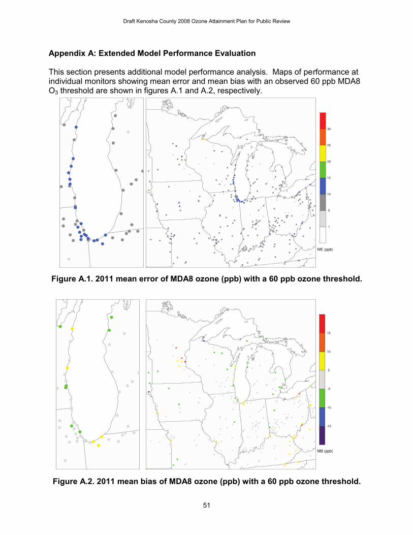
51
Appendix A: Extended Model Performance Evaluation This section presents additional model performance analysis. Maps of performance at individual monitors showing mean error and mean bias with an observed 60 ppb MDA8 O3 threshold are shown in figures A.1 and A.2, respectively.
Figure A.1. 2011 mean error of MDA8 ozone (ppb) with a 60 ppb ozone threshold.
Figure A.2. 2011 mean bias of MDA8 ozone (ppb) with a 60 ppb ozone threshold.
Draft Kenosha County 2008 Ozone Attainment Plan for Public Review
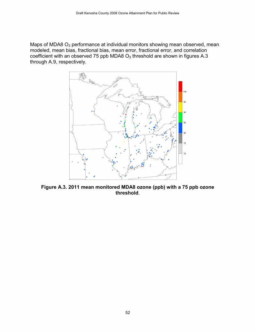
52
Maps of MDA8 O3 performance at individual monitors showing mean observed, mean modeled, mean bias, fractional bias, mean error, fractional error, and correlation coefficient with an observed 75 ppb MDA8 O3 threshold are shown in figures A.3 through A.9, respectively.
Figure A.3. 2011 mean monitored MDA8 ozone (ppb) with a 75 ppb ozone
threshold.
Draft Kenosha County 2008 Ozone Attainment Plan for Public Review
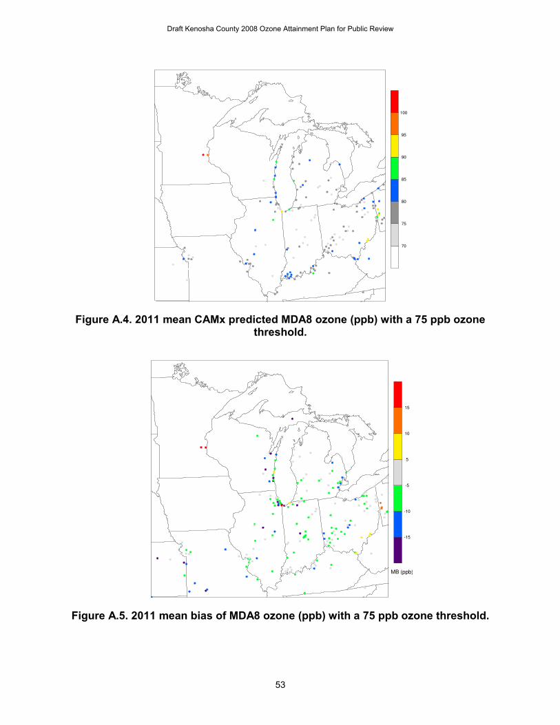
53
Figure A.4. 2011 mean CAMx predicted MDA8 ozone (ppb) with a 75 ppb ozone
threshold.
Figure A.5. 2011 mean bias of MDA8 ozone (ppb) with a 75 ppb ozone threshold.
Draft Kenosha County 2008 Ozone Attainment Plan for Public Review
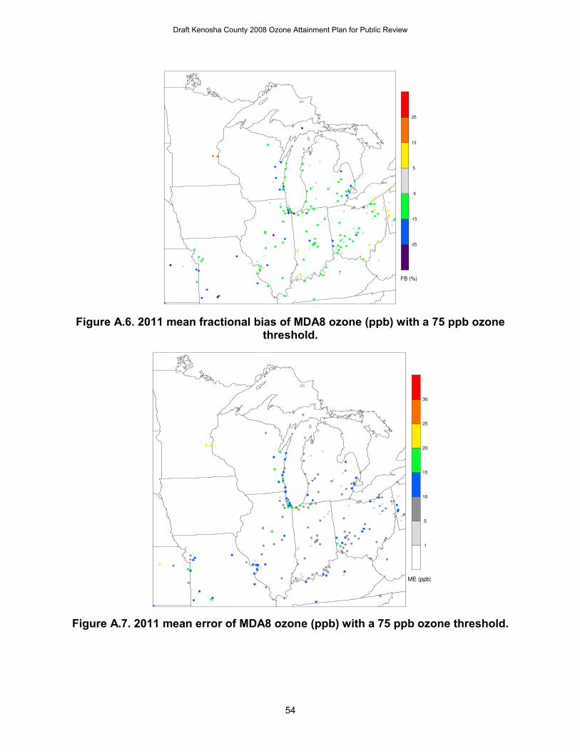
54
Figure A.6. 2011 mean fractional bias of MDA8 ozone (ppb) with a 75 ppb ozone
threshold.
Figure A.7. 2011 mean error of MDA8 ozone (ppb) with a 75 ppb ozone threshold.
Draft Kenosha County 2008 Ozone Attainment Plan for Public Review
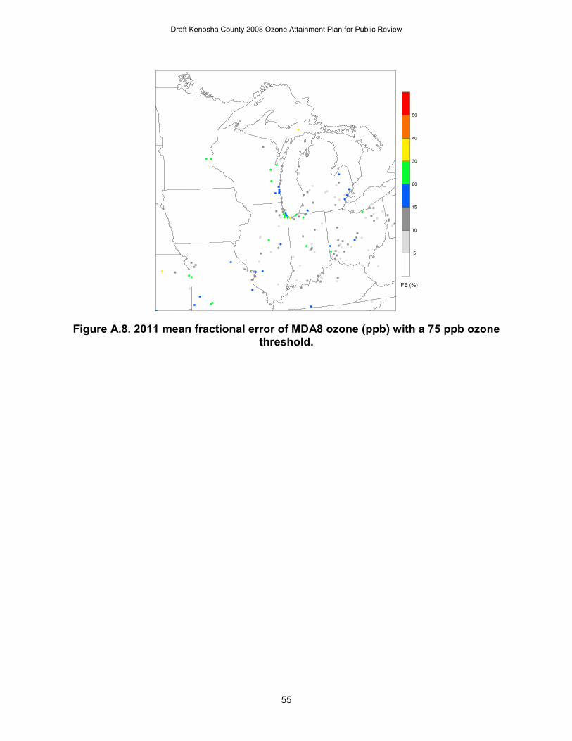
55
Figure A.8. 2011 mean fractional error of MDA8 ozone (ppb) with a 75 ppb ozone
threshold.
Draft Kenosha County 2008 Ozone Attainment Plan for Public Review
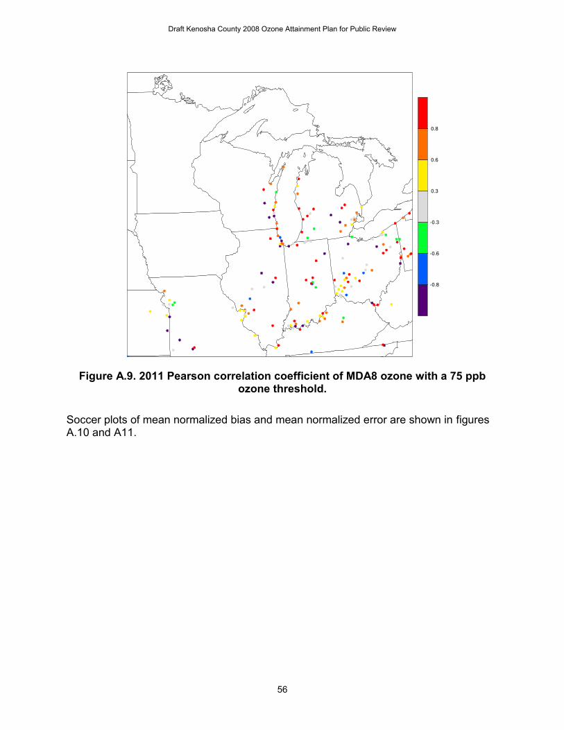
56
Figure A.9. 2011 Pearson correlation coefficient of MDA8 ozone with a 75 ppb
ozone threshold. Soccer plots of mean normalized bias and mean normalized error are shown in figures A.10 and A11.
Draft Kenosha County 2008 Ozone Attainment Plan for Public Review
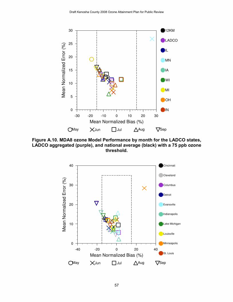
57
Figure A.10. MDA8 ozone Model Performance by month for the LADCO states, LADCO aggregated (purple), and national average (black) with a 75 ppb ozone
threshold.
Draft Kenosha County 2008 Ozone Attainment Plan for Public Review
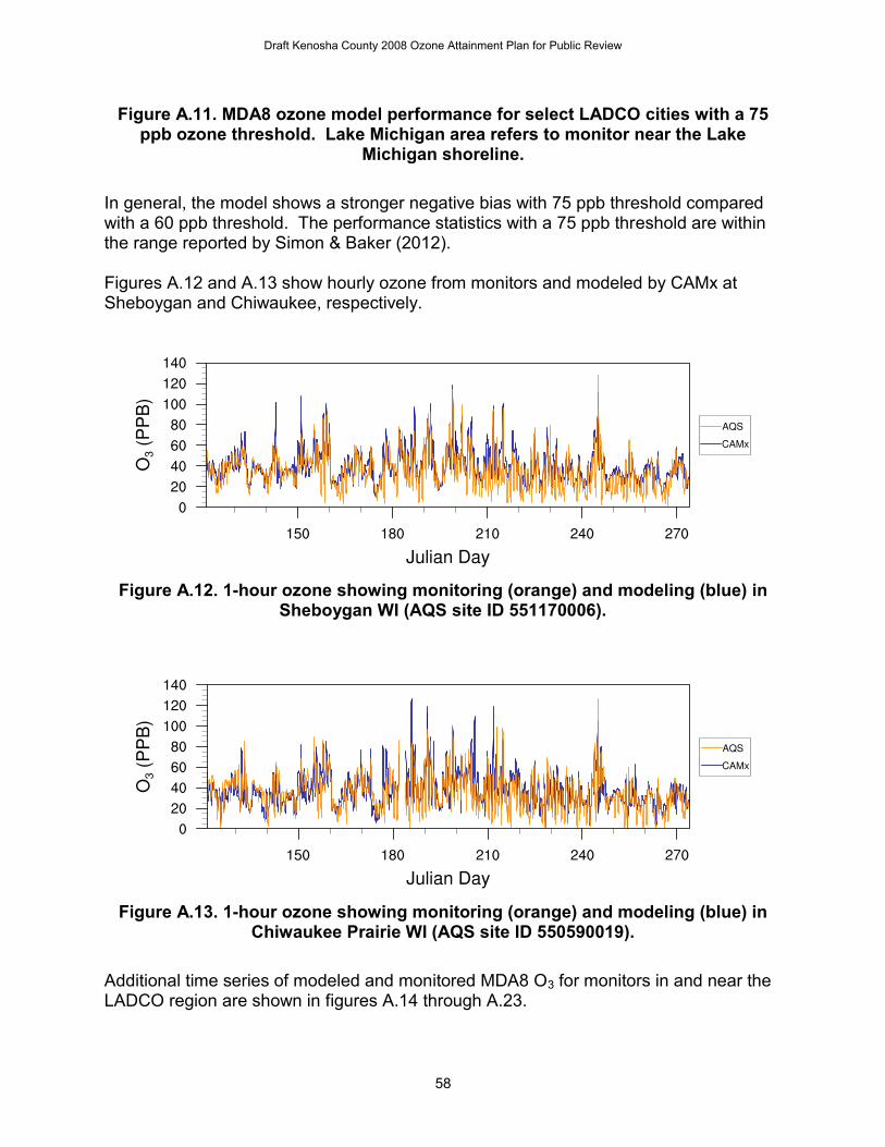
58
Figure A.11. MDA8 ozone model performance for select LADCO cities with a 75 ppb ozone threshold. Lake Michigan area refers to monitor near the Lake
Michigan shoreline. In general, the model shows a stronger negative bias with 75 ppb threshold compared with a 60 ppb threshold. The performance statistics with a 75 ppb threshold are within the range reported by Simon & Baker (2012). Figures A.12 and A.13 show hourly ozone from monitors and modeled by CAMx at Sheboygan and Chiwaukee, respectively.
Figure A.12. 1-hour ozone showing monitoring (orange) and modeling (blue) in
Sheboygan WI (AQS site ID 551170006).
Figure A.13. 1-hour ozone showing monitoring (orange) and modeling (blue) in
Chiwaukee Prairie WI (AQS site ID 550590019). Additional time series of modeled and monitored MDA8 O3 for monitors in and near the LADCO region are shown in figures A.14 through A.23.
Draft Kenosha County 2008 Ozone Attainment Plan for Public Review
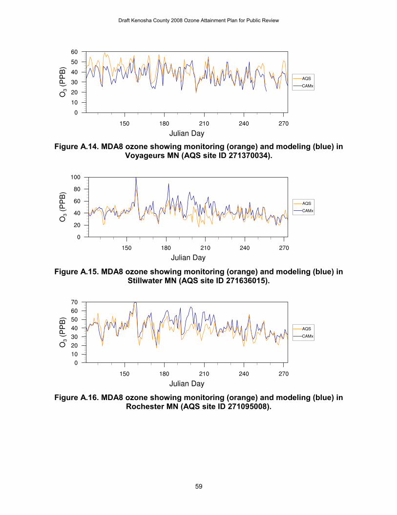
59
Figure A.14. MDA8 ozone showing monitoring (orange) and modeling (blue) in
Voyageurs MN (AQS site ID 271370034).
Figure A.15. MDA8 ozone showing monitoring (orange) and modeling (blue) in
Stillwater MN (AQS site ID 271636015).
Figure A.16. MDA8 ozone showing monitoring (orange) and modeling (blue) in
Rochester MN (AQS site ID 271095008).
Draft Kenosha County 2008 Ozone Attainment Plan for Public Review
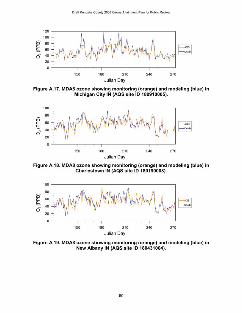
60
Figure A.17. MDA8 ozone showing monitoring (orange) and modeling (blue) in
Michigan City IN (AQS site ID 180910005).
Figure A.18. MDA8 ozone showing monitoring (orange) and modeling (blue) in
Charlestown IN (AQS site ID 180190008).
Figure A.19. MDA8 ozone showing monitoring (orange) and modeling (blue) in
New Albany IN (AQS site ID 180431004).
Draft Kenosha County 2008 Ozone Attainment Plan for Public Review
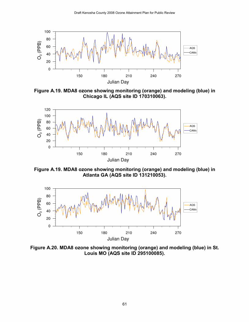
61
Figure A.19. MDA8 ozone showing monitoring (orange) and modeling (blue) in
Chicago IL (AQS site ID 170310063).
Figure A.19. MDA8 ozone showing monitoring (orange) and modeling (blue) in
Atlanta GA (AQS site ID 131210053).
Figure A.20. MDA8 ozone showing monitoring (orange) and modeling (blue) in St.
Louis MO (AQS site ID 295100085).
Draft Kenosha County 2008 Ozone Attainment Plan for Public Review
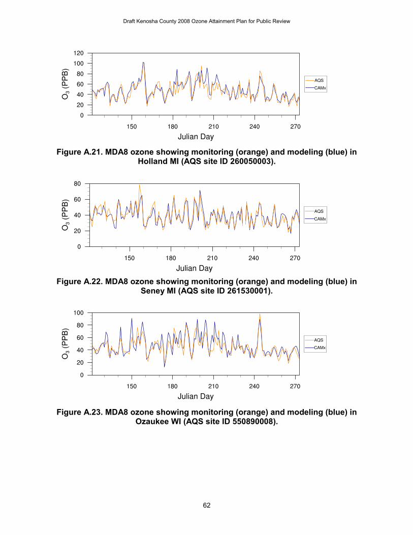
62
Figure A.21. MDA8 ozone showing monitoring (orange) and modeling (blue) in
Holland MI (AQS site ID 260050003).
Figure A.22. MDA8 ozone showing monitoring (orange) and modeling (blue) in
Seney MI (AQS site ID 261530001).
Figure A.23. MDA8 ozone showing monitoring (orange) and modeling (blue) in
Ozaukee WI (AQS site ID 550890008).
Draft Kenosha County 2008 Ozone Attainment Plan for Public Review
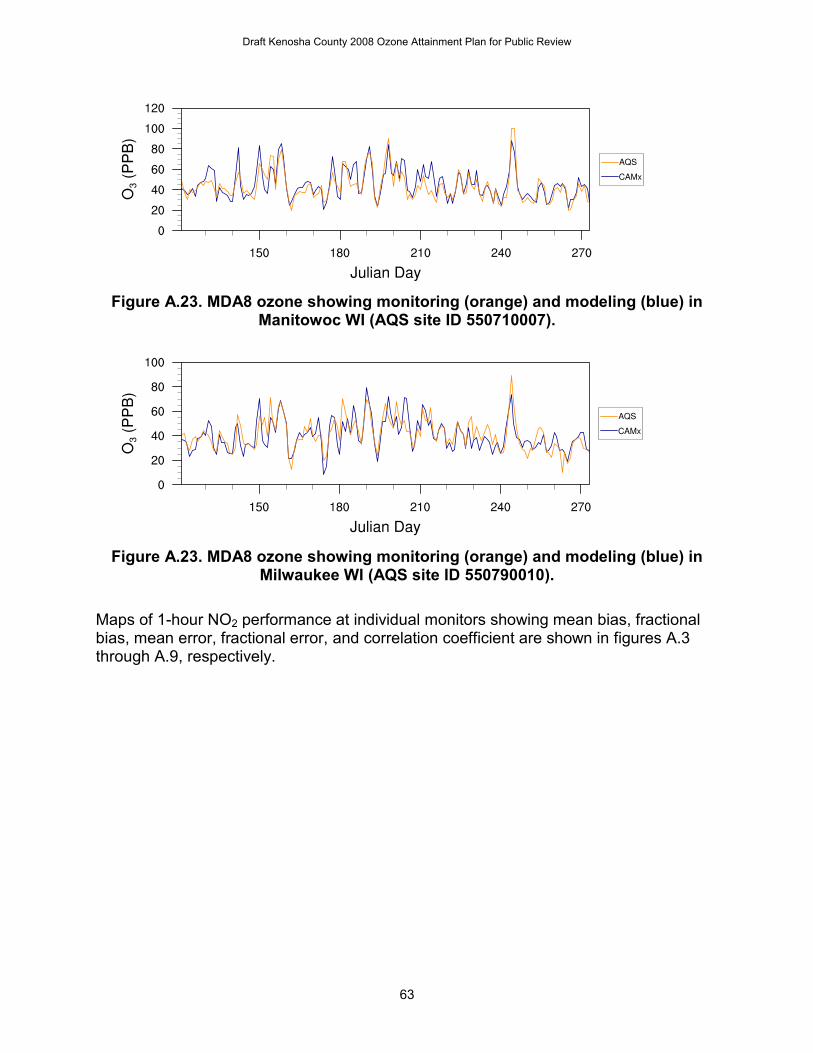
63
Figure A.23. MDA8 ozone showing monitoring (orange) and modeling (blue) in
Manitowoc WI (AQS site ID 550710007).
Figure A.23. MDA8 ozone showing monitoring (orange) and modeling (blue) in
Milwaukee WI (AQS site ID 550790010). Maps of 1-hour NO2 performance at individual monitors showing mean bias, fractional bias, mean error, fractional error, and correlation coefficient are shown in figures A.3 through A.9, respectively.
Draft Kenosha County 2008 Ozone Attainment Plan for Public Review

64
Figure A.24. 2011 mean bias of 1-hour NO2 (ppb).
Draft Kenosha County 2008 Ozone Attainment Plan for Public Review
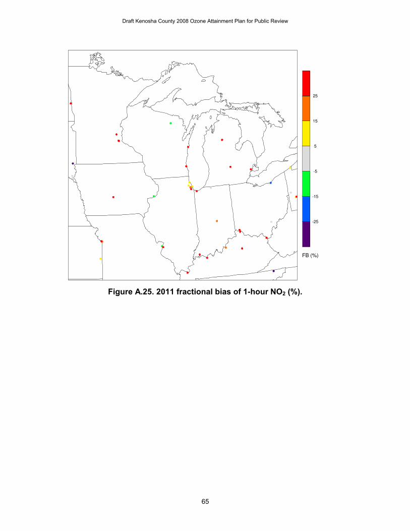
65
Figure A.25. 2011 fractional bias of 1-hour NO2 (%).
Draft Kenosha County 2008 Ozone Attainment Plan for Public Review
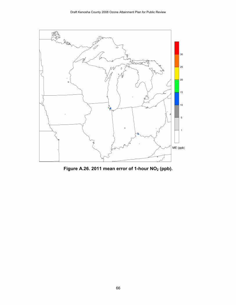
66
Figure A.26. 2011 mean error of 1-hour NO2 (ppb).
Draft Kenosha County 2008 Ozone Attainment Plan for Public Review
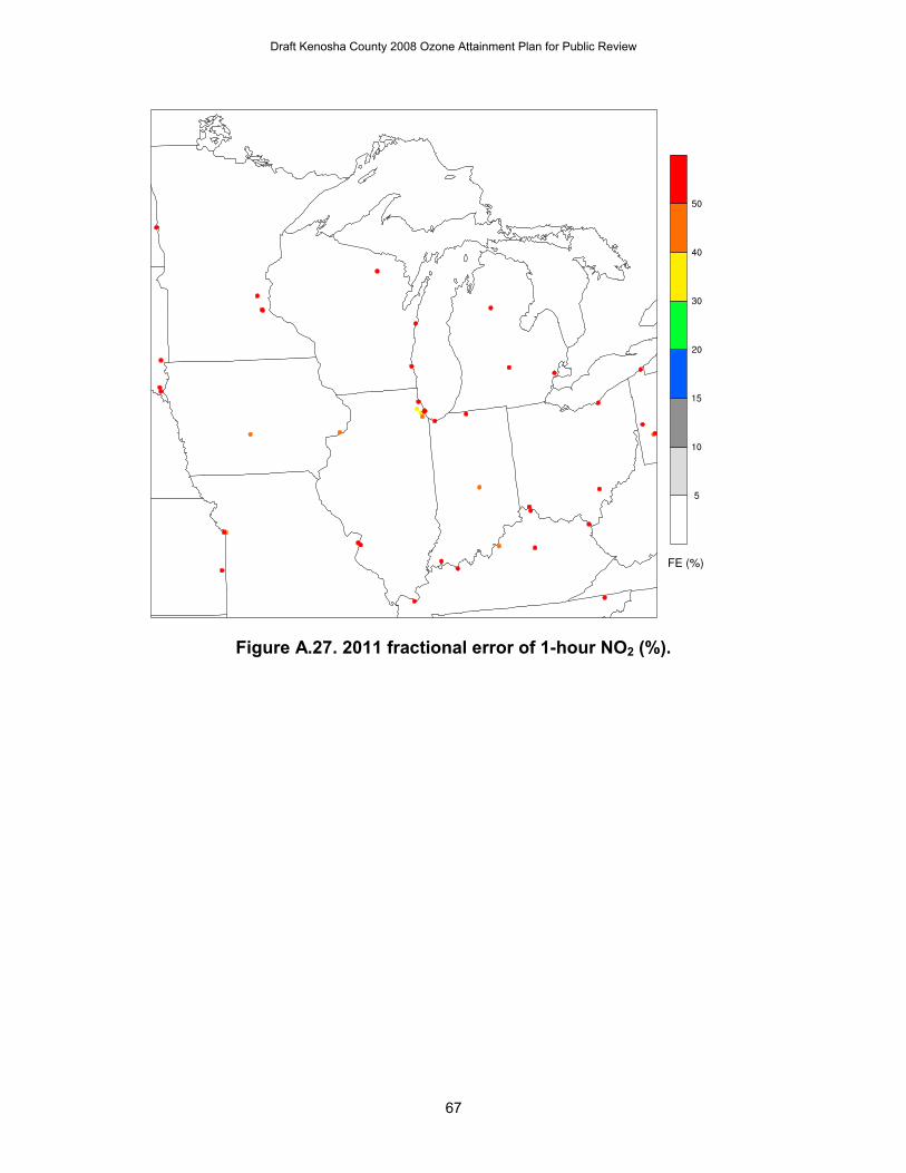
67
Figure A.27. 2011 fractional error of 1-hour NO2 (%).
Draft Kenosha County 2008 Ozone Attainment Plan for Public Review
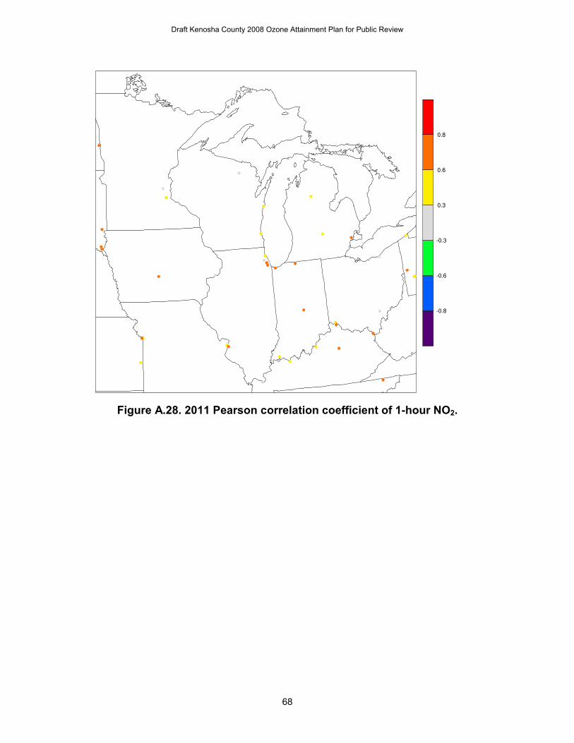
68
Figure A.28. 2011 Pearson correlation coefficient of 1-hour NO2.
Draft Kenosha County 2008 Ozone Attainment Plan for Public Review