Draft - tspace.library.utoronto.ca · Draft 2 20 Nonlinear Subgrade Reaction Solution for Circular Tunnel Lining Design Based 21 on Mobilized Strength of Undrained Clay 22 23 Abstract:

Draft

Nonlinear Subgrade Reaction Solution for Circular Tunnel

Lining Design Based on Mobilized Strength of Undrained Clay

Journal: Canadian Geotechnical Journal

Manuscript ID cgj-2017-0006.R1

Manuscript Type: Article

Date Submitted by the Author: 09-May-2017

Complete List of Authors: Zhang, Dongming; Tongji University, Dept. of Geotechnical Engineering

Phoon, Kok-Kwang; National University of Singapore, Department of Civil & Environmental Engineering Hu, Qunfang; Shanghai Institute of Disaster Prevention and Relief, Huang, Hongwei; Tongji University,

Keyword: subgrade reaction, tunnel, mobilized strength, undrained clay

https://mc06.manuscriptcentral.com/cgj-pubs

Canadian Geotechnical Journal

Draft

1

Nonlinear Subgrade Reaction Solution for Circular Tunnel Lining Design Based 1

on Mobilized Strength of Undrained Clay 2

3

Dong-ming Zhang 4

Assistant Professor, Key Laboratory of Geotechnical and Underground Engineering of 5

Minister of Education, and Department of Geotechnical Engineering, Tongji University, 6

Shanghai, China. Email: [email protected] 7

Kok-Kwang Phoon 8

Professor, Department of Civil and Environmental Engineering, National University of 9

Singapore, Blk E1A, # 07-03, 1 Engineering Drive 2, Singapore 117576. Email: 10

[email protected] 11

Qun-fang Hu 12

Associate Professor, Shanghai Institute of Disaster Prevention and Relief, Shanghai, China. 13

Email: [email protected] 14

Hong-wei Huang 15

Professor, Key Laboratory of Geotechnical and Underground Engineering of Minister of 16

Education, and Department of Geotechnical Engineering, Tongji University, Shanghai, China. 17

Email: [email protected] (Corresponding Author) 18

19

Page 1 of 57



Draft

2

Nonlinear Subgrade Reaction Solution for Circular Tunnel Lining Design Based 20

on Mobilized Strength of Undrained Clay 21

22

Abstract: 23

This paper presents a nonlinear solution of radial subgrade reaction–displacement (pk-ur) 24

curve for circular tunnel lining design in undrained clay. With the concept of soil shear 25

strength nonlinearly mobilized with shear strain, an analytical solution of pk is obtained using 26

the mobilized strength design (MSD) method. Two typical deformation modes are 27

considered, namely oval and uniform modes. A total of 197 orthogonally designed cases are 28

used to calibrate the proposed nonlinear solution of pk using the finite element method (FEM) 29

with the Hardening soil (HS) model. The calibration results are summarized using a 30

correction factor η, which is defined as the ratio of pk_FEM over pk_MSD. It is shown that η is 31

correlated to some input parameters. If this correlation is removed by a regression equation 32

f, the modified solution f×pk_MSD agrees very well with pk_FEM. Although the mobilized soil 33

strength varies with principal stress direction in reality, it is found that a simple average of 34

plane strain compression and extension results is sufficient to produce the above agreement. 35

The proposed nonlinear pk-ur curve is applied to an actual tunnel lining design example. 36

The predicted tunnel deformations agree very well with the measured data. In contrast, a 37

linear pk model would produce an underestimation of tunnel convergence and internal forces 38

by 2-4 times due to the overestimation of pk at large strain level. 39

40

Keywords: 41

Radial subgrade reaction, Tunnel, Mobilized strength design (MSD), Nonlinear, Undrained 42

clay. 43

44

Page 2 of 57



Draft

3

Introduction 45

The embedded beam spring model is the most frequently used design model among all the 46

models recommended by design codes for the structural design of tunnel linings (ITA 2004; 47

JSCE 2007; GB50157 2013). Some key aspects in lining design, e.g., soil load, lining 48

structure and soil-structural interactions, are considered explicitly in this model. 49

Specifically, the tunnel lining is represented by beams supported on soil springs around 50

tunnel perimeter to simulate the soil-structural interaction caused by initial earth pressure. 51

However, the soil spring constant, also named as the radial subgrade modulus kr, is difficult 52

to evaluate and it is often selected from empirical correlations with some engineering 53

judgment (Mair 2008). For example, the standard penetration test (SPT) blow count N has 54

been related to a range of kr in some local design regulations (JSCE 2007; DGJ08-10 2010). 55

It is a matter of judgment to pick a specific value of kr from this broad guideline, which 56

would translate to significant uncertainty in the calculated lining thrust and moment (Lee et al. 57

2001; Gong et al. 2015). Hence, some analytical solutions of kr have been proposed as a 58

more rational method to estimate the magnitude of this parameter for design (Arnau and 59

Molins 2011). 60

These analytical solutions of kr are usually derived with a basic assumption of elastic soil 61

in infinite or semi-infinite space. The value of kr is defined as the ratio of calculated 62

subgrade reaction pk over soil radial displacement ur around the tunnel perimeter given a 63

prescribed deformation mode of soil-lining interaction. Wood (1975) proposed a solution of 64

kr under the assumption of oval deformation mode shape in infinite space. Sagaseta (1987) 65

presented a solution of kr under a uniform deformation mode shape in semi-infinite space. 66

Later on, more general ground deformation modes are developed by combining these two 67

basic mode shapes (Verruijt and Booker 1996; Park 2005; Pinto and Whittle 2014). Based 68

on this observation, Zhang et al. (2014) proposed a general elastic solution of kr that can be 69

Page 3 of 57



Draft

4

decomposed into a series of basic kr, each produced by a simple soil deformation mode 70

shape. 71

However, it has been observed from centrifuge test results that tunneling may produce 72

non-linear soil behavior around the tunnel (Mair 1979; Taylor 1998). In addition, in-situ 73

measurements of tunnels in operation have shown that large deformations far beyond the 74

elastic range can happen (Shen et al. 2014). Huang and Zhang (2016) presented a detailed 75

field case where the tunnel deformation caused by extreme surface surcharge is almost seven 76

times larger than the design value. The large tunnel deformation inevitably will drive the 77

soil around the tunnel to an elasto-plastic state (Osman et al. 2006b; Klar et al. 2007). Thus, 78

the elastic solution of kr might not be sufficient to describe the full range of behavior of this 79

key input parameter in a tunnel lining design. Hence, there is a practical motivation to 80

develop an elasto-plastic solution of kr to model tunnel lining behavior in non-linear soils. 81

The task at hand is to obtain a non-linear solution of kr, which is a non-linear curve of 82

subgrade reaction pk versus the radial displacement ur. This is conceptually similar to the 83

well-known non-linear p-y curve for laterally loaded piles (Nogami et al. 1992; Bransby 1999; 84

McGann et al. 2011). However, unlike the p-y curve for laterally loaded pile design, limited 85

solutions have been proposed for the non-linear pk-ur curve for tunnel lining design. A 86

non-linear curve with the assumption of a hyperbolic function for subgrade reaction has been 87

proposed and utilized for the design of rock tunnel supports (Oreste 2007; Do et al. 2013; Do 88

et al. 2014). The rationality of using the hyperbolic shape function is not well described and 89

its relation to rock properties is unclear. 90

The mobilized strength design (MSD) method can provide a more rational method to 91

derive the non-linear pk-ur curve and can provide an explicit linkage to relevant soil 92

properties. The MSD method is built around an assumed plastic deformation mechanism of 93

the soil movements due to soil-lining interaction and the concept of “mobilized soil strength” 94

Page 4 of 57



Draft

5

that is founded on measured soil behavior (Bolton and Powrie 1988; Bolton et al. 1990). 95

For the problem with tunneling induced ground movement, Osman et al. (2006a) has 96

developed a non-linear curve of initial support pressure p varying with the ground surface 97

settlement sm by using the MSD method. The empirical Gaussian function (Peck 1969; 98

Osman et al. 2006b) is adopted to describe the ground movement in the model. However, 99

the soil-lining interactions that cause the common oval deformation mode (Klar et al. 2007; 100

Pinto et al. 2014) are ignored in their model. The MSD method is useful, because it 101

provides an analytical solution to a fairly complex soil-structure interaction problem. 102

Although the finite element method (FEM) can solve the same problem, it is arguably less 103

physically insightful than the MSD method and it may require a more detailed 104

characterization of soil behavior (in terms of parameters for constitutive model) beyond what 105

is produced by a routine site investigation. The cost of achieving analytical simplicity in the 106

MSD method is that it is potentially less accurate than the FEM (assuming all information 107

required in the FEM method is fully available). Nonetheless, Zhang et al. (2015) showed 108

that the MSD method and the FEM could produce comparable solutions if the former is 109

corrected by a simple factor. A key contribution of this paper is the characterization of this 110

correction factor for the tunnel lining problem. 111

The objective of this paper is to develop a non-linear curve of subgrade reaction pk varying 112

with radial displacement ur for a circular lined tunnel in elasto-plastic undrained soil using 113

the MSD method. The non-linear solution of radial subgrade modulus kr is derived as the 114

derivative of this pk-ur curve. The mobilized soil strain εmob is expressed as a function of 115

radial displacement ur using a typical uniform or oval deformation mode for soil-lining 116

interactions in semi-infinite space (Verruijt and Booker 1996). The subgrade reaction pk is 117

then calculated with the concept of mobilized soil strength su,mob under the minimum energy 118

principle. The finite element method (FEM) with a widely used nonlinear constitutive 119

Page 5 of 57



Draft

6

model for undrained soil, namely the Hardening Soil (HS) model, is adopted to validate the 120

applicability of the proposed nonlinear solution of pk. The MSD solution (pk_MSD) can be 121

corrected to agree with the FEM solution (pk_FEM) using a simple approach proposed in Zhang 122

et al. (2015). Finally, the performance of the corrected MSD method is demonstrated using 123

a tunnel lining design example based on a field case reported by Huang and Zhang (2016). 124

Deformation modes subjected to subgrade reaction 125

Mode shape for tunnel lining 126

A tunnel lining interacts with the surrounding ground after it is installed. It deforms 127

under the initial earth pressure coming from the ground. The ground responds to the lining 128

deformation by a subgrade reaction. The lining deformation would adjust to the subgrade 129

reaction and subsequently induce a new but small subgrade reaction. This iteration would 130

finally converge and the lining would form a specific distribution of deformation that is 131

consistent to the distribution of subgrade reaction. Although this distribution is complicated 132

and different from case to case, it could be reasonably characterized by basic mode shapes 133

such as uniform and oval shapes or more general shapes that can be viewed as combinations 134

of these basic mode shapes (Pinto and Whittle 2014; Pinto et al. 2014; Zhang et al. 2014). It 135

should be noted that all deformation mechanisms discussed in this paper take place under the 136

plane strain condition since a tunnel is a long linear structure. 137

In the case of a uniform mode shape (see in Fig. 1a), the lining deforms uniformly around 138

the tunnel perimeter at a constant value, saying ∆ (Sagaseta 1987): 139

1ru = ∆ (1a) 140

where ur1 means the uniform radial convergence at the perimeter of the tunnel lining. In the 141

case of an oval mode shape (see in Fig. 1b), the lining deforms following a cosine function of 142

the sectional angle θ with vertical axis, as shown below (Wood 1975): 143

2 cos 2ru δ θ= (1b) 144

Page 6 of 57



Draft

7

where ur2 means the oval radial convergence at tunnel perimeter. The parameter δ is the 145

value of deformation at the tunnel crown (i.e., θ = 0º). More general deformation shapes 146

can be formed by combining these two basic mode shapes. It is clear that the parameters ∆ 147

and δ are the maximum magnitude of the lining convergence around the tunnel perimeter. It 148

is more convenient to use these parameters as key performance indicators of the tunnel lining 149

under earth pressure including subgrade reaction, rather than to consider the entire shape. 150

It has been reported that these deformation indicators (i.e., ∆ and δ) are closely related to 151

the internal forces of lining and structural defects, e.g., crack, leakage, concrete spalling or 152

joint opening for segmental lining of shield tunnel (Yuan et al. 2012; Huang and Zhang 2016). 153

Large internal forces or severe structural defects could affect the serviceability and safety of 154

tunnels. Hence, it is not surprising these deformation indicators appear in the definition of 155

ultimate and serviceability limit states in tunneling codes and standards. For example, the 156

British Tunnel Standard (BTS 2004) has set an ultimate limit for the maximum convergence 157

normalized by tunnel radius (∆/R or δ/R, R is the tunnel radius) at 2%. As for serviceability, 158

the Chinese code (GB50157 2013) has set a serviceability limit of ∆/R (or δ/R) at 0.3%-0.4%, 159

while the Shanghai local regulation (DGJ08-10 2010) relaxes the serviceability limit to 0.5%. 160

Deformation modes for soils around the tunnel 161

Assuming that soil and tunnel lining deforms in a compatible way, one expects the soil 162

around the deformed tunnel to follow the two main deformation modes, namely uniform and 163

oval modes. Equations characterizing these two modes in infinite space and semi-infinite 164

space are available (Timoshenko and Goodier 1970; Wood 1975; Pinto and Whittle 2014). 165

Although these equations are derived analytically with a deformation field based on elasticity, 166

measured data reported in the literature have justified this assumption, namely the observed 167

deformation field for mobilized soils in a nonlinear state is proportional to those elastic 168

deformation fields (Mair 1979; Klar et al. 2007; Pinto et al. 2014). Since the mode in 169

Page 7 of 57



Draft

8

semi-infinite space is suitable for both the shallow and deep tunnels, it is applied to describe 170

the elasto-plastic deformation field of mobilized soils in this paper. Based on the solutions 171

proposed by Verruijt and Booker (1996), the uniform and oval deformation modes for 172

undrained soil with a Poisson’s ratio ν of 0.5 in semi-infinite space are briefly introduced 173

below. 174

a). Uniform mode 175

A typical uniform deformation field is plotted in Fig. 2a. The tunnel with a radius of R is 176

buried in a depth of h below the ground surface, as shown in Fig. 2a. The horizontal ground 177

movement ux could be represented by Eq. 2a, while the vertical ground movement uz could be 178

represented by Eq. 2b, as shown below: 179

22 2 2 2 2 2

4 ( )

( ) ( ) ( )x

x x xz z hu R

x z h x z h x z h

+ = −∆ ⋅ + −

+ − + + + + (2a) 180

2 2

22 2 2 2 2 2 2 2

2 ( )2( )

( ) ( ) ( ) ( )z

z x z hz h z h z hu R

x z h x z h x z h x z h

− +− + + = −∆ ⋅ + − + + − + + + + + +

(2b) 181

where x is the horizontal distance of calculated soil element from tunnel axis, and z is the 182

depth of the element. The parameter ∆ is the radial convergence of the deformed tunnel 183

lining in a uniform shape mentioned previously. Although the tunnel deforms uniformly, it 184

is clear from Fig. 2a that the surrounding soils do not deform uniformly due to the effect of 185

the image part of singularity solution in a semi-infinite space (Sagaseta 1987). 186

In a semi-infinite space, the boundary of the deformation field is located at the ground 187

surface above the tunnel. There is no boundary at the two sides of the tunnel and below the 188

tunnel. But it should be noted from Eq. 2 that, as the radial distance r between soil and the 189

center of tunnel increases, the soil displacement vanishes quickly following a decay function 190

of 1/r. That is to say, when the distance r is about 100 times of radius R, the corresponding 191

soil element would have a displacement less than 1% of ∆, which exert a negligible effect on 192

Page 8 of 57



Draft

9

the behaviors of soil around tunnel lining (Mair et al. 1993). 193

In this deformation mode, the calculation of soil strain by a first derivation of Eq. 2 have 194

revealed that the direction of principal strain is horizontal for soils locating above tunnel 195

crown and along its vertical axis, while the direction of principal strain is vertical for soils 196

locating at the two sides of the springline. It has been validated by ground movement in 1g 197

model test (Seneviratne 1979; Osman et al. 2006a). Hence, the soil behaviors along the 198

vertical axis are more likely to be modelled under the condition of plane strain extension 199

(PSE), while the soils at two sides of springline are to be modelled under the condition of 200

plane strain compression (PSC), as shown in Fig. 2b. 201

b). Oval mode 202

The typical oval deformation field is plotted in Fig. 3a. Similar to the uniform mode, the 203

tunnel has a radius of R and a cover depth of h. The horizontal ground movement ux is 204

expressed by Eq. 3a, and the vertical ground movement uz is represented by Eq. 3b, as shown 205

below: 206

( )( )

( )

( )

( )

( )

2 22 22 2

2 2 32 22 2 2 2

2 ( ) 3 24

2 2x

x x h z h z x h zx x zu R xh

x z x h z x h z

δ − − − − −− = − ⋅ + −

+ + − + −

(3a) 207

( )( )

( )

( )

( )

( )

( )

( )

2 22 22 2

2 2 22 22 2 2 2

22

322

(2 ) 2 22

2 2

( )(2 ) 3 24

2

z

h z x h z x h zz x zh

x z x h z x h zu R

h z h z x h zh

x h z

δ

− − − − −− − + − + + − + −

= ⋅ − − − − −

+ −

(3b) 208

where x is the horizontal distance between the calculated soil element and the tunnel axis, and 209

z is the depth of the element. The parameter δ is the magnitude of lining displacement at 210

crown as the tunnel deforms into an oval shape mentioned previously. Similar to the case of 211

uniform mode, the boundary of the oval mode is located at the ground surface above tunnel, 212

and the soil displacement will decrease with the increase of radial distance r following a 213

Page 9 of 57



Draft

10

decay function of 1/r. 214

In the oval deformation mode, similar to the case of uniform mode, the calculated 215

principal strain of soil along the vertical axis from Eq. 3 is in the horizontal direction. The 216

soil at both sides of the springline experiences principal strains in the horizontal direction due 217

to the extension of soil at the springline location as part of an oval shape. This extension 218

ground movement mode at the springline location can be seen from measured data in field 219

cases (Hashimoto et al. 1996; Standing and Selemetas 2013). Hence, the plane strain 220

extension (PSE) condition is more suitable for modeling mobilized soil behavior in an oval 221

mode, as shown in Fig. 3b. 222

Energy Conservation in Mobilized Soils 223

Following the MSD concept that the soil is in continuous yielding corresponding to a 224

mobilized strength, the potential energy loss caused by deformed soil induced by soil-lining 225

interaction is equal to the work done by corresponding subgrade reaction load pk around the 226

tunnel perimeter. This energy conservation formulation is the same as those general 227

formulation used for elastic solutions of subgrade reaction (Verruijt and Booker 1996; Zhang 228

et al. 2014). It should be emphasized that this energy conservation formulation only 229

accounts for soil-lining interaction at a distance behind the tunnel face. It does not include 230

the work done by the face support pressure during tunnel excavation. The MSD framework 231

for this tunneling procedure has been presented elsewhere by Osman et al. (2006a) and Klar 232

and Klein (2014). With the above consideration in mind, the formulation of energy 233

conservation for subgrade reaction can be expressed as below: 234

,k r u mob sD Area

p u ds s dAπ

ε=∫ ∫ (4) 235

where the ur is soil radial displacement around the tunnel perimeter calculated by using the ux 236

and uz mentioned previously (ur=uzcosθ-uxsinθ). The one-dimensional integral length for 237

left side of Eq. 4 is essentially along the tunnel perimeter i.e., πD in Eq. 4, while the 238

Page 10 of 57



Draft

11

two-dimensional integral area for the right side, i.e., Area in Eq. 4, is the semi-infinite space 239

described in previous section (see Fig. 1). The parameters su,mob and εs are the mobilized 240

soil undrained shear strength and the corresponding mobilized engineering shear strain, 241

respectively. Adopting the rule-of-thumb that the engineering shear strain εs is 1.5 times of 242

the deviatoric strain εq leads to: 243

31.5 , ( , principal directions)

2s q ij ij i jε ε ε ε= = (5) 244

where εij are the shear strain in the principal directions. All these strains could be calculated 245

by Eqs. 2 and 3 in closed form. The mobilized undrained shear strength su,mob is obtained by 246

a suitable nonlinear interpolation of the stress-strain curve given a calculated mobilized 247

engineering shear strain εs for each soil element within the semi-infinite integral area. The 248

soil elements around tunnel are in a PSC, PSE, or an intermediate state, depending on the 249

rotation of the principal strain. Hence, soils within the integral area in the right side of Eq. 4 250

theoretically should be discretized into separate soil element that follows a stress-strain curve 251

compatible to the rotation of the principal strain calculated by Eqs. 2 and 3. In other words, 252

for this tunnel problem, the stress-strain curve varies with spatial location, because the 253

rotation of the principle strain varies with spatial location. 254

Practical Approximation of Energy Conservation 255

It is evident that the exact solution of Eq. 4 can be tedious if each soil element is assigned 256

a stress strain curve as a function of the principal strain rotation at each location. A practical 257

solution to Eq. 4 is to examine the possibility of replacing su,mob which varies according to 258

principal strain rotation by an equivalent s*u,mob that does not depend on principal strain 259

rotation. Since both PSC and PSE states are present in the soil elements around the 260

deformed tunnel (as see in Fig. 2b), a simple way to approximate the exact mobilized shear 261

strength su,mob is to average the results of su,mob from plane strain compression tests and the 262

results of su,mob from plane strain extension tests, as recommended by Koutsoftas and Ladd 263

Page 11 of 57



Draft

12

(1985): 264

*

, , ,0.5( )

PSE PSCu mob u mob u mob

s s s= + (6) 265

Note that both the su,mob׀PSE from plane strain extension test and su,mob׀PSC from plane strain 266

compression tests are evaluated at the depth of the tunnel axis following the assumption 267

adopted by Osman and Bolton (2006a) for a tunneling-induced ground settlement problem. 268

The mobilized shear strength su,mob in Eq. 4 could be replaced by the above approximate 269

s*

u,mob in Eq. 6. It is worth pointing out here that the fundamental value of MSD is related to 270

its ability to produce an answer sufficiently accurate for design at a significantly lower cost 271

than FEM. If MSD is only marginally less costly than FEM, there is no reason to adopt MSD. 272

Eq. 6 is adopted with this pragmatic consideration in mind. The focus of this study is to 273

clarify if the error associated with this approximation as benchmarked against the finite 274

element solution is acceptable for design purposes. 275

In addition, when Eq. 4 is integrated numerically, the semi-infinite space is approximated 276

by a large circular domain with a radius about 100 times the tunnel radius R, which is 277

reasonably large enough to minimize the effect of ignoring soil displacements outside this 278

domain on the integral results (Klar et al. 2007). Hence, equation 4 is re-written based on 279

the above simplification as follows: 280

{ }*

, ( 0, 100 )k r u mob sD Area

p u ds s dA Area z r Rπ

ε= ∈ ≥ ≤∫ ∫ (7) 281

As the tunnel lining deforms into a prescribed mode shape (uniform or oval), the 282

distribution of subgrade reaction would match a similar shape to the deformation shape 283

following the basic Winkler assumption. Hence, two distribution shapes for subgrade 284

reaction pk is assumed based on the previously assumed deformation shapes, namely the 285

uniform and oval shapes. Equation 7 is further developed based on each specific 286

deformation mode below. 287

In the case of the uniform mode, subgrade reaction pk is distributed with a constant value 288

Page 12 of 57



Draft

13

pk0 at any position along lining as below: 289

0k kp p= (8) 290

By substituting Eq. 8 and Eq. 1a into Eq. 7, the pk0 can be derived as following equation: 291

( )*

,

0

u mob sArea

k

D

s dAp

dsπ

ε× ∆=

∆∫

∫ (9) 292

where ∆ is the radial displacement of lining under uniform shape (see in Eq. 1a). When 293

given a specific value of ∆, the engineering shear strain εs could be derived by Eq. 5. The 294

approximate mobilized shear strength s*u,mob can then be read off a representative shear 295

stress-strain curve from Eq. 6 corresponding to the calculated εs. It is worth pointing out 296

that the stress-strain curve is an input obtained from an actual laboratory test. Subsequently, 297

subgrade reaction is derived by using Eq. 9. Hence, subgrade reaction pk is a nonlinear 298

function of the parameter ∆ given a specific soil stress-strain curve from the average of the 299

PSC test and PSE test. The subgrade modulus kr is just the first-order derivative of Eq. 9 300

with parameter ∆. 301

In the case of oval shape, subgrade reaction pk is distributed in an oval shape represented 302

by following equation: 303

0 cos 2k kp p θ= (10) 304

where pk0 is the subgrade reaction at tunnel crown and the angle θ is equal to zero. By 305

substituting Eq. 1b and Eq. 10 into Eq. 7, the pk0 is further derived as below: 306

( )*

,

0 2cos 2

u mob sArea

k

D

s dAp

dsπ

ε δ

δ θ

⋅= ∫

∫ (11) 307

where δ is the tunnel radial displacement at tunnel crown (see in Eq. 1b). Similar to the 308

uniform case, when the parameter δ is obtained, the subgrade reaction pk0 is derived as a 309

function of radial displacement δ given a specific soil stress-strain curve from the average of 310

the PSE and PSC tests. Subgrade modulus kr under oval mode is also obtained from the 311

Page 13 of 57



Draft

14

first-order derivative of Eq. 11. 312

Validation of Proposed Nonlinear Solution of pk 313

The proposed nonlinear subgrade reaction pk is derived analytically using the mobilized 314

strength concept and an approximate mobilized shear strength s*

u,mob that is independent of 315

principal strain rotation. In this section, this nonlinear subgrade reaction pk is validated by 316

comparing with the numerical result of pk from a two-dimensional finite element method 317

(FEM) analysis. A homogeneous soil condition is assumed in FEM and MSD to simplify 318

the validation. The FEM analysis requires a soil constitutive model, such as the Hardening 319

soil (HS) model. The MSD does not require a soil constitutive model. In practice, it uses 320

the measured laboratory test data from the average of PSE and PSC test results. In this 321

section, the PSE and PSC stress-strain curves are calculated numerically using a commercial 322

FEM code PLAXIS2D (Brinkgreve et al. 2006) on an element extracted at the depth of tunnel 323

axis with an element length, width and height equal to 1m×1m×1m. The same Hardening 324

soil (HS) model is used in this numerical element soil test. Hence, given a prescribed 325

displacement ur, the analytical pk0 is calculated by using Eqs. 9 and 11 with a calculated 326

stress-strain curve from the average of numerical PSC and PSE test results. 327

The PLAXIS2D code is also used for FEM analysis. Figure 4 is a representative finite 328

element mesh used in this paper. A tunnel with radius R of 3m is buried 22m below the 329

ground surface. The cover depth h is thus equal to 25m. Due to the symmetrical feature of 330

this problem, only half of the model is established as shown in Fig. 4a. The half-width and 331

depth of the mesh is equal to 200m and 120m, respectively, which are sufficiently large to 332

minimize boundary effects. The horizontal displacement along the vertical boundaries at 333

two sides of the mesh are constrained, while the vertical displacement along the horizontal 334

boundary at the bottom of mesh is constrained. An example of stress boundary conditions 335

following Eqs. 8 and 10 is shown in Fig. 4b and 4c. 336

Page 14 of 57



Draft

15

The input stress boundary around the tunnel perimeter is the subgrade reaction pk. The 337

response obtained from PLAXIS2D with a specific constitutive soil model (Hardening soil 338

model) is the soil radial displacement ur at the tunnel crown. Note that the radial subgrade 339

modulus kr varies around the tunnel perimeter – it is smaller at the tunnel crown than at the 340

invert (Verruijt 1997). In other words, a uniform subgrade reaction around the tunnel 341

perimeter produces a larger soil radial displacement ur and consequently a smaller subgrade 342

modulus kr (i.e., kr = pk / ur) at the tunnel crown compared to the results at other positions 343

around the tunnel perimeter. Hence, a design based on the smallest subgrade modulus kr at 344

the tunnel crown would be most conservative, i.e. the calculated internal lining forces are the 345

highest. This study focuses on the nonlinear pk versus ur curve at the tunnel crown for this 346

reason. 347

The Hardening soil (HS) model that is widely used in tunnel designs is selected for this 348

validation study. The HS model is essentially a hyperbolic nonlinear model that considers 349

both shear hardening and compression hardening. Details of this soil model are given 350

elsewhere (Möller and Vermeer 2008). Typical stress strain curves for HS model are 351

illustrated in Fig. 5, i.e., solid line for the plane strain compression condition and dash line for 352

the plane strain extension condition. The average mobilized strength obtained by averaging 353

the results from both PSC and PSE tests is also plotted against shear strain in Fig. 5 as the 354

dot-dash line. A set of input soil parameters required for HS model are provided in Table 1 355

for typical undrained Shanghai soft clay following the suggestion by Zhang et al. (2015). 356

Note that the soil unit weight input for FEM analysis is set to zero because the work done by 357

soil weight is not included in the energy conservation equation (see in Eq. 4). Undrained 358

analysis with undrained strength parameter (su) (method B in Plaxis) is carried out in this 359

validation study. For method B in PLAXIS, note that the stiffness modulus is no longer 360

stress level dependent, because the effective friction angle is equal to zero. Hence, the HS 361

Page 15 of 57



Draft

16

model adopted in this paper exhibits no compression hardening. As a result, the soil used in 362

FEM model exhibits homogeneous soil stiffness. But the model retains its 363

unloading-reloading modulus and shear hardening characteristics. The nonlinear shear 364

hardening in the HS model contributes to the nonlinear mobilization of the soil undrained 365

shear strength. 366

Comparison with FEM Analysis 367

Figure 6 compares the calculated nonlinear curve of pk0-ur between MSD and FEM under 368

the uniform deformed shape condition. The horizontal axis refers to the ratio of the tunnel 369

convergence ∆ over the tunnel radius R, and the vertical axis refers to the representative 370

subgrade reaction pk0 at tunnel crown. The solid square dots in Fig. 6 are the FEM results 371

pk0_FEM from PLAXIS, and the solid line denotes the MSD results pk0_MSD with s*u,mob 372

determined from the average of su,mob from PSC and PSE test condition. It is clear from Fig. 373

6 that the MSD results pk0_MSD using an average stress strain curve is almost equal to the 374

numerical results of pk0_FEM. Thus, the approximation s*u,mob composed by the average of 375

PSC and PSE test results (Eq. 6) appears to be reasonable for this example. Similar findings 376

have also be presented for the tunneling-induced ground movement calculation where the 377

same approximation of mobilized strength is adopted (Osman et al. 2006a). 378

In addition, the linear elastic solution pk0_linear presented by Verruijt and Booker (1996) and 379

Zhang et al. (2013) is also plotted against the convergence ratio (∆/R) in Fig. 6 (denoted by 380

dotted lines). When the ∆/R is relatively small, say within a value of 0.1-0.2%, the 381

nonlinear pk0_MSD is almost equal to the linear solution, which shows that the nonlinear 382

solution reduces correctly to the linear solution at small strain level. However, the 383

nonlinearity of pk0_MSD could become significant as the tunnel convergence increases. The 384

shape of nonlinear variation of pk with ∆ is similar to the nonlinear shape of stress strain 385

curve. Hence, these figures indicate that linear pk0_linear is only appropriate for the design of 386

Page 16 of 57



Draft

17

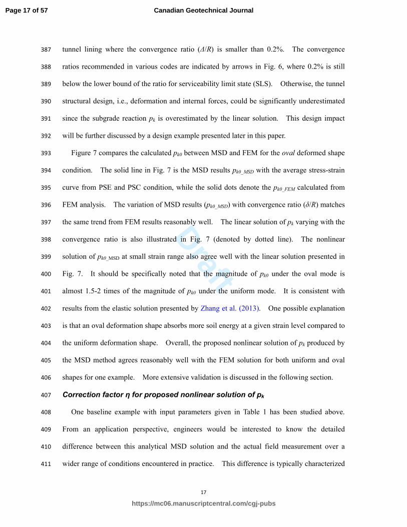
tunnel lining where the convergence ratio (∆/R) is smaller than 0.2%. The convergence 387

ratios recommended in various codes are indicated by arrows in Fig. 6, where 0.2% is still 388

below the lower bound of the ratio for serviceability limit state (SLS). Otherwise, the tunnel 389

structural design, i.e., deformation and internal forces, could be significantly underestimated 390

since the subgrade reaction pk is overestimated by the linear solution. This design impact 391

will be further discussed by a design example presented later in this paper. 392

Figure 7 compares the calculated pk0 between MSD and FEM for the oval deformed shape 393

condition. The solid line in Fig. 7 is the MSD results pk0_MSD with the average stress-strain 394

curve from PSE and PSC condition, while the solid dots denote the pk0_FEM calculated from 395

FEM analysis. The variation of MSD results (pk0_MSD) with convergence ratio (δ/R) matches 396

the same trend from FEM results reasonably well. The linear solution of pk varying with the 397

convergence ratio is also illustrated in Fig. 7 (denoted by dotted line). The nonlinear 398

solution of pk0_MSD at small strain range also agree well with the linear solution presented in 399

Fig. 7. It should be specifically noted that the magnitude of pk0 under the oval mode is 400

almost 1.5-2 times of the magnitude of pk0 under the uniform mode. It is consistent with 401

results from the elastic solution presented by Zhang et al. (2013). One possible explanation 402

is that an oval deformation shape absorbs more soil energy at a given strain level compared to 403

the uniform deformation shape. Overall, the proposed nonlinear solution of pk produced by 404

the MSD method agrees reasonably well with the FEM solution for both uniform and oval 405

shapes for one example. More extensive validation is discussed in the following section. 406

Correction factor η for proposed nonlinear solution of pk 407

One baseline example with input parameters given in Table 1 has been studied above. 408

From an application perspective, engineers would be interested to know the detailed 409

difference between this analytical MSD solution and the actual field measurement over a 410

wider range of conditions encountered in practice. This difference is typically characterized 411

Page 17 of 57



Draft

18

by a model factor (ratio of measured pk over the calculated value) in geotechnical reliability 412

based design (Phoon and Kulhawy 2005). Strictly speaking, the numerical subgrade 413

reaction pk from FEM analysis is not equal to the measured pk, but comparisons between 414

FEM solutions and field data for a number of geotechnical structures indicate that this 415

difference (i.e., model factor εFEM) is small. Several calibrations of finite element analysis 416

including finite element limit analysis (FELA) with field cases or physical model tests show 417

that mean of εFEM is between 0.95 and 1.01 and COV is between 0.06 and 0.18, as shown in 418

Table 2 (Phoon and Tang 2015a, 2015b; Tang and Phoon 2016a, 2016b, 2017). It is 419

reasonable to say that mean and COV of εFEM should be around 1 and around 0.1, respectively. 420

Nonetheless, to maintain a strict distinction between FEM solutions and field measurements, 421

Zhang et al. (2015) defined a ratio of FEM solution over calculated MSD value as a 422

correction factor. The model factor can be constituted as the product of the correction factor 423

and the model factor for FEM (typically unbiased, i.e. mean close to 1 and precise, i.e. 424

coefficient of variation around 10%). The purpose of this section is to characterize the 425

correction factor for the nonlinear analytical solution of pk using the method proposed in 426

Zhang et al. (2015). The characterization of the correction factor for the oval mode shape is 427

presented in detail below. 428

It is clear from Eqs. 2, 3, 9 and 11 that the calculated nonlinear solution pk depends on the 429

input parameters such as cover depth h, tunnel diameter D (or radius R), soil undrained shear 430

strength su and convergence deformation δ. Besides, the mobilized stress-strain curve could 431

also contribute to the evaluation of pk in the calculation. Because the Hardening Soil model 432

is applied, the soil unload-reloading modulus Eur is also included as an input parameter. In 433

summary, a total of four dimensionless parameters from the above five parameters are 434

considered in the orthogonal design of numerical cases required for characterization of the 435

correction factor, i.e., cover depth ratio h/D, undrained strength ratio su/σv’, soil 436

Page 18 of 57



Draft

19

unload-reloading modulus ratio Eur/su, and the tunnel convergence ratio δ/R. 437

Table 3 shows the typical ranges of these four parameters for tunnels in soft undrained 438

clay condition. The 197 numerical cases are designed in two stages. In the first stage, only 439

the parameters h/D, su/σv’, Eur/su are included to generate 25 orthogonal FEM models. Each 440

parameter has five different levels. In the second stage, for each one of the generated 25 441

models, different levels of convergence ratio (δ/D) are generated within the range of 0.001% 442

– 3%, i.e., typical range of tunnel deformation on site (Huang et al. 2016). Similar to the 443

procedure carried out for the baseline example, the pk is prescribed as the stress boundary 444

condition for FEM model in PLAXIS2D, while the calculated displacement δ from 445

PLAXIS2D is applied as an input parameter for MSD calculation to obtain an analytical 446

solution of pk. In total, there are 197 cases generated using these two-stage orthogonal 447

design principle. 448

Figure 8 plots the calculated pk from MSD (denoted as pk_MSD hereon) against the 449

prescribed pk in FEM model (denoted as pk_FEM hereon) for the 197 cases in a logarithm form 450

of the axes, denoted by grey square dots. It is observed from Fig. 8 that the pk_MSD 451

distributed relatively closely around the 45 degree line (i.e., the equality line pk_MSD = pk_FEM). 452

However, it is evident from Fig. 8 that the discrepancy between grey dots and 45 degree line 453

becomes larger as the absolute value of pk increases. To characterize this discrepancy 454

statistically, the correction factor η is defined as the ratio of the magnitude of pk_FEM over the 455

magnitude of pk_MSD. 456

_

_

k FEM

k MSD

p

pη = (12) 457

The model factor for pk_MSD is related the correction factor η as follows: 458

_ _ _

_ _ _

k m k FEM k m

MSD FEM

k MSD k MSD k FEM

p p p

p p pε η ε= = × = × (13) 459

where pk_m is the measured subgrade reaction. Table 2 shows that the mean and coefficient 460

Page 19 of 57



Draft

20

of variation (COV) of εFEM is close to 1 (unbiased) and relatively small (less than 20%) for a 461

number of different geotechnical systems studied thus far. The mean of η for the 197 cases 462

is equal to 1.02, which means the calculated pk_MSD is almost equal to the pk_FEM on the 463

average. The minimum and maximum value of η are 0.66 and 1.28, respectively, as shown 464

by the grey dashed lines in Fig. 8. The COV of the correction factor η is 0.15, which is 465

quite small compared to the MSD for other geotechnical structures, e.g., 0.47 for cantilever 466

deflection as shown in Table 2 (Zhang et al. 2015). The mean and COV of the correction 467

factor η for a variety of geotechnical problems such as foundation systems in different type of 468

soils (Table 2) appear to be around 1 and 0.10, respectively. 469

It is worthwhile to examine if the correction factor η is dependent on input parameters, 470

because it is clearly dependent on the magnitude of pk as shown in Fig. 8. The customary 471

practice for engineers to correct for model bias using the average model factor (deterministic 472

method) or as a random variable (reliability method) is only correct when the model factor is 473

random. To clarify this critical dependency issue, the calculated correction factor η is 474

plotted against the four input parameters h/D, su/σv’, Eur/su and δ/R as shown in Fig. 9a, 9b, 9c 475

and 9d, respectively. Note that the vertical axis in Fig. 9a – 9c is represented by averaged 476

correction factor ηave,i for 25 orthogonally designed FEM models in the first stage, which is 477

calculated as below: 478

,

,

m

i j

j

ave im

ηη =

∑ (14) 479

where ηi,j is the calculated correction factor for the total of 197 designed FEM cases, i is 480

equal to 1, 2, …, 25 which stands for the number of 25 orthogonal designed case in the first 481

stage, and j is equal to 1, 2, …, m which stands for the number of m cases in the second stage 482

given the parameter set of h/D, su/σv’, Eur/su have been selected in the first stage. For 483

example, the averaged ηave,1 is obtained by taking the arithmetic average of η1,j values from 6 484

Page 20 of 57



Draft

21

simulations (i.e., m = 6) with the following input parameters: 485

1. h/D = 2, su/σv’ = 0.5, Eur/su = 200, δ/R = 0.025%, η1,1 = 0.91; 486

2. h/D = 2, su/σv’ = 0.5, Eur/su = 200, δ/R = 0.061%, η1,2 = 0.94; 487

3. h/D = 2, su/σv’ = 0.5, Eur/su = 200, δ/R = 0.122%, η1,3 = 0.97; 488

4. h/D = 2, su/σv’ = 0.5, Eur/su = 200, δ/R = 0.242%, η1,4 = 1.02; 489

5. h/D = 2, su/σv’ = 0.5, Eur/su = 200, δ/R = 0.605%, η1,5 = 1.15; 490

6. h/D = 2, su/σv’ = 0.5, Eur/su = 200, δ/R = 1.419%, η1,6 = 1.19; 491

Thus, the calculated averaged ηave,1 is equal to 1.04, i.e., (0.91+0.94+0.97+1.02+1.15+1.19)/6. 492

By doing so, the averaged correction factor ηave is plotted against the input parameters in Fig. 493

9a to 9c. It is clear that ηave is strongly dependent on the cover depth ratio h/D, but is 494

relatively independent of strength ratio su/σv’ and modulus ratio Eur/su. The dependency of 495

ηave on the parameter h/D seems to follow a sigmoid function. In Fig. 9d, the calculated 496

correction factor η for all the 197 cases is plotted directly against δ/D on a logarithm scale. 497

A linear correlation between η and ln(δ/R) is obtained as shown in Fig. 9d. By conducting 498

Spearman correlation tests for all these four parameters, the p-value associated with a null 499

hypothesis of zero-rank (Spearman) correlation is much less than the strict 1% level of 500

significance for parameter h/D and δ/R. Hence, the null hypothesis that the correction factor 501

η is independent of the input parameter h/D and δ/R can be rejected at a level of significance 502

of 1%. 503

Because the correction factor is correlated to two input parameters, it cannot be modeled 504

as a random variable (Phoon and Kulhawy 2005). Figure 9 indicates that the correction 505

factor η varies with the input parameter h/D as a sigmoid function and varies with the input 506

parameter ln(δ/R) as a linear function. This systematic variation should be removed by 507

regression. Based on the above observed trends, the proposed regression equation is: 508

Page 21 of 57



Draft

22

1

0 1 2 3exp ( ln )h

f a a a aD R

δ− = + × +

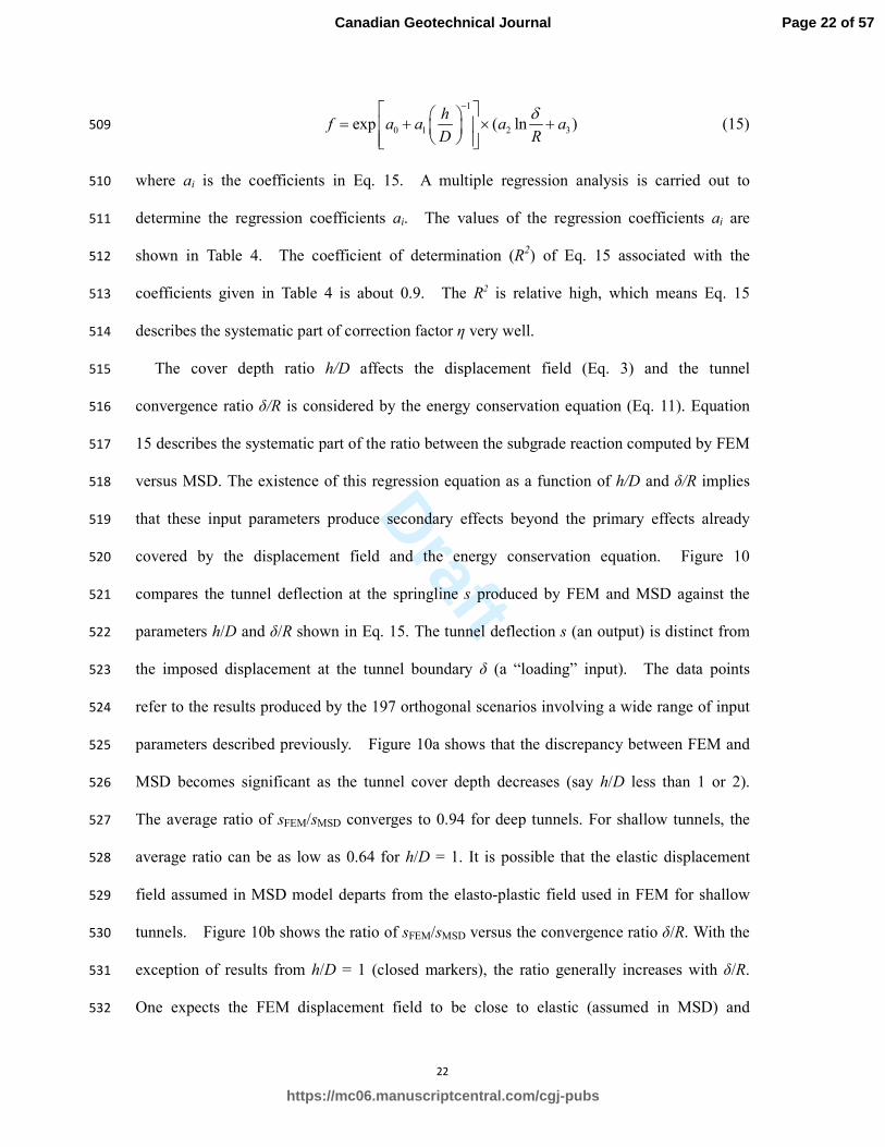
(15) 509

where ai is the coefficients in Eq. 15. A multiple regression analysis is carried out to 510

determine the regression coefficients ai. The values of the regression coefficients ai are 511

shown in Table 4. The coefficient of determination (R2) of Eq. 15 associated with the 512

coefficients given in Table 4 is about 0.9. The R2 is relative high, which means Eq. 15 513

describes the systematic part of correction factor η very well. 514

The cover depth ratio h/D affects the displacement field (Eq. 3) and the tunnel 515

convergence ratio δ/R is considered by the energy conservation equation (Eq. 11). Equation 516

15 describes the systematic part of the ratio between the subgrade reaction computed by FEM 517

versus MSD. The existence of this regression equation as a function of h/D and δ/R implies 518

that these input parameters produce secondary effects beyond the primary effects already 519

covered by the displacement field and the energy conservation equation. Figure 10 520

compares the tunnel deflection at the springline s produced by FEM and MSD against the 521

parameters h/D and δ/R shown in Eq. 15. The tunnel deflection s (an output) is distinct from 522

the imposed displacement at the tunnel boundary δ (a “loading” input). The data points 523

refer to the results produced by the 197 orthogonal scenarios involving a wide range of input 524

parameters described previously. Figure 10a shows that the discrepancy between FEM and 525

MSD becomes significant as the tunnel cover depth decreases (say h/D less than 1 or 2). 526

The average ratio of sFEM/sMSD converges to 0.94 for deep tunnels. For shallow tunnels, the 527

average ratio can be as low as 0.64 for h/D = 1. It is possible that the elastic displacement 528

field assumed in MSD model departs from the elasto-plastic field used in FEM for shallow 529

tunnels. Figure 10b shows the ratio of sFEM/sMSD versus the convergence ratio δ/R. With the 530

exception of results from h/D = 1 (closed markers), the ratio generally increases with δ/R. 531

One expects the FEM displacement field to be close to elastic (assumed in MSD) and 532

Page 22 of 57



Draft

23

therefore sFEM/sMSD ≈ 1 for small “loading” δ/R. However, this is not the trend shown in Fig. 533

10b. This may imply that there are other reasons besides the elastic displacement field 534

assumption in MSD, such as the lack of a soil unload-reload modulus in the stress-strain 535

curve for MSD and the averaging strength assumption in Eq. 6. The physical reasons 536

underlying Eq. 15 were not systematically studied in this paper. 537

The residual of the regression equation f, denoted as η*, should be the random part of the 538

correction factor η. 539

*fη η= × (16) 540

The residual η* is also plotted against the four parameters in Fig. 9 (denoted by hollow dots in 541

each figure). It is clear that the residual η* is not correlated to any input parameter, 542

particularly to h/D and δ/R, and it is appropriate to model it as a random variable. The 543

histogram of calculated residual η* is plotted in Fig. 11 (grey bars). The residual η

* is 544

observed to be lognormally distributed. The mean of residual η* is equal to 1.00 and the 545

COV is about 0.05, which suggest the precision of the proposed nonlinear solution of pk_MSD 546

could be further improved if Eq. 16 is adopted. In summary, the analytical MSD solution of 547

pk under the oval deformation mode can be as good as the corresponding FEM solution when 548

it is corrected as follows: 549

( )*

, *

0 2cos 2

u mob sArea

k

D

s dAp f

dsπ

ε δη

δ θ

⋅= × ×∫

∫ (17) 550

The only marginal cost is the model uncertainty η*, the associated COV of 0.05 is negligible 551

for all practical purposes within the geotechnical context. The proposal in this paper is to 552

modify the original MSD subgrade reaction (pk_MSD) by the regression function f. Figure 8 553

also plots the modified MSD subgrade reaction (f × pk_MSD) against the pk_FEM, denoted by the 554

solid circular dots. It is clear from Fig. 8 that the discrepancy between the pk_MSD and the 555

pk_FEM is reduced in particular at a large magnitude of pk. The range between upper and 556

Page 23 of 57



Draft

24

lower bound limits for η* has narrowed down to a maximum of 1.11 and a minimum of 0.85. 557

The same characterization procedure is carried out for the uniform deformation mode. 558

The regression equation f is derived by using 146 orthogonally designed numerical cases. 559

The analytical MSD solution of pk for the uniform deformation mode can be as good as the 560

corresponding FEM solution when it is corrected as follows: 561

( ) ( )*

1, *

0 0 1 2expu mob s

Areak

D

s dA hp b b b

RDdsπ

εη

−⋅ ∆ ∆= ⋅ + + ⋅ ∆

∫∫

(18)

562

The coefficients bi in the correlation function f are also given in Table 4. The original 563

correction factor η has a mean of 1.08 with a COV at 0.15. However, by removing the 564

dependency on input parameters using the regression equation f, the residual η* can be 565

modeled as a lognormally distributed random variable with a mean of 1.00 and a COV of 566

0.07. 567

Application Example 568

The proposed nonlinear solution of subgrade reaction pk for tunnel lining design is applied 569

to a field case reported by Huang and Zhang (2016). The site of this case located in 570

southeast part of Shanghai in China. A running metro tunnel with a diameter of 6.2m and a 571

wall thickness of 0.35m was buried 16.4m below the initial ground surface. A sectional 572

profile is shown in Fig. 12. Unfortunately, 360 lining rings of this tunnel has been subjected 573

to an unexpected ground surcharge due to soil dumping during daily metro operation. The 574

dumped soil has a height H ranging from 1.7m to 7m (shaded area in Fig. 12) causing 575

extreme surcharge loads from 30kPa to 120kPa. The design level for surcharge is 20kPa, 576

which is much smaller than this accidental surcharge. Hence, performance of the segmental 577

lining experienced a severe disruption as many of structural defects could be observed on site 578

(Huang and Zhang 2016). In this circumstance, the structural loads in the segmental lining 579

can be re-calculated to better understand the structural behavior and performance robustness 580

Page 24 of 57



Draft

25

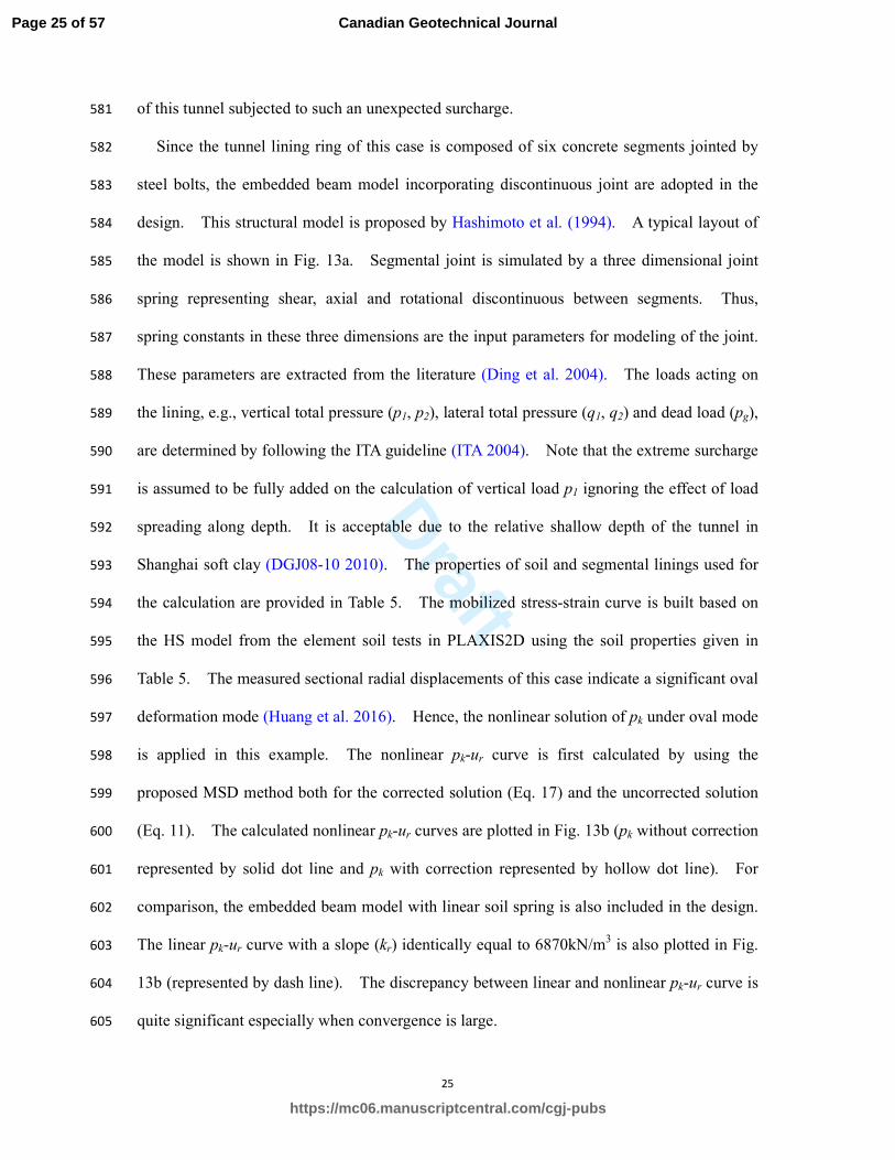
of this tunnel subjected to such an unexpected surcharge. 581

Since the tunnel lining ring of this case is composed of six concrete segments jointed by 582

steel bolts, the embedded beam model incorporating discontinuous joint are adopted in the 583

design. This structural model is proposed by Hashimoto et al. (1994). A typical layout of 584

the model is shown in Fig. 13a. Segmental joint is simulated by a three dimensional joint 585

spring representing shear, axial and rotational discontinuous between segments. Thus, 586

spring constants in these three dimensions are the input parameters for modeling of the joint. 587

These parameters are extracted from the literature (Ding et al. 2004). The loads acting on 588

the lining, e.g., vertical total pressure (p1, p2), lateral total pressure (q1, q2) and dead load (pg), 589

are determined by following the ITA guideline (ITA 2004). Note that the extreme surcharge 590

is assumed to be fully added on the calculation of vertical load p1 ignoring the effect of load 591

spreading along depth. It is acceptable due to the relative shallow depth of the tunnel in 592

Shanghai soft clay (DGJ08-10 2010). The properties of soil and segmental linings used for 593

the calculation are provided in Table 5. The mobilized stress-strain curve is built based on 594

the HS model from the element soil tests in PLAXIS2D using the soil properties given in 595

Table 5. The measured sectional radial displacements of this case indicate a significant oval 596

deformation mode (Huang et al. 2016). Hence, the nonlinear solution of pk under oval mode 597

is applied in this example. The nonlinear pk-ur curve is first calculated by using the 598

proposed MSD method both for the corrected solution (Eq. 17) and the uncorrected solution 599

(Eq. 11). The calculated nonlinear pk-ur curves are plotted in Fig. 13b (pk without correction 600

represented by solid dot line and pk with correction represented by hollow dot line). For 601

comparison, the embedded beam model with linear soil spring is also included in the design. 602

The linear pk-ur curve with a slope (kr) identically equal to 6870kN/m3 is also plotted in Fig. 603

13b (represented by dash line). The discrepancy between linear and nonlinear pk-ur curve is 604

quite significant especially when convergence is large. 605

Page 25 of 57



Draft

26

The structural responses of tunnel to the extreme surcharge are also analyzed by finite 606

element method using the PLAXIS2D code. The finite element mesh corresponding to this 607

case is illustrated in Fig. 14. Only half of the model is simulated assuming that the 608

surcharge is also distributed symmetrically with the vertical axis of metro tunnel. This 609

assumption generally agrees well with the field condition, as shown in Fig. 12. The mesh 610

has a width of 200m and a depth of 120m. The HS model is used to simulate the soil 611

behavior, and the elastic model is used to simulate the lining behavior. Input parameters for 612

these two models are shown in Table. 5. The joint between two segment linings is simulated 613

by a continuous rotation spring, as shown in the insert in Fig. 14, with a rotation stiffness 614

equal to that of the embedded beam spring model given in Table 5. Compared to the 615

embedded beam spring model, it should be noted that the shear and axial discontinuity have 616

not been simulated in this PLAXIS2D model. The stress reduction method, also named as 617

β-method, is adopted to simulate the installation of tunnel lining in numerical analysis 618

(Möller and Vermeer 2008). A reduction factor β equal to 0.25 is selected to match the 619

typical volume loss at 0.5% commonly encountered in tunneling practice in Shanghai (Ding 620

et al. 2004). The extreme surcharge above the ground surface is simulated by line load with 621

a same distribution range as that in the field. The load levels for surcharge are set 622

equivalent to the height of dumped soils from 2m to 8m. Hence, for this design example, 623

the tunnel convergence, bending moment and axial forces are calculated by four design 624

models, namely embedded beam with the corrected nonlinear soil spring model (nonlinear 625

corrected in short), embedded beam with the uncorrected nonlinear soil spring model 626

(nonlinear uncorrected in short), the embedded beam with linear soil spring model (linear 627

model) and the FEM model. 628

Figure 15 plots the calculated tunnel convergence δ at crown by using four design models 629

mentioned previously. The in-situ tunnel convergence at the crown for 360 rings also has 630

Page 26 of 57



Draft

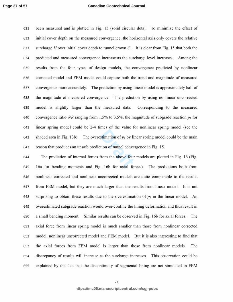
27

been measured and is plotted in Fig. 15 (solid circular dots). To minimize the effect of 631

initial cover depth on the measured convergence, the horizontal axis only covers the relative 632

surcharge H over initial cover depth to tunnel crown C. It is clear from Fig. 15 that both the 633

predicted and measured convergence increase as the surcharge level increases. Among the 634

results from the four types of design models, the convergence predicted by nonlinear 635

corrected model and FEM model could capture both the trend and magnitude of measured 636

convergence more accurately. The prediction by using linear model is approximately half of 637

the magnitude of measured convergence. The prediction by using nonlinear uncorrected 638

model is slightly larger than the measured data. Corresponding to the measured 639

convergence ratio δ/R ranging from 1.5% to 3.5%, the magnitude of subgrade reaction pk for 640

linear spring model could be 2-4 times of the value for nonlinear spring model (see the 641

shaded area in Fig. 13b). The overestimation of pk by linear spring model could be the main 642

reason that produces an unsafe prediction of tunnel convergence in Fig. 15. 643

The prediction of internal forces from the above four models are plotted in Fig. 16 (Fig. 644

16a for bending moments and Fig. 16b for axial forces). The predictions both from 645

nonlinear corrected and nonlinear uncorrected models are quite comparable to the results 646

from FEM model, but they are much larger than the results from linear model. It is not 647

surprising to obtain these results due to the overestimation of pk in the linear model. An 648

overestimated subgrade reaction would over-confine the lining deformation and thus result in 649

a small bending moment. Similar results can be observed in Fig. 16b for axial forces. The 650

axial force from linear spring model is much smaller than those from nonlinear corrected 651

model, nonlinear uncorrected model and FEM model. But it is also interesting to find that 652

the axial forces from FEM model is larger than those from nonlinear models. The 653

discrepancy of results will increase as the surcharge increases. This observation could be 654

explained by the fact that the discontinuity of segmental lining are not simulated in FEM 655

Page 27 of 57



Draft

28

model as mentioned previously. A joint model with shear and axial discontinuity would 656

absorb some of the shear and axial forces. Hence, the axial forces in the segmental lining 657

would be smaller compared to those results produced by a joint model with rotational 658

discontinuity only. Similar numerical results could also be observed in the paper elsewhere 659

(Ding et al. 2004). By comparing to the measured axial forces, the discontinued model for 660

segmental lining could predict the results much better than the conventional continuous FEM 661

model does. To sum up from Fig. 16, it is clear that a nonlinear subgrade reaction can be 662

important when the tunnel convergence is large. 663

Conclusion 664

In the practical application of embedded beam model for structural design of tunnels, the 665

soil spring is always regarded to be linear elastic. This could hardly match the reality of 666

significant nonlinear properties of soils on site. To solve this problem, this paper has 667

presented an analytical nonlinear solutions of subgrade reaction-displacement (pk-ur) curve by 668

using the mobilized strength design (MSD) method. Two typical deformation modes for 669

soil-lining interaction, i.e., uniform and oval shape functions, are used to calculate the energy 670

loss of ground movement induced by subgrade reaction. With the concept of nonlinearly 671

mobilized shear strength with engineering shear strain by averaging the curves both from 672

compression test and extension test, the subgrade reaction pk is thus obtained via the energy 673

conservation in the mobilized undrained clays. 674

The proposed nonlinear solution of pk varying with tunnel convergence (∆ or δ) is 675

successfully validated by a rigorous 2D FEM analysis with the Hardening soil (HS) model. 676

From the statistical point of view, the subgrade reaction pk from FEM analysis could be 677

predicted by the pk from MSD analysis multiplying a correction factor η of 1.02. However, 678

the η is correlated with the input parameters. If the systematic correlation characterized by a 679

regressed function f is removed in the correction factor (η*=η/f), the bias of proposed 680

Page 28 of 57



Draft

29

nonlinear model of pk_MSD compared to FEM result pk_FEM could be further reduced to a 681

residual η*. The residual η

* could be a lognormally distributed random variable with a mean 682

of 1.00 and a COV of 0.05 for oval mode and with a mean of 1.00 and a COV of 0.07 for 683

uniform mode, which are negligible for all practical purposes within the geotechnical context. 684

As shown in the application example at the end of this paper, the merit of nonlinear 685

solution of pk should be greatly appreciated when tunnel has a large deformation. The 686

prediction of convergence from nonlinear solution of pk has a very well agreements with 687

measured data and FEM model in this example. However, the magnitude of pk from linear 688

solution could be overestimated by 2-4 times the value from nonlinear solution, resulting in a 689

significant underestimation of the predicted tunnel convergence and inner forces by 2-4 times. 690

Hence, the proposed nonlinear solution of pk should be helpful in the structural design of 691

tunnel lining especially for the case that soil nonlinear behavior is mobilized significantly. 692

However, it should be noted that the proposed nonlinear solution of pk is largely based on 693

either the uniform mode or the oval mode. It also has been found in this paper that the value 694

of pk for oval shape could be 1.5-2 times the value for uniform shape. In other words, a 695

pre-judgement might be made before the application of proposed method in that the dominant 696

deformation mode should be selected. Based on the application example, the oval 697

deformation mode appears to agree with the measured data. This is the cost of analytical 698

solution by using MSD compared to the purely numerical analysis. Furthermore, soil 699

shearing may occur before the installation of the tunnel lining, resulting in a possible 700

reduction in soil strength among others. This aspect and other construction aspects that could 701

affect the determination of internal forces in the lining are not considered in this paper. 702

Acknowledgement: 703

This study is funded by the Natural Science Foundation Committee Program (51538009, 704

51608380), the Shanghai Science and Technology Committee Research Funding Program 705

Page 29 of 57



Draft

30

(15220721600), and the Ministry of Transport Construction Technology Project 706

(2013318J11300). Their support is gratefully acknowledged. 707

708

Reference 709

Arnau, O., and Molins, C. 2011. Experimental and analytical study of the structural response 710

of segmental tunnel linings based on an in situ loading test. Part 2: Numerical simulation. 711

Tunnel. Under. Space. Tech. 26(6): 778-788. doi: 10.1016/j.tust.2011.04.005. 712

Bolton, M.D., and Powrie, W. 1988. Behavior of diaphragm walls in clay prior to collapse. 713

Géotechnique 38(2): 167-189. doi: http://dx.doi.org/10.1680/geot.1988.38.2.167. 714

Bolton, M.D., Powrie, W., and Symons, I.F. 1990. The design of stiff in-situ walls retaining 715

overconsolidated clay: Part I, short term behaviour. Ground Engineering 23(1): 34-39. 716

Bransby, M.F. 1999. Selection of p-y curves for the design of single laterally loaded piles. Int. 717

J. Numer. Anal. Methods Geomech. 23(15): 1909-1926. doi: 718

10.1002/(sici)1096-9853(19991225)23:15<1909::aid-nag26>3.0.co;2-l. 719

Brinkgreve, R.B.J., Broere, W., and Waterman, D. 2006. Plaxis, Finite element code for soil 720

and rock analyses, users manual. CRC Press / Balkema, Delft, Netherlands. 721

BTS. 2004. Tunnel Lining Design Guide. Thomas Telford Limited, London. p. 184. 722

DGJ08-10. 2010. Shanghai foundation design code (DGJ08-11-10). Shanghai Construction 723

Committee, Shanghai. 724

Ding, W.Q., Yue, Z.Q., Tham, L.G., Zhu, H.H., Lee, C.F., and Hashimoto, T. 2004. Analysis 725

of shield tunnel. Int. J. Numer. Anal. Methods Geomech. 28(1): 57-91. doi: 726

10.1002/nag.327. 727

Do, N.-A., Dias, D., Oreste, P., and Djeran-Maigre, I. 2013. The behaviour of the segmental 728

tunnel lining studied by the hyperstatic reaction method. Europ. J. Environ. Civil 729

Eng.(ahead-of-print): 1-22. 730

Do, N.A., Dias, D., Oreste, P., and Djeran-Maigre, I. 2014. A new numerical approach to the 731

hyperstatic reaction method for segmental tunnel linings. Int. J. Numer. Anal. Methods 732

Geomech. 38(15): 1617-1632. 733

GB50157. 2013. Code for design of metro. Ministry of Housing and Urban-rural 734

Development (MOHURD), PRC, Beijing, China. 735

Gong, W., Juang, C.H., Huang, H., Zhang, J., and Luo, Z. 2015. Improved analytical model 736

for circumferential behavior of jointed shield tunnels considering the longitudinal 737

Page 30 of 57



Draft

31

differential settlement. Tunnel. Under. Space. Tech. 45: 153-165. doi: 738

10.1016/j.tust.2014.10.003. 739

Hashimoto, T., Hayakawa, K., Kurihara, K., Nomoto, T., Ohtsuka, M., and Yamazaki, H. 740

1996. Some aspects of ground movement during shield tunnelling in Japan. In 741

Geotechnical Aspects of Underground Construction in Soft Ground. Edited by R. Mair and 742

M.J. Taylor. Balkema, Rotterdam, Netherland. pp. 683-688. 743

Hashimoto, T., Zhu, H.H., and Nagaya, J. 1994. A new model for simulating the behavior of 744

segments in sheild tunnel. In Proc of the 49th Annual Conference of the Japan Society for 745

Civil Engineers. 746

Huang, H.-W., and Zhang, D.-M. 2016. Resilience analysis of shield tunnel lining under 747

extreme surcharge: Characterization and field application. Tunnel. Under. Space. Tech. 51: 748

301-312. doi: http://dx.doi.org/10.1016/j.tust.2015.10.044. 749

Huang, H.W., Shao, H., Zhang, D.M., and Wang, F. 2016. Deformational responses of 750

operated shield tunnel to extreme surcharge: a case study. Struct. Infrastruct. Eng.: 1-16. 751

doi: http://dx.doi.org/10.1080/15732479.2016.1170156. 752

ITA. 2004. ITA guidelines for the desigh of shield tunnel lining. International Tunneling and 753

Underground Space Association. 754

JSCE. 2007. Standard specifications for tunneling-2006: shield tunnels. Japan Society of 755

Civil Engineers, Japan. 756

Klar, A., and Klein, B. 2014. Energy-based volume loss prediction for tunnel face 757

advancement in clays. Geotechnique 64(10): 776-786. doi: 10.1680/geot.14.P.024. 758

Klar, A., Osman, A.S., and Bolton, M. 2007. 2D and 3D upper bound solutions for tunnel 759

excavation using 'elastic' flow fields. Int. J. Numer. Anal. Meth. Geomech. 31(12): 760

1367-1374. doi: 10.1002/nag.597. 761

Koutsoftas, D.C., and Ladd, C.C. 1985. Design strengths for an offshore clay. J. Geot. Eng. 762

Div. 111(3): 337-355. 763

Lee, K.M., Hou, X.Y., Ge, X.W., and Tang, Y. 2001. An analytical solution for a jointed 764

shield-driven tunnel lining. Int. J. Numer. Anal. Methods Geomech. 25(4): 365-390. doi: 765

10.1002/nag.134. 766

Möller, S.C., and Vermeer, P.A. 2008. On numerical simulation of tunnel installation. Tunnel. 767

Under. Space. Tech. 23(4): 461-475. doi: 10.1016/j.tust.2007.08.004. 768

Mair, R.J. 1979. Centrifugal modelling of tunnel construction in soft clay. In Department of 769

Geotehnical Engineering. University of Cambridge, Cambridge. 770

Mair, R.J. 2008. Tunnelling and geotechnics: new horizons. Geotechnique 58(9): 695-736. 771

Page 31 of 57



Draft

32

doi: 10.1680/geot.2008.58.9.695. 772

Mair, R.J., Taylor, R.N., and Bracegirdle, A. 1993. Subsurface Settlement Profiles above 773

Tunnel in Clays. Geotechnique 43(2): 315-320. doi: 774

http://dx.doi.org/10.1680/geot.1993.43.2.315. 775

McGann, C.R., Arduino, P., and Mackenzie-Helnwein, P. 2011. Applicability of Conventional 776

p-y Relations to the Analysis of Piles in Laterally Spreading Soil. J. Geotech. Geoenviron. 777

Eng. 137(6): 557-567. doi: 10.1061/(asce)gt.1943-5606.0000468. 778

Nogami, T., Otani, J., Konagai, K., and Chen, H.L. 1992. Nonlinear soil-pile interaction 779

model for dynamic lateral motion. J. Geotech. Eng.-ASCE 118(1): 89-106. doi: 780

10.1061/(asce)0733-9410(1992)118:1(89). 781

Oreste, P.P. 2007. A numerical approach to the hyperstatic reaction method for the 782

dimensioning of tunnel supports. Tunnel. Under. Space. Tech. 22(2): 185-205. doi: 783

10.1016/j.tust.2006.05.002. 784

Osman, A.S., Bolton, M.D., and Mair, R.J. 2006a. Predicting 2D ground movements around 785

tunnels in undrained clay. Geotechnique 56(9): 597-604. doi: 10.1680/geot.2006.56.9.597. 786

Osman, A.S., Mair, R.J., and Bolton, M.D. 2006b. On the kinematics of 2D tunnel collapse in 787

undrained clay. Geotechnique 56(9): 585-595. doi: 10.1680/geot.2006.56.9.585. 788

Osman, A.S., White, D.J., Britto, A.M., and Bolton, M.D. 2007. Simple prediction of the 789

undrained displacement of a circular surface foundation on non-linear soil. Geotechnique 790

57(9): 729-737. doi: 10.1680/geot.2007.57.9.729. 791

Park, K.H. 2005. Analytical solution for tunnelling-induced ground movement in clays. 792

Tunnel. Under. Space. Tech. 20(3): 249-261. doi: 10.1016/j.tust.2004.08.009. 793

Peck, R.B. 1969. Deep excavations and tunnelling in soft ground. In 7th Int. Conf. Soil Mech. 794

Found. Eng., Mexico City. pp. 226-290. 795

Phoon, K.K., and Kulhawy, F.H. 2005. Characterisation of model uncertainties for laterally 796

loaded rigid drilled shafts. Geotechnique 55(1): 45-54. doi: 10.1680/geot.55.1.45.58593. 797

Phoon, K.K., and Tang, C. 2015a. Model uncertainty for the capacity of strip footings under 798

negative and general combined loading. In 12th International Conference on Applications 799

of Statistics and Probability in Civil Engineering (ICASP 12), Vancouver, Canada. 800

Phoon, K.K., and Tang, C. 2015b. Model uncertainty for the capacity of strip footings under 801

positive combined loading. Geotechnical Special Publication: Honoring Wilson. H. Tang. 802

Pinto, F., and Whittle, A.J. 2014. Ground movements due to shallow tunnels in soft ground. I: 803

analytical solutions. J. Geotech. Geoenviron. Eng. 140(4): 04013040. doi: 804

10.1061/(asce)gt.1943-5606.0000948. 805

Page 32 of 57



Draft

33

Pinto, F., Zymnis, D.M., and Whittle, A.J. 2014. Ground Movements due to Shallow Tunnels 806

in Soft Ground. II: Analytical Interpretation and Prediction. J. Geotech. Geoenviron. Eng. 807

140(4): 04013041. doi: 10.1061/(asce)gt.1943-5606.0000947. 808

Sagaseta, C. 1987. Analysis of undraind soil deformation due to ground loss. Géotechnique 809

37(3): 301-320. 810

Seneviratne, H.N. 1979. Deformations and pore pressure variations around shallow tunnels in 811

soft clay. University of Cambridge, Cambridge. 812

Shen, S.L., Wu, H.N., Cui, Y.J., and Yin, Z.Y. 2014. Long-term settlement behaviour of metro 813

tunnels in the soft deposits of Shanghai. Tunnel. Under. Space. Tech. 40: 309-323. doi: 814

10.1016/j.tust.2013.10.013. 815

Standing, J.R., and Selemetas, D. 2013. Greenfield ground response to EPBM tunnelling in 816

London Clay. Geotechnique 63(12): 989-1007. doi: 10.1680/geot.12.P.154. 817

Tang, C., and Phoon, K.K. 2016a. Model uncertainty of cylindrical shear method for 818

calculating the uplift capacity of helical anchors in clay. Engineering Geology 207: 14-23. 819

doi: 10.1016/j.enggeo.2016.04.009. 820

Tang, C., and Phoon, K.K. 2016b. Model uncertainty of Eurocode 7 approach for the bearing 821

capacity of circular footings on dense sand. Int. J. Geomech.: 04016069. doi: 822

10.1061/(ASCE)GM.1943-5622.0000737, 04016069. 823

Tang, C., and Phoon, K.K. 2017. Model uncertainty for predicting the bearing capacity of 824

sand overlying clay. Int. J. Geomech. 17(7): 04017015. 825

Taylor, R.N. 1998. Modelling of tunnel behaviour. Proc. Inst. Civil Eng.-Geotech. Eng. 826

131(3): 127-132. doi: http://dx.doi.org/10.1680/igeng.1998.30467. 827

Timoshenko, S.P., and Goodier, J.N. 1970. Theory of Elasticity. Mc-Graw-Hill, New York. 828

Verruijt, A., and Booker, J.R. 1996. Surface settlements due to deformation of a tunnel in an 829

elastic half plane. Geotechnique 46(4): 753-756. 830

Verruijt, A. 1997. A complex variable solution for a deforming circular tunnel in an elastic 831

half-plane. International Journal for Numerical and Analytical Methods in Geomechanics 832

21(2): 77-89. 833

Wood, M. 1975. The circular tunnel in elastic ground. Géotechnique 25(1): 115-127. 834

Yuan, Y., Bai, Y., and Liu, J. 2012. Assessment service state of tunnel structure. Tunnel. 835

Under. Space. Tech. 27(1): 72-85. doi: 10.1016/j.tust.2011.07.002. 836

Zhang, D.M., Huang, H.W., Phoon, K.K., and Hu, Q.F. 2013. Effects of soil-lining 837

interactions on radial subgrade modulus for tunnel design. In The Twenty-Sixth 838

KKHTCNN Symposium on Civil Engineering. Edited by K.K. Phoon, Singapore. 839

Page 33 of 57



Draft

34

Zhang, D.M., Huang, H.W., Phoon, K.K., and Hu, Q.F. 2014. A Modified Solution of Radial 840

Subgrade Modulus for a Circular Tunnel in Elastic Ground. Soils and Foundations 54(2): 841

225-232. doi: http://dx.doi.org/10.1016/j.sandf.2014.02.012. 842

Zhang, D.M., Phoon, K.K., Huang, H.W., and Hu, Q.F. 2015. Characterization of Model 843

Uncertainty for Cantilever Deflections in Undrained Clay. Journal of Geotechnical and 844

Geoenvironmental Engineering 141(1): 04014088. doi: 845

10.1061/(asce)gt.1943-5606.0001205. 846

847

848

Page 34 of 57



Draft

35

849

Captions for tables and figures 850

Tables: 851

Table 1 Input parameters for HS model used in the validation (modified after data from 852

Zhang et al. 2015) 853

Table 2 Summary of statistics for correction factors and FEM (or FELA) model factor for 854

different geotechnical systems 855

Table 3 Parameters and Their Ranges of Values used in the Numerical Simulations 856

Table 4 Best regressed coefficient ai for systematic part f in correction factor η 857

Table 5 Input parameters for the design example (modified after data from Ding et al. 2004; 858

Huang and Zhang 2016). 859

860

Figures: 861

Figure 1 Deformation modes for tunnel lining: a) uniform; and b) oval. 862

Figure 2 Uniform mode for soils in semi-infinite space: a) contour lines for ground movement 863

and b) directions of principle strain 864

Figure 3 Oval mode for soils in semi-infinite space: a) contour lines for ground movement 865

and b) directions of principle strain 866

Figure 4 Finite element model used for verification of Eqs. 9 and 11: a) a typical mesh of half 867

model; b) Stress boundary condition under uniform mode; and c) stress boundary condition 868

under oval mode 869

Figure 5 Typical stress-strain curves of HS model used for the validation under two different 870

test conditions: 1) dash line for PSE; 2) solid line for PSC; and 3) dot-dash line for average of 871

PSE and PSC 872

Figure 6 Comparison of pk0 between MSD and FEM under uniform mode shape 873

Figure 7 Comparison of pk0 between MSD and FEM under oval mode shape 874

Page 35 of 57



Draft

36

Figure 8 Comparison of pk0 calculated by MSD with the results from FEM for the 875

orthogonally designed 197 cases in the validation: a) grey square dots for original MSD using 876

Eq. 11; b) black circular dots for corrected MSD results 877

Figure. 9 Correlation of calculated correction factor with input parameters in MSD: a) cover 878

depth ratio h/D; b) shear strength ratio su/σv’; c) unload-reload modulus ratio Eur/su; d) 879

convergence ratio δ/R 880

Figure 10 Comparison of tunnel deflection at the springline between FEM and MSD 881

(sFEM/sMSD) with: a) cover depth ratio h/D; b) convergence ratio δ/R 882

Figure 11 Histogram for correction factor from 197 numerical cases. 883

Figure 12 Sectional profile of the design example. 884

Figure 13 Nonlinear embedded beam spring with joint model and FEM analysis with 885

PLAIXS for design example: a) spring model layout; and b) nonlinear pk-ur curve for the 886

design. 887

Figure. 14 Element mesh in FEM analysis for the design example. 888

Figure. 15 Comparison of predicted tunnel deformation from different design model with 889

measured data; Note: measured data after (Huang and Zhang 2016). 890

Figure 16 Comparison of the predicted internal forces from different design models between 891

linear subgrade reaction and nonlinear subgrade reaction model: a) bending moment; and b) 892

axial force. 893

894

Page 36 of 57



Draft

1

Table 1 Input parameters for HS model used in the validation (modified after data from

Zhang et al. (2015))

Model Parameter (Unit) Value

General

Reference vertical earth pressure pref (kPa) 200

Soil unit weight γ (kN/m3) 18

Soil initial void ratio e0 1

HS

Soil secant stiffness in standard triaxial test E50 (kPa) 9800

Soil tangent stiffness for primary oedometer loading Eoed (kPa) 7840

Soil unloading-reloading stiffness Eur (kPa) 29400

Soil undrained shear strength su (kPa) 80

Page 37 of 57



Draft

2

Table 2 Summary of statistics for correction factors and FEM (or FELA) model factor for

different geotechnical systems

Problem η(a)

η*(b)

εFEM or εFELA (c)

N(d)

mean COV mean COV mean COV

Lateral deflection at top of cantilever wall

(MSD method) (Zhang et al., 2015) 1.01 0.47 1.01 0.18 1.01 0.18 59

Strip footings on sand under positive

combined loading (Phoon and Tang 2015a) 1.65 0.22 1.03 0.09 1.01 0.06 120

Strip footings on sand under negative

combined loading (Phoon and Tang 2015b) 2.00 0.24 1.06 0.09 1.01 0.06 72

Strip footings on sand under general

combined loading (Phoon and Tang 2015b) 2.00 0.25 1.04 0.09 1.01 0.09 192

Helical anchors in clay under tension

loading (Tang and Phoon 2017) 1.37 0.26 0.98 0.14 0.95 0.08 78

Circular footings on dense sand (Tang &

Phoon 2016a) 1.18 0.32 1.02 0.11 1.00 0.10 26

Bearing capacity of dense sand overlying

clay (punching shear method) (Tang and

Phoon 2016b)

2.63 0.31 1.01 0.12 1.01 0.11 62


clay (load spread method tanαp=1/3) (Tang

and Phoon 2016b)

1.83 0.30 1.01 0.11 1.01 0.11 62


clay (load spread method tanαp=1/5) (Tang

and Phoon 2016b)

2.32 0.33 1.02 0.11 1.01 0.11 62

Note:

a) η = correction factor

b) η*=residual part of the correction factor η, namely, η

* = η/f.

c) εFEM (or εFELA) = model factor of finite element method analysis or finite element limit analysis,

defined as εFEM = Qm/QC_FEM (or εFELA = Qm/QC_FELA), where Qm=measured data.

d) N=number of measured data for field cases and model tests.

Page 38 of 57



Draft

3

Table 3 Parameters and Their Ranges of Values used in the Numerical Simulations

Parameters Ranges of Values

h/D 1.00 – 5.00

su/σv’ 0.30 – 0.70

Eur/su 200.00 – 900.00

δ/R (∆/R) (%) 0.001 – 3.000

Page 39 of 57



Draft

4

Table 4 Best regressed coefficient ai for systematic part f in correction factor η

Oval mode Uniform mode

Coefficient Value Coefficient Value

a0 0.172 b0 -0.109

a1 -0.361 b1 0.0404

a2 0.0591 b2 0.00520

a3 1.03

R2 0.90 R

2 0.91

Page 40 of 57



Draft

5

Table 5 Input parameters for the design example (modified after data from Ding et al. 2004;

Huang and Zhang 2016).

Design objective Design input parameter Value

Tunnel Lining

Outer-diameter D (m)

Wall thickness t (m)

Elastic modulus E (kPa)

Joint compressive stiffness kn_joint (kN/m)

Joint shear stiffness ks_joint (kN/m)

Joint rotate stiffness kr_joint: (kN/rad)

6.2

0.35

34.5×106

1×104

8×104

3.5×104

Soil

Cover depth to tunnel crown C (m)

Soil unit weight γ (kN/m3)

Coefficient of earth pressure at-rest K0

Surcharge at ground surface H (m)

Soil undrained shear strength su (MPa)

Soil unloading-reloading modulus Eur (MPa)

16.4

16.7

0.54

1.7 – 7

46

21.3

Page 41 of 57



Draft

1

∆

∆∆

∆

δ

δδ

δ

θ

(a) (b)

Figure 1 Deformation modes for tunnel lining: a) uniform; and b) oval.

Page 42 of 57



Draft

2

u=50%∆

A 2 2

x zu u u= +

R

z

xux

uz

h

pkr

∞

∞∞

(a)

Plane-strain Extension(PSE)

PSE

Plane-strain Compression

(PSC)PSC Tunnel

(b)

Figure 2 Uniform mode for soils in semi-infinite space: a) contour lines for ground movement

and b) directions of principle strain

Page 43 of 57



Draft

3

pk

u=50%∆

A

2 2

x zu u u= +

R

z

xux

uz

h

r

∞

∞ ∞

(a)

PSE

PSE

PSEPSE

Tunnel

(b)

Figure 3 Oval mode for soils in semi-infinite space: a) contour lines for ground movement

and b) directions of principle strain

Page 44 of 57



Draft

4

Half width = 200m

Depth = 120m h= 25m

R = 3m

Stress boundary around tunnel perimeter(oval in this case)

Ground surface

(a)

pk

pk=pk0

e.g.

pk0=100kPa

100kPa

100kPa

100kPa

100kPa

pk=pk0cos2θ

θ

pk

e.g.

pk0=100kPa

100kPa

-100kPa -100kPa

100kPa

(b) (c)

Figure 4 Finite element model used for verification of Eqs. 9 and 11: a) a typical mesh of half

model; b) Stress boundary condition under uniform mode; and c) stress boundary condition

under oval mode.

Page 45 of 57



Draft

5

0.00

0.20

0.40

0.60

0.80

1.00

1.20

0.00E+00 2.00E-02 4.00E-02 6.00E-02 8.00E-02 1.00E-01

Mob

iliz

ed s

tren

gth

rati

o

(su

,mo

b/s

u)

Engineering shear strain (εs)

HS-extension

HS-compression

HS-Average

Figure 5 Typical stress-strain curves of HS model used for the validation under two different

test conditions: 1) dash line for PSE; 2) solid line for PSC; and 3) dot-dash line for average of

PSE and PSC

Page 46 of 57



Draft

6

0

50

100

150

0.00 0.50 1.00 1.50

Su

bgra

de

Rea

ctio

n p

k0

(kP

a)

Tunnel convergence ratio ∆/R (%)

Plaxis

MSD-HS-Average

Elastic solution

Uniform

shape

Shanghai code for SLS (0.5%)

Chinese code for SLS (0.3-0.4%)

Figure 6 Comparison of pk0 between MSD and FEM under uniform mode shape

Page 47 of 57



Draft

7

0

100

200

300

0.00 0.50 1.00 1.50

Su

bgra

de

Rea

ctio

n p

k0

(kP

a)

Tunnel convergence ratio δ/R (%)

Plaxis

MSD-HS-Average

Elastic solution

Oval shape

Shanghai code for SLS (0.5%)

Chinese code for SLS (0.3-0.4%)

Figure 7 Comparison of pk0 between MSD and FEM under oval mode shape

Page 48 of 57



Draft

8

0.50

5.00

50.00

500.00

0.50 5.00 50.00 500.00

FE

M i

np

ut

pk

(kP

a)

MSD Calculated pk (kPa)

Original MSD

Corrected MSD

45 degree line

η = 0.66

η = 1.28

η* = 1.11

η* = 0.85

η η*

mean 1.02 1.00

COV 0.15 0.05

smaple 197 197

Figure 8 Comparison of pk0 calculated by MSD with the results from FEM for the

orthogonally designed 197 validation cases under oval mode shape: a) grey square dots for

original MSD using Eq. 11; b) black circular dots for corrected MSD results

Page 49 of 57



Draft

9

0.50

0.75

1.00

1.25

0.00 1.00 2.00 3.00 4.00 5.00 6.00

Averag

ed

Co

rrecti

on

facto

r

ηa

ve

Cover depth ratio (h/D)

Correction factor

Residual of correction factor

Spearman Correlation Test

p-value = 5.00××××10-6

0.50

0.75

1.00

1.25

0.20 0.30 0.40 0.50 0.60 0.70 0.80

Avera

ged

Corre

ctio

n f

act

or

ηav

e

Undrained shear strength ratio (su/σv')

Correction factor

Residual of correction factorSpearman Correlation Test

p-value = 0.38

(a) (b)

0.50

0.75

1.00

1.25

100 300 500 700 900

Aver

ag

ed C

orr

ecti

on

fact

or

ηa

ve

Unload-reload modulus ratio (Eur/sv)

Correction factor



p-value = 0.76

0.50

0.75

1.00

1.25

1.50

1.00E-03 1.00E-02 1.00E-01 1.00E+00 1.00E+01

Co

rre

cti

on

facto

r η

Oval convergence ratio δ/R (%)

Correction factor



p-value = 0.00

(c) (d)

Figure. 9 Correlation of calculated correction factor with input parameters in MSD under oval

mode shape: a) cover depth ratio h/D; b) shear strength ratio su/σv’; c) unload-reload modulus

ratio Eur/su; d) convergence ratio δ/R

Page 50 of 57



Draft

10

0.00

0.20

0.40

0.60

0.80

1.00

1.20

1 2 3 4 5

s FE

M/s

MS

D

h/D

s

(a)

0.00

0.20

0.40

0.60

0.80

1.00

1.20

1.0E-04 1.0E-03 1.0E-02 1.0E-01 1.0E+00

s FE

M/s

MS

D

δ/R (%)

s

Range in practice

(b)

Figure 10 Comparison of tunnel deflection at the springline between FEM and MSD

(sFEM/sMSD) with: a) cover depth ratio h/D; b) convergence ratio δ/R

Page 51 of 57



Draft

11

0.00

0.10

0.20

0.30

0.40

0.50

0.50 0.60 0.70 0.80 0.90 1.00 1.10 1.20 1.30 1.40 1.50

Rela

tiv

e F

req

uen

cy

Correction factor

Histogram for η*

Histogram for η

Lognormal PDF for η*

η η*

mean 1.02 1.00

COV 0.15 0.05

smaple 197 197

Figure 11 Histogram for correction factor from 197 numerical cases under oval mode shape

Page 52 of 57



Draft

12

Shanghai Metro

Tunnel

D=6.2m

Elevation of surcharge

Initial ground surface

15

7

-1

-9

-17

-25

-33

-41

Elevation

Shanghai Soft Clay

Surcharge

C=

16

.4m

H

Figure 12 Sectional profile of the design example

Page 53 of 57



Draft

13

p1

p2

q1

q2 q2

q1

pg

Soil Spring

Tunnel Lining

r0

Segment joint

kr_joint

kn_joint

ks_joint

(a)

0.00

200.00

400.00

600.00

800.00

0.00 1.00 2.00 3.00 4.00 5.00 6.00 7.00

Su

bg

rad

e re

act

ion

pk

(kP

a)

Tunnel convergence ratio δ/R (%)

Subgrade reaction pk-ur

curve

(b)

Figure 13 Nonlinear embedded beam spring with joint model and FEM analysis with

PLAIXS for design example: a) spring model layout; and b) nonlinear pk-ur curve for the

design.

Page 54 of 57



Draft

14

Half width = 200m

Depth = 120m

Initial ground surfaceh= 19.5m

Extreme surcharge

Rotational Spring in PLAXIS

Metro tunnel D = 6.2m

Figure. 14 Element mesh in FEM analysis for the design example

Page 55 of 57



Draft

15

0.00

2.00

4.00

6.00

0.10 0.20 0.30 0.40 0.50

Tu

nn

el c

on

ver

gen

ce r

ati

o

δ/R

(%

)

Relative surcharge level (H/C)

Measured (Zhang et al. 2016)

Designed Nonlinear Corrected

Designed Nonlinear Uncorrected

Designed Linear

PLAXIS2D

Figure. 15 Comparison of predicted tunnel deformation from different design model with

measured data; Note: measured data after (Huang and Zhang 2016)

Page 56 of 57



Draft

16

0

100

200

300

400

0.1 0.2 0.3 0.4 0.5

Ben

din

g M

om

ent

M

(kN

m)


M (Nonlinear Corrected)M (Nonlinear Uncorrected)M (Linear)M (PLAXIS)

(a)

500

700

900

1100

1300

1500

0.1 0.2 0.3 0.4 0.5

Ax

ial

Fo

rce N

(kN

)


N (Nonlinear Corrected)

N (Nonlinear Uncorrected)

N (Linear)

N (PLAXIS)

(b)

Figure 16 Comparison of the predicted internal forces from different design models between

linear subgrade reaction and nonlinear subgrade reaction model: a) bending moment; and b)

axial force

Page 57 of 57



Documents

Draft - tspace.library.utoronto.ca · Draft 2 20 Nonlinear Subgrade Reaction Solution for Circular Tunnel Lining Design Based 21 on Mobilized Strength of Undrained Clay 22 23 Abstract: