DRAFT - Axioma | Home Pages/alighningalpha...DRAFT Aligning Alpha and Risk Factors, a Panacea to Factor Alignment Problems? implied alpha,?, can still be non-zero, have overlap with

DRAFT

Axioma Research Paper

No. 38

February 22, 2012

Aligning Alpha and Risk Factors, a

Panacea to Factor Alignment Problems?

The practical issues that arise due to the interaction be-tween three principal players in any quantitative strategy,namely, the alpha model, the risk model and the constraintsare collectively referred to as Factor Alignment Problems(FAP). While the role of misaligned alpha factors in caus-ing FAP is relatively easy to understand, incorporating theimpact of constraints entails considerable analytical com-plexity that most consultants and researchers find difficultto fathom. A few of them have even gone to the extent ofsuggesting that aligning alpha and risk factors should sufficein handling FAP. We provide a solid rebuttal to this line ofthinking by demonstrating typical symptoms of FAP in op-timal portfolios generated by using completely aligned alphaand risk models. Additionally, we provide theoretical guid-ance to clarify the role of constraints in influencing FAP andillustrate how the Alpha Alignment Factor (AAF) method-ology can handle misalignment resulting from constraints,analytical complexities notwithstanding.

DRAFT

Aligning Alpha and Risk Factors, a Panacea to Factor Alignment Problems?

Aligning Alpha and Risk Factors, a Panacea toFactor Alignment Problems?

Anureet Saxena, Ph.D, CFA Christopher Martin, CAIARobert A. Stubbs, Ph.D

February 22, 2012

1 Introduction

The practical issues that arise due to the interaction between three principal players inany quantitative strategy, namely, the alpha model, the risk model and the constraints arecollectively referred to as Factor Alignment Problems (FAP). Examples of FAP include risk-underestimation of optimized portfolios, undesirable exposures to factors with hidden andunaccounted systematic risk, consistent failure in achieving ex-ante performance targets, andinability to harvest high quality alphas into above-average IR.

Despite several studies (Alford et al. (2003); Renshaw et al. (2006); Lee and Stefek (2008);Saxena and Stubbs (2010a,b); Ceria et al. (2012); Saxena and Stubbs (2011)), there is con-siderable disparity in understanding the sources of FAP. While the role of misaligned alphafactors is relatively easy to understand, incorporating the impact of constraints entails con-siderable analytical complexity that most consultants and researchers find difficult to fathom.A few of them have even gone to the extent of suggesting that aligning alpha and risk fac-tors should suffice in handling FAP. We provide a solid rebuttal to this line of thinking bydemonstrating typical symptoms of FAP in optimal portfolios generated by using completelyaligned alpha and risk models. Additionally, we provide theoretical guidance to clarify therole of constraints in influencing FAP and illustrate how the Alpha Alignment Factor (AAF)methodology can handle misalignment resulting from constraints, analytical complexitiesnotwithstanding.

The results presented in this paper are important for two reasons. One, by virtue ofrecent developments in risk model infrastructure such as the Risk Model Machine (RMM),it is now possible to surgically remove the misalignment between alpha and risk factorsby constructing custom risk models (CRM) that explicitly incorporate the alpha factors.Construction of CRM involves complete recalibration of the covariance matrix by re-runningthe cross sectional regressions, recomputing factor returns attributed to the original andcustom risk factors, and using the resulting time series of factor and residual returns tocompute the factor-factor covariance matrix and specific risks. Among other things, CRMcapture the temporal fluctuations in the volatility of alpha factors, and hence provide asophisticated means of handling misalignment arising from alphas. Unfortunately, no suchexact approach has yet been developed to handle misalignment arising from constraints which

Axioma 2

DRAFT


is usually more difficult to characterize apriori. For instance, misalignment arising fromthe turnover constraint depends on the asset trades which are determined only during theportfolio construction phase. Our results show that despite their analytical complexity, themisalignment arising from constraints is a “real” problem that compromises the efficiencyof the resulting portfolios. In other words, performance sensitive portfolio managers cannotafford to ignore risk under-estimation problems that arise due to constraints.

Second, we revisit the Alpha Alignment Factor (AAF) methodology and establish itsefficacy in handling misalignment arising from constraints. While researchers have previouslyargued about the capability of the AAF methodology to handle misalignment arising fromboth alphas and constraints, a focused empirical illustration of AAF in handling FAP arisingexclusively from constraints has been lacking until our work. To summarize, we not onlyhighlight the gravity of misalignment problems that arise due to constraints but also illustratea practical solution in the form of the AAF to circumvent them.

The rest of the paper is organized as follows. We initiate our investigation (Section 2) witha very simple strategy that has no conspicuous source of misalignment; specifically, we use anidentical set of alpha and risk factors. Despite the idyllic nature of this strategy, the resultingoptimal portfolios display the quintessential symptom of FAP, namely, downward bias in riskprediction. We investigate the source of the mentioned bias and trace it to the long-only andactive asset bound constraints; while neither of these constraints have appeared prominentlyin the alignment debate, our results show that they can introduce statistically significant biasin risk prediction. Subsequently, we extend our findings to variants of the above strategythat encompasses practical considerations such as turnover limitations, average daily volume(ADV) constraint, illiquidity motivated asset bounds, market impact function, transactioncost models, etc.

Section 3 revisits the constrained Mean Variance Optimization (MVO) model from ana-lytical perspective and dwells on the interchangeable role of alpha and constraints. Amongother things, we give a structural result to demonstrate how the orthogonal components ofboth alpha and constraints can introduce misalignment, and misguide the optimizer to takeexposure to latent systematic risk factors thus providing theoretical underpinning to resultspresented in this paper. In Section 4 we highlight the “opportunity” cost of not addressingthe misalignment between constraints and risk factors. Our results show that the ill effectsof misalignment due to constraints extend beyond the immediately visible effects such as bi-ased risk prediction, and materially impact the efficiency of the resulting portfolios. In otherwords, the latent systematic risk factors associated with constraints disorient the ability ofthe optimizer to perform optimal budget and risk allocation as justified by the risk-returncharacteristics of individual securities. As a byproduct, we show how the Alpha AlignmentFactor (AAF) approach remedies many of these problems and helps restore efficiency of theoptimal portfolio. We end the paper with some concluding remarks in Section 5.

Throughout this paper we use the words expected returns and alpha synonymously. Also,the proofs of theoretical results presented in this paper are fairly straightforward and omittedfor the sake of brevity.

Axioma 3

DRAFT


2 Misalignment from Constraints

We initiate our investigation with a very simple strategy to highlight the role of constraintsapropos FAP. We used the following long-only strategy, referred to as the base strategy, inour experiments.

maximize Expected Returns.t

Fully invested long-only portfolioActive sector exposure constraintActive industry exposure constraintActive asset bounds constraintActive Risk constraint (σ)Benchmark = S&P 600 .

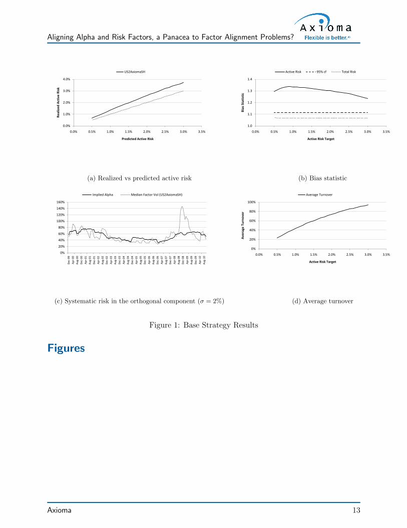
We used Axioma’s short horizon fundamental risk model (US2AxiomaSH) to define the track-ing error constraint, and an equal weighted combination of “Growth” and “Short Term Mo-mentum” factors in US2AxiomaSH to define the expected returns thus ensuring completealignment between the alpha and risk factors. The industry factors in US2AxiomaSH wereused to define the industry bound constraints whereas combinations of industry factors asdictated by GICS were used to define the sector bound constraints. We ran a monthly back-test using the above strategy in the 1998-2010 time period for σ = 0.5%, 0.6%, . . . , 3.0%.Next, we report our computational findings.

Figure 1a plots the predicted and realized active risk of the portfolios for various risk targetlevels; for the sake of comparison, we also show a dotted line that corresponds to completelyunbiased risk prediction. Figure 1b reports the same information using the concept of thebias statistic. The bias statistic is a statistical metric which is used to measure the accuracyof risk prediction; if the ex-ante risk prediction is unbiased, then the bias statistic shouldbe close to 1.0 (see Saxena and Stubbs (2010a) for more details). Several comments are inorder.

First, note the significant downward bias in risk prediction (Figure 1a); Figure 1b showsthat the bias statistics associated with active risk forecasts are significantly above the 95%confidence interval thereby confirming the statistical significance of the mentioned bias. Sec-ond, the bias statistic associated with the total risk of the portfolio was within the 95%confidence interval [0.88, 1.12]. This suggests that the risk model was able to produce un-biased forecasts for the total risk of the portfolio, and the downward bias was limited tothe active risk forecasts, a classic symptom of FAP (also see Saxena and Stubbs (2010a)).Third, by virtue of complete alignment between the alpha and risk models, it follows thatthe residual component of alpha, α⊥, that is uncorrelated with factors in the risk model isvacuous1. Among other things, this implies that penalizing the exposure of the portfolio toα⊥ will not remedy the problem. Fourth, even though α⊥ = 0, the residual component of

1Given an arbitrary factor f and a set of risk factors S = {f1, f2, . . . , fn}, the residual or orthogonalcomponent of f , denoted by f⊥, is defined to be the residual obtained by regressing f against factors in S.The portion of f , namely f − f⊥, which is explained by the risk factors in S is referred to as the spannedcomponent of f . Unless otherwise stated, we always assume that S contains all the risk factors in the riskmodel under consideration.

Axioma 4

DRAFT


implied alpha, γ⊥, can still be non-zero, have overlap with latent systematic risk factors andthus induce the optimizer to take inadvertent exposure to systematic risk factors.

One way of confirming the above hypothesis is to compute the realized systematic riskin γ⊥ and compare it with the systematic risk in a median risk factor of US2AxiomaSH.We used the augmented regression methodology described in Saxena and Stubbs (2011) tocompute the realized systematic risk in γ⊥; Figure 1c reports the timeseries of annualizedvolatility of factor returns that can be attributed to γ⊥ (σ = 2%) computed using a rolling24-period window. For the sake of comparison, we also report median systematic risk in(scaled) risk factors associated with US2AxiomaSH. Except for a brief period during the2008 crisis, the two timeseries shown in Figure 1c track each other quite consistently. Thisimplies that not only does γ⊥ have systematic risk, γ⊥ is, in fact, comparable to a medianrisk factor in US2AxiomaSH. Despite our earnest attempt to circumvent all possible sourcesof misalignment, the orthogonal component of implied alpha still manages to take exposureto latent systematic risk factors thus exposing the optimal portfolio to vagaries of FAP. Howdo we explain this phenomenon?

The answer to the above question lies in the following construction of implied alpha,

γ = α− ATπ ,

where γ denotes implied alpha, α denotes expected returns (alpha), A denotes the exposurematrix of constraints and π denotes the associated shadow prices; the relationship expressedin the above equation naturally carries over to the orthogonal components of implied alpha,alpha and constraint exposures. Since we use identical alpha and risk factors, γ⊥ is deter-mined by the orthogonal component of constraints. Furthermore, since industry and sectorbound constraints are derived from industry factors in US2AxiomaSH, the only constraintsthat have a non-trivial orthogonal component are the long-only and active asset bound con-straints given by,

hi ≥ 0 (long − only constraint)hi − bi ≥ li (active lower bound constraint)

hi − bi ≤ ui (active upper bound constraint) ;

hi and bi denote the portfolio and benchmark holding for asset i, respectively. During theprocess of portfolio construction, the optimizer determines the subset of long-only and activeasset bound constraints that would be binding at the optimal portfolio. If the set of assetscorresponding to these binding constraints have certain common aka ‘systemic’ characteristicsthen there is a possibility for the existence of latent systematic risk exposure in the resultingportfolios. We illustrate this subtle but extremely important technical point by two examples.

First, consider a Socially Responsible Investment (SRI) strategy that prohibits investmentin companies that benefit from tobacco, alcohol or gambling activities; for sake of brevity, werefer to such companies as TAG companies. Naturally optimal portfolios managed accordingto the SRI mandate would have negative active exposure to TAG stocks. If the risk modelthat is used in construction of such SRI portfolios does not have a TAG industry factor thenthe optimizer is likely to overlook the systematic component of the negative active TAGexposure resulting in unaccounted systematic risk and a downward bias in risk prediction.Note that in this case the misalignment is introduced by binding constraints that prohibit

Axioma 5

DRAFT


the ownership of TAG stocks regardless of the mutual alignment, or lack thereof, betweenthe alpha and risk factors.

Second, in the context of our base strategy, note that long-only and active asset boundconstraints are likely to be binding at assets that are either in the bottom or top decileof the alpha ranking. Such a collection of assets can have its unique characteristics andhence systematic risk exposures which are not completely captured by the risk model despiteconformity between the alpha and risk factors. In order to test this hypothesis, we conductedthe following experiment.

We derived the so-called “tail-alpha” from the alpha for the above strategy by sorting theassets by their alpha scores and setting the alpha exposure of all assets which are not presentin the top or bottom decile to zero. To put it differently, we retained the original alpha valuesfor only those assets that are most likely to yield binding active asset bound or long-onlyconstraints. Figure 2a shows the decomposition of tail alpha in terms of the spanned andorthogonal components while Figure 2b shows the realized systematic risk of the orthogonalcomponent of tail alpha computed using the augmented regression model. It is interestingto note that even though tail alpha is derived using risk factors in US2AxiomaSH, it still hasnon-trivial orthogonal component which in turn has significant latent systematic risk.

These experiments illustrate how long-only and active asset bound constraints introducemisalignment in a strategy that uses identical alpha and risk models. Next, we proceed toanalyze the marginal impact of various practical considerations on these findings. One ofthe common features of almost every quantitative strategy is a conscious attempt to controltransaction costs and other trading expenses. As show in Figure 1d, the monthly turnoverof portfolios generated using the base strategy was unreasonably high. We conducted analternative set of experiments wherein we augmented the original strategy by a turnoverconstraint that limits the monthly turnover to 18%. Figures 3a-3d report the key findingsof this experiment. Note that the qualitative nature of these results - statistically significantdownward bias in risk prediction and latent systematic risk in the orthogonal component ofimplied alpha - is similar to those obtained with the base strategy. The humped shape ofthe bias statistic graph shown in Figure 3b suggests that the bias in risk prediction initiallyincreases with increasing active risk targets and then continues to decline. The section thatfollows provides a theoretical model to explain this rather intriguing phenomenon.

Some portfolio managers (PM) prefer to optimize the trade off between expected returnsand transaction costs as a proxy for the turnover constraint. To capture the effect of misalign-ment on such strategies, we modified the objective function of the base strategy to includea transaction cost term. Figures 4a-4d report the computational results reconfirming thedownward bias and other symptoms of FAP despite complete alignment between alpha andrisk models. These two cases are particularly interesting since they show how misalignmentcan arise from trading considerations.

Another important concern while managing small-cap portfolios is excessive exposure toilliquid stocks. Markets for such stocks have limited depth, and excessive trading, measuredas a proportion of average daily volume (ADV), can significantly move the stock prices. Thereare several ways of incorporating these liquidity concerns; we discuss three such approachesbelow in the context of FAP.

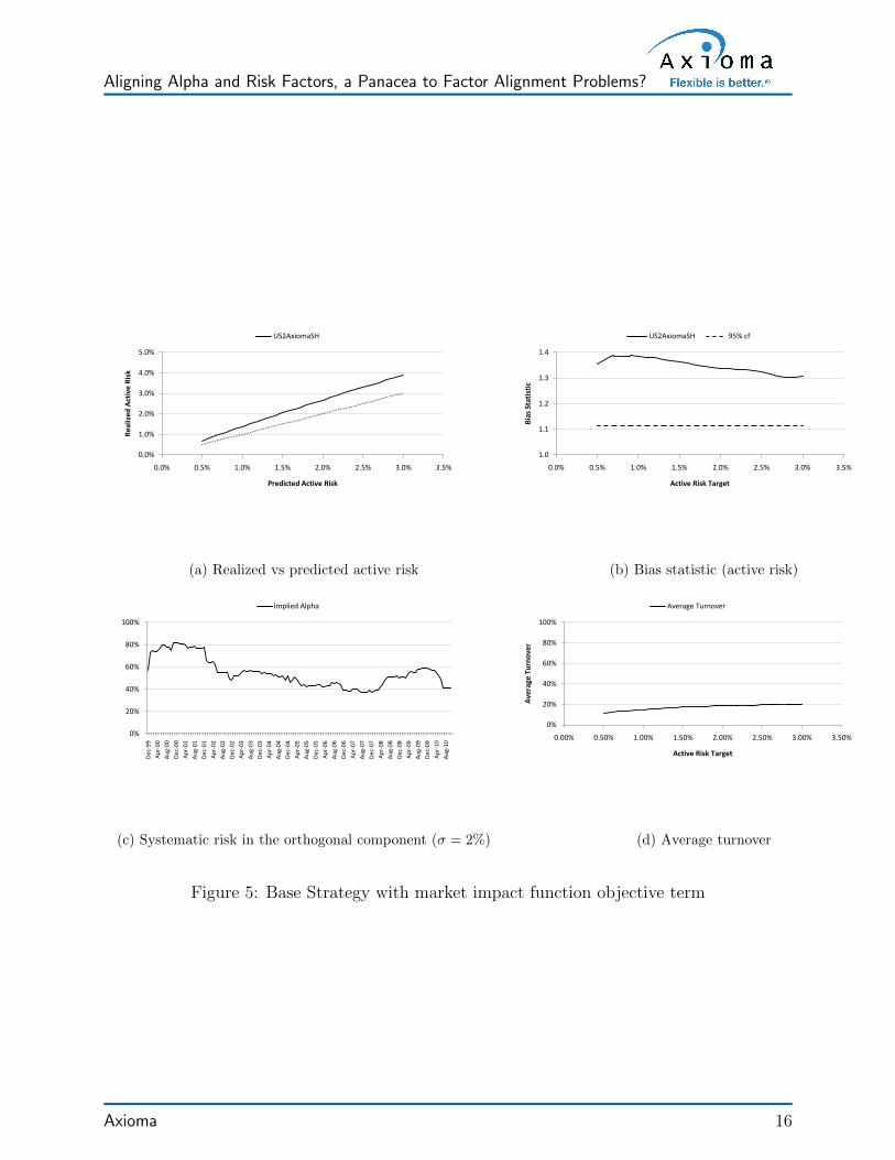
In the first set of experiments, we added a market impact function to the objectivefunction of the base strategy to capture the effect of trading induced price fluctuations.

Axioma 6

DRAFT


Figures 5a-5d report our key findings. It is interesting to note that the bias statistics in thiscase are close to 1.4 for some of the risk targets thus defying the notion that only alphascontribute to misalignment problems. A second approach to handle liquidity concerns isto add a constraint, referred to as the ADV constraint, that limits the exposure to assetswith limited average daily trading volume; Figures 6a-6d reports the results for the strategyobtained by adding the ADV constraint to the base strategy. Finally, a third approachentails modifying the active asset bounds for illiquid assets. We implemented this approachby reducing the maximum possible deviation from benchmark weights by 50% for assetswhich were in the bottommost quartile of the liquidity factor in US2AxiomaSH; Figures7a-7d report the computational results.

One may be tempted to believe that misalignment problems illustrated so far are limitedto quantitative strategies that invest exclusively in small-cap assets or use a short-horizonrisk model. We next describe a simple experiment that refutes this hypothesis. We repeatedthe above set of experiments with a variant of the base strategy obtained by making threemodifications. First, we replaced the benchmark, and hence the universe of investable assets,by S&P 500. Second, we used the medium horizon risk model (US2AxiomaMH) instead ofUS2AxiomaSH. Finally, we used the medium-term variant of the momentum factor insteadof the short-term variant to define the expected returns. Figures 8a-8d report the key results.Symptoms of FAP that we discovered in previous set of experiments are equally conspicuous inthis case too, our choice of a large-cap asset universe or a different risk model notwithstanding.

A common theme among all of these experiments is the empirical demonstration of FAPdespite using a common set of alpha and risk factors. The strategies used in these experimentswere intentionally kept simple to facilitate effortless replication; we believe that similar resultswould be obtained regardless of the choice of optimizer or risk model. The section that followsprovides a theoretical underpinning for the empirical results presented in this section.

3 Theoretical Insights

In this section, we give some theoretical results to shed light on the role of constraints inthe context of factor alignment problems. For the sake of analytical accessibility, we limitour discussion to constrained mean-variance optimization (MVO) problems with a singleconstraint. All of these results can be easily generalized to encompass several additionalconstraints.

Consider the following constrained MVO problem with a single factor exposure constraint,

max αTh− λ2hTQh

s.t.βTh ≥ β0 .

MV O(α, β) .

Let h(α, β) denote the optimal solution to MVO(α, β). Our goal is to understand the roleof the constraint βTh ≥ β0 in influencing the composition of the optimal portfolio h(α, β).In order to pursue this goal, we define two auxiliary unconstrained MVO problems, namely,

max αTh− λ2hTQh MV O(α) and

max βTh− λ2hTQh MV O(β) .

Axioma 7

DRAFT


Let h(α) and h(β) denote the optimal solutions to MVO(α) and MVO(β), respectively. Notethat if βTh(α) ≥ β0 then h(α) is also an optimal solution to MVO(α, β) thereby rendering theconstraint βTh ≥ β0 irrelevant. Thus for the purpose of our discussion we assume that h(α)violates the constraint βTh ≥ β0, and let η = β0 − βTh(α) denote the associated constraintviolation. Furthermore, without loss of generality we can assume that βTQ−1β = 1. Thetheorem that follows establishes an important link between h(α), h(β) and h(α, β).

Theorem 1. h(α, β) = h(α) + (ηλ)h(β).Theorem 1 shows that the optimal solution to MVO(α, β) is obtained by tilting the opti-

mal solution h(α) to the unconstrained problem MVO(α) in the direction h(β). Furthermore,the extent of tilting is jointly determined by the risk aversion parameter λ in MVO(α, β) andthe violation η of the constraint βTh ≥ β0 by h(α). The higher the risk aversion parameter λ,more significant is the influence of the constraint βTh ≥ β0 in determining h(α, β). Similarly,tighter constraints give rise to higher violation η and consequently have greater influence indetermining h(α, β).

Theorem 1 also provides additional insights from an alignment perspective. Note thatthe relationship expressed in Theorem 1 naturally extends to the orthogonal componentsof h(α), h(β) and h(α, β). It has been well documented in the literature (Lee and Stefek(2008); Saxena and Stubbs (2010b)) that optimal portfolios associated with unconstrainedMVO problems load up on the orthogonal component of the expected returns. For instance,if α⊥ 6= 0 (β⊥ 6= 0) then h(α) (h(β)) will have disproportionately higher exposure to α⊥(β⊥).Theorem 1 extends these findings to constrained MVO problems with an intriguing twist. Itshows that h(α, β) loads up not only on the orthogonal component of α, by virtue of the termh(α), but also on the orthogonal component of β due to the presence of the term (ηλ)h(β).Furthermore, the extent of overloading depends directly on the magnitudes of λ and η.Specifically, highly risk averse strategies that use a higher value of λ, or equivalently lowervalue of risk targets σ, are more likely to suffer from misalignment arising from constraints.Of course, if the value of λ (σ) is very large (small) then the role of constraints diminishesand the portfolio holdings start to resemble minimum variance portfolios, or the benchmarkholdings in the case of active strategies.

To summarize, the downward bias in risk prediction that arises exclusively due to thepresence of constraints should have a humped shape attaining highest values at moderaterisk target levels. This jibes well with the shapes of bias statistics charts shown in Figures 1b,3b, 4b, 5b, 6b and 7b. By similar arguments, it follows that strategies with tighter constraintsleading to higher values of the violation parameter (η) would betray similar characteristics.

Until now we have examined results that corroborate the role of constraints in the con-struction of optimal portfolios. Next we present an interesting result that reverses the rolesof alphas and constraints altogether. Consider the following MVO problem.

max βTh− 12ηhTQh

s.t.αTh ≥ α0 .

MV O(β, α) ,

where α0 = αTh(α, β). Let h(β, α) denote the optimal solution to MVO(β, α).

Theorem 2. (α− β Interchangeability Theorem) h(α, β) = h(β, α).

Axioma 8

DRAFT


Theorem 2 shows that MVO(α, β) and MVO(β, α) have identical optimal solutions. Inother words, there is nothing sacrosanct about alphas in a constrained MVO problem, and thesame optimal portfolio can be obtained by switching the role of alphas and constraints. Asan immediate corollary, it follows that the misalignment between constraints and risk factorscan have as much influence, if not more, in determining the composition of optimal holdingsas that between alpha and risk factors. Furthermore, the relative significance of misalignmentdue to alpha and constraints can be gauged by comparing the risk-aversion parameters inMVO(α, β) and MVO(β, α). Specifically, the higher the violation η, the smaller is the riskaversion parameter in MVO(β, α) and more prominent is the role of constraints. Notably,the ratio of the risk aversion parameters, namely ηλ, is precisely the amount by which h(α)is tilted towards h(β) to determine the optimal solution to MVO(α, β) (see Theorem 1).

Next we briefly discuss a solution approach, namely the Alpha Alignment Factor (AAF)methodology, to address misalignment arising from constraints. We limit our discussion tokey insights and refer the readers to Saxena and Stubbs (2010b) for further details. Sincethe focus of this paper is misalignment arising exclusively from constraints, we assume thatα⊥ = 0 in the discussion that follows. Recall that if α⊥ = 0, then the only source ofmisalignment is the orthogonal component of β. In fact, in this case it can be easily shownthat the orthogonal component of implied alpha (γ) and β⊥ point in the same direction i.e.

1‖γ⊥}

γ⊥ = 1‖β⊥}

β⊥. The AAF approach recognizes the possibility of systematic risk in theorthogonal component of implied alpha, and penalizes the exposure of the portfolio to γ⊥.In our special setting, the AAF optimization problem can be stated as,

max αTh− λ2

(hTQh+ ν (hTy)2

)s.t.

βTh ≥ β0 ,(MVO(AAF ))

where y = 1‖β⊥‖

β⊥, and ν is the systematic risk associated with y. Note that MVO(AAF )

can be obtained from MVO(α, β) by replacing the covariance matrix Q by an augmentedcovariance matrix Qy = QQ + νyyT that has an additional variance term νyyT to capturesystematic risks in portfolios by virtue of exposure to β⊥. Net we discuss some importantcharacteristics of the optimal solution, say hy, to MVO(AAF ), and compare them with thoseof h(α, β).

Under certain assumptions as laid out in Saxena and Stubbs (2010b), it can be shown thatthe predicted risk of hy, namely

√hy

TQyhy, is an unbiased estimate of the realized risk ofhy. In other words, while solving MVO(AAF ) the optimizer uses an unbiased risk estimatewhile choosing the optimal portfolio. The same cannot be said about MVO(α). Since thesystematic risk of h(α, β) that arises by virtue of exposure to β⊥ is not captured by Q, andhence goes unaccounted during the optimization phase, it follows that the optimizer’s abilityto select portfolios that have optimal ex-post risk adjusted performance is severely curtailedwhile solving MVO(α, β). This statement can be made precise by using the concept of utilityfunction as described below (see Saxena and Stubbs (2010b) for further details).

Let U(h) = αTh− λ2σ2(h) denote the utility function associated with an arbitrary portfolio

h; σ(h) denotes the ‘realized’ risk of h. It can be shown that U(hy) ≥ U(h(α, β)), and theinequality is strict provided βX 6= 0 and ν > 0. Thus using the AAF approach not onlygives unbiased risk estimates but also improves the ex-post utility function. Phrased using

Axioma 9

DRAFT


the concept of efficient frontiers, AAF approach pushes the ex-post frontier upwards therebyallowing the PM to access portfolios that lie above the traditional efficient frontier. Thesection that follows illustrates this “pushing frontier” phenomenon using the USER model(see Guerard et al.). To summarize, misalignment arising from constraints is as importantand harmful as that arising from misaligned alpha factors. It not only creates statisticallysignificant biases in risk prediction but also obfuscates the ability of the optimizer to solvethe quintessential asset allocation problem. AAF approach attacks this problem at its verycore; it recognizes the existence of latent systematic risk factors, creates disincentives forthe optimizer to load up on such factors, and delivers portfolios that not only have readilyavailable unbiased risk estimates but also superior ex-post risk-adjusted performance.

We conclude this section on an important practical note. Admittedly, the violation param-eter η plays a very important role in the narrative presented above. We would like to remindthe readers that the violation of constraints by optimal portfolios derived using the uncon-strained MVO model is a very common phenomenon; such portfolios are often un-investabledue to concentrated long/short positions in certain stocks, excessive turnover, violation ofIPS mandates, unacceptable exposures to certain industries/sectors, or simply because theydefy common wisdom. Thus constraints are an inextricable component of any quantitativestrategy, and as illustrated by the results presented in this paper their contribution to FAPcannot be relegated to secondary considerations.

4 Opportunity Costs of FAP

Until now our discussion has been focused on illustrating the symptoms of FAP that arise byvirtue of misalignment due to constraints. In this section we highlight the “opportunity” costof not addressing the misalignment between constraints and risk factors. Our results showthat the ill effects of misalignment due to constraints extend beyond the immediately visibleeffects such as biased risk prediction, and materially impact the efficiency of the resultingportfolios. In other words, the latent systematic risk factors associated with constraintsdisorient the ability of the optimizer to perform optimal budget and risk allocation as justifiedby the risk-return characteristics of individual securities. As a byproduct, we show how theAlpha Alignment Factor (AAF) approach remedies many of these problems and helps restoreefficiency of the optimal portfolio; we refer the readers to Saxena and Stubbs (2010a,b); Ceriaet al. (2012); Saxena and Stubbs (2011) for background on the AAF methodology.

We used the following strategy in our experiments,

maximize Expected Returns.t

Fully invested long-only portfolioActive GICS sector exposure constraintActive GICS industry exposure constraintActive asset bounds constraintTurnover constraint (two− way; 16%)Active Risk constraint (σ)Benchmark = Russell 3000 .

Axioma 10

DRAFT


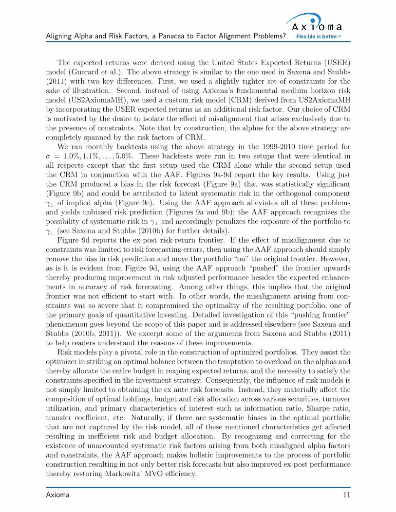
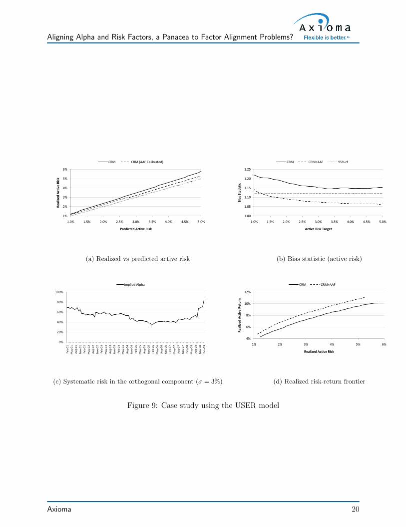
The expected returns were derived using the United States Expected Returns (USER)model (Guerard et al.). The above strategy is similar to the one used in Saxena and Stubbs(2011) with two key differences. First, we used a slightly tighter set of constraints for thesake of illustration. Second, instead of using Axioma’s fundamental medium horizon riskmodel (US2AxiomaMH), we used a custom risk model (CRM) derived from US2AxiomaMHby incorporating the USER expected returns as an additional risk factor. Our choice of CRMis motivated by the desire to isolate the effect of misalignment that arises exclusively due tothe presence of constraints. Note that by construction, the alphas for the above strategy arecompletely spanned by the risk factors of CRM.

We ran monthly backtests using the above strategy in the 1999-2010 time period forσ = 1.0%, 1.1%, . . . , 5.0%. These backtests were run in two setups that were identical inall respects except that the first setup used the CRM alone while the second setup usedthe CRM in conjunction with the AAF. Figures 9a-9d report the key results. Using justthe CRM produced a bias in the risk forecast (Figure 9a) that was statistically significant(Figure 9b) and could be attributed to latent systematic risk in the orthogonal componentγ⊥ of implied alpha (Figure 9c). Using the AAF approach alleviates all of these problemsand yields unbiased risk prediction (Figures 9a and 9b); the AAF approach recognizes thepossibility of systematic risk in γ⊥ and accordingly penalizes the exposure of the portfolio toγ⊥ (see Saxena and Stubbs (2010b) for further details).

Figure 9d reports the ex-post risk-return frontier. If the effect of misalignment due toconstraints was limited to risk forecasting errors, then using the AAF approach should simplyremove the bias in risk prediction and move the portfolio “on” the original frontier. However,as is it is evident from Figure 9d, using the AAF approach “pushed” the frontier upwardsthereby producing improvement in risk adjusted performance besides the expected enhance-ments in accuracy of risk forecasting. Among other things, this implies that the originalfrontier was not efficient to start with. In other words, the misalignment arising from con-straints was so severe that it compromised the optimality of the resulting portfolio, one ofthe primary goals of quantitative investing. Detailed investigation of this “pushing frontier”phenomenon goes beyond the scope of this paper and is addressed elsewhere (see Saxena andStubbs (2010b, 2011)). We excerpt some of the arguments from Saxena and Stubbs (2011)to help readers understand the reasons of these improvements.

Risk models play a pivotal role in the construction of optimized portfolios. They assist theoptimizer in striking an optimal balance between the temptation to overload on the alphas andthereby allocate the entire budget in reaping expected returns, and the necessity to satisfy theconstraints specified in the investment strategy. Consequently, the influence of risk models isnot simply limited to obtaining the ex ante risk forecasts. Instead, they materially affect thecomposition of optimal holdings, budget and risk allocation across various securities, turnoverutilization, and primary characteristics of interest such as information ratio, Sharpe ratio,transfer coefficient, etc. Naturally, if there are systematic biases in the optimal portfoliothat are not captured by the risk model, all of these mentioned characteristics get affectedresulting in inefficient risk and budget allocation. By recognizing and correcting for theexistence of unaccounted systematic risk factors arising from both misaligned alpha factorsand constraints, the AAF approach makes holistic improvements to the process of portfolioconstruction resulting in not only better risk forecasts but also improved ex-post performancethereby restoring Markowitz’ MVO efficiency.

Axioma 11

DRAFT


5 Conclusion

In this paper we set out to illustrate the role of constraints in introducing FAP despitecomplete conformity between alpha and risk factors. We presented several empirical andtheoretical results to corroborate our point of view and in the process of doing so, producedresearch that helps to better understand the mechanics of quantitative portfolio construction.We close the paper with two concluding remarks.

First, even though the impact of constraints is difficult to comprehend, their role shouldnot be under-emphasized or relegated to ancillary status during investigation of quantitativestrategies. The key to understanding the influence of constraints lies in designing experimentsthat can isolate their effects and lend themselves to insightful analysis. The experimentsdiscussed in Section 2 were motivated by these considerations. We encourage the readers toreplicate these experiments and convince themselves that aligning alpha and risk factors isonly a partial remedy to FAP. Second, we want to remind the readers that the alternativesource of misalignment, namely misaligned alpha factors, is equally important and it is thecombination of alpha and constraints that cause FAP. Fortunately, development of productssuch as the Risk Model Machine (RMM), have made it considerably easier to handle FAP dueto misaligned alpha factors. Research efforts to leverage tools such as the RMM in handlingmisalignment arising due to constraints hold clues for further improvements.

Acknowledgement

The first author would like to thank John Guerard for providing access to the USER model.Thanks are also due to Nicole Beard for her help in editing the paper.

Axioma 12

DRAFT


0.0%

1.0%

2.0%

3.0%

4.0%

0.0% 0.5% 1.0% 1.5% 2.0% 2.5% 3.0% 3.5%

Re

aliz

ed

Act

ive

Ris

k

Predicted Active Risk

US2AxiomaSH

(a) Realized vs predicted active risk

1.0

1.1

1.2

1.3

1.4

0.0% 0.5% 1.0% 1.5% 2.0% 2.5% 3.0% 3.5%

Bia

s St

atis

tic

Active Risk Target

Active Risk 95% cf Total Risk

(b) Bias statistic

0%

20%

40%

60%

80%

100%

120%

140%

160%

Dec

-99

Ap

r-0

0

Au

g-0

0

Dec

-00

Ap

r-0

1

Au

g-0

1

Dec

-01

Ap

r-0

2

Au

g-0

2

Dec

-02

Ap

r-0

3

Au

g-0

3

Dec

-03

Ap

r-0

4

Au

g-0

4

Dec

-04

Ap

r-0

5

Au

g-0

5

Dec

-05

Ap

r-0

6

Au

g-0

6

Dec

-06

Ap

r-0

7

Au

g-0

7

Dec

-07

Ap

r-0

8

Au

g-0

8

Dec

-08

Ap

r-0

9

Au

g-0

9

Dec

-09

Ap

r-1

0

Au

g-1

0

Implied Alpha Median Factor Vol (US2AxiomaSH)

(c) Systematic risk in the orthogonal component (σ = 2%)

0%

20%

40%

60%

80%

100%

0.0% 0.5% 1.0% 1.5% 2.0% 2.5% 3.0% 3.5%

Ave

rage

Tu

rno

ver

Active Risk Target

Average Turnover

(d) Average turnover

Figure 1: Base Strategy Results

Figures

Axioma 13

DRAFT


0%

20%

40%

60%

80%

100%

Jan-98

Jun-98

Nov-98

Apr-99

Sep-99

Feb-00

Jul-00

Dec-00

May-01

Oct-01

Mar-02

Aug-02

Jan-03

Jun-03

Nov-03

Apr-04

Sep-04

Feb-05

Jul-05

Dec-05

May-06

Oct-06

Mar-07

Aug-07

Jan-08

Jun-08

Nov-08

Apr-09

Sep-09

Feb-10

Jul-10

Spanned Orthogonal

(a) Spanned vs Orthogonal Component

0%

20%

40%

60%

80%

Dec

-99

May

-00

Oct

-00

Mar

-01

Au

g-0

1

Jan

-02

Jun

-02

No

v-0

2

Ap

r-0

3

Sep

-03

Feb

-04

Jul-

04

Dec

-04

May

-05

Oct

-05

Mar

-06

Au

g-0

6

Jan

-07

Jun

-07

No

v-0

7

Ap

r-0

8

Sep

-08

Feb

-09

Jul-

09

Dec

-09

May

-10

Oct

-10

Re

aliz

ed

Sys

tem

atic

ris

k in

ort

ho

gon

al

com

po

ne

nt

Tail Alpha

(b) Systematic risk in the orthogonal component

Figure 2: Alignment analysis of tail alpha

0.0%

1.0%

2.0%

3.0%

4.0%

0.0% 0.5% 1.0% 1.5% 2.0% 2.5% 3.0% 3.5%

Re

aliz

ed

Act

ive

Ris

k


US2AxiomaSH


1.0

1.1

1.2

1.3

1.4

0.0% 0.5% 1.0% 1.5% 2.0% 2.5% 3.0% 3.5%

Bia

s St

atis

tic

Active Risk Target

US2AxiomaSH 95% cf

(b) Bias statistic (active risk)

0%

20%

40%

60%

80%

Dec

-99

Ap

r-0

0

Au

g-0

0

Dec

-00

Ap

r-0

1

Au

g-0

1

Dec

-01

Ap

r-0

2

Au

g-0

2

Dec

-02

Ap

r-0

3

Au

g-0

3

Dec

-03

Ap

r-0

4

Au

g-0

4

Dec

-04

Ap

r-0

5

Au

g-0

5

Dec

-05

Ap

r-0

6

Au

g-0

6

Dec

-06

Ap

r-0

7

Au

g-0

7

Dec

-07

Ap

r-0

8

Au

g-0

8

Dec

-08

Ap

r-0

9

Au

g-0

9

Dec

-09

Ap

r-1

0

Au

g-1

0

Implied Alpha


0%

20%

40%

60%

80%

100%

0.00% 0.50% 1.00% 1.50% 2.00% 2.50% 3.00% 3.50%

Ave

rage

Tu

rno

ver

Active Risk Target

Average Turnover


Figure 3: Base Strategy with turnover constraint

Axioma 14

DRAFT


0.0%

1.0%

2.0%

3.0%

4.0%

0.0% 0.5% 1.0% 1.5% 2.0% 2.5% 3.0% 3.5%

Re

aliz

ed

Act

ive

Ris

k


US2AxiomaSH


1.0

1.1

1.2

1.3

1.4

0.0% 0.5% 1.0% 1.5% 2.0% 2.5% 3.0% 3.5%

Bia

s St

atis

tic

Active Risk Target

US2AxiomaSH 95% cf


0%

20%

40%

60%

80%

Dec

-99

Ap

r-0

0

Au

g-0

0

Dec

-00

Ap

r-0

1

Au

g-0

1

Dec

-01

Ap

r-0

2

Au

g-0

2

Dec

-02

Ap

r-0

3

Au

g-0

3

Dec

-03

Ap

r-0

4

Au

g-0

4

Dec

-04

Ap

r-0

5

Au

g-0

5

Dec

-05

Ap

r-0

6

Au

g-0

6

Dec

-06

Ap

r-0

7

Au

g-0

7

Dec

-07

Ap

r-0

8

Au

g-0

8

Dec

-08

Ap

r-0

9

Au

g-0

9

Dec

-09

Ap

r-1

0

Au

g-1

0

Implied Alpha


0%

20%

40%

60%

80%

100%

0.00% 0.50% 1.00% 1.50% 2.00% 2.50% 3.00% 3.50%

Ave

rage

Tu

rno

ver

Active Risk Target

Average Turnover


Figure 4: Base Strategy with transaction cost objective term

Axioma 15

DRAFT


0.0%

1.0%

2.0%

3.0%

4.0%

5.0%

0.0% 0.5% 1.0% 1.5% 2.0% 2.5% 3.0% 3.5%

Re

aliz

ed

Act

ive

Ris

k


US2AxiomaSH


1.0

1.1

1.2

1.3

1.4

0.0% 0.5% 1.0% 1.5% 2.0% 2.5% 3.0% 3.5%

Bia

s St

atis

tic

Active Risk Target

US2AxiomaSH 95% cf


0%

20%

40%

60%

80%

100%

Dec

-99

Ap

r-0

0

Au

g-0

0

Dec

-00

Ap

r-0

1

Au

g-0

1

Dec

-01

Ap

r-0

2

Au

g-0

2

Dec

-02

Ap

r-0

3

Au

g-0

3

Dec

-03

Ap

r-0

4

Au

g-0

4

Dec

-04

Ap

r-0

5

Au

g-0

5

Dec

-05

Ap

r-0

6

Au

g-0

6

Dec

-06

Ap

r-0

7

Au

g-0

7

Dec

-07

Ap

r-0

8

Au

g-0

8

Dec

-08

Ap

r-0

9

Au

g-0

9

Dec

-09

Ap

r-1

0

Au

g-1

0

Implied Alpha


0%

20%

40%

60%

80%

100%

0.00% 0.50% 1.00% 1.50% 2.00% 2.50% 3.00% 3.50%

Ave

rage

Tu

rno

ver

Active Risk Target

Average Turnover


Figure 5: Base Strategy with market impact function objective term

Axioma 16

DRAFT


0.0%

1.0%

2.0%

3.0%

4.0%

0.0% 0.5% 1.0% 1.5% 2.0% 2.5% 3.0% 3.5%

Re

aliz

ed

Act

ive

Ris

k


US2AxiomaSH


1.0

1.1

1.2

1.3

1.4

0.0% 0.5% 1.0% 1.5% 2.0% 2.5% 3.0% 3.5%

Bia

s St

atis

tic

Active Risk Target

US2AxiomaSH 95% cf


0%

40%

80%

120%

Dec

-99

May

-00

Oct

-00

Mar

-01

Au

g-0

1

Jan

-02

Jun

-02

No

v-0

2

Ap

r-0

3

Sep

-03

Feb

-04

Jul-

04

Dec

-04

May

-05

Oct

-05

Mar

-06

Au

g-0

6

Jan

-07

Jun

-07

No

v-0

7

Ap

r-0

8

Sep

-08

Feb

-09

Jul-

09

Dec

-09

May

-10

Oct

-10

Implied Alpha


0%

20%

40%

60%

80%

100%

0.00% 0.50% 1.00% 1.50% 2.00% 2.50% 3.00% 3.50%

Ave

rage

Tu

rno

ver

Active Risk Target

Average Turnover


Figure 6: Base Strategy with Average Daily Volume (ADV) constraint

Axioma 17

DRAFT


0.0%

1.0%

2.0%

3.0%

4.0%

5.0%

0.0% 0.5% 1.0% 1.5% 2.0% 2.5% 3.0% 3.5%

Re

aliz

ed

Act

ive

Ris

k


US2AxiomaSH


1.0

1.1

1.2

1.3

1.4

0.0% 0.5% 1.0% 1.5% 2.0% 2.5% 3.0% 3.5%

Bia

s St

atis

tic

Active Risk Target

US2AxiomaSH 95% cf


0%

20%

40%

60%

80%

100%

Dec

-99

Ap

r-0

0

Au

g-0

0

Dec

-00

Ap

r-0

1

Au

g-0

1

Dec

-01

Ap

r-0

2

Au

g-0

2

Dec

-02

Ap

r-0

3

Au

g-0

3

Dec

-03

Ap

r-0

4

Au

g-0

4

Dec

-04

Ap

r-0

5

Au

g-0

5

Dec

-05

Ap

r-0

6

Au

g-0

6

Dec

-06

Ap

r-0

7

Au

g-0

7

Dec

-07

Ap

r-0

8

Au

g-0

8

Dec

-08

Ap

r-0

9

Au

g-0

9

Dec

-09

Ap

r-1

0

Au

g-1

0

Implied Alpha


0%

20%

40%

60%

80%

100%

0.0% 0.5% 1.0% 1.5% 2.0% 2.5% 3.0% 3.5%

Ave

rage

Tu

rno

ver

Active Risk Target

Average Turnover


Figure 7: Base Strategy with illiquidity motivated active asset bounds

Axioma 18

DRAFT


0.0%

1.0%

2.0%

3.0%

4.0%

5.0%

6.0%

0 0.005 0.01 0.015 0.02 0.025 0.03 0.035

Re

aliz

ed

Act

ive

Ris

k


US2AxiomaMH


1.0

1.1

1.2

1.3

1.4

0.0% 0.5% 1.0% 1.5% 2.0% 2.5% 3.0% 3.5%

Bia

s St

atis

tic

Active Risk Target

US2AxiomaMH 95% cf


0%

20%

40%

60%

Dec

-98

Ap

r-9

9

Au

g-9

9

Dec

-99

Ap

r-0

0

Au

g-0

0

Dec

-00

Ap

r-0

1

Au

g-0

1

Dec

-01

Ap

r-0

2

Au

g-0

2

Dec

-02

Ap

r-0

3

Au

g-0

3

Dec

-03

Ap

r-0

4

Au

g-0

4

Dec

-04

Ap

r-0

5

Au

g-0

5

Dec

-05

Ap

r-0

6

Au

g-0

6

Dec

-06

Ap

r-0

7

Au

g-0

7

Dec

-07

Ap

r-0

8

Au

g-0

8

Dec

-08

Ap

r-0

9

Au

g-0

9

Implied Alpha


0%

20%

40%

60%

80%

100%

0.00% 0.50% 1.00% 1.50% 2.00% 2.50% 3.00% 3.50%

Ave

rage

Tu

rno

ver

Active Risk Target

Average Turnover


Figure 8: Variant of the base strategy that uses large-cap asset universe and medium-horizonfundamental risk model

Axioma 19

DRAFT


1%

2%

3%

4%

5%

6%

1.0% 1.5% 2.0% 2.5% 3.0% 3.5% 4.0% 4.5% 5.0%

Re

aliz

ed

Act

ive

Ris

k


CRM CRM (AAF Calibrated)


1.00

1.05

1.10

1.15

1.20

1.25

1.0% 1.5% 2.0% 2.5% 3.0% 3.5% 4.0% 4.5% 5.0%

Bia

s St

atis

tic

Active Risk Target

CRM CRM+AAF 95% cf


0%

20%

40%

60%

80%

100%

Feb

-01

May

-01

Au

g-0

1

No

v-0

1

Feb

-02

May

-02

Au

g-0

2

No

v-0

2

Feb

-03

May

-03

Au

g-0

3

No

v-0

3

Feb

-04

May

-04

Au

g-0

4

No

v-0

4

Feb

-05

May

-05

Au

g-0

5

No

v-0

5

Feb

-06

May

-06

Au

g-0

6

No

v-0

6

Feb

-07

May

-07

Au

g-0

7

No

v-0

7

Feb

-08

May

-08

Au

g-0

8

No

v-0

8

Feb

-09

Implied Alpha


4%

6%

8%

10%

12%

1% 2% 3% 4% 5% 6%

Re

aliz

ed

Act

ive

Re

turn

Realized Active Risk

CRM CRM+AAF

(d) Realized risk-return frontier

Figure 9: Case study using the USER model

Axioma 20

DRAFT


References

A. Alford, R. Jones, and Lim T. Equity portfolio management. In Modern InvestmentManagement: An Equilibrium Approach, chapter 23, pages 416–434. John Wiley & Sons,Inc., Hoboken, New Jersey, 2003.

S. Ceria, A. Saxena, and R. A. Stubbs. Factor alignment problems and quantitative portfoliomanagement. Journal of Portfolio Management, To Appear, 2012.

J.B. Jr. Guerard, M.N. Gultekin, , and G. Xu. Investing with momentum: The past, present,and future. Journal of Investing, To Appear.

Jyh-Huei Lee and Dan Stefek. Do risk factors eat alphas? The Journal of Portfolio Man-agement, 34(4):12–25, Summer 2008.

A. A. Renshaw, R. A. Stubbs, S. Schmieta, and S. Ceria. Axioma alpha factor method:Improving risk estimation by reducing risk model portfolio selection bias. Technical report,Axioma, Inc. Research Report, March 2006.

A. Saxena and R. A. Stubbs. Alpha alignment factor: A solution to the underestimation ofrisk for optimized active portfolios. Technical report, Axioma, Inc. Research Report #015,February 2010a.

A. Saxena and R. A. Stubbs. Pushing frontiers (literally) using alpha alignment factor.Technical report, Axioma, Inc. Research Report #022, February 2010b.

A. Saxena and R. A. Stubbs. An empirical case study of factor alignment problems usingthe united states expected returns (user) model. Technical report, Axioma, Inc. ResearchReport #036, October 2011.

Axioma 21

United States and Canada: 212-991-4500

Europe: +44 20 7856 2451

Asia: +852-8203-2790

New York OfficeAxioma, Inc.17 State StreetSuite 2550New York, NY 10004

Phone: 212-991-4500Fax: 212-991-4539

London OfficeAxioma, (UK) Ltd.30 Crown PlaceLondon, EC2A 4EB

Phone: +44 (0) 20 7856 2451Fax: +44 (0) 20 3006 8747

Atlanta OfficeAxioma, Inc.8800 Roswell RoadBuilding B, Suite 295Atlanta, GA 30350

Phone: 678-672-5400Fax: 678-672-5401

Hong Kong OfficeAxioma, (HK) Ltd.Unit B, 17/F, Entertainment Building30 Queen’s Road CentralHong Kong

Phone: +852-8203-2790Fax: +852-8203-2774

San Francisco OfficeAxioma, Inc.201 Mission StreetSuite #2230San Francisco, CA 94105

Phone: 415-614-4170Fax: 415-614-4169

Singapore OfficeAxioma, (Asia) Pte Ltd.30 Raffles Place#23-00 Chevron HouseSingapore 048622

Phone: +65 6233 6835Fax: +65 6233 6891

Geneva OfficeAxioma CHRue du Rhone 69, 2nd Floor1207 Geneva, Switzerland

Phone: +33 611 96 81 53

Sydney OfficeAxioma AULevel 4,5 & 1295 Pitt Street, 506bNSW 2000Sydney, Australia

Phone: +61 (2) 8079 2915

Sales: [email protected]

Client Support: [email protected]

Careers: [email protected]

DRAFT

Documents

DRAFT - Axioma | Home Pages/alighningalpha...DRAFT Aligning Alpha and Risk Factors, a Panacea to Factor Alignment Problems? implied alpha,?, can still be non-zero, have overlap with