Dr. Sameer Mulani

Co-PI

Two papers:

Wing-Box Weight Optimization Using Curvilinear Spars and Ribs

(SpaRibs)

Nonstationary Random Vibration Analysis of Wing with Geometric

Nonlinearity Under Correlated Excitation

Wing-Box Weight Optimization Using Curvilinear Sparsand Ribs (SpaRibs)

Davide Locatelli,∗ Sameer B. Mulani,† and Rakesh K. Kapania‡

Virginia Polytechnic Institute and State University, Blacksburg, Virginia 24061-0203

DOI: 10.2514/1.C031336

The aim of this research is to perform topology and sizing optimization of wing-box structures using curvilinear

spars and ribs, referred to as SpaRibs in the following. To accomplish this, a new framework calledEBF3SSWingOpt

is being developed at Virginia Polytechnic Institute and State University. The optimization framework includes two

different methodologies: a one-step optimization methodology where topology and sizing optimization are carried

out together and a two-step optimization methodology where topology and sizing optimization are carried out

separately using different constraints and objective functions. A description of how the general framework is

developed and applied for optimizing winglike structures is provided and the optimization-problem formulation is

stated. Two practical design problems solved using EBF3SSWingOpt are presented: a rectangular wing box and a

generic fighter wing. In both cases, the structure with the SpaRibs is lighter than the initial structure with straight

spars and ribs.Moreover, the two-step optimization framework has proven to be better atfinding anoptimal solution

than the one-step framework. Finally, different designs with comparable weights but different stress distributions,

buckling properties, and dynamic behaviors were found.

Nomenclature

Ai = ith finite element areaBF0 = buckling factorEBF3 = electron beam free-form fabricationf�x� = optimization objective functiongi�x� = ith optimization constraint functionKSC� = Kreisselmeier–Steinhauser stress coefficientniter = number of iterationsP = applied loadPcr = critical buckling loadSF = safety factorTCPU = CPU timeW = weightWMAX = maximum weightx = design-variable vectorxjMAX = jth design-variable upper boundaryxjmin = jth design-variable lower boundary�0 = fundamental buckling eigenvalue� = Kreisselmeier–Steinhauser constant�i = ith finite element von Mises stress�u = ultimate tension stress�VM = von Mises stress�y = yield stress of the material

I. Introduction

T HE present work is motivated by the fact that to enhancestructural performance in aerospace field, new design concepts

for aircraft structures are needed. Two aspects are of particular

interest for industry and manufacturing: bring design optimizationand high-fidelity analysis in the early stages of design and bringtogether asmanydisciplines as possible. The quest for the best designis dictated by many constraints related to environmental issues,manufacturing time and cost, maintenance cost, and operational cost,which have to be added to the typical structural integrity and safetyconstraints. As a consequence, nowadays, engineers are challengedto take into account all these aspects during the early stages ofconcept design, and they need new analysis tools to accomplish thiscomplex task.

The biggest limitation in classic structural design is the use of verysimple components as straight spars and ribs, quadrilateral panels,uniform-thickness stiffeners, and stringers. Moreover, all thesestructural elements have to be connected using bolts and rivets or bywelding,which are time- andmoney-consuming processes. Thus, thetrend in the industry is toward designing structures with fewercomponents, but more efficiently. This philosophy leads to thedevelopment of the so-called unitized structures, characterized bythe integration of the stiffening members to the rest of the structureachieving a monolithic construction of the vehicle [1]. Theadvantages of the use of unitized structure [2] over classical designedstructures are multiple and can be identified as follows: 1) reducedpart count, manufacturing time, and fabrication cost; 2) increaseddesign flexibility; 3) weight savings; 4) increased resistance tofatigue and corrosion; 5) enhanced automation; and 6) improvedergonomics and reduced work.

The benefits of unitized structures are so overpowering thatexperts expect an exponential increase in the use of this kind ofstructure in the aeronautics and aerospace design by 2020 [1]. Majoraircraft manufacturer companies lead this revolution in structuraldesign approach. In particular, Boeing already has developed a newintegrally stiffened fuselage concept whose testing demonstratedstructural performance and efficiency similar to those of conven-tional design, while achieving significant manufacturing time andcost reduction [3]. The manufacturing of unitized structures isdirectly linked to the development of new innovative manufacturingtechniques as rapid manufacturing, rapid prototyping, solid free-form fabrication, and additive manufacturing [4,5]. Friction stirwelding [6] and electron beam free-form fabrication (EBF3) [7–9]are among the most promising manufacturing techniques that can beused to produce metallic unitized structures for the aeronauticsindustry. Furthermore, these techniques enable the manufacturing ofintegrated curvilinear stiffening members with negligible additionalcost and time with respect to conventional processes. This aspect iscrucial for the optimization of the airframe components, since

Presented at the 51st AIAA/ASME/ASCE/AHS/ASC Structures,Structural Dynamics and Material Conference, Orlando, FL, 10–15 April2010; received 8 December 2010; revision received 18 April 2011; acceptedfor publication 19April 2011. Copyright©2011 byDavideLocatelli, SameerB. Mulani, and Rakesh K. Kapania. Published by the American Institute ofAeronautics andAstronautics, Inc., with permission. Copies of this papermaybe made for personal or internal use, on condition that the copier pay the$10.00 per-copy fee to the Copyright Clearance Center, Inc., 222 RosewoodDrive, Danvers, MA 01923; include the code 0021-8669/11 and $10.00 incorrespondence with the CCC.

∗Research Assistant, Engineering Science and Mechanics. StudentMember AIAA.

†Postdoctoral Fellow, Aerospace and Ocean Engineering. Senior MemberAIAA.

‡Mitchell Professor, Aerospace and Ocean Engineering. Associate FellowAIAA.

JOURNAL OF AIRCRAFT

Vol. 48, No. 5, September–October 2011

1671

Dow

nloa

ded

by U

NIV

ER

SIT

Y O

F A

LA

BA

MA

on

Oct

ober

2, 2

018

| http

://ar

c.ai

aa.o

rg |

DO

I: 1

0.25

14/1

.C03

1336

topology optimization methods lead often to curved designs [10].The use of curved stiffening members broadens the design space andprovides variable stiffness, enabling a more efficient structural andmaterial tailoring. The concept of variable stiffness is not new inaeronautical design. In fact, nonuniformly stiffened structures havebeen used in the construction of airframes since the dawn of aero-space history. Straight stiffeners are commonly used to providepanels with additional stiffness along the direction of the acting loads[11]. Moreover, the stiffeners can be placed at different orientationsto alignwith the stress flow in the structure and to provide an efficientload-bearing mechanism. Use of multiple stiffeners is also advan-tageous, since it provides redundancy and efficiently stops thegrowth of cracks in the supporting substructure [11]. A further im-provement in airframe panel design is represented by the introductionof geodesically stiffened panels, whose optimization and structuralresponse was widely studied by Gürdal and Gendron [12], Gürdaland Grall [13], Gendron and Gürdal [14], and Grall and Gürdal [15].Isogrid [16] and grid-stiffened [17,18] panels are also commonlyused in aircraft design for their efficiency in load-carrying capabilityand buckling behavior [19].

The broad use of compositematerials is alsomotivated by the needfor nonuniformly stiffened structures. Hence, the composites havealways been an integral part of aircraft structural layout, from thewood ply composite materials introduced in the 1920s [20] to themost advanced nonuniformly distributed curved fibers and matrixcomposites used for differential stiffening of fuselage structures [21].

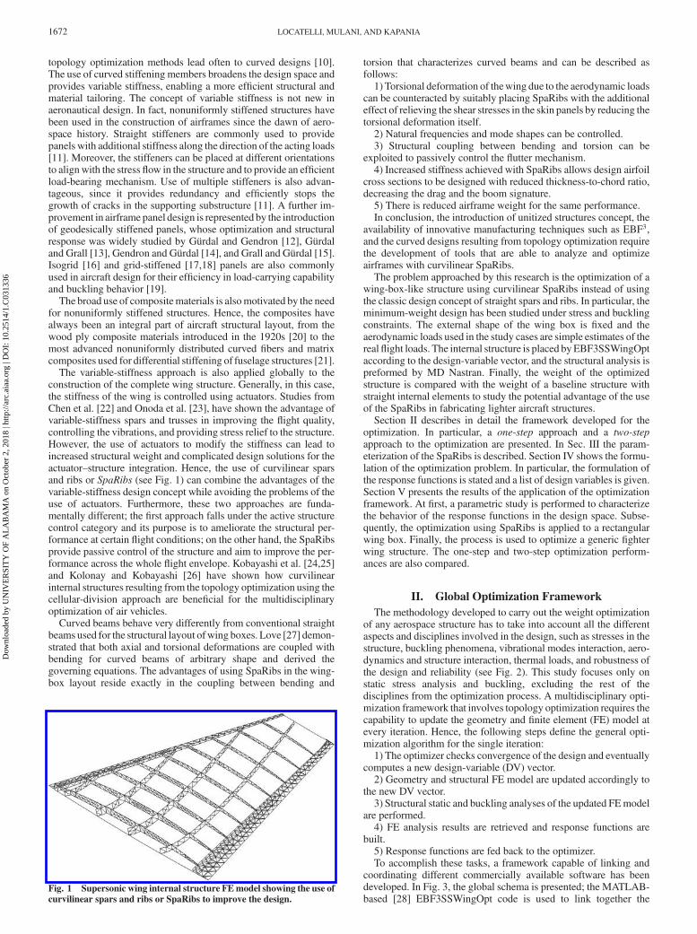
The variable-stiffness approach is also applied globally to theconstruction of the complete wing structure. Generally, in this case,the stiffness of the wing is controlled using actuators. Studies fromChen et al. [22] and Onoda et al. [23], have shown the advantage ofvariable-stiffness spars and trusses in improving the flight quality,controlling the vibrations, and providing stress relief to the structure.However, the use of actuators to modify the stiffness can lead toincreased structural weight and complicated design solutions for theactuator–structure integration. Hence, the use of curvilinear sparsand ribs or SpaRibs (see Fig. 1) can combine the advantages of thevariable-stiffness design concept while avoiding the problems of theuse of actuators. Furthermore, these two approaches are funda-mentally different; the first approach falls under the active structurecontrol category and its purpose is to ameliorate the structural per-formance at certain flight conditions; on the other hand, the SpaRibsprovide passive control of the structure and aim to improve the per-formance across the whole flight envelope. Kobayashi et al. [24,25]and Kolonay and Kobayashi [26] have shown how curvilinearinternal structures resulting from the topology optimization using thecellular-division approach are beneficial for the multidisciplinaryoptimization of air vehicles.

Curved beams behave very differently from conventional straightbeams used for the structural layout ofwing boxes. Love [27] demon-strated that both axial and torsional deformations are coupled withbending for curved beams of arbitrary shape and derived thegoverning equations. The advantages of using SpaRibs in the wing-box layout reside exactly in the coupling between bending and

torsion that characterizes curved beams and can be described asfollows:

1) Torsional deformation of thewing due to the aerodynamic loadscan be counteracted by suitably placing SpaRibs with the additionaleffect of relieving the shear stresses in the skin panels by reducing thetorsional deformation itself.

2) Natural frequencies and mode shapes can be controlled.3) Structural coupling between bending and torsion can be

exploited to passively control the flutter mechanism.4) Increased stiffness achieved with SpaRibs allows design airfoil

cross sections to be designed with reduced thickness-to-chord ratio,decreasing the drag and the boom signature.

5) There is reduced airframe weight for the same performance.In conclusion, the introduction of unitized structures concept, the

availability of innovative manufacturing techniques such as EBF3,and the curved designs resulting from topology optimization requirethe development of tools that are able to analyze and optimizeairframes with curvilinear SpaRibs.

The problem approached by this research is the optimization of awing-box-like structure using curvilinear SpaRibs instead of usingthe classic design concept of straight spars and ribs. In particular, theminimum-weight design has been studied under stress and bucklingconstraints. The external shape of the wing box is fixed and theaerodynamic loads used in the study cases are simple estimates of therealflight loads. The internal structure is placed byEBF3SSWingOptaccording to the design-variable vector, and the structural analysis ispreformed by MD Nastran. Finally, the weight of the optimizedstructure is compared with the weight of a baseline structure withstraight internal elements to study the potential advantage of the useof the SpaRibs in fabricating lighter aircraft structures.

Section II describes in detail the framework developed for theoptimization. In particular, a one-step approach and a two-stepapproach to the optimization are presented. In Sec. III the param-eterization of the SpaRibs is described. Section IV shows the formu-lation of the optimization problem. In particular, the formulation ofthe response functions is stated and a list of design variables is given.Section V presents the results of the application of the optimizationframework. At first, a parametric study is performed to characterizethe behavior of the response functions in the design space. Subse-quently, the optimization using SpaRibs is applied to a rectangularwing box. Finally, the process is used to optimize a generic fighterwing structure. The one-step and two-step optimization perform-ances are also compared.

II. Global Optimization Framework

The methodology developed to carry out the weight optimizationof any aerospace structure has to take into account all the differentaspects and disciplines involved in the design, such as stresses in thestructure, buckling phenomena, vibrational modes interaction, aero-dynamics and structure interaction, thermal loads, and robustness ofthe design and reliability (see Fig. 2). This study focuses only onstatic stress analysis and buckling, excluding the rest of thedisciplines from the optimization process. A multidisciplinary opti-mization framework that involves topology optimization requires thecapability to update the geometry and finite element (FE) model atevery iteration. Hence, the following steps define the general opti-mization algorithm for the single iteration:

1) The optimizer checks convergence of the design and eventuallycomputes a new design-variable (DV) vector.

2) Geometry and structural FE model are updated accordingly tothe new DV vector.

3) Structural static and buckling analyses of the updated FEmodelare performed.

4) FE analysis results are retrieved and response functions arebuilt.

5) Response functions are fed back to the optimizer.To accomplish these tasks, a framework capable of linking and

coordinating different commercially available software has beendeveloped. In Fig. 3, the global schema is presented; the MATLAB-based [28] EBF3SSWingOpt code is used to link together the

Fig. 1 Supersonic wing internal structure FEmodel showing the use of

curvilinear spars and ribs or SpaRibs to improve the design.

1672 LOCATELLI, MULANI, AND KAPANIA

Dow

nloa

ded

by U

NIV

ER

SIT

Y O

F A

LA

BA

MA

on

Oct

ober

2, 2

018

| http

://ar

c.ai

aa.o

rg |

DO

I: 1

0.25

14/1

.C03

1336

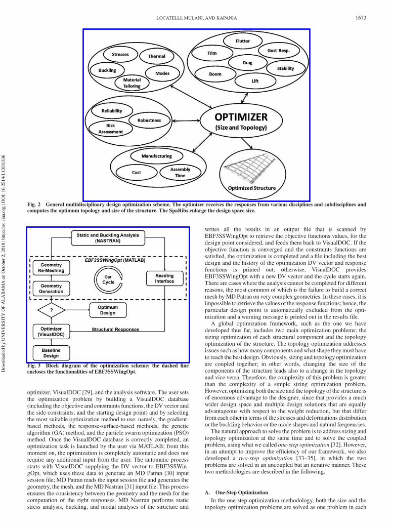
optimizer, VisualDOC [29], and the analysis software. The user setsthe optimization problem by building a VisualDOC database(including the objective and constraints functions, the DV vector andthe side constraints, and the starting design point) and by selectingthe most suitable optimization method to use: namely, the gradient-based methods, the response-surface-based methods, the geneticalgorithm (GA) method, and the particle swarm optimization (PSO)method. Once the VisualDOC database is correctly completed, anoptimization task is launched by the user via MATLAB; from thismoment on, the optimization is completely automatic and does notrequire any additional input from the user. The automatic processstarts with VisualDOC supplying the DV vector to EBF3SSWin-gOpt, which uses these data to generate an MD Patran [30] inputsession file; MD Patran reads the input session file and generates thegeometry, the mesh, and theMDNastran [31] input file. This processensures the consistency between the geometry and the mesh for thecomputation of the right responses. MD Nastran performs staticstress analysis, buckling, and modal analyses of the structure and

writes all the results in an output file that is scanned byEBF3SSWingOpt to retrieve the objective functions values, for thedesign point considered, and feeds them back to VisualDOC. If theobjective function is converged and the constraints functions aresatisfied, the optimization is completed and a file including the bestdesign and the history of the optimization DV vector and responsefunctions is printed out; otherwise, VisualDOC providesEBF3SSWingOpt with a new DV vector and the cycle starts again.There are cases where the analysis cannot be completed for differentreasons, the most common of which is the failure to build a correctmesh byMD Patran on very complex geometries. In these cases, it isimpossible to retrieve the values of the response functions; hence, theparticular design point is automatically excluded from the opti-mization and a warning message is printed out in the results file.

A global optimization framework, such as the one we havedeveloped thus far, includes two main optimization problems; thesizing optimization of each structural component and the topologyoptimization of the structure. The topology optimization addressesissues such as howmany components andwhat shape theymust haveto reach the best design. Obviously, sizing and topology optimizationare coupled together; in other words, changing the size of thecomponents of the structure leads also to a change in the topologyand vice versa. Therefore, the complexity of this problem is greaterthan the complexity of a simple sizing optimization problem.However, optimizing both the size and the topology of the structure isof enormous advantage to the designer, since that provides a muchwider design space and multiple design solutions that are equallyadvantageous with respect to the weight reduction, but that differfrom each other in terms of the stresses and deformations distributionor the buckling behavior or the mode shapes and natural frequencies.

The natural approach to solve the problem is to address sizing andtopology optimization at the same time and to solve the coupledproblem, using what we called one-step optimization [32]. However,in an attempt to improve the efficiency of our framework, we alsodeveloped a two-step optimization [33–35], in which the twoproblems are solved in an uncoupled but an iterative manner. Thesetwo methodologies are described in the following.

A. One-Step Optimization

In the one-step optimization methodology, both the size and thetopology optimization problems are solved as one problem in each

Fig. 2 General multidisciplinary design optimization scheme. The optimizer receives the responses from various disciplines and subdisciplines and

computes the optimum topology and size of the structure. The SpaRibs enlarge the design space size.

Fig. 3 Block diagram of the optimization scheme; the dashed line

encloses the functionalities of EBF3SSWingOpt.

LOCATELLI, MULANI, AND KAPANIA 1673

Dow

nloa

ded

by U

NIV

ER

SIT

Y O

F A

LA

BA

MA

on

Oct

ober

2, 2

018

| http

://ar

c.ai

aa.o

rg |

DO

I: 1

0.25

14/1

.C03

1336

iteration according to the general scheme presented in Fig. 3. Theweight of the structure isminimized subject to the stress and bucklingconstraints, as shown in Table 1. Performing an optimization usingthis method can require extensive CPU time, due to the large numberof design variables; however, it has the advantage that the user has tobuild just one VisualDOC database and there is no need to iteratebetween sizing and shape optimization to achieve the convergence ofthe objective function.

B. Two-Step Optimization

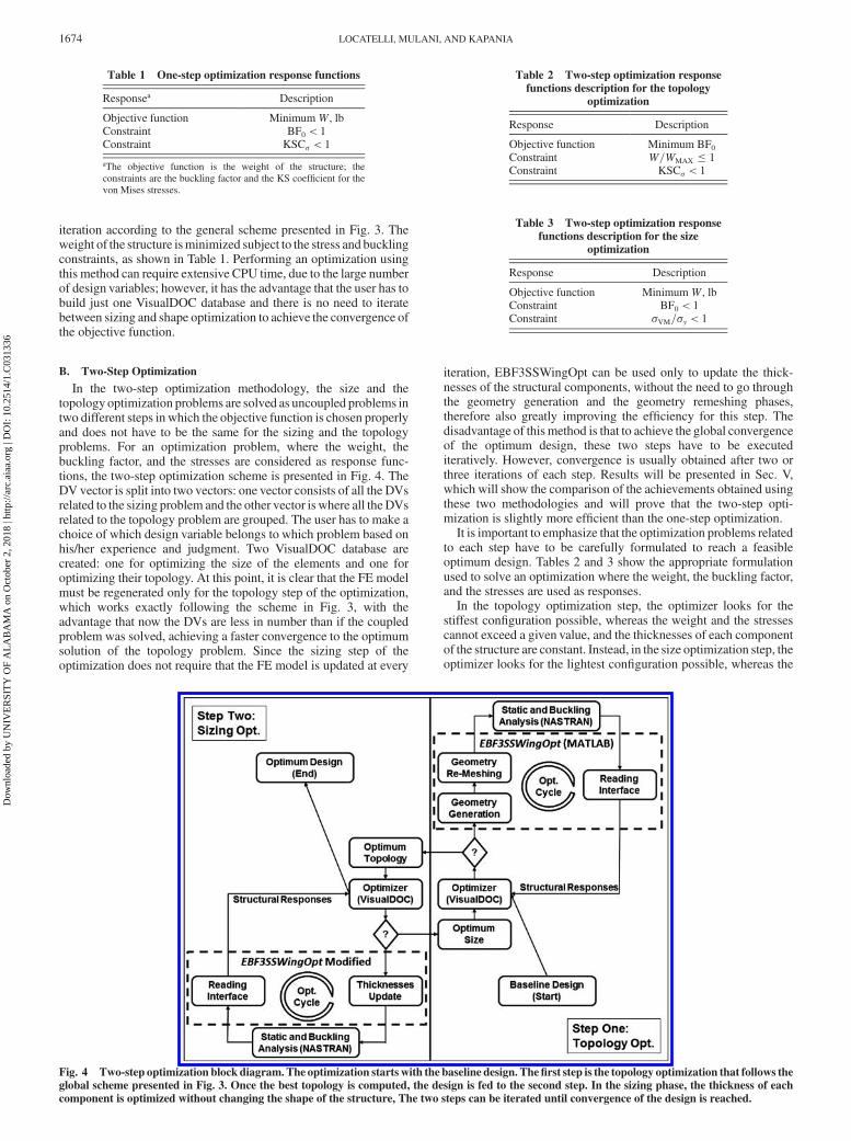
In the two-step optimization methodology, the size and thetopology optimization problems are solved as uncoupled problems intwo different steps in which the objective function is chosen properlyand does not have to be the same for the sizing and the topologyproblems. For an optimization problem, where the weight, thebuckling factor, and the stresses are considered as response func-tions, the two-step optimization scheme is presented in Fig. 4. TheDV vector is split into two vectors: one vector consists of all the DVsrelated to the sizing problem and the other vector is where all theDVsrelated to the topology problem are grouped. The user has to make achoice of which design variable belongs to which problem based onhis/her experience and judgment. Two VisualDOC database arecreated: one for optimizing the size of the elements and one foroptimizing their topology. At this point, it is clear that the FE modelmust be regenerated only for the topology step of the optimization,which works exactly following the scheme in Fig. 3, with theadvantage that now the DVs are less in number than if the coupledproblem was solved, achieving a faster convergence to the optimumsolution of the topology problem. Since the sizing step of theoptimization does not require that the FE model is updated at every

iteration, EBF3SSWingOpt can be used only to update the thick-nesses of the structural components, without the need to go throughthe geometry generation and the geometry remeshing phases,therefore also greatly improving the efficiency for this step. Thedisadvantage of this method is that to achieve the global convergenceof the optimum design, these two steps have to be executediteratively. However, convergence is usually obtained after two orthree iterations of each step. Results will be presented in Sec. V,which will show the comparison of the achievements obtained usingthese two methodologies and will prove that the two-step opti-mization is slightly more efficient than the one-step optimization.

It is important to emphasize that the optimization problems relatedto each step have to be carefully formulated to reach a feasibleoptimum design. Tables 2 and 3 show the appropriate formulationused to solve an optimization where the weight, the buckling factor,and the stresses are used as responses.

In the topology optimization step, the optimizer looks for thestiffest configuration possible, whereas the weight and the stressescannot exceed a given value, and the thicknesses of each componentof the structure are constant. Instead, in the size optimization step, theoptimizer looks for the lightest configuration possible, whereas the

Fig. 4 Two-step optimization block diagram.The optimization starts with the baseline design. The first step is the topology optimization that follows the

global scheme presented in Fig. 3. Once the best topology is computed, the design is fed to the second step. In the sizing phase, the thickness of each

component is optimized without changing the shape of the structure, The two steps can be iterated until convergence of the design is reached.

Table 1 One-step optimization response functions

Responsea Description

Objective function MinimumW, lbConstraint BF0 < 1Constraint KSC� < 1

aThe objective function is the weight of the structure; theconstraints are the buckling factor and the KS coefficient for thevon Mises stresses.

Table 2 Two-step optimization response

functions description for the topology

optimization

Response Description

Objective function Minimum BF0

Constraint W=WMAX � 1Constraint KSC� < 1

Table 3 Two-step optimization response

functions description for the sizeoptimization

Response Description

Objective function MinimumW, lbConstraint BF0 < 1Constraint �VM=�y < 1

1674 LOCATELLI, MULANI, AND KAPANIA

Dow

nloa

ded

by U

NIV

ER

SIT

Y O

F A

LA

BA

MA

on

Oct

ober

2, 2

018

| http

://ar

c.ai

aa.o

rg |

DO

I: 1

0.25

14/1

.C03

1336

buckling factor has to be smaller than 1, the von Mises stresses islower than the yield stress of the material, and the topology of thestructure is fixed.

III. Wing Parametric Geometry Generation

In Sec. II, the general optimization approach was presented. It isimportant to understand that the global schema is applicable to anytype of structure and, in principle, could include any type of responsefunctions and constraints provided by specific disciplines related tothe design. In the following section, the application of the globalschema to the design of winglike structures is described. Thepeculiarity of these kinds of structures is the use of three types ofcomponents that are different for their design and load-carryingfunctions. The components are the skin panels, the spars, and the ribs.To carry out an optimization process that involves topology opti-mization, a geometry parameterization of the structural componentsis needed. The parameters chosen to describe the geometry of thestructural elements will be used as topology-related DVs.

There are multiple equivalent ways to parameterize the geometryof the structure according to different user requirements. In this case,the wing planform and the airfoil cross section are fixed during theoptimization, whereas the shape of spars and ribs is changing; hence,

for our purposes, only the parameterization of the internal structuralcomponents was needed. Our choicewas mainly dictated by how thegeometry is generated inMDPatran; as a consequence, it was naturalto choose the B-spline utility of MD Patran to parametrize the shapeof the SpaRibs. Figure 5 shows how the SpaRibs are generated usingB-splines and the concepts of base curves and bounding box [36].

Base curves are generated interpolating three points, indicated inFig. 5, as the start point, the control point, and the endpoint, withMDPatran B-spline utility. The start- and endpoints of each base curveare always located on two opposite edges of the bounding box, arectangle whose dimensions are constant and provided by the user,enclosing the projection of thewing planform on theX–Y plane. TheSpaRibs are then generated translating each of the base curves in Xand Y directions, respectively, as displayed in Fig. 6.

This formulation allows the reduction from six to four parametersto describe each base curve. To generate a B-spline curve, the usershould provide the coordinates of the start, the control, and theendpoints corresponding to six geometric parameters for a singlecurve. In Fig. 7, we present an example of a wing for which thegeometry was generated as described above.

IV. Optimization-Problem Formulation

The optimization-problem statement is described mathematicallyby Eq. (1), where f�x� is the objective function, gi�x� are the nresponse constraints, xjmin and xjMAX are the side constraints for eachof the m DVs, and x is the DV vector:

minxf�x� gi�x� � 1 i� 1; . . . ; n

xjmin � xj � xjmax j� 1; . . . ; m (1)

The response functions and each DV are supposed to becontinuous in the space enclosed by their related constraints.

A. Response Functions

The response functions are defined by the values assumed by thevariables calculated at each step of the analysis. The same responsefunction can be characterized as objective function, as constraintfunction, or both, depending on the formulation of the optimizationproblem. In this particular case, the response functions are related tostructural parameters that define the general performance of thestructure and are defined as follows: wing weightW, wing bucklingfactor BF0, Kreisselmeier–Steinhauser stress coefficient KSC� , andmaximum von Mises stress �VM.

These response functions can be used as objectives or asconstraints, depending upon the problem statement, as described inTables 1–3.

Although the weight of the structure, W, is directly given in theMD Nastran analysis output file, the rest of the response functionshave to be computed using data contained in the same result file.

The wing buckling factor BF0 is calculated according to Eq. (2):

BF 0 �1

�0(2)

The fundamental buckling eigenvalue �0 is obtained from the SOL105 sequence in MD Nastran and defines the static instability

Fig. 5 Geometry parameterization using B-splines and the concepts of

base curves and bounding box. The base curves are modeled as third-

order B-splines. The start- and endpoints of the curves are constrained tolay on two opposite edges of the bounding box. The control points lay

within the bounding box.

Fig. 6 Topology DVs for SpaRibs shape and placing optimization.

DVSR1;1 is the Y coordinate of the start point of the first base curve;

DVSR1;2 is the Y coordinate of the endpoint;DVSR1;3 andDVSR1;4 are the

X and Y coordinates of the control point, respectively; DVSR1;5 is the

distance between two SpaRibs.DVSR2;1,DVSR2;2,DVSR2;3,DVSR2;4, and

DVSR2;5 have similar significance, but they refer to the secondbase curve.

Fig. 7 Wing mesh generated by EBF3SSWingOpt using base curves

and bounding-box method to parameterize the SpaRibs geometry.

LOCATELLI, MULANI, AND KAPANIA 1675

Dow

nloa

ded

by U

NIV

ER

SIT

Y O

F A

LA

BA

MA

on

Oct

ober

2, 2

018

| http

://ar

c.ai

aa.o

rg |

DO

I: 1

0.25

14/1

.C03

1336

behavior of the structure. The critical buckling load Pcr is defined inEq. (3), where P is the applied load:

Pcr � �0P (3)

It is clear that if �0 � 1, thenPcr � P, meaning that the structure isstatically stable under the applied load system. Hence, the mathe-matical formulation of the buckling constraint can be written as inEqs. (4) and (5). Note that in Eq. (5), a safety factor (SF) has beentaken into account:

1

�0� 1 (4)

SF

�0� 1 (5)

The Kreisselmeier–Steinhauser [37] stress coefficient KSC�defines an aggregated von Mises stress parameter for all elements inthe FE model and is computed using Eq. (6):

KSC ���� �1

�ln�

1PNi�1 Ai

XNi�1

e��i�y

�(6)

Here,Ai is the area of the ith element, �i is the vonMises stress in theith element, �y is the yield stress of the material, and � is a constantwhosevalue determines the behavior of the constraint. A lowvalue of� tends to average the stresses smoothening the constraint; on thecontrary, a high value of� drives the constraint to itsmaximumvalue.In this case, a rather high value of 150 was used for �.

The maximum von Mises stress is calculated as

�VM �maxi��i� (7)

Note that �i is the von Mises stress computed by MD Nastran in theith finite element. If the maximum von Mises stress �VM is smallerthan thematerial yield stress �y, then the static stress constraint is metand can be formulated as in Eqs. (8) and (9), whereas in Eq. (9), asafety factor has been introduced:

�VM�y� 1 (8)

�VMSF

�y� 1 (9)

B. Design Variables

The type and the number of design variables of the optimizationare directly related to the parameterization of the geometry of the

structure. With the current parameterization method, described inSec. III and presented in Fig. 6, a total of 10 design variables areneeded to allow the topology of the SpaRibs to change. At leastanother four design variables are needed for the thicknesses of thestructure. Table 4 details these 14 design variables used to solve thisoptimization problem. The side constraints for the sizing variablesare given by the manufacturing capabilities. The minimum thicknessvalue is an important constraint, since the thinner the structure is, thebetter it is from a weight point of view. The SpaRibs control-pointcoordinates are limited by the dimensions of the bounding box [36],and the design variables that define the distance between twoSpaRibs have to be greater than zero.

V. Results

In this section, results for two cases are presented. Thefirst case is arectangular wing box that is optimized using bigrid and curvilinearSpaRibs, respectively. The second case is a generic supersonicfighterwing optimized using curvilinear SpaRibs. Particle swarm opti-mization [36,38,39] is used to carry out the optimization analysis.This method was chosen to avoid, as much as possible, local minimaregions in the design space.

A. Rectangular Wing Box

This case was chosen as a test case to evaluate the aforementionedoptimization framework and to prove the advantage of usingcurvilinear SpaRibs for designing wing structures. Thewing box is arectangular with constant thickness of 0.8 in., a semispan of 15 in.,and an airfoil chord of 30 in.

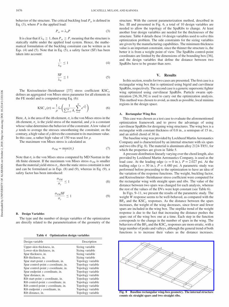
The baselinewing was provided by LockheedMartin AeronauticsCompany and is characterized by an internal structure with six sparsand two ribs (Fig. 8). The material is aluminum alloy 2124-T851, forwhich the properties are given in Table 5.

A pressure distribution linearly varying over the chord length, alsoprovided by Lockheed Martin Aeronautics Company, is used as theload case. At the leading edge (x� 0 in:), P� 2:027 psi. At thetrailing edge (x� 30 in:), P� 4:480 psi. A parametric study wasperformed before proceeding to the optimization to have an idea ofthe variation of the response functions. The weight, buckling factor,and Kreisselmeier–Steinhauser stress coefficient were computed forthe rectangular wing with straight spars and ribs. The value of thedistance between two spars was changed for each analysis, whereasthe rest of the values of the DVs were kept constant (see Table 6).

In Figs. 9–11, we present the results of the parametric study. TheweightW response seems to be well-behaved, as compared with theBF0 and the KSC� responses. As the distance between the sparsincreases, the weight of the wing decreases, since fewer and fewerspars are included in the wing box. The steplike trend of the weightresponse is due to the fact that increasing the distance pushes thespars out of the wing box one at a time. Each step in the functioncorresponds to the change in the number of spars in the wing. Thebehaviors of theBF0 and theKSC� responses are more erratic, with alarge number of peaks and valleys, although the general trend of bothfunctions is to increase their values as the distance increases.

Table 4 Optimization design variables

Design variable Description

Upper-skin thickness, in. Sizing variableLower-skin thickness, in. Sizing variableSpar thickness, in. Sizing variableRib thickness, in. Sizing variableSpar start-point x coordinate, in. Topology variableSpar control-point x coordinate, in. Topology variableSpar control-point y coordinate, in. Topology variableSpar endpoint x coordinate, in. Topology variableSpar distance, in. Topology variableRib start-point y coordinate, in. Topology variableRib control-point x coordinate, in. Topology variableRib control-point y coordinate, in. Topology variableRib endpoint y coordinate, in. Topology variableRib distance, in. Topology variable Fig. 8 Baseline rectangular wing-box geometry. The internal structure

counts six straight spars and two straight ribs.

1676 LOCATELLI, MULANI, AND KAPANIA

Dow

nloa

ded

by U

NIV

ER

SIT

Y O

F A

LA

BA

MA

on

Oct

ober

2, 2

018

| http

://ar

c.ai

aa.o

rg |

DO

I: 1

0.25

14/1

.C03

1336

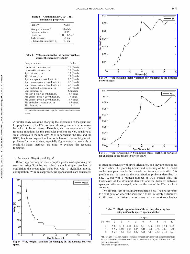
A similar study was done changing the orientation of the spars andkeeping the rest of the DVs constant, showing similar discontinuousbehavior of the responses. Therefore, we can conclude that theresponse functions for this particular problem are very sensitive tosmall changes in the topology DVs; in particular, the BF0 and theKSC� functions display this kind of behavior. This could generateproblems for the optimizer, especially if gradient-based methods orsensitivity-based methods are used to evaluate the responsefunctions.

1. Rectangular Wing Box with Bigrid

Before approaching the more complex problem of optimizing thestructure using SpaRibs, we solved a much simpler problem ofoptimizing the rectangular wing box with a bigridlike internalconfiguration. With this approach, the spars and ribs are considered

as straight structures with fixed orientation, and they are orthogonalto each other. The geometry update and remeshing of the FE modelare less complex than for the case of curvilinear spars and ribs. Thisproblem can be seen as the optimization problem described inSec. IV, but with a reduced number of DVs. Indeed, only thethicknesses of the structural elements and the distances betweenspars and ribs are changed, whereas the rest of the DVs are keptconstant.

Twodifferent sets of results are presented below. Thefirst set refersto a configuration where the spars and ribs are uniformly distributed;in other words, the distance between any two spars next to each other

Table 5 Aluminum alloy 2124 T851

mechanical properties

Property Value

Young’s modulus E 10.6 MsiPoisson’s ratio � 0.33Density � 0:101 lb=in:3

Yield stress �y 64 ksiUltimate tension stress �u 70 ksi

Table 6 Values assumed by the design variables

during the parametric studya

Design variable Value

Upper-skin thickness, in. 0.2 (fixed)Lower-skin thickness, in. 0.2 (fixed)Spar thickness, in. 0.2 (fixed)Rib thickness, in. 0.2 (fixed)Spar start-point x coordinate, in. 2.5 (fixed)Spar control-point x coordinate, in. 2.5 (fixed)Spar control-point y coordinate, in. 7.5 (fixed)Spar endpoint x coordinate, in. 2.5 (fixed)Spar distance, in. ChangingRib start-point y coordinate, in. 1.85 (fixed)Rib control-point x coordinate, in. 15 (fixed)Rib control-point y coordinate, in. 1.85 (fixed)Rib endpoint y coordinate, in. 1.85 (fixed)Rib distance, in. 11.3

aAll variables are constant except for the distance between thespars.

Fig. 9 Wing weight variation for changing in the distance between

spars.

Fig. 10 Wing buckling-factor variation for changing in the distance

between spars.

Fig. 11 Wing Kreisselmeier–Steinhauser stress coefficient variation

for changing in the distance between spars.

Table 7 Bigrid optimization of the rectangular wing box

using uniformly spaced spars and ribsa

No. spars

No. ribs 2 3 4 5 6 7 8 10 12

2 5.61 5.13 4.44 4.12 4.03 4.06 3.82 3.54 3.43b

3 5.56 5.01 4.35 4.35 4.16 3.96 3.95 3.61 3.484 5.24 4.61 4.58 4.47 4.26 4.11 3.93 3.78 3.77

aThe weight of the structure is optimized for configurations with different numbersof spars and ribs. The best results are obtained with 12 spars and two ribs. Theweight is in pounds.bIndicates the lighter structure.

LOCATELLI, MULANI, AND KAPANIA 1677

Dow

nloa

ded

by U

NIV

ER

SIT

Y O

F A

LA

BA

MA

on

Oct

ober

2, 2

018

| http

://ar

c.ai

aa.o

rg |

DO

I: 1

0.25

14/1

.C03

1336

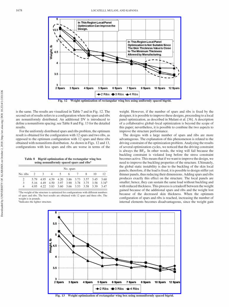
is the same. The results are visualized in Table 7 and in Fig. 12. Thesecond set of results refers to a configuration where the spars and ribsare nonuniformly distributed. An additional DV is introduced todefine a nonuniform spacing; see Table 8 and Fig. 13 for the detailedresults.

For the uniformly distributed spars and ribs problem, the optimumresult is obtained for the configuration with 12 spars and two ribs, asopposed to the optimum configuration with 12 spars and three ribsobtained with nonuniform distribution. As shown in Figs. 12 and 13,configurations with less spars and ribs are worse in terms of the

weight. However, if the number of spars and ribs is fixed by thedesigner, it is possible to improve these designs, proceeding to a localpanel optimization, as described in Mulani et al. [36]. A descriptionof a collaborative global–local optimization is beyond the scope ofthis paper; nevertheless, it is possible to combine the two aspects toimprove the structure performance.

The designs with a large number of spars and ribs are moreadvantageous. The explanation of this phenomenon is related to thedriving constraint of the optimization problem. Analyzing the resultsof several optimization cycles, we noticed that the driving constraintis always the BF0. In other words, the wing will fail because thebuckling constraint is violated long before the stress constraintbecomes active. Thismeans that if wewant to improve the design, weneed to improve the buckling properties of the structure. Ultimately,the global static instability is due to the buckling of the skin localpanels; therefore, if the load is fixed, it is possible to design stiffer yetthinner panels, thus reducing their dimensions. Adding spars and ribsproduces exactly this effect on the structure. The local panels aresmaller; hence, they can sustain the same load without buckling andwith reduced thickness. This process is a tradeoff between theweightgained because of the additional spars and ribs and the weight lostbecause of the decreased skin thickness. When the optimumconfiguration of spars and ribs is reached, increasing the number ofinternal elements becomes disadvantageous, since the weight gain

Fig. 12 Weight optimization of rectangular wing box using uniformly spaced bigrid.

Table 8 Bigrid optimization of the rectangular wing box

using nonuniformly spaced spars and ribsa

No. spars

No. ribs 2 3 4 5 6 7 8 10 12

2 5.79 4.95 4.59 4.20 3.86 3.73 3.57 3.45 3.603 5.16 4.49 4.50 3.97 3.90 3.78 3.75 3.58 3.34b

4 4.95 4.22 3.83 3.60 3.66 3.53 3.58 3.39 3.47

aThe weight of the structure is optimized for configurations with different numbersof spars and ribs. The best results are obtained with 12 spars and three ribs. Theweight is in pounds.bIndicates the lighter structure.

Fig. 13 Weight optimization of rectangular wing box using nonuniformly spaced bigrid.

1678 LOCATELLI, MULANI, AND KAPANIA

Dow

nloa

ded

by U

NIV

ER

SIT

Y O

F A

LA

BA

MA

on

Oct

ober

2, 2

018

| http

://ar

c.ai

aa.o

rg |

DO

I: 1

0.25

14/1

.C03

1336

due to the added structural component is not compensated by theweight reduction due to the reduced skin thickness, leading to anoverall weight increase.

In Table 9, the thickness of the structure is shown for both optimumbigrid configurations found. The minimummanufacturing thicknessof 0.015 in. is reached in almost every part of the skin.

2. Rectangular Wing Box with Curvilinear SpaRibs

The optimization of the rectangular wing box using uniformly andnonuniformly spaced bigrid is the first step toward the imple-mentation of curvilinear SpaRibs. In this section, three sets ofoptimization resultswith SpaRibs are presented. Thefirst two sets are

obtained with the one-step optimization framework, and the third setis obtained by applying the two-step optimization framework.

In Tables 10 and 11, we present the DV vectors of the optimumconfigurations found using the one-step optimization frameworkpresented in Sec. II. These result are obtainedwith PSO optimizationmethod with a population size of five particles. The starting designpoint and some of the side constraints characterizing the boundariesof the DVs are different and account for the different optimumdesigns reached.

Figures 14 and 15 show the internal topology of the optimizedrectangular wing box. The two topologies are completely differentfrom one another and yet their weights are in the same range. Theadvantage of having such different structures with similar bucklingand weight properties is clear if we consider the fact that the

Table 9 Optimal design thicknesses for the rectangular wing

Uniformdistribution

Nonuniformdistribution

Baseline

Upper-skin thickness, in. 0.015 0.032 0.06Lower-skin thickness, in. 0.015 0.015 0.06Spar thickness, in. 0.036 0.015 0.04Rib thickness, in. 0.015 0.015 0.04

Table 10 DV results for the rectangularwing optimized

using curvilinear SpaRibs and one-step optimizationframework: case I

Design variable Optimized Baseline

Upper-skin thickness, in. 0.038 0.06Lower-skin thickness, in. 0.040 0.06Spar thickness, in. 0.015 0.04Rib thickness, in. 0.015 0.04Spar start-point x coordinate, in. 1.871 2.5Spar control-point x coordinate, in. 0.142 2.5Spar control-point y coordinate, in. 3.519 7.5Spar endpoint x coordinate, in. �2:000 2.5Spar distance, in. 4.2065 5.0Rib start-point y coordinate, in. �0:870 1.85Rib control-point x coordinate, in. 21.331 15.0Rib control-point y coordinate, in. 1.026 1.85Rib endpoint y coordinate, in. �1:545 1.85Rib distance, in. 2.000 11.3ResponsesW, lb 4.62 5.91BF0 0.699 0.587KSC� 0.284 N/A

Table 11 DV results for the rectangularwing optimizedusing curvilinear SpaRibs and one-step optimization

framework: case II

Design variable Optimized Baseline

Upper-skin thickness, in. 0.034 0.06Lower-skin thickness, in. 0.037 0.06Spar thickness, in. 0.019 0.04Rib thickness, in. 0.015 0.04Spar start-point x coordinate, in. 5.000 2.5Spar control-point x coordinate, in. 1.500 2.5Spar control-point y coordinate, in. 5.434 7.5Spar endpoint x coordinate, in. 4.612 2.5Spar distance, in. 2.500 5.0Rib start-point y coordinate, in. 3.422 1.85Rib control-point x coordinate, in. 12.000 15.0Rib control-point y coordinate, in. 3.579 1.85Rib endpoint y coordinate, in. 12.500 1.85Rib distance, in. 5.478 11.3ResponsesW, lb 4.19 5.91BF0 0.752 0.587KSC� 0.284 N/A

Fig. 14 Internal structure of rectangular wing optimized using

curvilinear SpaRibs and one-step optimization: case I.

Fig. 15 Internal structure of rectangular wing optimized using

curvilinear SpaRibs and one-step optimization: case II.

LOCATELLI, MULANI, AND KAPANIA 1679

Dow

nloa

ded

by U

NIV

ER

SIT

Y O

F A

LA

BA

MA

on

Oct

ober

2, 2

018

| http

://ar

c.ai

aa.o

rg |

DO

I: 1

0.25

14/1

.C03

1336

deformation and the mode shapes and frequencies of these structuresare different, leading to different dynamic and aeroelastic behaviors.

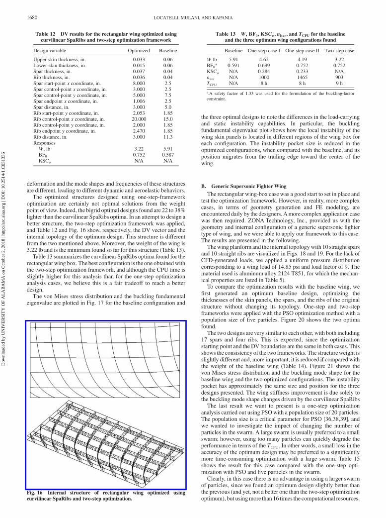
The optimized structures designed using one-step-frameworkoptimization are certainly not optimal solutions from the weightpoint of view. Indeed, the bigrid optimal designs found are 22 to 38%lighter than the curvilinear SpaRibs optima. In an attempt to design abetter structure, the two-step optimization framework was applied,and Table 12 and Fig. 16 show, respectively, the DV vector and theinternal topology of the optimum design. This structure is differentfrom the two mentioned above. Moreover, the weight of the wing is3.22 lb and is the minimum found so far for this structure (Table 13).

Table 13 summarizes the curvilinear SpaRibs optima found for therectangular wing box. The best configuration is the one obtainedwiththe two-step optimization framework, and although the CPU time isslightly higher for this analysis than for the one-step optimizationanalysis cases, we believe this is a fair tradeoff to reach a betterdesign.

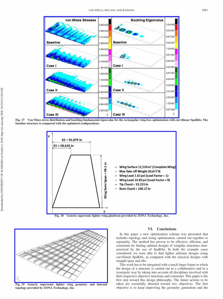
The von Mises stress distribution and the buckling fundamentaleigenvalue are plotted in Fig. 17 for the baseline configuration and

the three optimal designs to note the differences in the load-carryingand static instability capabilities. In particular, the bucklingfundamental eigenvalue plot shows how the local instability of thewing skin panels is located in different regions of the wing box foreach configuration. The instability pocket size is reduced in theoptimized configurations, when compared with the baseline, and itsposition migrates from the trailing edge toward the center of thewing.

B. Generic Supersonic Fighter Wing

The rectangular wing-box case was a good start to set in place andtest the optimization framework. However, in reality, more complexcases, in terms of geometry generation and FE modeling, areencountered daily by the designers. Amore complex application casewas then required. ZONA Technology, Inc., provided us with thegeometry and internal configuration of a generic supersonic fightertype of wing, and we were able to apply our framework to this case.The results are presented in the following.

Thewing planform and the internal topologywith 10 straight sparsand 10 straight ribs are visualized in Figs. 18 and 19. For the lack ofCFD-generated loads, we applied a uniform pressure distributioncorresponding to a wing load of 14.85 psi and load factor of 9. Thematerial used is aluminum alloy 2124 T851, for which the mechan-ical properties are listed in Table 5).

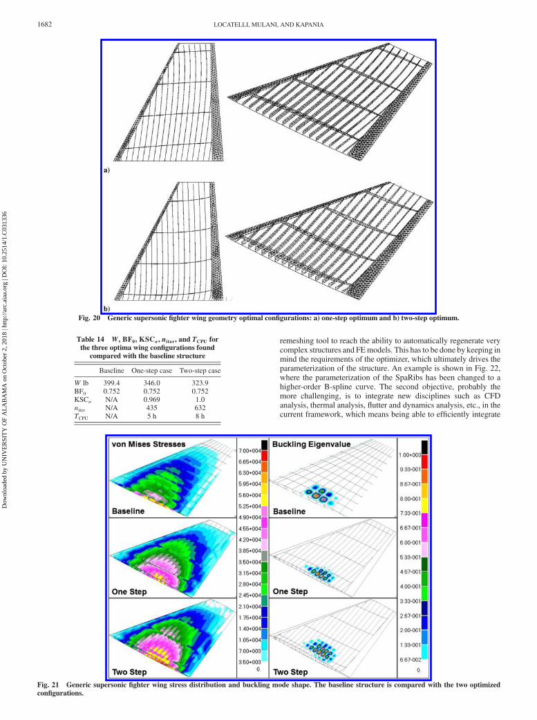
To compare the optimization results with the baseline wing, wefirst generated an optimum baseline design, optimizing thethicknesses of the skin panels, the spars, and the ribs of the originalstructure without changing its topology. One-step and two-stepframeworks were applied with the PSO optimization method with apopulation size of five particles. Figure 20 shows the two optimafound.

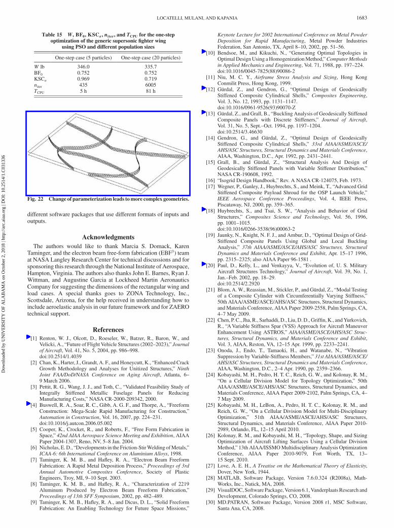
The two designs are very similar to each other, with both including17 spars and four ribs. This is expected, since the optimizationstarting point and the DV boundaries are the same in both cases. Thisshows the consistency of the two frameworks. The structureweight isslightly different and, more important, it is reduced if compared withthe weight of the baseline wing (Table 14). Figure 21 shows thevon Mises stress distribution and the buckling mode shape for thebaseline wing and the two optimized configurations. The instabilitypocket has approximately the same size and position for the threedesigns presented. The wing stiffness improvement is due solely tothe buckling mode shape changes driven by the curvilinear SpaRibs

The last result we want to present is a one-step optimizationanalysis carried out using PSOwith a population size of 20 particles.The population size is a critical parameter for PSO [36,38,39], andwe wanted to investigate the impact of changing the number ofparticles in the swarm. A large swarm is usually preferred to a smallswarm; however, using too many particles can quickly degrade theperformance in terms of the TCPU. In other words, a small loss in theaccuracy of the optimum design may be preferred to a significantlymore time-consuming optimization with a large swarm. Table 15shows the result for this case compared with the one-step opti-mization with PSO and five particles in the swarm.

Clearly, in this case there is no advantage in using a larger swarmof particles, since we found an optimum design slightly better thanthe previous (and yet, not a better one than the two-step optimizationoptimum), but usingmore than 16 times the computational resources.

Table 12 DV results for the rectangular wing optimized using

curvilinear SpaRibs and two-step optimization framework

Design variable Optimized Baseline

Upper-skin thickness, in. 0.033 0.06Lower-skin thickness, in. 0.015 0.06Spar thickness, in. 0.037 0.04Rib thickness, in. 0.036 0.04Spar start-point x coordinate, in. 8.000 2.5Spar control-point x coordinate, in. 3.000 2.5Spar control-point y coordinate, in. 5.000 7.5Spar endpoint x coordinate, in. 1.006 2.5Spar distance, in. 3.000 5.0Rib start-point y coordinate, in. 2.053 1.85Rib control-point x coordinate, in. 20.000 15.0Rib control-point y coordinate, in. 2.000 1.85Rib endpoint y coordinate, in. 2.470 1.85Rib distance, in. 3.000 11.3ResponsesW, lb 3.22 5.91BF0 0.752 0.587KSC� N/A N/A

Fig. 16 Internal structure of rectangular wing optimized using

curvilinear SpaRibs and two-step optimization.

Table 13 W, BF0,KSC� , niter, and TCPU for the baseline

and the three optimum wing configurations found

Baseline One-step case I One-step case II Two-step case

W lb 5.91 4.62 4.19 3.22BF0

a 0.591 0.699 0.752 0.752KSC� N/A 0.284 0.233 N/Aniter N/A 1000 1465 903TCPU N/A 8 h 8 h 9 h

a.A safety factor of 1.33 was used for the formulation of the buckling-factorconstraint.

1680 LOCATELLI, MULANI, AND KAPANIA

Dow

nloa

ded

by U

NIV

ER

SIT

Y O

F A

LA

BA

MA

on

Oct

ober

2, 2

018

| http

://ar

c.ai

aa.o

rg |

DO

I: 1

0.25

14/1

.C03

1336

VI. Conclusions

In this paper a new optimization schema was presented thatincludes topology and sizing optimization, carried out together orseparately. The method has proven to be effective, efficient, andconsistent for finding optimal designs of winglike structures char-acterized by the use of SpaRibs. In both the example casesconsidered, we were able to find lighter airframe designs usingcurvilinear SpaRibs, as compared with the classical designs withstraight spars and ribs.

This work has to be integrated with a much larger frame in whichthe design of a structure is carried out in a collaborative and in asynergetic way by taking into account all disciplines involved withtheir respective objective functions and constraint. This paper is thefirst step toward this design philosophy. The future actions to betaken are essentially directed toward two objectives. The firstobjective is to keep improving the geometry generation and the

Fig. 17 Von Mises stress distribution and buckling fundamental eigenvalue for the rectangular wing-box optimization with curvilinear SpaRibs. The

baseline structure is compared with the optimized configurations.

Fig. 18 Generic supersonic fighter wing planform provided by ZONA Technology, Inc.

Fig. 19 Generic supersonic fighter wing geometry and internal

topology provided by ZONA Technology, Inc.

LOCATELLI, MULANI, AND KAPANIA 1681

Dow

nloa

ded

by U

NIV

ER

SIT

Y O

F A

LA

BA

MA

on

Oct

ober

2, 2

018

| http

://ar

c.ai

aa.o

rg |

DO

I: 1

0.25

14/1

.C03

1336

remeshing tool to reach the ability to automatically regenerate verycomplex structures and FEmodels. This has to be done by keeping inmind the requirements of the optimizer, which ultimately drives theparameterization of the structure. An example is shown in Fig. 22,where the parameterization of the SpaRibs has been changed to ahigher-order B-spline curve. The second objective, probably themore challenging, is to integrate new disciplines such as CFDanalysis, thermal analysis, flutter and dynamics analysis, etc., in thecurrent framework, which means being able to efficiently integrate

Fig. 20 Generic supersonic fighter wing geometry optimal configurations: a) one-step optimum and b) two-step optimum.

Fig. 21 Generic supersonic fighter wing stress distribution and buckling mode shape. The baseline structure is compared with the two optimized

configurations.

Table 14 W, BF0, KSC� , niter, and TCPU for

the three optima wing configurations foundcompared with the baseline structure

Baseline One-step case Two-step case

W lb 399.4 346.0 323.9BF0 0.752 0.752 0.752KSC� N/A 0.969 1.0niter N/A 435 632TCPU N/A 5 h 8 h

1682 LOCATELLI, MULANI, AND KAPANIA

Dow

nloa

ded

by U

NIV

ER

SIT

Y O

F A

LA

BA

MA

on

Oct

ober

2, 2

018

| http

://ar

c.ai

aa.o

rg |

DO

I: 1

0.25

14/1

.C03

1336

different software packages that use different formats of inputs andoutputs.

Acknowledgments

The authors would like to thank Marcia S. Domack, KarenTaminger, and the electron beam free-form fabrication (EBF3) teamat NASA Langley Research Center for technical discussions and forsponsoring this research through the National Institute of Aerospace,Hampton, Virginia. The authors also thanks John E. Barnes, Ryan J.Wittman, and Augustine Garcia at Lockheed Martin AeronauticsCompany for suggesting the dimensions of the rectangular wing andload cases. A special thanks goes to ZONA Technology, Inc.,Scottsdale, Arizona, for the help received in understanding how toinclude aeroelastic analysis in our future framework and for ZAEROtechnical support.

References

[1] Renton, W. J., Olcott, D., Roeseler, W., Batzer, R., Baron, W., andVelicki, A., “Future of Flight Vehicle Structures (2002–2023),” Journalof Aircraft, Vol. 41, No. 5, 2004, pp. 986–998.doi:10.2514/1.4039

[2] Chan, K., Harter, J., Grandt, A. F., andHoneycutt, K., “Enhanced CrackGrowth Methodology and Analyses for Unitized Structures,” Ninth

Joint FAA/DoD/NASA Conference on Aging Aircraft, Atlanta, 6–9 March 2006.

[3] Pettit, R. G., Wang, J. J., and Toth, C., “Validated Feasibility Study ofIntegrally Stiffened Metallic Fuselage Panels for ReducingManufacturing Costs,” NASA CR-2000-209342, 2000.

[4] Buswell, R. A., Soar, R. C., Gibb, A. G. F., and Thorpe, A., “FreeformConstruction: Mega-Scale Rapid Manufacturing for Construction,”Automation in Construction, Vol. 16, 2007, pp. 224–231.doi:10.1016/j.autcon.2006.05.002

[5] Cooper, K., Crocket, R., and Roberts, F., “Free Form Fabrication inSpace,” 42nd AIAA Aerospace Science Meeting and Exhibition, AIAAPaper 2004-1307, Reno, NV, 5–8 Jan. 2004.

[6] Nicholas, E.D., “Developments in the Friction-StirWelding ofMetals,”ICAA-6: 6th International Conference on Aluminium Alloys, 1998.

[7] Taminger, K. M. B., and Hafley, R. A., “Electron Beam FreeformFabrication: A Rapid Metal Deposition Process,” Proceedings of 3rdAnnual Automotive Composites Conference, Society of PlasticEngineers, Troy, MI, 9–10 Sept. 2003.

[8] Taminger, K. M. B., and Hafley, R. A., “Characterization of 2219Aluminum Produced by Electron Beam Freeform Fabrication,”Proceedings of 13th SFF Symposium, 2002, pp. 482–489.

[9] Taminger, K. M. B., Hafley, R. A., and Dicus, D. L., “Solid FreeformFabrication: An Enabling Technology for Future Space Missions,”

Keynote Lecture for 2002 International Conference on Metal Powder

Deposition for Rapid Manufacturing, Metal Powder IndustriesFederation, San Antonio, TX, April 8–10, 2002, pp. 51–56.

[10] Bendsoe, M., and Kikuchi, N., “Generating Optimal Topologies inOptimal DesignUsing aHomogenizationMethod,”ComputerMethods

in Applied Mechanics and Engineering, Vol. 71, 1988, pp. 197–224.doi:10.1016/0045-7825(88)90086-2

[11] Niu, M. C. Y., Airframe Stress Analysis and Sizing, Hong KongConmilit Press, Hong Kong, 1999.

[12] Gürdal, Z., and Gendron, G., “Optimal Design of GeodesicallyStiffened Composite Cylindrical Shells,” Composites Engineering,Vol. 3, No. 12, 1993, pp. 1131–1147.doi:10.1016/0961-9526(93)90070-Z

[13] Gürdal, Z., and Grall, B., “Buckling Analysis of Geodesically StiffenedComposite Panels with Discrete Stiffeners,” Journal of Aircraft,Vol. 31, No. 5, Sept.–Oct. 1994, pp. 1197–1204.doi:10.2514/3.46630

[14] Gendron, G., and Gürdal, Z., “Optimal Design of GeodesicallyStiffened Composite Cylindrical Shells,” 33rd AIAA/ASME/ASCE/

AHS/ASC Structures, Structural Dynamics and Materials Conference,AIAA, Washington, D.C., Apr. 1992, pp. 2431–2441.

[15] Grall, B., and Gürdal, Z., “Structural Analysis And Design ofGeodesically Stiffened Panels with Variable Stiffener Distribution,”NASA CR-190608, 1992.

[16] “Isogrid Design Handbook,” Rev. A NASA CR-124075, Feb. 1973.[17] Wegner, P., Ganley, J., Huybrechts, S., and Meink, T., “Advanced Grid

Stiffened Composite Payload Shroud for the OSP Launch Vehicle,”IEEE Aerospace Conference Proceedings, Vol. 4, IEEE Press,Piscataway, NJ, 2000, pp. 359–365.

[18] Huybrechts, S., and Tsai, S. W., “Analysis and Behavior of GridStructures,” Composites Science and Technology, Vol. 56, 1996,pp. 1001–1015.doi:10.1016/0266-3538(96)00063-2

[19] Jaunky, N., Knight, N. F. J., and Ambur, D., “Optimal Design of Grid-Stiffened Composite Panels Using Global and Local BucklingAnalysis,” 37th AIAA/ASME/ASCE/AHS/ASC Structures, Structural

Dynamics and Materials Conference and Exhibit, Apr. 15–17 1996,pp. 2315–2325; also AIAA Paper 96-1581 .

[20] Paul, D., Kelly, L., and Venkayya, V., “Evolution of, U. S. MilitaryAircraft Structures Technology,” Journal of Aircraft, Vol. 39, No. 1,Jan.–Feb. 2002, pp. 18–29.doi:10.2514/2.2920

[21] Blom, A.W., Reassian, M., Stickler, P., and Gürdal, Z., “Modal Testingof a Composite Cylinder with Circumferentially Varying Stiffness,”50th AIAA/ASME/ASCE/AHS/ASC Structures, Structural Dynamics,andMaterials Conference, AIAA Paper 2009-2558, Palm Springs, CA,4–7 May 2009.

[22] Chen, P. C., Jha, R., Sarhaddi,D., Liu,D.D., Griffin,K., andYurkovich,R., “AVariable Stiffness Spar (VSS) Approach for Aircraft ManeuverEnhancement Using ASTROS,” AIAA/ASME/ASCE/AHS/ASC Struc-

tures, Structural Dynamics, and Materials Conference and Exhibit,Vol. 3, AIAA, Reston, VA, 12–15 Apr. 1999, pp. 2233–2241.

[23] Onoda, J., Endo, T., Tamaoki, H., and Watanabe, N., “VibrationSuppression by Variable-Stiffness Members,” 31st AIAA/ASME/ASCE/

AHS/ASC Structures, Structural Dynamics and Materials Conference,AIAA, Washington, D.C., 2–4 Apr. 1990, pp. 2359–2366.

[24] Kobayashi, M. H., Pedro, H. T. C., Reich, G. W., and Kolonay, R. M.,“On a Cellular Division Model for Topology Optimization,” 50thAIAA/ASME/ASCE/AHS/ASC Structures, Structural Dynamics, andMaterials Conference, AIAA Paper 2009-2102, Palm Springs, CA, 4–7 May 2009.

[25] Kobayashi, M. H., LeBon, A., Pedro, H. T. C., Kolonay, R. M., andReich, G. W., “On a Cellular Division Model for Multi-DisciplinaryOptimization,” 51th AIAA/ASME/ASCE/AHS/ASC Structures,Structural Dynamics, and Materials Conference, AIAA Paper 2010-2989, Orlando, FL, 12–15 April 2010.

[26] Kolonay, R. M., and Kobayashi, M. H., “Topology, Shape, and SizingOptimization of Aircraft Lifting Surfaces Using a Cellular DivisionMethod,” 13th AIAA/ISSMOMultidisciplinary Analysis OptimizationConference, AIAA Paper 2010-9079, Fort Worth, TX, 13–15 Sept. 2010.

[27] Love, A. E. H., A Treatise on the Mathematical Theory of Elasticity,Dover, New York, 1944.

[28] MATLAB, Software Package, Version 7.6.0.324 (R2008a), Math-Works, Inc., Natick, MA, 2008.

[29] VisualDOC, Software Package,Version 6.1,VanderplaatsResearch andDevelopment, Colorado Springs, CO, 2008.

[30] MD.PATRAN, Software Package, Version 2008 r1, MSC Software,Santa Ana, CA, 2008.

Fig. 22 Change of parameterization leads tomore complex geometries.

Table 15 W, BF0,KSC� , niter, and TCPU for the one-step

optimization of the generic supersonic fighter wing

using PSO and different population sizes

One-step case (5 particles) One-step case (20 particles)

W lb 346.0 335.7BF0 0.752 0.752KSC� 0.969 0.719niter 435 6005TCPU 5 h 81 h

LOCATELLI, MULANI, AND KAPANIA 1683

Dow

nloa

ded

by U

NIV

ER

SIT

Y O

F A

LA

BA

MA

on

Oct

ober

2, 2

018

| http

://ar

c.ai

aa.o

rg |

DO

I: 1

0.25

14/1

.C03

1336

[31] MD.NASTRAN, Software Package, Version R2.1, MSC Software,Santa Ana, CA, 2008.

[32] Gurav, S. P., and Kapania, R. K., “Development of Framework for theDesign Optimization of Unitized Structures,” 50th AIAA/ASME/ASCE/AHS/ASC Structures, Structural Dynamics, and MaterialsConference, AIAA Paper 2009-2186, Palm Springs, CA, 4–7 May 2009.

[33] Schramm, U., Zhou, M., Tang, P. S., and Harte, C., “Topology Layoutfor Structural Designs and Buckling,” 10th AIAA/ISSMO Multi-disciplinaryAnalysis andOptimizationConference, AIAAPaper 2004-4636, Albany, NY, Aug. 30–Sept. 1 2004.

[34] Mulani, S. B., Li, J., Joshi, P., and Kapania, R. K., “Optimization ofStiffened Electron Beam Freeform Fabrication (EBF3) Panels UsingResponse Surface Approaches,” 48th AIAA/ASME/ASCE/AHS/ASCStructures, Structural Dynamics and Materials Conference, AIAAPaper 2007-1901, Honolulu, 23–26 April 2007.

[35] Mulani, S. B., Joshi, P., Li, J., Kapania, R. K., and Shin, Y., “OptimalDesign of Unitized Structures with Curvilinear Stiffeners UsingResponse Surface Approaches,” Journal of Aircraft, Vol. 47, No. 6,

Nov.–Dec. 2010, pp. 1898–1906.doi:10.2514/1.47411

[36] Mulani, S. B., Locatelli, D., and Kapania, R. K., “AlgorithmDevelopment for Optimization of Arbitrary Geometry Panels UsingCurvilinear Stiffeners,” 51st AIAA/ASME/ASCE/AHS/ASC Struc-tures, Structural Dynamics and Materials Conference, AIAAPaper 2010-2674, 10–15 April 2010.

[37] Kreisselmeier, G., and Steinhauser, R., “Systematic Control Design byOptimizing a Vector Performance Index,” Proceedings of the IFAC

Symposium on Computer-Aided Design of Control Systems, Zurich,1979, pp. 113–117.

[38] Venter, G., and Sobieszczanski-Sobieski, J., “MultidisciplinaryOptimization of a Transport Aircraft Wing Using Particle SwarmOptimization,” 9th AIAA/ISSMO Symposium on MultidisciplinaryAnalysis and Optimization, AIAA Paper 2002-644, Atlanta, 4–6 Sept. 2002.

[39] Venter, G., and Sobieszczanski-Sobieski, J., “Particle SwarmOptimization,” AIAA Journal, Vol. 41, No. 8, 2003, pp. 1583–1589.doi:10.2514/2.2111

1684 LOCATELLI, MULANI, AND KAPANIA

Dow

nloa

ded

by U

NIV

ER

SIT

Y O

F A

LA

BA

MA

on

Oct

ober

2, 2

018

| http

://ar

c.ai

aa.o

rg |

DO

I: 1

0.25

14/1

.C03

1336

This article has been cited by:

1. Ramana V. Grandhi, Hao Li, Marcelo Kobayashi, Raymond M. Kolonay. Vehicle Configuration Design Using Cellular-Division and Level-Set Based Topology Optimization 29-40. [Crossref]

2. Gunther Moors, Christos Kassapoglou, Sergio Frascino Müller de Almeida, Clovis Augusto Eça Ferreira. 2018. Weighttrades in the design of a composite wing box: effect of various design choices. CEAS Aeronautical Journal 4. . [Crossref]

3. Mohammad Raheel, Vassili Toropov. Topology Optimization of an Aircraft Wing with an Outboard X-Stabilizer .[Citation] [PDF] [PDF Plus]

4. Max M. Opgenoord, Karen E. Willcox. Aeroelastic Tailoring using Additively Manufactured Lattice Structures . [Citation][PDF] [PDF Plus]

5. Rikin Gupta, Nathan J. Love, Rakesh K. Kapania, David Schmidt. Development of Longitudinal Flight Dynamics AnalysisFramework with Controllability and Observability Metrics . [Citation] [PDF] [PDF Plus]

6. Wei Zhao, Rakesh K. Kapania. Multiobjective Optimization of Composite Flying-wings with SpaRibs and MultipleControl Surfaces . [Citation] [PDF] [PDF Plus]

7. Scott Townsend, Bret Stanford, Sandilya Kambampati, Hyunsun A. Kim. Aeroelastic Optimization of Wing Skin usinga Level Set Method . [Citation] [PDF] [PDF Plus]

8. Bret K. Stanford. 2018. Aeroelastic Wingbox Stiffener Topology Optimization. Journal of Aircraft 55:3, 1244-1251.[Abstract] [Full Text] [PDF] [PDF Plus]

9. Arthur Dubois, Charbel Farhat, Abdullah H. Abukhwejah, Hesham Mohamed Shageer. 2018. Parameterization Frameworkfor the MDAO of Wing Structural Layouts. AIAA Journal 56:4, 1627-1638. [Abstract] [Full Text] [PDF] [PDF Plus]

10. Zhijun Liu, Shingo Cho, Akihiro Takezawa, Xiaopeng Zhang, Mitsuru Kitamura. 2018. Two-stage layout–sizeoptimization method for prow stiffeners. International Journal of Naval Architecture and Ocean Engineering . [Crossref]

11. Elliot K. Bontoft, Vassili Toropov. Topology Optimisation of Multi-Element Wingtip Devices . [Citation] [PDF] [PDFPlus]

12. Bret Stanford, Christine V. Jutte, Christian Coker. Sizing and Layout Design of an Aeroelastic Wingbox through NestedOptimization . [Citation] [PDF] [PDF Plus]

13. Wei Zhao, Rakesh K. Kapania. BLP Optimization of Composite Flying-wings with SpaRibs and Multiple ControlSurfaces . [Citation] [PDF] [PDF Plus]

14. Sandilya Kambampati, Scott Townsend, Hyunsun A. Kim. Aeroelastic Level Set Topology Optimization for a 3D Wing .[Citation] [PDF] [PDF Plus]

15. David J. Munk, Dries Verstraete, Gareth A. Vio. 2017. Effect of fluid-thermal–structural interactions on the topologyoptimization of a hypersonic transport aircraft wing. Journal of Fluids and Structures 75, 45-76. [Crossref]

16. Weizhu Yang, Zhufeng Yue, Lei Li, Fan Yang, Peiyan Wang. 2017. Optimization design of unitized panels with stiffenersin different formats using the evolutionary strategy with covariance matrix adaptation. Proceedings of the Institution ofMechanical Engineers, Part G: Journal of Aerospace Engineering 231:9, 1563-1573. [Crossref]

17. Bret Stanford. Aeroelastic Wingbox Stringer Topology Optimization . [Citation] [PDF] [PDF Plus]18. Mohamed Jrad, Shuvodeep De, Rakesh K. Kapania. Global-local Aeroelastic Optimization of Internal Structure of

Transport Aircraft wing . [Citation] [PDF] [PDF Plus]19. X.C. Qin, C.Y. Dong, F. Wang, X.Y. Qu. 2017. Static and dynamic analyses of isogeometric curvilinearly stiffened plates.

Applied Mathematical Modelling 45, 336-364. [Crossref]20. Wei Zhao, Rakesh K. Kapania. 2017. Vibration Analysis of Curvilinearly Stiffened Composite Panel Subjected to In-Plane

Loads. AIAA Journal 55:3, 981-997. [Abstract] [Full Text] [PDF] [PDF Plus]21. John T. Hwang, Joaquim R.R.A. Martins. 2016. An unstructured quadrilateral mesh generation algorithm for aircraft

structures. Aerospace Science and Technology 59, 172-182. [Crossref]22. Qiang Liu, Mohamed Jrad, Sameer B. Mulani, Rakesh K. Kapania. 2016. Global/Local Optimization of Aircraft Wing

Using Parallel Processing. AIAA Journal 54:11, 3338-3348. [Abstract] [Full Text] [PDF] [PDF Plus]23. Peng Hao, Bo Wang, Kuo Tian, Gang Li, Xi Zhang. 2016. Optimization of Curvilinearly Stiffened Panels with Single

Cutout Concerning the Collapse Load. International Journal of Structural Stability and Dynamics 16:07, 1550036. [Crossref]

Dow

nloa

ded

by U

NIV

ER

SIT

Y O

F A

LA

BA

MA

on

Oct

ober

2, 2

018

| http

://ar

c.ai

aa.o

rg |

DO

I: 1

0.25

14/1

.C03

1336

24. Teemu J. Ikonen, Andras Sobester. Ground Structure Approaches for the Evolutionary Optimization of Aircraft WingStructures . [Citation] [PDF] [PDF Plus]

25. P. Hao, B. Wang, K. Tian, G. Li, K. Du, F. Niu. 2016. Efficient Optimization of Cylindrical Stiffened Shells with ReinforcedCutouts by Curvilinear Stiffeners. AIAA Journal 54:4, 1350-1363. [Abstract] [Full Text] [PDF] [PDF Plus]

26. Guillaume Francois, Jonathan E. Cooper, Paul Weaver. Impact of the Wing Sweep Angle and Rib Orientation on WingStructural Response for Un-Tapered Wings . [Citation] [PDF] [PDF Plus]

27. Arthur Dubois, Charbel Farhat, Abdullah H. Abukhwejah. Parameterization Framework for Aeroelastic DesignOptimization of Bio-Inspired Wing Structural Layout . [Citation] [PDF] [PDF Plus]

28. Wei Zhao, Rakesh K. Kapania. Vibrational Analysis of Unitized Curvilinearly Stiffened Composite Panels Subjected to In-plane Loads . [Citation] [PDF] [PDF Plus]

29. Wei Zhao, Rakesh K. Kapania. 2016. Buckling analysis of unitized curvilinearly stiffened composite panels. CompositeStructures 135, 365-382. [Crossref]

30. Shutian Liu, Quhao Li, Wenjiong Chen, Rui Hu, Liyong Tong. 2015. H-DGTP—a Heaviside-function based directionalgrowth topology parameterization for design optimization of stiffener layout and height of thin-walled structures. Structuraland Multidisciplinary Optimization 52:5, 903-913. [Crossref]

31. Bret K. Stanford, Peter D. Dunning. 2015. Optimal Topology of Aircraft Rib and Spar Structures Under AeroelasticLoads. Journal of Aircraft 52:4, 1298-1311. [Abstract] [Full Text] [PDF] [PDF Plus]

32. Robert E. Bartels, Pawel Chwalowski, Christie Funk, Jennifer Heeg, Jiyoung Hur, Mark D. Sanetrik, Robert C.Scott, Walter A. Silva, Bret Stanford, Carol D. Wieseman. Ongoing Fixed Wing Research within the NASA LangleyAeroelasticity Branch . [Citation] [PDF] [PDF Plus]

33. Davide Locatelli, Sameer B. Mulani, Rakesh K. Kapania. 2014. Parameterization of Curvilinear Spars and Ribs for OptimumWing Structural Design. Journal of Aircraft 51:2, 532-546. [Abstract] [Full Text] [PDF] [PDF Plus]

Dow

nloa

ded

by U

NIV

ER

SIT

Y O

F A

LA

BA

MA

on

Oct

ober

2, 2

018

| http

://ar

c.ai

aa.o

rg |

DO

I: 1

0.25

14/1

.C03

1336

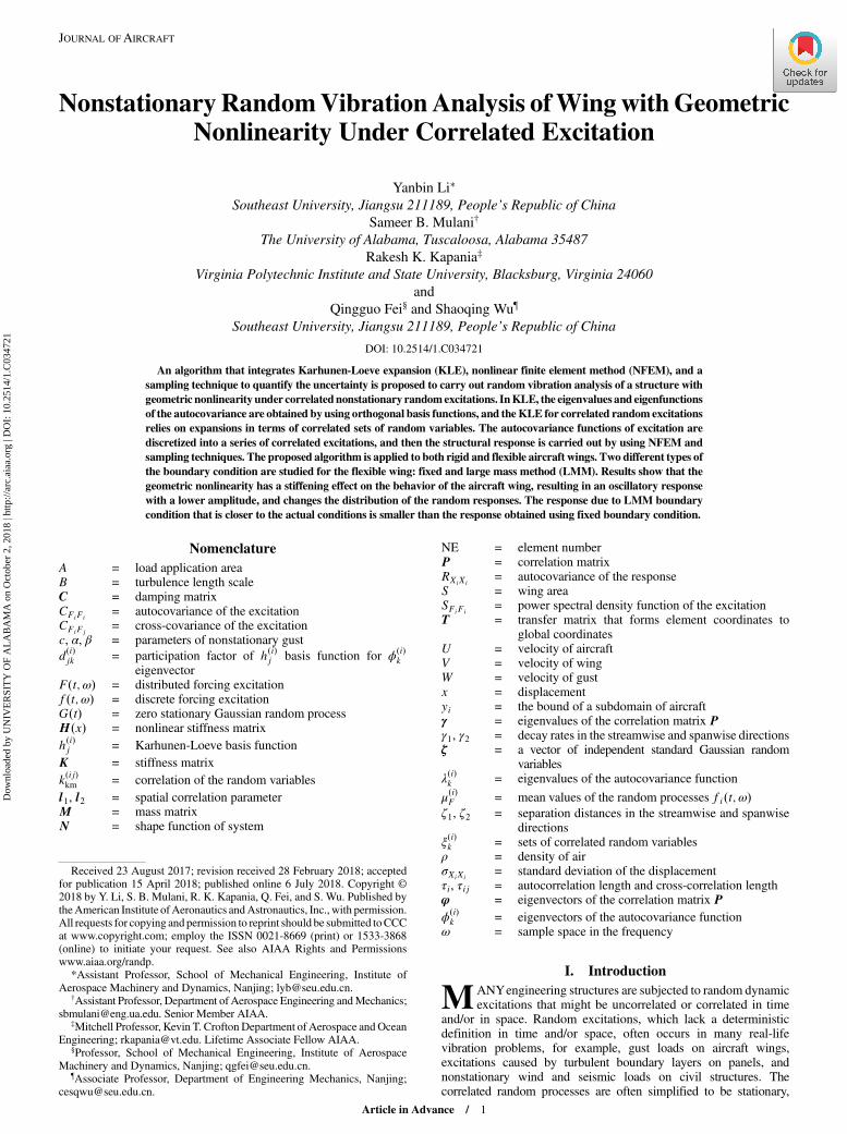
NonstationaryRandomVibration Analysis ofWingwithGeometricNonlinearity Under Correlated Excitation

Yanbin Li∗

Southeast University, Jiangsu 211189, People’s Republic of China

Sameer B. Mulani†

The University of Alabama, Tuscaloosa, Alabama 35487

Rakesh K. Kapania‡

Virginia Polytechnic Institute and State University, Blacksburg, Virginia 24060

and

Qingguo Fei§ and Shaoqing Wu¶

Southeast University, Jiangsu 211189, People’s Republic of China

DOI: 10.2514/1.C034721

An algorithm that integrates Karhunen-Loeve expansion (KLE), nonlinear finite element method (NFEM), and a

sampling technique to quantify the uncertainty is proposed to carry out random vibration analysis of a structure with

geometric nonlinearity under correlatednonstationary randomexcitations. InKLE, the eigenvalues and eigenfunctions

of the autocovariance are obtained by using orthogonal basis functions, and theKLE for correlated random excitations

relies on expansions in terms of correlated sets of random variables. The autocovariance functions of excitation are

discretized into a series of correlated excitations, and then the structural response is carried out by using NFEM and

sampling techniques. The proposed algorithm is applied to both rigid and flexible aircraft wings. Two different types of

the boundary condition are studied for the flexible wing: fixed and large mass method (LMM). Results show that the

geometric nonlinearity has a stiffening effect on the behavior of the aircraft wing, resulting in an oscillatory response

with a lower amplitude, and changes the distribution of the random responses. The response due to LMM boundary

condition that is closer to the actual conditions is smaller than the response obtained using fixed boundary condition.

Nomenclature

A = load application areaB = turbulence length scaleC = damping matrixCFiFi

= autocovariance of the excitationCFiFj

= cross-covariance of the excitationc, α, β = parameters of nonstationary gust

d�i�jk = participation factor of h�i�j basis function for ϕ�i�k

eigenvectorF�t;ω� = distributed forcing excitationf�t;ω� = discrete forcing excitationG�t� = zero stationary Gaussian random processH�x� = nonlinear stiffness matrix

h�i�j = Karhunen-Loeve basis function

K = stiffness matrix

k�ij�km = correlation of the random variables

l1, l2 = spatial correlation parameterM = mass matrixN = shape function of system

NE = element numberP = correlation matrixRXiXi

= autocovariance of the responseS = wing areaSFiFi

= power spectral density function of the excitationT = transfer matrix that forms element coordinates to

global coordinatesU = velocity of aircraftV = velocity of wingW = velocity of gustx = displacementyi = the bound of a subdomain of aircraftγ = eigenvalues of the correlation matrix Pγ1, γ2 = decay rates in the streamwise and spanwise directionsζ = a vector of independent standard Gaussian random

variablesλ�i�k = eigenvalues of the autocovariance function

μ�i�F = mean values of the random processes fi�t;ω�ζ1, ζ2 = separation distances in the streamwise and spanwise

directionsξ�i�k = sets of correlated random variablesρ = density of airσXiXi

= standard deviation of the displacementτi, τij = autocorrelation length and cross-correlation lengthφ = eigenvectors of the correlation matrix P

ϕ�i�k = eigenvectors of the autocovariance function

ω = sample space in the frequency

I. Introduction

M ANYengineering structures are subjected to random dynamicexcitations that might be uncorrelated or correlated in time

and/or in space. Random excitations, which lack a deterministicdefinition in time and/or space, often occurs in many real-lifevibration problems, for example, gust loads on aircraft wings,excitations caused by turbulent boundary layers on panels, andnonstationary wind and seismic loads on civil structures. Thecorrelated random processes are often simplified to be stationary,

Received 23 August 2017; revision received 28 February 2018; acceptedfor publication 15 April 2018; published online 6 July 2018. Copyright ©2018 by Y. Li, S. B. Mulani, R. K. Kapania, Q. Fei, and S. Wu. Published bytheAmerican Institute ofAeronautics andAstronautics, Inc., with permission.All requests for copying and permission to reprint should be submitted toCCCat www.copyright.com; employ the ISSN 0021-8669 (print) or 1533-3868(online) to initiate your request. See also AIAA Rights and Permissionswww.aiaa.org/randp.

*Assistant Professor, School of Mechanical Engineering, Institute ofAerospace Machinery and Dynamics, Nanjing; lyb@seu.edu.cn.

†Assistant Professor, Department of Aerospace Engineering andMechanics;sbmulani@eng.ua.edu. Senior Member AIAA.

‡Mitchell Professor, Kevin T. Crofton Department of Aerospace andOceanEngineering; rkapania@vt.edu. Lifetime Associate Fellow AIAA.

§Professor, School of Mechanical Engineering, Institute of AerospaceMachinery and Dynamics, Nanjing; qgfei@seu.edu.cn.

¶Associate Professor, Department of Engineering Mechanics, Nanjing;cesqwu@seu.edu.cn.

Article in Advance / 1

JOURNAL OF AIRCRAFT

Dow

nloa

ded

by U

NIV

ER

SIT

Y O

F A

LA

BA

MA

on

Oct

ober

2, 2

018

| http

://ar

c.ai

aa.o

rg |

DO

I: 1

0.25

14/1

.C03

4721

Gaussian, and uncorrelated processes for the convenience of a randomvibration analysis. However, many engineering structures encounternonstationary and correlated random excitations.Most of the previous studies on random vibration were confined

to linear systems that are restricted to small deformations wheregeometric nonlinearities were not considered for larger complexsystems [1]. It is necessary to consider geometric nonlinear effects toget the realistic behavior of the structures where large deformationoccurs. For flexible structures such as aircraft, satellites, bridges, andtall/slender structures, the large out-of-plane deformation results in thepresence of in-plane stretching.Hence, nonlinearitiesmay significantlychange the dynamic structural response behavior. Moreover, nonlinearrandom vibration analysis has been drawing increasing attention inrecent years to designmany civil,mechanical, and aerospace structures[2].However, nonlinear randomvibration analysis under nonstationarycorrelated random processes has not been studied in great depth. Thenonlinear random vibration analysis is conducted by analytical andnumericalmethods [3].Analyticalmethodshave been used to carry outthe nonlinear random vibration analysis under nonstationary randomexcitations [4–6] for simple systems. For large complex systems,the development of nonlinear random vibration analysis undernonstationary correlated excitations is inhibited by both the extensivecomputational cost and the inherentmathematical intricacies.With therelentless progress in high-performance computing, computationalmethods are being increasingly used to perform nonlinear randomvibration analyses [7].Random processes can be described using covariance functions,

and the power spectral density (PSD) functions in time and frequencydomain, respectively. For stationary processes, PSD functionsare usually adopted to define the random processes [8–10]. Fornonstationary processes, marginal probability density functions(PDF) of the excitation may only have positive real domains thatmight be bounded. Therefore, the covariance functions are used torepresent the random processes in the time domain. For most ofthe random vibration analysis, it is necessary to decompose thecontinuous random processes of excitation when autocovariancefunctions are used to define the random excitations [11]. Efforts havebeen made to decompose the autocovariance by using Karhunen-Loeve expansion (KLE) [12], and polynomial chaos expansion [13].The KLE is a useful and efficient tool for discretizing second-orderrandom processes with known covariance function. However, theefficiency and accuracy of KLE for discretizing random processeshighly depends on the accurate eigenvalues and eigenfunctions of theautocovariance functions [14]. An algorithm using decompositionusing orthogonal polynomials to represent the autocovariance functionhas been proposed [1,15,16]. However, it often yields negativeeigenvalues based upon the selection of the type of basis functions.Therefore, it is critical to select a suitable set of basis functions inKLE.In the authors’ previouswork [17,18], two different basis functions forKLE have been chosen: the global trigonometric basis functions andthe piecewise linear basis functions. The piecewise basis functions areefficient and do not yield negative and/or infinite eigenvalues for theautocovariance function.If random processes are uncorrelated, then each of the random

processes can be constructed separately by using KLE [19].However, if the randomprocesses are correlated in time and/or spatialdomains, then the random processes cannot be straightforwardlyexpanded separately. Thus, it is necessary to develop appropriatemethods to effectively simulate the correlated random processes.The probabilistic principal component analysis [20,21] has beenproposed to represent the correlated processes, which expands thecorrelated random processes in terms of a linear combination ofindependent random variables. In this method, all of the randomvariables representing the random processes are assumed to beindependent; therefore it cannot properly represent cross-correlatedrandom processes [22,23]. Another technique that has been proposedto represent correlated nonstationary processes is the spectral densitymethod [24,25]. This method provides good results in capturing theautopower spectral density and the cross-power spectral density [26].However, it is limited to stationary random processes, and onlyspatial correlation of random processes can be considered. An

algorithm that relies on expansions in terms of correlated sets ofrandom variables reflecting the cross-covariance structure of theprocesses has also been proposed [23].A linear nonstationary random vibration analysis of the complex

system for uncorrelated and correlated random processes has beenconducted in authors’ previousworks [1,17,18]. To develop amethodsuitable for nonlinear random vibration analysis under nonstationaryrandom excitation, with correlation in both time and space,an algorithm that integrates Karhunen-Loeve expansion (KLE),nonlinear finite element method (NFEM), and a sampling techniquefor performing Monte-Carlo simulation is proposed. The outline ofthis work is as follows: in Sec. II, the theory of Karhunen-Loeveexpansion for correlated random processes is addressed. Then analgorithm is proposed for nonlinear random vibration analysis ofcomplex structures under multicorrelated random excitations. InSecs. III and IV, the proposed methodology algorithm is applied torigid and flexible aircraft wings subjected to both stationary andnonstationary correlated excitations. Finally, conclusions are drawnin the last section.

II. Nonstationary Random Vibration Analysis ofSystems with Geometric Nonlinearity

A. Karhunen-Loeve Expansion for Multiple Correlated Processes

A time-invariant second-order systemwith geometric nonlinearitysubjected to a forcing function can be written as:

M �x� C _x� Kx�H�x�x � f�t;ω� (1)

whereM and C are mass and damping matrix of the system,K is thelinear elastic stiffness matrix,H�x� is the generalized unsymmetricalnonlinear stiffness matrix, f�t;ω� are the individual excitationcomponent function of random forces whose components arefi�t;ω�, and ω is the sample space of the random excitations.Typically, long-aspect-ratio beams and wings excited by gust can berepresented by Eq. (1). If the excitations are the distributed randomforces F�t;ω�, then the distributed forces can be converted intodiscrete forces f�t;ω� as [27,28]:

f�t;ω� �XNEj�1

T

ZANF�t;ω� dA (2)

where, NE is the element number, T is the transfer matrix thattransforms element coordinates to global coordinates, N is theshape functions of the system, A is the area over which the force isapplied.In many engineering problems, the material properties and/or

forces are described as random quantities, and they are also functionsof time or spatial dimensions. In this case, it is necessary to considerjoint probability density functions for the material properties and/orforces. Nevertheless, this description becomes cumbersomewhen theresponses of the system are calculated using the joint distributionof many random variables. Hence, it is advantageous to study theinteraction among multiple random processes and extract as muchinformation as possible from that relationship [8]. The relationshipamong multirandom variables is achieved through covariance andcorrelation analysis. Here, the forcing function fi�t;ω� is prescribedby their autocovariance functions and mean values, which can rangefrom a stationary to a nonstationary process, a Gaussian to a non-Gaussian process, a narrowband random process to a broadband one.Let us consider an ensemble of square integrable randomprocesses

fi�t;ω�. The covariance of random processes, fi�s;ω� and fj�t;ω�with mean values μi and μj, is given as:

CFiFj�s; t� � E��fi�s;ω� − μi��fj�t;ω� − μj�� (3)

where E�� denotes the statistical expectation operator. If a processf�i �t;ω� is substituted for fj�t;ω� in Eq. (3), where f�i �t;ω� is simplya time-shifted version of fi�s;ω�, then Eq. (3) is known asautocovariance CFiFi

�s; t�.

2 Article in Advance / LI ETAL.

Dow

nloa

ded

by U

NIV

ER

SIT

Y O

F A

LA

BA

MA

on

Oct

ober

2, 2

018

| http

://ar

c.ai

aa.o

rg |

DO

I: 1

0.25

14/1

.C03

4721

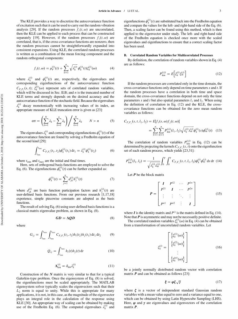
The KLE provides a way to discretize the autocovariance functionof excitation such that it can be used to carry out the random vibrationanalysis [29]. If the random processes fi�t;ω� are uncorrelated,then the KLE can be applied to each process that can be constructedseparately [19]. However, if the random processes fi�t;ω� arecorrelated, that is, if the cross-covariance functions are nonzero, thenthe random processes cannot be straightforwardly expanded intoconsistent expansions. Using KLE, the correlated random processesis written as a combination of the mean forcing component and therandom orthogonal components:

fi�t;ω� � μ�i�F �t� �Xnk�1

�������λ�i�k

qϕ�i�k �t�ξ�i�k �ω� (4)

where λ�i�k and ϕ�i�k �t� are, respectively, the eigenvalues and

corresponding eigenfunctions of the autocovariance function

CFiFi�s; t�; ξ�i�k �ω� represent sets of correlated random variables,

which will be discussed in Sec. II.B; and n is the truncated number ofKLE terms and strongly depends on the desired accuracy and theautocovariance functionof the stochastic field.Because the eigenvalues

λ�i�k decay monotonically with increasing values of its index, an

appropriate measure of KLE truncation error is given as [23]:

err � XN

k�1

λk −Xnk�1

λk

!,XNk�1

λk N > n (5)

The eigenvalues λ�i�k and corresponding eigenfunctionsϕ�i�k �t� of the

autocovariance function are found by solving a Fredholm equation ofthe second kind [29]:Z

tmax

tmin

CFiFi�t1; t2�ϕ�i�

k �t1� dt1 � λ�i�k ϕ�i�k �t2� (6)

where tmin and tmax are the initial and final times.Here, sets of orthogonal basis functions are employed to solve the

Eq. (6). The eigenfunctions ϕ�i�k �t� can be further expanded as:

ϕ�i�k �t� �

Xnj�1

d�i�jk h�i�j �t� (7)

where d�i�jk are basis function participation factors and h�i�j �t� areuser-defined basis functions. From our previous research [1,17,18]experience, simple piecewise constants are adopted as the basisfunctions.The result of solving Eq. (6) using user-defined basis functions is a

classical matrix eigenvalue problem, as shown in Eq. (8).

GD � ΛQD (8)

where

Gij �Z

tmax

tmin

Ztmax

tmin

CFiFi�t1; t2�hi�t2�hj�t1� dt1 dt2 (9)

Qij �Z

tmax

tmin

hi�t�hj�t� dt (10)

Λ�i�km � δkmλ

�i�k (11)

Construction of the N matrix is very similar to that for a typicalGalerkin-type problem. Once the eigensystem of Eq. (8) is solved,the eigenfunctions must be scaled appropriately. The MATLABeigensystem solver typically scales the eigenvectors such that theirL2 norm is equal to unity. While this is appropriate for manyapplications, it is not, in this case, as themagnitude of the eigenvectorplays an integral role in the calculation of the response usingKLE [30]. An appropriate way of scaling can be obtained by makinguse of the Fredholm Eq. (6). The computed eigenvalues λ�i�k and

eigenfunctions ϕ�i�k �t� are substituted back into the Fredholm equation

and compare the values for the left- and right-hand side of the Eq. (6).

Then, a scaling factor can be found using this method, which is then

applied to the eigenvector under study. The left- and right-hand side

of the Fredholm equation is checked once more with the scaled

eigenvalues and eigenfunctions to ensure that a correct scaling factor

has been used.

B. Correlated Random Variables for Multicorrelated Processes

By definition, the correlation of random variables shown in Eq. (4)

are as follows:

P�ij�km � E

hξ�i�k ξ�j�m

i(12)

If the random processes are correlated only in the time domain, the

cross-covariance functions only depend on time parameters s and t. Ifthe random processes have a correlation in both time and space

domain, the cross-covariance functions depend on not only the time

parameters s and t but also spatial parameters l1 and l2. When using

the definition of correlation in Eq. (12) and the KLE, the cross-

covariance functions can be obtained for the zero mean random

variables as follows:

CFiFj�s; t; l1; l2� � E�fi�s;ω�fj�t;ω��

�Xnk�1

Xnm�1

P�ij�km �l1; l2�

��������������λ�i�k λ�j�m

qϕ�i�k �s�ϕ�j�

m �t� (13)

The correlation of random variables P�ij�km in Eq. (12) can be

determinedbyprojecting thekernelsCFiFj�s; t�onto the eigenfunction

set of each random process, which yields [23,31]:

P�ij�km �l1; l2� �

1��������������λ�i�k λ�j�m

q ZT

0

ZT

0

CFiFj�s; t; l1; l2�ϕ�i�

k ϕ�j�m ds dt (14)

Let P be the block matrix

P �

2666664

I P12 · · · P1n

P21 I · · · P2n

..

. ... . .

. ...

Pn1 Pn2 ...

I

3777775 (15)

where I is the identity matrix andPij is the matrix defined in Eq. (14).

Note thatP is asymmetric andmay not be necessarily positive definite.The correlated random variables ξ�i�k �ω� in Eq. (4) can be obtained

from a transformation of uncorrelated random variables. Let

ξ�i�k �

2666666664

nξ�1�k �ω�

onξ�2�k �ω�

o...n

ξ�n�k �ω�o

3777777775

(16)

be a jointly normally distributed random vector with correlation

matrix P and can be obtained as follows [23]:

ξ � φζ���γ

p(17)

where ζ is a vector of independent standard Gaussian random

variables with a mean value equal to zero and a variance equal to one,

which can be obtained by using Latin Hypercube Sampling (LHS).

Here, φ and γ are eigenvalues and eigenvectors of the correlation

matrix P.

Article in Advance / LI ETAL. 3

Dow

nloa

ded

by U

NIV

ER

SIT

Y O

F A

LA

BA

MA

on

Oct

ober

2, 2

018

| http

://ar

c.ai

aa.o

rg |

DO

I: 1

0.25

14/1

.C03

4721

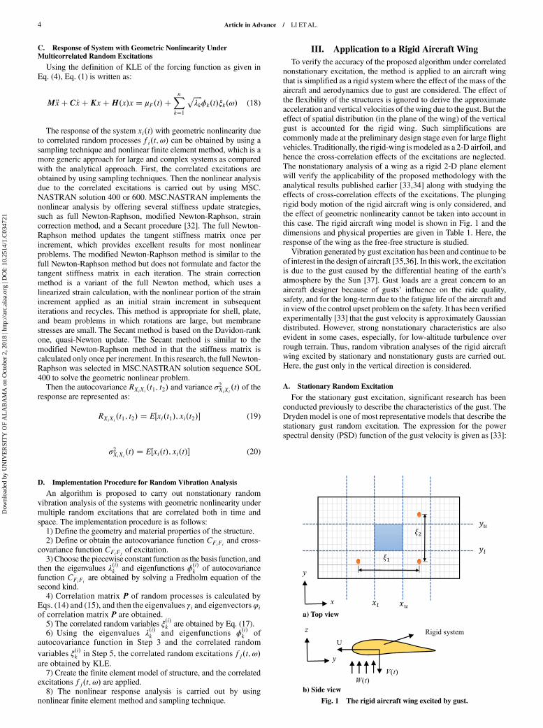
C. Response of System with Geometric Nonlinearity UnderMulticorrelated Random Excitations

Using the definition of KLE of the forcing function as given in

Eq. (4), Eq. (1) is written as:

M �x� C _x� Kx�H�x�x � μF�t� �Xnk�1

�����λk

pϕk�t�ξk�ω� (18)

The response of the system xi�t� with geometric nonlinearity due

to correlated random processes fi�t;ω� can be obtained by using a

sampling technique and nonlinear finite element method, which is a

more generic approach for large and complex systems as compared

with the analytical approach. First, the correlated excitations are

obtained by using sampling techniques. Then the nonlinear analysis

due to the correlated excitations is carried out by using MSC.

NASTRAN solution 400 or 600. MSC.NASTRAN implements the

nonlinear analysis by offering several stiffness update strategies,

such as full Newton-Raphson, modified Newton-Raphson, strain

correction method, and a Secant procedure [32]. The full Newton-

Raphson method updates the tangent stiffness matrix once per

increment, which provides excellent results for most nonlinear

problems. The modified Newton-Raphson method is similar to the

full Newton-Raphson method but does not formulate and factor the

tangent stiffness matrix in each iteration. The strain correction

method is a variant of the full Newton method, which uses a

linearized strain calculation, with the nonlinear portion of the strain

increment applied as an initial strain increment in subsequent

iterations and recycles. This method is appropriate for shell, plate,

and beam problems in which rotations are large, but membrane

stresses are small. The Secant method is based on the Davidon-rank

one, quasi-Newton update. The Secant method is similar to the

modified Newton-Raphson method in that the stiffness matrix is

calculated only once per increment. In this research, the full Newton-

Raphson was selected in MSC.NASTRAN solution sequence SOL

400 to solve the geometric nonlinear problem.Then the autocovariance RXiXi

�t1; t2� and variance σ2XiXi�t� of the

response are represented as:

RXiXi�t1; t2� � E�xi�t1�; xi�t2�� (19)

σ2XiXi�t� � E�xi�t�; xi�t�� (20)

D. Implementation Procedure for Random Vibration Analysis

An algorithm is proposed to carry out nonstationary random

vibration analysis of the systems with geometric nonlinearity under

multiple random excitations that are correlated both in time and

space. The implementation procedure is as follows:1) Define the geometry and material properties of the structure.2) Define or obtain the autocovariance function CFiFi

and cross-covariance function CFiFj

of excitation.3) Choose the piecewise constant function as the basis function, and

then the eigenvalues λ�i�k and eigenfunctions ϕ�i�k of autocovariance

function CFiFiare obtained by solving a Fredholm equation of the

second kind.4) Correlation matrix P of random processes is calculated by

Eqs. (14) and (15), and then the eigenvalues γi and eigenvectors φi

of correlation matrix P are obtained.5) The correlated random variables ξ�i�k are obtained by Eq. (17).6) Using the eigenvalues λ�i�k and eigenfunctions ϕ�i�

k ofautocovariance function in Step 3 and the correlated random

variables ξ�i�k in Step 5, the correlated random excitations fj�t;ω�are obtained by KLE.7) Create the finite element model of structure, and the correlated

excitations fj�t;ω� are applied.8) The nonlinear response analysis is carried out by using

nonlinear finite element method and sampling technique.

III. Application to a Rigid Aircraft Wing

To verify the accuracy of the proposed algorithm under correlated

nonstationary excitation, the method is applied to an aircraft wing

that is simplified as a rigid system where the effect of the mass of the

aircraft and aerodynamics due to gust are considered. The effect of

the flexibility of the structures is ignored to derive the approximate

acceleration and vertical velocities of thewing due to the gust. But the

effect of spatial distribution (in the plane of the wing) of the vertical

gust is accounted for the rigid wing. Such simplifications are

commonly made at the preliminary design stage even for large flight

vehicles. Traditionally, the rigid-wing ismodeled as a 2-D airfoil, and

hence the cross-correlation effects of the excitations are neglected.

The nonstationary analysis of a wing as a rigid 2-D plane element

will verify the applicability of the proposed methodology with the

analytical results published earlier [33,34] along with studying the

effects of cross-correlation effects of the excitations. The plunging

rigid body motion of the rigid aircraft wing is only considered, and

the effect of geometric nonlinearity cannot be taken into account in

this case. The rigid aircraft wing model is shown in Fig. 1 and the

dimensions and physical properties are given in Table 1. Here, the

response of the wing as the free-free structure is studied.

Vibration generated by gust excitation has been and continue to be

of interest in the design of aircraft [35,36]. In this work, the excitation

is due to the gust caused by the differential heating of the earth’s

atmosphere by the Sun [37]. Gust loads are a great concern to an

aircraft designer because of gusts’ influence on the ride quality,

safety, and for the long-term due to the fatigue life of the aircraft and

in view of the control upset problem on the safety. It has been verified

experimentally [33] that the gust velocity is approximately Gaussian

distributed. However, strong nonstationary characteristics are also

evident in some cases, especially, for low-altitude turbulence over

rough terrain. Thus, random vibration analyses of the rigid aircraft

wing excited by stationary and nonstationary gusts are carried out.

Here, the gust only in the vertical direction is considered.

A. Stationary Random Excitation

For the stationary gust excitation, significant research has been

conducted previously to describe the characteristics of the gust. The

Dryden model is one of most representative models that describe the

stationary gust random excitation. The expression for the power

spectral density (PSD) function of the gust velocity is given as [33]:

a) Top view

b) Side view

Fig. 1 The rigid aircraft wing excited by gust.

4 Article in Advance / LI ETAL.

Dow

nloa

ded

by U

NIV

ER

SIT

Y O

F A

LA

BA

MA

on

Oct

ober

2, 2

018

| http

://ar

c.ai

aa.o

rg |

DO

I: 1

0.25

14/1

.C03

4721

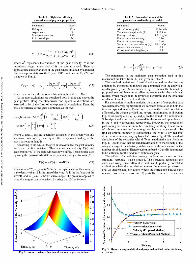
SFiFi�ω� � σ2B

2πU

�1� �3ωB∕U�2�1� �ωB∕U�2�2

�(21)

where σ2 represents the variance of the gust velocity, B is the

turbulence length scale, and U is the aircraft speed. Then an

approximate autocovariance of the gust can be obtained by a transfer

function representation of theDryden PSD function as in Eq. (22) and

is shown in Fig. 2.

CFiFi�t1; t2� � σ2i

�1 −

jt1 − t2j2τi

�exp

�−jt1 − t2j

τi

�(22)

where τi represents the autocorrelation length, and τi � B∕U.As the gust excitations are correlated both in time and space, the

gust profiles along the streamwise and spanwise directions are

assumed to be of the form of an exponential correlation. Then, the

cross-covariance of the gust is obtained as follows:

CFiFj�ζ1; ζ2; t1; t2� �

σ2iτij

�1 −

jt1 − t2j2τij

�exp

�−jt1 − t2j

τij

�

× exp

�−γ1

���� ζ1U�����exp

�−γ2

���� ζ2U�����

(23)

where ζ1 and ζ2 are the separation distances in the streamwise and

spanwise directions, γ1 and γ2 are the decay rates, and τij is the

cross-correlation length.According to the KLE of the gust autocovariance, the gust velocity

W�t� can be first obtained. Then the vertical velocity V�t� and

acceleration _V�t� of the rigidwing as shown in Fig. 1 can be calculatedby using the quasi-steady state aerodynamics theory as follows [37]:

_V�t� � aV�t� � −aW�t� (24)

wherea � ρUS�dCL∕dα�∕2M is themass parameter of the aircraft, ρis the density of air, S is the area of the wing,M is the half mass of the

aircraft, and dCL∕dα is the lift curve slope. The pressure applied to

wing due to gust can be obtained by using Eq. (24) as follows:

P�t� � 1

2ρU

dCL

dα�W�t� � V�t�� (25)

The parameters of the stationary gust excitation used in thismanuscript are taken from [37] and given in Table 2.The standard deviations of vertical velocity and acceleration are

obtained by the proposed method and compared with the analyticalresults given by Lee [34] as shown in Fig. 3. The results obtained byproposed method have an excellent agreement with the analyticalresults, which means that the proposed algorithm and the obtainedresults are feasible, correct, and valid.For the random vibration analysis, the amount of computing data

would become very significant if we consider correlation in both thetime and space domains. Therefore, to capture the spatial correlationefficiently, the wing is divided into several subdomains, as shown inFig. 1; for example, xl, xu, yl, and yu are the bounds of a subdomain.Subscripts l and u on x and y are used for the lower and upper boundsin the x and y directions, respectively. However, the process ofpartitioning the domain cannot be completely arbitrary. The divisionof subdomains must be fine enough to obtain accurate results. Tofind an optimal number of subdomains, the wing is divided intodifferent subdomains, varying from 1 × 1 to 6 × 3 grid. The standarddeviations of the velocities with different subdomains are shown inFig. 4. Results show that the standard deviations of the velocity of thewing converge to a relatively stable value with an increase in thenumberof subdomains.Therefore, the number6 × 3grid isdeterminedto be sufficient for the random vibration analysis.The effect of correlation among random excitations on the

structural response is also studied. The structural responses arecalculated using three different excitations: 1) perfectly correlatedexcitations where the correlation between the random processes isone, 2) uncorrelated excitations where the correlation between therandom processes is zero, and 3) partially correlated excitations

Fig. 2 Autocovariance function of stationary gust excitation.

Table 1 Rigid aircraft wingdimensions and physical properties

Parameters Values

Full span 50 mAspect ratio 5Mass parameter (a) 1.12Lift curve slope 2π

Table 2 Numerical values of theparameters used in the gust model

Parameters Values

Aircraft velocity (U) 60.96 m∕sTurbulence length scale (B) 152.4 mDensity of air (ρ) 1.21 kg∕m3

Decay rate, streamwise (γ1) 0.16Decay rate, spanwise (γ2) 0.46Variance of the gust velocity (σ2i ) 0.81 m2∕s2Autocorrelation length (τi) 2.5Cross-correlation length (τii) 2.5

0 1 2 3 40

0.3

0.6

0.9

1.2

Time (s)

Stan

dard

Dev

iati

on o

f th

e ve

loci

ty a

nd a

ccel

erat

ion

Velocity (Analytical)Acceleration (Analytical)Velocity (Proposed Method)Acceleration (Proposed Method)

Fig. 3 Results using analytical and proposed method under stationaryexcitation.

Article in Advance / LI ETAL. 5

Dow

nloa

ded

by U

NIV

ER

SIT

Y O

F A

LA

BA

MA

on

Oct

ober

2, 2

018

| http

://ar

c.ai

aa.o

rg |

DO

I: 1

0.25

14/1

.C03

4721

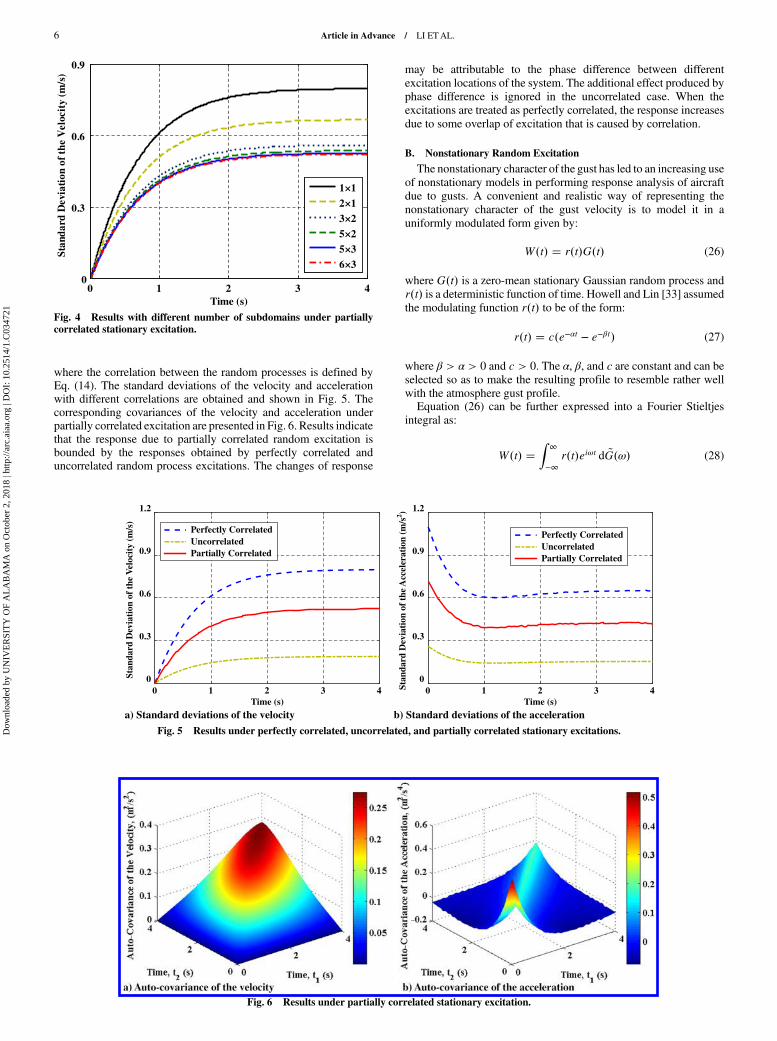
where the correlation between the random processes is defined byEq. (14). The standard deviations of the velocity and accelerationwith different correlations are obtained and shown in Fig. 5. Thecorresponding covariances of the velocity and acceleration underpartially correlated excitation are presented in Fig. 6. Results indicatethat the response due to partially correlated random excitation isbounded by the responses obtained by perfectly correlated anduncorrelated random process excitations. The changes of response

may be attributable to the phase difference between different

excitation locations of the system. The additional effect produced by

phase difference is ignored in the uncorrelated case. When the

excitations are treated as perfectly correlated, the response increases

due to some overlap of excitation that is caused by correlation.

B. Nonstationary Random Excitation

The nonstationary character of the gust has led to an increasing use

of nonstationary models in performing response analysis of aircraft

due to gusts. A convenient and realistic way of representing the

nonstationary character of the gust velocity is to model it in a

uniformly modulated form given by:

W�t� � r�t�G�t� (26)

where G�t� is a zero-mean stationary Gaussian random process and

r�t� is a deterministic function of time. Howell and Lin [33] assumed

the modulating function r�t� to be of the form:

r�t� � c�e−αt − e−βt� (27)

where β > α > 0 and c > 0. The α, β, and c are constant and can beselected so as to make the resulting profile to resemble rather well

with the atmosphere gust profile.Equation (26) can be further expressed into a Fourier Stieltjes

integral as:

W�t� �Z

∞

−∞r�t�eiωt d ~G�ω� (28)

0 1 2 3 40

0.3

0.6

0.9

Time (s)

Stan

dard

Dev

iati

on o

f the

Vel

ocit

y (m

/s)

1×12×13×25×25×36×3

Fig. 4 Results with different number of subdomains under partiallycorrelated stationary excitation.

Fig. 6 Results under partially correlated stationary excitation.

a) Standard deviations of the velocity b) Standard deviations of the accelerationTime (s)

0 1 2 3 4

Stan

dard

Dev

iati

on o

f th

e V

eloc

ity

(m/s

)

0

0.3

0.6

0.9

1.2

Perfectly CorrelatedUncorrelatedPartially Correlated

Time (s)0 1 2 3 4St

anda

rd D

evia

tion

of

the

Acc

eler

atio

n (m

/s2 )

0

0.3

0.6

0.9

1.2

Perfectly CorrelatedUncorrelatedPartially Correlated

Fig. 5 Results under perfectly correlated, uncorrelated, and partially correlated stationary excitations.

6 Article in Advance / LI ETAL.

Dow

nloa

ded

by U

NIV

ER

SIT

Y O

F A

LA

BA

MA

on

Oct

ober

2, 2

018

| http

://ar

c.ai

aa.o

rg |

DO

I: 1

0.25

14/1

.C03

4721

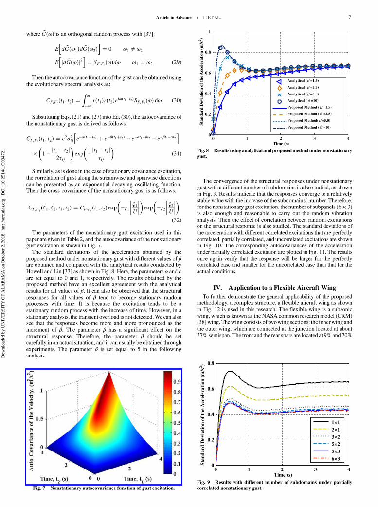
where ~G�ω� is an orthogonal random process with [37]:

Ehd ~G�ω1�d ~G�ω2�

i� 0 ω1 ≠ ω2

Ehjd ~G�ω�j2

i� SFiFi

�ω�dω ω1 � ω2 (29)

Then the autocovariance function of the gust can be obtained usingthe evolutionary spectral analysis as:

CFiFi�t1; t2� �

Z∞

−∞r�t1�r�t2�eiω�t1−t2�SFiFi

�ω� dω (30)

Substituting Eqs. (21) and (27) into Eq. (30), the autocovariance ofthe nonstationary gust is derived as follows:

CFiFi�t1; t2� � c2σ2ij

he−α�t1�t2� � e−β�t1�t2� − e−αt1−βt2 − e−βt1−αt2

i×�1 −

jt1 − t2j2τij

�exp

�−jt1 − t2j

τij

�(31)

Similarly, as is done in the case of stationary covariance excitation,the correlation of gust along the streamwise and spanwise directionscan be presented as an exponential decaying oscillating function.Then the cross-covariance of the nonstationary gust is as follows:

CFiFj�ζ1; ζ2; t1; t2� � CFiFi

�t1; t2� exp�−γ1

���� ζ1U�����exp

�−γ2

���� ζ2U�����

(32)

The parameters of the nonstationary gust excitation used in thispaper are given in Table 2, and the autocovariance of the nonstationarygust excitation is shown in Fig. 7.The standard deviations of the acceleration obtained by the

proposed method under nonstationary gust with different values of βare obtained and compared with the analytical results conducted byHowell and Lin [33] as shown in Fig. 8. Here, the parameters α and care set equal to 0 and 1, respectively. The results obtained by theproposed method have an excellent agreement with the analyticalresults for all values of β. It can also be observed that the structuralresponses for all values of β tend to become stationary randomprocesses with time. It is because the excitation tends to be astationary random process with the increase of time. However, in astationary analysis, the transient overload is not detected.We can alsosee that the responses become more and more pronounced as theincrement of β. The parameter β has a significant effect on thestructural response. Therefore, the parameter β should be setcarefully in an actual situation, and it can usually be obtained throughexperiments. The parameter β is set equal to 5 in the followinganalysis.

The convergence of the structural responses under nonstationarygust with a different number of subdomains is also studied, as shownin Fig. 9. Results indicate that the responses converge to a relativelystable valuewith the increase of the subdomains’ number. Therefore,for the nonstationary gust excitation, the number of subpanels (6 × 3)is also enough and reasonable to carry out the random vibrationanalysis. Then the effect of correlation between random excitationson the structural response is also studied. The standard deviations ofthe acceleration with different correlated excitations that are perfectlycorrelated, partially correlated, and uncorrelated excitations are shownin Fig. 10. The corresponding autocovariances of the accelerationunder partially correlated excitation are plotted in Fig. 11. The resultsonce again verify that the response will be larger for the perfectlycorrelated case and smaller for the uncorrelated case than that for theactual conditions.

IV. Application to a Flexible Aircraft Wing

To further demonstrate the general applicability of the proposedmethodology, a complex structure, a flexible aircraft wing as shownin Fig. 12 is used in this research. The flexible wing is a subsonicwing, which is known as the NASA common research model (CRM)[38]wing. Thewing consists of twowing sections: the innerwing andthe outer wing, which are connected at the junction located at about37% semispan. The front and the rear spars are located at 9%and 70%

Fig. 7 Nonstationary autocovariance function of gust excitation.

Time (s)0 1 2 3 4

Stan

dard

Dev

iati

on o

f th

e A

ccel

erat

ion

(m/s

2 )

0

0.2

0.4

0.6

0.8

1

Analytical ( =1.5)

Analytical ( =2.5)

Analytical ( =5.0)

Analytical ( =10)

Proposed Method ( =1.5)

Proposed Method ( =2.5)

Proposed Method( =5.0)

Proposed Method ( =10)

Fig. 8 Resultsusinganalytical andproposedmethodundernonstationarygust.

0 1 2 3 40

0.2

0.4

0.6

0.8

Time (s)

Stan

dard

Dev

iati

on o

f the

Acc

eler

atio

n (m

/s2 )

1×12×13×25×25×36×3

Fig. 9 Results with different number of subdomains under partiallycorrelated nonstationary gust.

Article in Advance / LI ETAL. 7

Dow

nloa

ded

by U

NIV

ER

SIT

Y O

F A

LA

BA

MA

on

Oct

ober

2, 2

018

| http

://ar

c.ai

aa.o

rg |

DO

I: 1

0.25

14/1

.C03

4721

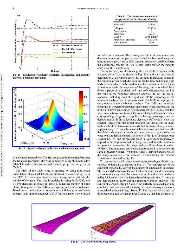
of the chord, respectively. The ribs are placed in the region between

the front and rear spars. The wing is modeled using aluminum alloy

2024-T3, and its dimensions and material properties are given in

Table 3.

The FEM of the CRM wing is modeled by using four-noded

quadrilateral elements (CQUAD4 inNastran), as shown in Fig. 12. In

the FEM, it is important to study the convergence to estimate the

number of elements. The wing is modeled by using 4142, 9540, and

31,140 elements, as shown in Table 4. When the number of finite

elements is greater than 9540, converged results can be obtained.

Based on a combination of computational efficiency and sufficient

accuracy, this optimum number 9540 of finite elements is determined

for subsequent analysis. The convergence of the structural responsedue to a number of samples is also studied for both stationary andnonstationary gust. A set of 1000 samples of random variables wherethe confidence reaches 98.11% is also sufficient for the randomanalysis of the flexible wing.During the analysis of this wing, the root of the wing is usually

assumed to be fixed as shown in Fig. 13a, and thus only elasticdeformation of the wing is taken into account. In an actual situation,the response of wing includes both the elastic deformation and rigidbody motion, which can be used for comfort evaluation. In the linearvibration analysis, the response of the wing can be obtained by alinear superposition of elastic and rigid body deformations, but it isnot valid in the nonlinear vibration analysis. To get the overallresponse, including both the rigid and elastic responses in thenonlinear analysis, the large mass method (LMM) is employed tocarry out the random vibration analysis. The LMM is a modelingtechnique inwhich the user places an element with a largemass at thepoints of known acceleration or displacement [39,40]. In effect, thislargemass acts as a constraint at the connected point/location. Then, acorrespondingly large force is applied to the largemass to produce thedesired motion. If the added mass element is sufficiently heavy, thereaction forces from the actual structure will not affect the inputmotions. MSC software recommends that the value of large mass isapproximately 106 times themass of the entire structure. In this work,the LMM is simulated by attaching a hugemass that is attached to thewing by using RBE2 elements, as shown in Fig. 13b. The large forcegiven in Eq. (24) and the pressure given in Eq. (25) are, respectively,applied to the large mass and the wing skin, and then the nonlinearresponse can be obtained by using nonlinear finite element method(NFEM). The stationary and nonstationary gusts in this section aresame as given in Sec. III. Twopoints,A andB, at the tip and the root ofthe wing, respectively, are selected for monitoring the randomvibrations, as marked in Fig. 13.To capture the spatial correlation of a gust, the wing is divided into

several subdomains, as shown in Fig. 14. The convergence of thestructural response by varying the number of subdomains is studied.The standard deviations of the acceleration at point A under stationaryand nonstationary gustswith various number of subdomains are showninFig. 15. Results show that the number of subpanels (6 × 4) is enoughand reasonable to carry out the random vibration analysis. Thestructural responses at point A due to the perfectly correlated, partiallycorrelated, and uncorrelated stationary and nonstationary excitationsare obtained as shown in Figs. 16 and 17. The standard deviation at thetip is becoming less oscillatory after 2 s, and the standard deviation of

Fig. 11 Results under partially correlated nonstationary gust.

Time (s)0 1 2 3 4

Stan

dard

Dev

iati

on o

f th

e A

ccel

erat

ion

(m/s

2 )

0

0.2

0.4

0.6

0.8

Perfectly Correlated

Partially Correlated

Uncorrelated

Fig. 10 Results under perfectly correlated, uncorrelated, and partiallycorrelated nonstationary gusts.

Table 3 The dimensions and materialproperties of the flexible aircraft wing

Parameters Values

Full span 58.75 mAspect ratio 9Taper ratio 0.275Density 2768 kg∕m3

Modulus of elasticity 73.09 GPaPoisson ratio 0.33

Fig. 12 The flexible aircraft wing model.

8 Article in Advance / LI ETAL.

Dow

nloa

ded

by U

NIV

ER

SIT

Y O

F A

LA

BA

MA

on

Oct

ober

2, 2

018

| http

://ar

c.ai

aa.o

rg |

DO

I: 1

0.25

14/1

.C03

4721

displacement is becoming almost linearly increasing due to themodeling of the wing as a free-free structure will produce a rigidmotion. The same conclusion as obtained in Sec. III is confirmed againthat the structural responses due to correlated random processes arebounded by the response achieved by both perfectly correlated anduncorrelated random excitations.Theoretically, themore samples of randomvariables are used in the

sampling technique, the more accurate results will be obtained. Here,

LHS [41] is used to generate samples. However, the computationalcost will be too high if one uses a large number of samples to carry outthe random vibration analysis, especially for the case of nonlinearvibration. It is necessary to obtain an optimum number of samplesbased on computational efficiency and sufficient accuracy. To findthis optimal number, the stationary and nonstationary nonlinearrandomvibration analyses are carried out by using 200, 400, 600, 800,and 1000 samples of random variables. The confidence levels withdifferent values of sampling numbers are shown in Table 5, where theconfidence interval is 95%. Results demonstrate that the confidenceincreases with an increase in the number of samples, and it reaches98.11% when 1000 samples are used. Thus, a set of 1000 samples ofrandom variables is sufficient for this problem.To study the effect of geometric nonlinearity on the structural

response, the standard deviations of displacement and acceleration atpoint A obtained using nonlinear analysis due to LMM and fixedboundary conditions are calculated and comparedwith the linear caseresults, as shown in Figs. 18 and 19, respectively. Results showthat the geometric nonlinear effect has a hardening effect on thiswing’s response and results in a less oscillatory response amplitudecompared with the linear case. Moreover, the geometric nonlineareffect results in stiffening of the aircraft wing, which decreases thewing’s response. This is because a large out-of-plane deformation ofthe wing results in in-plane stretching, which in turn leads to ahardening of thewing. However, it is worth noticing that the effect ofnonlinear stiffnessmatrix is not always stiffening. It may also have an

Table 4 The first 10 natural frequencies of the flexible aircraft wing (Hz)

Number of elements 1 2 3 4 5 6 7 8 9 10

4,142 1.54 5.51 8.91 11.05 11.23 12.60 12.85 13.09 13.65 13.979,540 1.27 4.90 8.32 10.36 10.58 11.05 11.44 11.70 12.06 12.1831,140 1.26 4.87 8.27 10.08 10.31 10.85 11.18 11.56 11.92 12.07

Fig. 13 The fixed and LMM boundary condition of the flexible aircraft wing.

Fig. 14 Subdomains to capture the correlation on an aircraft wing.

a) Results under stationary gust b) Results under non-stationary gust

0 1 2 3 40

25

50

75

100

Time (s)

Sta

nd

ard

Dev

iati

on o

f th

e A

ccel

erat

ion

(m

/s2 )

Sta

nd

ard

Dev

iati

on o

f th

e A

ccel

erat

ion

(m

/s2 )

1×3

2×43×5

4×6

0 1 2 3 40

12

24

36

48

Time (s)

1×3

2×43×5

4×6

Fig. 15 Results with different number of subdomains under stationary and nonstationary gust.

Article in Advance / LI ETAL. 9

Dow

nloa

ded

by U

NIV

ER

SIT

Y O

F A

LA

BA

MA

on

Oct

ober

2, 2

018

| http

://ar

c.ai

aa.o

rg |

DO

I: 1

0.25

14/1

.C03

4721

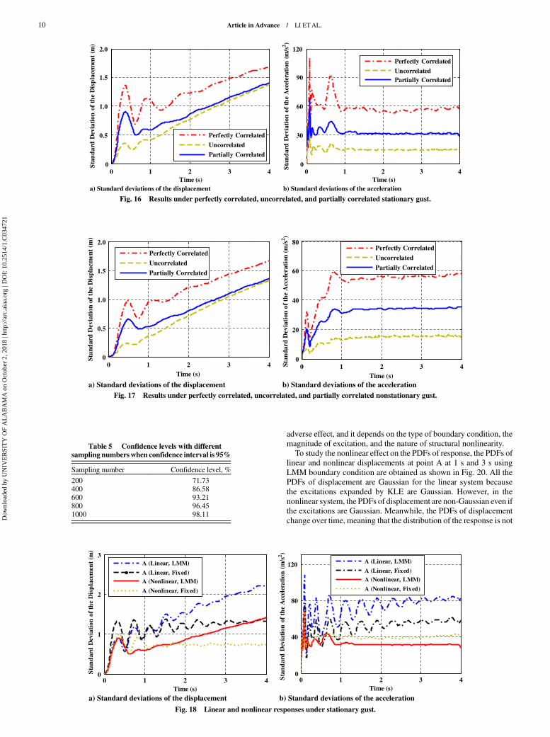
adverse effect, and it depends on the type of boundary condition, the

magnitude of excitation, and the nature of structural nonlinearity.

To study the nonlinear effect on the PDFs of response, the PDFs of

linear and nonlinear displacements at point A at 1 s and 3 s using

LMM boundary condition are obtained as shown in Fig. 20. All the

PDFs of displacement are Gaussian for the linear system because

the excitations expanded by KLE are Gaussian. However, in the

nonlinear system, the PDFs of displacement are non-Gaussian even if

the excitations are Gaussian. Meanwhile, the PDFs of displacement

change over time, meaning that the distribution of the response is not

a) Standard deviations of the displacement b) Standard deviations of the acceleration

0 1 2 3 40

0.5

1.0

1.5

2.0

Time (s)

Sta

nd

ard

Dev

iati

on o

f th

e D

isp

lace

men

t (m

)

Perfectly Correlated

Uncorrelated

Partially Correlated

0 1 2 3 40

30

60

90

120

Time (s)

Sta

nd

ard

Dev

iati

on o

f th

e A

ccel

erat

ion

(m

/s2 )

Perfectly Correlated

UncorrelatedPartially Correlated

Fig. 16 Results under perfectly correlated, uncorrelated, and partially correlated stationary gust.

a) Standard deviations of the displacement b) Standard deviations of the acceleration

0 1 2 3 40

0.5

1.0

1.5

2.0

Time (s)

Stan

dard

Dev

iati

on o

f th

e D

ispl

acm

ent

(m)

Perfectly Correlated

Uncorrelated

Partially Correlated

0 1 2 3 40

20

40

60

80

Time (s)

Stan

dard

Dev

iati

on o

f th

e A

ccel

erat

ion

(m/s

2 )

Perfectly Correlated

Uncorrelated

Partially Correlated

Fig. 17 Results under perfectly correlated, uncorrelated, and partially correlated nonstationary gust.

Table 5 Confidence levels with differentsampling numberswhen confidence interval is 95%

Sampling number Confidence level, %

200 71.73400 86.58600 93.21800 96.451000 98.11

a) Standard deviations of the displacement b) Standard deviations of the acceleration

0 1 2 3 40

1

2

3

Time (s)

Sta

nd

ard

Dev

iati

on o

f th

e D

isp

lace

men

t (m

)

A (Linear, LMM)

A (Linear, Fixed)A (Nonlinear, LMM)

A (Nonlinear, Fixed)

0 1 2 3 40

40

80

120

Time (s)

Sta

nd

ard

Dev

iati

on o

f th

e A

ccel

erat

ion

(m

/s2 )

A (Linear, LMM)

A (Linear, Fixed)A (Nonlinear, LMM)

A (Nonlinear, Fixed)

Fig. 18 Linear and nonlinear responses under stationary gust.

10 Article in Advance / LI ETAL.

Dow

nloa

ded

by U

NIV

ER

SIT

Y O

F A

LA

BA

MA

on

Oct

ober

2, 2

018

| http

://ar

c.ai

aa.o

rg |

DO

I: 1

0.25

14/1

.C03

4721

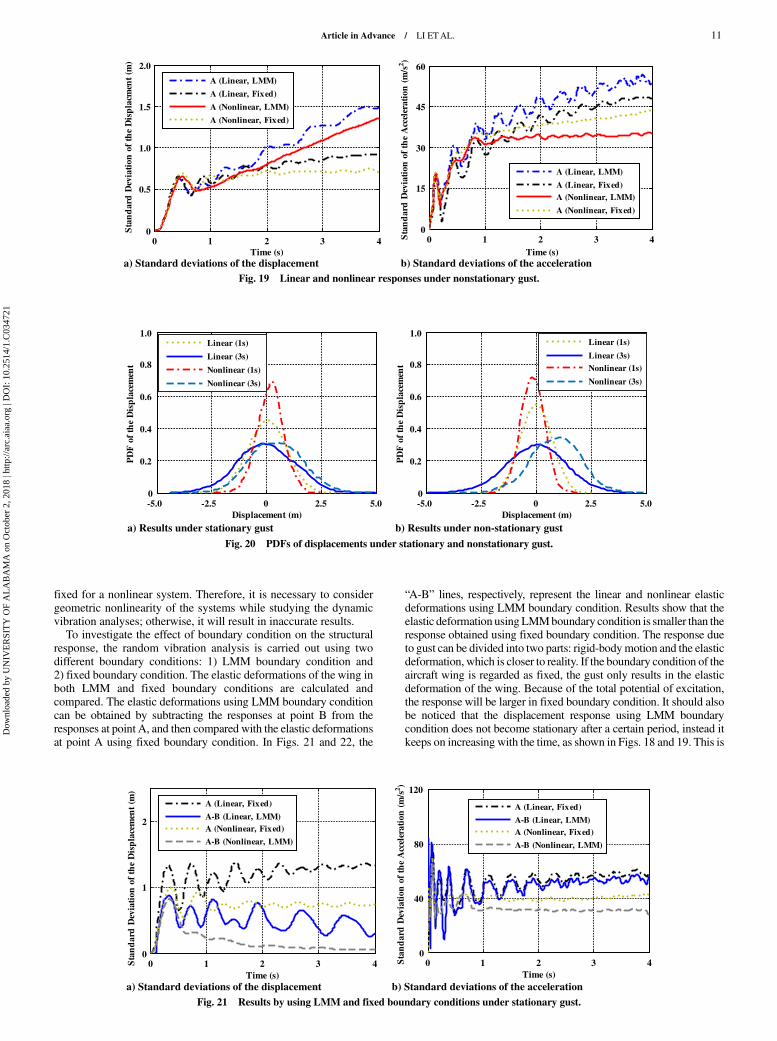
fixed for a nonlinear system. Therefore, it is necessary to considergeometric nonlinearity of the systems while studying the dynamicvibration analyses; otherwise, it will result in inaccurate results.To investigate the effect of boundary condition on the structural

response, the random vibration analysis is carried out using twodifferent boundary conditions: 1) LMM boundary condition and2) fixed boundary condition. The elastic deformations of the wing inboth LMM and fixed boundary conditions are calculated andcompared. The elastic deformations using LMM boundary conditioncan be obtained by subtracting the responses at point B from theresponses at point A, and then compared with the elastic deformationsat point A using fixed boundary condition. In Figs. 21 and 22, the

“A-B” lines, respectively, represent the linear and nonlinear elasticdeformations using LMM boundary condition. Results show that theelastic deformation usingLMMboundary condition is smaller than theresponse obtained using fixed boundary condition. The response dueto gust can be divided into two parts: rigid-bodymotion and the elasticdeformation, which is closer to reality. If the boundary condition of theaircraft wing is regarded as fixed, the gust only results in the elasticdeformation of the wing. Because of the total potential of excitation,the response will be larger in fixed boundary condition. It should alsobe noticed that the displacement response using LMM boundarycondition does not become stationary after a certain period, instead itkeeps on increasing with the time, as shown in Figs. 18 and 19. This is

a) Standard deviations of the displacement b) Standard deviations of the acceleration

0 1 2 3 40

0.5

1.0

1.5

2.0

Time (s)

Sta

nd

ard

Dev

iati

on o

f th

e D

isp

lacm

ent

(m)

A (Linear, LMM)

A (Linear, Fixed)

A (Nonlinear, LMM)

A (Nonlinear, Fixed)

0 1 2 3 40

15

30

45

60

Time (s)

Sta

nd

ard

Dev

iati

on o

f th

e A

ccel

erat

ion

(m

/s2 )

A (Linear, LMM)

A (Linear, Fixed)A (Nonlinear, LMM)

A (Nonlinear, Fixed)

Fig. 19 Linear and nonlinear responses under nonstationary gust.

a) Results under stationary gust b) Results under non-stationary gust

-5.0 -2.5 0 2.5 5.00

0.2

0.4

0.6

0.8

1.0

Displacement (m)

PD

F o

f th

e D

isp

lace

men

t

Linear (1s)

Linear (3s)

Nonlinear (1s)

Nonlinear (3s)

-5.0 -2.5 0 2.5 5.00

0.2

0.4

0.6

0.8

1.0

Displacement (m)

PD

F o

f th

e D

isp

lace

men

t

Linear (1s)

Linear (3s)

Nonlinear (1s)

Nonlinear (3s)

Fig. 20 PDFs of displacements under stationary and nonstationary gust.

a) Standard deviations of the displacement b) Standard deviations of the acceleration

0 1 2 3 40

1

2

Time (s)

Sta

nd

ard

Dev

iati

on o

f th

e D

isp

lace

men

t (m

)

A (Linear, Fixed)

A-B (Linear, LMM)A (Nonlinear, Fixed)

A-B (Nonlinear, LMM)

0 1 2 3 40

40

80

120

Time (s)

Sta

nd

ard

Dev

iati

on o

f th

e A

ccel

erat

ion

(m

/s2 )

A (Linear, Fixed)

A-B (Linear, LMM)A (Nonlinear, Fixed)

A-B (Nonlinear, LMM)

Fig. 21 Results by using LMM and fixed boundary conditions under stationary gust.

Article in Advance / LI ETAL. 11

Dow

nloa

ded

by U

NIV

ER

SIT

Y O

F A

LA

BA

MA

on

Oct

ober

2, 2

018

| http

://ar

c.ai

aa.o

rg |

DO

I: 1

0.25

14/1

.C03

4721

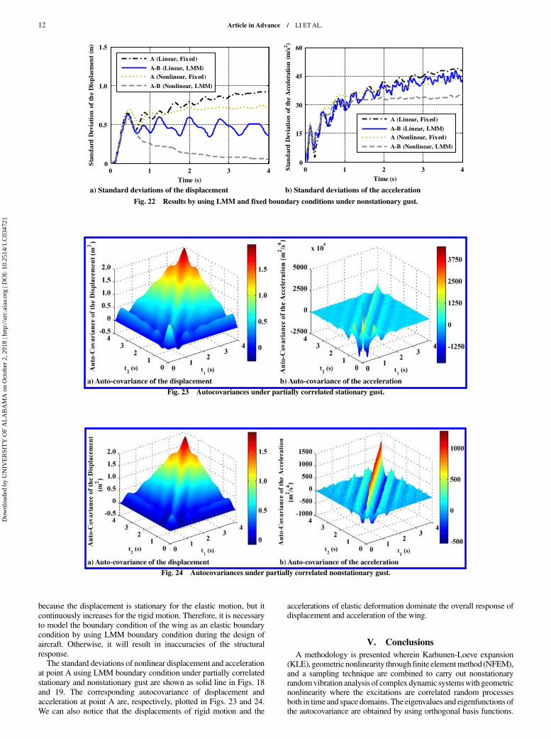
because the displacement is stationary for the elastic motion, but itcontinuously increases for the rigid motion. Therefore, it is necessaryto model the boundary condition of the wing as an elastic boundarycondition by using LMM boundary condition during the design ofaircraft. Otherwise, it will result in inaccuracies of the structuralresponse.The standard deviations of nonlinear displacement and acceleration

at point A using LMM boundary condition under partially correlatedstationary and nonstationary gust are shown as solid line in Figs. 18and 19. The corresponding autocovariance of displacement andacceleration at point A are, respectively, plotted in Figs. 23 and 24.We can also notice that the displacements of rigid motion and the

accelerations of elastic deformation dominate the overall response ofdisplacement and acceleration of the wing.

V. Conclusions

A methodology is presented wherein Karhunen-Loeve expansion(KLE), geometric nonlinearity through finite elementmethod (NFEM),and a sampling technique are combined to carry out nonstationaryrandomvibration analysis of complex dynamic systemswithgeometricnonlinearity where the excitations are correlated random processesboth in time and space domains. The eigenvalues and eigenfunctions ofthe autocovariance are obtained by using orthogonal basis functions.

a) Standard deviations of the displacement b) Standard deviations of the acceleration

0 1 2 3 40

0.5

1.0

1.5

Time (s)

Sta

nd

ard

Dev

iati

on o

f th

e D

isp

lacm

ent

(m)

A (Linear, Fixed)

A-B (Linear, LMM)A (Nonlinear, Fixed)

A-B (Nonlinear, LMM)

0 1 2 3 40

15

30

45

60

Time (s)

Sta

nd

ard

Dev

iati

on o

f th

e A

ccel

erat

ion

(m

/s2 )

A (Linear, Fixed)

A-B (Linear, LMM)A (Nonlinear, Fixed)

A-B (Nonlinear, LMM)

Fig. 22 Results by using LMM and fixed boundary conditions under nonstationary gust.

Fig. 23 Autocovariances under partially correlated stationary gust.

Fig. 24 Autocovariances under partially correlated nonstationary gust.

12 Article in Advance / LI ETAL.

Dow

nloa

ded

by U

NIV

ER

SIT

Y O

F A

LA

BA

MA

on

Oct

ober

2, 2

018

| http

://ar

c.ai

aa.o

rg |

DO

I: 1

0.25

14/1

.C03

4721

The KLE for correlated random excitations relies on expansions interms of the correlated sets of random variables reflecting the cross-covariance of the random excitations. The autocovariance functions ofrandom excitations are discretized into a series of correlated forces thatare applied as excitations, and the structural responses are obtained byusing NFEM and a sampling technique.The application of the proposed algorithm is first carried out to a

rigid aircraft wing under stationary and nonstationary correlatedgusts. To capture the spatial correlation efficiently, thewing is dividedinto several subdomains, and then the number of subdomains isdetermined by a convergence study. The response due to correlatedrandom processes is bounded by the response obtained by perfectlycorrelated and uncorrelated random process excitations. Second, thealgorithm is applied to a flexible aircraftwing. The effects of geometricnonlinearity on the magnitude and distribution of structural responseare carried out. Results show that the geometric nonlinearity hasa hardening effect on the wing response, which suppresses theoscillatory response, and changes the distribution of the responses intonon-Gaussian although the excitations are Gaussian. Next, twodifferent types of the boundary conditions of the wing are studied andresults compared: 1) fixed boundary condition and 2) LMM boundarycondition. The response due to LMM boundary condition, which iscloser to reality, is smaller than the response obtained using fixedboundary condition. The proposed methodology can be applied to theanalysis of any complex structures and any random excitations. Thisstudy will be helpful for the design of aircraft.

Acknowledgments

The work described in this paper was supported by the JiangsuNatural Science Foundation (BK20170656, BK20170022) andthe National Natural Science Foundation of China (11572086,11402052).

References

[1] Mulani, S. B., Kapania, R. K., and Scott, K. M. L., “Generalized LinearRandom Vibration Analysis Using Autocovariance Orthogonal Decom-position,” AIAA Journal, Vol. 48, No. 8, 2010, pp. 1652–1661.doi:10.2514/1.J050033

[2] Hoblit, F. M., Gust Loads on Aircraft: Concepts and Applications,AIAA Education Series, AIAA, Reston, VA, 1988, Chap. 1.

[3] Ghanem, R., and Spanos, P. D., “A Stochastic Galerkin Expansion forNonlinear Random Vibration Analysis,” Probabilistic Engineering

Mechanics, Vol. 8, Nos. 3–4, 1993, pp. 255–264.doi:10.1016/0266-8920(93)90019-R

[4] Roberts, J. B., and Spanos, P. D., Random Vibration and Statistical

Linearization, Wiley, New York, 2003, Chap. 7.[5] Benaroya, H., and Han, S. M., Probability Models in Engineering and

Science, CRC Press, Boca Raton, FL, 2005, Chap. 6.[6] Spanos, P. D., Tezcan, J., and Tratskas, P., “Stochastic Processes

Evolutionary Spectrum Estimation via Harmonic Wavelets,” ComputerMethods in Applied Mechanics and Engineering, Vol. 194, No. 12,2005, pp. 1367–1383.doi:10.1016/j.cma.2004.06.039

[7] Stefanou, G., “The Stochastic Finite ElementMethod: Past, Present andFuture,” Computer Methods in Applied Mechanics and Engineering,Vol. 198, No. 9, 2009, pp. 1031–1051.doi:10.1016/j.cma.2008.11.007

[8] Wirshing, P. H., Paez, T. L., and Keith, O., Random Vibrations: Theory

and Practice, Dover, New York, 1995, Chap. 5.[9] Newland, D. E., An Introduction to Random Vibrations, Spectral &

Wavelet Analysis, Courier Corp., New York, 2012, Chap. 5.[10] Pradlwarter, H. J., Schueller, G. I., and Schenk, C.A., “AComputational

Procedure to Estimate the Stochastic Dynamic Response of LargeNon-Linear FE-Models,”ComputerMethods in AppliedMechanics and

Engineering, Vol. 192, No. 7, 2003, pp. 777–801.doi:10.1016/S0045-7825(02)00595-9

[11] Choi, S. K., Grandhi, R. V., and Canfield, R. A., Reliability-BasedStructural Design, Springer–Verlag, London, 2007, Chap. 2.

[12] Pranesh, S., and Ghosh, D., “Faster Computation of the Karhunen–Loève ExpansionUsing Its Domain Independence Property,”ComputerMethods in AppliedMechanics and Engineering, Vol. 285, No. 3, 2015,pp. 125–145.doi:10.1016/j.cma.2014.10.053

[13] Sakamoto, S., and Ghanem, R., “Polynomial Chaos Decompositionfor the Simulation of Non-Gaussian Nonstationary StochasticProcesses,” Journal of Engineering Mechanics, Vol. 128, No. 2,2002, pp. 190–201.

doi:10.1061/(ASCE)0733-9399(2002)128:2(190)[14] Phoon, K. K., Huang, S. P., and Quek, S. T., “Implementation of

Karhunen–Loeve Expansion for Simulation Using a Wavelet-GalerkinScheme,” Probabilistic Engineering Mechanics, Vol. 17, No. 3, 2002,

pp. 293–303.doi:10.1016/S0266-8920(02)00013-9

[15] Mulani, S. B., Kapania, R. K., and Walters, R. W., “Karhunen-LoeveExpansion of Non-Gaussian Random Process,” 48th AIAA/ASME/

ASCE/AHS/ASC Structures, Structural Dynamics, and Materials

Conference, AIAA Paper 2007-1943, April 2007.[16] Phoon,K.K.,Huang,H.W., andQuek,S.T., “SimulationofStronglyNon-

Gaussian Processes Using Karhunen–Loève Expansion,” Probabilistic

Engineering Mechanics, Vol. 20, No. 2, 2005, pp. 188–198.doi:10.1016/j.probengmech.2005.05.007

[17] Li, Y.,Mulani, S. B., Scott, K.M. L., Kapania, R.K.,Wu, S., and Fei, Q.,“Non-Stationary Random Vibration Analysis of Multi Degree Systems

Using Auto-Covariance Orthogonal Decomposition,” Journal of Soundand Vibration, Vol. 372, No. 23, 2016, pp. 147–167.doi:10.1016/j.jsv.2016.02.018

[18] Scott, K. M. L., “Practical Analysis Tools for Structures Subjected toFlow-Induced and Non-Stationary Random Load,” Ph.D. Dissertation,Aerospace andOcean EngineeringDept., Virginia Polytechnic Inst. andState Univ., Blacksburg, VA, 2011.

[19] Huang, S. P., Quek, S. T., and Phoon, K. K., “Convergence Study of theTruncated Karhunen-Loeve Expansion for Simulation of StochasticProcesses,” International Journal forNumericalMethods inEngineering,Vol. 52, No. 9, 2001, pp. 1029–1043.

doi:10.1002/nme.255[20] Tipping, M. E., and Bishop, C. M., “Mixtures of Probabilistic Principal

Component Analyzers,” Neural Computation, Vol. 11, No. 2, 1999,pp. 443–482.doi:10.1162/089976699300016728

[21] Tipping, M. E., and Bishop, C. M., “Probabilistic Principal ComponentAnalysis,” Journal of the Royal Statistical Society B, Vol. 61, No. 3,1999, pp. 611–622.doi:10.1111/rssb.1999.61.issue-3

[22] Vořechovský, M., “Simulation of Simply Cross Correlated RandomFields by Series ExpansionMethods,” Structural Safety, Vol. 30, No. 4,2008, pp. 337–363.doi:10.1016/j.strusafe.2007.05.002

[23] Cho, H., Venturi, D., and Karniadakis, G. E., “Karhunen–LoeveExpansion for Multi-Correlated Stochastic Processes,” Probabilistic

Engineering Mechanics, Vol. 34, No. 4, 2013, pp. 157–167.doi:10.1016/j.probengmech.2013.09.004

[24] Liang, J., Chaudhuri, S. R., and Shinozuka, M., “Simulation ofNonstationary Stochastic Processes by Spectral Representation,” Journalof Engineering Mechanics, Vol. 133, No. 6, 2007, pp. 616–627.doi:10.1061/(ASCE)0733-9399(2007)133:6(616)

[25] Shinozuka, M., and Deodatis, G., “Simulation of the Stochastic Processby Spectral Representation,” AppliedMechanics Reviews, Vol. 44, No. 4,1991, pp. 191–204.doi:10.1115/1.3119501

[26] Li, Y., and Kareem, A., “Simulation of Multivariate NonstationaryRandom Processes: Hybrid DFT and Digital Filtering Approach,”Journal of Engineering Mechanics, Vol. 123, No. 12, 1997,pp. 1302–1310.

doi:10.1061/(ASCE)0733-9399(1997)123:12(1302)[27] Dey, S. S., “Finite Element Method for RandomResponse of Structures

due to Stochastic Excitation,”ComputerMethods in AppliedMechanics

and Engineering, Vol. 20, No. 2, 1979, pp. 173–194.

doi:10.1016/0045-7825(79)90016-1[28] Yang, T. Y., and Kapania, R. K., “Finite Element Random Response

Analysis of Cooling Tower,” Journal of Engineering Mechanics,Vol. 110, No. 4, 1984, pp. 589–609.

doi:10.1061/(ASCE)0733-9399(1984)110:4(589)[29] Ghanem, R. G., and Spanos, P. D., Stochastic Finite Elements: A

Spectral Approach, Courier Corp., New York, 2003, Chap. 2.[30] Mulani, S. B., Kapania, R. K., and Walters, R. W., “Stochastic

Eigenvalues Problem with Polynomial Chaos,” 47th AIAA/ASME/ASCE/

AHS/ASC Structures, Structural Dynamics, and Materials Conference,AIAA Paper 2006-2068, May 2006.

[31] Zhang, J., andEllingwood,B., “OrthogonalSeriesExpansionsofRandomFields in Reliability Analysis,” Journal of Engineering Mechanics,Vol. 120, No. 12, 1994, pp. 2660–2677.doi:10.1061/(ASCE)0733-9399(1994)120:12(2660)

Article in Advance / LI ETAL. 13

Dow

nloa

ded

by U

NIV

ER

SIT

Y O

F A

LA

BA

MA

on

Oct

ober

2, 2

018

| http

://ar

c.ai

aa.o

rg |

DO

I: 1

0.25

14/1

.C03

4721

[32] Implicit Nonlinear (SOL 600) User’s Guide, Nastran, M. D., Los Angeles,Jan. 2006, http://www.mscsoftware.com/course/implicit-nonlinear-analysis-using-msc-nastran-sol600 [retrieved 2016].

[33] Howell, L. J., and Lin, Y. K., “Response of Flight Vehicles toNonstationary Atmospheric Turbulence,” AIAA Journal, Vol. 9, No. 11,1971, pp. 2201–2207.doi:10.2514/3.50026

[34] Lee, J., “The Plunging-Mode Response of an Idealized Airplane toAtmospheric Turbulent Gusts,” Journal of Sound and Vibration,Vol. 44, No. 1, 1976, pp. 47–62.doi:10.1016/0022-460X(76)90706-9

[35] Dimitriadis,G.,“DesignLoads forFutureAircraft,”NATO RTO-TR-045,Canada, 2002.

[36] Barnes, T. J., andWarman, R. M., “Aircraft Load due to Turbulence andTheir Impact on Design and Certification,” NATO AGARD-R-798,Brussels, 1994.

[37] Nigam, N. C., and Narayanan, S., Applications of Random Vibrations,Springer–Verlag, New York, 1994, Chap. 5.

[38] Liu, Q., Jrad, M., Mulani, S. B., and Kapania, R. K., “Integrated GlobalWing andLocal PanelOptimization ofAircraftWing,” 56thAIAA/ASME/

ASCE/AHS/ASC Structures, Structural Dynamics, and Materials

Conference, AIAA Paper 2015-0137, Jan. 2015.[39] Kim, Y. W., and Jhung, M. J., “A Study on Large Mass Method for

Dynamic Problem of Multiple Degree-of-Freedom System Excited byGroundAccelerationTimeHistory,” Journal ofMechanical Science and

Technology, Vol. 28, No. 1, 2014, pp. 25–41.doi:10.1007/s12206-013-0941-x

[40] Kim, Y. W., and Jhung, M. J., “Mathematical Analysis Using TwoModeling Techniques for Dynamic Responses of a Structure Subjectedto a Ground Acceleration Time History,” Nuclear Engineering and

Technology, Vol. 43, No. 4, 2011, pp. 361–374.doi:10.5516/NET.2011.43.4.361

[41] Pebesma, E. J., and Heuvelink, G. B. M., “Latin Hypercube Samplingof Gaussian Random Fields,” Technometrics, Vol. 41, No. 4, 1999,pp. 303–312.doi:10.1080/00401706.1999.10485930

14 Article in Advance / LI ETAL.

Dow

nloa

ded

by U

NIV

ER

SIT

Y O

F A

LA

BA

MA

on

Oct

ober

2, 2

018

| http

://ar

c.ai

aa.o

rg |

DO

I: 1

0.25

14/1

.C03

4721