Dev 567Project and Program Analysis

Lecture 5 : Sensitivity and Breakeven Analysis

Dr. M. Fouzul Kabir KhanProfessor of Economics and Finance

North South University

●Management use of sensitivity and breakeven analysis

●Steps in sensitivity analysis●Developing optimistic and pessimistic

forecasts●Steps in breakeven analysis●The role of simulation

Lecture 5

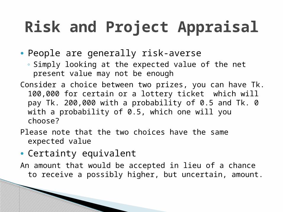
● People are generally risk-averse◦ Simply looking at the expected value of the net present

value may not be enough

Consider a choice between two prizes, you can have Tk. 100,000 for certain or a lottery ticket which will pay Tk. 200,000 with a probability of 0.5 and Tk. 0 with a probability of 0.5, which one will you choose?

Please note that the two choices have the same expected value

● Certainty equivalentAn amount that would be accepted in lieu of a chance to

receive a possibly higher, but uncertain, amount.

Risk and Project Appraisal

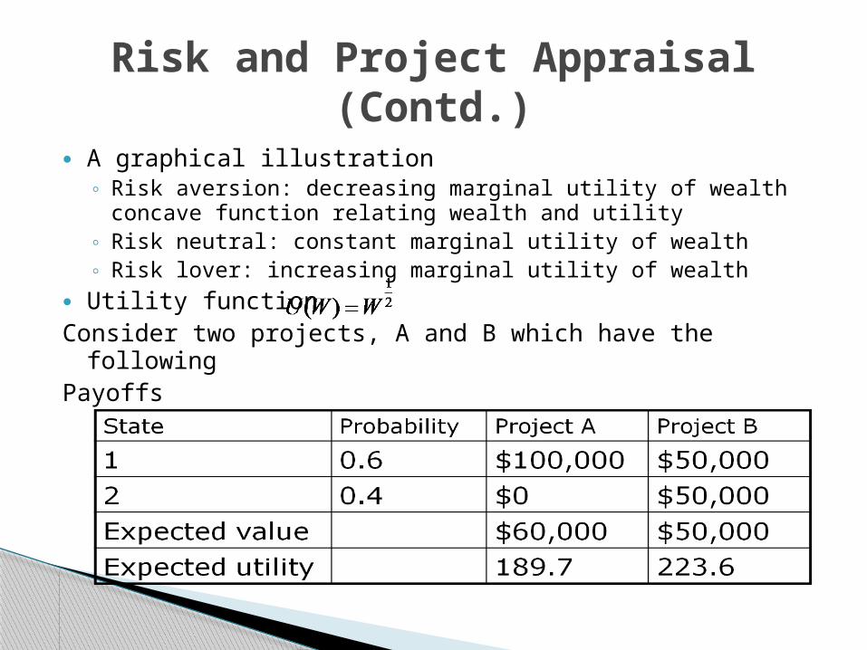
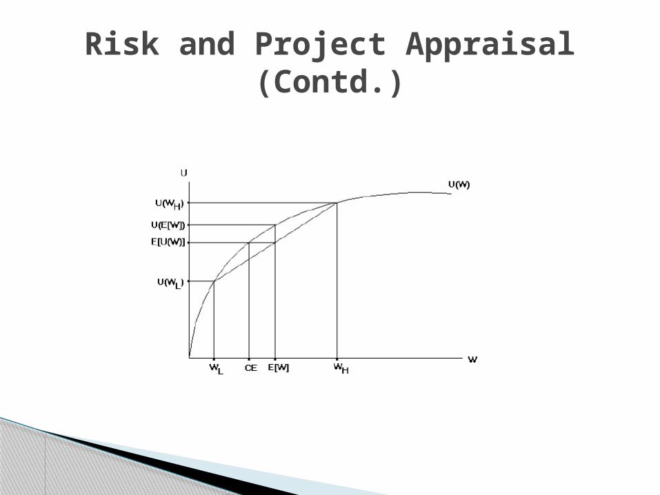
● A graphical illustration◦ Risk aversion: decreasing marginal utility of wealth concave

function relating wealth and utility◦ Risk neutral: constant marginal utility of wealth ◦ Risk lover: increasing marginal utility of wealth

● Utility functionConsider two projects, A and B which have the followingPayoffs

Risk and Project Appraisal (Contd.)

Risk and Project Appraisal (Contd.)

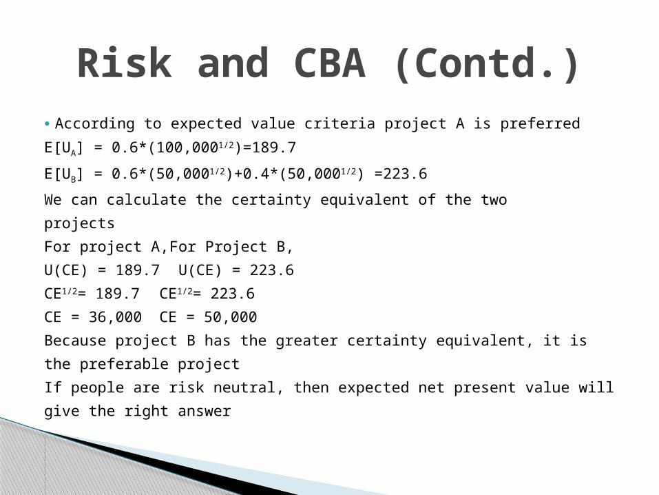
● According to expected value criteria project A is preferred

E[UA] = 0.6*(100,0001/2)=189.7

E[UB] = 0.6*(50,0001/2)+0.4*(50,0001/2) =223.6

We can calculate the certainty equivalent of the two

projects

For project A, For Project B,

U(CE) = 189.7 U(CE) = 223.6

CE1/2= 189.7 CE1/2= 223.6

CE = 36,000 CE = 50,000

Because project B has the greater certainty equivalent, it is

the preferable project

If people are risk neutral, then expected net present value will

give the right answer

Risk and CBA (Contd.)

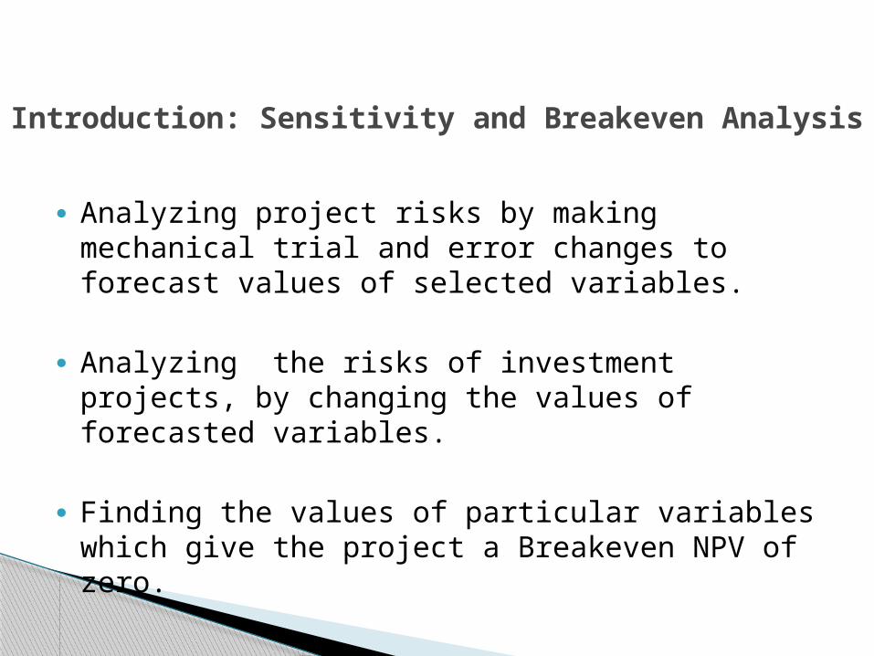
● Analyzing project risks by making mechanical trial and error changes to forecast values of selected variables.

● Analyzing the risks of investment projects, by changing the values of forecasted variables.

● Finding the values of particular variables which give the project a Breakeven NPV of zero.

Introduction: Sensitivity and Breakeven Analysis

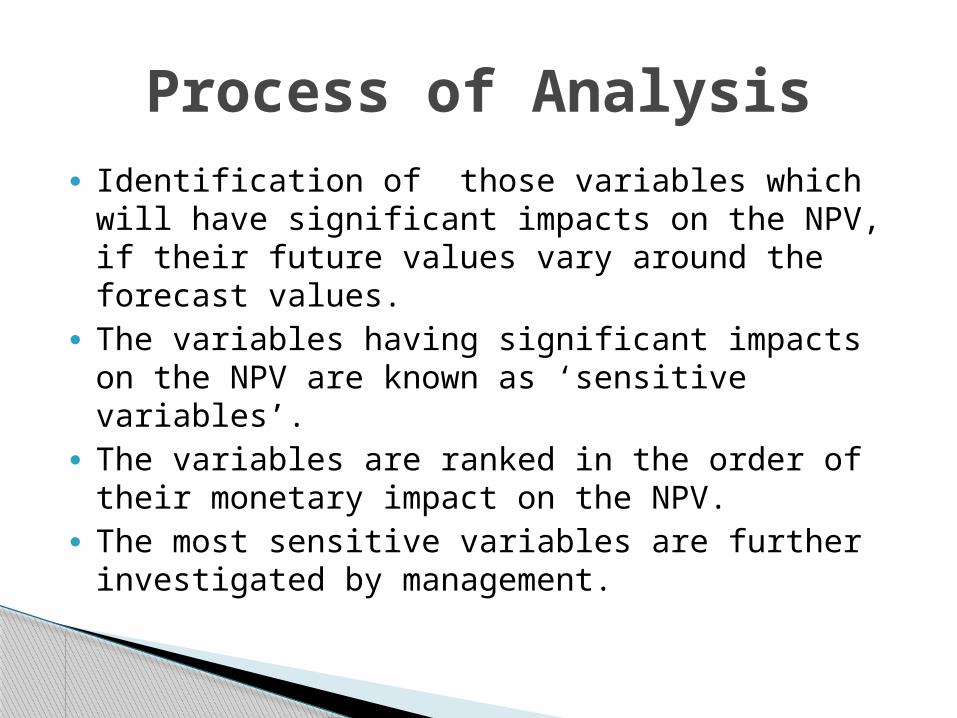
● Identification of those variables which will have significant impacts on the NPV, if their future values vary around the forecast values.

● The variables having significant impacts on the NPV are known as ‘sensitive variables’.

● The variables are ranked in the order of their monetary impact on the NPV.

● The most sensitive variables are further investigated by management.

Process of Analysis

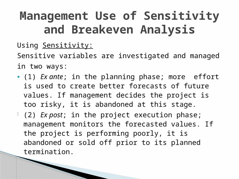
Using Sensitivity:

Sensitive variables are investigated and managed

in two ways:● (1) Ex ante; in the planning phase; more effort is used

to create better forecasts of future values. If management decides the project is too risky, it is abandoned at this stage.

• (2) Ex post; in the project execution phase; management monitors the forecasted values. If the project is performing poorly, it is abandoned or sold off prior to its planned termination.

Management Use of Sensitivity and Breakeven Analysis

Using Breakeven:• Forecasted calculated Breakeven values of

variables are continuously compared against actual outcomes during the execution phase.

Management Use of Sensitivity and Breakeven Analysis

● Sensitivity and Breakeven analyses are also known as: ‘scenario analysis’, and ‘what-if analysis’.

● Point values of forecasts are known as: ‘optimistic’, ‘most likely’, and ‘pessimistic’.

● Respective calculated NPVs are known as: ‘best case’, ‘base case’ and ‘worst case’.

● Variables giving a ‘breakeven’ value, return an NPV of zero for the project.

Terminology Within the Analysis

● Calculate the project’s NPV using the most likely

value estimated for each variable.

● Select from the set of uncertain variables those which

the management feels may have an important

bearing on predicted project performance.

● Forecast pessimistic, most likely, and optimistic

values for each of these variables over the life of the

project.

Steps in Sensitivity Analysis

● Recalculate the project’s NPV for each of these three

levels of each variable. While each particular variable

is stepped through each of its three values, all other

variables are held at their most likely values.

● Calculate the change in NPV for the pessimistic to

optimistic range of each variable.

● Identify sensitive variables.

Important: Selection of appropriate variables, and

establishing valid upper and lower forecast values.

Steps in Sensitivity Analysis

● Degree of management control.

● Management's confidence in the forecasts.

● Amount of management experience in assessing

projects.

● Extrinsic variables more problematic than

intrinsic variables.

● Time and cost of analysis.

Selection Criteria For Variables in the Analysis

● Large blowouts in initial construction costs for

Sydney Opera House, Montreal Olympic Stadium.

● Big budget films are shunned by critics and public

alike; e.g ‘Waterworld’: whilst cheap films

become classics; eg.‘Easy Rider’.

● High failure rate of rockets used to launch

commercial satellites.

Real Life Examples Forecast Errors

a) Use forecasting –error information from the forecasting methods: e.g. - upper and lower bounds; prediction interval; expert opinion; physical constraints, are applied to the variables.

This method is formalized, but arguable, slow and expensive.

Developing Optimistic and Pessimistic Forecasts

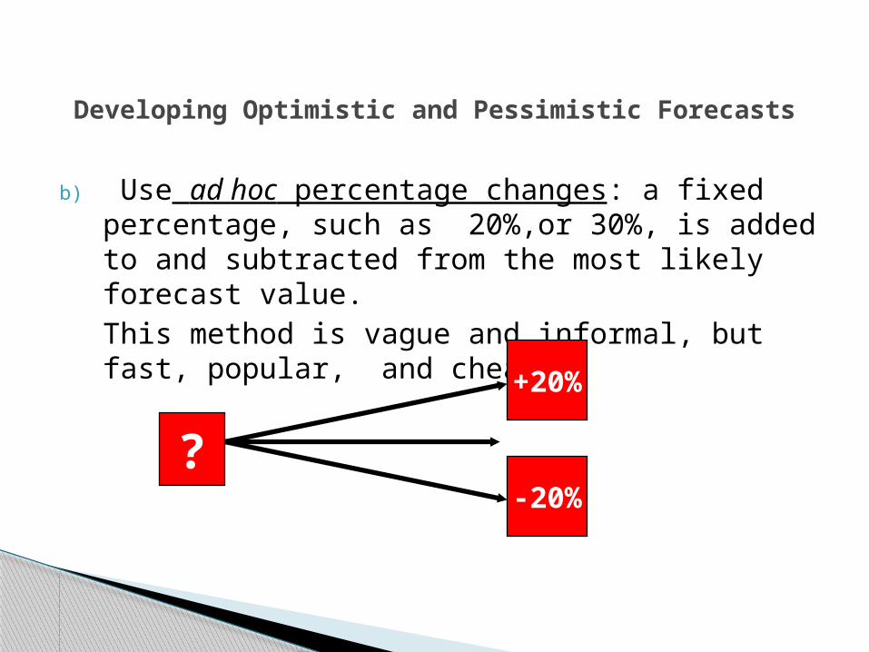
b) Use ad hoc percentage changes: a fixed percentage, such as 20%,or 30%, is added to and subtracted from the most likely forecast value.This method is vague and informal, but fast, popular, and cheap.

Developing Optimistic and Pessimistic Forecasts

?

+20%

-20%

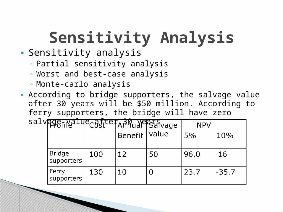
● Sensitivity analysis◦ Partial sensitivity analysis◦ Worst and best-case analysis◦ Monte-carlo analysis

● According to bridge supporters, the salvage value after 30 years will be $50 million. According to ferry supporters, the bridge will have zero salvage value after 30 years

Sensitivity Analysis

Sensitivity Analysis

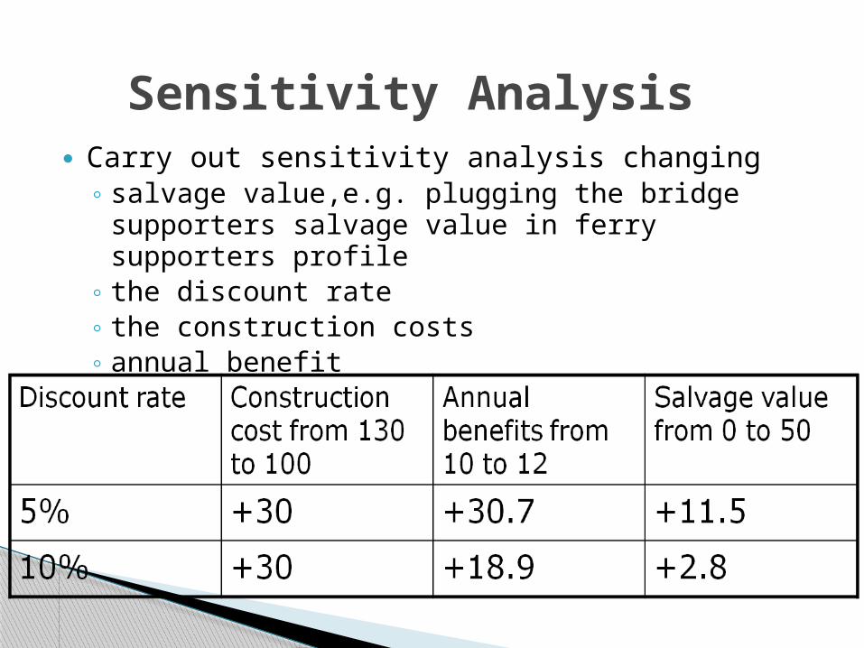
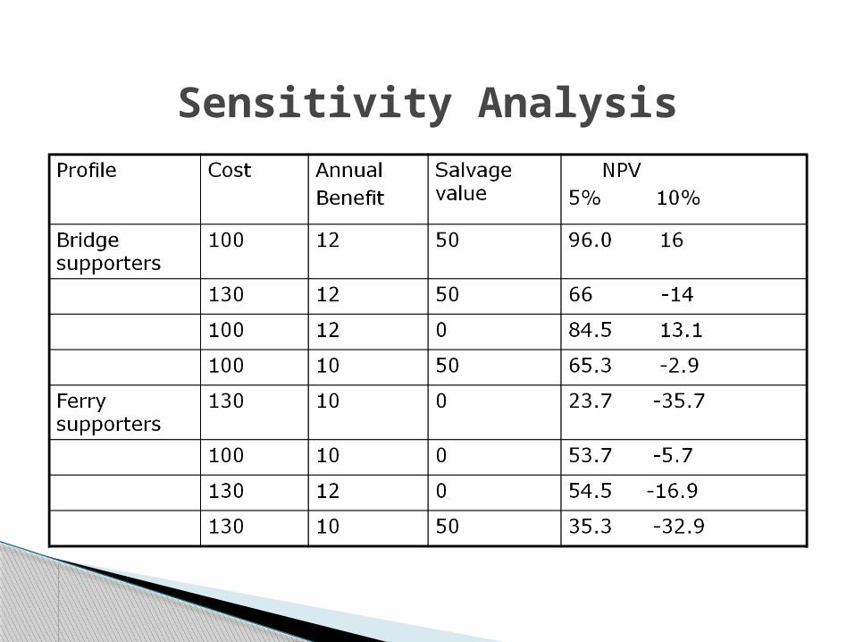
● Carry out sensitivity analysis changing ◦ salvage value,e.g. plugging the bridge supporters

salvage value in ferry supporters profile◦ the discount rate◦ the construction costs◦ annual benefit

Sensitivity Analysis

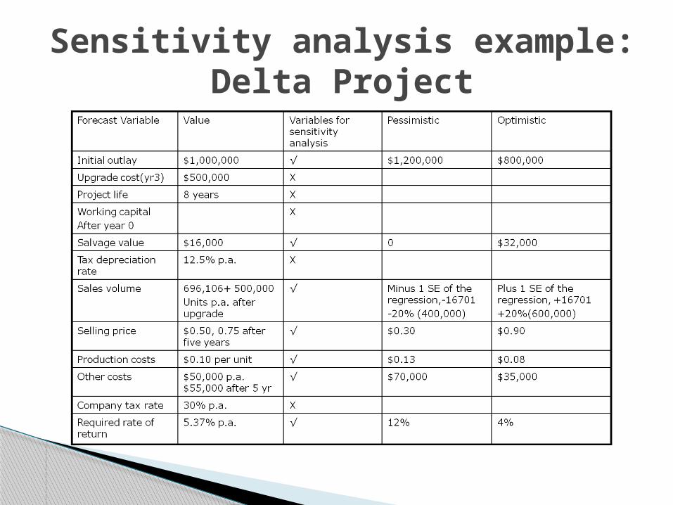
Sensitivity analysis example: Delta Project

Workbook8.1.xls

Delta Project: Sensitivity Analysis Results

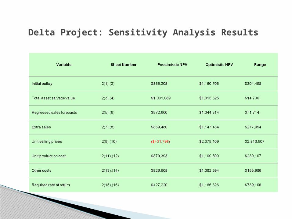
Delta Project: Sensitivity Analysis Results

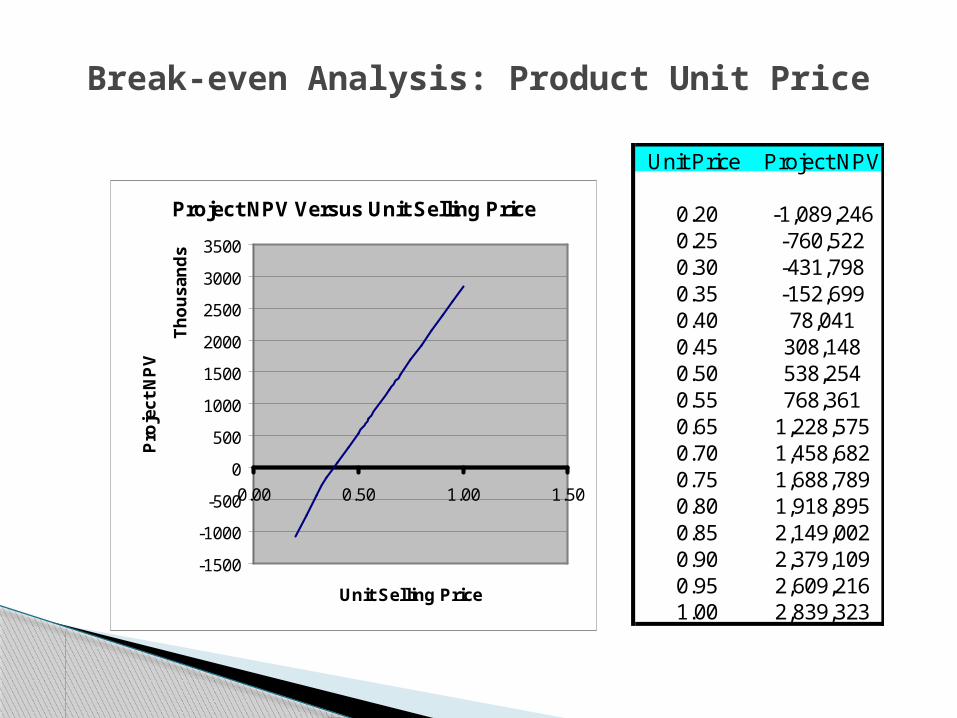
Unit Price Project NPV

0.20 -1,089,2460.25 -760,5220.30 -431,7980.35 -152,6990.40 78,0410.45 308,1480.50 538,2540.55 768,3610.65 1,228,5750.70 1,458,6820.75 1,688,7890.80 1,918,8950.85 2,149,0020.90 2,379,1090.95 2,609,2161.00 2,839,323

Project NPV Versus Unit Selling Price

-1500

-1000

-500

0

500

1000

1500

2000

2500

3000

3500

0.00 0.50 1.00 1.50

Th

ou

san

ds

Unit Selling Price

Pro

ject

NP

V

Break-even Analysis: Product Unit Price

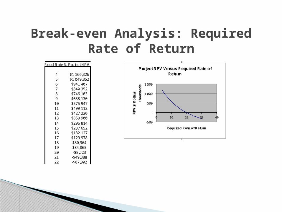
Reqd Rate % Project NPV

4 $1,166,3265 $1,049,8526 $941,4077 $840,3528 $746,1039 $658,13010 $575,94711 $499,11212 $427,22013 $359,90014 $296,81415 $237,65216 $182,12717 $129,97818 $80,96419 $34,86520 -$8,52321 -$49,38822 -$87,902

Project NPV Versus Required Rate of Return

-500

-

500

1,000

1,500

0 10 20 30 40

Th

ou

sa

nd

s

Required Rate of Return

NP

V i

n D

oll

ars

Break-even Analysis: Required Rate of Return

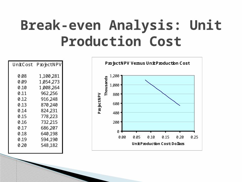
Unit Cost Project NPV

0.08 1,100,2810.09 1,054,2730.10 1,008,2640.11 962,2560.12 916,2480.13 870,2400.14 824,2310.15 778,2230.16 732,2150.17 686,2070.18 640,1980.19 594,1900.20 548,182

Project NPV Versus Unit Production Cost

0

200

400

600

800

1,000

1,200

0.00 0.05 0.10 0.15 0.20 0.25

Th

ou

san

ds

Unit Production Cost: Dollars

Pro

ject

NP

V

Break-even Analysis: Unit Production Cost

● Each forecast value is entered into the model, and one solution is given.

● Solutions can be summarized automatically, or individually by hand.

● Variables are ranked in order of the monetary range of calculated NPVs.

● Management investigates the sensitive variables.● More forecasting is done, or the project is

accepted or rejected as is.

Outputs and Uses

● Strengths:◦ Easy to understand.◦ Forces planning discipline.◦ Helps to highlight risky variables.◦ Relatively cheap.

● Weaknesses ◦ Relatively unsophisticated.◦ May not capture all information.◦ Limited to one variable at a time.◦ Ignores interdependencies.

Strengths and Weaknesses of Analysis

● Project risk analysis by simultaneous adjustment of

forecast values.

● Simulation allows the repeated solution of an

evaluation model.

● Each solution randomly selects values from

predetermined probability distributions.

● All solutions are summarized into an overall

distribution of NPV values.

● This distribution shows management how risky the

project is.

Simulation: an Introduction

● The treatment of risk by using simulation is known as

‘stochastic’ modeling.

● Other names for our term ‘Simulation’, are - ‘Risk

Analysis’, ‘Venture Analysis’,’Risk Simulation’, ‘Monte

Carlo Simulation’.

● The name ‘Monte Carlo Simulation’ helps

visualization of repeated spins of the roulette wheel,

creating the selected values.

● Each execution of the model is known as a

‘replication’ or ‘iteration’.

Simulation Terminology

● Follows the initial creation and basic testing of the

representative model.

● Is sometimes used as a test of the model.

● Emphasizes the need for formal forecasting, and

requires close specification of the forecast

variables.

● Draws managements attention to the inherent risk

in any project.

● Focuses attention on accurate model building.

The Role of Simulation

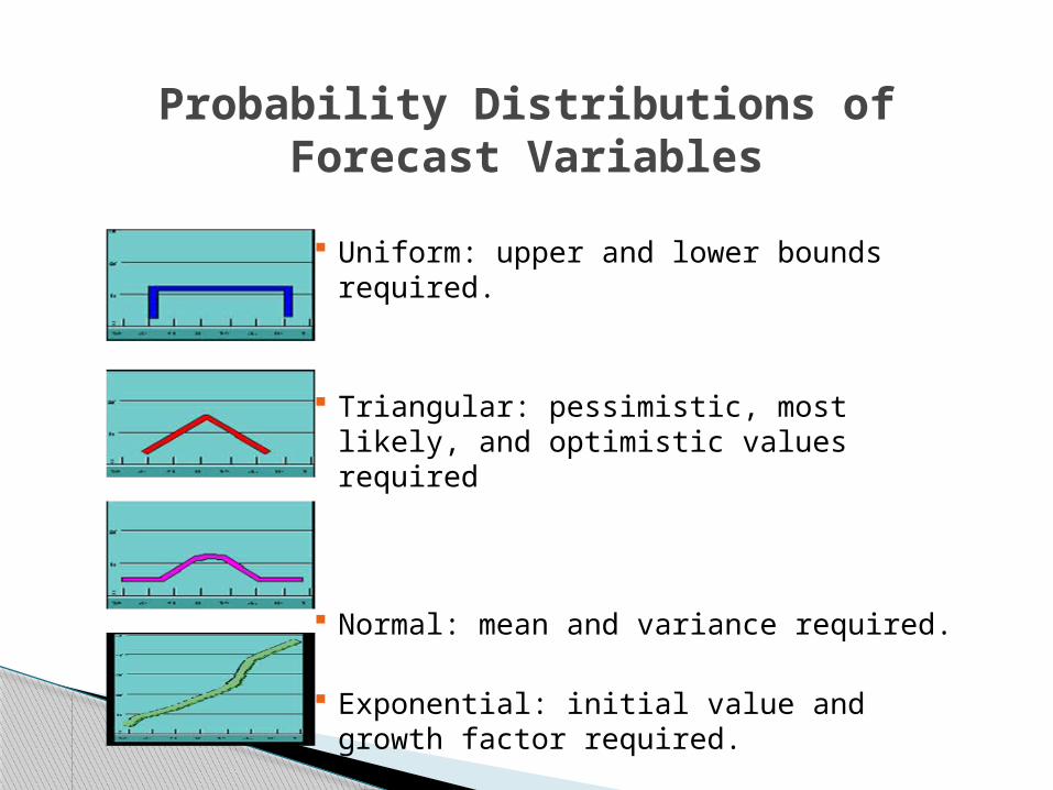
Uniform: upper and lower bounds required.

Triangular: pessimistic, most likely, and optimistic values required

Normal: mean and variance required.

Exponential: initial value and growth factor required.

Probability Distributions of Forecast Variables

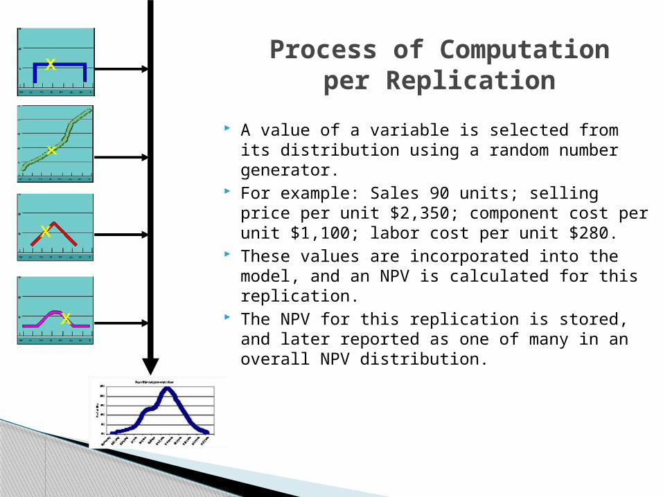
Process of Computation per Replication

A value of a variable is selected from its distribution using a random number generator.

For example: Sales 90 units; selling price per unit $2,350; component cost per unit $1,100; labor cost per unit $280.

These values are incorporated into the model, and an NPV is calculated for this replication.

The NPV for this replication is stored, and later reported as one of many in an overall NPV distribution.

● Each replication is unique.

● Selection of values from the distribution is made

according to the particular distributions

● The automated process is driven by a random number

generator.

● Excel add-ons such as ‘@Risk’ and ‘Insight’ can be

used to streamline the process.

● About 500 replications should give a good picture of

the project’s risk.

Making the Replications

● Management can view the risk of the project.

● Probability of generating an NPV between two given values can be calculated.

● Probability of loss is the area to the left of a zero NPV.

Using the Output

● Benefits

◦ Focuses on a detailed definition and analysis of risk.

◦ Sophisticated analysis clearly portrays the risk of a project

◦ Gives the probability of a loss making project

◦ Allows simultaneous analysis of variables

● Costs

◦ Requires a significant forecasting effort.

◦ Can be difficult to set up for computation.

◦ Output can be difficult to interpret.

Benefits and Costs of Simulation

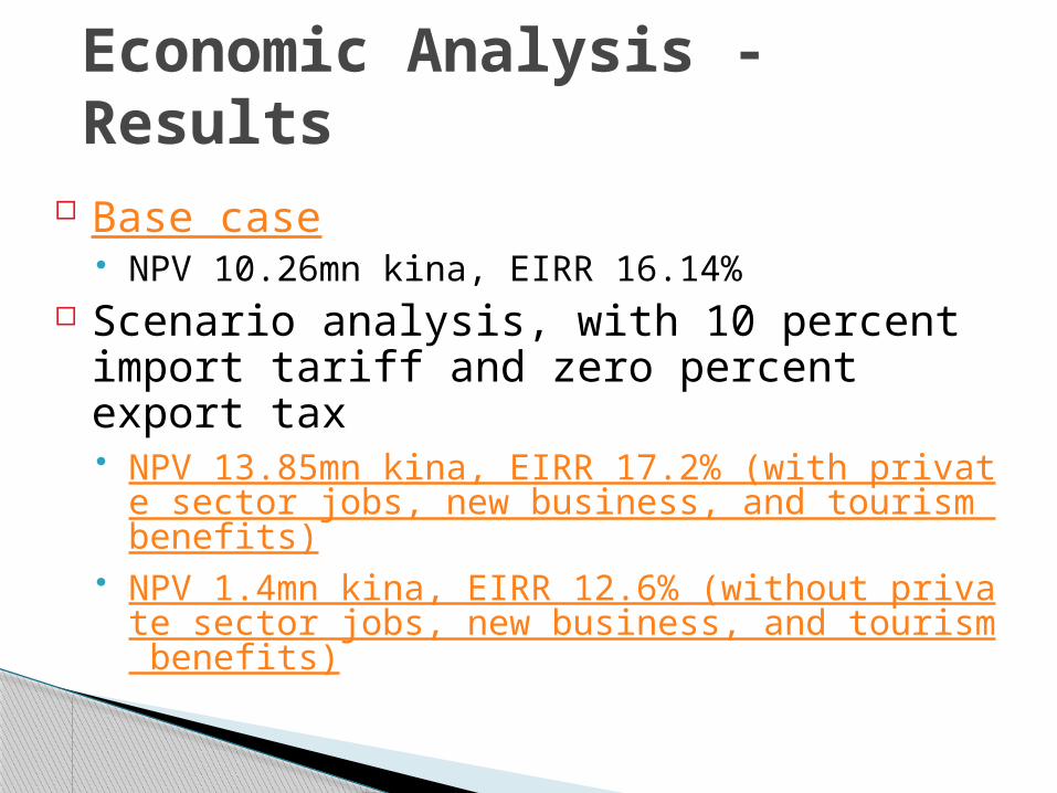
Economic Analysis -Results

Base case NPV 10.26mn kina, EIRR 16.14%

Scenario analysis, with 10 percent import tariff and zero percent export tax NPV 13.85mn kina, EIRR 17.2% (with private sector job

s, new business, and tourism benefits) NPV 1.4mn kina, EIRR 12.6% (without private sector job

s, new business, and tourism benefits)

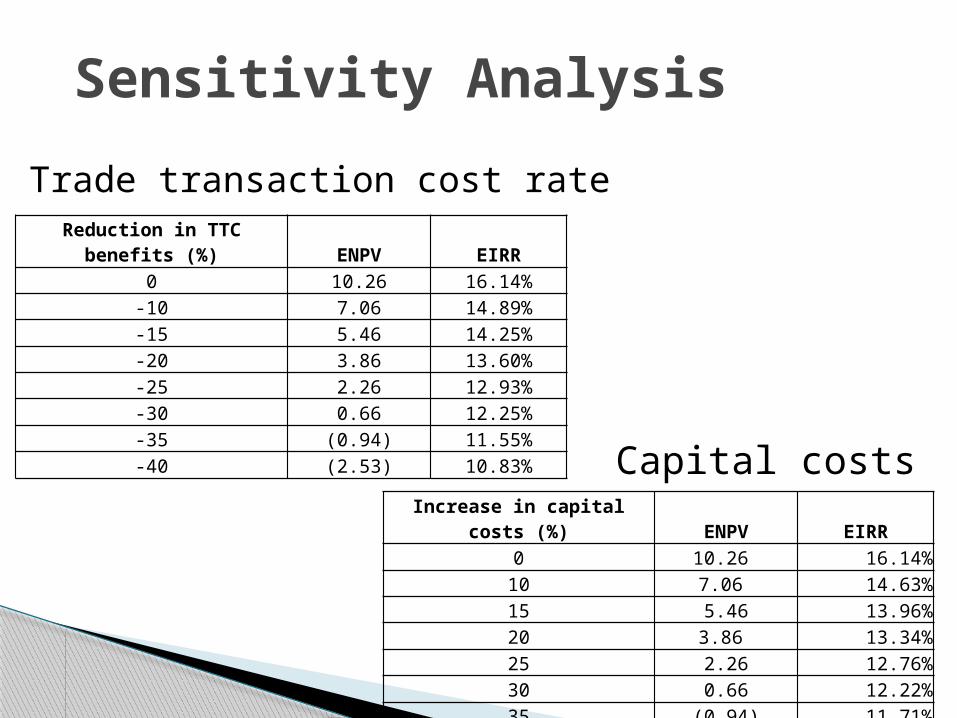
Sensitivity Analysis

Reduction in TTC benefits (%) ENPV EIRR0 10.26 16.14%

-10 7.06 14.89%-15 5.46 14.25%-20 3.86 13.60%-25 2.26 12.93%-30 0.66 12.25%-35 (0.94) 11.55%-40 (2.53) 10.83%

Trade transaction cost rate

Capital costsIncrease in capital costs (%) ENPV EIRR

0 10.26 16.14%10 7.06 14.63%15 5.46 13.96%20 3.86 13.34%25 2.26 12.76%30 0.66 12.22%35 (0.94) 11.71%40 (2.53) 11.22%

Sensitivity Analysis

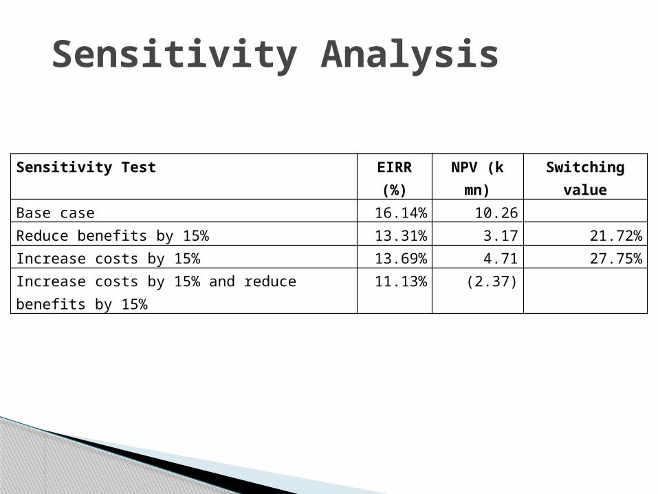
Sensitivity Test EIRR (%) NPV (k mn) Switching value

Base case 16.14% 10.26Reduce benefits by 15% 13.31% 3.17 21.72%Increase costs by 15% 13.69% 4.71 27.75%Increase costs by 15% and reduce benefits by 15% 11.13% (2.37)

Monte Carlo Simulation

Monte Carlo simulation conducted using four variables, which are:◦ Reduction in trade transaction costs◦ Capital costs◦ Import tariff◦ Benefits from social development program

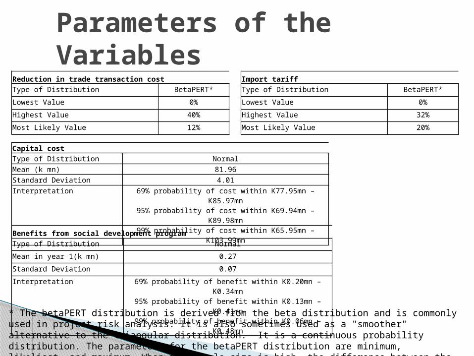
Parameters of the Variables

Reduction in trade transaction costType of Distribution BetaPERT*

Lowest Value 0%

Highest Value 40%

Most Likely Value 12%

Capital costType of Distribution NormalMean (k mn) 81.96Standard Deviation 4.01Interpretation 69% probability of cost within K77.95mn – K85.97mn

95% probability of cost within K69.94mn – K89.98mn99% probability of cost within K65.95mn – K103.99mn

Benefits from social development programType of Distribution Normal

Mean in year 1(k mn) 0.27

Standard Deviation 0.07

Interpretation 69% probability of benefit within K0.20mn – K0.34mn95% probability of benefit within K0.13mn – K0.41mn99% probability of benefit within K0.06mn – K0.48mn

Import tariffType of Distribution BetaPERT*

Lowest Value 0%

Highest Value 32%

Most Likely Value 20%

* The betaPERT distribution is derived from the beta distribution and is commonly used in project risk analysis. It is also sometimes used as a "smoother" alternative to the triangular distribution. It is a continuous probability distribution. The parameters for the betaPERT distribution are minimum, likeliest, and maximum. When the sample size is high, the difference between the normal distribution and BetaPERT distribution is the kurtosis.

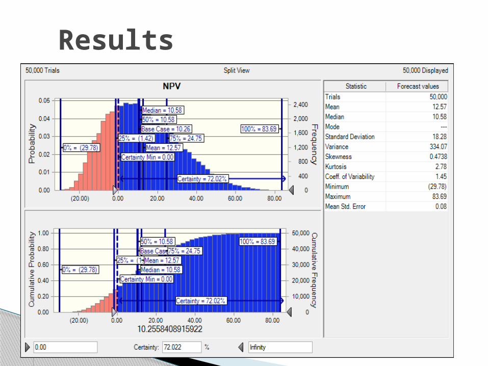
Results

Interpretation of the results

NPV varies from –K29.78mn to K83.69mn. Probability of NPV being positive is 72.02% and

negative is 17.98%. Mean NPV is K12.57mn and median NPV is

K10.58mn. Both are higher than the base case. It shows that, the base was rather

conservative. The probability of a ‘conservative’ base case

delivering positive NPV is very high, meaning that the project is fundamentally sound.

The project is highly influenced by the changes in reduction in trade transaction cost.