Embed Size (px)
DESCRIPTION
Simplified Method of Modeling Complex Systems of Simple Optics using Wave-Optics: An Engineering Approach. Dr. Justin D. Mansell, Steve Coy, Liyang Xu, Anthony Seward, and Robert Praus MZA Associates Corporation. Outline. Introduction Ray Matrices Lens Law Fourier Optics - PowerPoint PPT Presentation
Citation preview
1
Simplified Method of Modeling Complex Systems
of Simple Optics using Wave-Optics:
An Engineering ApproachDr. Justin D. Mansell, Steve Coy, Liyang Xu,
Anthony Seward, and Robert Praus
MZA Associates Corporation
2
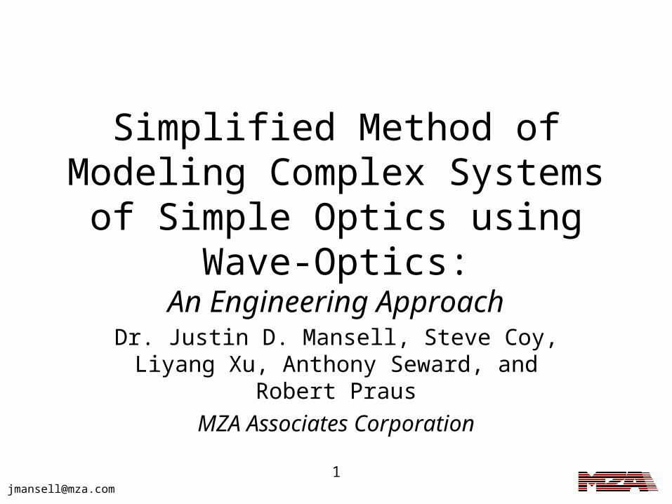
Outline• Introduction
– Ray Matrices– Lens Law– Fourier Optics
• Aperture Imaging Into Input Space
• Finding the Field Stop & Aperture Stop
• Mesh Determination for Complex Systems
• Conclusions
4
Introduction - ABCD Matrices
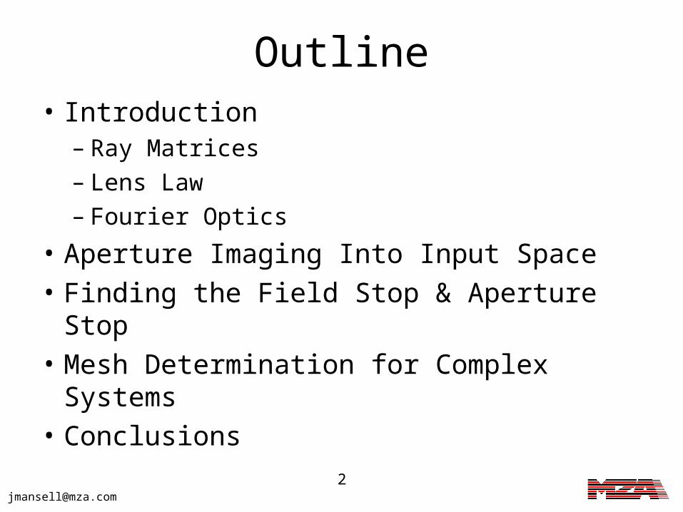
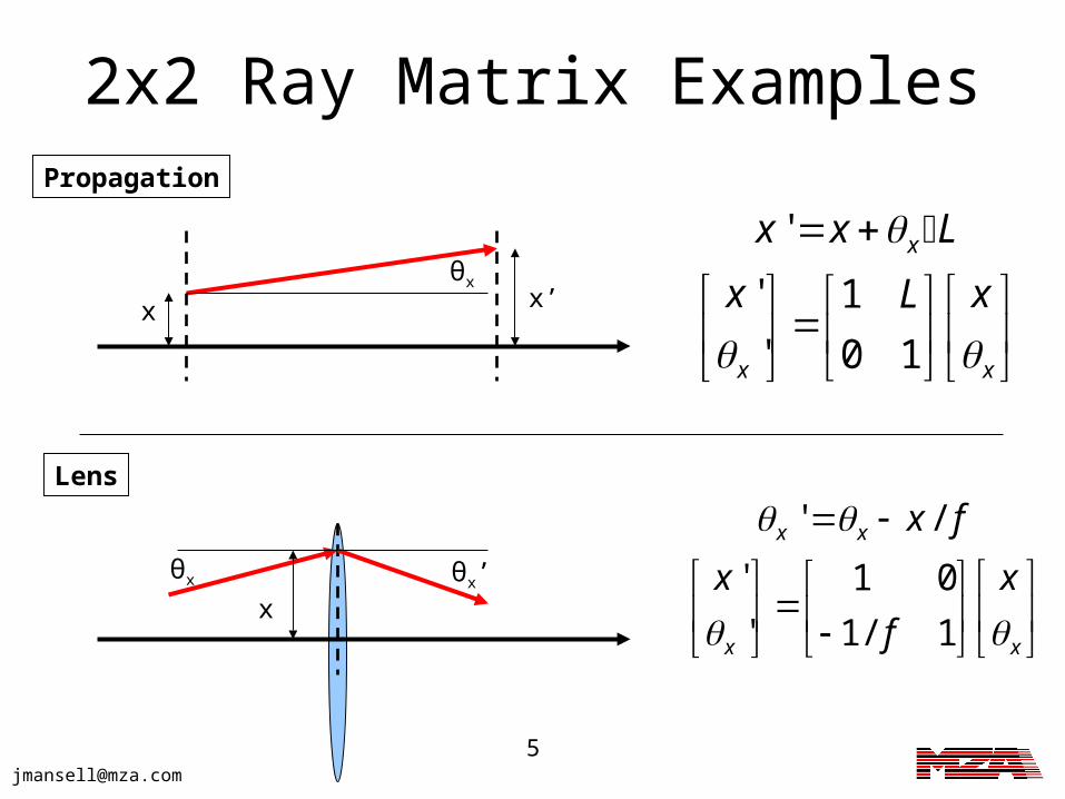
• The most common ray matrix formalism is the 2x2 or ABCD that describes how a ray height, x, and angle, θx, changes through a system.
θx
xA B
C D
θx’x’
'
'
'
'
x x
x
x x
x xA B
C D
x Ax B
Cx D
5
2x2 Ray Matrix ExamplesPropagation
Lens
θx
x x’
'
' 1
' 0 1
x
x x
x x L
x xL
θx
x
' /
' 1 0
' 1/ 1
x x
x x
x f
x x
f
θx’
6
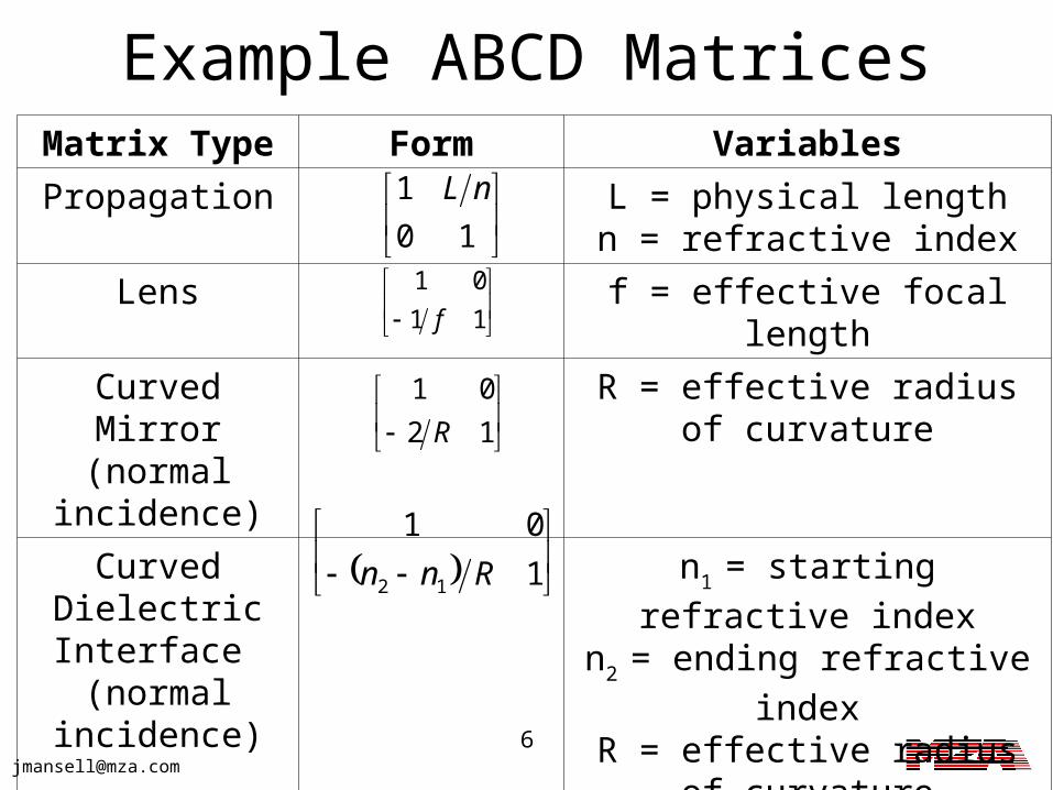
Example ABCD MatricesMatrix Type Form Variables
Propagation L = physical lengthn = refractive index
Lens f = effective focal length
Curved Mirror(normal
incidence)
R = effective radius of curvature
Curved Dielectric Interface (normal
incidence)
n1 = starting refractive index
n2 = ending refractive index
R = effective radius of curvature
10
1 nL
11
01
f
12
01
R
1
01
12 Rnn
7
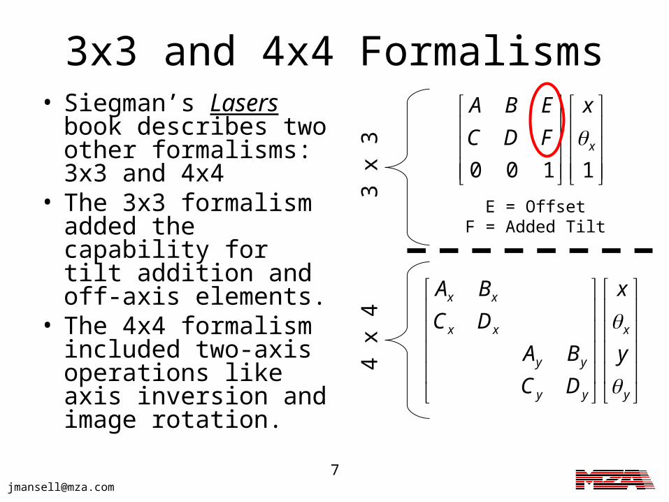
3x3 and 4x4 Formalisms• Siegman’s Lasers
book describes two other formalisms: 3x3 and 4x4
• The 3x3 formalism added the capability for tilt addition and off-axis elements.
• The 4x4 formalism included two-axis operations like axis inversion and image rotation.
0 0 1 1x
A B E x
C D F
x x
x x x
y y
y y y
A B x
C D
A B y
C D
E = OffsetF = Added Tilt
3 x
34
x 4
8
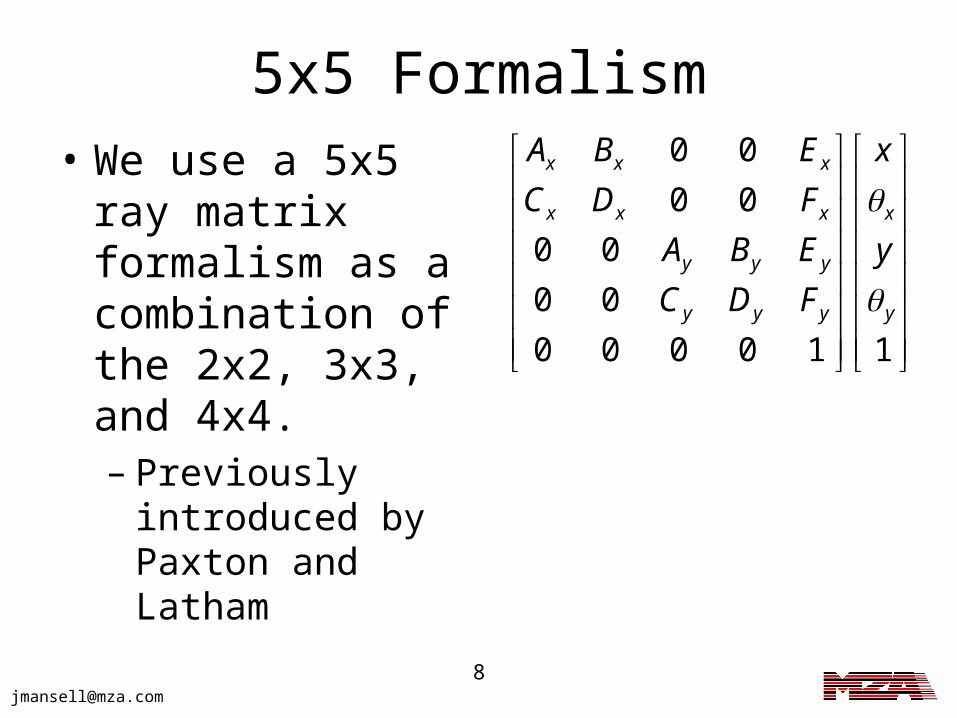
5x5 Formalism• We use a 5x5 ray
matrix formalism as a combination of the 2x2, 3x3, and 4x4.– Previously
introduced by Paxton and Latham
0 0
0 0
0 0
0 0
0 0 0 0 1 1
x x x
x x x x
y y y
y y y y
A B E x
C D F
A B E y
C D F
9
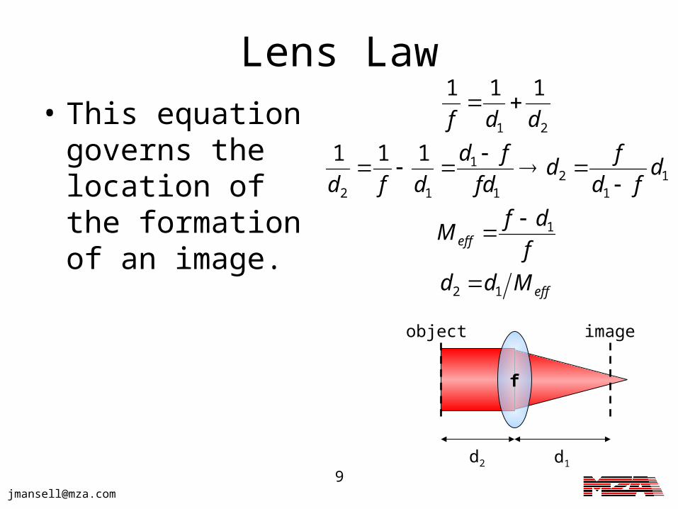
Lens Law• This equation
governs the location of the formation of an image.
eff
eff
Mdd
f
dfM
dfd
fd
fd
fd
dfd
ddf
12
1
11
21
1
12
21
111
111
f
d2 d1
object image
10
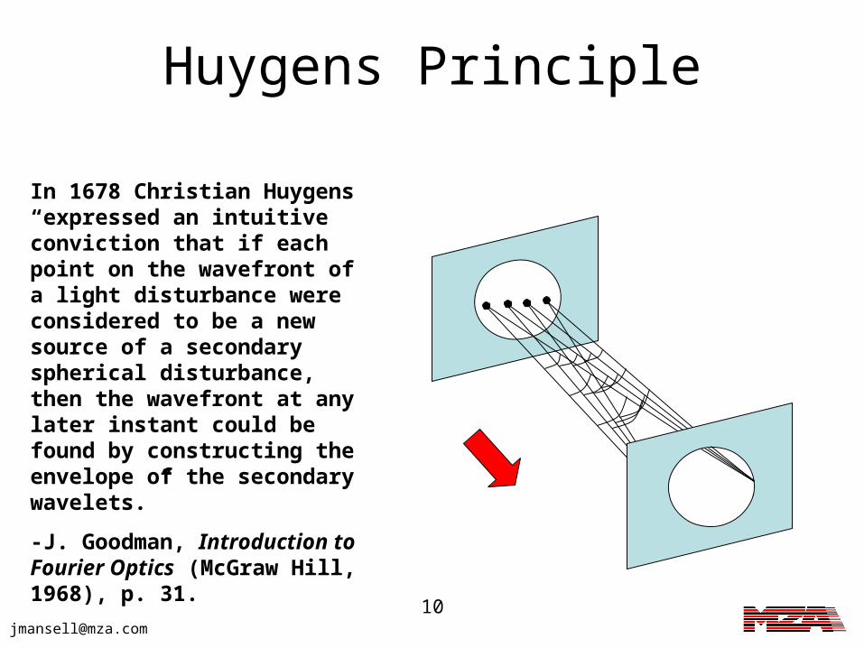
Huygens Principle
In 1678 Christian Huygens “expressed an intuitive conviction that if each point on the wavefront of a light disturbance were considered to be a new source of a secondary spherical disturbance, then the wavefront at any later instant could be found by constructing the envelope of the secondary wavelets.”
-J. Goodman, Introduction to Fourier Optics (McGraw Hill, 1968), p. 31.
11
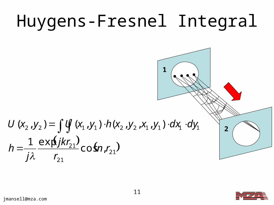
Huygens-Fresnel Integral
2121
21
1111221122
,cosexp1
),,,(),(),(
rnr
jkr
jh
dydxyxyxhyxUyxU
1
2

12
Fresnel Approximation
• Fresnel found that in modeling longer propagations, – the cosine term
could be neglected and
– the spherical term could be approximated by a r2 term.
2121
21
1111221122
,cosexp1
),,,(),(),(
rnr
jkr
jh
dydxyxyxhyxUyxU
Huygens-Fresnel Integral
Fresnel Approximation
22a
111212
21
11
22
22
r where
exp
2exp),(
2exp
)exp(),(
aa yx
dydxyyxxz
kj
z
rjkyxU
z
rjk
jkz
jkzyxU
13
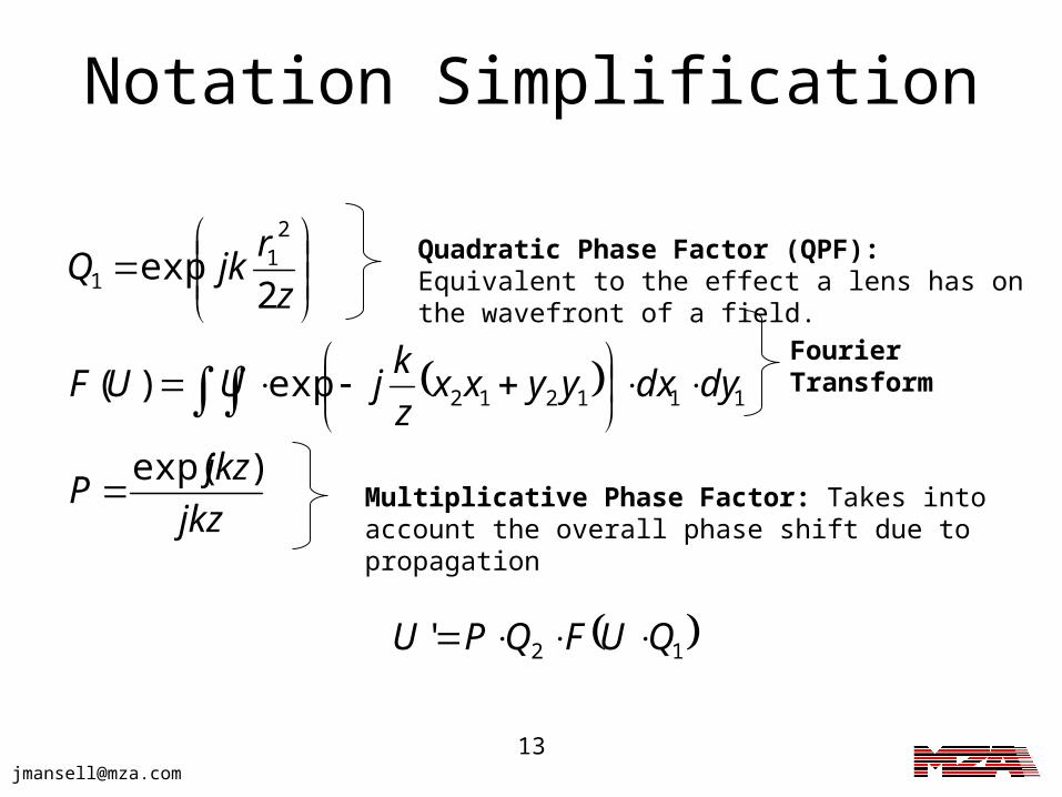
Notation Simplification
jkz
jkzP
dydxyyxxz
kjUUF
z
rjkQ
)exp(
exp)(
2exp
111212
21
1
Quadratic Phase Factor (QPF): Equivalent to the effect a lens has on the wavefront of a field.
Fourier Transform
Multiplicative Phase Factor: Takes into account the overall phase shift due to propagation
12' QUFQPU
14
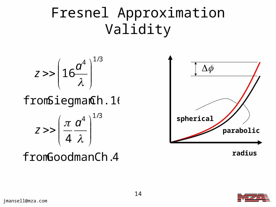
Fresnel Approximation Validity
4 Ch.Goodman from
4
Ch.16Siegman from
16
3/14
3/14
az
az
radius
spherical
parabolic
15
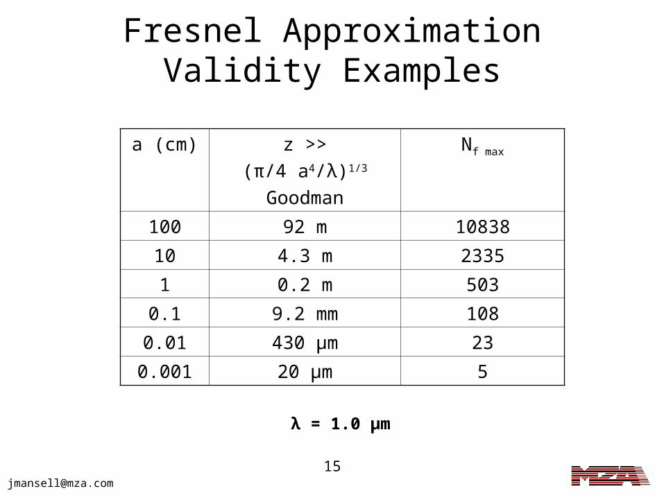
Fresnel Approximation Validity Examples
a (cm) z >>
(π/4 a4/λ)1/3
Goodman
Nf max
100 92 m 10838
10 4.3 m 2335
1 0.2 m 503
0.1 9.2 mm 108
0.01 430 μm 23
0.001 20 μm 5
λ = 1.0 μm
16
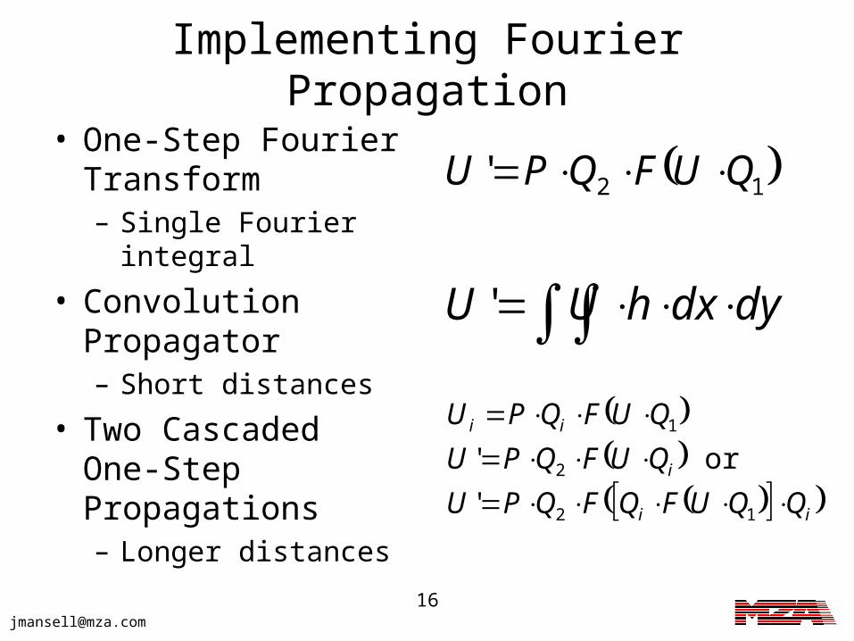
Implementing Fourier Propagation
• One-Step Fourier Transform– Single Fourier integral
• Convolution Propagator – Short distances
• Two Cascaded One-Step Propagations– Longer distances
12' QUFQPU
dydxhUU '
ii
i
ii
QQUFQFQPU
QUFQPU
QUFQPU
12
2
1
'
or '
17
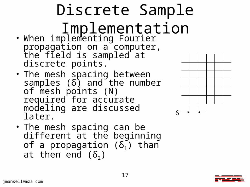
Discrete Sample Implementation
• When implementing Fourier propagation on a computer, the field is sampled at discrete points.
• The mesh spacing between samples (δ) and the number of mesh points (N) required for accurate modeling are discussed later.
• The mesh spacing can be different at the beginning of a propagation (δ1) than at then end (δ2)
δ
18
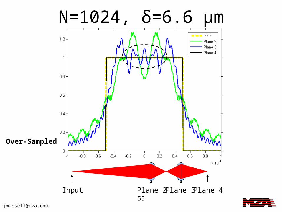
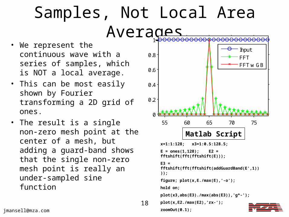
Samples, Not Local Area Averages
• We represent the continuous wave with a series of samples, which is NOT a local average.
• This can be most easily shown by Fourier transforming a 2D grid of ones.
• The result is a single non-zero mesh point at the center of a mesh, but adding a guard-band shows that the single non-zero mesh point is really an under-sampled sine function
x=1:1:128; x3=1:0.5:128.5;
E = ones(1,128); E2 = fftshift(fft(fftshift(E)));
E3 = fftshift(fft(fftshift(addGuardBand(E',1))));
figure; plot(x,E./max(E),'-o');
hold on;
plot(x3,abs(E3)./max(abs(E3)),'g*-');
plot(x,E2./max(E2),'rx-');
zoomOut(0.1);
Matlab Script
55 60 65 70 75
0
0.2
0.4
0.6
0.8
1
Input
FFTFFT w GB
19
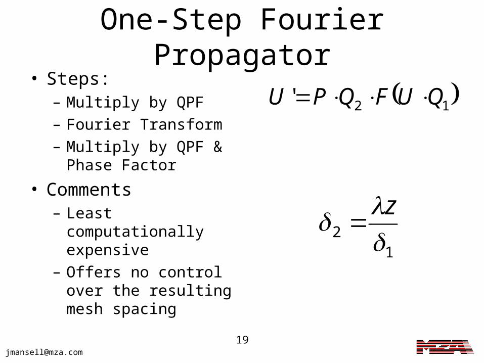
One-Step Fourier Propagator• Steps:
– Multiply by QPF– Fourier Transform– Multiply by QPF &
Phase Factor
• Comments– Least computationally
expensive– Offers no control over
the resulting mesh spacing
12
z
12' QUFQPU
20
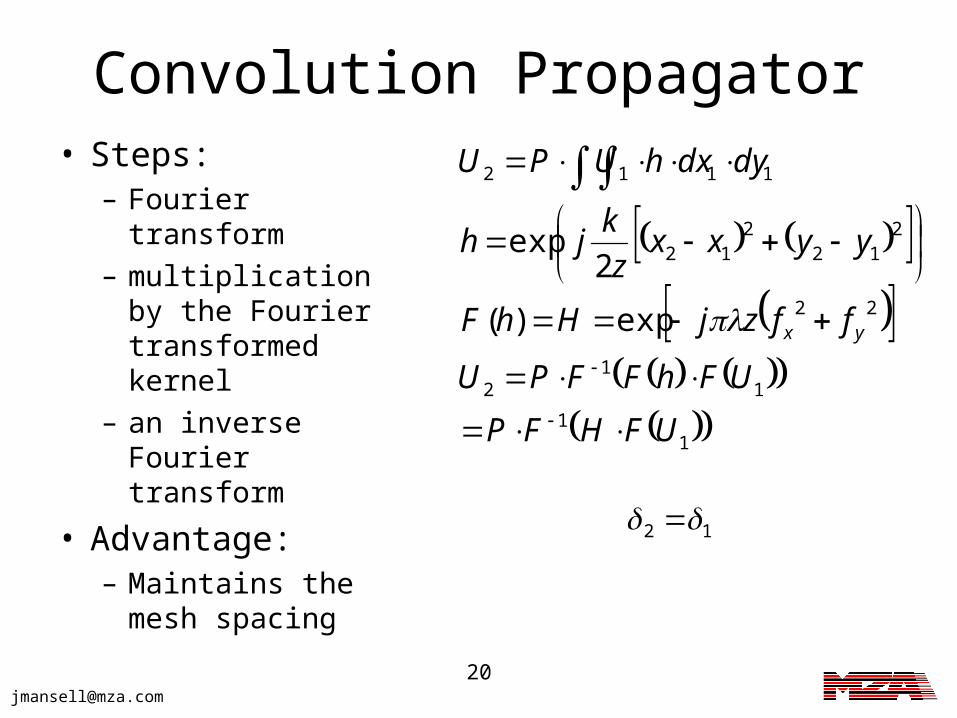
Convolution Propagator• Steps:
– Fourier transform– multiplication by
the Fourier transformed kernel
– an inverse Fourier transform
• Advantage:– Maintains the
mesh spacing
1
1
11
2
22
212
212
1112
exp)(
2exp
UFHFP
UFhFFPU
ffzjHhF
yyxxz
kjh
dydxhUPU
yx
12
21
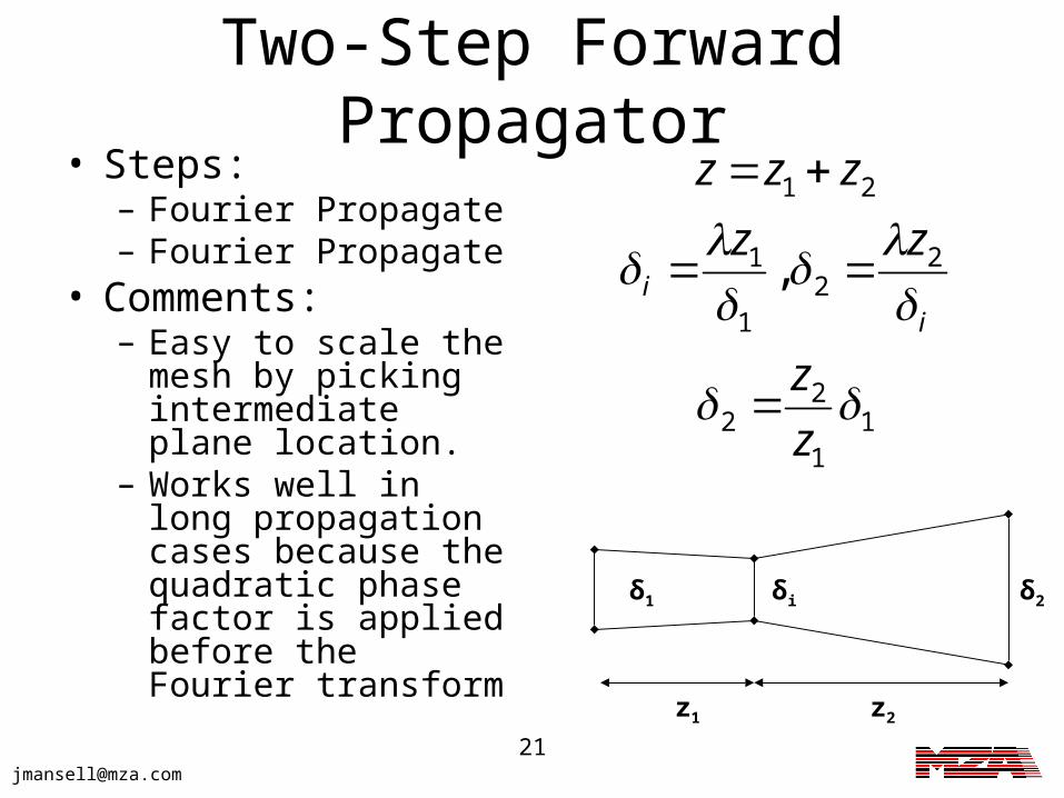
Two-Step Forward Propagator
• Steps:– Fourier Propagate– Fourier Propagate
• Comments:– Easy to scale the mesh
by picking intermediate plane location.
– Works well in long propagation cases because the quadratic phase factor is applied before the Fourier transform
11
22
22
1
1
21
,
z
z
zz
zzz
ii
z1 z2
δ1 δ2δi
22
Scaling with the Convolution Propagator
• One drawback of the convolution propagator is its apparent inability to scale the mesh spacing in a propagation.
• Scaling the mesh is important when propagating with significant wavefront curvature.
• The convolution propagator can be modified to model propagation relative to a spherical reference wavefront curvature such that the mesh spacing can follow the curvature of the wavefront.
• We call this Spherical-Reference Wave Propagation or SWP.
23
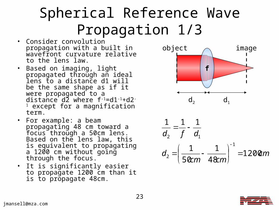
Spherical Reference Wave Propagation 1/3
• Consider convolution propagation with a built in wavefront curvature relative to the lens law.
• Based on imaging, light propagated through an ideal lens to a distance d1 will be the same shape as if it were propagated to a distance d2 where f-1=d1-1+d2-1 except for a magnification term.
• For example: a beam propagating 48 cm toward a focus through a 50cm lens. Based on the lens law, this is equivalent to propagating a 1200 cm without going through the focus.
• It is significantly easier to propagate 1200 cm than it is to propagate 48cm.
f
d2 d1
object image
cmcmcm
d
dfd
120048
1
50
1
111
1
2
12
24
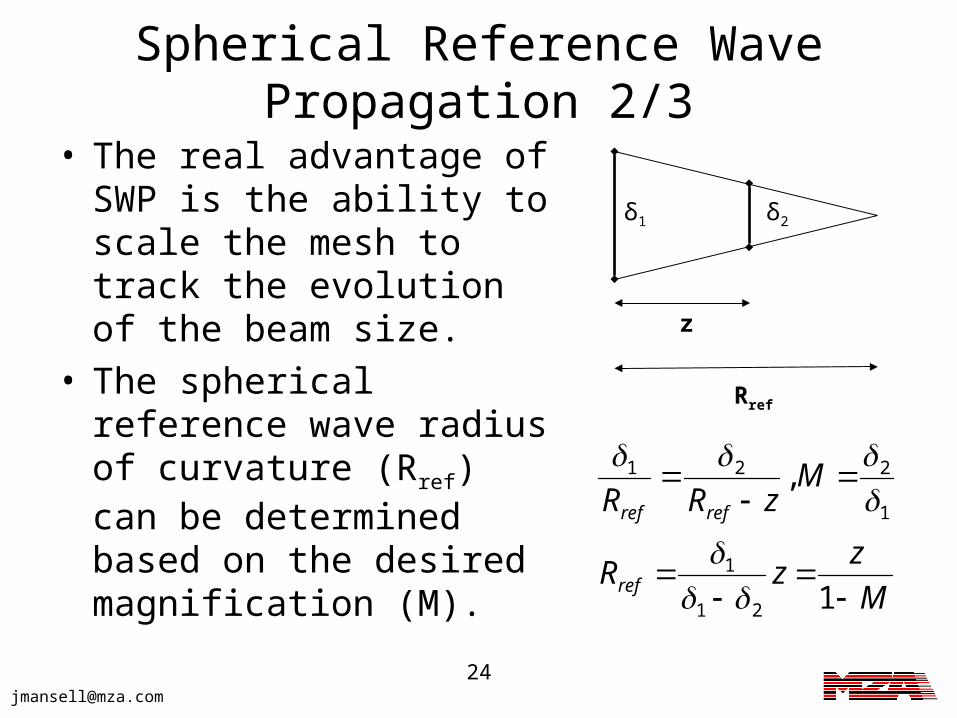
Spherical Reference Wave Propagation 2/3
• The real advantage of SWP is the ability to scale the mesh to track the evolution of the beam size.
• The spherical reference wave radius of curvature (Rref) can be determined based on the desired magnification (M).
z
Rref
δ1 δ2
M
zzR
MzRR
ref
refref
1
,
21
1
1
221
25
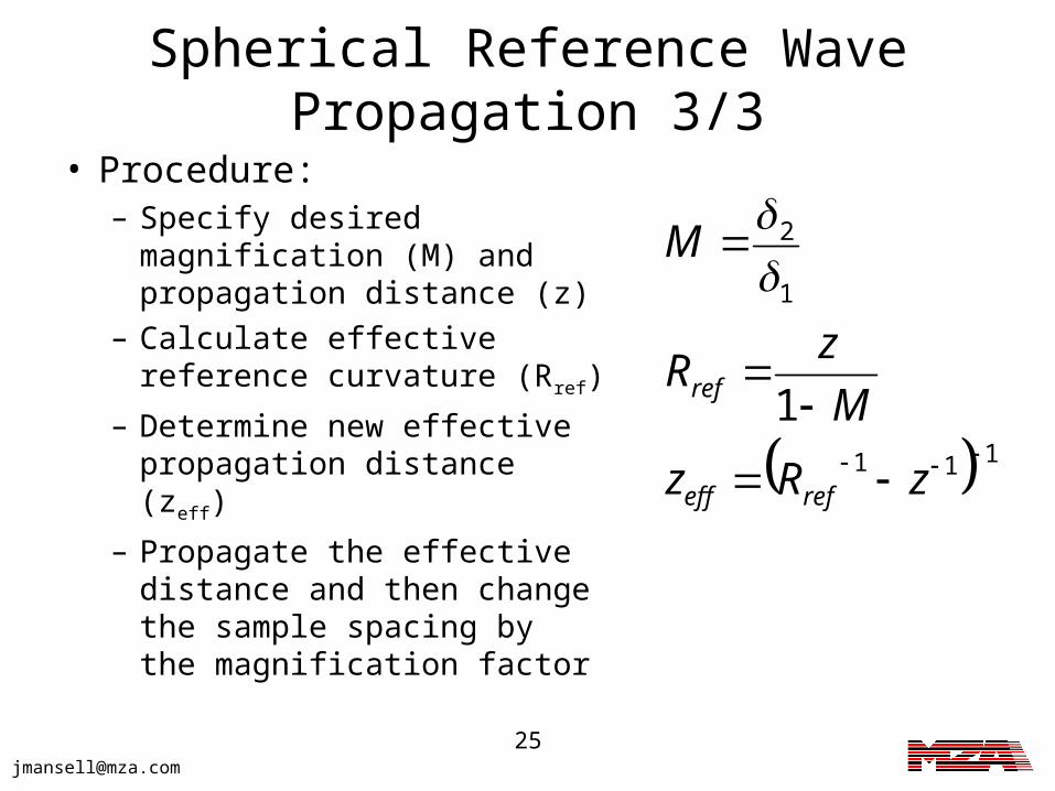
Spherical Reference Wave Propagation 3/3
• Procedure:– Specify desired
magnification (M) and propagation distance (z)
– Calculate effective reference curvature (Rref)
– Determine new effective propagation distance (zeff)
– Propagate the effective distance and then change the sample spacing by the magnification factor
111
1
2
1
zRz
M
zR
M
refeff
ref
26
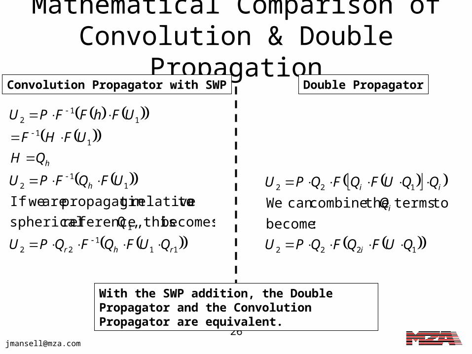
Mathematical Comparison of Convolution & Double
Propagation
111
22
r
11
2
11
11
2
:becomes this,Q reference, spherical
a torelative gpropagatin are weIf
rhr
h
h
QUFQFQPU
UFQFPU
QH
UFHF
UFhFFPU
1222
122
:become
toterms thecombinecan We
QUFQFQPU
Q
QQUFQFQPU
i
i
ii
Convolution Propagator with SWP Double Propagator
With the SWP addition, the Double Propagator and the Convolution Propagator are equivalent.
27
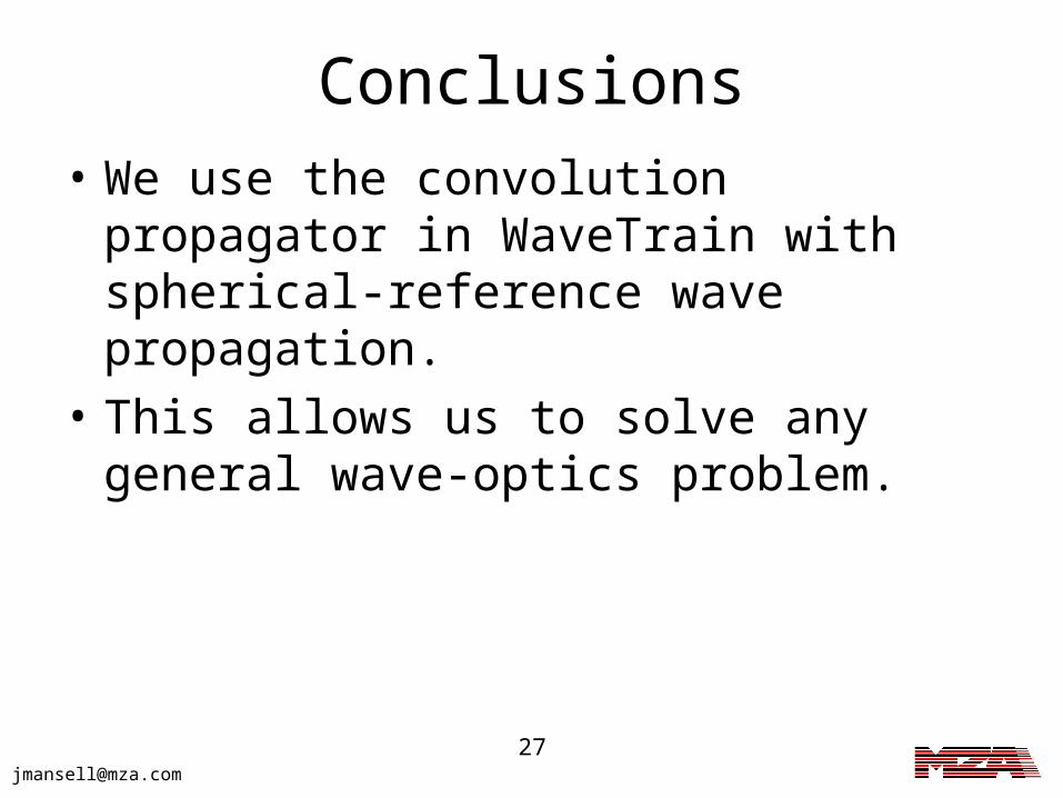
Conclusions• We use the convolution propagator in
WaveTrain with spherical-reference wave propagation.
• This allows us to solve any general wave-optics problem.
29
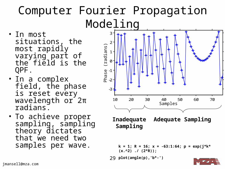
Computer Fourier Propagation Modeling
• In most situations, the most rapidly varying part of the field is the QPF.
• In a complex field, the phase is reset every wavelength or 2π radians.
• To achieve proper sampling, sampling theory dictates that we need two samples per wave.
10 20 30 40 50 60 70
-3
-2
-1
0
1
2
3
Adequate SamplingInadequateSampling
k = 1; R = 16; x = -63:1:64; p = exp(j*k* (x.^2) ./ (2*R));
plot(angle(p),'b*-')
SamplesP
hase
(ra
dian
s)
31
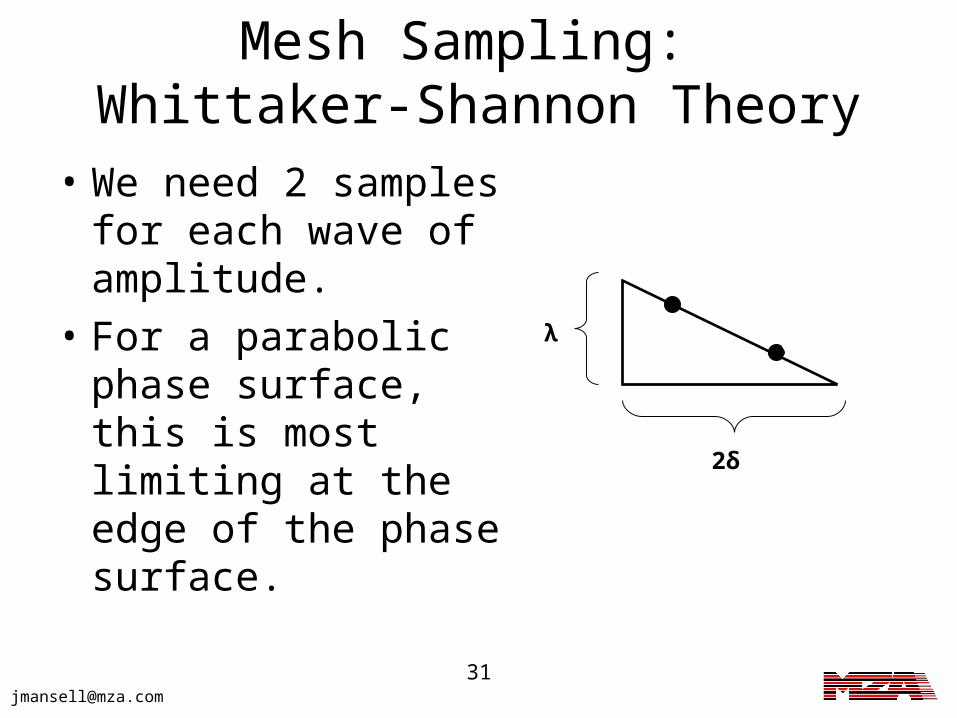
Mesh Sampling: Whittaker-Shannon Theory
• We need 2 samples for each wave of amplitude.
• For a parabolic phase surface, this is most limiting at the edge of the phase surface.
λ
2δ
32
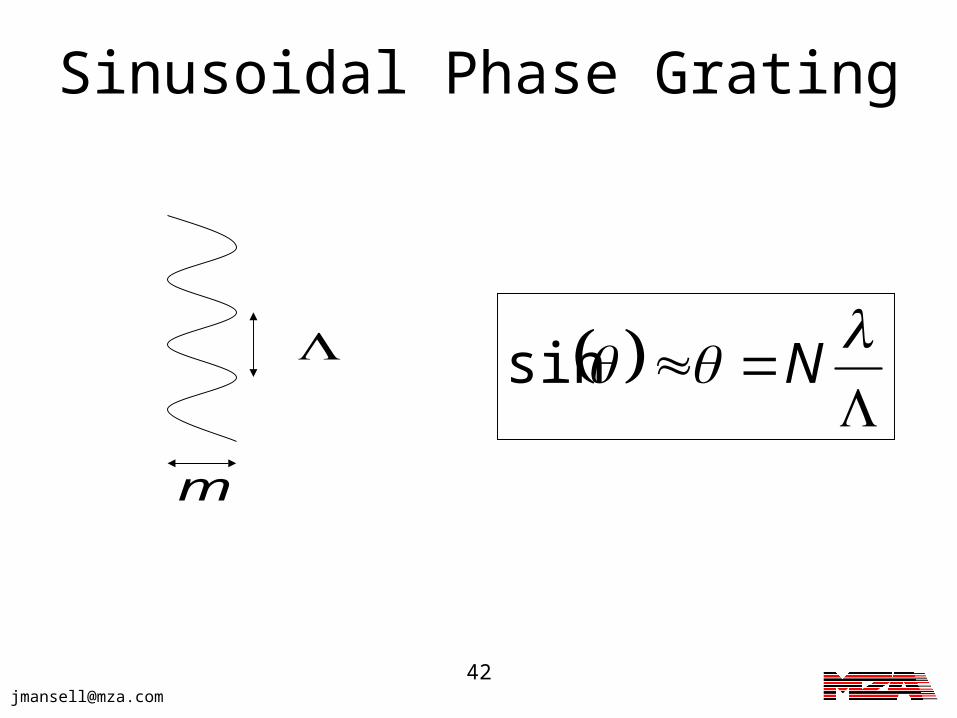
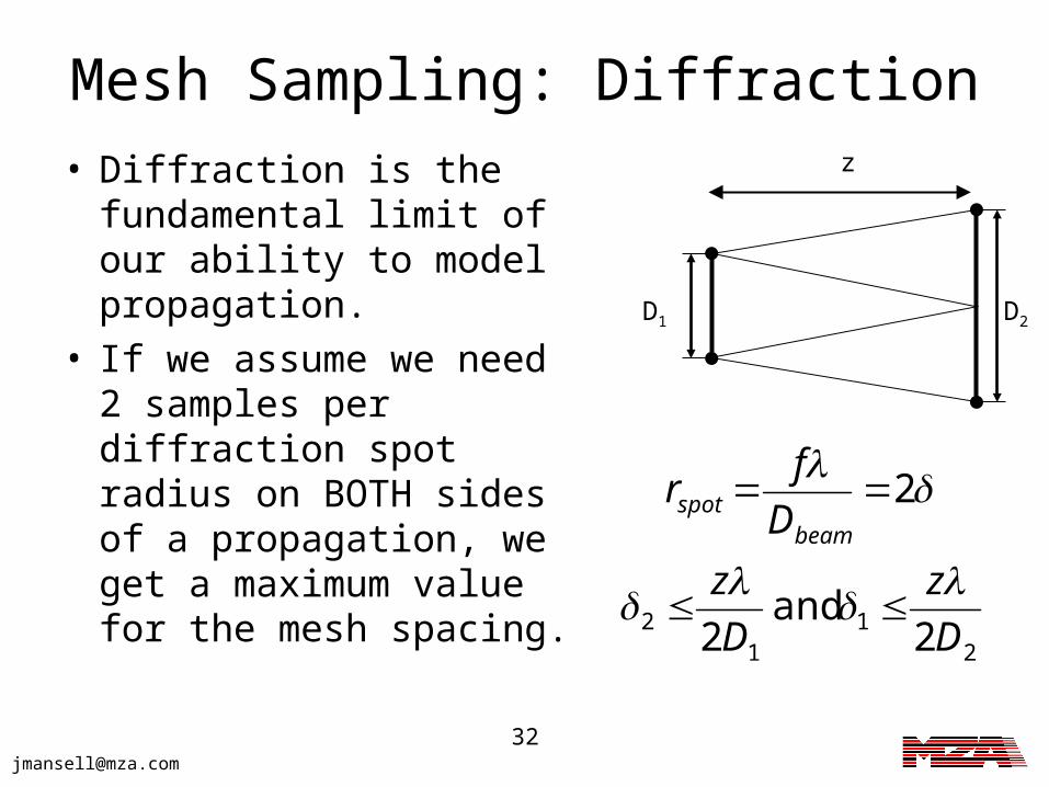
Mesh Sampling: Diffraction• Diffraction is the
fundamental limit of our ability to model propagation.
• If we assume we need 2 samples per diffraction spot radius on BOTH sides of a propagation, we get a maximum value for the mesh spacing.
z
21
12 2
and 2
2
D
z
D
z
D
fr
beamspot
D1 D2
33
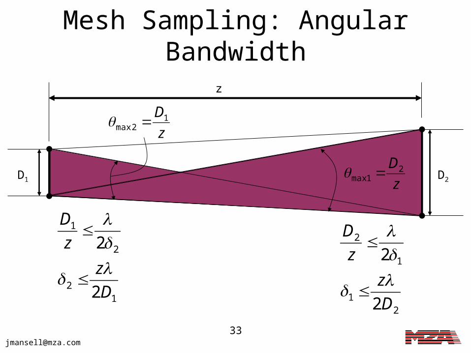
Mesh Sampling: Angular Bandwidth
D1 D2
z
z
D21max
21
1
2
2
2
D
z
z
D
z
D12max
12
2
1
2
2
D
z
z
D
34
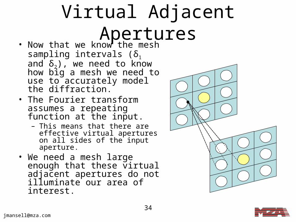
Virtual Adjacent Apertures• Now that we know the mesh
sampling intervals (δ1 and δ2), we need to know how big a mesh we need to use to accurately model the diffraction.
• The Fourier transform assumes a repeating function at the input.– This means that there are
effective virtual apertures on all sides of the input aperture.
• We need a mesh large enough that these virtual adjacent apertures do not illuminate our area of interest.
35
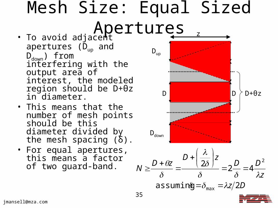
Mesh Size: Equal Sized Apertures
• To avoid adjacent apertures (Dup and Ddown) from interfering with the output area of interest, the modeled region should be D+θz in diameter.
• This means that the number of mesh points should be this diameter divided by the mesh spacing (δ).
• For equal apertures, this means a factor of two guard-band.
D+θzD D
z
Dup
Ddown
Dzz
DDzD
zDN
2 assuming
422
max
2
36
Unequal Apertures• For unequal apertures (such
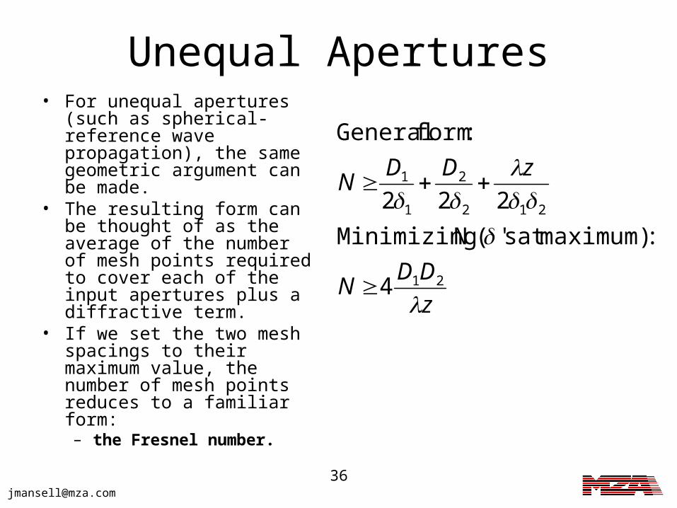
as spherical-reference wave propagation), the same geometric argument can be made.
• The resulting form can be thought of as the average of the number of mesh points required to cover each of the input apertures plus a diffractive term.
• If we set the two mesh spacings to their maximum value, the number of mesh points reduces to a familiar form: – the Fresnel number.
z
DDN
zDDN
21
212
2
1
1
4
:maximum)at s'( N Minimizing
222
:form General
37
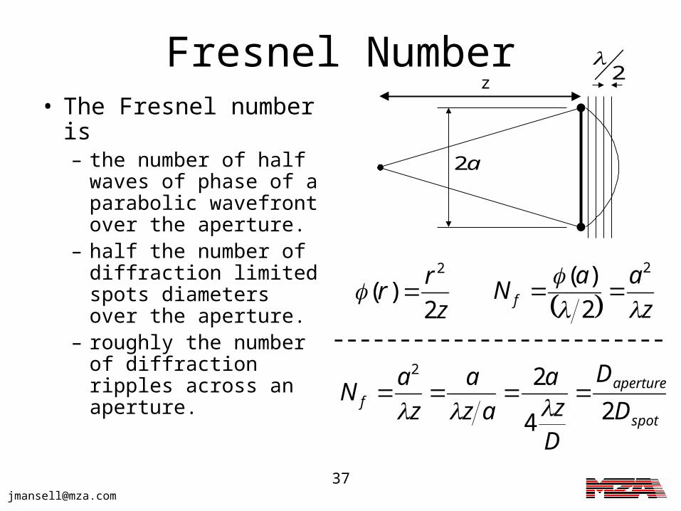
Fresnel Number• The Fresnel number
is – the number of half
waves of phase of a parabolic wavefront over the aperture.
– half the number of diffraction limited spots diameters over the aperture.
– roughly the number of diffraction ripples across an aperture.
z
rr
2)(
2
z
aaN f
2
2
)(
spot
aperturef D
D
Dz
a
az
a
z
aN
24
22
z
a2
2
38
Mesh Size and Fresnel Number
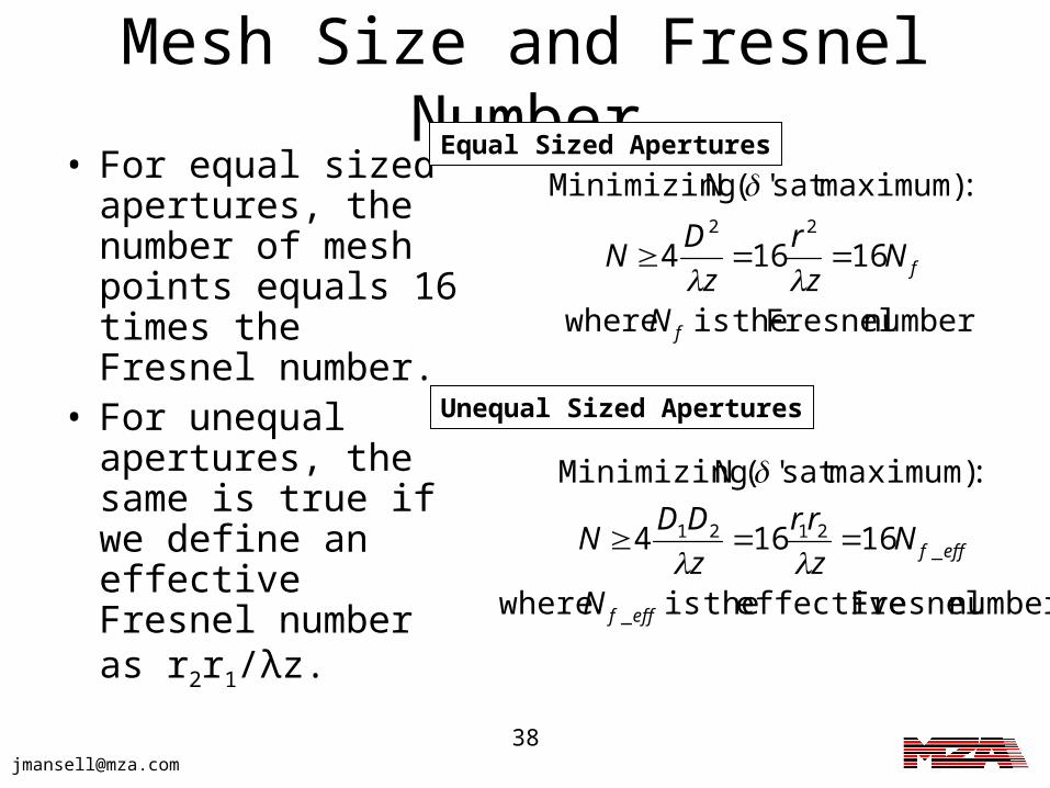
• For equal sized apertures, the number of mesh points equals 16 times the Fresnel number.
• For unequal apertures, the same is true if we define an effective Fresnel number as r2r1/λz.
number Fresnel theis where
16164
:maximum)at s'( N Minimizing22
f
f
N
Nz
r
z
DN
number Fresnel effective theis where
16164
:maximum)at s'( N Minimizing
_
_2121
efff
efff
N
Nz
rr
z
DDN
Equal Sized Apertures
Unequal Sized Apertures
39
Summary of Mesh Determination
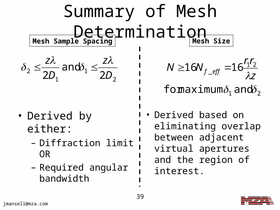
• Derived by either:– Diffraction limit OR– Required angular
bandwidth
• Derived based on eliminating overlap between adjacent virtual apertures and the region of interest.
Mesh Sample Spacing Mesh Size
21
12 2
and 2 D
z
D
z
21
21_
and maximumfor
1616
z
rrNN efff
40
Conclusions• For a simple system of two limiting
apertures, we have determined a set of inequalities that govern the choice of the mesh.
• Next we will look at – how phase aberrations impact the mesh
choice, and– how this can be extended to a system of
multiple apertures.
43
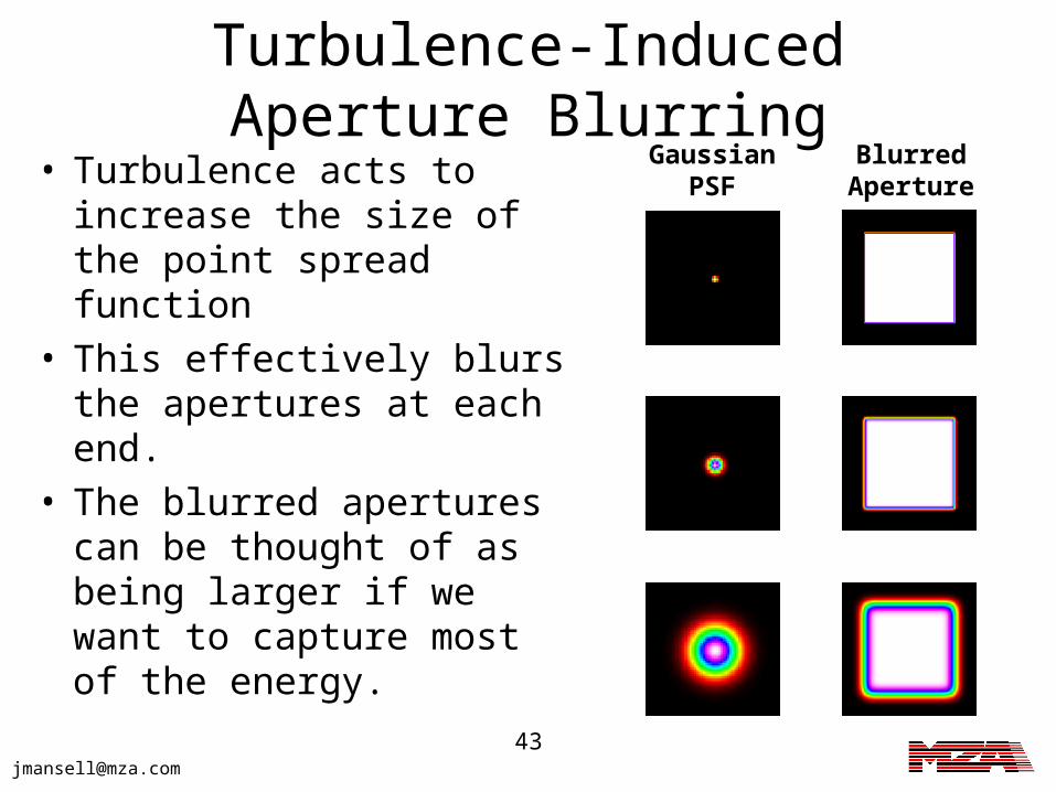
Turbulence-Induced Aperture Blurring
• Turbulence acts to increase the size of the point spread function
• This effectively blurs the apertures at each end.
• The blurred apertures can be thought of as being larger if we want to capture most of the energy.
GaussianPSF
BlurredAperture
44
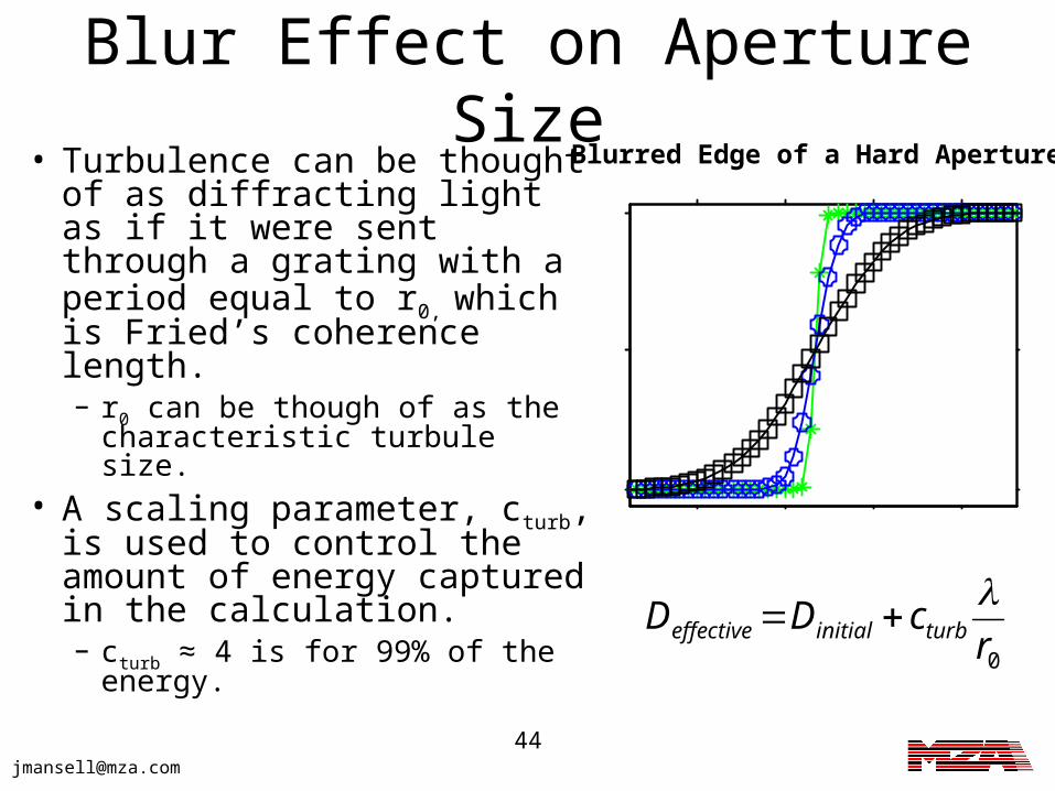
Blur Effect on Aperture Size• Turbulence can be thought
of as diffracting light as if it were sent through a grating with a period equal to r0, which is Fried’s coherence length.– r0 can be though of as the
characteristic turbule size.• A scaling parameter, cturb, is
used to control the amount of energy captured in the calculation.– cturb ≈ 4 is for 99% of the
energy.0r
cDD turbinitialeffective
180 190 200 210
0
0.5
1
Blurred Edge of a Hard Aperture
45
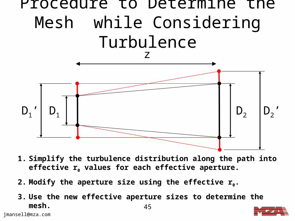
Procedure to Determine the Mesh while Considering
Turbulencez
D1 D2
1. Simplify the turbulence distribution along the path into effective r0 values for each effective aperture.
2. Modify the aperture size using the effective r0.
3. Use the new effective aperture sizes to determine the mesh.
D2’D1’
46
Determining Fourier Propagation Mesh
Parameters for Complex Optical Systems of Simple
Optics
47
Introduction• The determination of mesh parameters for
wave-optics modeling can be uniquely determined by a pair of limiting apertures separated by a finite distance.
• An optical system comprised of a set of ideal optics can be analyzed to determine the two limiting apertures that most restrict rays propagating through the system using field and aperture stop techniques.
48
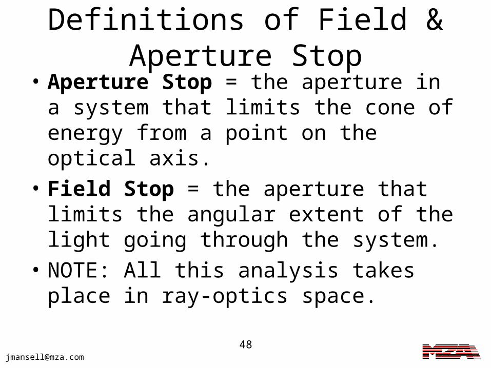
Definitions of Field & Aperture Stop
• Aperture Stop = the aperture in a system that limits the cone of energy from a point on the optical axis.
• Field Stop = the aperture that limits the angular extent of the light going through the system.
• NOTE: All this analysis takes place in ray-optics space.
49
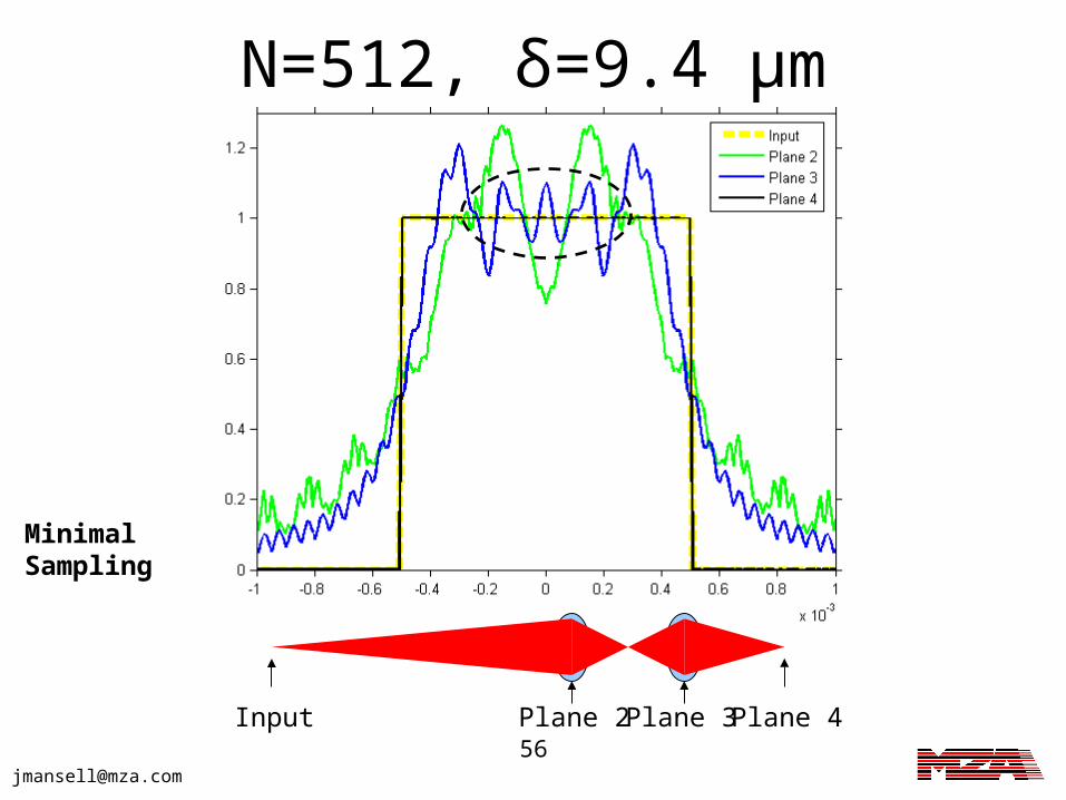
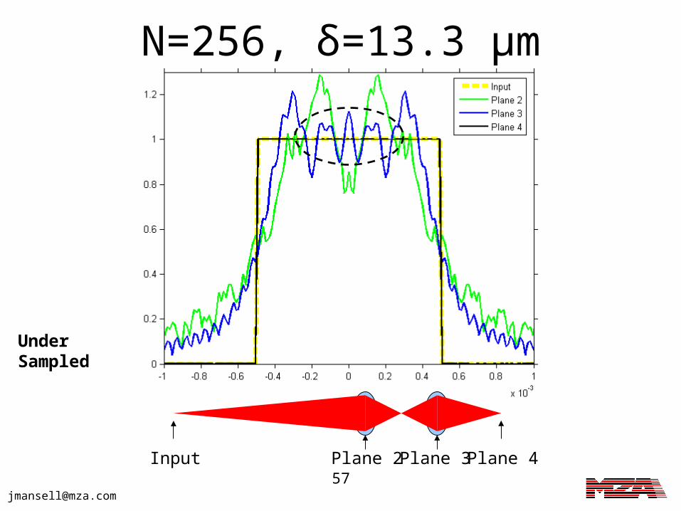
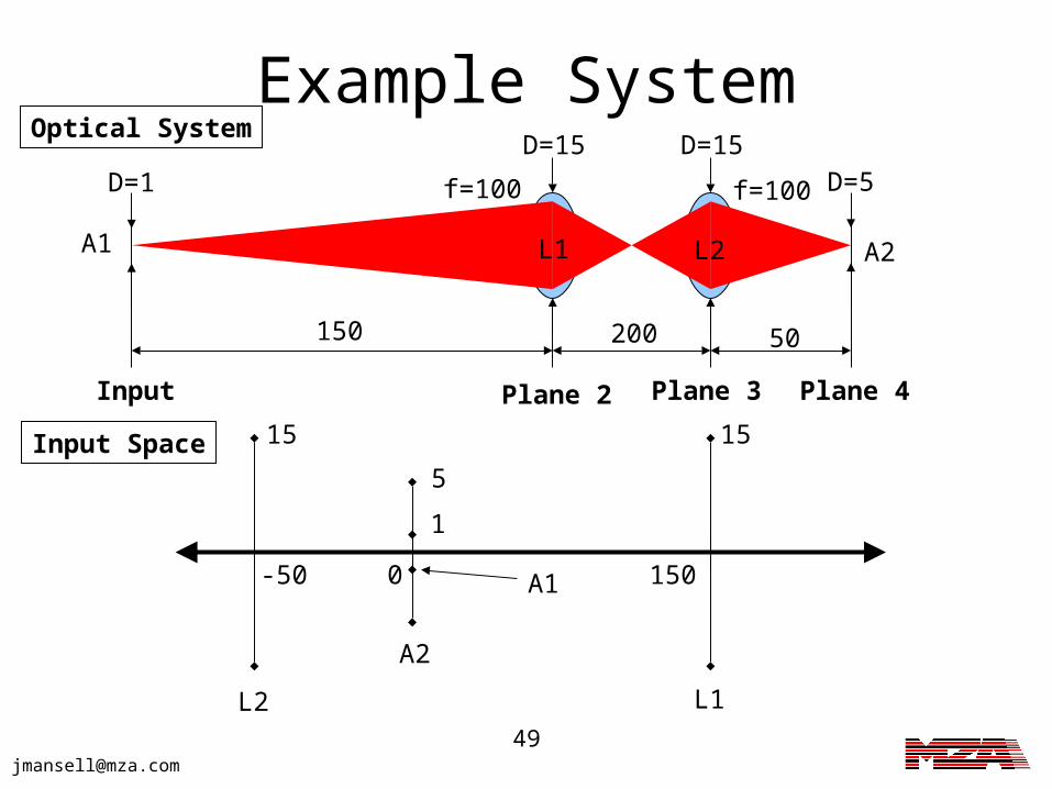
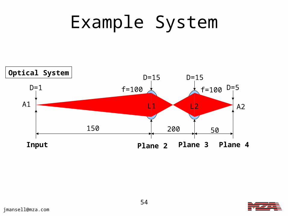
Example System
f=100 f=100
200150 50
D=15 D=15
D=5
L1 L2
-50 0 150
15 15
5
1
L2 L1
A2
A1
A2A1
D=1
Input Space
Optical System
Plane 2 Plane 3 Plane 4Input
50
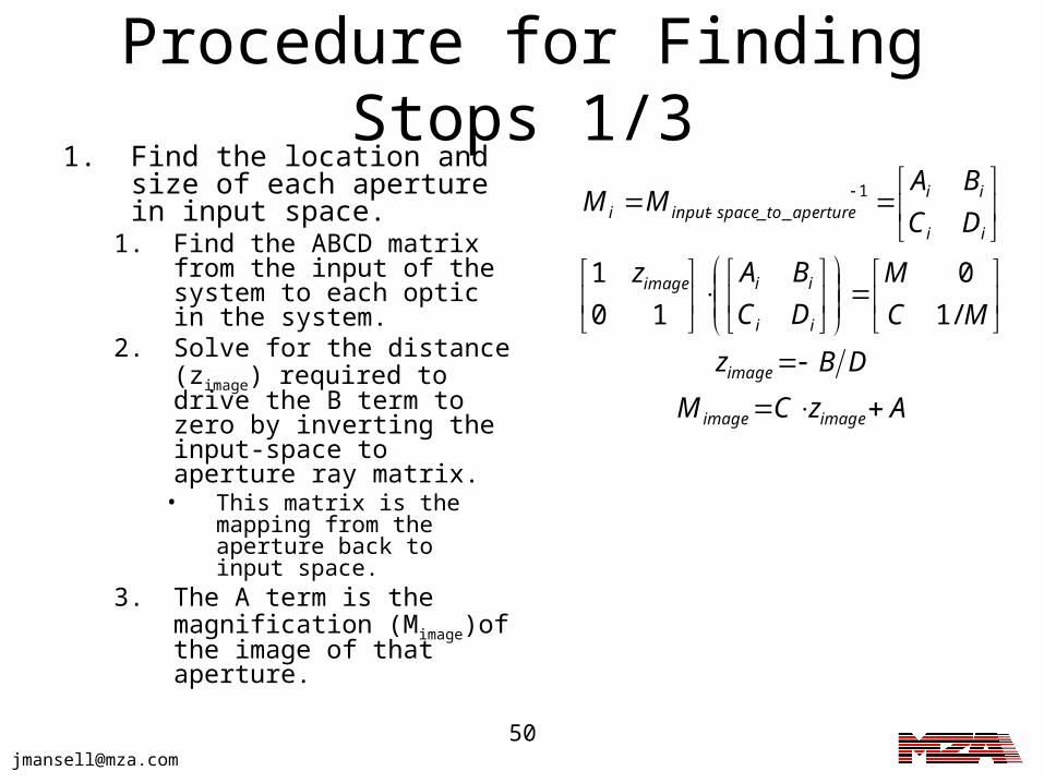
Procedure for Finding Stops 1/3
1. Find the location and size of each aperture in input space.
1. Find the ABCD matrix from the input of the system to each optic in the system.
2. Solve for the distance (zimage) required to drive the B term to zero by inverting the input-space to aperture ray matrix.
• This matrix is the mapping from the aperture back to input space.
3. The A term is the magnification (Mimage)of the image of that aperture.
AzCM
DBz
MC
M
DC
BAz
DC
BAMM
imageimage
image
ii
iiimage
ii
iiaperturetospaceinputi
/1
0
10
1
1__
51
Procedure for Finding Stops 2/3
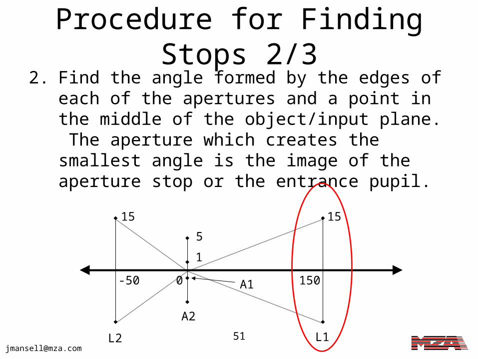
2. Find the angle formed by the edges of each of the apertures and a point in the middle of the object/input plane. The aperture which creates the smallest angle is the image of the aperture stop or the entrance pupil.
-50 0 150
15 15
5
1
L2 L1
A2
A1
52
Procedure for Finding Stops 3/3
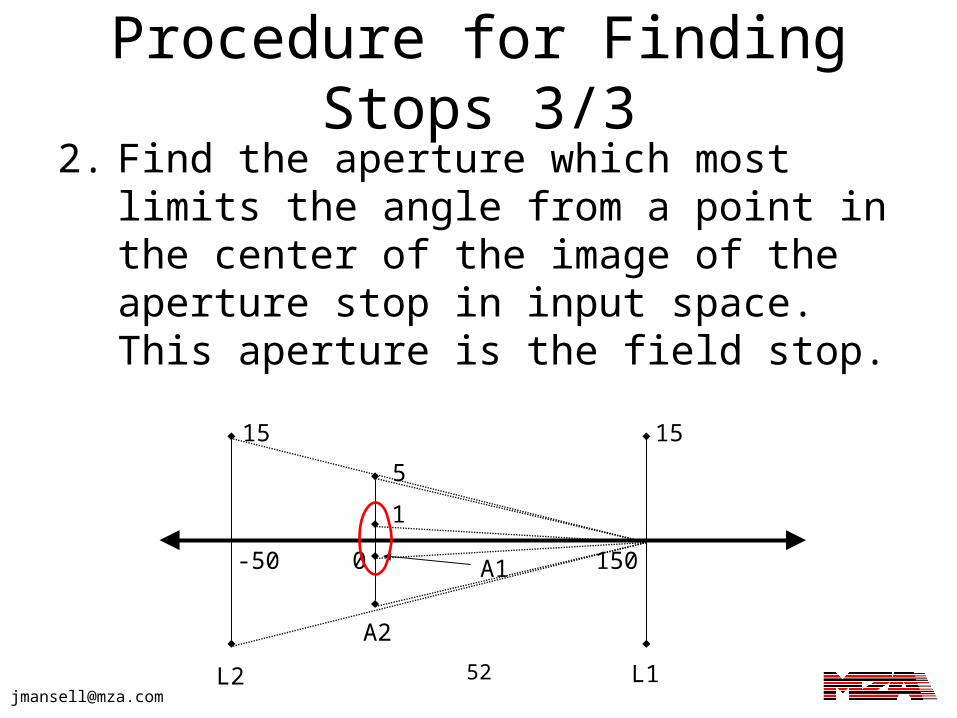
2. Find the aperture which most limits the angle from a point in the center of the image of the aperture stop in input space. This aperture is the field stop.
-50 0 150
15 15
5
1
L2 L1
A2
A1
53
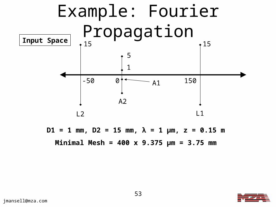
Example: Fourier Propagation
-50 0 150
15 15
5
1
L2 L1
A2
A1
Input Space
D1 = 1 mm, D2 = 15 mm, λ = 1 μm, z = 0.15 m
Minimal Mesh = 400 x 9.375 μm = 3.75 mm
54
Example System
f=100 f=100
200150 50
D=15 D=15
D=5
L1 L2 A2A1
D=1
Optical System
Plane 2 Plane 3 Plane 4Input
58
Conclusions of Complex System Mesh Parameter
Determination• We have devised a procedure to reduce a
complex system comprised of simple optics into a pair of the most restricting apertures.
• It would be nice to have a way of simplifying a complex system of simple optics so that modeling it is computationally easier…
60
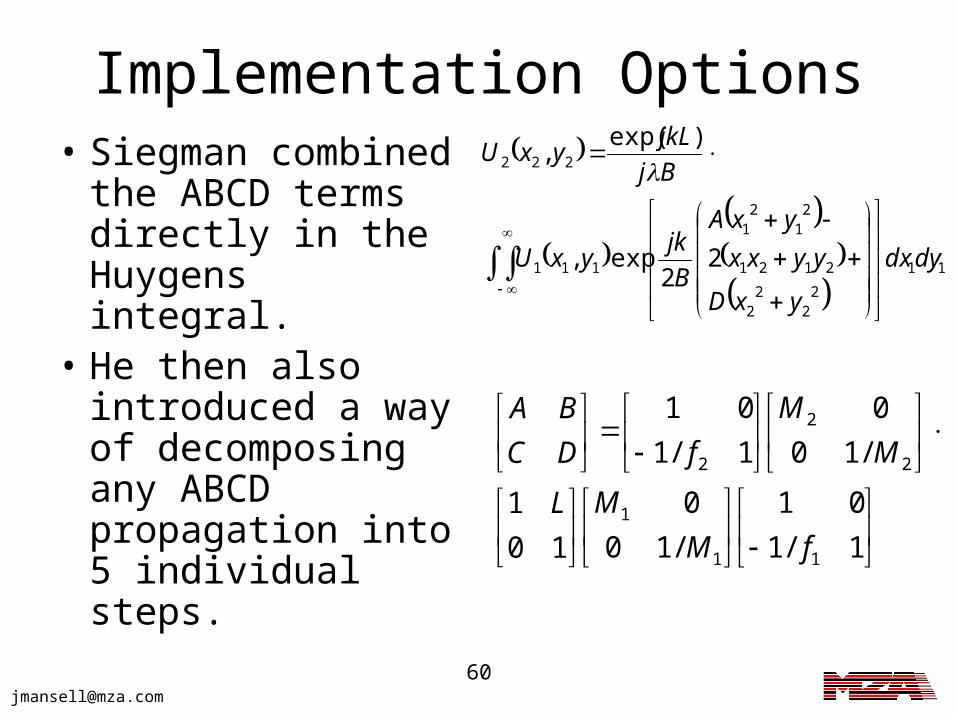
Implementation Options• Siegman combined
the ABCD terms directly in the Huygens integral.
• He then also introduced a way of decomposing any ABCD propagation into 5 individual steps.
11
22
22
2121
21
21
111
222
22
exp,
)exp(,
dydx
yxD
yyxx
yxA
B
jkyxU
Bj
jkLyxU
1/1
01
/10
0
10
1
/10
0
1/1
01
11
1
2
2
2
fM
ML
M
M
fDC
BA
61
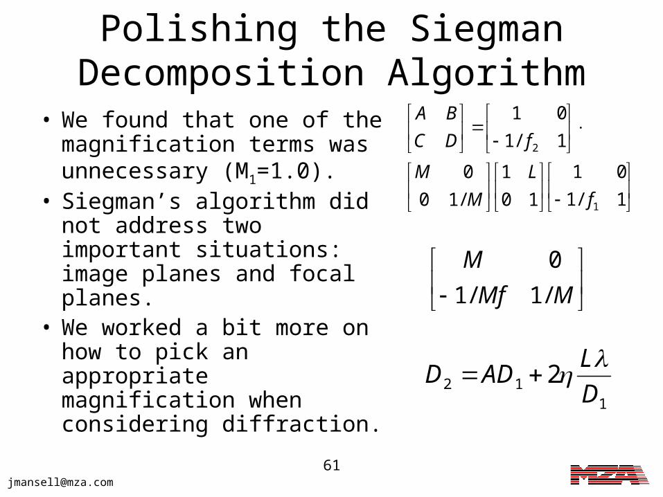
Polishing the Siegman Decomposition Algorithm
• We found that one of the magnification terms was unnecessary (M1=1.0).
• Siegman’s algorithm did not address two important situations: image planes and focal planes.
• We worked a bit more on how to pick an appropriate magnification when considering diffraction.
1/1
01
10
1
/10
0
1/1
01
1
2
f
L
M
M
fDC
BA
MMf
M
/1/1
0
112 2
D
LADD
62
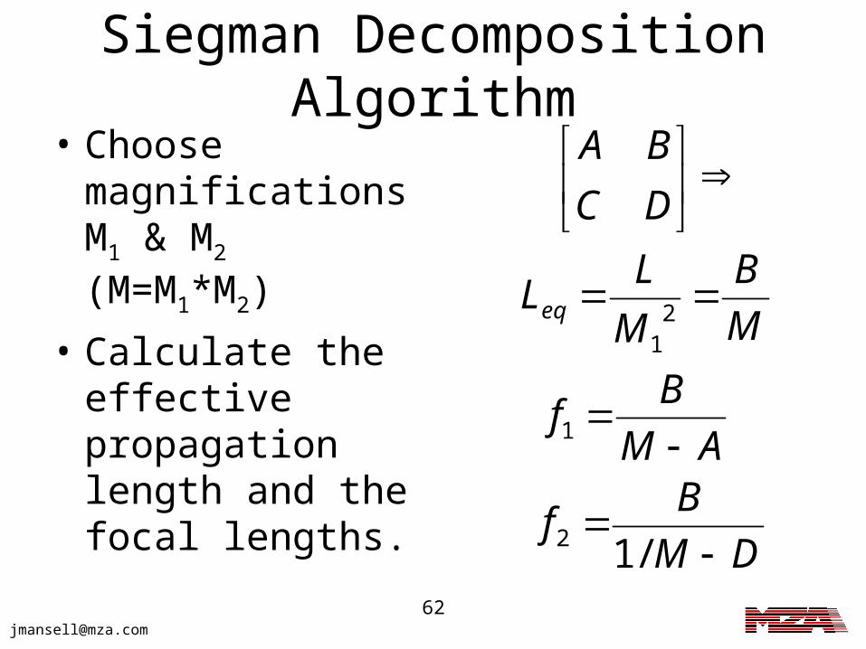
Siegman Decomposition Algorithm
• Choose magnifications M1 & M2 (M=M1*M2)
• Calculate the effective propagation length and the focal lengths.
DM
Bf
AM
Bf
M
B
M
LL
DC
BA
eq
/1
2
1
21
63
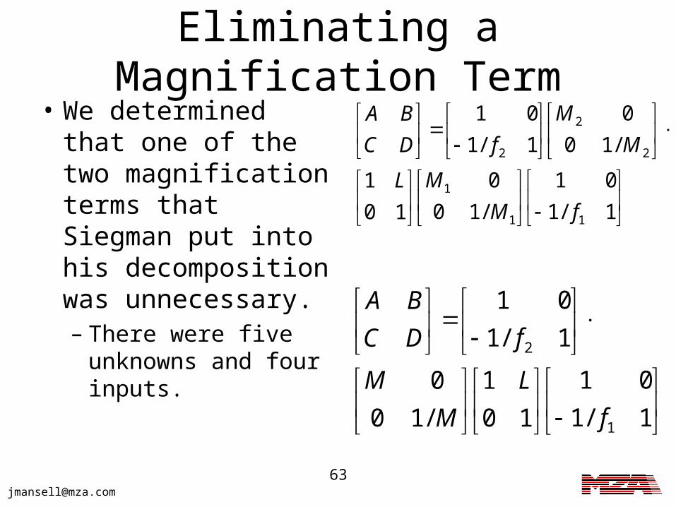
Eliminating a Magnification Term
• We determined that one of the two magnification terms that Siegman put into his decomposition was unnecessary.– There were five
unknowns and four inputs.
1/1
01
10
1
/10
0
1/1
01
1
2
f
L
M
M
fDC
BA
1/1
01
/10
0
10
1
/10
0
1/1
01
11
1
2
2
2
fM
ML
M
M
fDC
BA
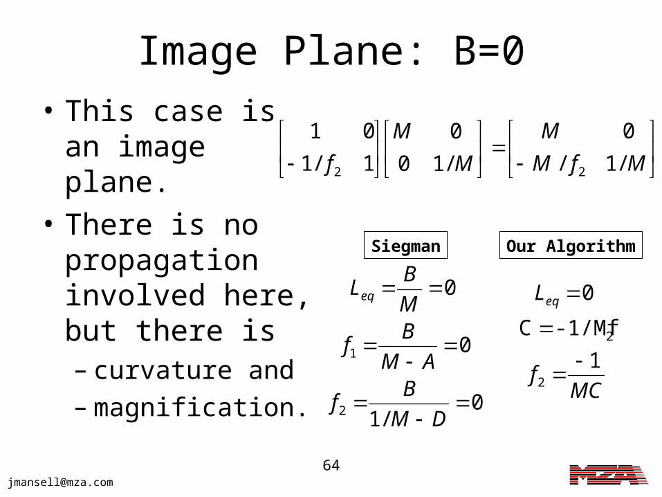
64
Image Plane: B=0• This case is an
image plane.
• There is no propagation involved here, but there is – curvature and– magnification.
MfM
M
M
M
f /1/
0
/10
0
1/1
01
22
0/1
0
0
2
1
DM
Bf
AM
Bf
M
BLeq
MCf
Leq
1
-1/MfC
0
2
2
Siegman Our Algorithm
65
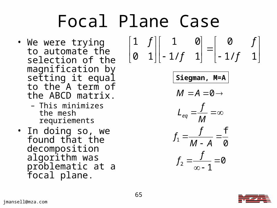
Focal Plane Case• We were trying to
automate the selection of the magnification by setting it equal to the A term of the ABCD matrix.– This minimizes the
mesh requriements• In doing so, we found
that the decomposition algorithm was problematic at a focal plane.
01
0
f
0
2
1
ff
AM
ff
M
fL
AM
eq
Siegman, M=A
1/1
0
1/1
01
10
1
f
f
f
f
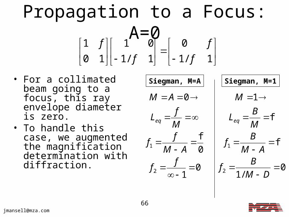
66
Propagation to a Focus: A=0
1/1
0
1/1
01
10
1
f
f
f
f
0/1
f
f
1
2
1
DM
Bf
AM
Bf
M
BL
M
eq
Siegman, M=1
01
0
f
0
2
1
ff
AM
ff
M
fL
AM
eq
Siegman, M=A• For a collimated beam going to a focus, this ray envelope diameter is zero.
• To handle this case, we augmented the magnification determination with diffraction.
67
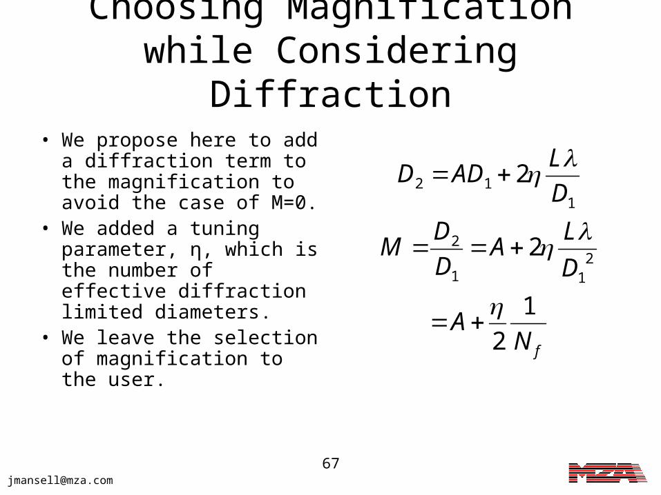
Choosing Magnification while Considering Diffraction
fNA
D
LA
D
DM
D
LADD
1
2
2
2
211
2
112
• We propose here to add a
diffraction term to the magnification to avoid the case of M=0.
• We added a tuning parameter, η, which is the number of effective diffraction limited diameters.
• We leave the selection of magnification to the user.
68
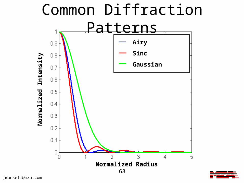
Common Diffraction Patterns
Airy
Sinc
Gaussian
No
rmal
ized
In
ten
sity
Normalized Radius
69
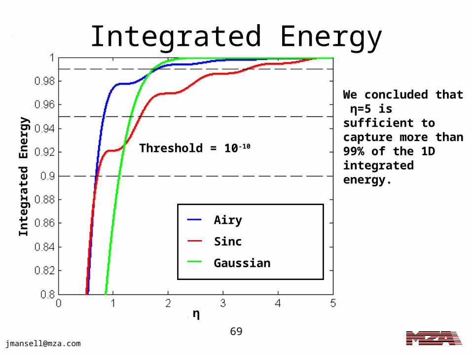
Integrated Energy
Threshold = 10-10
Airy
Sinc
Gaussian
Inte
gra
ted
En
erg
y
η
We concluded that η=5 is sufficient to capture more than 99% of the 1D integrated energy.
70
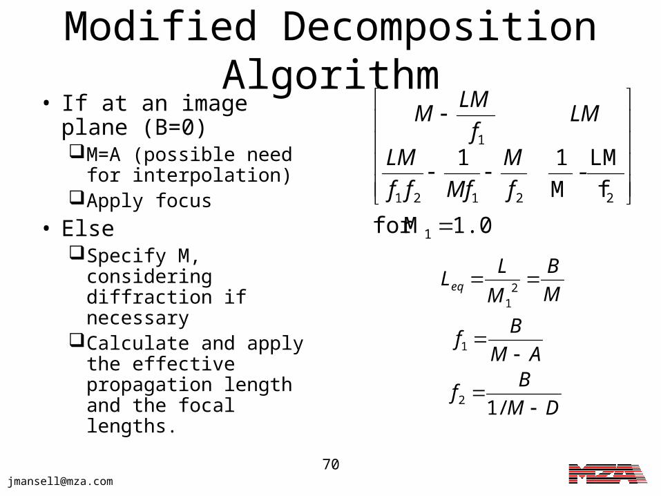
Modified Decomposition Algorithm
• If at an image plane (B=0)M=A (possible need for
interpolation)Apply focus
• ElseSpecify M, considering
diffraction if necessaryCalculate and apply the
effective propagation length and the focal lengths. DM
Bf
AM
Bf
M
B
M
LLeq
/1
2
1
21
1.0Mfor
f
LM-
M
11
1
22121
1
f
M
Mfff
LM
LMf
LMM
71
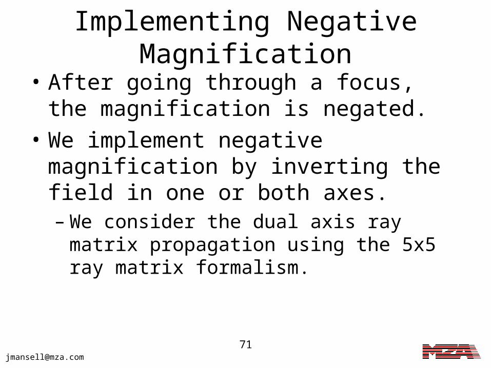
Implementing Negative Magnification
• After going through a focus, the magnification is negated.
• We implement negative magnification by inverting the field in one or both axes. – We consider the dual axis ray matrix
propagation using the 5x5 ray matrix formalism.

72
Dual Axis Implementation• In our
implementation, we handle the case of cylindrical telescopes along the axes by dividing the convolution kernel into separate parts for the two axes.
22
11
2
exp yyxx fzfzjH
UFHFPU
77
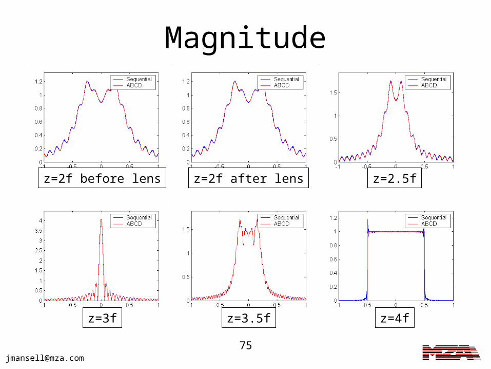
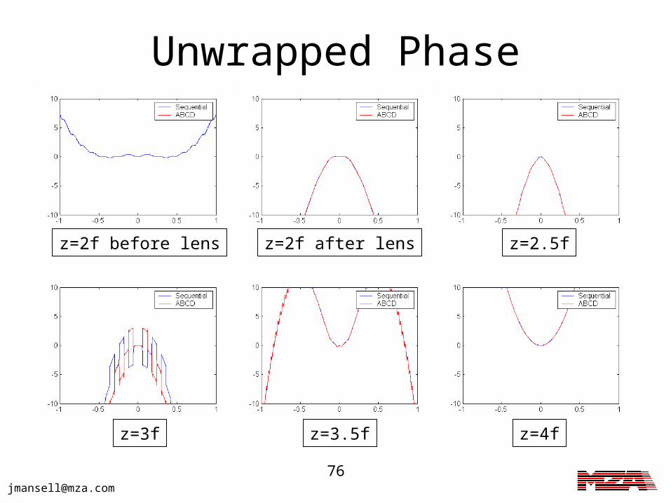
ABCD Ray Matrix Fourier PropagationConclusions
• We have modified Siegman’s ABCD decomposition algorithm to include several special cases, including:– Image planes– Propagation to a focus
• This enables complex systems comprised of simple optical elements to be modeled in 4 steps.