Embed Size (px)
Citation preview

Downside Risk
Louis ScottKiema Advisors
Northfield London Conference, November 2012
Downside Risk 1 / 53
1 Introduction
2 Methods and Data
3 Downside Risk
4 Asset Pricing Design
5 Asset Pricing Results
6 Conclusion
Downside Risk Outline 2 / 53
Motivation
I Bearers of downside risk should earn a reward for holding assetsthat under-perform in bad markets when the preservation of wealthis paramount.
I Demonstrate a tradable, simple to build proxy.I Questions:
I Going back to the 1950’s to the present, does it work as advertised?I Is there evidence from an asset pricing framework?
Downside Risk Introduction 3 / 53
Motivation
I Bearers of downside risk should earn a reward for holding assetsthat under-perform in bad markets when the preservation of wealthis paramount.
I Demonstrate a tradable, simple to build proxy.
I Questions:
I Going back to the 1950’s to the present, does it work as advertised?I Is there evidence from an asset pricing framework?
Downside Risk Introduction 3 / 53
Motivation
I Bearers of downside risk should earn a reward for holding assetsthat under-perform in bad markets when the preservation of wealthis paramount.
I Demonstrate a tradable, simple to build proxy.I Questions:
I Going back to the 1950’s to the present, does it work as advertised?
I Is there evidence from an asset pricing framework?
Downside Risk Introduction 3 / 53
Motivation
I Bearers of downside risk should earn a reward for holding assetsthat under-perform in bad markets when the preservation of wealthis paramount.
I Demonstrate a tradable, simple to build proxy.I Questions:
I Going back to the 1950’s to the present, does it work as advertised?I Is there evidence from an asset pricing framework?
Downside Risk Introduction 3 / 53
Background
The Literature
Relating stock level returns to return asymmetry.
I Beta asymmetry: Bawa & Lindenberg (1977), Ang, Chen & Xing(2005) find that stocks which co-vary strongly with the market whenthe market declines have high average returns and that the downsiderisk premium is approximately 6% per annum. Ex-post construction.
I Higher moments: Harvey and Siddique 2000, Bakshi, Kapadiaand Madan 2003 and Conrad Dittmar and Ghysels 2008 find thatmore negatively (positively) skewed returns associated withsubsequent higher (lower) returns.
I Tail measures Bali, Demirtas & Levy (2009) show that VaRdominates expected shortfall and tail risk and on average predictsreturns positively.
I Survey of the Literature See DiBartolomeo 2007 for a survey ofthe literature on higher order moments, and their implications forasset pricing models.
Downside Risk Introduction 4 / 53

The Data
I The data, the HML, SMB and WML portfolios are from KenFrench’s website. We also downloaded the 10 decile portfolios forBook, Size, Mom and the 38 industry portfolios. The industryportfolios are then reduced to 34 after deleting industries withmissing data. Macro data is from the FRED website.
I This paper is most closely tied to Bawa & Lindenberg (1977), andAng, Chen & Xing 2005. Unlike Ang, whose measure is an ex-postbeta measure, the aim is to construct a trade-able portfolio thatearns the aforementioned premium.
Downside Risk Methods and Data 5 / 53

Downside Risk Motivation
The intuition
Macroeconomic news impacts industries differently.
I Conover, Jensen, Johnson & Mercer (2008) that there arestrong monetary policy effects across sectors.
I Moskowitz & Grinblatt (1999) find that the profitability of amomentum strategy is primarily attributable to industry levelmomentum.
I Chordia & Shivakumar (2000) find that the profits can beexplained by loadings to lagged macroeconomic variables. In ourmeasure, we posit that downside risk exposure proxies for theincreased risks associated with the macro driven component toindustry returns.
Downside Risk Methods and Data 6 / 53
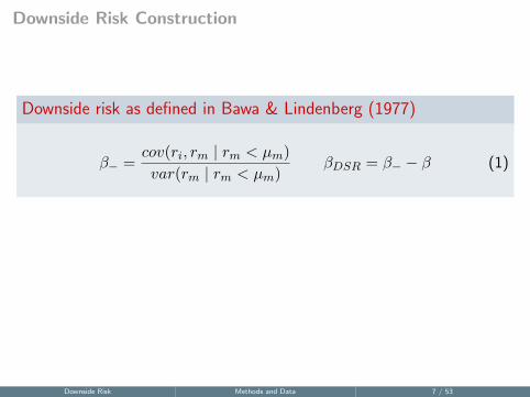
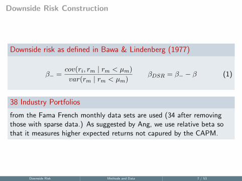
Downside Risk Construction
Downside risk as defined in Bawa & Lindenberg (1977)
β− =cov(ri, rm | rm < µm)
var(rm | rm < µm)βDSR = β− − β (1)
38 Industry Portfolios
from the Fama French monthly data sets are used (34 after removingthose with sparse data.) As suggested by Ang, we use relative beta sothat it measures higher expected returns not capured by the CAPM.
Downside Risk Methods and Data 7 / 53

Downside Risk Construction
Estimation window
Where Ang et al. use one year of daily data over a forward lookingperiod to construct their measure, we use the most recent two years ofmonthly history. The split then occurs for the months with marketreturns less than the two year mean.
Historical window
extends back to the mid 1950’s. The choice is to include only data afterT-bills were allowed to vary freely subsequent to the Federal ReserveAccord of 1951, and to include the 1962-2001 period used by Ang, Chenand Xing.
Downside Risk Methods and Data 8 / 53

Downside Risk
Figure: Downside Risk Quintile Portfolios.
Downside Risk Downside Risk 9 / 53
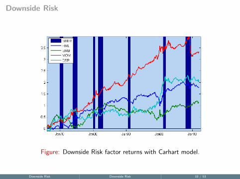
Downside Risk
Figure: Downside Risk factor returns with Carhart model.
Downside Risk Downside Risk 10 / 53
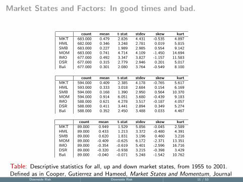
Market States and Factors: In good times and bad.
count mean t-stat stdev skew kurtMKT 683.000 0.479 2.826 4.431 -0.535 4.897HML 682.000 0.346 3.248 2.781 0.019 5.815SMB 683.000 0.227 1.989 2.985 0.554 9.142MOM 683.000 0.741 4.714 4.109 -1.450 14.694IMO 677.000 0.492 3.347 3.827 -1.157 11.583DSR 677.000 0.315 2.779 2.946 0.201 5.017Bali 677.000 0.301 2.080 3.764 -0.549 8.100
count mean t-stat stdev skew kurtMKT 594.000 0.409 2.385 4.178 -0.765 5.617HML 593.000 0.333 3.018 2.684 0.154 6.169SMB 594.000 0.168 1.390 2.950 0.564 10.370MOM 594.000 0.914 6.051 3.680 -0.439 9.183IMO 588.000 0.621 4.278 3.517 -0.187 4.057DSR 588.000 0.411 3.441 2.894 0.349 5.274Bali 588.000 0.352 2.450 3.488 0.033 4.467
count mean t-stat stdev skew kurtMKT 89.000 0.949 1.529 5.856 -0.045 2.589HML 89.000 0.433 1.213 3.372 -0.480 4.391SMB 89.000 0.620 1.831 3.196 0.460 3.216MOM 89.000 -0.409 -0.625 6.172 -2.371 13.351IMO 89.000 -0.354 -0.619 5.401 -2.596 16.716DSR 89.000 -0.320 -0.938 3.215 -0.398 3.429Bali 89.000 -0.040 -0.071 5.248 -1.542 10.762
Table: Descriptive statistics for all, up and down market states, from 1955 to 2001.Defined as in Cooper, Gutierrez and Hameed, Market States and Momentum, Journalof Finance, 2005Downside Risk Downside Risk 11 / 53

Market States and Factors: In good times and bad.
count mean t-stat stdev skew kurtMKT 683.000 0.479 2.826 4.431 -0.535 4.897HML 682.000 0.346 3.248 2.781 0.019 5.815SMB 683.000 0.227 1.989 2.985 0.554 9.142MOM 683.000 0.741 4.714 4.109 -1.450 14.694IMO 677.000 0.492 3.347 3.827 -1.157 11.583DSR 677.000 0.315 2.779 2.946 0.201 5.017Bali 677.000 0.301 2.080 3.764 -0.549 8.100
Table: Descriptive statistics for all months, from 1955 to 2001. Defined as inCooper, Gutierrez and Hameed, Market States and Momentum, Journal ofFinance, 2005
Downside Risk Downside Risk 12 / 53
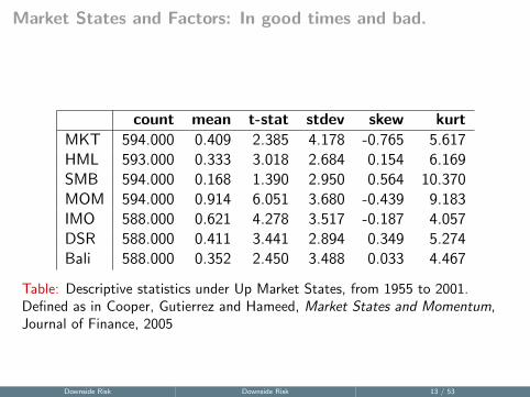
Market States and Factors: In good times and bad.
count mean t-stat stdev skew kurtMKT 594.000 0.409 2.385 4.178 -0.765 5.617HML 593.000 0.333 3.018 2.684 0.154 6.169SMB 594.000 0.168 1.390 2.950 0.564 10.370MOM 594.000 0.914 6.051 3.680 -0.439 9.183IMO 588.000 0.621 4.278 3.517 -0.187 4.057DSR 588.000 0.411 3.441 2.894 0.349 5.274Bali 588.000 0.352 2.450 3.488 0.033 4.467
Table: Descriptive statistics under Up Market States, from 1955 to 2001.Defined as in Cooper, Gutierrez and Hameed, Market States and Momentum,Journal of Finance, 2005
Downside Risk Downside Risk 13 / 53
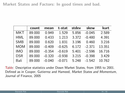
Market States and Factors: In good times and bad.
count mean t-stat stdev skew kurtMKT 89.000 0.949 1.529 5.856 -0.045 2.589HML 89.000 0.433 1.213 3.372 -0.480 4.391SMB 89.000 0.620 1.831 3.196 0.460 3.216MOM 89.000 -0.409 -0.625 6.172 -2.371 13.351IMO 89.000 -0.354 -0.619 5.401 -2.596 16.716DSR 89.000 -0.320 -0.938 3.215 -0.398 3.429Bali 89.000 -0.040 -0.071 5.248 -1.542 10.762
Table: Descriptive statistics under Down Market States, from 1955 to 2001.Defined as in Cooper, Gutierrez and Hameed, Market States and Momentum,Journal of Finance, 2005
Downside Risk Downside Risk 14 / 53
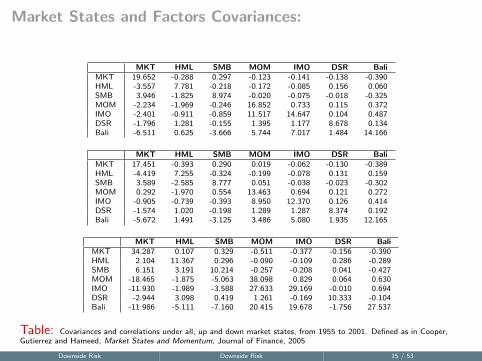
Market States and Factors Covariances:
MKT HML SMB MOM IMO DSR BaliMKT 19.652 -0.288 0.297 -0.123 -0.141 -0.138 -0.390HML -3.557 7.781 -0.218 -0.172 -0.085 0.156 0.060SMB 3.946 -1.825 8.974 -0.020 -0.075 -0.018 -0.325MOM -2.234 -1.969 -0.246 16.852 0.733 0.115 0.372IMO -2.401 -0.911 -0.859 11.517 14.647 0.104 0.487DSR -1.796 1.281 -0.155 1.395 1.177 8.678 0.134Bali -6.511 0.625 -3.666 5.744 7.017 1.484 14.166
MKT HML SMB MOM IMO DSR BaliMKT 17.451 -0.393 0.290 0.019 -0.062 -0.130 -0.389HML -4.419 7.255 -0.324 -0.199 -0.078 0.131 0.159SMB 3.589 -2.585 8.777 0.051 -0.038 -0.023 -0.302MOM 0.292 -1.970 0.554 13.463 0.694 0.121 0.272IMO -0.905 -0.739 -0.393 8.950 12.370 0.126 0.414DSR -1.574 1.020 -0.198 1.289 1.287 8.374 0.192Bali -5.672 1.491 -3.125 3.486 5.080 1.935 12.165
MKT HML SMB MOM IMO DSR BaliMKT 34.287 0.107 0.329 -0.511 -0.377 -0.156 -0.390HML 2.104 11.367 0.296 -0.090 -0.109 0.286 -0.289SMB 6.151 3.191 10.214 -0.257 -0.208 0.041 -0.427MOM -18.465 -1.875 -5.063 38.098 0.829 0.064 0.630IMO -11.930 -1.989 -3.588 27.633 29.169 -0.010 0.694DSR -2.944 3.098 0.419 1.261 -0.169 10.333 -0.104Bali -11.986 -5.111 -7.160 20.415 19.678 -1.756 27.537
Table: Covariances and correlations under all, up and down market states, from 1955 to 2001. Defined as in Cooper,Gutierrez and Hameed, Market States and Momentum, Journal of Finance, 2005
Downside Risk Downside Risk 15 / 53
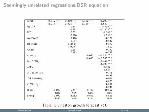
Seemingly unrelated regressions:DSR equation
const 0.312∗∗∗ 0.310∗∗∗ 0.312∗∗∗ 0.299∗∗∗
2.716∗∗∗ 2.825∗∗∗ 2.720∗∗∗ 2.840∗∗∗
lagLGR -0.147 −0.339∗∗
-1.211 −2.325∗∗
DY -0.031 0.307∗
-0.216 1.716∗
AVE3to10 0.126 -0.1290.647 -0.597
DIF3to10 0.384∗ 0.3791.929∗ 1.550
CRED -0.217 -0.199-0.983 -0.753
constS -0.090 −0.721∗∗∗
-0.430 −2.595∗∗∗
lagLGRS 0.452∗∗∗
3.020∗∗∗
DYS −0.592∗
−1.884∗
AV E3to10S 0.1730.498
DIF3to10S 0.0040.023
CREDS 0.2840.736
R-sqr 0.000 5.497 0.100 10.567NaN NaN NaN NaN
SysRq -0.000 3.962 0.843 8.857NaN NaN NaN NaN
Table: Livingston growth forecast < 0
Table: comments
Downside Risk Downside Risk 16 / 53
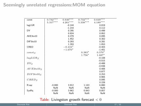
Seemingly unrelated regressions:MOM equation
const 0.732∗∗∗ 0.646∗∗∗ 0.732∗∗∗ 0.649∗∗∗
5.317∗∗∗ 4.261∗∗∗ 5.338∗∗∗ 4.189∗∗∗
lagLGR -0.144 0.019-1.233 0.112
DY 0.295 0.4990.924 0.952
AVE3to10 0.279 0.0951.452 0.302
DIF3to10 0.293 0.2811.293 1.053
CRED −0.416∗ -0.403−1.670∗ -1.451
constS 0.383∗ 0.570∗
1.756∗ 1.687∗
lagLGRS -0.108-0.515
DYS -0.488-0.938
AV E3to10S 0.4060.877
DIF3to10S 0.2530.965
CREDS 0.0950.228
R-sqr -0.000 3.912 1.143 6.880NaN NaN NaN NaN
SysRq -0.000 3.962 0.843 8.857NaN NaN NaN NaN
Table: Livingston growth forecast < 0
Table: comments
Downside Risk Downside Risk 17 / 53
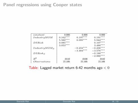
Panel regressions using Cooper states
constant 0.000 0.000 0.000IndustryMOM 0.162∗∗∗ 0.197∗∗∗ 0.191∗∗∗
5.560∗∗∗ 6.095∗∗∗ 5.944∗∗∗
DSRisk 0.085∗∗∗ 0.107∗∗∗
3.053∗∗∗ 3.488∗∗∗
IndustryMOMS −0.234∗∗∗ −0.236∗∗∗
−3.484∗∗∗ −3.576∗∗∗
DSRiskS −0.188∗∗∗
−2.886∗∗∗
R2 .0110 .0108 .0142Observations 22,185 22,185 22,185
Table: Lagged market return 6-42 months ago < 0
Downside Risk Downside Risk 18 / 53
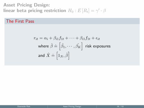
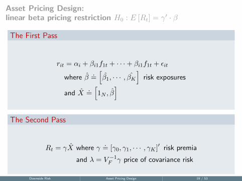
Asset Pricing Design:linear beta pricing restriction H0 : E [Rt] = γ′ · β
The First Pass
rit = αi + βi1f1t + · · ·+ βi1f1t + εit
where β̂.=[β̂1, · · · , β̂K
]risk exposures
and X̂.=[1N , β̂
]
The Second Pass
Rt = γX̂ where γ.= [γ0, γ1, · · · , γK ]′ risk premia
and λ = V −1F γ price of covariance risk
Downside Risk Asset Pricing Design 19 / 53
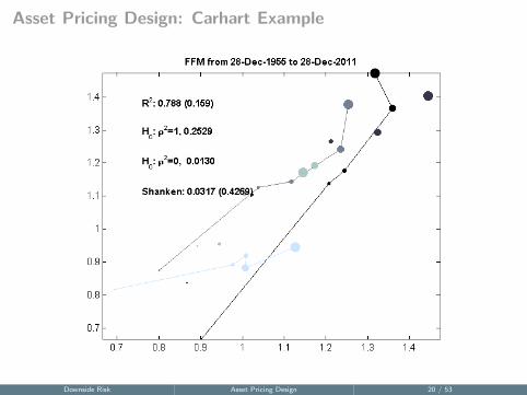
Asset Pricing Design: Carhart Example
Figure: CarhartDownside Risk Asset Pricing Design 20 / 53
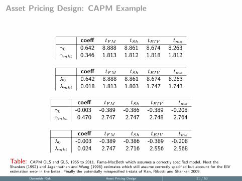
Asset Pricing Design: CAPM Example
coeff tFM tSh tEIV tms
γ0 0.642 8.888 8.861 8.674 8.263γmkt 0.346 1.813 1.812 1.818 1.812
coeff tFM tSh tEIV tms
λ0 0.642 8.888 8.861 8.674 8.263λmkt 0.018 1.813 1.803 1.747 1.743
coeff tFM tSh tEIV tms
γ0 -0.003 -0.389 -0.386 -0.389 -0.208γmkt 0.470 2.747 2.747 2.748 2.764
coeff tFM tSh tEIV tms
λ0 -0.003 -0.389 -0.386 -0.389 -0.208λmkt 0.024 2.747 2.716 2.556 2.568
Table: CAPM OLS and GLS, 1955 to 2011. Fama-MacBeth which assumes a correctly specified model. Next theShanken (1992) and Jagannathan and Wang (1998) estimates which still assume correctly specified but account for the EIVestimation error in the betas. Finally the potentially misspecified t-stats of Kan, Ribotti and Shanken 2009.
Downside Risk Asset Pricing Design 21 / 53
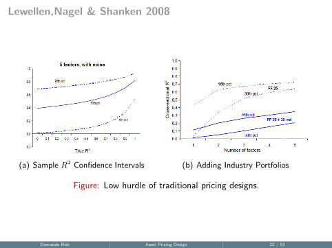
Lewellen,Nagel & Shanken 2008
(a) Sample R2 Confidence Intervals (b) Adding Industry Portfolios
Figure: Low hurdle of traditional pricing designs.
Downside Risk Asset Pricing Design 22 / 53
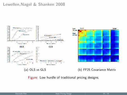
Lewellen,Nagel & Shanken 2008
(a) OLS vs GLS (b) FF25 Covariance Matrix
Figure: Low hurdle of traditional pricing designs.
Downside Risk Asset Pricing Design 23 / 53

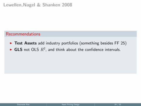
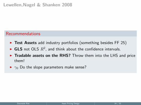
Lewellen,Nagel & Shanken 2008
Recommendations
I Test Assets add industry portfolios (something besides FF 25)
I GLS not OLS R2, and think about the confidence intervals.
I Tradable assets on the RHS? Throw them into the LHS and pricethem!
I γ0 Do the slope parameters make sense?
Downside Risk Asset Pricing Design 24 / 53
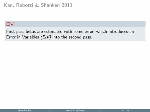
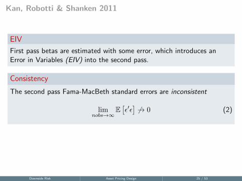
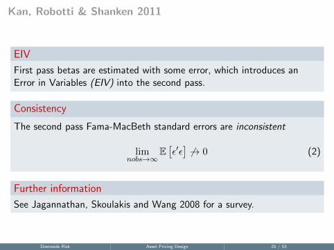
Kan, Robotti & Shanken 2011
EIV
First pass betas are estimated with some error, which introduces anError in Variables (EIV) into the second pass.
Consistency
The second pass Fama-MacBeth standard errors are inconsistent
limnobs→∞
E[ε′ε]6→ 0 (2)
Further information
See Jagannathan, Skoulakis and Wang 2008 for a survey.
Downside Risk Asset Pricing Design 25 / 53

Kan, Robotti & Shanken 2011
EIV
First pass betas are estimated with some error, which introduces anError in Variables (EIV) into the second pass.
Consistency
The second pass Fama-MacBeth standard errors are inconsistent
limnobs→∞
E[ε′ε]6→ 0 (3)
Futher information
See Jagannathan, Skoulakis and Wang 2008 for a survey.
Downside Risk Asset Pricing Design 26 / 53
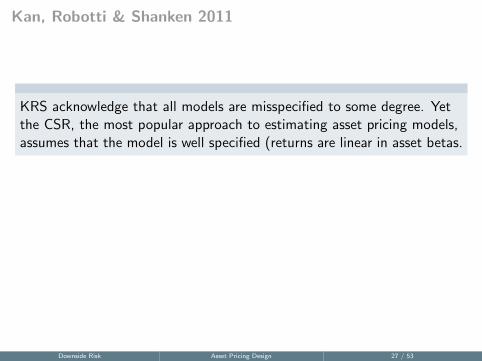
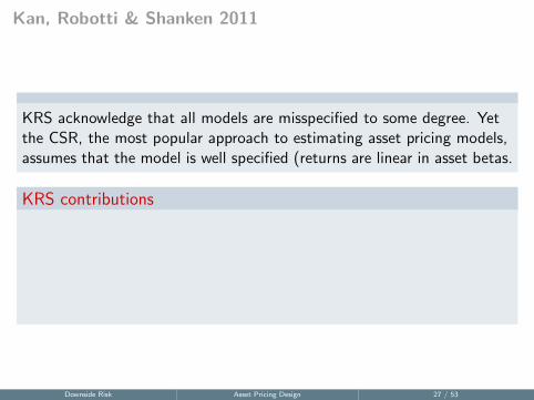
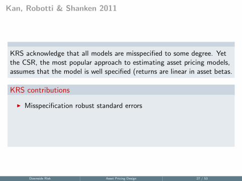
Kan, Robotti & Shanken 2011
KRS acknowledge that all models are misspecified to some degree. Yetthe CSR, the most popular approach to estimating asset pricing models,assumes that the model is well specified (returns are linear in asset betas.
KRS contributions
I Misspecification robust standard errors
I Derive the asymptotic distribution of the sample CSR R2
I Create a test for whether two pricing models have the samepopulation R2
Downside Risk Asset Pricing Design 27 / 53
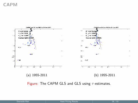
CAPM
(a) 1955-2011 (b) 1955-2011
Figure: The CAPM GLS and GLS using τ -estimates.
Downside Risk Asset Pricing Results 28 / 53

CAPM
coeff tFM tSh tEIV tms
γ0 0.642 8.888 8.861 8.674 8.263γmkt 0.346 1.813 1.812 1.818 1.812
coeff tFM tSh tEIV tms
γ0 -0.003 -0.389 -0.386 -0.389 -0.208γmkt 0.470 2.747 2.747 2.748 2.764
coeff tFM tSh tEIV tms
γ0 -0.005 -0.780 -0.783 -0.784 -0.414γmkt 0.427 2.741 2.326 2.757 1.990
Table: CAPM OLS, GLS, and GLS using τ -estimates. 1955 to 2011.
Downside Risk Asset Pricing Results 29 / 53
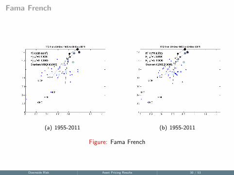
Fama French
(a) 1955-2011 (b) 1955-2011
Figure: Fama French
Downside Risk Asset Pricing Results 30 / 53

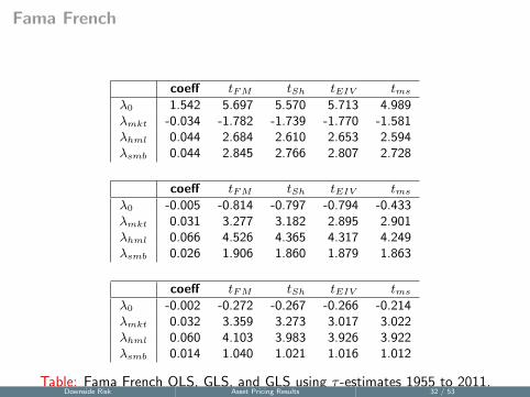
Fama French
coeff tFM tSh tEIV tms
γ0 1.542 5.697 5.570 5.713 4.989γmkt -0.644 -1.998 -1.966 -1.995 -1.799γhml 0.383 3.451 3.447 3.461 3.456γsmb 0.177 1.492 1.490 1.498 1.504
coeff tFM tSh tEIV tms
γ0 -0.005 -0.814 -0.797 -0.794 -0.433γmkt 0.473 2.763 2.763 2.763 2.780γhml 0.359 3.323 3.323 3.318 3.287γsmb 0.236 2.035 2.035 2.037 2.029
coeff tFM tSh tEIV tms
γ0 -0.002 -0.258 -0.260 -0.251 -0.197γmkt 0.463 28.507 2.695 7.398 7.303γhml 0.329 3.605 2.802 3.556 3.187γsmb 0.144 1.477 1.158 1.463 1.393
Table: Fama French OLS, GLS, and GLS using τ -estimates 1955 to 2011.Downside Risk Asset Pricing Results 31 / 53
Fama French
coeff tFM tSh tEIV tms
λ0 1.542 5.697 5.570 5.713 4.989λmkt -0.034 -1.782 -1.739 -1.770 -1.581λhml 0.044 2.684 2.610 2.653 2.594λsmb 0.044 2.845 2.766 2.807 2.728
coeff tFM tSh tEIV tms
λ0 -0.005 -0.814 -0.797 -0.794 -0.433λmkt 0.031 3.277 3.182 2.895 2.901λhml 0.066 4.526 4.365 4.317 4.249λsmb 0.026 1.906 1.860 1.879 1.863
coeff tFM tSh tEIV tms
λ0 -0.002 -0.272 -0.267 -0.266 -0.214λmkt 0.032 3.359 3.273 3.017 3.022λhml 0.060 4.103 3.983 3.926 3.922λsmb 0.014 1.040 1.021 1.016 1.012
Table: Fama French OLS, GLS, and GLS using τ -estimates 1955 to 2011.Downside Risk Asset Pricing Results 32 / 53

Fama French DSR
(a) 1955-2001 (b) 1955-2011
Figure: Fama French with DSR
Downside Risk Asset Pricing Results 33 / 53
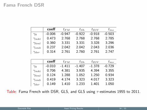
Fama French DSR
coeff tFM tSh tEIV tms
γ0 -0.006 -0.947 -0.922 -0.918 -0.503γmkt 0.473 2.768 2.768 2.768 2.785γhml 0.360 3.331 3.331 3.328 3.296γsmb 0.237 2.042 2.042 2.043 2.036γdsr 0.314 2.761 2.760 2.761 2.747
coeff tFM tSh tEIV tms
γ0 -0.010 -1.411 -1.407 -1.378 -0.729γmkt 0.706 4.381 3.935 4.394 3.355γhml 0.124 1.288 1.052 1.250 0.934γsmb 0.419 4.174 3.323 4.017 3.323γdsr 0.149 1.410 1.233 1.401 1.050
Table: Fama French with DSR, GLS, and GLS using τ -estimates 1955 to 2011.
Downside Risk Asset Pricing Results 34 / 53
Fama French DSR
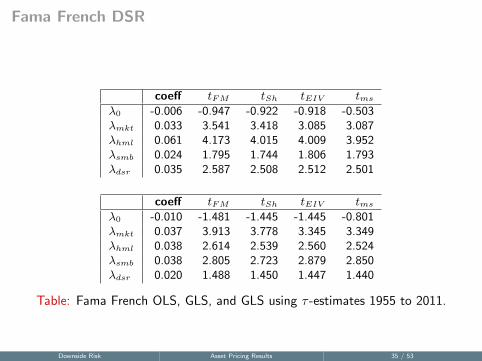
coeff tFM tSh tEIV tms
λ0 -0.006 -0.947 -0.922 -0.918 -0.503λmkt 0.033 3.541 3.418 3.085 3.087λhml 0.061 4.173 4.015 4.009 3.952λsmb 0.024 1.795 1.744 1.806 1.793λdsr 0.035 2.587 2.508 2.512 2.501
coeff tFM tSh tEIV tms
λ0 -0.010 -1.481 -1.445 -1.445 -0.801λmkt 0.037 3.913 3.778 3.345 3.349λhml 0.038 2.614 2.539 2.560 2.524λsmb 0.038 2.805 2.723 2.879 2.850λdsr 0.020 1.488 1.450 1.447 1.440
Table: Fama French OLS, GLS, and GLS using τ -estimates 1955 to 2011.
Downside Risk Asset Pricing Results 35 / 53
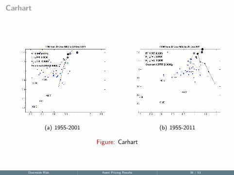
Carhart
(a) 1955-2001 (b) 1955-2011
Figure: Carhart
Downside Risk Asset Pricing Results 36 / 53
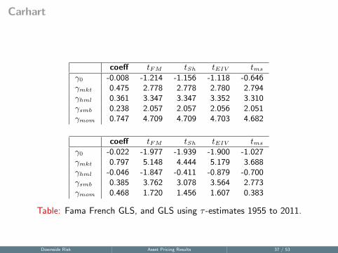
Carhart
coeff tFM tSh tEIV tms
γ0 -0.008 -1.214 -1.156 -1.118 -0.646γmkt 0.475 2.778 2.778 2.780 2.794γhml 0.361 3.347 3.347 3.352 3.310γsmb 0.238 2.057 2.057 2.056 2.051γmom 0.747 4.709 4.709 4.703 4.682
coeff tFM tSh tEIV tms
γ0 -0.022 -1.977 -1.939 -1.900 -1.027γmkt 0.797 5.148 4.444 5.179 3.688γhml -0.046 -1.847 -0.411 -0.879 -0.700γsmb 0.385 3.762 3.078 3.564 2.773γmom 0.468 1.720 1.456 1.607 0.383
Table: Fama French GLS, and GLS using τ -estimates 1955 to 2011.
Downside Risk Asset Pricing Results 37 / 53

Carhart
coeff tFM tSh tEIV tms
λ0 -0.008 -1.214 -1.156 -1.118 -0.646λmkt 0.041 4.331 4.073 3.404 3.414λhml 0.087 5.797 5.400 4.911 4.857λsmb 0.027 2.009 1.908 1.926 1.917λmom 0.060 6.211 5.767 4.262 4.216
coeff tFM tSh tEIV tms
λ0 -0.022 -3.421 -3.318 -3.272 -1.788λmkt 0.044 4.645 4.438 3.751 3.767λhml 0.031 2.080 2.011 1.910 1.888λsmb 0.030 2.236 2.160 2.211 2.187λmom 0.038 3.885 3.729 3.190 3.154
Table: Fama French GLS, and GLS using τ -estimates 1955 to 2011.
Downside Risk Asset Pricing Results 38 / 53

Carhart with DSR
(a) 1955-2001 (b) 1955-2011
Figure: Carhart with DSR
Downside Risk Asset Pricing Results 39 / 53
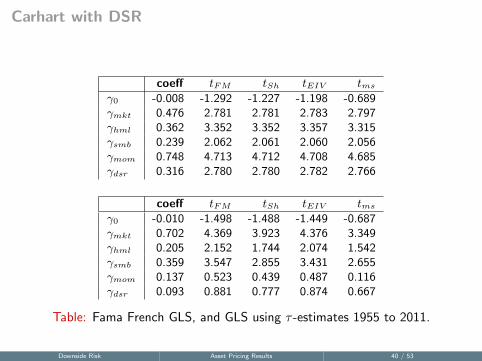
Carhart with DSR
coeff tFM tSh tEIV tms
γ0 -0.008 -1.292 -1.227 -1.198 -0.689γmkt 0.476 2.781 2.781 2.783 2.797γhml 0.362 3.352 3.352 3.357 3.315γsmb 0.239 2.062 2.061 2.060 2.056γmom 0.748 4.713 4.712 4.708 4.685γdsr 0.316 2.780 2.780 2.782 2.766
coeff tFM tSh tEIV tms
γ0 -0.010 -1.498 -1.488 -1.449 -0.687γmkt 0.702 4.369 3.923 4.376 3.349γhml 0.205 2.152 1.744 2.074 1.542γsmb 0.359 3.547 2.855 3.431 2.655γmom 0.137 0.523 0.439 0.487 0.116γdsr 0.093 0.881 0.777 0.874 0.667
Table: Fama French GLS, and GLS using τ -estimates 1955 to 2011.
Downside Risk Asset Pricing Results 40 / 53
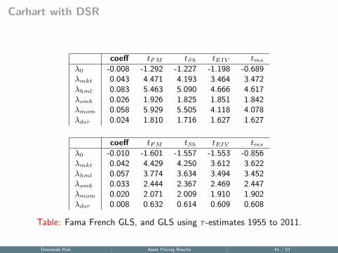
Carhart with DSR
coeff tFM tSh tEIV tms
λ0 -0.008 -1.292 -1.227 -1.198 -0.689λmkt 0.043 4.471 4.193 3.464 3.472λhml 0.083 5.463 5.090 4.666 4.617λsmb 0.026 1.926 1.825 1.851 1.842λmom 0.058 5.929 5.505 4.118 4.078λdsr 0.024 1.810 1.716 1.627 1.627
coeff tFM tSh tEIV tms
λ0 -0.010 -1.601 -1.557 -1.553 -0.856λmkt 0.042 4.429 4.250 3.612 3.622λhml 0.057 3.774 3.634 3.494 3.452λsmb 0.033 2.444 2.367 2.469 2.447λmom 0.020 2.071 2.009 1.910 1.902λdsr 0.008 0.632 0.614 0.609 0.608
Table: Fama French GLS, and GLS using τ -estimates 1955 to 2011.
Downside Risk Asset Pricing Results 41 / 53

Petkova
(a) 1955-2001 (b) 1955-2011
Figure: Petkova
Downside Risk Asset Pricing Results 42 / 53
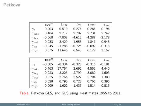
Petkova
coeff tFM tSh tEIV tms
γ0 0.003 0.519 0.276 0.266 0.196γmkt 0.464 2.712 2.707 2.731 2.742γdvy -0.060 -7.808 -4.612 -4.287 -2.178γcrd 0.033 3.429 1.955 1.846 0.945γslp -0.045 -1.288 -0.725 -0.692 -0.313γrfr 0.075 11.646 6.543 6.172 3.157
coeff tFM tSh tEIV tms
γ0 -0.005 -0.334 -0.328 -0.316 -0.181γmkt 0.463 27.754 2.692 4.553 4.440γdvy -0.023 -3.225 -2.799 -3.080 -1.603γcrd 0.025 2.766 2.527 2.794 1.383γslp 0.028 0.790 0.728 0.765 0.395γrfr -0.009 -1.602 -1.435 -1.514 -0.815
Table: Petkova GLS, and GLS using τ -estimates 1955 to 2011.
Downside Risk Asset Pricing Results 43 / 53
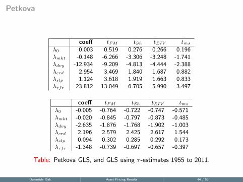
Petkova
coeff tFM tSh tEIV tms
λ0 0.003 0.519 0.276 0.266 0.196λmkt -0.148 -6.266 -3.306 -3.248 -1.741λdvy -12.934 -9.209 -4.813 -4.444 -2.388λcrd 2.954 3.469 1.840 1.687 0.882λslp 1.124 3.618 1.919 1.663 0.833λrfr 23.812 13.049 6.705 5.990 3.497
coeff tFM tSh tEIV tms
λ0 -0.005 -0.764 -0.722 -0.747 -0.571λmkt -0.020 -0.845 -0.797 -0.873 -0.485λdvy -2.635 -1.876 -1.768 -1.902 -1.003λcrd 2.196 2.579 2.425 2.617 1.544λslp 0.094 0.302 0.285 0.292 0.173λrfr -1.348 -0.739 -0.697 -0.657 -0.397
Table: Petkova GLS, and GLS using τ -estimates 1955 to 2011.
Downside Risk Asset Pricing Results 44 / 53
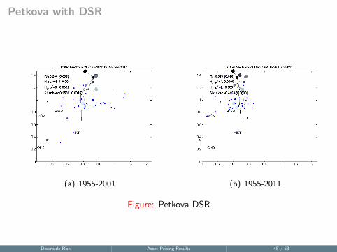
Petkova with DSR
(a) 1955-2001 (b) 1955-2011
Figure: Petkova DSR
Downside Risk Asset Pricing Results 45 / 53

Petkova with DSR
coeff tFM tSh tEIV tms
γ0 0.003 0.459 0.246 0.238 0.175γmkt 0.464 2.714 2.709 2.733 2.745γdvy -0.059 -7.593 -4.495 -4.106 -2.062γdsr 0.305 2.680 2.668 2.665 2.647γcrd 0.031 3.127 1.784 1.728 0.830γslp -0.041 -1.163 -0.657 -0.618 -0.278γrfr 0.074 11.570 6.533 6.188 3.124
coeff tFM tSh tEIV tms
γ0 0.002 0.147 0.131 0.122 0.042γmkt 0.415 2.685 2.165 2.464 1.875γdvy -0.003 -0.422 -0.347 -0.349 -0.113γdsr -0.085 -0.850 -0.673 -0.770 -0.582γcrd 0.032 3.517 2.905 2.971 0.924γslp 0.019 0.557 0.465 0.467 0.127γrfr 0.029 5.197 4.281 4.267 1.163
Table: Petkova DSR, GLS, and GLS using τ -estimates 1955 to 2011.Downside Risk Asset Pricing Results 46 / 53

Petkova with DSR
coeff tFM tSh tEIV tms
λ0 0.003 0.459 0.246 0.238 0.175λmkt -0.144 -5.979 -3.174 -3.041 -1.615λdvy -12.741 -8.917 -4.692 -4.251 -2.249λdsr 0.010 0.736 0.393 0.384 0.313λcrd 2.748 3.066 1.637 1.539 0.754λslp 1.160 3.688 1.967 1.682 0.838λrfr 23.749 13.000 6.717 6.035 3.483
coeff tFM tSh tEIV tms
λ0 0.002 0.338 0.286 0.276 0.149λmkt 0.028 1.156 0.977 0.883 0.314λdvy -0.441 -0.308 -0.261 -0.234 -0.079λdsr -0.019 -1.345 -1.136 -1.099 -0.681λcrd 2.973 3.317 2.790 2.920 0.933λslp 0.699 2.222 1.875 1.730 0.558λrfr 9.281 5.080 4.240 4.235 1.439
Table: Petkova GLS, and GLS using τ -estimates 1955 to 2011.Downside Risk Asset Pricing Results 47 / 53
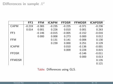
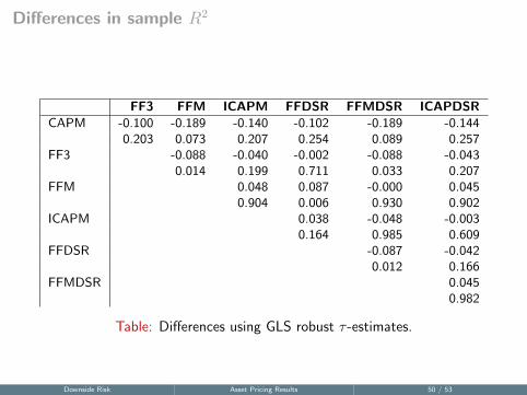
Differences in sample R2
FF3 FFM ICAPM FFDSR FFMDSR ICAPDSRCAPM -0.219 -0.365 -0.235 -0.225 -0.371 -0.236
0.014 0.001 0.226 0.010 0.001 0.263FF3 -0.146 -0.015 -0.005 -0.152 -0.016
0.000 0.008 0.273 0.000 0.012FFM 0.131 0.141 -0.006 0.130
0.239 0.000 0.251 0.129ICAPM 0.010 -0.136 -0.001
0.009 0.228 0.815FFDSR -0.146 -0.011
0.000 0.013FFMDSR 0.135
0.121
Table: Differences using GLS.
Downside Risk Asset Pricing Results 48 / 53
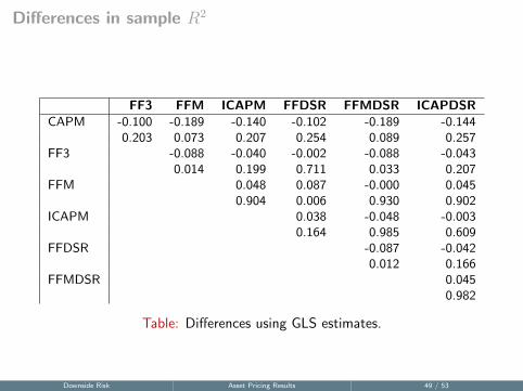
Differences in sample R2
FF3 FFM ICAPM FFDSR FFMDSR ICAPDSRCAPM -0.100 -0.189 -0.140 -0.102 -0.189 -0.144
0.203 0.073 0.207 0.254 0.089 0.257FF3 -0.088 -0.040 -0.002 -0.088 -0.043
0.014 0.199 0.711 0.033 0.207FFM 0.048 0.087 -0.000 0.045
0.904 0.006 0.930 0.902ICAPM 0.038 -0.048 -0.003
0.164 0.985 0.609FFDSR -0.087 -0.042
0.012 0.166FFMDSR 0.045
0.982
Table: Differences using GLS estimates.
Downside Risk Asset Pricing Results 49 / 53
Differences in sample R2
FF3 FFM ICAPM FFDSR FFMDSR ICAPDSRCAPM -0.100 -0.189 -0.140 -0.102 -0.189 -0.144
0.203 0.073 0.207 0.254 0.089 0.257FF3 -0.088 -0.040 -0.002 -0.088 -0.043
0.014 0.199 0.711 0.033 0.207FFM 0.048 0.087 -0.000 0.045
0.904 0.006 0.930 0.902ICAPM 0.038 -0.048 -0.003
0.164 0.985 0.609FFDSR -0.087 -0.042
0.012 0.166FFMDSR 0.045
0.982
Table: Differences using GLS robust τ -estimates.
Downside Risk Asset Pricing Results 50 / 53
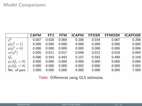
Model Comparisons
CAPM FF3 FFM ICAPM FFDSR FFMDSR ICAPDSRρ̂2 0.007 0.028 0.064 0.206 0.034 0.067 0.206p(ρ2 = 1) 0.000 0.000 0.000 0.000 0.000 0.000 0.000p(ρ2 = 0) 0.006 0.000 0.000 0.005 0.000 0.000 0.006se(ρ̂2) 0.005 0.011 0.017 0.094 0.012 0.018 0.093
Q̂c 0.596 0.593 0.493 0.157 0.593 0.490 0.159p1(Qc = 0) 0.000 0.000 0.000 0.000 0.000 0.000 0.000p2(Qc = 0) 0.000 0.000 0.000 0.002 0.000 0.000 0.002No. of pars 2.000 4.000 5.000 6.000 5.000 6.000 7.000
Table: Differences using GLS estimates.
Downside Risk Asset Pricing Results 51 / 53
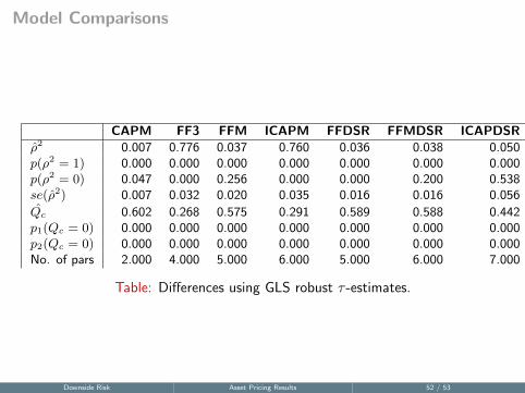
Model Comparisons
CAPM FF3 FFM ICAPM FFDSR FFMDSR ICAPDSRρ̂2 0.007 0.776 0.037 0.760 0.036 0.038 0.050p(ρ2 = 1) 0.000 0.000 0.000 0.000 0.000 0.000 0.000p(ρ2 = 0) 0.047 0.000 0.256 0.000 0.000 0.200 0.538se(ρ̂2) 0.007 0.032 0.020 0.035 0.016 0.016 0.056
Q̂c 0.602 0.268 0.575 0.291 0.589 0.588 0.442p1(Qc = 0) 0.000 0.000 0.000 0.000 0.000 0.000 0.000p2(Qc = 0) 0.000 0.000 0.000 0.000 0.000 0.000 0.000No. of pars 2.000 4.000 5.000 6.000 5.000 6.000 7.000
Table: Differences using GLS robust τ -estimates.
Downside Risk Asset Pricing Results 52 / 53

Conclusions and musings
Downside Risk Conclusion 53 / 53