Embed Size (px)
Citation preview
ii
Mahadevan Ilankatharan
December 2008
Civil and Environmental Engineering
Centrifuge Modeling for Soil-Pile-Bridge Systems with Numerical Simulations
Accounting for Soil-Container-Shaker Interaction
Abstract
Centrifuge testing of soil-pile-bridge systems was conducted using the NEES
(Network of Earthquake Engineering Simulation) geotechnical centrifuge at UC Davis.
This testing was a part of a multi-university and multi-disciplinary collaborative research
utilizing NEES with goal of investigating the effects of Soil-Foundation-Structure-
Interaction (SFSI) while demonstrating NEES research collaboration. The centrifuge
experiments complement the 1-g shake table and field experiments conducted at other
universities. The data from the centrifuge experiments was compared and combined with
the data from other universities to provide integrated analytical models for SFSI problems
of soil-pile-bridge systems. This dissertation presents results of these experiments,
including collaborations, comparisons with other experiments and numerical simulations,
and end-to-end usage of data. Although many aspects of the collaboration exercise were
successful, one conclusion of this part of the work was that significant discrepancies
between simulations and experiments may be caused by soil-container-shaker interaction
in the experiments.
Some aspects of the interaction between the shaker and the specimen were
accounted for by implementing in the OpenSees finite element simulations a novel
method for simulating the excitation of the shaking table as a dynamic force in the
iii
actuator (flexible-actuator-prescribed force approach) instead of the conventional
approach of specifying the excitation as a prescribed- displacement of the shaking table.
Other aspects of the interaction were accounted for by including a more accurate model
of the model container, bearing, and reaction mass of the system. Initial attempts to
include the servo-hydraulic control system in the simulations were attempted.
Based on a systematic series of simulations of the site response of the centrifuge
model that included different approximations of the centrifuge-shaker system, it was
concluded that the sensitivity of simulation results to uncertainties in modeling
parameters depends on how the aspects of soil-container-shaker interaction are accounted
for. This raises a fundamental and very general question: How can we assess the
significance of a discrepancy between a simulation and an experimental result? Although
this dissertation does not provide a general answer to this fundamental question, it does
show that for centrifuge-shaking table experiments, the significance of errors in the
simulations cannot be rigorously assessed without accounting for test specimen-actuation
system interaction. The archives of centrifuge test data and metadata and OpenSees
numerical models of soil-container-shaker system are available for others to use at the
NEEScentral website (http://central.nees.org).

iv
Dedication
To my mom

v
Acknowledgements
This dissertation research was supported by NSF awards CMS-0324343 and
CMS-0402490 through the George E. Brown, Jr. Network for Earthquake Engineering
Simulations (NEES). Without the support of NEES and the NSF, this research would not
have been possible. Any opinions, findings and conclusions or recommendations
expressed in this dissertation are those of the author and do not necessarily reflect those
of the NSF. The centrifuge shaker was designed and constructed with support from the
NSF, Obayashi Corp., Caltrans and the University of California. Recent upgrades have
been funded by NSF award CMS-0086566 through NEES.
Through my education, a great number of people have helped me to get where I
am today. Without all of your support and guidance, none of this would have been
possible.
First and foremost, I would like to express my gratitude to my supervisor, Prof.
Bruce Kutter. Prof. Kutter has guided me in several aspects of my development as a
graduate student, not only by giving me the opportunity to pursue exciting and relevant
research but also by teaching me how to present my work in a precise and elegant
manner. His dedication and love for research and academic excellence have rubbed off on
me. I am really glad and proud that I have had an opportunity to work closely with such a
wonderful person.
I would like to acknowledge my dissertation committee members Professor Ross
Boulanger and Professor Boris Jeremić for their valuable comments and suggestions.
Their inputs have helped to improve the research and the quality of this dissertation.
I would like to thank Center for Geotechnical Modeling (CGM) facility manger
Dr. Dan Wilson for his guidance and support on this research, and CGM staff Lars
Pedersen, Chard Justice, Tom Kohnke, Tom Coker, and Cypress Winters, for their help in
different ways for my research work.
I would like to thank my research collaborators from the University of Washington,
Dr. Hysung-Suk Shin and Professors Pedro Arduino and Steve Kramer and the collaborators

vi
from other universities for sharing their valuable simulation and experimental data and ideas
in the course of this research.
I have had so many wonderful teachers throughout my education who directly or
indirectly contributed to my doctoral degree. I am very grateful to all my teachers at St.
Henry’s college, Ilavalai, Sri Lanka; the University of Peradeniya, Sri Lanka; and the
University of California, Davis.
I am very obliged to the help and support provided by my uncle Santhanasamy and
family, and many relatives and friends during my college and high school years in Sri Lanka.
I would like to thank my friend Sathishbalamurugan for his help and motivation and
helping me to “stay positive” during my university years in Sri Lanka and Davis.
I wish to express my sincere gratitude to my parents for always giving top priority
to my education. My aunt, Lilly, always helped and encouraged me to achieve my
educational goals, I am very thankful to her. Without my mother’s patience and
determination and my Aunt’s guidance and support, I would not have been in a position
to write this dissertation.
Last, but not least, I would like to thank my wife, Jocy, for patiently helping me in
many ways to complete my research and dissertation.
vii
Table of Contents
Page
Abstract ii
Acknowledgements v
List of Figures xv
List of Tables xxx
Chapter 1: Introduction 1
1.1 Background 1
1.1.1 Centrifuge testing of soil-foundation-bridge systems 1
1.1.2 Soil – container – centrifuge shaker interaction 4
1.2 Scope of the dissertation 5
1.3 Organization of dissertation 7
Chapter 2: Collaborative research: Centrifuge testing of soil-pile-bridge
systems 14
2.1 NEES collaborative research project to study SFSI 15
2.1.1 Field tests 16
2.1.2 Structural component tests 16
2.1.3 1-g shake table experiment 16
2.1.4 Centrifuge experiments 17
viii
2.2 Centrifuge test program 17
2.2.1 Concept of the geotechnical centrifuge modeling 17
2.2.2 Model configurations 18
2.2.2.1 Centrifuge test series MIL01 18
2.2.2.2 Centrifuge test series MIL02 19
2.2.2.3 Centrifuge test series MIL03 19
2.2.3 Design of structural models 20
2.2.4 Model preparation and instrumentation 21
2.2.5 Ground motion protocols 23
2.3 Representative results from centrifuge experiments 23
2.3.1 Soil site response 23
2.3.2 Horizontal accelerations 24
2.3.3 Vertical accelerations 24
2.3.4 Bending moment, shear force and sub-grade reaction 25
2.3.5 Superstructure accelerations of MIL02 bridge bents 25
2.4 Comparisons with UT Austin field tests 26
2.5 Simulations of centrifuge models 27
2.5.1 Outline of simulation models 27
2.5.2 Predicted site response 28
2.5.3 Predicted response of individual bents and single pile 29
2.5.4 Predicted response of two-span bridge model 30
2.5.5 Sensitivity analyses 31
2.5.6 Simulations of MIL02 and MIL03 test series 32
ix
2.6 Simulation of the prototype bridge structure 32
2.7 Centrifuge test data archives 33
2.8 Summary 34
2.8.1 Research collaboration 34
2.8.2 Centrifuge experiments 35
2.8.3 Simulations of centrifuge experiments 36
2.8.4 Effect of modeling boundary conditions on the sensitivity of
predicted site response 37
Chapter 3: Comparison of centrifuge and 1g shake table models of a
pile supported bridge structure 79
3.1 Introduction 81
3.2 Centrifuge and Shake table bridge models 83
3.2.1 General test setup 83
3.2.2 Scale factors for 1/52 scale centrifuge model and ¼ scale 1-g
shake table model 84
3.2.3 Pile properties 84
3.2.4 Design for above ground clear heights 85
3.2.5 Deck properties and spacing between bents 86
3.2.6 Selection of input motion and testing sequence 87
3.3 Comparison of centrifuge and 1g shake table experimental results 88
x
3.3.1 During a medium level shaking event (peak base acc = 0.25 g in
centrifuge test) 88
3.3.2 During a large level shaking event (peak base acc = 0.78 g in
centrifuge test) 89
3.4 Comparison of the system (three-bent) response to the individual bent
response in the centrifuge experiment 90
3.5 Conclusions 92
3.6 References 94
Chapter 4: Modeling input motion boundary conditions for simulations of
geotechnical shaking table tests 118
4.1 Introduction 120
4.2 Modeling of a soil column mounted on a centrifuge shaking table 122
4.2.1 Representing input motion boundary conditions 123
4.2.1.1 Prescribed-force simulation 123
4.2.1.2 Prescribed-displacement simulation 124
4.2.2 Soil model 125
4.2.3 Shaker and reaction mass 125
4.2.4 Selection of damping parameters and input variables 127
4.3 Simulation results 128
4.3.1 Linear elastic soil material model simulations 128
4.3.2 Elasto- plastic PDMY soil material model simulations 132
xi
4.4 Parametric studies 134
4.4.1 Effect of ξact 134
4.4.2 Effect of ξsoil 135
4.4.3 Effect of kact & MRM 136
4.5 Ground motion analogy: Rigid and Compliant base 137
4.6 Discussion 139
4.6.1 Importance of proper treatment of boundary conditions on the
sensitivity analysis 139
4.6.2 Need for realistic numerical models of servo-hydraulic actuation
system 140
4.7 Conclusions 141
4.8 Acknowledgements 143
4.9 References 143
Chapter 5: Numerical modeling of a soil-model container-centrifuge
shaking table system 160
5.1 Introduction 162
5.2 Modeling system components 163
5.2.1 Soil Model 164
5.2.2 Model container 165
5.2.3 Shaker and Reaction mass 166
5.3 Boundary conditions in simulation models 168
xii
5.3.1 1-D shear beam simulations of soil 168
5.3.2 2-D simulations of soil and container 168
5.3.3 2-D simulations of soil, container, and shaker 168
5.4 Simulation results 169
5.4.1 Soil horizontal accelerations from 1-D shear beam simulations of
soil and 2-D simulations of soil and container 169
5.4.2 Soil Vertical accelerations from 2-D simulations of soil and
container 170
5.4.3 Results from the 2-D simulations of soil, container, and shaker 171
5.5 Sensitivity analysis 173
5.6 Archives of numerical models of a soil-container-shaker system 175
5.7 Summary 176
5.8 References 178
Chapter 6: Towards developing a numerical model of a servo-hydraulic
centrifuge actuation system to predict shake table response 203
6.1 Factors affecting the reproduction of a dynamic signal in a
servo-hydraulic actuation system 204
6.2 Analytical models for various components of servo-hydraulic actuation
system 205
6.3 Outline of servo-hydraulic actuation system of the UC Davis centrifuge
facility 208
xiii
6.4 Current base motion tuning procedures 209
6.5 Modifications to the shaker model presented in chapter 5 212
6.5.1 To account for the effects of feed-back controller 212
6.5.2 To account for the oil pressure limit and the limit on oil flow
velocity 213
6.5.3 To account for servo-valve nonlinearity 214
6.6 Simulated base response 214
6.7 Discussion on the simulation results and the need for additional work 217
Chapter 7: Summary and Conclusions, and Future work 233
7.1 Summary and Conclusions 233
7.1.1 Collaborative research: Centrifuge testing of soil-pile-bridge
systems 233
7.1.1.1 Research collaborations 234
7.1.1.2 Centrifuge experiments 235
7.1.1.3 Centrifuge test data archives 238
7.1.1.4 Numerical simulations of the centrifuge experiments 238
7.1.2 Modeling input motion boundary conditions for simulations of
geotechnical shaking table experiments 240
7.1.3 Numerical simulations of the soil model accounting for
soil-container-shaker interaction 242

xiv
7.1.4 Numerical model of a servo-hydraulic centrifuge actuation system
to predict shaking table response 244
7.2 Areas for future research 246
References 249
Appendix A: Centrifuge test and simulation data archives 258
xv
List of Figures
Page
Chapter 1
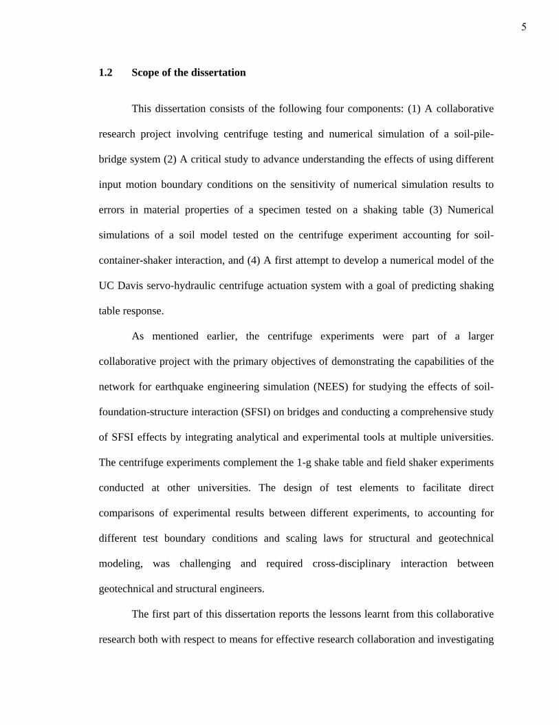
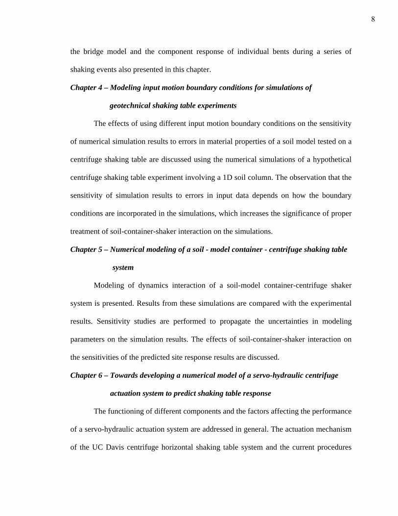
1.1: Collapse of San Francisco/Oakland Bay bridge section, 1989 Loma Prieta
earthquake 10
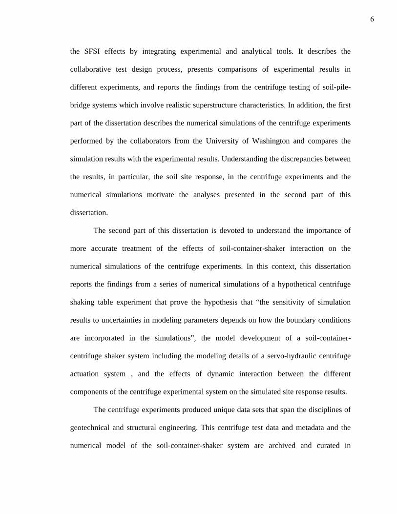
1.2: Unseating of bridge span, Nishinomiya ki bridge, 1995 Kobe earthquake 10
1.3: Schematic of a bridge supported on pile foundations shows wide variations in
structural types/configurations and soil conditions (after Martin et al. 2002) 11
1.4: Schematic of Soil-Foundation-Structure-Interaction (SFSI) phenomena for
a pile supported structure (modified from Gazetas et al. 1998) 11
1.5: Overview of the NEES collaborative project to study
soil-foundation-structure-interaction 12
1.6: 3D rendering of a soil model-model container-centrifuge shaking table
system 13
1.7: Representation of soil-container-shaker interaction (after Kutter, 1994) 13
Chapter 2
2.1: Overview of the earthquake engineering components of the NEES
collaborative project to study soil-foundation-structure-interaction 42
2.2: Example of prototype location in a multi-span bridge 42
2.3: Seismic excitation of the field test specimen using T-Rex (after Black 2005) 43
xvi
2.4: Seismic excitation of the field test specimen using Thumper
(after Black 2005) 43
2.5: (a) 3-D rendering of test set-up and (b) photograph of a test specimen of the
structural component tests at the Purdue University (after Makido 2007) 44
2.6: (a) 3-D rendering of test set-up and (b) photograph of a test specimen of the
1-g shaking table experiment (after Johnson 2006) 45
2.7: Photograph of the 1/52 scale models of the test specimens used in the first
series of centrifuge experiments 46
2.8: 3-D rendering of model layout of the centrifuge test series MIL01 46
2.9: Details of structural models in MIL01 test series 47
2.10: (a) Schematic and (b) Rendering of model layout of MIL02 test series 48
2.11: (a) Schematic and (b) Rendering of model layout of MIL03 test series 49
2.12: Configurations and embedment lengths of structural models used in MIL03
test series 50
2.13: Shear Wave Velocity Profile of Capitol Aggregate Test Site, Austin and
Nevada Sand (Dr = 80%) 51
2.14: Instrumentation layout in one of the centrifuge test series 52
2.15: Photograph from one of the centrifuge test series showing the
instrumentation using the high-speed video cameras and high-speed
wireless data acquisition system 53
2.16: Comparison of data recorded by traditional wired data acquisition system
and the new wireless data acquisition system at UC Davis
(after Wilson et al. 2007) 54
xvii
2.17: Time histories and response spectra of Northridge and frequency sweep
motions used in the centrifuge test series 55
2.18: Measured soil accelerations from a vertical array of horizontal accelerometers
in test MIL03 (Northridge input motion, peak base acceleration = 0.26 g) 56
2.19: Measured horizontal motions at different locations of model in MIL01 test
series (Northridge input motion, peak base acceleration = 0.23 g) 57
2.20: Measured vertical motions at the container base & 2.6m from ground surface
in MIL03 test series (Northridge input motion, peak base acceleration
= 0.26 g) 58
2.21: Bending moment, shear force, and sub-grade reaction of bridge bents
@ time of maximum bent-cap displacement (Northridge input motion,
peak base acceleration = 0.57 g) 59
2.22: Normalized depth to maximum bending moment for different
above-ground clear height bridge bents in MIL01 test series 60
2.23: Response of bridge bents oriented different directions to base shaking in
MIL02 test series (frequency sweep input motion 7-333Hz) 61
2.24: Response of bridge bents in the centrifuge and field tests to the base
excitation in the transverse direction of the bent (frequency sweep input) 62
2.25: Seismic excitation directions for (a) centrifuge test specimen, and (b) field
test specimen 63
2.26: Modeling of soil-pile-structure interaction in a single pile using p-y, t-z,
and Q-z springs in OpenSees (after Shin 2007) 64
xviii
2.27: Numerical modeling of the two-span bridge model in MIL01 test series
using OpenSees (after Shin 2007) 64
2.28: Response spectra of measured (CFG) and simulated (Open) horizontal
free-field soil accelerations in MIL02 test series (after Shin et al. 2006) 65
2.29: Time histories of measured and simulated horizontal free-field soil
accelerations in MIL03 test series; Northridge input motion, peak base
acceleration = 0.26 g (after Shin 2007) 66
2.30: Ratios of Fourier amplitudes between the horizontal soil motion @ 2.6m
and the horizontal base motion in MIL03 test series and OpenSees 1-D
shear beam simulations; frequency sweep input motion, peak base
acceleration = 0.25 g (after Shin 2007) 67
2.31: Time histories and Fourier amplitude of measured and calculated horizontal
motions at the bent-cap of a two-pile individual bent (Bent 5) in MIL01 test
series; Northridge input motion, peak base acc = 0.25 g (after Shin 2007) 68
2.32: Measured and calculated maximum pile bending moment of Bent 5
in MIL01 test series; Northridge input motion, peak base acceleration =
0.25 g (after Shin 2007) 68
2.33: Measured and calculated peak accelerations of superstructure and at 2.5m
below ground surface in MIL01 test series during different intensity base
motions (after Shin 2007) 69
xix
2.34: Time histories of measured and calculated horizontal motions at the
bent-caps of the two-span bridge model in MIL01 test series; Northridge
input motion, peak base acc=0.25g (after Shin et al. 2006) 70
2.35: Measured and predicted response of the two-span bridge model in MIL01
test series; Northridge input motion, peak base acceleration = 0.25 g (after
Shin et al. 2006) 71
2.36: Back calculated ultimate soil resistance from pile bending moment data in
the centrifuge test and the ultimate soil resistance obtained from p-y spring
forces in the OpenSees simulations, @ time of maximum bent-cap displace
ment (after Shin et al. 2006) 72
2.37: Regions of p-y spring parameters considered in the sensitivity analyses (after
Shin 2007) 73
2.38: Sensitivity analysis: Effect of soil motion on bent response, Northridge
motion peak base acceleration = 0.25g (after Shin 2007) 74
2.39: Sensitivity analysis: Effect of ultimate soil resistance (pult) on bent response,
Northridge motion peak base acc = 0.25 g (after Shin 2007) 75
2.40: 3-D finite element model of the prototype soil-pile-bridge system (after Jie
2007) 76
2.41: End-to-end data usage scenario (after Van Den Einde et al. 2007) 77
2.42: End-to-end usage of centrifuge test data (screen shot from UCDavis-N3DV
data viewer, after Kutter 2007) 78
xx
Chapter 3
3.1: Hypothetical prototype multi-span bridge 98
3.2: Layout of the bridge model in the centrifuge test series 99
3.3: Photograph of bridge model set-up on centrifuge model container 100
3.4: Layout of the bridge model in the 1g shake table experiment (Wood et al.
2004) 101
3.5: Photograph of bridge model set-up on shake tables at the University of
Nevada, Reno (after Johnson et al. 2006) 102
3.6: Typical pile cross section in the centrifuge experiment 103
3.7: Calculation of clear heights of piles based on equivalent cantilever model 104
3.8: Load, shear and bending moment diagrams for pile in the ground and column
on the shake table at ultimate state 105
3.9: Time histories and response spectra of base motions before and after
tuning and amplitude of tuning transfer function for base motion (peak
base acc = 0.23 g) 106
3.10: Time histories & acceleration response spectra of target & achieved free
field motion @ 50 mm below ground surface (before and after tuning, peak
base acc = 0.23 g) 107
3.11: Deck motions during a medium level shaking event (peak base acc= 0.25 g
in centrifuge test) 108
xxi
3.12: Response spectra of (5% damping) of free field motions @ 2.5 m depth in
the centrifuge test & shake table base motions, and deck motions during
medium level shaking event (peak base acc = 0.25 g in centrifuge test) 109
3.13: Deck displacements during a medium level shaking event (peak base acc =
0.25g) 110
3.14: Ratio of spectral accelerations (5% damping): deck motions to free field soil
motions @ 2.5 m in the centrifuge test and deck motions to table motions in
the 1g shake table test (peak base acc = 0.25 g in centrifuge test) 111
3.15: Column strains (bending) at 1.3m below deck level during a medium level
shaking event (peak base acc = 0.25 g) 112
3.16: Response spectra of (5% damping) of free field motions @ 2.5 m depth in
centrifuge test & shake table motions, and deck motions in both experiments
during a large amplitude shaking event (peak base acc = 0.78 g in centrifuge
test) 113
3.17: Ratio of spectral accelerations (5% damping): deck motions to free field soil
motions @ 2.5 m in the centrifuge experiment and deck motions to shake table
motions in the 1g shake table experiment (peak base acc = 0.78 g in centrifuge
test) 114
3.18: Response spectra of the base input motions for two centrifuge shaking events,
one applied before attaching the bridge deck, and one after connecting the
bridge deck to the bridge bents 115
3.19: Response spectra of the bridge bent accelerations before and after attaching
the bridge deck 116
xxii
3.20: Comparison of bending moment distributions in the columns/piles before
(single bents) and after (bridge bents) attaching the bridge deck 117
Chapter 4
4.1: 3D rendering of a soil model-container-centrifuge shaking table system 147
4.2: Reflection and refraction of seismic waves at the container base 147
4.3: Different input motion boundary conditions in the simulations 148
4.4: Configuration of the actuator elements 148
4.5: Time histories of (a) command acceleration, and (b) command displacement
of the input motion 149
4.6: Calculated frequency dependent soil damping ratio (ξsoil) by combining
stiffness proportional and mass proportional damping: an example case for
ξsoil = 2.5% at the first and the third modal frequencies (50 Hz and 250 Hz) 149
4.7: Time histories and response spectra (5% damping) of surface and base motions
in the prescribed-force and prescribed-displacement simulations employing a
linear elastic soil material 150
4.8: Time histories and response spectra (5% damping) of surface and base motions
in the prescribed-force and prescribed-displacement simulations employing a
linear elastic soil material (Gassumed/Gactual = 0.64) 150
4.9: Ratios of Fourier amplitudes between the surface motion and the base motion,
and base motion and command acceleration, in the prescribed-force and prescribed-
displacement simulations employing linear elastic soil material 151
xxiii
4.10: Sensitivity of peak & peak spectral accelerations of surface and base motions
to error in Gassumed of elastic soil material in the prescribed-force and prescribed-
displacement simulations 152
4.11: Time histories of motions at ground surface and at base of the soil column in
the prescribed-force and prescribed-displacement simulations employing the
elasto-plastic PDMY soil material 153
4.12: Time histories of motions at ground surface and at base of the soil column in
the prescribed-force and prescribed-displacement simulations employing the
elasto-plastic PDMY soil material (amplitude of the input motion 10 times
larger than that shown in Fig. 4.5) 153
4.13: Ratios of Fourier amplitudes between the surface motion and the base motion,
and the base motion and the command acceleration, in the prescribed-force and
prescribed-displacement simulations employing the elasto-plastic PDMY soil
material (simulations using the larger input motion) 154
4.14: Sensitivity of calculated peak acceleration of (a) surface motion, and (b) base
motion to error in Gr_assumed of the PDMY soil material in the prescribed-force &
prescribed-displacement simulations (simulations using the larger input
motion) 154
xxiv
4.15: Sensitivity of calculated peak acceleration of surface and base motions to
error in Gassumed of elastic soil material in the prescribed-force and prescribed-
displacement simulations, for different ξact values (ξsoil = 2.5%, ,1/
=HGA
kact
)5.0=RM
soil
MM
and
155
4.16: Sensitivity of calculated peak acceleration of surface and base motions to
error in Gassumed of elastic soil material in the prescribed-force and prescribed-
displacement simulations, for different ξsoil values (ξact = 20%, ,1/
=HGA
kact
)5.0=RM
soil
MM
and
156
4.17: ARS (5% damping) of calculated surface and base motions in the prescribed-force
and prescribed-displacement simulations, involving relatively stiff actuator and
heavy reaction mass ( ,20/
=HGA
kact 1.0=RM
soil
MM
and ), for different Gassumed values of
linear elastic soil material (ξact = 20%, and ξsoil = 2.5%) 157
4.18: Procedures for deconvolution of input motion for FLAC model described in
Mejia et al. 2006 158
4.19: (a) Time histories and (b) response spectrum of computed acceleration at top
of soil column for rigid base, and compliant base with 5% velocity mismatch
(Mejia et al. 2006) 159
xxv
Chapter 5
5.1: Photograph of the NEES geotechnical centrifuge at UC Davis 181
5.2: 3D rendering of a soil model-model container-centrifuge shaking table system181
5.3: Estimated damping ratios based on employed stiffness-proportional damping 182
5.4: Photographs of the FSB2 centrifuge model container 183
5.5: Dimensions and weights of different rings of the FSB2 container 184
5.6: Plan view of the horizontal shake table system at the UC Davis centrifuge
facility 185
5.7: 2D finite element mesh of the soil-model container-centrifuge shaker system 186
5.8: Configuration of actuator elements 186
5.9: Different boundary conditions in simulation models 187
5.10: Time histories of (a) measured acceleration at the base of the container
and (b) calculated displacement by double integration of acceleration of
the frequency sweep input (measured peak base acc = 1.3 g) 188
5.11: Measured and computed acceleration time histories and response spectra
(5% damping) from 1-D shear beam simulations of soil (frequency sweep
input, peak base acc = 1.3 g) 189
5.12: Measured and computed acceleration time histories and response spectra
(5% damping) from 1-D shear beam simulations of soil (Northridge input,
peak base acc = 1.3 g) 190
5.13: Measured and computed acceleration time histories and response spectra
(5% damping) from 2-D simulations of soil and container (frequency sweep
input, peak base acc = 1.3 g) 191
xxvi
5.14: Measured and computed acceleration time histories and response spectra
(5% damping) from 2-D simulations of soil and container (Northridge input,
peak base acc = 1.3 g) 192
5.15: Measured and computed vertical acceleration histories and response spectra
(5% damping) from 2-D simulations of soil and container (frequency sweep
input, peak base acc = 1.3 g) 193
5.16: Computed vertical acceleration histories and response spectra (5% damping)
in the 2-D simulations of soil and container, with & without shear rod 194
5.17: Measured and computed acceleration time histories and response spectra
(5% damping) from 2-D simulations of soil, container, and shaker (frequency
sweep input, peak base acc = 1.3 g) 195
5.18: Measured and computed base acceleration time histories and response spectra
(5% damping) from 2-D simulations of soil, container, and shaker (frequency
sweep input, peak base acc = 1.3 g) 196
5.19: Measured and computed base acceleration time histories and response spectra
(5% damping) from 2-D simulations of soil, container, and shaker (with
modified command displacement) 196
5.20: Measured and computed acceleration time histories and response spectra
(5% damping) from 2-D simulations of soil, container, and shaker (with
modified command displacement) 197
5.21: Ratio of Fourier amplitudes between the calculated and measured base
accelerations from 2-D simulations of soil, container, and shaker 198
xxvii
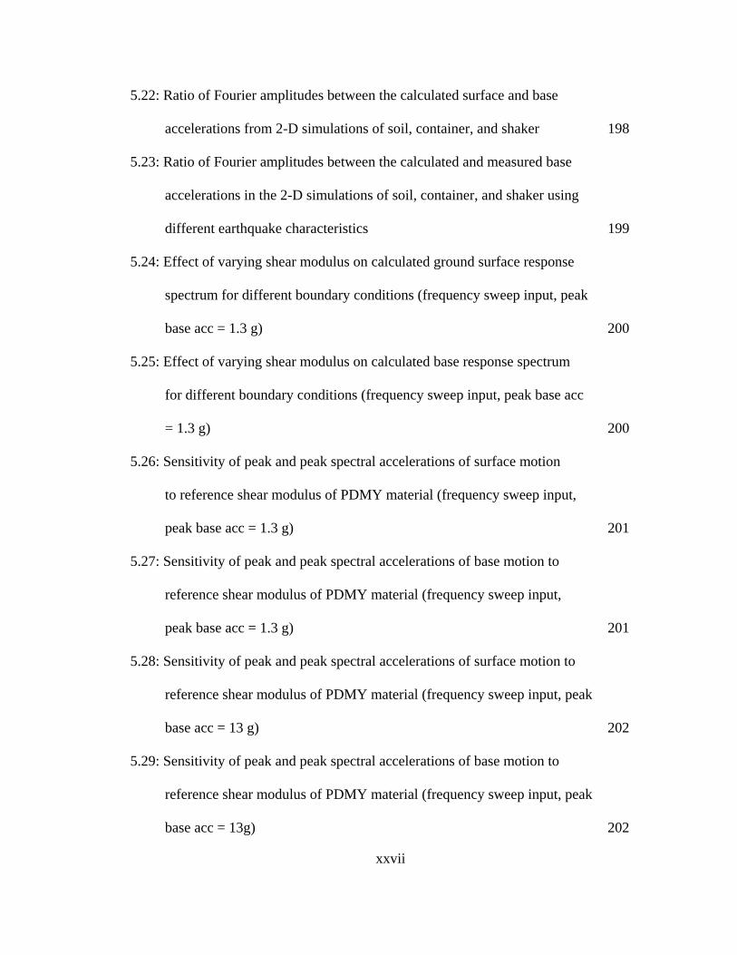
5.22: Ratio of Fourier amplitudes between the calculated surface and base
accelerations from 2-D simulations of soil, container, and shaker 198
5.23: Ratio of Fourier amplitudes between the calculated and measured base
accelerations in the 2-D simulations of soil, container, and shaker using
different earthquake characteristics 199
5.24: Effect of varying shear modulus on calculated ground surface response
spectrum for different boundary conditions (frequency sweep input, peak
base acc = 1.3 g) 200
5.25: Effect of varying shear modulus on calculated base response spectrum
for different boundary conditions (frequency sweep input, peak base acc
= 1.3 g) 200
5.26: Sensitivity of peak and peak spectral accelerations of surface motion
to reference shear modulus of PDMY material (frequency sweep input,
peak base acc = 1.3 g) 201
5.27: Sensitivity of peak and peak spectral accelerations of base motion to
reference shear modulus of PDMY material (frequency sweep input,
peak base acc = 1.3 g) 201
5.28: Sensitivity of peak and peak spectral accelerations of surface motion to
reference shear modulus of PDMY material (frequency sweep input, peak
base acc = 13 g) 202
5.29: Sensitivity of peak and peak spectral accelerations of base motion to
reference shear modulus of PDMY material (frequency sweep input, peak
base acc = 13g) 202
xxviii
Chapter 6
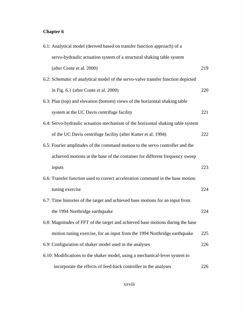
6.1: Analytical model (derived based on transfer function approach) of a
servo-hydraulic actuation system of a structural shaking table system
(after Conte et al. 2000) 219
6.2: Schematic of analytical model of the servo-valve transfer function depicted
in Fig. 6.1 (after Conte et al. 2000) 220
6.3: Plan (top) and elevation (bottom) views of the horizontal shaking table
system at the UC Davis centrifuge facility 221
6.4: Servo-hydraulic actuation mechanism of the horizontal shaking table system
of the UC Davis centrifuge facility (after Kutter et al. 1994) 222
6.5: Fourier amplitudes of the command motion to the servo controller and the
achieved motions at the base of the container for different frequency sweep
inputs 223
6.6: Transfer function used to correct acceleration command in the base motion
tuning exercise 224
6.7: Time histories of the target and achieved base motions for an input from
the 1994 Northridge earthquake 224
6.8: Magnitudes of FFT of the target and achieved base motions during the base
motion tuning exercise, for an input from the 1994 Northridge earthquake 225
6.9: Configuration of shaker model used in the analyses 226
6.10: Modifications to the shaker model, using a mechanical-lever system to
incorporate the effects of feed-back controller in the analyses 226
xxix
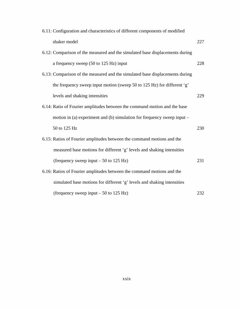
6.11: Configuration and characteristics of different components of modified
shaker model 227
6.12: Comparison of the measured and the simulated base displacements during
a frequency sweep (50 to 125 Hz) input 228
6.13: Comparison of the measured and the simulated base displacements during
the frequency sweep input motion (sweep 50 to 125 Hz) for different ‘g’
levels and shaking intensities 229
6.14: Ratio of Fourier amplitudes between the command motion and the base
motion in (a) experiment and (b) simulation for frequency sweep input –
50 to 125 Hz 230
6.15: Ratios of Fourier amplitudes between the command motions and the
measured base motions for different ‘g’ levels and shaking intensities
(frequency sweep input – 50 to 125 Hz) 231
6.16: Ratios of Fourier amplitudes between the command motions and the
simulated base motions for different ‘g’ levels and shaking intensities
(frequency sweep input – 50 to 125 Hz) 232
xxx
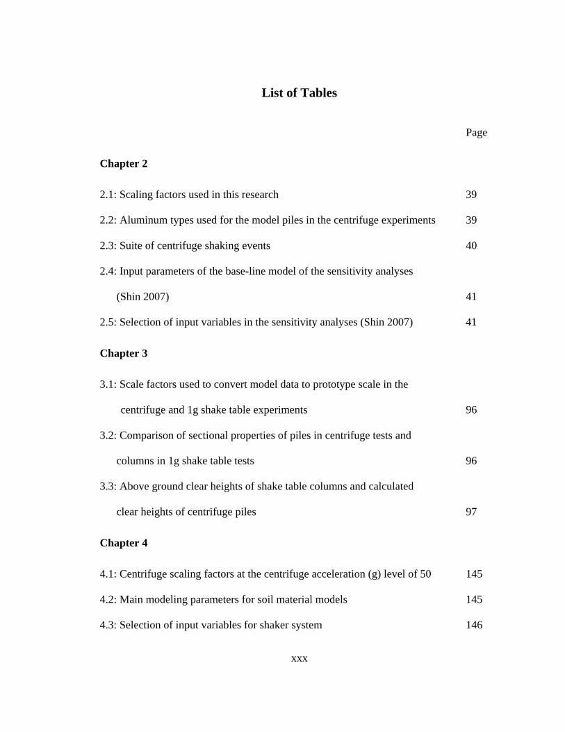
List of Tables
Page
Chapter 2
2.1: Scaling factors used in this research 39
2.2: Aluminum types used for the model piles in the centrifuge experiments 39
2.3: Suite of centrifuge shaking events 40
2.4: Input parameters of the base-line model of the sensitivity analyses
(Shin 2007) 41
2.5: Selection of input variables in the sensitivity analyses (Shin 2007) 41
Chapter 3
3.1: Scale factors used to convert model data to prototype scale in the
centrifuge and 1g shake table experiments 96
3.2: Comparison of sectional properties of piles in centrifuge tests and
columns in 1g shake table tests 96
3.3: Above ground clear heights of shake table columns and calculated
clear heights of centrifuge piles 97
Chapter 4
4.1: Centrifuge scaling factors at the centrifuge acceleration (g) level of 50 145
4.2: Main modeling parameters for soil material models 145
4.3: Selection of input variables for shaker system 146
xxxi
Chapter 5
5.1: Main modeling parameters for dry dense Nevada sand (Dr=80%) 180
5.2: Some design details of FSB2 model container 180
Chapter 1
Introduction
1.1 Background
1.1.1 Centrifuge testing of soil-foundation-bridge systems
Past earthquakes, particularly the 1989 Loma Prieta and 1994 Northridge
earthquakes in California, and the 1995 Kobe earthquake in Japan, have caused collapse
of, or severe damage to, a considerable number of major bridges that were designed for
seismic forces (Priestly et al. 1998, Fig. 1.1 and Fig. 1.2)). One major reason for the poor
performance relates to the complexities of the bridge structural and sub structural systems
as compared to other structures. Some of these complexities are wide variations in
structural types and configurations (bridge decks, columns/foundations, abutments, etc.),
variations in soil conditions along the length of a highway bridge (for example, presence
of potentially liquefied layers), and variations in ground motions (magnitude and phase
shift) along the length of the bridge (Fig. 1.3). In addition, soil-foundation-superstructure
interaction (SFSI) by which the soil interacts with the below ground and the above
ground portion of the bridge has an impact on the performance of the bridge during
earthquakes (Fig. 1.4). The impact of SFSI effects on the bridge system depend on the
ground motion and the nonlinear characteristics of the soil, foundation, and
superstructure. Accurate evaluations of SFSI effects are important to understand the
performance of a bridge under the seismic loading conditions.
1
In conjunction with lessons learnt from the case histories, researchers use
laboratory experiments to understand the performance of the key components of the
bridge system under the seismic loading conditions. In this context, dynamic centrifuge
modeling has been established as a powerful tool (Armstrong et al. 2008, Deng et al,
2008, etc.). Dynamic centrifuge modeling of bridge components designed with varying
soil profile characteristics, substructure/superstructure characteristics, loading protocols,
and detailed instrumentation is used to obtain physical data, gain insight into the
mechanisms involved, and perform parametric studies to calibrate numerical models. A
vast amount of research has been focused on the components of bridge systems to
understand the SFSI effects and to calibrate and validate computational models for SFSI
problems of bridge components (Wilson 1998, Abdoun et al. 2003, Chang et al, 2005,
Brandenberg 2005, Ugalde et al. 2007, etc). While a great amount of knowledge has been
gained about the component behavior of bridge components from these experiments, it is
important to perform experiments on soil-foundation-bridge systems to understand the
SFSI aspects of bridge systems and to validate the numerical model to predict bridge
system response. Kutter and Wilson (2006) describe the basic reasons for testing soil-
foundation-superstructure systems on the centrifuge as follows:
1) mechanisms of behavior that seem important for isolated foundations may not
come into play for soil-foundation-structure systems,
2) mechanisms of foundation behavior that are critical to the performance of the
structure may become apparent if the foundations and structures are tested as a
system, and
2

3) integrated numerical models that account for behavior of the soil, foundation and
structure need to be verified, especially for dynamic problems.
Cross-disciplinary interaction and collaboration between the geotechnical and the
structural engineers are essential for proper design of system experiments with the
realistic characteristics of substructure/superstructure, interpretation of these
experimental results, calibration of numerical models, and proper implementation of
gained knowledge into practice. In the past, limitations in experimental capabilities to
perform system experiments and lack of tools for effective means of collaborations pose
difficulties in conducting a collaborative research on the soil-foundations-bridge systems.
When the National Science Foundation’s George E. Brown, Jr. Network for
Earthquake Engineering Simulation (NEES) became operational in 2004, it provided
effective means for collaboration and facilitated a major improvement in research by
integrating experimental and computational simulations (http://nees.org). A larger scale
collaborative research project had been conducted to demonstrate the capabilities of
NEES for studying the effects SFSI on bridges and to conduct a comprehensive study of
SFSI effects by integrating analytical and experimental tools at multiple universities
(Wood et al. 2004, Fig. 1.5). One of the experimental components of this project
involved centrifuge modeling of soil-pile-bridge systems using the 9 m radius NEES
geotechnical centrifuge at the University of California, Davis. The collaborative research
on the centrifuge testing of soil-pile-bridge system is presented in this dissertation.
3
1.1.2 Soil – container – centrifuge shaker interaction
A typical centrifuge experiment involves different dynamic components (a
dynamic system) such as the test specimen, the soil model, the model container, the
shaking table, and its reaction mass (Fig. 1.6). All of the different components of
dynamic system, with their own resonant frequencies, interact with the soil model during
dynamic excitation, some absorbing energy and others allowing undesired modes to
affect the response observed in the experiment. This interaction between the soil model
and other components of the dynamic system (Fig. 1.7) might attenuate or exaggerate the
discrepancies in response of the experiment and the numerical simulation (Kutter 1994).
A fundamental question then arises: ‘How should we assess the quality of a comparison
between an experiment and a simulation results?’ To answer this fundamental question, it
would be essential to understand the sensitivity of simulation results (outputs) to
uncertainties in modeling parameters (inputs). In this context, it was hypothesized that the
“sensitivity of simulation results to uncertainties in modeling parameters depends on how
the boundary conditions are incorporated in the simulations”.
Qualitative assessment of the issues of dynamic interaction among soil model,
container, and shaker were addressed by many researchers in the past (Fiegel et al. 1994
and Narayanan 1999). However, a detailed numerical model to mathematically represent
the dynamics of the soil-model container-shaker system is necessary for comprehensive
understanding of this interaction and quantifying the effect of this interaction on the test
results.
4
1.2 Scope of the dissertation
This dissertation consists of the following four components: (1) A collaborative
research project involving centrifuge testing and numerical simulation of a soil-pile-
bridge system (2) A critical study to advance understanding the effects of using different
input motion boundary conditions on the sensitivity of numerical simulation results to
errors in material properties of a specimen tested on a shaking table (3) Numerical
simulations of a soil model tested on the centrifuge experiment accounting for soil-
container-shaker interaction, and (4) A first attempt to develop a numerical model of the
UC Davis servo-hydraulic centrifuge actuation system with a goal of predicting shaking
table response.
As mentioned earlier, the centrifuge experiments were part of a larger
collaborative project with the primary objectives of demonstrating the capabilities of the
network for earthquake engineering simulation (NEES) for studying the effects of soil-
foundation-structure interaction (SFSI) on bridges and conducting a comprehensive study
of SFSI effects by integrating analytical and experimental tools at multiple universities.
The centrifuge experiments complement the 1-g shake table and field shaker experiments
conducted at other universities. The design of test elements to facilitate direct
comparisons of experimental results between different experiments, to accounting for
different test boundary conditions and scaling laws for structural and geotechnical
modeling, was challenging and required cross-disciplinary interaction between
geotechnical and structural engineers.
The first part of this dissertation reports the lessons learnt from this collaborative
research both with respect to means for effective research collaboration and investigating
5
the SFSI effects by integrating experimental and analytical tools. It describes the
collaborative test design process, presents comparisons of experimental results in
different experiments, and reports the findings from the centrifuge testing of soil-pile-
bridge systems which involve realistic superstructure characteristics. In addition, the first
part of the dissertation describes the numerical simulations of the centrifuge experiments
performed by the collaborators from the University of Washington and compares the
simulation results with the experimental results. Understanding the discrepancies between
the results, in particular, the soil site response, in the centrifuge experiments and the
numerical simulations motivate the analyses presented in the second part of this
dissertation.
The second part of this dissertation is devoted to understand the importance of
more accurate treatment of the effects of soil-container-shaker interaction on the
numerical simulations of the centrifuge experiments. In this context, this dissertation
reports the findings from a series of numerical simulations of a hypothetical centrifuge
shaking table experiment that prove the hypothesis that “the sensitivity of simulation
results to uncertainties in modeling parameters depends on how the boundary conditions
are incorporated in the simulations”, the model development of a soil-container-
centrifuge shaker system including the modeling details of a servo-hydraulic centrifuge
actuation system , and the effects of dynamic interaction between the different
components of the centrifuge experimental system on the simulated site response results.
The centrifuge experiments produced unique data sets that span the disciplines of
geotechnical and structural engineering. This centrifuge test data and metadata and the
numerical model of the soil-container-shaker system are archived and curated in
6

NEEScentral data repository. These data archives are publically available at the
NEEScentral website (http://central.nees.org). The experimental data and the OpenSees
numerical models are available for others to use.
1.3 Organization of dissertation
The body of this dissertation is organized into seven chapters and an appendix. A
brief organizational summary of these chapters is given below.
Chapter 1 – Introduction
This chapter provides an overview of research and the scope and organizational
summary of the dissertation.
Chapter 2 – Collaborative research: Centrifuge testing of soil-pile-bridge systems
This chapter provides the summary of three dynamic centrifuge experiments on
soil-pile-bridge systems conducted at the UC Davis centrifuge facility. Details of these
experiments, including collaboration, experimental setup, representative test results,
comparisons with the complementary field shaker experiments, and a brief summary of
test data archives are presented. Numerical simulations of the centrifuge experiments,
performed by the collaborators from the University of Washington, are described and
compared with the experimental results.
Chapter 3 – Comparisons of centrifuge and 1-g shake table models of a pile supported
bridge structure
Comparisons of experimental results and the resolution of issues associated with
comparing physical models of a, two-span pile supported bridge structure tested at
different experimental facilities, at different scale, using different test boundary
conditions, and scaling laws are presented. A comparison between the system response of
7
the bridge model and the component response of individual bents during a series of
shaking events also presented in this chapter.
Chapter 4 – Modeling input motion boundary conditions for simulations of
geotechnical shaking table experiments
The effects of using different input motion boundary conditions on the sensitivity
of numerical simulation results to errors in material properties of a soil model tested on a
centrifuge shaking table are discussed using the numerical simulations of a hypothetical
centrifuge shaking table experiment involving a 1D soil column. The observation that the
sensitivity of simulation results to errors in input data depends on how the boundary
conditions are incorporated in the simulations, which increases the significance of proper
treatment of soil-container-shaker interaction on the simulations.
Chapter 5 – Numerical modeling of a soil - model container - centrifuge shaking table
system
Modeling of dynamics interaction of a soil-model container-centrifuge shaker
system is presented. Results from these simulations are compared with the experimental
results. Sensitivity studies are performed to propagate the uncertainties in modeling
parameters on the simulation results. The effects of soil-container-shaker interaction on
the sensitivities of the predicted site response results are discussed.
Chapter 6 – Towards developing a numerical model of a servo-hydraulic centrifuge
actuation system to predict shaking table response
The functioning of different components and the factors affecting the performance
of a servo-hydraulic actuation system are addressed in general. The actuation mechanism
of the UC Davis centrifuge horizontal shaking table system and the current procedures
8

used for input motion tuning in the experiments are outlined. An OpenSees numerical
model of this actuation system and the typical results from the numerical simulations are
presented. The predicted shaking table response results and the necessity for additional
work on this area are discussed.
Chapter 7 – Conclusions
This chapter provides a summary of the dissertation and its findings, and
recommendations for future work.
Appendix A – Centrifuge test and simulation data archives
This appendix provides details on the data archives of the centrifuge experiments
and the numerical simulations described in this dissertation, including the details of
collaborations with NEESit in the development of the NEEScentral data model and a
brief discussion about the current NEEScentral data model.
9
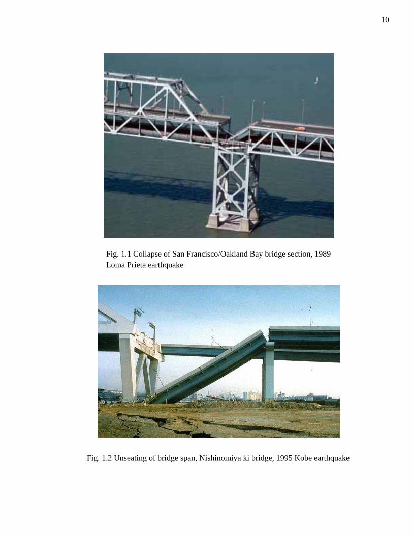
Fig. 1.1 Collapse of San Francisco/Oakland Bay bridge section, 1989 Loma Prieta earthquake
Fig. 1.2 Unseating of bridge span, Nishinomiya ki bridge, 1995 Kobe earthquake
10
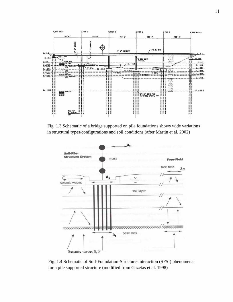
Fig. 1.3 Schematic of a bridge supported on pile foundations shows wide variations in structural types/configurations and soil conditions (after Martin et al. 2002)
Fig. 1.4 Schematic of Soil-Foundation-Structure-Interaction (SFSI) phenomena for a pile supported structure (modified from Gazetas et al. 1998)
11
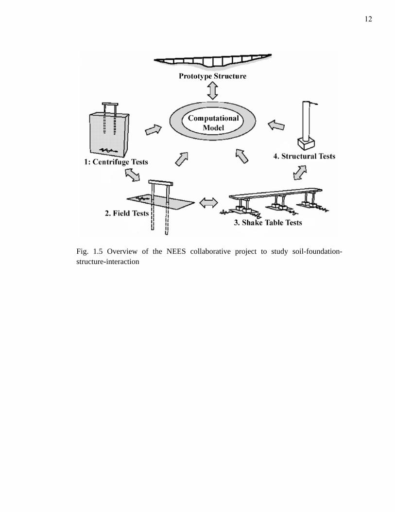
Fig. 1.5 Overview of the NEES collaborative project to study soil-foundation-structure-interaction
12
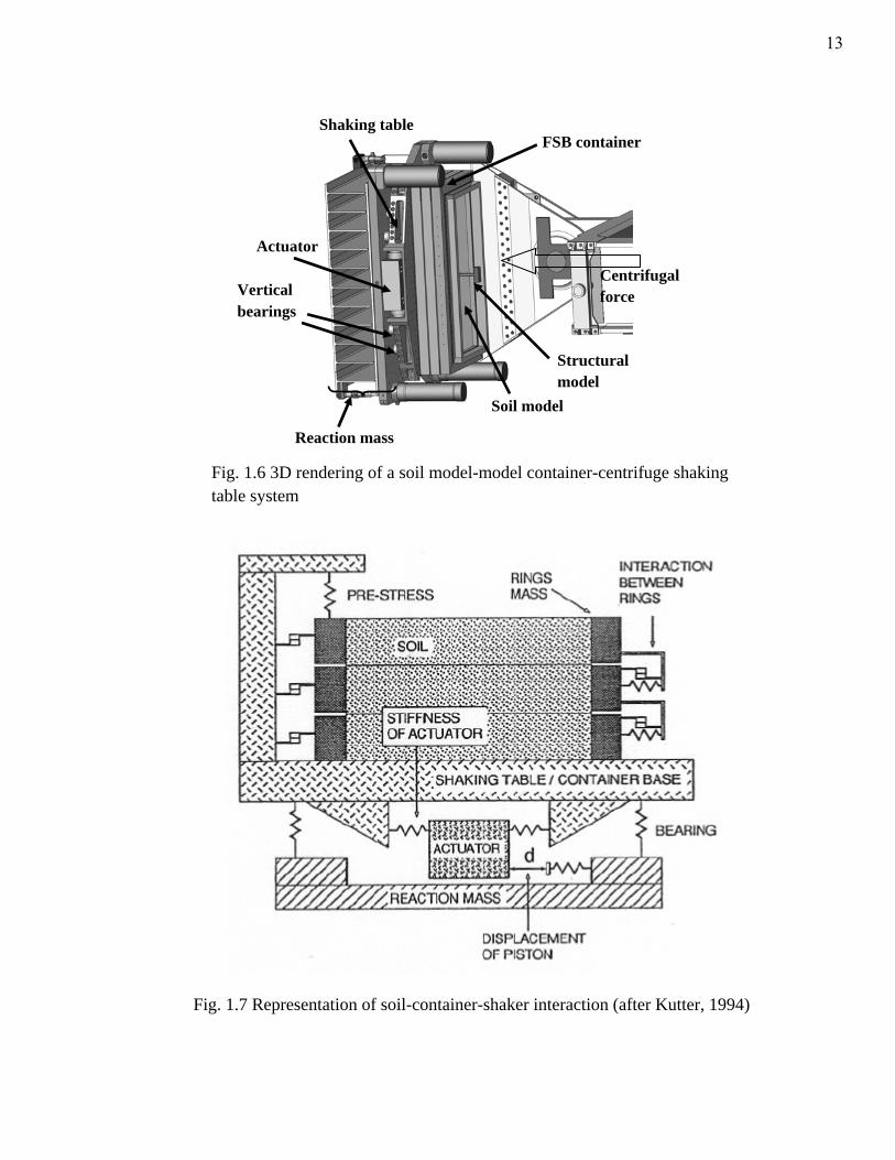
Fig. 1.6 3D rendering of a soil model-model container-centrifuge shaking table system
Vertical bearings
FSB container
Soil model
Structural model
Centrifugal force
Actuator
Shaking table
Reaction mass
Fig. 1.7 Representation of soil-container-shaker interaction (after Kutter, 1994)
13
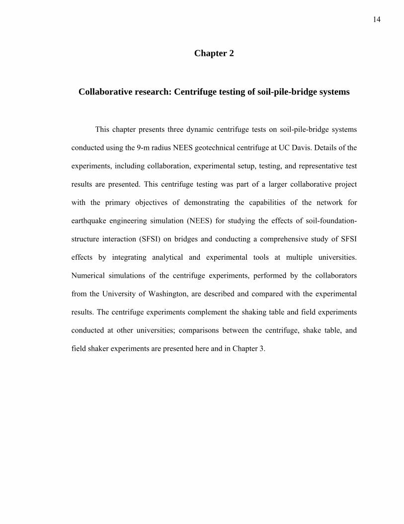
Chapter 2
Collaborative research: Centrifuge testing of soil-pile-bridge systems
This chapter presents three dynamic centrifuge tests on soil-pile-bridge systems
conducted using the 9-m radius NEES geotechnical centrifuge at UC Davis. Details of the
experiments, including collaboration, experimental setup, testing, and representative test
results are presented. This centrifuge testing was part of a larger collaborative project
with the primary objectives of demonstrating the capabilities of the network for
earthquake engineering simulation (NEES) for studying the effects of soil-foundation-
structure interaction (SFSI) on bridges and conducting a comprehensive study of SFSI
effects by integrating analytical and experimental tools at multiple universities.
Numerical simulations of the centrifuge experiments, performed by the collaborators
from the University of Washington, are described and compared with the experimental
results. The centrifuge experiments complement the shaking table and field experiments
conducted at other universities; comparisons between the centrifuge, shake table, and
field shaker experiments are presented here and in Chapter 3.
14
2.1 NEES collaborative research project to study SFSI
The primary objectives of the collaborative research were: (a) to demonstrate the
Network for earthquake Engineering Simulation (NEES) for studying soil-foundation-
structure-interaction (SFSI) (Wood et al. 2004), (b) to conduct a comprehensive study of
SFSI by integrating analytical and experimental tools at multiple universities.
Experimental studies were conducted at four sites across the United States (Fig. 2.1): (a)
1-g shake table experiments at the University of Nevada, Reno (b) centrifuge tests at UC
Davis (c) field tests using the large shakers at the University of Texas, Austin, and (d)
Quasi-static structural component testing at Purdue University. The team of researchers
also included numerical analysts from the University of Washington, the University of
California, Berkeley, and the University of California, Davis, as well as a team of
researchers from Kansas University to coordinate archiving and sharing of data, and an
education and outreach component at San Jose State University. The prototype for the
experimental studies (shown in Fig. 2.2) was a two-span frame of a cast-in-place post-
tensioned reinforced concrete box girder bridge. The span lengths were 120 ft (37 m), and
the substructure was composed of 4 ft (1.2 m) diameter 2-column piers on extended pile
foundations. Due to the size and the complexity of the prototype system, it was
impossible to test a single physical model and reproduce all key aspects of the system
performance. Therefore, the tests at various facilities were intended to provide a means
for comprehensive validation of numerical procedures for analyzing the behavior of a
bridge supported on piles. Details of these different experiments are briefly described
below.
15
2.1.1 Field tests
The field test specimens consisted of two, quarter scale, two column bridge bents
which were constructed at the Capitol Aggregates test site (Kurtuluş et al. 2005). Three
different types of dynamic tests were conducted on these test specimens. Initially, the
specimens were stuck with a modal hammer to induce low-amplitude, free vibration
response. Then the large NEES mobile shaker, T-Rex, was used to induce harmonic
vibrations in the test specimens by exciting the surface of the ground (see Fig. 2.3).
Finally, the hydraulic shaker from the small NEES mobile shaker, Thumper, was attached
to the bent cap and used to excite the specimens harmonically (shown in Fig. 2.4). These
field tests were designed to provide a means of understanding the linear response of the
complete soil-foundation-super structure system during dynamic loading in insitu test
conditions. Further details on these experiments can be found in Black (2005) and
Agarwal et al 2006.
2.1.2 Structural component tests
The structural component test consisted of fixed-base, quarter-scale and half-scale
single shafts and two-column bridge bents (shown in Fig. 2.5). The purposes of these
experiments were to determine the effects of reinforcement detailing, size, and shear span
to depth ratio on the cyclic response of bridge columns. The complete details on these
experiments can be found in Makido (2007).
2.1.3 1-g shake table experiment
The shaking table experiment consisted of a quarter scale model of the two-span
prototype bridge section (shown in Fig. 2.6). The testing was performed in two phases.
16
During low amplitude tests, incoherent, bidirectional ground motion was used to excite
the specimen. Coherent ground motion in the transverse direction of the bridge was used
during the larger amplitude tests. Some additional details of this experiment including the
test set up and comparisons with the complementary centrifuge test model are presented
in Chapter 3 of this dissertation. The comprehensive details of this test program are
provided in Johnson et al. 2006.
2.1.4 Centrifuge experiments
The centrifuge test program included 1/52 scale models of single-pile bents, two-
pile bents and a two-span section of the prototype bridge. Aluminum tubes were used to
model the column and the aluminum blocks were used to represent superstructures (see
Fig. 2.7). Dry Nevada sand, placed at a relative density of 80% in a flexible shear beam
model container, was used to model soil in the experiments. Details of these centrifuge
experiments are given in the following sections.
2.2 Centrifuge test program
2.2.1 Concept of the geotechnical centrifuge modeling
Geotechnical centrifuge modeling has been established as a powerful tool to
investigate the seismic behavior of soil-structure systems. The concept of the
geotechnical centrifuge modeling is described at the web site of the Center for
Geotechnical Modeling, UC Davis as follows: “Geotechnical materials such as soil and
rock have nonlinear mechanical properties that depend on the effective confining stress
and stress history. The centrifuge applies an increased "gravitational" acceleration to
physical models in order to produce identical self-weight stresses in the model and
17
prototype. The one to one scaling of stress enhances the similarity of geotechnical models
and makes it possible to obtain accurate data to help solve complex problems such as
earthquake-induced liquefaction, soil-structure interaction and underground transport of
pollutants. Centrifuge model testing provides data to improve our understanding of basic
mechanisms of deformation and failure and provides benchmarks useful for verification
of numerical models” (http://cgm.engineering.ucdavis.edu/). A set of scaling laws are
used to convert model-scale data to appropriate prototype-scale data. The details on these
scaling laws can be found in (Schofield, 1981 and Kutter, 1992). All the centrifuge
experiments were performed at 52g centrifuge acceleration. All the results presented in
this chapter are in prototype scale unless otherwise specified. Table 2.1 lists the scale
factors which were used to convert model quantities to prototype scales.
2.2.2 Model configurations
A series of three centrifuge test series was constructed and tested. The objectives
of these experiments were to complement the field and laboratory test conducted
elsewhere and to provide insight into geotechnical-oriented aspects of the soil-pile-bridge
systems. A brief summary of these three experiments is presented below.
2.2.2.1 Centrifuge test series MIL01
This test series included a scale model of a two-bay prototype bridge structure
with the sloping ground conditions that were assumed to exist at the site of the prototype
bridge structure. Due to the sloping ground, the two bays were supported by three bents,
but the clear height between the soil and bridge deck was different for each bent. The
centrifuge test package also included an independent two-pile bent corresponding to
18
medium-height bent in the prototype structure, another independent medium height bent
which is fixed at the bridge deck and a pile cap at the ground surface level, and a single
pile corresponding to pile in the tallest bent. The model layout of the MIL01 test series,
including the details of the structural models are shown in Fig. 2.8 and in Fig. 2.9. The
1/52 scale model of the two-bay prototype bridge structure in this centrifuge test series
complements the ¼ scale model of the prototype bridge structure tested in the 1-g shake
table facility at the University of Nevada, Reno.
2.2.2.2 Centrifuge test series MIL02
This test series included pile structures that allow investigation of the response of
two-pile bents. The model included four identical two-pile bents oriented at angles of 0,
30, 60, and 90 degrees to the direction of shaking, and a single pile supporting a weight
equal to the weights supported by the individual piles in the two-pile bents (depicted in
Fig. 2.10). As shown in Fig. 2.10, the above ground clear height was 75 mm (in model
scale) for all the bents and the single pile. This test series experiments provided
experimental data on the response of a two-pile bent to motions coming from different
angles in which the pile bent would have different relative flexural and axial response.
This data complements data obtained from quarter scale field tests performed at
University of Texas at Austin, in which the vibration source (T-Rex) was moved to
different locations relative to the two-pile bent.
2.2.2.3 Centrifuge test series MIL03
This test series included pile structures that allow investigation of the dynamic
response of two-pile bents and single piles (4 two-pile bents and 3 single piles). The
model layout of the MIL03 test series and the 3-D rendering of the model set-up are
19
shown in Fig. 2.11. The configurations of structural models used in the experiment are
depicted in Fig. 2.12. As shown in above figures, the longer axes of the two-pile bents 2-
LL-Hy and 2-SS-Hy were oriented in the direction of shaking and those of bents 2-LS-Lt
and 2-LS-Hy were oriented 90 degrees to the direction of shaking. The bents 2-LL-Hy
and 2-SS-Hy were identical above the ground surface; however, their pile embedment
lengths were different. The bent 2-LL-Hy had an embedment length of 12.1D and the
bent 2-SS-Hy had an embedment length of 5D, where D is outer diameter of piles (22.71
mm in model scale). The bents 2-LS-Lt and 2-LS-Hy were identical below the ground
surface. Each of the above bents was supported by a longer pile (12.1D embedment) and
a shorter pile (5D embedment). In this case, it was expected to induce torsional response
in the bent by supporting one side on shorter pile and the other on a longer pile. An extra
mass attached to the bent 2-LS-Hy to support 1.5 times “heavier” mass than” lighter”
bent 2-LS-Lt. The three single piles (1-S, 1-M, and 1-L) were designed to have different
embedment lengths, the embedment lengths of these piles were 5D, 7.5D, and 12.1D,
respectively. The primary purpose of this experiment was to provide experimental data to
the collaborators in the University of Washington to validate their OpenSees
computational models of soil-pile-superstructure systems.
2.2.3 Design of structural models
The design of the centrifuge model structures was based on the dimensions and
properties of the columns, bents, and deck from the 1-g shaking table experiment. All
model piles were made of 6061-T4 (E=68.5 GPa; yield strength=130 MPa) and 6061-T6
(E=68.5 GPa; yield strength=255 MPa) aluminum tubes of 19.05 mm diameter (0.991 m
prototype) and a wall thickness of 0.889 mm (0.046 m prototype). Table 2.2 lists the
20

aluminum type used for the model piles in all three centrifuge experiments. Strain gages
were affixed to piles and piles were covered with plastic shrink-wrap. The outer diameter
of composite pile was 22.71 mm (1.181 m in prototype scale). The model pile used in the
MIL01 test series were reused in other two centrifuge experiments. All the bent blocks
were made of 6061-T6 aluminum (E=68.5 GPa; yield strength=255 MPa). Further details
of the design of structures and the dimensions and properties of the model structures can
be found in the centrifuge test series data report Ilankatharan et al. 2005.
2.2.4 Model preparation and instrumentation
The soil chosen for the centrifuge test was dry Nevada sand (80% relative
density). The relative density of Nevada sand was picked to reasonably match the low-
strain shear wave velocity profile of the Capitol Aggregates test site, Austin. Fig. 2.13
shows the shear wave velocity profile of the test site and the 80% relative density Nevada
sand calculated based on the data available in the literature (Arulnathan et al. 2000). The
field experiments are conducted under 1-g condition; while the centrifuge experiments
are conducted under increased gravity condition. Therefore the scaling is complicated
between two experiments, since we have different soils and different confining pressures
in the field and the centrifuge experiments. The field test model-bent has an embedment
length of 3.6 m (12 times the diameter of the column) and the centrifuge model bent has
embedment length of 14 m (approximately 12 times the diameter of the pile). It was
considered that the discrepancies between the shear-wave velocity profiles shown in Fig.
2.13 might counterbalance the differences in strength of soil due to the differences in
vertical stress fields in the field and the centrifuge experiments (i.e., vertical stress fields
21

are off by a factor of 4 approximately). Based on this assumption, it was considered that
the mismatch of shear wave velocity profiles in Fig. 2.13 is acceptable.
The dense sand was placed by dry pluviation. When the soil was 50 mm below
the final soil profile, accelerometers were attached on the piles and the piles were
attached to the bent caps and pushed in pairs into the soil by hand about half way. A
hammer was then used to drive the bents to the desired depth. A bubble level was used to
ensure that piles are driven in vertically. Then bent caps were removed and the barrel
pluviator was used to place top soil layer to produce soil around and above the
accelerometers to produce the final soil profile.
The model was heavily instrumented with accelerometers, linear potentiometers,
and strain gage bridges to measure the translation, rotation and bending response of the
foundations, columns, and bent cap (see Fig. 2.14). Additional accelerometers were
embedded in the soil to measure soil response during dynamic loading. Vertical linear
potentiometers were used to measure ground surface settlement during shaking. In
addition to the above conventional instrumentation, models were instrumented with high
speed video cameras and MEMS accelerometers using the UC Davis high-speed wireless
data acquisition system (shown in Fig. 2.15). Performance of the newly developed UC
Davis high-speed wireless data acquisition system was evaluated in these centrifuge test
series as it was first introduced for centrifuge test applications at the UC Davis centrifuge
facility. Fig. 2.16 presents a comparison of data recorded with traditional wired data
acquisition system and the wireless data acquisition (transducers were placed at nearly
identical locations for direct comparison).
22
2.2.5 Ground motion protocols
Each centrifuge models was subjected to a series of shaking events, beginning
with very low-level shaking events to characterize the low-strain response of the soil and
soil-pile-superstructure systems and progressive to very strong motions with peak base
accelerations of up to 0.75g. Input base motions included step displacement waves,
frequency sweeps and scaled versions of recorded earthquake motion during the 1994
Northridge Earthquake at the CDMG station 24389, Century City LACC North, 090. Fig.
2.17 shows the time histories and response spectra (5% damping) of some of the input
motions used in the experiments. The entire shaking schedule is shown in Table 2.3.
2.3 Representative results from centrifuge experiments
Representative results from some selected centrifuge shaking events are presented
in this section. The complete set of centrifuge test data and metadata is presented in the
test series data report Ilankatharan et al. (2005), which is archived in NEEScentral data
repository (http://central.nees.org).
2.3.1 Soil site response
Fig. 2.18 presents typical site response results characterized by a vertical array of
horizontal accelerometers placed in the middle of the model container. These measured
soil site response results were used to verify the numerical simulations of centrifuge
experiments. Comparisons between the measured and predicted (using 1-D shear beam
simulation model) site response results are presented later in this chapter.
23
2.3.2 Horizontal accelerations
Time histories and response spectra (5% damping) of recorded horizontal
accelerations at different locations of model during a centrifuge shaking event is shown
in Fig. 2.19. As shown in Fig. 2.19, the measured free-field soil motion at 2.5m below the
ground surface shows greater amplification (with respect to the measured base motion) in
the intermediate frequency range compare to the higher frequency (short period) range.
Measured pile motion (from an accelerometer directly attached to pile) at 2.5 m below
ground surface is nearly the same as the measured free-field soil motion at that depth.
This observation indicates that the kinematic soil-pile interaction effects (Gazetas et al.
1998) are not very significant for this problem. As expected, the superstructure is not
excited by the higher frequency content of the base motion and shows a high response
peak in the lower frequency (long period) range.
2.3.3 Vertical accelerations
Fig. 2.20 presents the measured vertical motions at the container base and at 2.6
m (in prototype scale) below the ground surface at both ends of the container. It is clear
from Fig. 2.20 that the time histories of measured vertical accelerations are 180 degrees
out of phase, show rocking response of the container. In addition, for this medium-level
shaking event, the measured peak vertical base motion is 42% of the peak base
(horizontal) motion and the measured peak vertical soil motion is 75% of the peak base
motion.
24
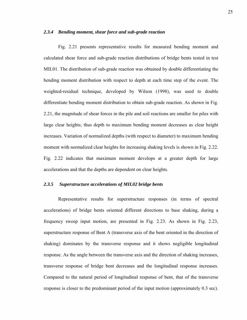
2.3.4 Bending moment, shear force and sub-grade reaction
Fig. 2.21 presents representative results for measured bending moment and
calculated shear force and sub-grade reaction distributions of bridge bents tested in test
MIL01. The distribution of sub-grade reaction was obtained by double differentiating the
bending moment distribution with respect to depth at each time step of the event. The
weighted-residual technique, developed by Wilson (1998), was used to double
differentiate bending moment distribution to obtain sub-grade reaction. As shown in Fig.
2.21, the magnitude of shear forces in the pile and soil reactions are smaller for piles with
large clear heights; thus depth to maximum bending moment decreases as clear height
increases. Variation of normalized depths (with respect to diameter) to maximum bending
moment with normalized clear heights for increasing shaking levels is shown in Fig. 2.22.
Fig. 2.22 indicates that maximum moment develops at a greater depth for large
accelerations and that the depths are dependent on clear heights.
2.3.5 Superstructure accelerations of MIL02 bridge bents
Representative results for superstructure responses (in terms of spectral
accelerations) of bridge bents oriented different directions to base shaking, during a
frequency sweep input motion, are presented in Fig. 2.23. As shown in Fig. 2.23,
superstructure response of Bent A (transverse axis of the bent oriented in the direction of
shaking) dominates by the transverse response and it shows negligible longitudinal
response. As the angle between the transverse axis and the direction of shaking increases,
transverse response of bridge bent decreases and the longitudinal response increases.
Compared to the natural period of longitudinal response of bent, that of the transverse
response is closer to the predominant period of the input motion (approximately 0.3 sec).
25
The large difference between the peaks of transverse response of Bent A and the
longitudinal response of Bent D may be attributable to the close proximity of natural
period of bridge bent (for transverse response) to the predominant period of the input
motion.
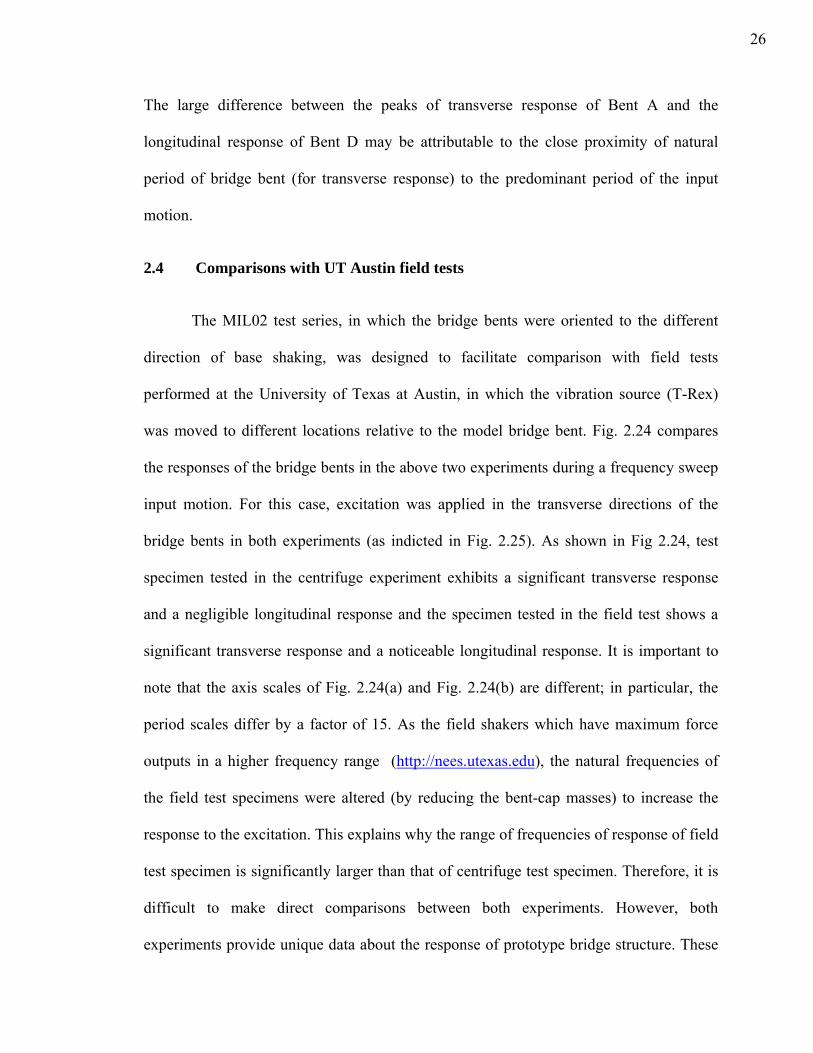
2.4 Comparisons with UT Austin field tests
The MIL02 test series, in which the bridge bents were oriented to the different
direction of base shaking, was designed to facilitate comparison with field tests
performed at the University of Texas at Austin, in which the vibration source (T-Rex)
was moved to different locations relative to the model bridge bent. Fig. 2.24 compares
the responses of the bridge bents in the above two experiments during a frequency sweep
input motion. For this case, excitation was applied in the transverse directions of the
bridge bents in both experiments (as indicted in Fig. 2.25). As shown in Fig 2.24, test
specimen tested in the centrifuge experiment exhibits a significant transverse response
and a negligible longitudinal response and the specimen tested in the field test shows a
significant transverse response and a noticeable longitudinal response. It is important to
note that the axis scales of Fig. 2.24(a) and Fig. 2.24(b) are different; in particular, the
period scales differ by a factor of 15. As the field shakers which have maximum force
outputs in a higher frequency range (http://nees.utexas.edu), the natural frequencies of
the field test specimens were altered (by reducing the bent-cap masses) to increase the
response to the excitation. This explains why the range of frequencies of response of field
test specimen is significantly larger than that of centrifuge test specimen. Therefore, it is
difficult to make direct comparisons between both experiments. However, both
experiments provide unique data about the response of prototype bridge structure. These
26
unique data sets were used to calibrate the simulation methods for seismic soil-
foundation-structure interaction problems (Shin 2007 and Jie 2007).
2.5 Simulations of centrifuge models
Numerical simulations of the centrifuge experiments were performed, using
OpenSees (Open System for Earthquake Engineering Simulation,
http://opensees.berkeley.edu/index.php), by the collaborators from the University of
Washington (Shin et al, 2006 and Shin 2007). A brief outline of these simulation models
and some of the comparisons of simulation results with the experimental results are
presented in the following sections.
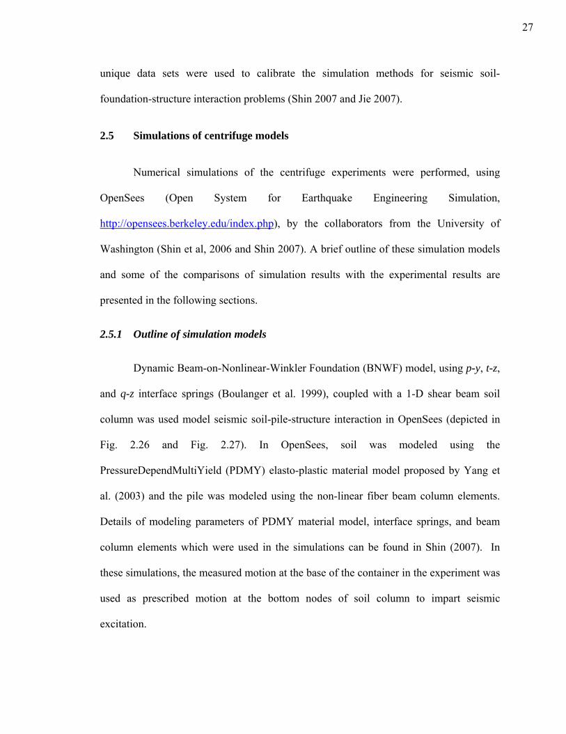
2.5.1 Outline of simulation models
Dynamic Beam-on-Nonlinear-Winkler Foundation (BNWF) model, using p-y, t-z,
and q-z interface springs (Boulanger et al. 1999), coupled with a 1-D shear beam soil
column was used model seismic soil-pile-structure interaction in OpenSees (depicted in
Fig. 2.26 and Fig. 2.27). In OpenSees, soil was modeled using the
PressureDependMultiYield (PDMY) elasto-plastic material model proposed by Yang et
al. (2003) and the pile was modeled using the non-linear fiber beam column elements.
Details of modeling parameters of PDMY material model, interface springs, and beam
column elements which were used in the simulations can be found in Shin (2007). In
these simulations, the measured motion at the base of the container in the experiment was
used as prescribed motion at the bottom nodes of soil column to impart seismic
excitation.
27
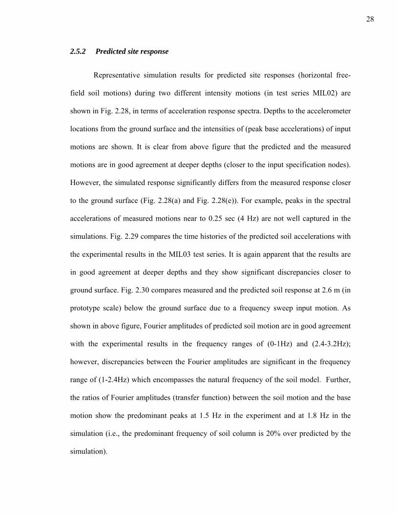
2.5.2 Predicted site response
Representative simulation results for predicted site responses (horizontal free-
field soil motions) during two different intensity motions (in test series MIL02) are
shown in Fig. 2.28, in terms of acceleration response spectra. Depths to the accelerometer
locations from the ground surface and the intensities of (peak base accelerations) of input
motions are shown. It is clear from above figure that the predicted and the measured
motions are in good agreement at deeper depths (closer to the input specification nodes).
However, the simulated response significantly differs from the measured response closer
to the ground surface (Fig. 2.28(a) and Fig. 2.28(e)). For example, peaks in the spectral
accelerations of measured motions near to 0.25 sec (4 Hz) are not well captured in the
simulations. Fig. 2.29 compares the time histories of the predicted soil accelerations with
the experimental results in the MIL03 test series. It is again apparent that the results are
in good agreement at deeper depths and they show significant discrepancies closer to
ground surface. Fig. 2.30 compares measured and the predicted soil response at 2.6 m (in
prototype scale) below the ground surface due to a frequency sweep input motion. As
shown in above figure, Fourier amplitudes of predicted soil motion are in good agreement
with the experimental results in the frequency ranges of (0-1Hz) and (2.4-3.2Hz);
however, discrepancies between the Fourier amplitudes are significant in the frequency
range of (1-2.4Hz) which encompasses the natural frequency of the soil model. Further,
the ratios of Fourier amplitudes (transfer function) between the soil motion and the base
motion show the predominant peaks at 1.5 Hz in the experiment and at 1.8 Hz in the
simulation (i.e., the predominant frequency of soil column is 20% over predicted by the
simulation).
28
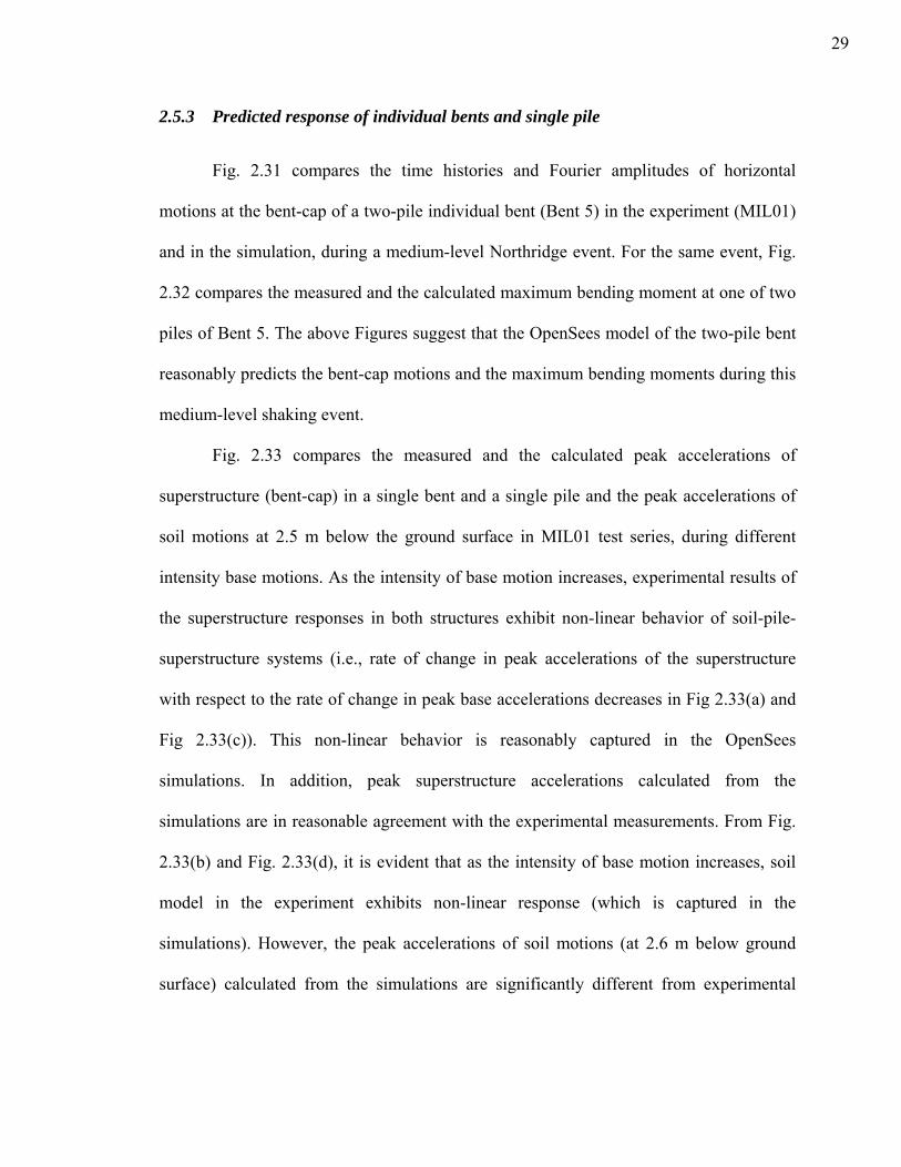
2.5.3 Predicted response of individual bents and single pile
Fig. 2.31 compares the time histories and Fourier amplitudes of horizontal
motions at the bent-cap of a two-pile individual bent (Bent 5) in the experiment (MIL01)
and in the simulation, during a medium-level Northridge event. For the same event, Fig.
2.32 compares the measured and the calculated maximum bending moment at one of two
piles of Bent 5. The above Figures suggest that the OpenSees model of the two-pile bent
reasonably predicts the bent-cap motions and the maximum bending moments during this
medium-level shaking event.
Fig. 2.33 compares the measured and the calculated peak accelerations of
superstructure (bent-cap) in a single bent and a single pile and the peak accelerations of
soil motions at 2.5 m below the ground surface in MIL01 test series, during different
intensity base motions. As the intensity of base motion increases, experimental results of
the superstructure responses in both structures exhibit non-linear behavior of soil-pile-
superstructure systems (i.e., rate of change in peak accelerations of the superstructure
with respect to the rate of change in peak base accelerations decreases in Fig 2.33(a) and
Fig 2.33(c)). This non-linear behavior is reasonably captured in the OpenSees
simulations. In addition, peak superstructure accelerations calculated from the
simulations are in reasonable agreement with the experimental measurements. From Fig.
2.33(b) and Fig. 2.33(d), it is evident that as the intensity of base motion increases, soil
model in the experiment exhibits non-linear response (which is captured in the
simulations). However, the peak accelerations of soil motions (at 2.6 m below ground
surface) calculated from the simulations are significantly different from experimental
29
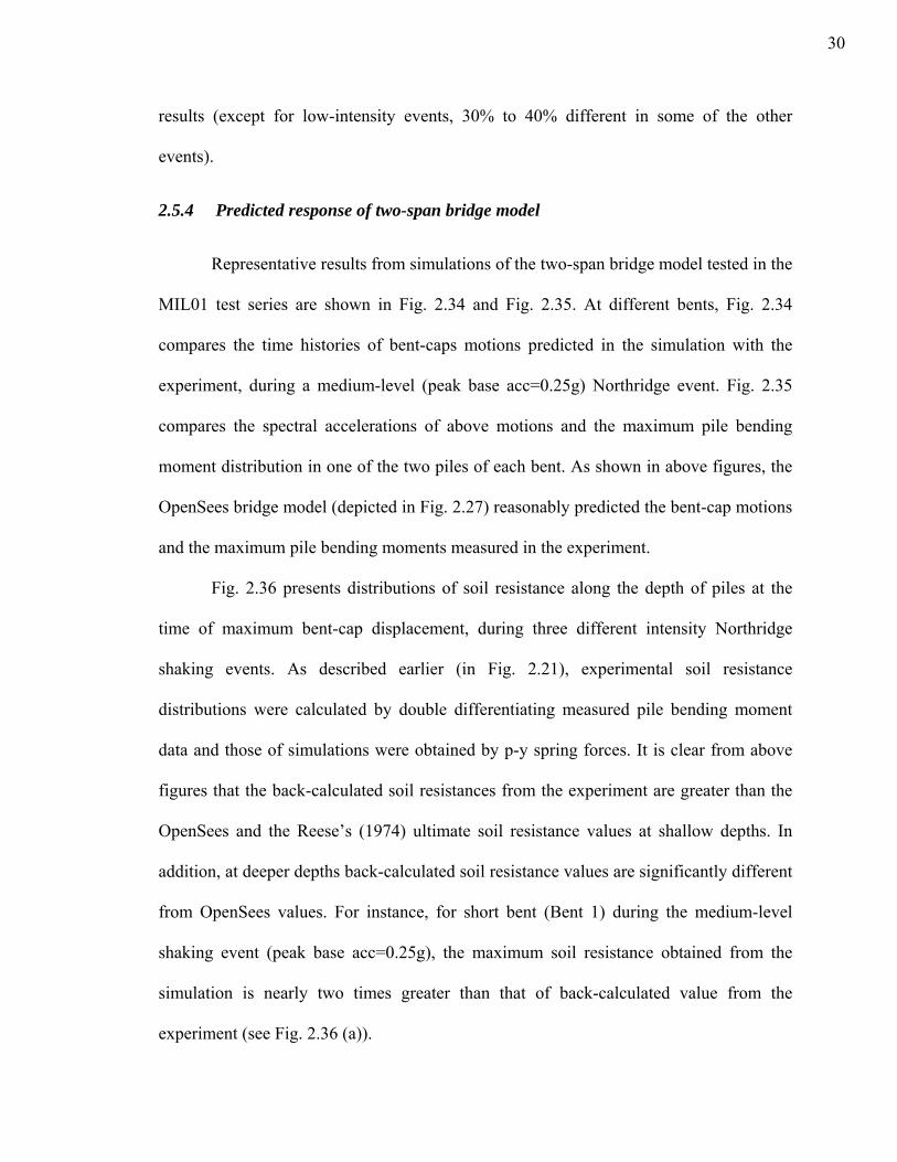
results (except for low-intensity events, 30% to 40% different in some of the other
events).
2.5.4 Predicted response of two-span bridge model
Representative results from simulations of the two-span bridge model tested in the
MIL01 test series are shown in Fig. 2.34 and Fig. 2.35. At different bents, Fig. 2.34
compares the time histories of bent-caps motions predicted in the simulation with the
experiment, during a medium-level (peak base acc=0.25g) Northridge event. Fig. 2.35
compares the spectral accelerations of above motions and the maximum pile bending
moment distribution in one of the two piles of each bent. As shown in above figures, the
OpenSees bridge model (depicted in Fig. 2.27) reasonably predicted the bent-cap motions
and the maximum pile bending moments measured in the experiment.
Fig. 2.36 presents distributions of soil resistance along the depth of piles at the
time of maximum bent-cap displacement, during three different intensity Northridge
shaking events. As described earlier (in Fig. 2.21), experimental soil resistance
distributions were calculated by double differentiating measured pile bending moment
data and those of simulations were obtained by p-y spring forces. It is clear from above
figures that the back-calculated soil resistances from the experiment are greater than the
OpenSees and the Reese’s (1974) ultimate soil resistance values at shallow depths. In
addition, at deeper depths back-calculated soil resistance values are significantly different
from OpenSees values. For instance, for short bent (Bent 1) during the medium-level
shaking event (peak base acc=0.25g), the maximum soil resistance obtained from the
simulation is nearly two times greater than that of back-calculated value from the
experiment (see Fig. 2.36 (a)).
30
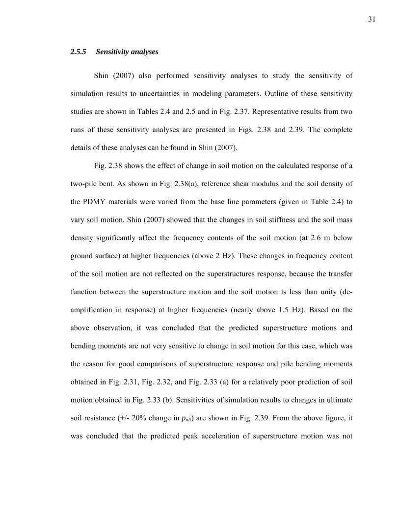
2.5.5 Sensitivity analyses
Shin (2007) also performed sensitivity analyses to study the sensitivity of
simulation results to uncertainties in modeling parameters. Outline of these sensitivity
studies are shown in Tables 2.4 and 2.5 and in Fig. 2.37. Representative results from two
runs of these sensitivity analyses are presented in Figs. 2.38 and 2.39. The complete
details of these analyses can be found in Shin (2007).
Fig. 2.38 shows the effect of change in soil motion on the calculated response of a
two-pile bent. As shown in Fig. 2.38(a), reference shear modulus and the soil density of
the PDMY materials were varied from the base line parameters (given in Table 2.4) to
vary soil motion. Shin (2007) showed that the changes in soil stiffness and the soil mass
density significantly affect the frequency contents of the soil motion (at 2.6 m below
ground surface) at higher frequencies (above 2 Hz). These changes in frequency content
of the soil motion are not reflected on the superstructures response, because the transfer
function between the superstructure motion and the soil motion is less than unity (de-
amplification in response) at higher frequencies (nearly above 1.5 Hz). Based on the
above observation, it was concluded that the predicted superstructure motions and
bending moments are not very sensitive to change in soil motion for this case, which was
the reason for good comparisons of superstructure response and pile bending moments
obtained in Fig. 2.31, Fig. 2.32, and Fig. 2.33 (a) for a relatively poor prediction of soil
motion obtained in Fig. 2.33 (b). Sensitivities of simulation results to changes in ultimate
soil resistance (+/- 20% change in pult) are shown in Fig. 2.39. From the above figure, it
was concluded that the predicted peak acceleration of superstructure motion was not
31

affected by the changes in pult and the predicted pile bending moment distribution was
slightly affected by the changes in pult.
2.5.6 Simulations of MIL02 and MIL03 test series
Numerical modeling of bridge bents tested in MIL02 and MIL03 test series also
performed by the collaborators from the University of Washington. As described earlier,
MIL02 test series involved individual two-pile bents oriented different directions to the
base shaking and the MIL03 test series involved individual two-pile bents and single-pile
bents with different embedment lengths, bent-cap masses, and structural configurations.
Details of these simulations including the modeling strategies, modeling parameters, and
the comparisons of simulation results with experimental results are presented in Shin et
al. (2006) and Shin (2007).
2.6 Simulation of the prototype bridge structure
Computational simulations of the prototype bridge structure (depicted in Fig. 2.2)
were performed by the collaborators from the UC Davis, UC Berkeley, and the
University of Washington. The unique data sets obtained from all four experiments (in
Fig. 2.1) were used in the model developments, verifications and validations of these
simulations. 3-D finite element model of one of the simulations of the prototype soil-pile-
bridge system is depicted in Fig. 2.40. Comprehensive details of these simulations can be
found in Jie (2007), Ranf (2007), and Dryden (2008).
32
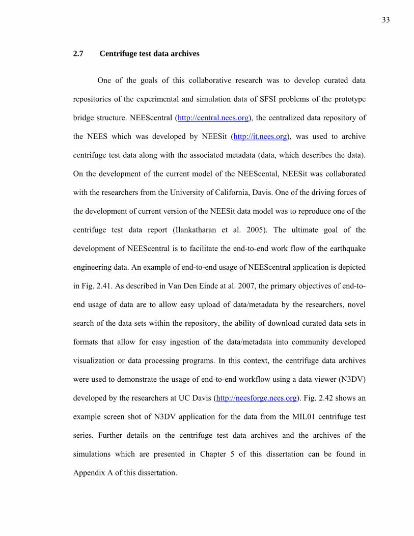
2.7 Centrifuge test data archives
One of the goals of this collaborative research was to develop curated data
repositories of the experimental and simulation data of SFSI problems of the prototype
bridge structure. NEEScentral (http://central.nees.org), the centralized data repository of
the NEES which was developed by NEESit (http://it.nees.org), was used to archive
centrifuge test data along with the associated metadata (data, which describes the data).
On the development of the current model of the NEEScental, NEESit was collaborated
with the researchers from the University of California, Davis. One of the driving forces of
the development of current version of the NEESit data model was to reproduce one of the
centrifuge test data report (Ilankatharan et al. 2005). The ultimate goal of the
development of NEEScentral is to facilitate the end-to-end work flow of the earthquake
engineering data. An example of end-to-end usage of NEEScentral application is depicted
in Fig. 2.41. As described in Van Den Einde at al. 2007, the primary objectives of end-to-
end usage of data are to allow easy upload of data/metadata by the researchers, novel
search of the data sets within the repository, the ability of download curated data sets in
formats that allow for easy ingestion of the data/metadata into community developed
visualization or data processing programs. In this context, the centrifuge data archives
were used to demonstrate the usage of end-to-end workflow using a data viewer (N3DV)
developed by the researchers at UC Davis (http://neesforge.nees.org). Fig. 2.42 shows an
example screen shot of N3DV application for the data from the MIL01 centrifuge test
series. Further details on the centrifuge test data archives and the archives of the
simulations which are presented in Chapter 5 of this dissertation can be found in
Appendix A of this dissertation.
33
2.8 Summary
The dynamic centrifuge experiments on soil-pile-bridge systems presented in this
chapter were part of a multi-university collaborative research project utilizing NEES with
the goal of investigating the effects of soil-foundation-structure interaction (SFSI) while
demonstrating NEES research collaboration. Much had been learned from this
collaborative research both with respect to means for effective research collaboration and
investigating SFSI effects by integrating experimental and analytical tools.
2.8.1 Research collaboration
Unlike most scientific research that has been led by only one to few collaborators
working on the same project and at the same test facility, multi-institution, multi-
investigator collaborative research requires particular attention to issues related to the
involvement, coordination, and cooperation of a large number of led researchers and their
support staff. Therefore, effective communication tools to facilitate information exchange
and decision making are essential to effectively conduct a large-scale collaborative
research. Sixteen principal and co-principal investigators from ten universities were
involved in the collaborative research project described in this chapter. As indicated
earlier, in addition to the tasks with experimental components and simulation
components, several other tasks related to data tools and repository, education and
outreach, and information technology were addressed in this research. Periodic video and
audio conference calls in addition to several face-to-face meetings were held to facilitate
information exchange and decision making. These were in addition to extensive use of
group emails and one-on-one interactions through emails and phone calls. Arguably,
34
most valuable research experience was obtained from working on this collaborative
research environment.
Further, the design of test elements to account for different test boundary
conditions and test scaling laws for structural modeling and geotechnical modeling was
challenging. The design process required cross-disciplinary interaction between
geotechnical and structural engineers. The design of test elements to the satisfaction of
the cross-disciplinary research team was an extremely valuable collaborative learning
experience.
2.8.2 Centrifuge experiments
The centrifuge experiments presented in this chapter involved 1/52 scale models
of two-pile bents, single piles and a two-span segment of bridge with 20 different
superstructure configurations tested under varying earthquake characteristics (level of
shaking, frequency content, and wave from). These experiments produced unique data
sets that span the disciplines of geotechnical and structural engineering. Some of these
data complement the data obtained from other experiments. The data from the centrifuge
experiments was compared and combined with the data obtained from other experiments
to provide integrated analytical models for SFSI problems of soil-pile-bridge systems.
Comparisons of experimental results and the resolution of issues associated with
comparing physical models of the two-span segment of the bridge model tested at the
geotechnical centrifuge and the 1-g shaking table facilities are presented in the next
chapter of this dissertation. In addition, data from one of the centrifuge test (MIL01) was
used to compare the system (three-bent response) of the bridge model to the individual
bent response. Details of these comparisons also presented in the next chapter.
35
Only a fraction of centrifuge test data is presented in this chapter. All centrifuge
test data and metadata is archived and curated in NEEScentral data repository. The data
archives are available at the NEEScentral website (http://central.nees.org).
2.8.3 Simulations of centrifuge experiments
As indicated earlier, numerical simulations of all the centrifuge experiments were
performed by the collaborators from the University of Washington. These simulations
employ Dynamic Beam-on-Nonlinear-Winkler Foundation (BNWF) models, using p-y, t-
z, and q-z interface springs coupled with a 1-D shear beam soil column, to model seismic
soil-pile-structure interaction. Some of these simulations were performed prior to the
experiments and during the experiments. Results from these pre-test and real-time
simulations were valuable in designing test specimens and loading protocols (i.e.
selection of earthquake characteristics). Some of the comparisons between the results
from the post-test simulations and experiments are presented in this chapter. These
comparisons suggest that overall the simulations reasonably predicted the superstructure
motions and the maximum pile bending moments. However, significant discrepancies
(especially close to ground surface) between the predicted and measured soil motions
were observed from these comparisons. Also, back-calculated soil resistances in the
experiments from the bending moment data were significantly different from the soil
resistances obtained from the simulations (from p-y spring forces).
Shin (2007) also performed sensitivity analyses to study the sensitivity of
simulation results to uncertainties in modeling parameters. As shown in Table 2.4, these
sensitivity analyses considered simulations of a single pile and a two-pile bent.
Representative results from two runs of these sensitivity analyses (for the two-pile bent)
36
were presented in this chapter. For the structural models and ground motion
characteristics considered in these sensitivity studies, it was concluded that the simulated
superstructure motions and maximum pile bending moments are not very sensitive to
change in predicted soil motions. The predicted peak acceleration of superstructure
motion was not sensitive and the predicted pile bending moment distribution was only
slightly affected by 20% changes in ultimate soil resistance, pult.
2.8.4 Effect of modeling boundary conditions on the sensitivity of predicted site
response
As mentioned earlier, the numerical simulations presented above employed a 1-D
shear beam shear-beam type finite element model to simulate soil site response. Effects
of model container on the soil site response were not explicitly modeled in these
simulations. The effect of mass of the container on the inertia forces was accounted (by
increasing unit weight of soil by 30%); however, flexibility of the container and the
stiffness of the vertical bearing supports at the base of the container were not modeled in
these simulations. In addition, these simulations adapted the measured motion at the base
of the container as a prescribed input motion for dynamic excitation. It is evident from
the presented comparisons in this chapter that, in some cases, the predicted soil motions
(especially close to ground surface) from above simulations are significantly different
from experimental results. Understanding the discrepancies of these predicted site
response results motivated the analyses presented in the second part of this dissertation.
The centrifuge experiments involve different dynamic components (a dynamic
system), such as the test specimens, the soil model, the model container, the shaking
table, and its reaction mass. All of the different components of dynamic system, with
37
their own resonant frequencies, interact with the soil model during dynamic excitation,
some absorbing energy and others allowing undesired modes to affect the response
observed in the experiment. This interaction between the soil model and other
components of the dynamic system might attenuate or exaggerate the discrepancies in
response of the experiment and the numerical simulation. A fundamental question then
arises: ‘How should we assess the quality of a comparison between an experiment and a
simulation results?’ To answer this fundamental question, it would be essential to
understand the sensitivity of simulation results (outputs) to uncertainties in modeling
parameters (inputs). In this context, it was hypothesized that the “sensitivity of simulation
results to uncertainties in modeling parameters depends on how the boundary conditions
are incorporated in the simulations”.
The second part of this dissertation is devoted to investigate the above aspects of
the problem. Chapter 4 of this dissertation presents simulations of a hypothetical
centrifuge shaking table experiment to prove above hypothesis. Site response simulations
of one of the centrifuge experiment (MIL03 test series) which involve detailed modeling
of different components of the experimental system are presented in chapter 5 of this
dissertation. Chapter 6 describes the modeling aspects of a servo-hydraulic centrifuge
actuation system.
38
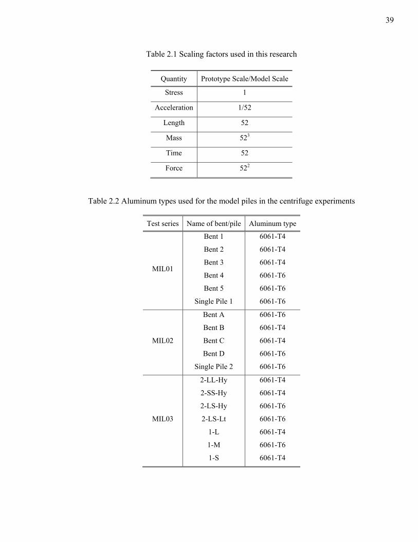
Table 2.1 Scaling factors used in this research
Quantity Prototype Scale/Model Scale
Stress 1
Acceleration 1/52
Length 52
Mass 523
Time 52
Force 522
Table 2.2 Aluminum types used for the model piles in the centrifuge experiments
Test series Name of bent/pile Aluminum type
MIL01
Bent 1
Bent 2
Bent 3
Bent 4
Bent 5
Single Pile 1
6061-T4
6061-T4
6061-T4
6061-T6
6061-T6
6061-T6
MIL02
Bent A
Bent B
Bent C
Bent D
Single Pile 2
6061-T6
6061-T4
6061-T4
6061-T6
6061-T6
MIL03
2-LL-Hy
2-SS-Hy
2-LS-Hy
2-LS-Lt
1-L
1-M
1-S
6061-T4
6061-T4
6061-T6
6061-T6
6061-T4
6061-T6
6061-T4
39
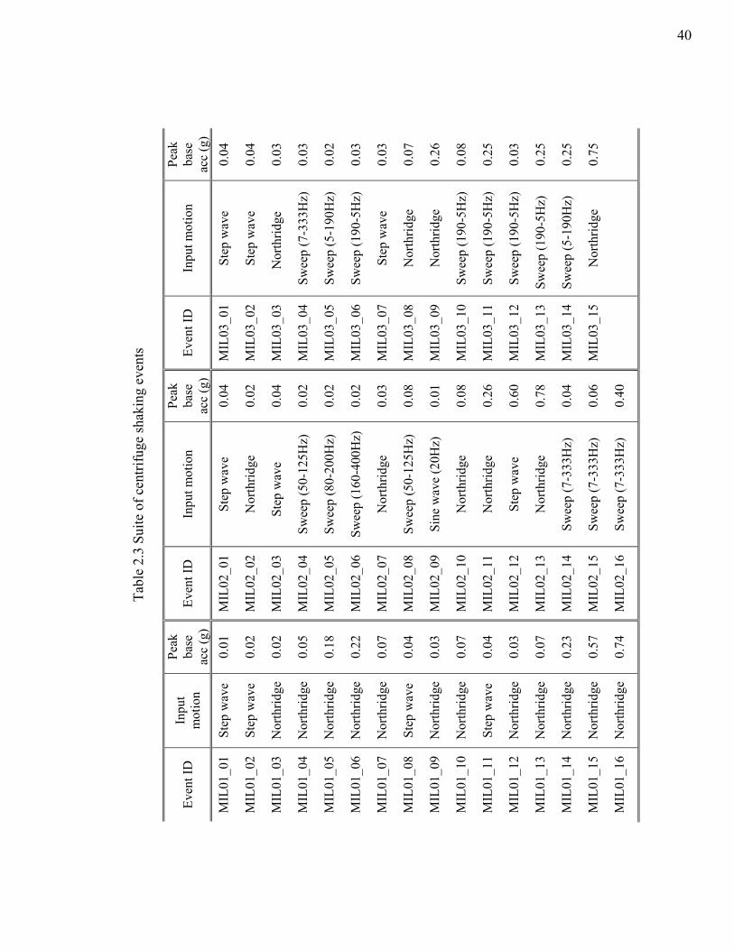
Tabl
e 2.
3 Su
ite o
f cen
trifu
ge sh
akin
g ev
ents
Even
t ID
In
put
mot
ion
Peak
ba
se
acc
(g)
Even
t ID
In
put m
otio
n Pe
ak
base
ac
c (g
) Ev
ent I
D
Inpu
t mot
ion
Peak
ba
se
acc
(g)
MIL
01_0
1
MIL
01_0
2
MIL
01_0
3
MIL
01_0
4
MIL
01_0
5
MIL
01_0
6
MIL
01_0
7
MIL
01_0
8
MIL
01_0
9
MIL
01_1
0
MIL
01_1
1
MIL
01_1
2
MIL
01_1
3
MIL
01_1
4
MIL
01_1
5
MIL
01_1
6
Step
wav
e
Step
wav
e
Nor
thrid
ge
Nor
thrid
ge
Nor
thrid
ge
Nor
thrid
ge
Nor
thrid
ge
Step
wav
e
Nor
thrid
ge
Nor
thrid
ge
Step
wav
e
Nor
thrid
ge
Nor
thrid
ge
Nor
thrid
ge
Nor
thrid
ge
Nor
thrid
ge
0.01
0.02
0.02
0.05
0.18
0.22
0.07
0.04
0.03
0.07
0.04
0.03
0.07
0.23
0.57
0.74
MIL
02_0
1
MIL
02_0
2
MIL
02_0
3
MIL
02_0
4
MIL
02_0
5
MIL
02_0
6
MIL
02_0
7
MIL
02_0
8
MIL
02_0
9
MIL
02_1
0
MIL
02_1
1
MIL
02_1
2
MIL
02_1
3
MIL
02_1
4
MIL
02_1
5
MIL
02_1
6
Step
wav
e
Nor
thrid
ge
Ste
p w
ave
Swee
p (5
0-12
5Hz)
Swee
p (8
0-20
0Hz)
Swee
p (1
60-4
00H
z)
Nor
thrid
ge
Swee
p (5
0-12
5Hz)
Sine
wav
e (2
0Hz)
Nor
thrid
ge
Nor
thrid
ge
Step
wav
e
Nor
thrid
ge
Swee
p (7
-333
Hz)
Swee
p (7
-333
Hz)
Swee
p (7
-333
Hz)
0.04
0.02
0.04
0.02
0.02
0.02
0.03
0.08
0.01
0.08
0.26
0.60
0.78
0.04
0.06
0.40
MIL
03_0
1
MIL
03_0
2
MIL
03_0
3
MIL
03_0
4
MIL
03_0
5
MIL
03_0
6
MIL
03_0
7
MIL
03_0
8
MIL
03_0
9
MIL
03_1
0
MIL
03_1
1
MIL
03_1
2
MIL
03_1
3
MIL
03_1
4
MIL
03_1
5
Step
wav
e
Step
wav
e
Nor
thrid
ge
Swee
p (7
-333
Hz)
Swee
p (5
-190
Hz)
Swee
p (1
90-5
Hz)
Step
wav
e
Nor
thrid
ge
Nor
thrid
ge
Swee
p (1
90-5
Hz)
Swee
p (1
90-5
Hz)
Swee
p (1
90-5
Hz)
Swee
p (1
90-5
Hz)
Swee
p (5
-190
Hz)
Nor
thrid
ge
0.04
0.04
0.03
0.03
0.02
0.03
0.03
0.07
0.26
0.08
0.25
0.03
0.25
0.25
0.75
40
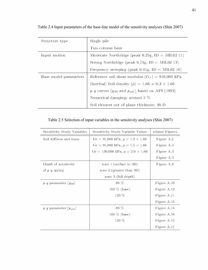
Table 2.4 Input parameters of the base-line model of the sensitivity analyses (Shin 2007)
Table 2.5 Selection of input variables in the sensitivity analyses (Shin 2007)
41
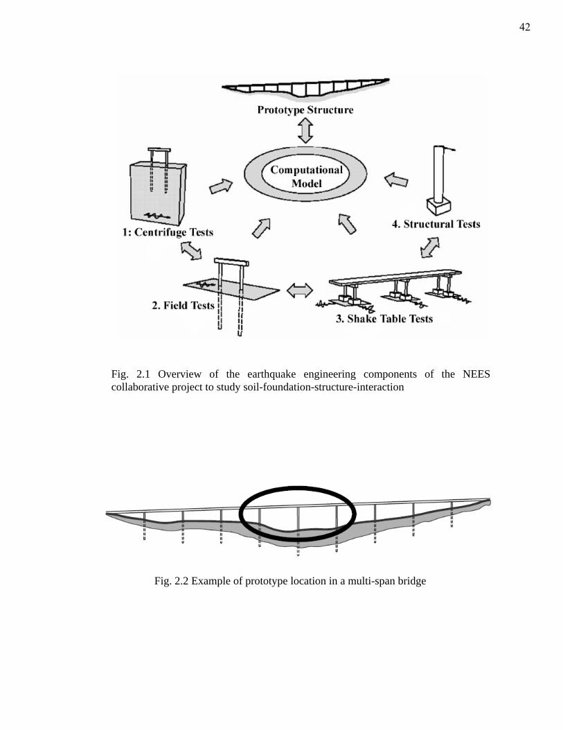
Fig. 2.2 Example of prototype location in a multi-span bridge
Fig. 2.1 Overview of the earthquake engineering components of the NEES collaborative project to study soil-foundation-structure-interaction
42
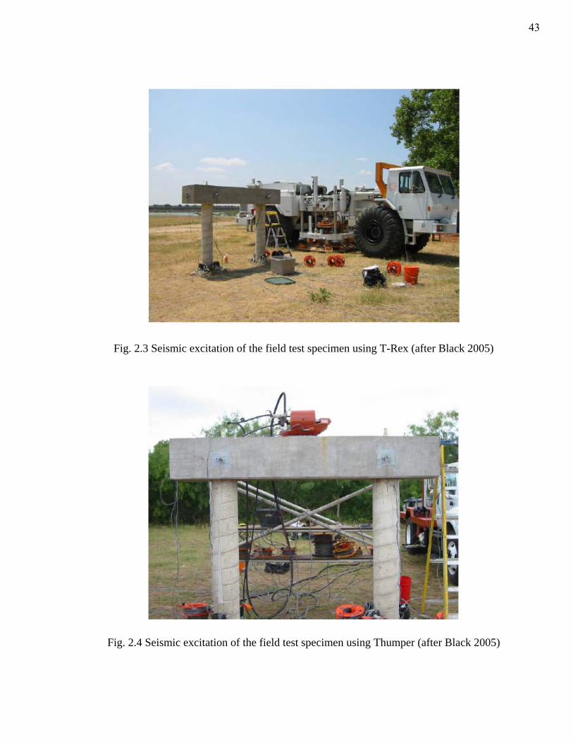
Fig. 2.3 Seismic excitation of the field test specimen using T-Rex (after Black 2005)
Fig. 2.4 Seismic excitation of the field test specimen using Thumper (after Black 2005)
43
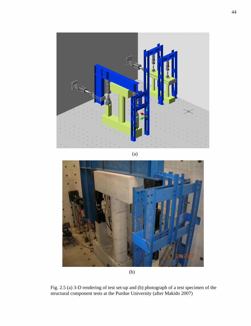
(a)
(a)
(b)
Fig. 2.5 (a) 3-D rendering of test set-up and (b) photograph of a test specimen of the structural component tests at the Purdue University (after Makido 2007)
44
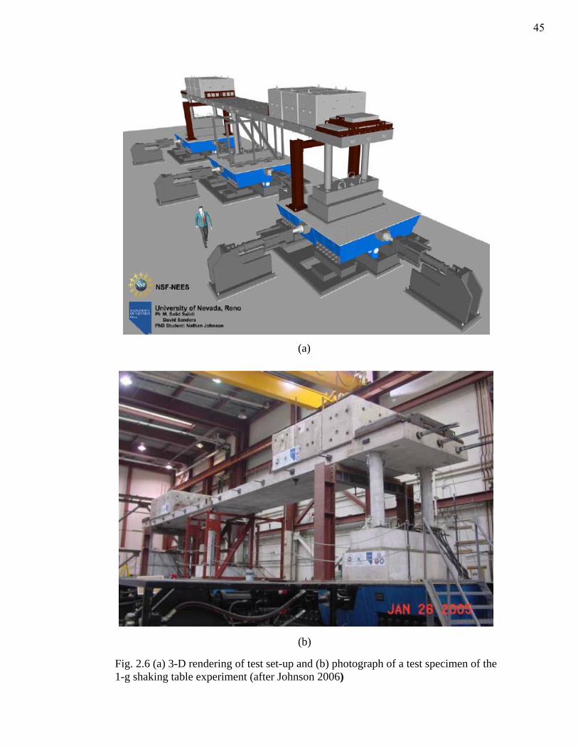
(a)
(b)
Fig. 2.6 (a) 3-D rendering of test set-up and (b) photograph of a test specimen of the 1-g shaking table experiment (after Johnson 2006)
45
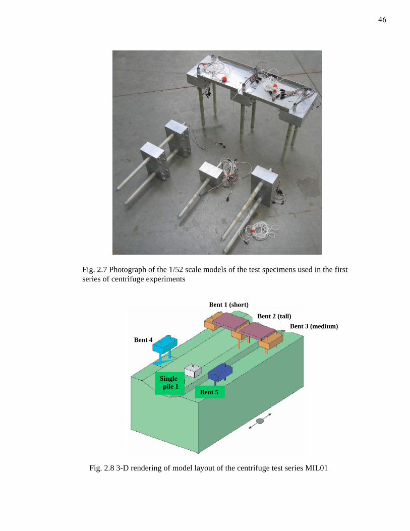
Fig. 2.7 Photograph of the 1/52 scale models of the test specimens used in the first series of centrifuge experiments
Bent 1 (short)
Bent 2 (tall) Bent 3 (medium)
Bent 5
Bent 4
Single pile 1
Fig. 2.8 3-D rendering of model layout of the centrifuge test series MIL01
46
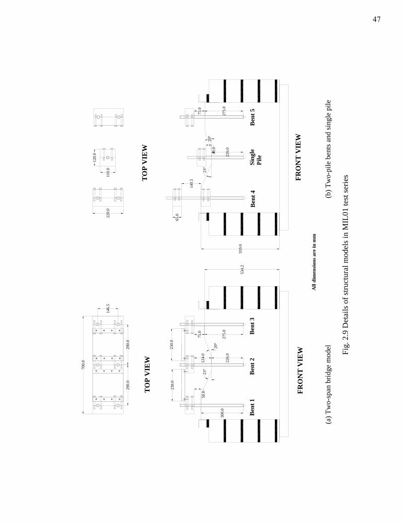
70
0.0
220.
011
0.0
120.
0
50.0
124.
075
.0
20°
23°
140.
5
20°
40.0
23°
75.0
230.
023
0.0
290.
029
0.0
146.
5
300.
0
65.0
TO
P V
IEW
TO
P V
IEW
FRO
NT
VIE
WFR
ON
T V
IEW
Ben
t 1B
ent 2
Ben
t 3B
ent 4
Sing
le
Pile
Ben
t 5
All
dim
ensi
ons a
re in
mm
226.
027
5.0
275.
022
6.0
534.
255
9.0
(a) T
wo-
span
brid
ge m
odel
(b
) Tw
o-pi
le b
ents
and
sing
le p
ile
Fig.
2.9
Det
ails
of s
truct
ural
mod
els i
n M
IL01
test
serie
s
47
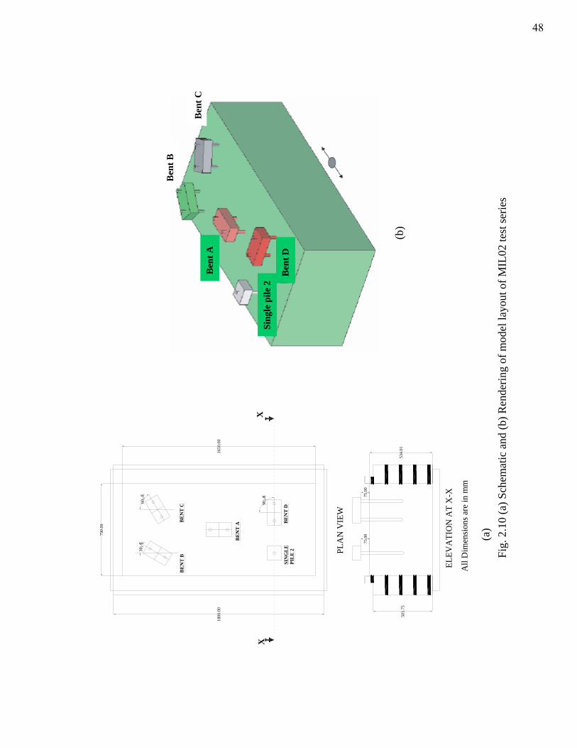
75.0
0
534.
01
75.0
0
All
Dim
ensi
ons a
re in
mm
BE
NT
D
BE
NT
BB
EN
T C
SIN
GL
EPI
LE
2
BE
NT
A
PLA
N V
IEW
XX
30¡Æ
60¡Æ
90¡Æ
ELEV
ATI
ON
AT
X-X
503.
75
1800
.00
790.
00
1650
.00
(a)
Ben
t B
Ben
t C
Ben
t A
Sing
le p
ile 2
Ben
t D
(b)
Fig.
2.1
0 (a
) Sch
emat
ic a
nd (b
) Ren
derin
g of
mod
el la
yout
of M
IL02
test
serie
s
48
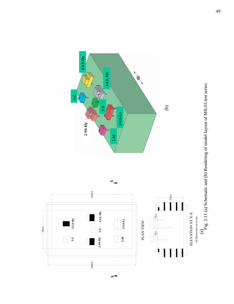
ELEV
ATI
ON
AT
X-X
PLA
N V
IEW
1-L
2-L
S-L
t
2-L
S-H
y
All
dim
ensi
ons a
re in
mm
1-S
2-SS
-Hy
534.
0
75.0
XX
2-L
L-H
y
1-M
75.0
1650
.0
790.
0
1800
.0
(a)
2-L
S-H
y
1-L
2-L
L-H
y
2-L
S-L
t
2-SS
-Hy
1-M
1-S (b)
Fig.
2.1
1 (a
) Sch
emat
ic a
nd (b
) Ren
derin
g of
mod
el la
yout
of M
IL03
test
serie
s
49
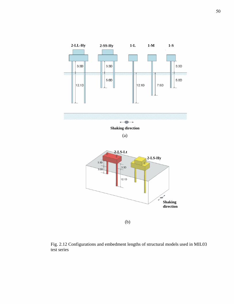
(a)
(b)
Shaking direction
Shaking direction
2-LL-Hy 2-SS-Hy 1-L 1-M 1-S
2-LS-Hy 2-LS-Lt
Fig. 2.12 Configurations and embedment lengths of structural models used in MIL03 test series
50
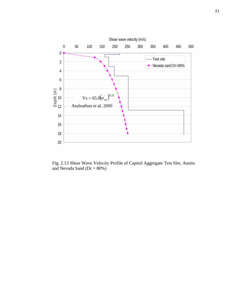
0
2
4
6
8
10
12
14
16
18
20
0 50 100 150 200 250 300 350 400 450 500
Shear wave velocity (m/s)
Dep
th (m
)Test siteNevada sand Dr=80%
Vs=65.8(σm') 0̂.25Arulnathan et al.(2000)( ) 25.0'
m8.65Vs σ=
Arulnathan et al. 2000
Fig. 2.13 Shear Wave Velocity Profile of Capitol Aggregate Test Site, Austin and Nevada Sand (Dr = 80%)
51
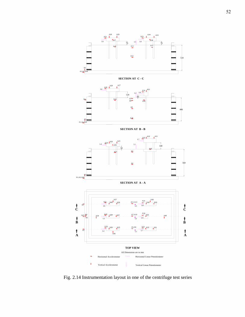
124
50
40
140
Horizontal Accelerometer
Vertical Accelerometer Vertical Linear Potentiometer
All Dimensions are in mm
TOP VIEW
Horizontal Linear Potentiometer
SECTION AT B - B
486
560
A A
SECTION AT A - A
1
A1
A20
A19
A21
A5,A6
A7-A10
A11,A12
A22
A24
A23
A26 A25
A28 A27
A30 A29 A34 A33
A35
A32 A31
A3A1,A2,A41
A2
A6
A5A13
A19A26 A25
A22A32 A31
A16
A36
A37 A38
L1 L7
L2 L9
L3 L8
A3
A4
A10
A9
A14A8A7
A18
L2A24 A35
L9
L6A20
A28 A27
L4
L5
L6
A3
A4
L7
L1L4 A36
A41 A39 A40
A1,A2,A41
BB
C C
L6
A1,A2,A41
A3
SECTION AT C - C
L3
A15 A11
A12
A29
76A37
A30A21
A17
A38L8
A23A34
76
A33
534
Fig. 2.14 Instrumentation layout in one of the centrifuge test series
52
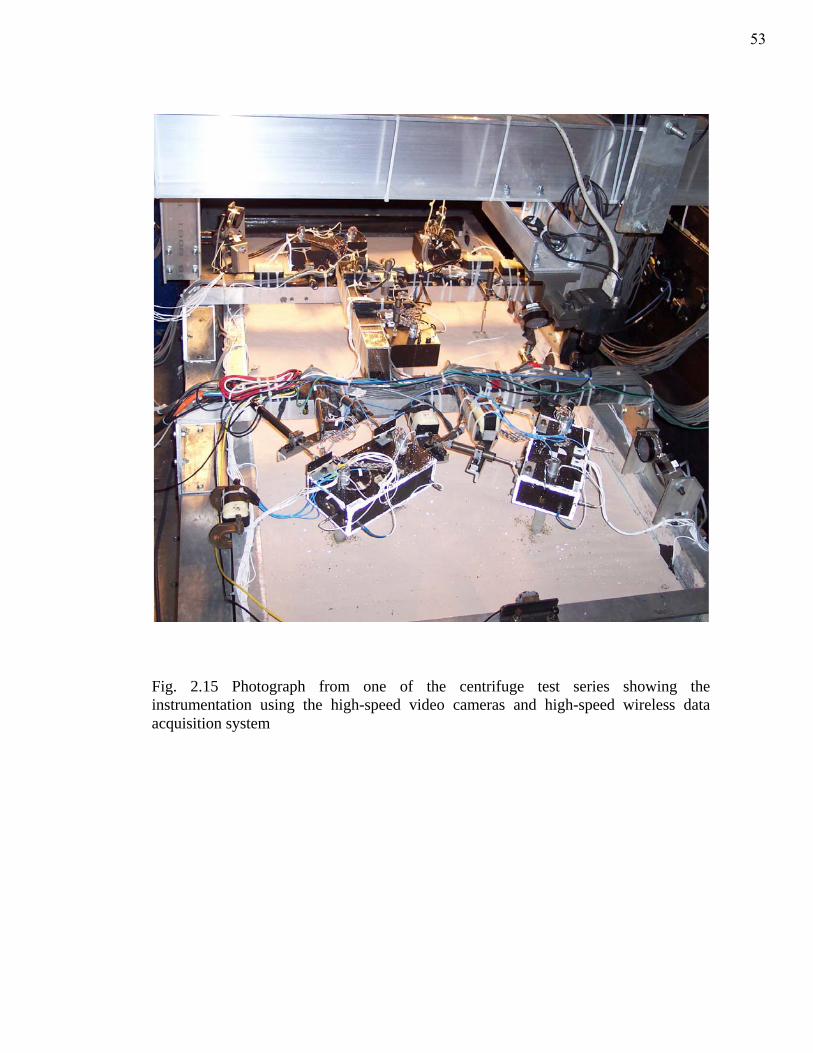
Fig. 2.15 Photograph from one of the centrifuge test series showing the instrumentation using the high-speed video cameras and high-speed wireless data acquisition system
53
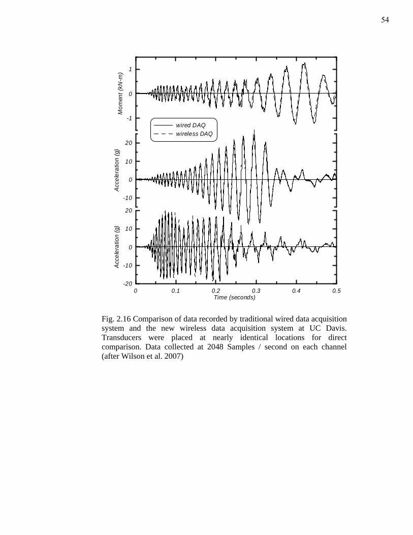
0 0.1 0.2 0.3 0.4 0.5Time (seconds)
-20
-10
0
10
20
Acc
eler
atio
n (g
)
-10
0
10
20
Acc
eler
atio
n (g
)-1
0
1
Mom
ent (
kN-m
)wired DAQwireless DAQ
Fig. 2.16 Comparison of data recorded by traditional wired data acquisition system and the new wireless data acquisition system at UC Davis. Transducers were placed at nearly identical locations for direct comparison. Data collected at 2048 Samples / second on each channel (after Wilson et al. 2007)
54
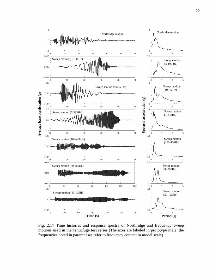
20 25 30 35 40 45 50-1
0
1
0 10 20 30 40 50-0.025
0.000
0.025
0 10 20 30 40 50-0.25
0.00
0.25
10 20 30 40 50 60 Spec
tral
acc
eler
atio
n (g
)
-0.5
0.0
0.5
10 20 30 40 50 60-0.05
0.00
0.05
0 20 40 60 80 100 120-0.05
0.00
0.05
Time (s)0 30 60 90 120 150 180
-0.05
0.00
0.05
0 1 2 30
3
0 1 2 30.0
0.2
0 1 2 30
2
0 1 2 30
4
0 1 2 30.0
0.2
0 1 2 30.0
0.2
0 1 2 30.0
0.2
Ave
rage
bas
e ac
cele
ratio
n (g
)
Period (s)
Northridge motionNorthridge motion
Sweep motion (5-190 Hz) Sweep motion (5-190 Hz)
Sweep motion (190-5 Hz) Sweep motion (190-5 Hz)
Sweep motion (7-333Hz) Sweep motion (7-333Hz)
Sweep motion (160-400Hz) Sweep motion (160-400Hz)
Sweep motion (80-200Hz) Sweep motion (80-200Hz)
Sweep motion (50-125Hz) Sweep motion (50-125Hz)
Fig. 2.17 Time histories and response spectra of Northridge and frequency sweep motions used in the centrifuge test series (The axes are labeled in prototype scale, the frequencies noted in parentheses refer to frequency content in model scale)
55
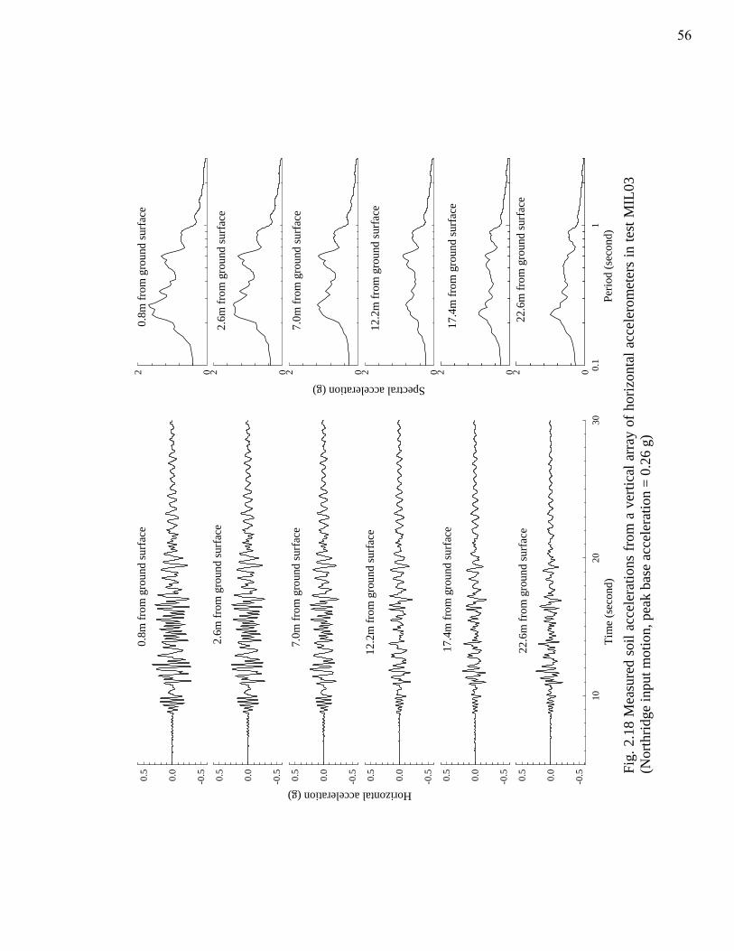
0.8m
from
gro
und
surf
ace
02
17.4
m fr
om g
roun
d su
rfac
e
Horizontal acceleration (g)
-0.50.0
0.5
22.6
m fr
om g
roun
d su
rfac
e
Tim
e (s
econ
d)10
2030
-0.50.0
0.5
12.2
m fr
om g
roun
d su
rfac
e
-0.50.0
0.5
12.2
m fr
om g
roun
d su
rfac
e
02
22.6
m fr
om g
roun
d su
rfac
e
Perio
d (s
econ
d)0.
11
02
17.4
m fr
om g
roun
d su
rfac
e
Spectral acceleration (g)
02
7.0m
from
gro
und
surf
ace
-0.50.0
0.5
7.0m
from
gro
und
surf
ace
02
2.6m
from
gro
und
surf
ace
-0.50.0
0.5
0.8m
from
gro
und
surf
ace
-0.50.0
0.5
022.
6m fr
om g
roun
d su
rfac
e
Fig.
2.1
8 M
easu
red
soil
acce
lera
tions
from
a v
ertic
al a
rray
of h
oriz
onta
l acc
eler
omet
ers
in te
st M
IL03
(N
orth
ridge
inpu
t mot
ion,
pea
k ba
se a
ccel
erat
ion
= 0.
26 g
)
56
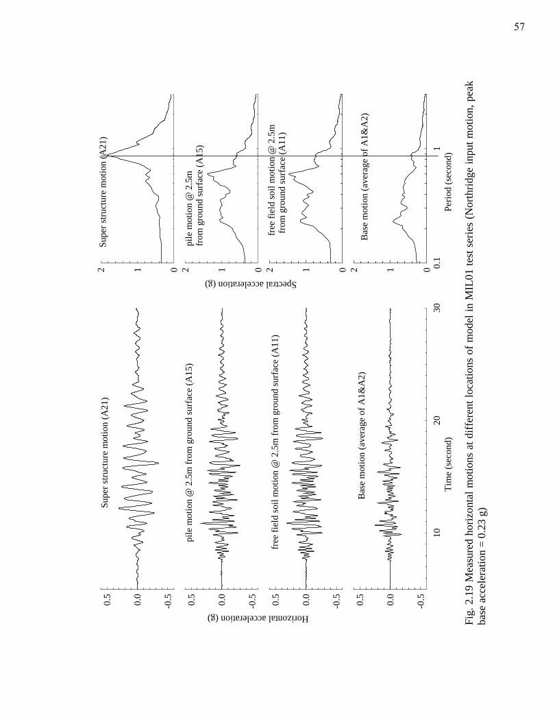
Fig.
2.1
9 M
easu
red
horiz
onta
l mot
ions
at d
iffer
ent l
ocat
ions
of m
odel
in M
IL01
test
ser
ies
(Nor
thrid
ge in
put m
otio
n, p
eak
base
acc
eler
atio
n =
0.23
g)
free
fiel
d so
il m
otio
n @
2.5
m fr
om g
roun
d su
rfac
e (A
11)
Horizontal acceleration (g)
-0.50.0
0.5
Bas
e m
otio
n (a
vera
ge o
f A1&
A2)
Tim
e (s
econ
d)10
2030
-0.50.0
0.5
pile
mot
ion
@ 2
.5m
from
gro
und
surf
ace
(A15
)
-0.50.0
0.5
pile
mot
ion
@ 2
.5m
fr
om g
roun
d su
rfac
e (A
15)
012
Bas
e m
otio
n (a
vera
ge o
f A1&
A2)
Perio
d (s
econ
d)0.
11
012
free
fiel
d so
il m
otio
n @
2.5
m fr
om g
roun
d su
rfac
e (A
11)
Spectral acceleration (g)
012
Supe
r stru
ctur
e m
otio
n (A
21)
-0.50.0
0.5
Supe
r stru
ctur
e m
otio
n (A
21)
012
57
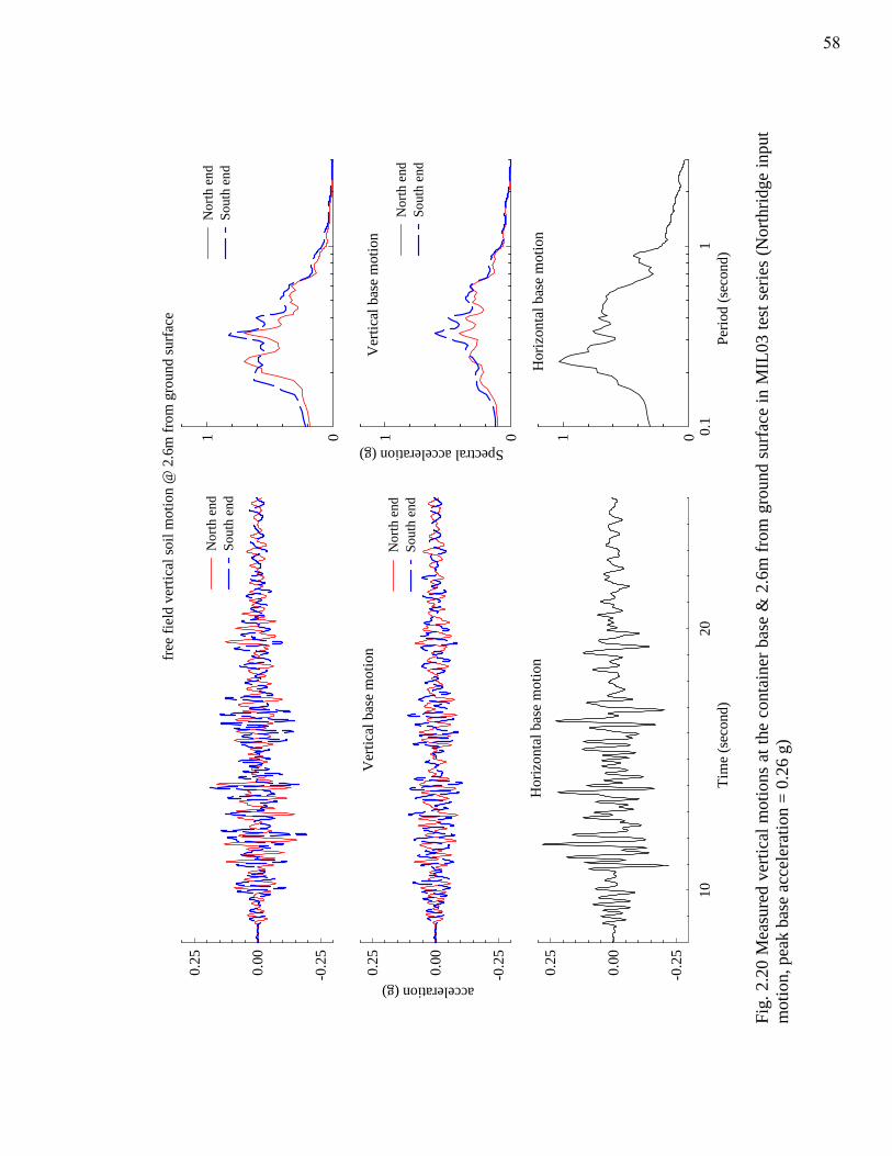
Ver
tical
bas
e m
otio
n
acceleration (g) -0.2
5
0.00
0.25
Nor
th e
ndSo
uth
end
Hor
izon
tal b
ase
mot
ion
Tim
e (s
econ
d)10
20
-0.2
5
0.00
0.25
Perio
d (s
econ
d)0.
11
01
Ver
tical
bas
e m
otio
n
Spectral acceleration (g) 01
free
fiel
d ve
rtica
l soi
l mot
ion
@ 2
.6m
from
gro
und
surf
ace
-0.2
5
0.00
0.25
01
Hor
izon
tal b
ase
mot
ion
Nor
th e
ndSo
uth
end
Nor
th e
ndSo
uth
end
Nor
th e
ndSo
uth
end
Fig.
2.2
0 M
easu
red
verti
cal m
otio
ns a
t the
con
tain
er b
ase
& 2
.6m
from
gro
und
surf
ace
in M
IL03
test
ser
ies
(Nor
thrid
ge in
put
mot
ion,
pea
k ba
se a
ccel
erat
ion
= 0.
26 g
)
58
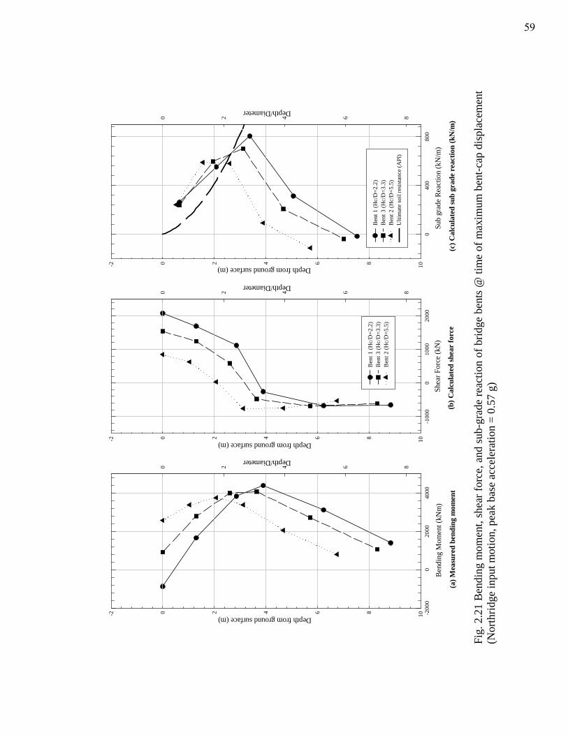
(a) M
easu
red
bend
ing
mom
ent
Ben
ding
Mom
ent (
kNm
)-2
000
020
0040
00
Depth/Diameter
0 2 4 6 8
Depth from ground surface (m)-2 0 2 4 6 8 10
(b) C
alcu
late
d sh
ear
forc
e
Shea
r For
ce (k
N)
-100
00
1000
2000
Depth/Diameter
0 2 4 6 8
Depth from ground surface (m)-2 0 2 4 6 8 10
(c) C
alcu
late
d su
b gr
ade
reac
tion
(kN
/m)
Sub
grad
e R
eact
ion
(kN
/m)
040
080
0
Depth/Diameter
0 2 4 6 8
Depth from ground surface (m)-2 0 2 4 6 8 10
Ben
t 1 (H
c/D
=2.2
)B
ent 3
(Hc/
D=3
.3)
Ben
t 2 (H
c/D
=5.5
)U
ltim
ate
soil
resi
stan
ce (A
PI)
Ben
t 1 (H
c/D
=2.2
)B
ent 3
(Hc/
D=3
.3)
Ben
t 2 (H
c/D
=5.5
)
Fig.
2.2
1 B
endi
ng m
omen
t, sh
ear f
orce
, and
sub
-gra
de re
actio
n of
brid
ge b
ents
@ ti
me
of m
axim
um b
ent-c
ap d
ispl
acem
ent
(Nor
thrid
ge in
put m
otio
n, p
eak
base
acc
eler
atio
n =
0.57
g)
59
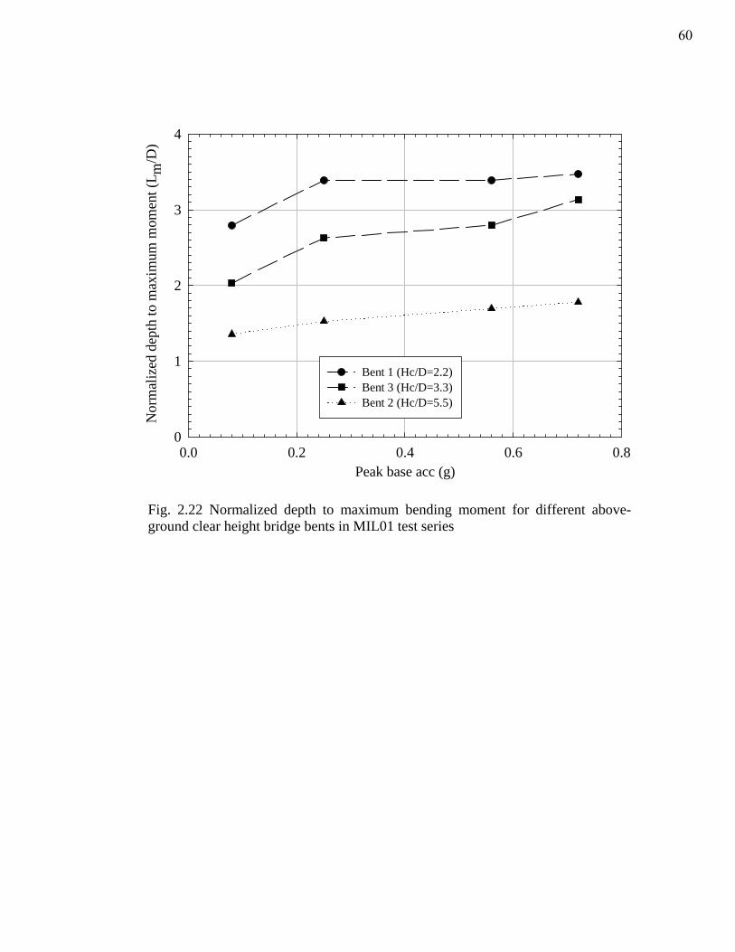
Peak base acc (g)0.0 0.2 0.4 0.6 0.8
Nor
mal
ized
dep
th to
max
imum
mom
ent (
L m/D
)
0
1
2
3
4
Bent 1 (Hc/D=2.2)Bent 3 (Hc/D=3.3)Bent 2 (Hc/D=5.5)
Fig. 2.22 Normalized depth to maximum bending moment for different above-ground clear height bridge bents in MIL01 test series
60
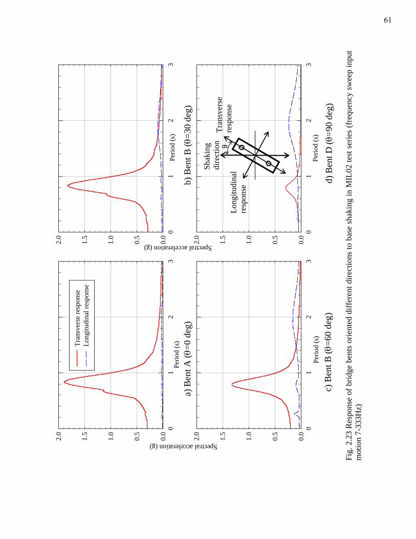
a) B
ent A
(θ=0
deg
)
01
23
Spectral acceleration (g) 0.0
0.5
1.0
1.5
2.0
Tran
sver
se re
spon
seLo
ngitu
dina
l res
pons
e
Perio
d (s
)
01
23
0.0
0.5
1.0
1.5
2.0
01
23
0.0
0.5
1.0
1.5
2.0
01
23
0.0
0.5
1.0
1.5
2.0
Perio
d (s
)
b) B
ent B
(θ=3
0 de
g)
c) B
ent B
(θ=6
0 de
g)d)
Ben
t D (θ
=90
deg)
Perio
d (s
)Pe
riod
(s)
Spectral acceleration (g)
Long
itudi
nal
resp
onse
Shak
ing
dire
ctio
n Tr
ansv
erse
re
spon
se
θ
Fig.
2.2
3 R
espo
nse
of b
ridge
ben
ts o
rient
ed d
iffer
ent d
irect
ions
to b
ase
shak
ing
in M
IL02
test
ser
ies
(fre
quen
cy s
wee
p in
put
mot
ion
7-33
3Hz)
61
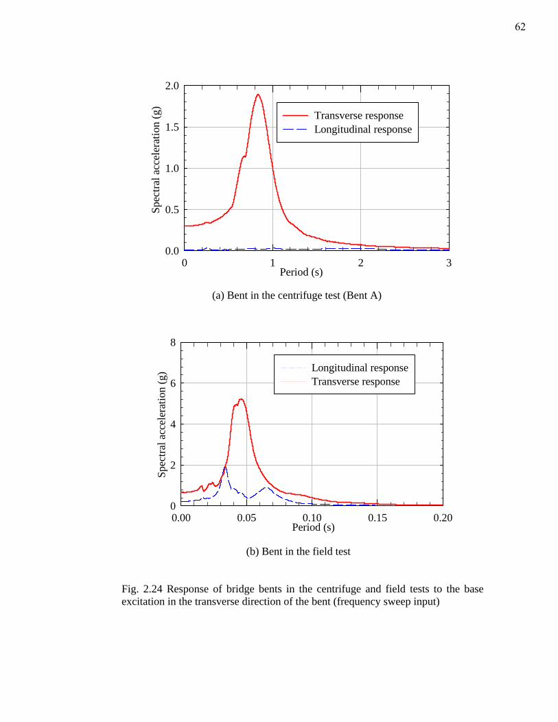
Fig. 2.24 Response of bridge bents in the centrifuge and field tests to the base excitation in the transverse direction of the bent (frequency sweep input)
0.00 0.05 0.10 0.15 0.20
Spec
tral a
ccel
erat
ion
(g)
0
2
4
6
8
Longitudinal responseTransverse response
Period (s)
(b) Bent in the field test
Period (s)0 1 2 3
Spec
tral a
ccel
erat
ion
(g)
0.0
0.5
1.0
1.5
2.0
Transverse responseLongitudinal response
(a) Bent in the centrifuge test (Bent A)
62
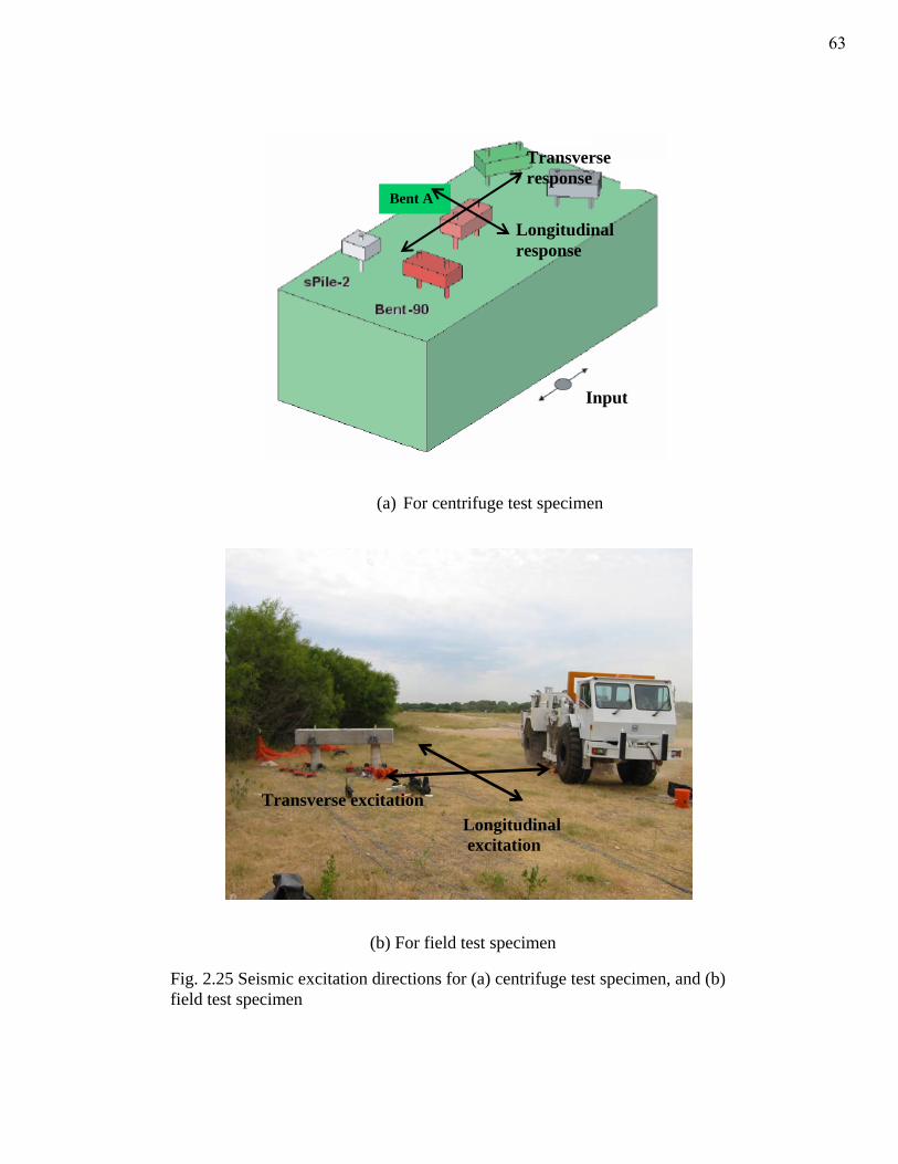
Fig. 2.25 Seismic excitation directions for (a) centrifuge test specimen, and (b) field test specimen
(a) For centrifuge test specimen
Bent A
Transverse response
Longitudinal response
Input
(b) For field test specimen
Transverse excitation Longitudinal excitation
63
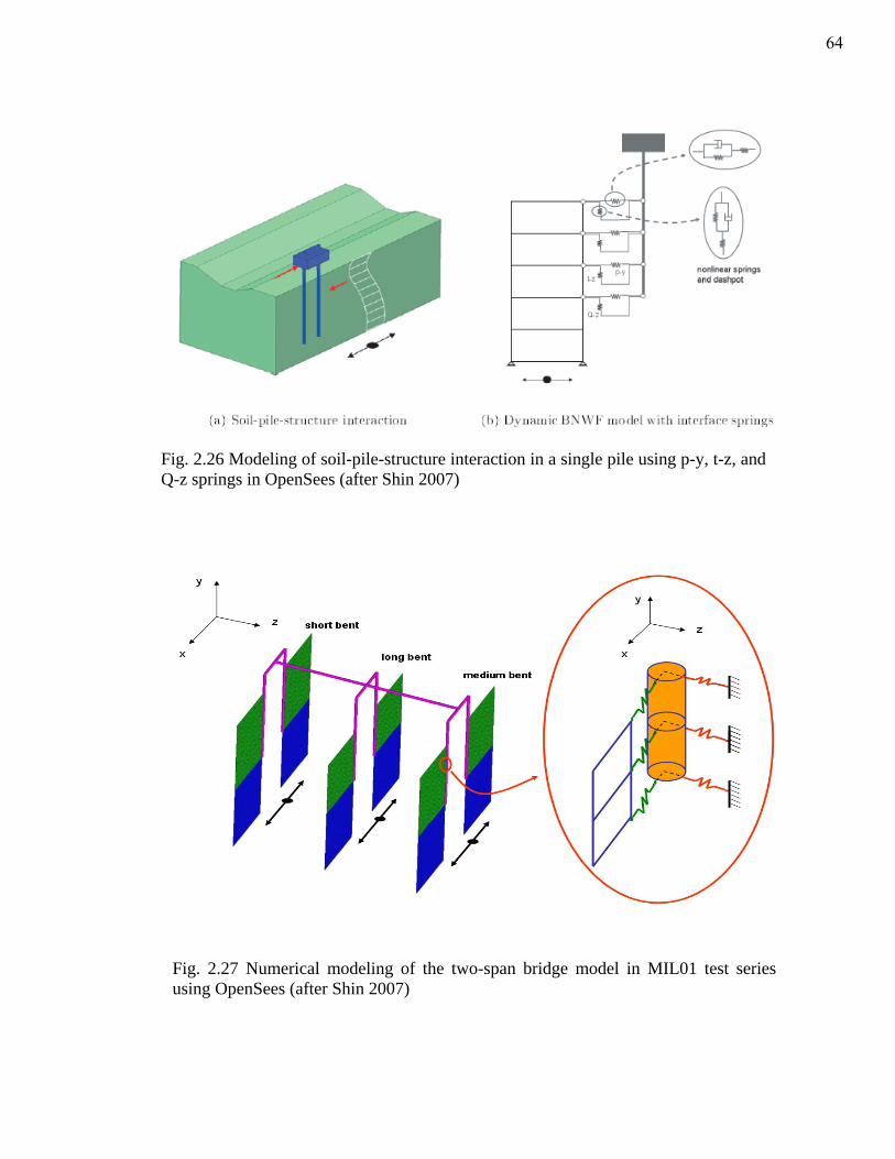
Fig. 2.26 Modeling of soil-pile-structure interaction in a single pile using p-y, t-z, and Q-z springs in OpenSees (after Shin 2007)
Fig. 2.27 Numerical modeling of the two-span bridge model in MIL01 test series using OpenSees (after Shin 2007)
64
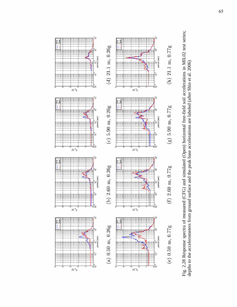
Fig.
2.2
8 R
espo
nse
spec
tra o
f mea
sure
d (C
FG) a
nd s
imul
ated
(Ope
n) h
oriz
onta
l fre
e-fie
ld s
oil a
ccel
erat
ions
in M
IL02
test
ser
ies;
de
pths
to th
e ac
cele
rom
eter
s fro
m g
roun
d su
rfac
e an
d th
e pe
ak b
ase
acce
lera
tions
are
labe
led
(afte
r Shi
n et
al.
2006
)
65
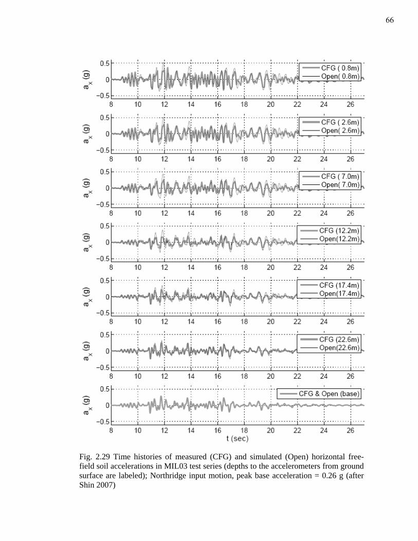
Fig. 2.29 Time histories of measured (CFG) and simulated (Open) horizontal free-field soil accelerations in MIL03 test series (depths to the accelerometers from ground surface are labeled); Northridge input motion, peak base acceleration = 0.26 g (after Shin 2007)
66
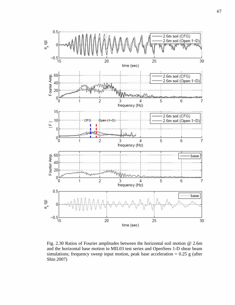
Fig. 2.30 Ratios of Fourier amplitudes between the horizontal soil motion @ 2.6m and the horizontal base motion in MIL03 test series and OpenSees 1-D shear beam simulations; frequency sweep input motion, peak base acceleration = 0.25 g (after Shin 2007)
67
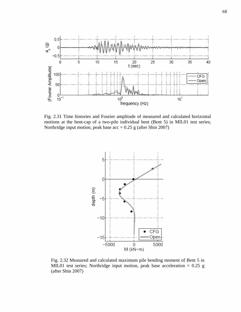
Fig. 2.31 Time histories and Fourier amplitude of measured and calculated horizontal motions at the bent-cap of a two-pile individual bent (Bent 5) in MIL01 test series; Northridge input motion, peak base acc = 0.25 g (after Shin 2007)
Fig. 2.32 Measured and calculated maximum pile bending moment of Bent 5 in MIL01 test series; Northridge input motion, peak base acceleration = 0.25 g (after Shin 2007)
68
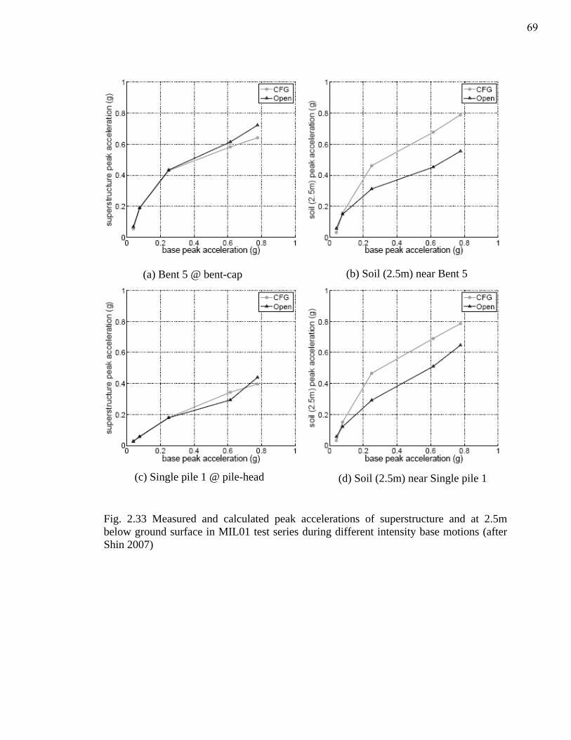
(a) Bent 5 @ bent-cap (b) Soil (2.5m) near Bent 5
(c) Single pile 1 @ pile-head (d) Soil (2.5m) near Single pile 1
Fig. 2.33 Measured and calculated peak accelerations of superstructure and at 2.5m below ground surface in MIL01 test series during different intensity base motions (after Shin 2007)
69
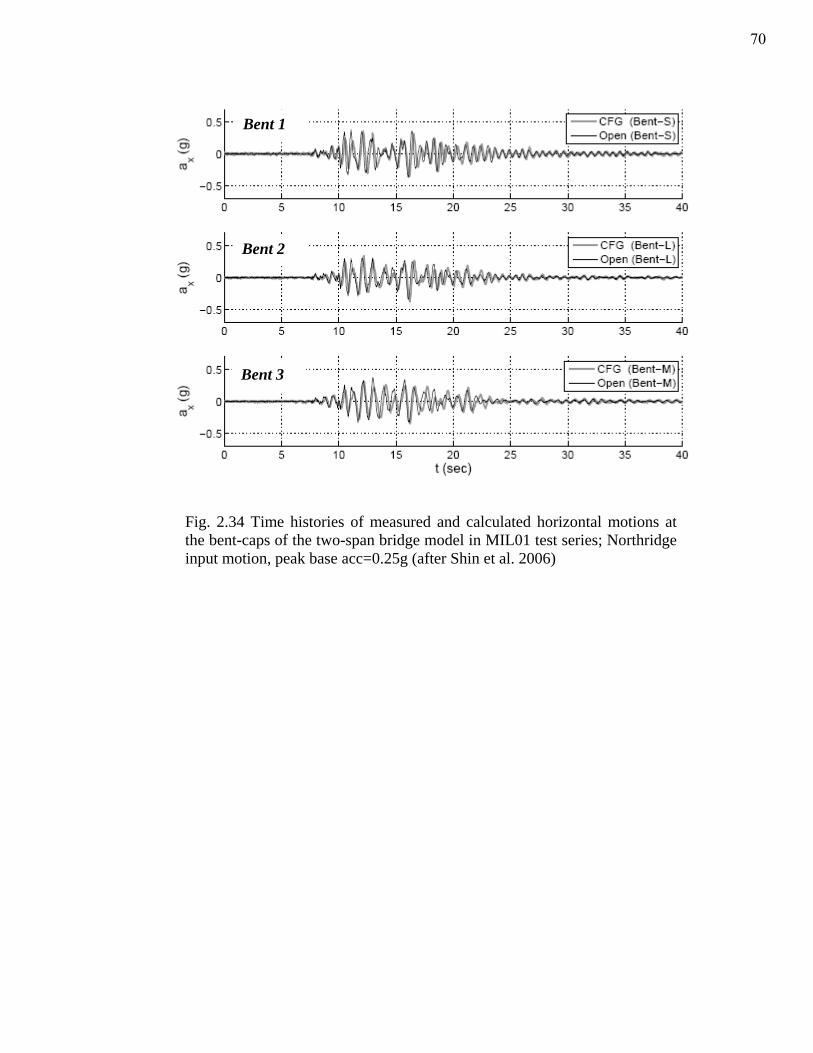
Bent 1
Bent 2
Bent 3
Fig. 2.34 Time histories of measured and calculated horizontal motions at the bent-caps of the two-span bridge model in MIL01 test series; Northridge input motion, peak base acc=0.25g (after Shin et al. 2006)
70
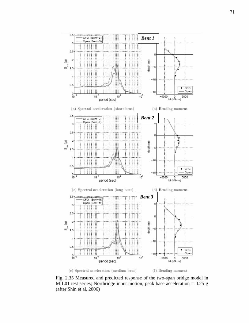
Bent 1
Bent 2
Bent 3
Fig. 2.35 Measured and predicted response of the two-span bridge model in MIL01 test series; Northridge input motion, peak base acceleration = 0.25 g (after Shin et al. 2006)
71
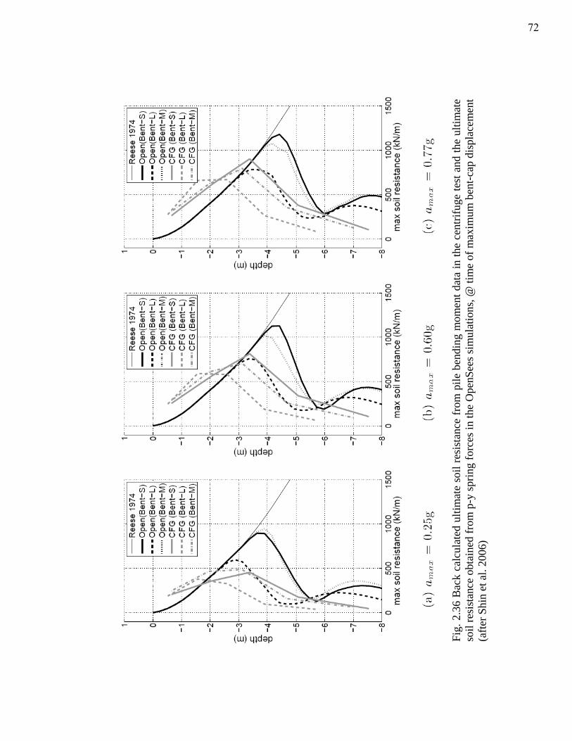
Fig.
2.3
6 B
ack
calc
ulat
ed u
ltim
ate
soil
resi
stan
ce fr
om p
ile b
endi
ng m
omen
t dat
a in
the
cent
rifug
e te
st a
nd th
e ul
timat
e so
il re
sist
ance
obt
aine
d fr
om p
-y sp
ring
forc
es in
the
Ope
nSee
s sim
ulat
ions
, @ ti
me
of m
axim
um b
ent-c
ap d
ispl
acem
ent
(afte
r Shi
n et
al.
2006
)
72
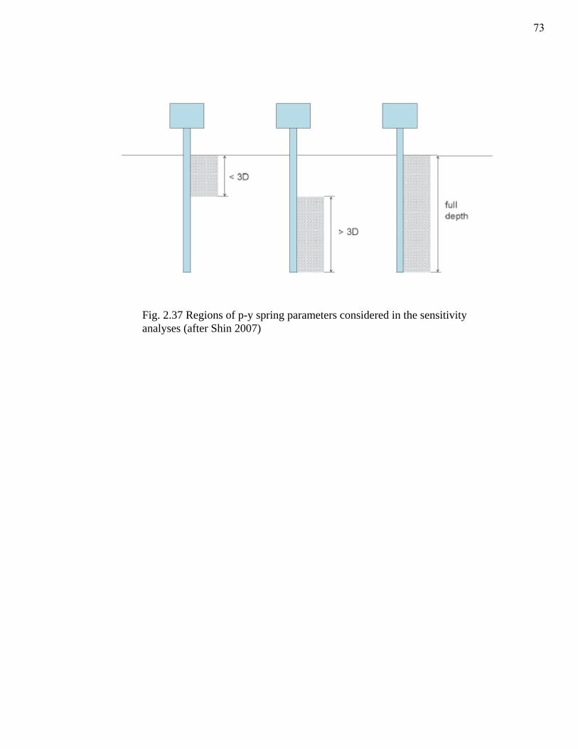
Fig. 2.37 Regions of p-y spring parameters considered in the sensitivity analyses (after Shin 2007)
73
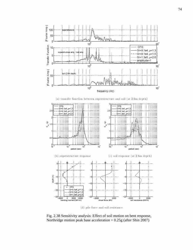
Fig. 2.38 Sensitivity analysis: Effect of soil motion on bent response, Northridge motion peak base acceleration = 0.25g (after Shin 2007)
74
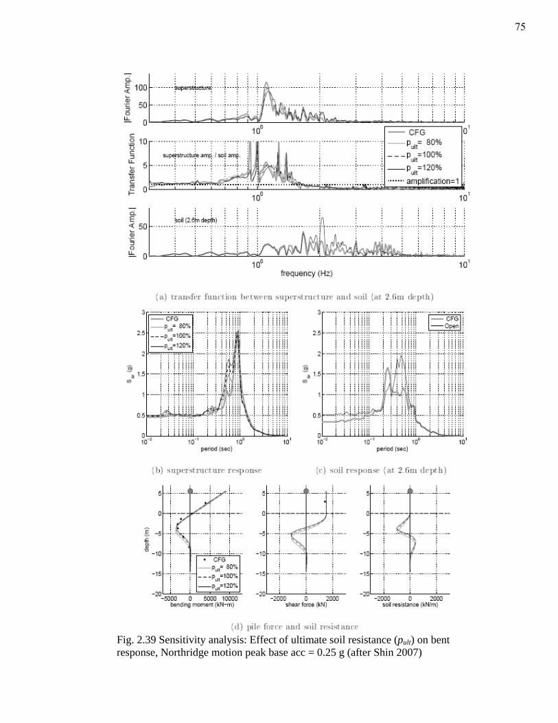
Fig. 2.39 Sensitivity analysis: Effect of ultimate soil resistance (pult) on bent
response, Northridge motion peak base acc = 0.25 g (after Shin 2007)
75
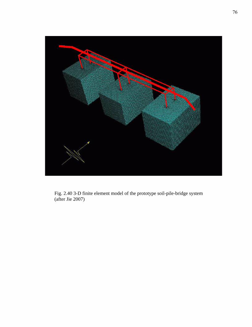
Fig. 2.40 3-D finite element model of the prototype soil-pile-bridge system (after Jie 2007)
76
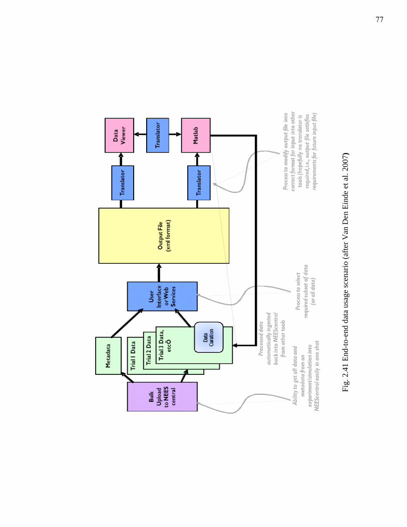
Fig.
2.4
1 En
d-to
-end
dat
a us
age
scen
ario
(afte
r Van
Den
Ein
de e
t al.
2007
)
77
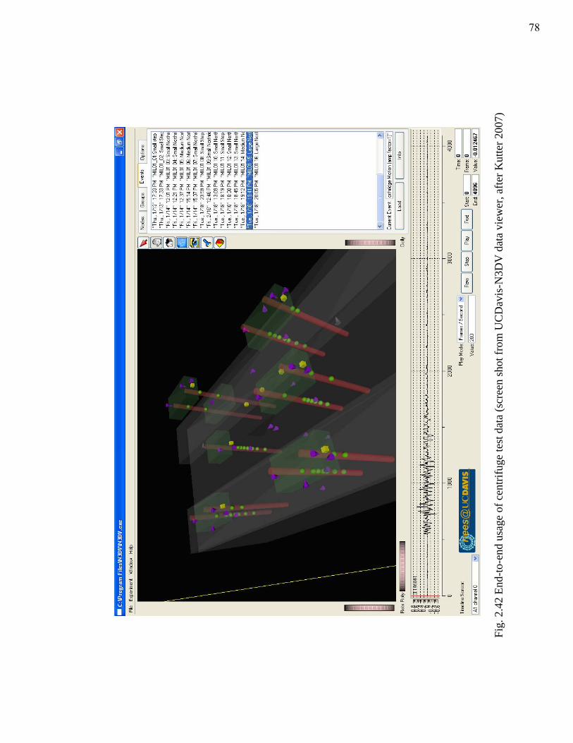
Fig.
2.4
2 En
d-to
-end
usa
ge o
f cen
trifu
ge te
st d
ata
(scr
een
shot
from
UC
Dav
is-N
3DV
dat
a vi
ewer
, afte
r Kut
ter 2
007)
78
Chapter 3
Comparison of centrifuge and 1g shake table models of a pile supported
bridge structure
This chapter presents the comparison of experimental results and the resolution of
issues associated with comparing physical models of a, two-span, pile supported bridge
structure tested at different experimental facilities, at different scale, using different test
boundary conditions, and scaling laws. A comparison between the system response of
bridge model and component response of individual bents during a series of shaking
events also presented in this chapter. The contents of this chapter are adapted from two
published papers. The complete references of these papers and the contribution of
different authors are given below
1. Ilankatharan, M., Kutter, B.L., H. Shin, P. Arduino, S.L. Kramer, N. Johnson, and T.
Sasaki. (2006). “Comparison of Centrifuge and 1g Shaking Table Models of a Pile
Supported Bridge Structure,” Proceedings of the 6th International Conference on
Physical Modeling in Geotechnics, Hong Kong, Vol. 2: 1313-1318, August, 2006.
2. Kutter, B.L., and Wilson, D.W. (2006). "Physical Modeling of Dynamic Behavior of
Soil-Foundation-Superstructure Systems," Invited paper, International Journal of
Physical Modelling in Geotechnics. Vol. 6 No. 1, pp. 1-12.
H. Shin assisted with the centrifuge experiment and performed numerical
simulations of the experiments, T. Sasaki assisted with the centrifuge experiment, N.
Johnson provided 1-g shake table experiment data, and P. Ardunio and S. L. Kramer
79
provided valuable advice in the course of the study. The centrifuge testing of the two-
span section of the bridge model described in Chapter 2 of this dissertation, including the
collaborative test design process and some representative results were presented in the
second paper. The figures in the paper corresponding to above study were created by the
author of this dissertation.
Abstract: In small-scale centrifuge tests, it is difficult to accurately model reinforced
concrete structures; in large-scale 1-g shake table tests it is difficult to accurately model
geotechnical aspects of soil-pile-structure interaction. To provide a comprehensive
validation of a numerical procedure for analyzing the behavior of a bridge supported on
piles, a series of experiments has been conducted using centrifuge and shake tables. Two
seemingly basic questions that were difficult for the interdisciplinary research team to
resolve were: What clear height (between ground surface and bridge deck) should be
used in the centrifuge model to correspond to the fixed-fixed boundary conditions for the
pile extensions in the shake table tests, and what input motions should be used in the
shake table test to most closely correspond to the centrifuge tests? To resolve these
questions, an equivalent depth to fixity of the piles in the centrifuge were calculated, and
the free-field ground motion close to anticipated fixity point was used as a command
input motion for the 1-g shake table test. These assumptions enabled observation of
reasonable comparisons between bridge deck responses in both experiments. This
chapter presents these comparisons and discusses the above questions and other aspects
of the design of the centrifuge models. Further, this chapter compares the system
response of the centrifuge bridge model with that of component response during a series
of earthquake simulations.
80
3.1 Introduction
Past earthquakes, particularly the 1989 Loma Prieta and 1994 Northridge
earthquakes in California, and the 1995 Kobe earthquake in Japan, have caused collapse
of, or severe damage to, a considerable number of major bridges that were designed for
seismic forces (Priestly et al. 1998). One major reason for the poor performance relates to
the complexities of the bridge structural and sub structural systems as compared to other
structures. The ground motion and the nonlinear characteristics of the soil, foundation,
and structure influence the dynamic response of a bridge structure. For most bridges, the
foundation system may be designed to remain elastic while the pier portion of the
substructure is detailed for inelastic deformations and energy dissipation. This approach
is intended to avoid the difficulty of post earthquake inspection and the high cost
associated with repair of damaged foundation (Chai, 2002). This approach often leads to
very expensive design for new construction or seismic retrofits of bridges. Dissipation of
energy by the yielding of soil and foundations they support can influence the structural
performance (Gazetas et al, 1998). The degree and nature of these effects, however, are
not well defined by documented field evidence or by experimental testing. The accurate
evaluation of the seismic response of a bridge is limited by the ability to model the
behavior and interaction between a structure, its foundation and the supporting soil. It is,
however, impractical to test a single physical model of the prototype SFSI system at
reasonable scale and reproduce all key aspects of the system performance. Therefore, a
series of four complementary experimental programs had been conducted using the
NEES field shakers at the University of Texas, Austin, the large scale structural testing
facility at the Purdue University, the large scale shake tables at the University of Nevada,
81
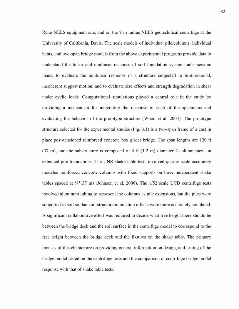
Reno NEES equipment site, and on the 9 m radius NEES geotechnical centrifuge at the
University of California, Davis. The scale models of individual pile/columns, individual
bents, and two-span bridge models from the above experimental programs provide data to
understand the linear and nonlinear response of soil foundation system under seismic
loads, to evaluate the nonlinear response of a structure subjected to bi-directional,
incoherent support motion, and to evaluate size effects and strength degradation in shear
under cyclic loads. Computational simulations played a central role in the study by
providing a mechanism for integrating the response of each of the specimens and
evaluating the behavior of the prototype structure (Wood et al, 2004). The prototype
structure selected for the experimental studies (Fig. 3.1) is a two-span frame of a cast in
place post-tensioned reinforced concrete box girder bridge. The span lengths are 120 ft
(37 m), and the substructure is composed of 4 ft (1.2 m) diameter 2-column piers on
extended pile foundations. The UNR shake table tests involved quarter scale accurately
modeled reinforced concrete columns with fixed supports on three independent shake
tables spaced at ¼*(37 m) (Johnson et al, 2006). The 1/52 scale UCD centrifuge tests
involved aluminum tubing to represent the columns as pile extensions, but the piles were
supported in soil so that soil-structure interaction effects were more accurately simulated.
A significant collaborative effort was required to decide what free height there should be
between the bridge deck and the soil surface in the centrifuge model to correspond to the
free height between the bridge deck and the fixtures on the shake table. The primary
focuses of this chapter are on providing general information on design, and testing of the
bridge model tested on the centrifuge tests and the comparison of centrifuge bridge model
response with that of shake table tests.
82
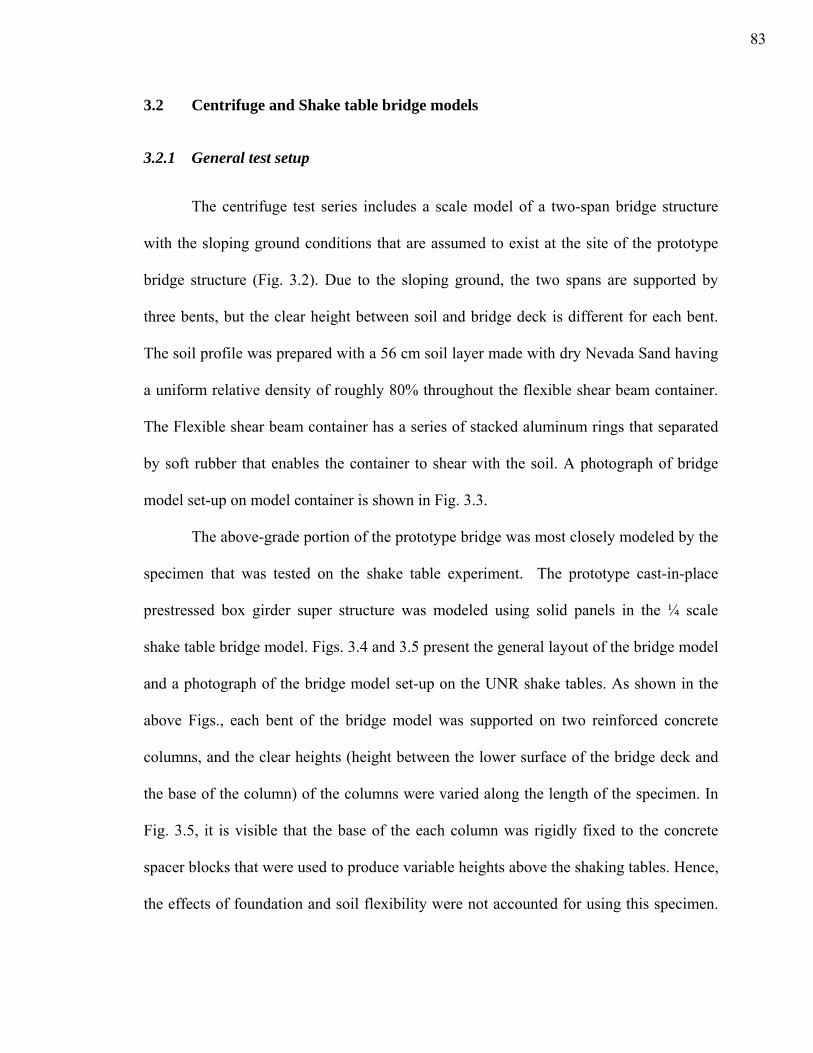
3.2 Centrifuge and Shake table bridge models
3.2.1 General test setup
The centrifuge test series includes a scale model of a two-span bridge structure
with the sloping ground conditions that are assumed to exist at the site of the prototype
bridge structure (Fig. 3.2). Due to the sloping ground, the two spans are supported by
three bents, but the clear height between soil and bridge deck is different for each bent.
The soil profile was prepared with a 56 cm soil layer made with dry Nevada Sand having
a uniform relative density of roughly 80% throughout the flexible shear beam container.
The Flexible shear beam container has a series of stacked aluminum rings that separated
by soft rubber that enables the container to shear with the soil. A photograph of bridge
model set-up on model container is shown in Fig. 3.3.
The above-grade portion of the prototype bridge was most closely modeled by the
specimen that was tested on the shake table experiment. The prototype cast-in-place
prestressed box girder super structure was modeled using solid panels in the ¼ scale
shake table bridge model. Figs. 3.4 and 3.5 present the general layout of the bridge model
and a photograph of the bridge model set-up on the UNR shake tables. As shown in the
above Figs., each bent of the bridge model was supported on two reinforced concrete
columns, and the clear heights (height between the lower surface of the bridge deck and
the base of the column) of the columns were varied along the length of the specimen. In
Fig. 3.5, it is visible that the base of the each column was rigidly fixed to the concrete
spacer blocks that were used to produce variable heights above the shaking tables. Hence,
the effects of foundation and soil flexibility were not accounted for using this specimen.
83
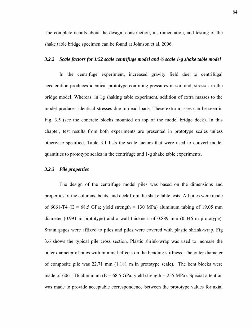
The complete details about the design, construction, instrumentation, and testing of the
shake table bridge specimen can be found at Johnson et al. 2006.
3.2.2 Scale factors for 1/52 scale centrifuge model and ¼ scale 1-g shake table model
In the centrifuge experiment, increased gravity field due to centrifugal
acceleration produces identical prototype confining pressures in soil and, stresses in the
bridge model. Whereas, in 1g shaking table experiment, addition of extra masses to the
model produces identical stresses due to dead loads. These extra masses can be seen in
Fig. 3.5 (see the concrete blocks mounted on top of the model bridge deck). In this
chapter, test results from both experiments are presented in prototype scales unless
otherwise specified. Table 3.1 lists the scale factors that were used to convert model
quantities to prototype scales in the centrifuge and 1-g shake table experiments.
3.2.3 Pile properties
The design of the centrifuge model piles was based on the dimensions and
properties of the columns, bents, and deck from the shake table tests. All piles were made
of 6061-T4 (E = 68.5 GPa; yield strength = 130 MPa) aluminum tubing of 19.05 mm
diameter (0.991 m prototype) and a wall thickness of 0.889 mm (0.046 m prototype).
Strain gages were affixed to piles and piles were covered with plastic shrink-wrap. Fig
3.6 shows the typical pile cross section. Plastic shrink-wrap was used to increase the
outer diameter of piles with minimal effects on the bending stiffness. The outer diameter
of composite pile was 22.71 mm (1.181 m in prototype scale). The bent blocks were
made of 6061-T6 aluminum (E = 68.5 GPa; yield strength = 255 MPa). Special attention
was made to provide acceptable correspondence between the prototype values for axial
84
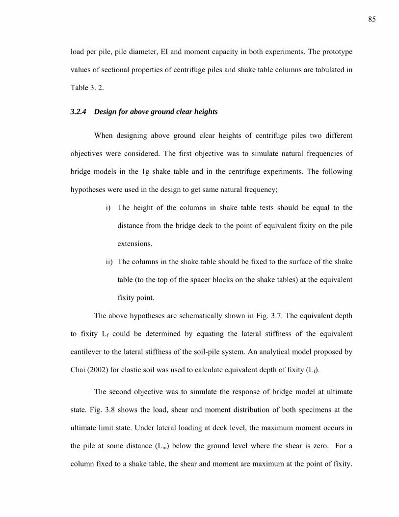
load per pile, pile diameter, EI and moment capacity in both experiments. The prototype
values of sectional properties of centrifuge piles and shake table columns are tabulated in
Table 3. 2.
3.2.4 Design for above ground clear heights
When designing above ground clear heights of centrifuge piles two different
objectives were considered. The first objective was to simulate natural frequencies of
bridge models in the 1g shake table and in the centrifuge experiments. The following
hypotheses were used in the design to get same natural frequency;
i) The height of the columns in shake table tests should be equal to the
distance from the bridge deck to the point of equivalent fixity on the pile
extensions.
ii) The columns in the shake table should be fixed to the surface of the shake
table (to the top of the spacer blocks on the shake tables) at the equivalent
fixity point.
The above hypotheses are schematically shown in Fig. 3.7. The equivalent depth
to fixity Lf could be determined by equating the lateral stiffness of the equivalent
cantilever to the lateral stiffness of the soil-pile system. An analytical model proposed by
Chai (2002) for elastic soil was used to calculate equivalent depth of fixity (Lf).
The second objective was to simulate the response of bridge model at ultimate
state. Fig. 3.8 shows the load, shear and moment distribution of both specimens at the
ultimate limit state. Under lateral loading at deck level, the maximum moment occurs in
the pile at some distance (Lm) below the ground level where the shear is zero. For a
column fixed to a shake table, the shear and moment are maximum at the point of fixity.
85

The approach used in this study was to reasonably simulate shear distribution while
paying more attention to simulate the moment distribution in the 1 g and centrifuge shake
tables. The depth of maximum moment of pile was calculated for linear distribution (Ll)
(see Fig. 3.8). Then the columns on the shake table should be fixed to the surface of the
shake table at a distance Ll below the ground level. According to this logic, Hcol, shake table
= Hclear, pile + Ll. The summary of clear height design at above two scenarios for different
height specimens is shown in Table 3.3. The calculated clear heights based on elastic
response (first objective) are higher than the values for inelastic system response (second
objective). The calculated clear height to match natural frequencies of both models (from
the first objective) was used in the centrifuge tests. Because the research team reasoned
that we would have a better chance of matching the elastic response in the centrifuge and
the 1 g experiments, it was decided to design the models to match the elastic stiffness.
3.2.5 Deck properties and spacing between bents
The superstructure for the shake table specimen was a solid post tensioned,
precast slab. In the centrifuge test, pile head masses (bent caps-made from 6061-T6
aluminum) were connected with light weight aluminum (5052-T6 aluminum) plates. Both
deck models were relatively stiff in the transverse direction so that the interior bent
motion was forced to be essentially equal to the average of the two exterior bents. For the
1 g bridge model, the longitudinal spacing between bents was 37 m in prototype scale.
The longitudinal spacing between bents in the centrifuge test was approximately 15.1 m
in prototype scale to fit the bridge in the container and on the assumption that the spacing
was not critical. This difference in spacing, however, resulted in a different torsional
stiffness of the system for the centrifuge and the 1 g tests.
86
3.2.6 Selection of input motion and testing sequence
The input motions used in the centrifuge and 1 g tests were based on the
Northridge 01/17/94 1231, Century City LACC North, 090 (CMG Station 24389)
earthquake recording. To account for site response effects, estimated free field motion
from site response analysis at the equivalent point of fixity (assumed to be 2.5 m below
the ground surface) was used as the input motion in the 1 g tests. To obtain comparable
results in centrifuge experiments, an exercise was performed prior to the centrifuge tests
to tune the servo hydraulic shakers to produce the same motion at a depth of 2.5 m
(prototype scale) below the ground surface. Time histories and spectral accelerations of
base motions before and after this tuning exercise and the magnitude of the transfer
function used to modify the original base motion are shown in Fig. 3.9. Time histories
and spectral accelerations of the target and achieved free field motions at the equivalent
fixity point (at 50 mm below ground surface in the centrifuge model scale) before and
after the tuning exercise are presented in Fig. 3.10. As shown in Fig. 3.10, the free field
motions were determined to agree reasonably well with the target over a range of periods
between 0.6 s and 1.0 s, which encompasses the natural period of the bridge bents. The
instrumentation details, ground motion sequence and other aspects of centrifuge
experiment are described in test series data report (Ilankatharan et al. 2005).
87
3.3 Comparison of centrifuge and 1g shake table experimental results
3.3.1 During a medium level shaking event (peak base acc=0.25 g in centrifuge test)
Fig. 3.11 compares the acceleration time histories of deck motions in both
experiments. The elastic response spectra of free field soil motions at the equivalent
depth of fixity, shake table from 1g shake table experiments and deck motions from
centrifuge and 1 g experiments are presented in Fig 3.12. The locations of sensors
(accelerometers recorded above data) in the centrifuge and shake table experiments are
shown in Fig. 3.2 and Fig. 3.4. Deck displacements from both experiments are shown in
Fig. 3.13. As shown in the above figures the results are in reasonable agreement for tall
and medium bents. Some differences are apparent in deck motions for short bent. For the
short bent, the shake table deck response shows response peaks of 0.6 and 0.8 s while the
centrifuge shows response peaks at 0.6 and 0.9 s. The observed predominant period of
centrifuge bridge model was approximately 0.9 s while that of shake table model was
approximately 0.7 s. The first two modes of bridge models involved a significant amount
of torsion about a vertical axis. The torsional natural periods will vary with longitudinal
spacing of bents, which, as described earlier, was not scaled accurately in the centrifuge
test (due to limited size of the model container). This explains why the natural periods
were different in the centrifuge and the 1 g shake table experiments (Ranf et al. 2006).
Fig. 3.14 presents the spectral ratio of deck motions to free field soil motions at 2.5 m (or
shake table base motions). To produce the above figure, for the case with the centrifuge
bridge model, spectral accelerations of deck motions are divided by the spectral
accelerations of free field soil motions at 2.5 m and for the case with the shake table
88
model, spectral accelerations of deck motions are divided by the spectral accelerations of
table motions. The magnitude of spectral ratios varies with frequencies for different bents
in two experiments. This may be explained by the different amount of energy dissipation
by various sources in centrifuge and shake table experiments: such as soil particle-
particle friction and sliding, particle crushing, friction at soil-pile interface, radiation
damping provided by the piles in the soil, pile/column yielding, and radiation damping in
shake table system. In the period range between 0.5 to 1.0 s, the magnitude of spectral
ratios in shake table test is higher than that of centrifuge test. This suggests that the
significant amount of energy dissipation that occurred in centrifuge experiment was not
present in shake table experiment. Fig. 3.15 compares the time histories of bending
strains measured in both experiments in different clear height columns, at 1.3 m below
the deck level. As shown in Fig. 3.15, the frequency contents and time histories of strains
are in reasonable agreement for the tall and the medium bents. However, the
unsymmetrical strain pattern, with spikes in the negative direction, for the reinforced
concrete model columns in the shake table experiment were not observed in centrifuge
experiment.
3.3.2 During a Large level shaking event (peak base acc = 0.78g in centrifuge test)
The elastic response spectra of free field soil motions at the equivalent fixity
point, shake table motions in the 1g tests, and deck motions from 1 g and centrifuge tests
are shown in Fig. 3.16. The peak accelerations of measured free field motions at the
equivalent depth of fixity are almost the same for the short bent and medium bent. A
small difference for the tall bent is likely due to a difference in the depth of the
accelerometers. Peak base accelerations for all three-shake table base motions have
89
noticeable differences; the table motion for the short bent is significantly different from
others. This may be due to the interaction between the short stiff bent and the shake table.
The impact of test specimen-shake table interaction on the measured table motions and
on the bridge system response was discussed by Johnson et al. (2006). It was shown in
their study that the measured shake table motion for short bent was larger than the target
table motion. This discrepancy in the table motion resulted first bent collapse in the short
bent during the experiment. However, the pre-test analyses concluded the first bent
collapse would occur in the medium bent. Fig. 3.17 compares the spectral ratios of deck
motions which were estimated as described earlier for the medium level shaking event.
During this large shaking event, compared to the centrifuge bridge model, the shake table
bridge model shows noticeable reduction (from the case with the medium level shaking)
peak amplitudes of spectral ratios. This may be attributable to the energy dissipation
occurred in the shake table bridge model due to yielding of reinforced concrete columns
during strong shaking.
3.4 Comparison of the system (three-bent) response to the individual bent
response in the centrifuge experiment
As described earlier, the bridge deck in the centrifuge model consisted of a light-
weight aluminum plate bolted to the bridge bents. This afforded the opportunity to first
test each the three bents simultaneously while they were unconnected and then to test
them as a three-bent system.
Fig. 3.18 compares the response spectra of two shaking events. One of these is
the measured base motion for an event with unconnected bents and the other is the input
motion for the case when the bents were connected by the bridge deck. It may be seen
90
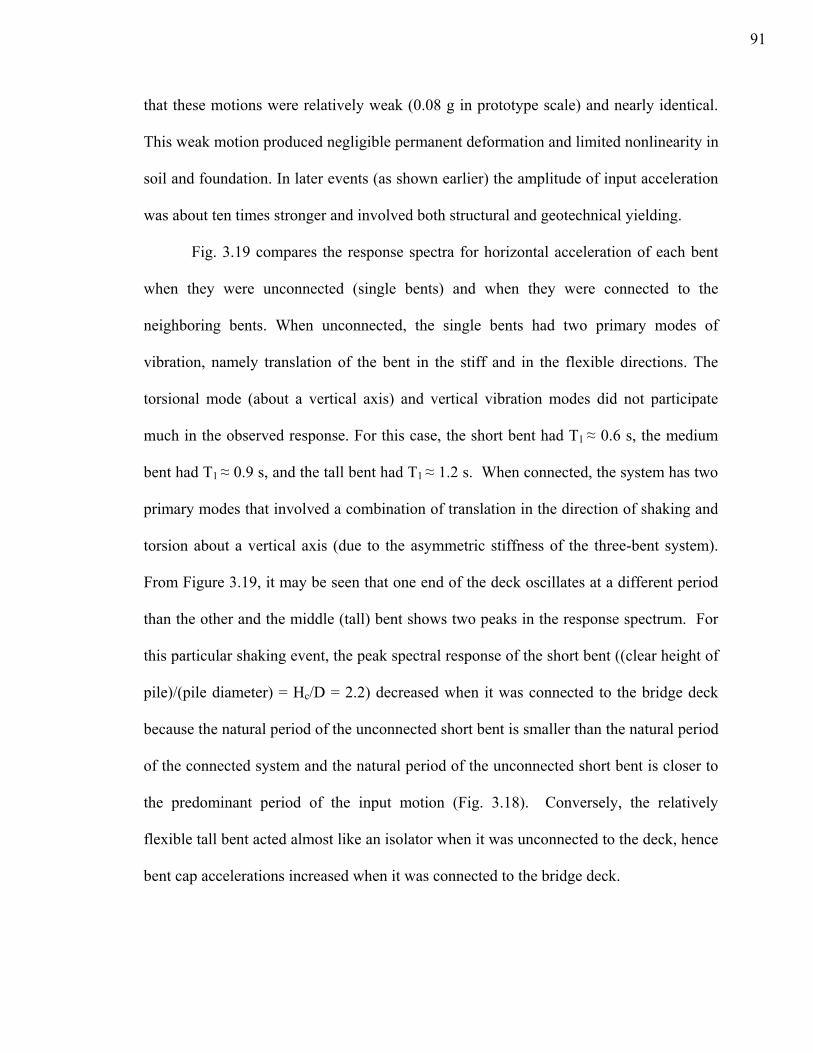
that these motions were relatively weak (0.08 g in prototype scale) and nearly identical.
This weak motion produced negligible permanent deformation and limited nonlinearity in
soil and foundation. In later events (as shown earlier) the amplitude of input acceleration
was about ten times stronger and involved both structural and geotechnical yielding.
Fig. 3.19 compares the response spectra for horizontal acceleration of each bent
when they were unconnected (single bents) and when they were connected to the
neighboring bents. When unconnected, the single bents had two primary modes of
vibration, namely translation of the bent in the stiff and in the flexible directions. The
torsional mode (about a vertical axis) and vertical vibration modes did not participate
much in the observed response. For this case, the short bent had T1 ≈ 0.6 s, the medium
bent had T1 ≈ 0.9 s, and the tall bent had T1 ≈ 1.2 s. When connected, the system has two
primary modes that involved a combination of translation in the direction of shaking and
torsion about a vertical axis (due to the asymmetric stiffness of the three-bent system).
From Figure 3.19, it may be seen that one end of the deck oscillates at a different period
than the other and the middle (tall) bent shows two peaks in the response spectrum. For
this particular shaking event, the peak spectral response of the short bent ((clear height of
pile)/(pile diameter) = Hc/D = 2.2) decreased when it was connected to the bridge deck
because the natural period of the unconnected short bent is smaller than the natural period
of the connected system and the natural period of the unconnected short bent is closer to
the predominant period of the input motion (Fig. 3.18). Conversely, the relatively
flexible tall bent acted almost like an isolator when it was unconnected to the deck, hence
bent cap accelerations increased when it was connected to the bridge deck.
91
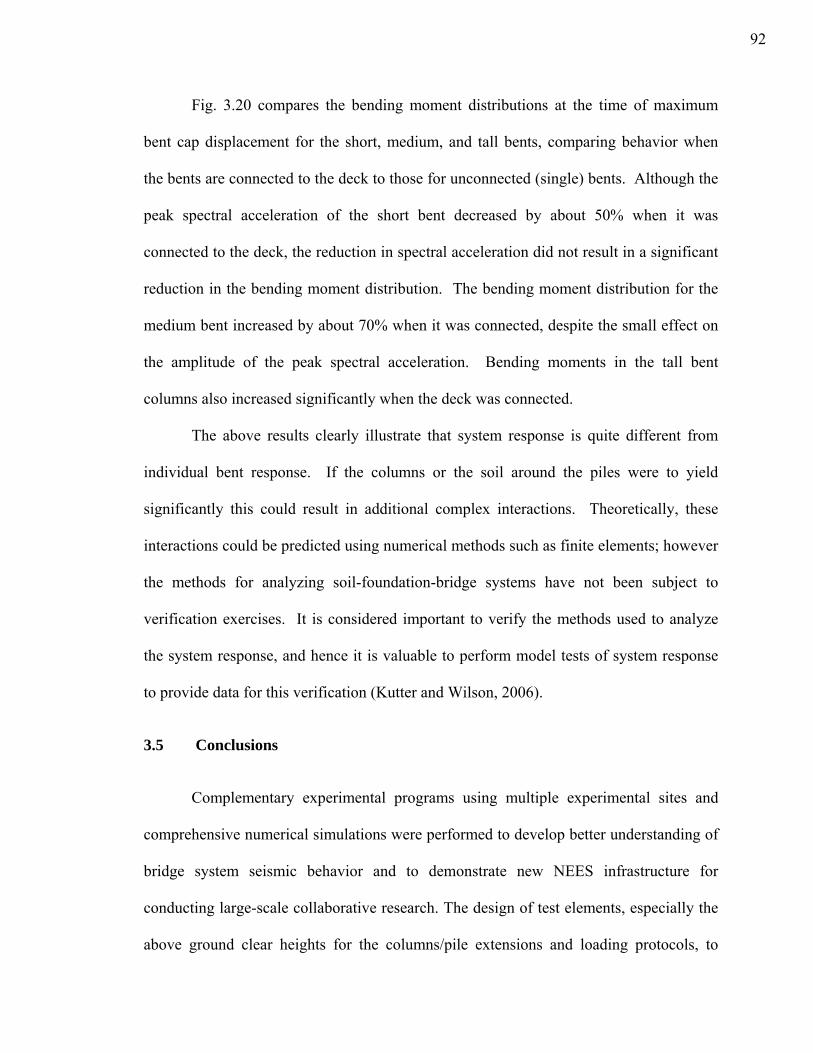
Fig. 3.20 compares the bending moment distributions at the time of maximum
bent cap displacement for the short, medium, and tall bents, comparing behavior when
the bents are connected to the deck to those for unconnected (single) bents. Although the
peak spectral acceleration of the short bent decreased by about 50% when it was
connected to the deck, the reduction in spectral acceleration did not result in a significant
reduction in the bending moment distribution. The bending moment distribution for the
medium bent increased by about 70% when it was connected, despite the small effect on
the amplitude of the peak spectral acceleration. Bending moments in the tall bent
columns also increased significantly when the deck was connected.
The above results clearly illustrate that system response is quite different from
individual bent response. If the columns or the soil around the piles were to yield
significantly this could result in additional complex interactions. Theoretically, these
interactions could be predicted using numerical methods such as finite elements; however
the methods for analyzing soil-foundation-bridge systems have not been subject to
verification exercises. It is considered important to verify the methods used to analyze
the system response, and hence it is valuable to perform model tests of system response
to provide data for this verification (Kutter and Wilson, 2006).
3.5 Conclusions
Complementary experimental programs using multiple experimental sites and
comprehensive numerical simulations were performed to develop better understanding of
bridge system seismic behavior and to demonstrate new NEES infrastructure for
conducting large-scale collaborative research. The design of test elements, especially the
above ground clear heights for the columns/pile extensions and loading protocols, to
92
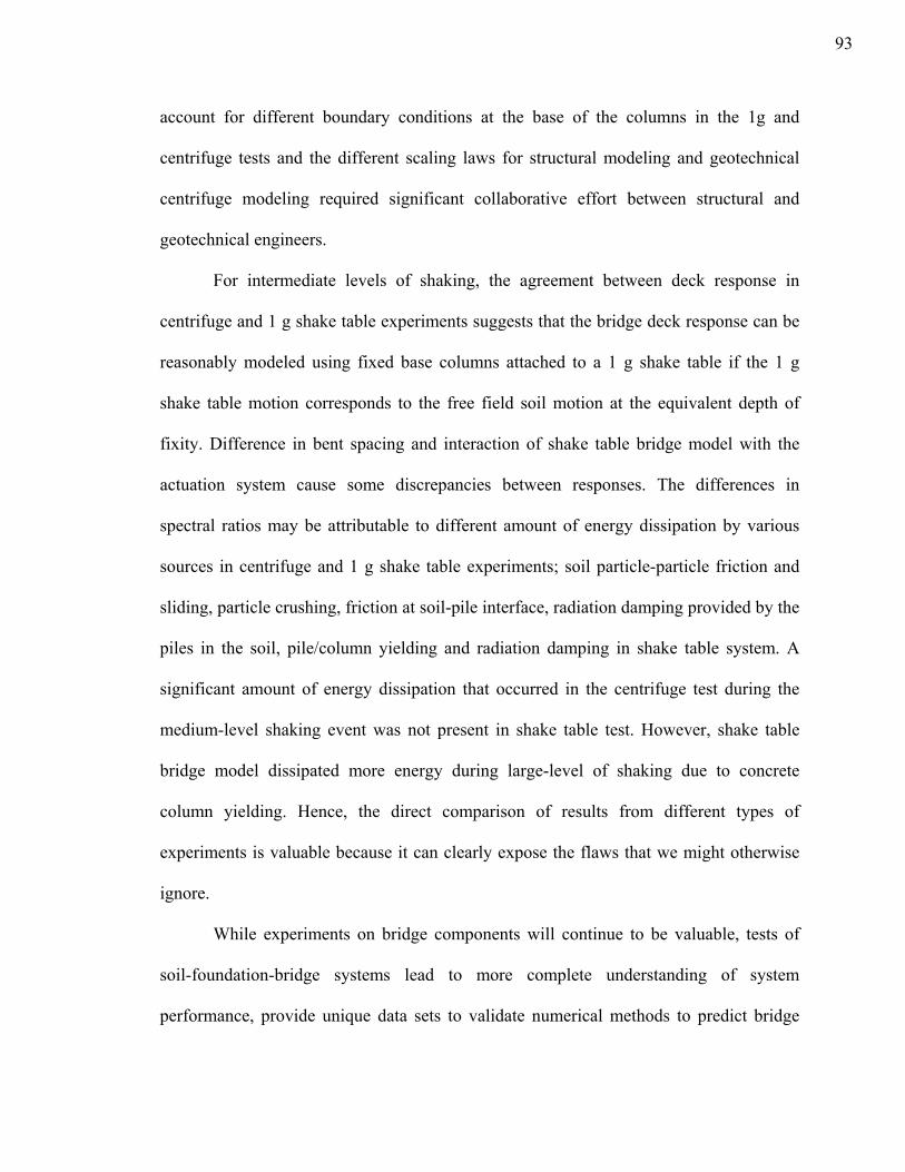
account for different boundary conditions at the base of the columns in the 1g and
centrifuge tests and the different scaling laws for structural modeling and geotechnical
centrifuge modeling required significant collaborative effort between structural and
geotechnical engineers.
For intermediate levels of shaking, the agreement between deck response in
centrifuge and 1 g shake table experiments suggests that the bridge deck response can be
reasonably modeled using fixed base columns attached to a 1 g shake table if the 1 g
shake table motion corresponds to the free field soil motion at the equivalent depth of
fixity. Difference in bent spacing and interaction of shake table bridge model with the
actuation system cause some discrepancies between responses. The differences in
spectral ratios may be attributable to different amount of energy dissipation by various
sources in centrifuge and 1 g shake table experiments; soil particle-particle friction and
sliding, particle crushing, friction at soil-pile interface, radiation damping provided by the
piles in the soil, pile/column yielding and radiation damping in shake table system. A
significant amount of energy dissipation that occurred in the centrifuge test during the
medium-level shaking event was not present in shake table test. However, shake table
bridge model dissipated more energy during large-level of shaking due to concrete
column yielding. Hence, the direct comparison of results from different types of
experiments is valuable because it can clearly expose the flaws that we might otherwise
ignore.
While experiments on bridge components will continue to be valuable, tests of
soil-foundation-bridge systems lead to more complete understanding of system
performance, provide unique data sets to validate numerical methods to predict bridge
93
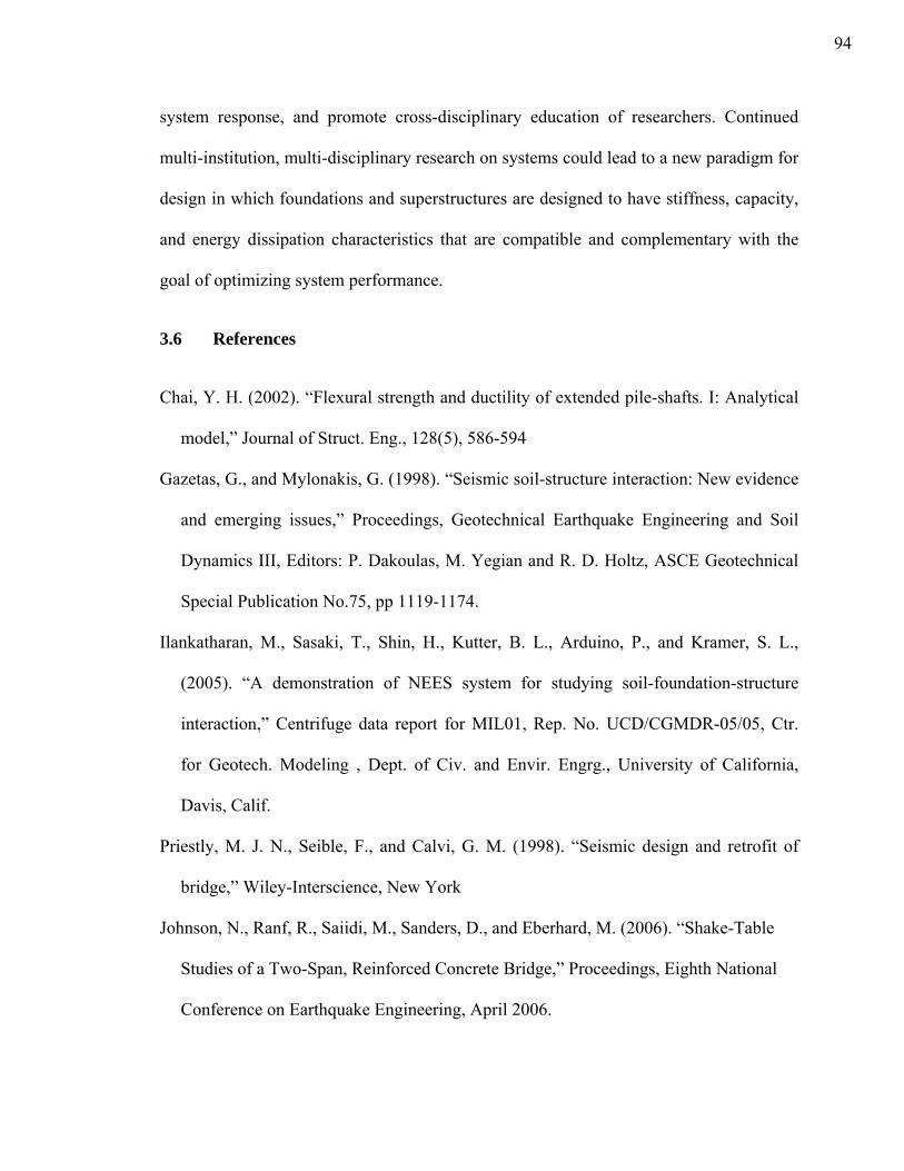
system response, and promote cross-disciplinary education of researchers. Continued
multi-institution, multi-disciplinary research on systems could lead to a new paradigm for
design in which foundations and superstructures are designed to have stiffness, capacity,
and energy dissipation characteristics that are compatible and complementary with the
goal of optimizing system performance.
3.6 References
Chai, Y. H. (2002). “Flexural strength and ductility of extended pile-shafts. I: Analytical
model,” Journal of Struct. Eng., 128(5), 586-594
Gazetas, G., and Mylonakis, G. (1998). “Seismic soil-structure interaction: New evidence
and emerging issues,” Proceedings, Geotechnical Earthquake Engineering and Soil
Dynamics III, Editors: P. Dakoulas, M. Yegian and R. D. Holtz, ASCE Geotechnical
Special Publication No.75, pp 1119-1174.
Ilankatharan, M., Sasaki, T., Shin, H., Kutter, B. L., Arduino, P., and Kramer, S. L.,
(2005). “A demonstration of NEES system for studying soil-foundation-structure
interaction,” Centrifuge data report for MIL01, Rep. No. UCD/CGMDR-05/05, Ctr.
for Geotech. Modeling , Dept. of Civ. and Envir. Engrg., University of California,
Davis, Calif.
Priestly, M. J. N., Seible, F., and Calvi, G. M. (1998). “Seismic design and retrofit of
bridge,” Wiley-Interscience, New York
Johnson, N., Ranf, R., Saiidi, M., Sanders, D., and Eberhard, M. (2006). “Shake-Table
Studies of a Two-Span, Reinforced Concrete Bridge,” Proceedings, Eighth National
Conference on Earthquake Engineering, April 2006.
94
Johnson, N., Saiidi, M., and Sanders, D. (2006). “Large-scale Experimental and
Analytical Seismic Studies of a Two-span Reinforced Concrete Bridge System,” Rep.
No. CCEER-06-02, Ctr. for Civil Engineering and Earthquake Research, Dept. of Civ.
and Envir. Engrg. University of Nevada, Reno, Nevada.
Wood, S.L., Anagnos, T., Arduino, A., Eberhard, M.O., Fenves, G.L., Finholt, T.A.,
Futrelle, J.M., Jeremic, B., Kramer, S.L., Kutter, B.L., Matamoros, A.B., McMullin,
K.M., Ramirez, J.A., Rathje, E.M., Saiidi, M., Sanders, D.H., Stokoe, K.H. and
Wilson, D.W. (2004) "Using NEES to Investigate Soil-Foundation-Structure
Interaction," Proceedings, 13th World Conference on Earthquake Engineering, Paper
2344, Vancouver, Canada, August 1-6.
95
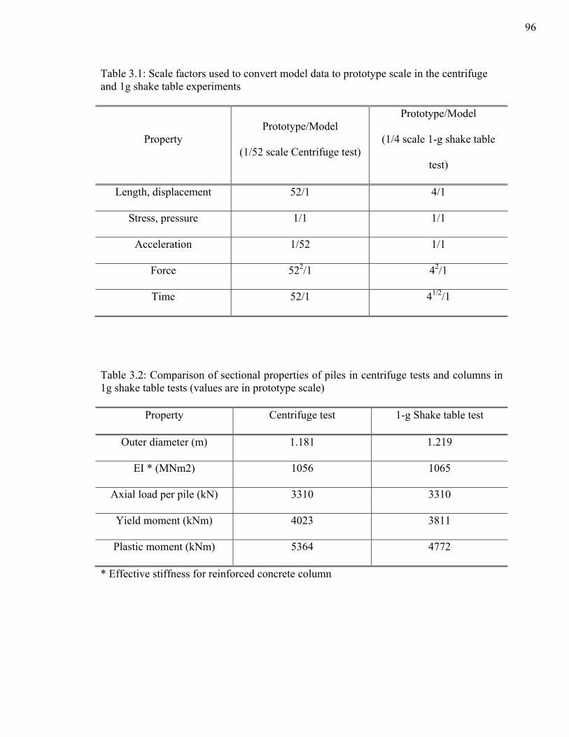
Table 3.1: Scale factors used to convert model data to prototype scale in the centrifuge and 1g shake table experiments
Property Prototype/Model
(1/52 scale Centrifuge test)
Prototype/Model
(1/4 scale 1-g shake table
test)
Length, displacement 52/1 4/1
Stress, pressure 1/1 1/1
Acceleration 1/52 1/1
Force 522/1 42/1
Time 52/1 41/2/1
Table 3.2: Comparison of sectional properties of piles in centrifuge tests and columns in 1g shake table tests (values are in prototype scale)
Property Centrifuge test 1-g Shake table test
Outer diameter (m) 1.181 1.219
EI * (MNm2) 1056 1065
Axial load per pile (kN) 3310 3310
Yield moment (kNm) 4023 3811
Plastic moment (kNm) 5364 4772
* Effective stiffness for reinforced concrete column
96
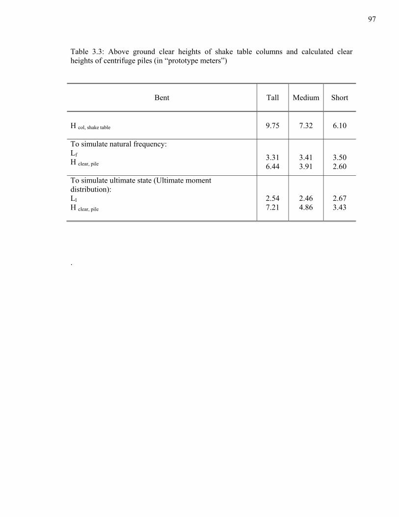
Table 3.3: Above ground clear heights of shake table columns and calculated clear heights of centrifuge piles (in “prototype meters”)
Bent
Tall
Medium
Short
H col, shake table
9.75 7.32 6.10
To simulate natural frequency: Lf H clear, pile
3.31 6.44
3.41 3.91
3.50 2.60
To simulate ultimate state (Ultimate moment distribution): Ll H clear, pile
2.54 7.21
2.46 4.86
2.67 3.43
.
97
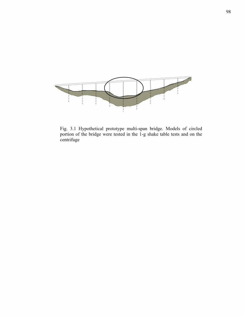
Fig. 3.1 Hypothetical prototype multi-span bridge. Models of circled portion of the bridge were tested in the 1-g shake table tests and on the centrifuge
98
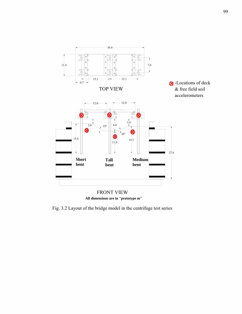
-Locations of deck & free field soil accelerometers
36.4
2.6 6.4
20°
23°
12.0 12.0
15.1 15.1
7.6
15.6
TOP VIEW
FRONT VIEW
Shortbent
All dimensions are in "prototype m"
11.814.3
27.8
11.4
6.7
Tallbent
Mediumbent
3.9
Fig. 3.2 Layout of bridge model in centrifuge test series
Fig. 3.2 Layout of the bridge model in the centrifuge test series
99
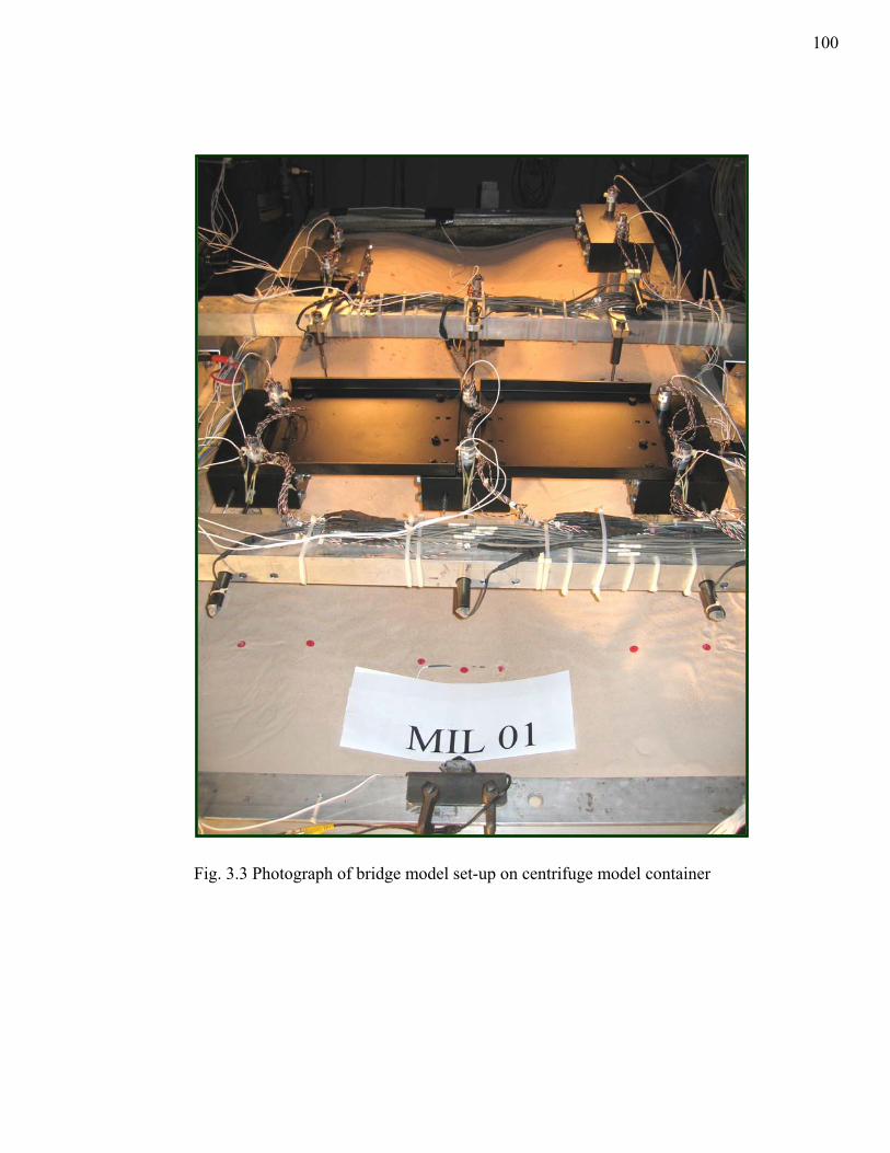
Fig. 3.3 Photograph of bridge model set-up on centrifuge model container
100
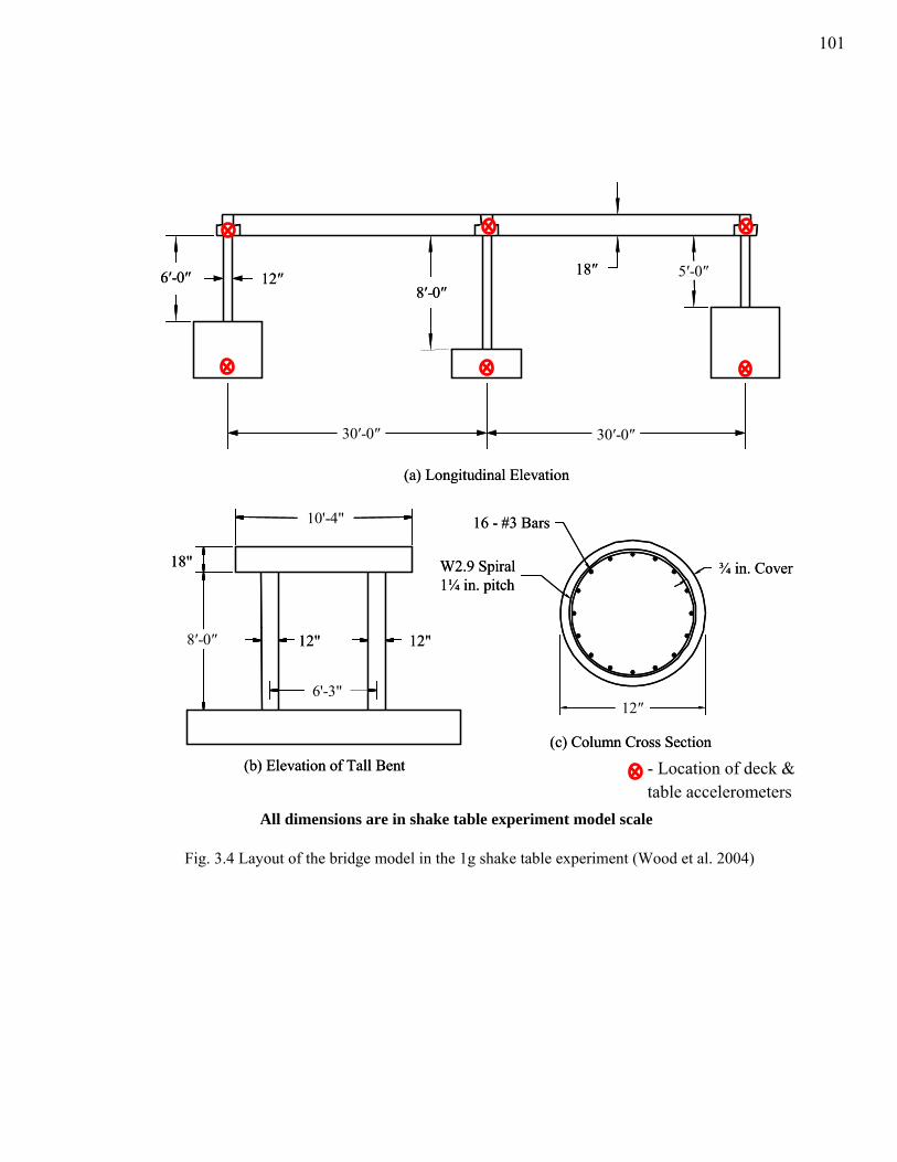
Fig. 3.4 Layout of the bridge model in the 1g shake table experiment (Wood et al. 2004)
6′-0″ 12″8′-0″
5′-0″
30′-0″ 30′-0″
18″
(a) Longitudinal Elevation
10'-4"
8′-0″
18"
6'-3"
12" 12"
(b) Elevation of Tall Bent
16 - #3 Bars
12″
¾ in. CoverW2.9 Spiral1¼ in. pitch
(c) Column Cross Section
6′-0″ 12″8′-0″
5′-0″
30′-0″ 30′-0″
18″
(a) Longitudinal Elevation
10'-4"
8′-0″
18"
6'-3"
12" 12"
(b) Elevation of Tall Bent
16 - #3 Bars
12″
¾ in. CoverW2.9 Spiral1¼ in. pitch
(c) Column Cross Section
- Location of deck & table accelerometers
All dimensions are in shake table experiment model scale
101
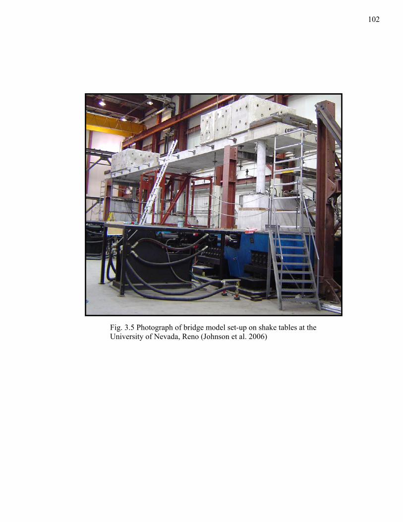
Fig. 3.5 Photograph of bridge model set-up on shake tables at the University of Nevada, Reno (Johnson et al. 2006)
102
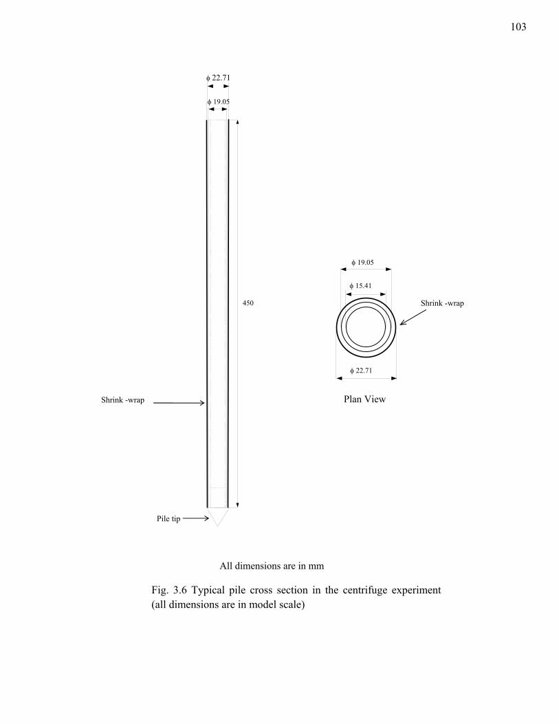
Fig. 3.6 Typical pile cross section in the centrifuge experiment (all dimensions are in model scale)
450
Pile tip
φ 22.71
φ 19.05
Plan View
φ 22.71
φ 15.41
φ 19.05
Shrink -wrap
Shrink -wrap
All dimensions are in mm
103
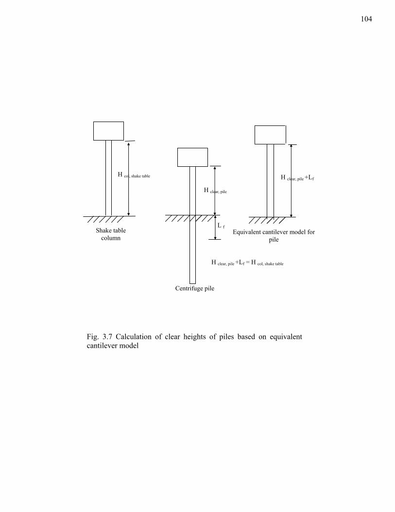
Fig. 3.7 Calculation of clear heights of piles based on equivalent cantilever model
Shake table column
Centrifuge pile
H col, shake table
H clear, pile
L f Equivalent cantilever model for
pile
H clear, pile +Lf = H col, shake table
H clear, pile +Lf
104
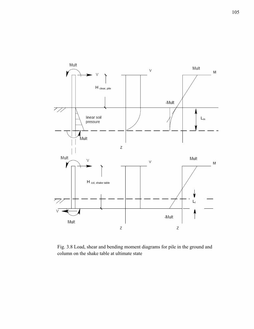
H clear, pile
H col, shake table
Lm
Ll
Fig. 3.8 Load, shear and bending moment diagrams for pile in the ground and column on the shake table at ultimate state
105
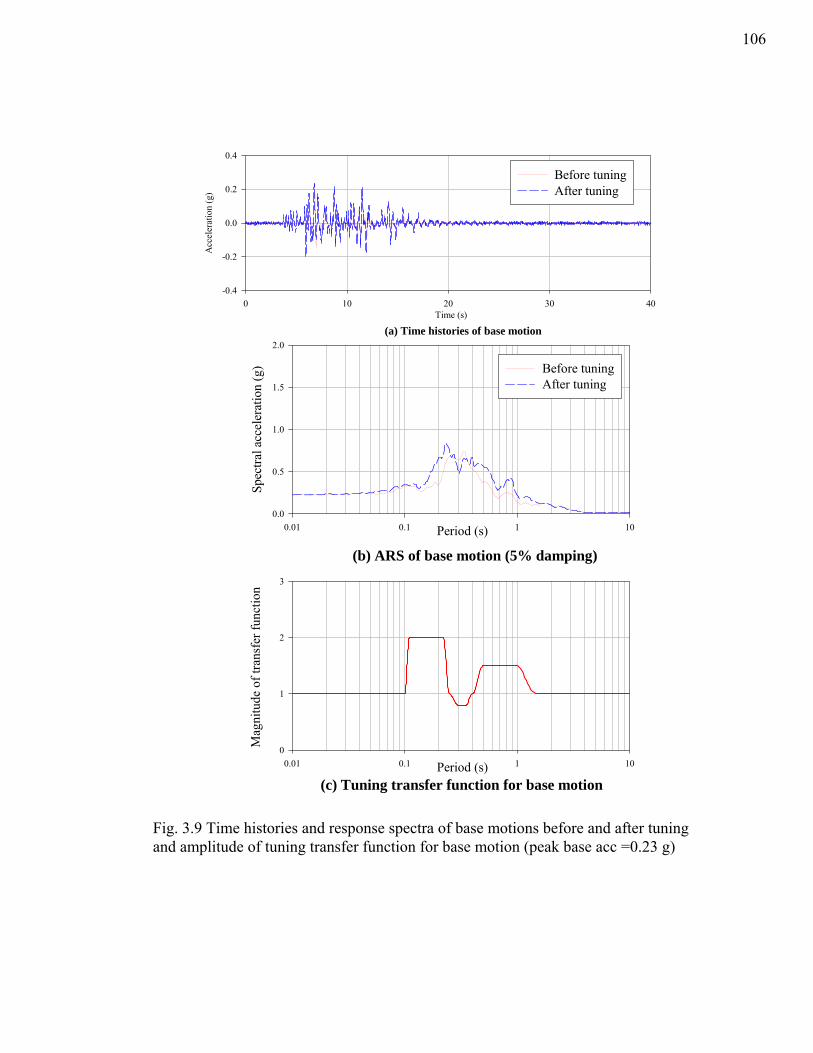
(a) Time histories of base motionTime (s)
0 10 20 30 40
Acc
eler
atio
n (g
)
-0.4
-0.2
0.0
0.2
0.4
Before tuningAfter tuning
(b) ARS of base motion (5% damping)
Period (s)0.01 0.1 1 10
Spec
tral a
ccel
erat
ion
(g)
0.0
0.5
1.0
1.5
2.0
(c) Tuning transfer function for base motionPeriod (s)0.01 0.1 1 10
Mag
nitu
de o
f tra
nsfe
r fun
ctio
n
0
1
2
3
Before tuningAfter tuning
Fig. 3.9 Time histories and response spectra of base motions before and after tuning and amplitude of tuning transfer function for base motion (peak base acc =0.23 g)
106
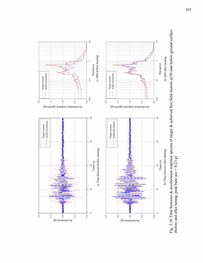
a) T
ime
hist
orie
s bef
ore
tunn
ing
010
2030
40
Acceleration (g) -0.4
-0.20.0
0.2
0.4
Tim
e (s
)
Targ
et m
otio
nA
chie
ved
mot
ion
b) T
ime
hist
orie
s afte
r tun
ning
Tim
e (s
)0
1020
3040
Acceleration (g) -0.4
-0.20.0
0.2
0.4
Targ
et m
otio
nA
chie
ved
mot
ion
c) A
RS
befo
re tu
nnin
gPe
riod
(s)
0.01
0.1
110
Acceleration response spectra (g)
0.0
0.5
1.0
1.5
2.0
Targ
et m
otio
nA
chie
ved
mot
ion
d) A
RS
afte
r tun
ning
Perio
d (s
)0.
010.
11
10Acceleration response spectra (g)
0.0
0.5
1.0
1.5
2.0
Targ
et m
otio
nA
chie
ved
mot
ion
Fig.
3.1
0 Ti
me
hist
orie
s & a
ccel
erat
ion
resp
onse
spec
tra o
f tar
get &
ach
ieve
d fr
ee fi
eld
mot
ion
@50
mm
bel
ow g
roun
d su
rfac
e (b
efor
e an
d af
ter t
unin
g, p
eak
base
acc
= 0
.23
g)
107
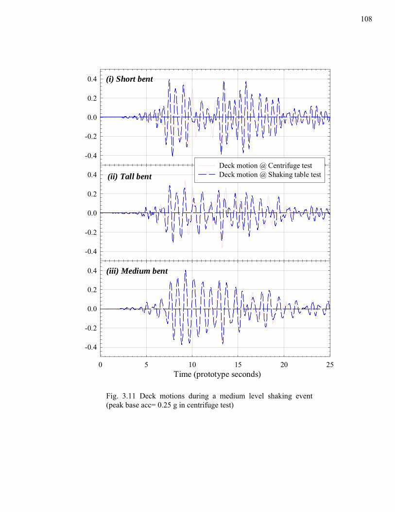
0 5 10 15 20 25
-0.4
-0.2
0.0
0.2
0.4
-0.4
-0.2
0.0
0.2
0.4
-0.4
-0.2
0.0
0.2
0.4
Deck motion @ Centrifuge testDeck motion @ Shaking table test
(i) Short bent
(ii) Tall bent
(iii) Medium bent
Time (prototype seconds)
Fig. 3.11 Deck motions during a medium level shaking event (peak base acc= 0.25 g in centrifuge test)
108
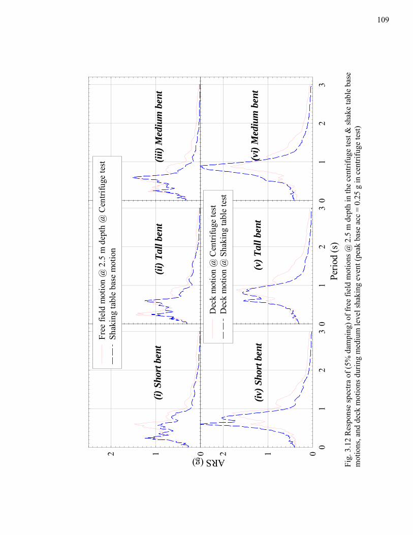
01
23
Perio
d (s
)0
12
3
ARS (g) 012Fr
ee fi
eld
mot
ion
@ 2
.5 m
dep
th @
Cen
trifu
ge te
stSh
akin
g ta
ble
base
mot
ion
01
23
012D
eck
mot
ion
@ C
entri
fuge
test
Dec
k m
otio
n @
Sha
king
tabl
e te
st
(i) S
hort
bent
(ii)
Tall
bent
(vi)
Med
ium
ben
t (i
v) S
hort
bent
(v) T
all b
ent
(iii)
Med
ium
ben
t
Fig.
3.1
2 R
espo
nse
spec
tra o
f (5%
dam
ping
) of f
ree
field
mot
ions
@ 2
.5 m
dep
th in
the
cent
rifug
e te
st &
shak
e ta
ble
base
m
otio
ns, a
nd d
eck
mot
ions
dur
ing
med
ium
leve
l sha
king
eve
nt (p
eak
base
acc
= 0
.25
g in
cen
trifu
ge te
st)
109
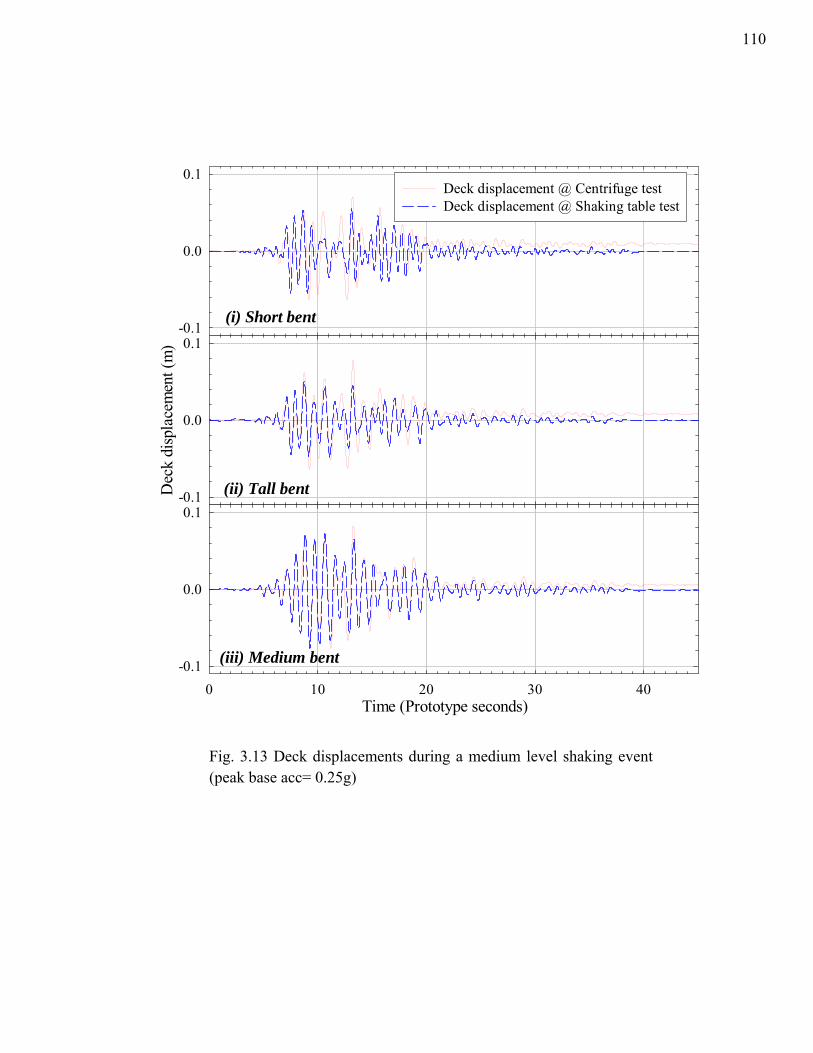
-0.1
0.0
0.1Deck displacement @ Centrifuge testDeck displacement @ Shaking table test
Dec
k di
spla
cem
ent (
m)
-0.1
0.0
0.1
(i) Short bent
Time (Prototype seconds)0 10 20 30 40
-0.1
0.0
0.1(ii) Tall bent
(iii) Medium bent
Fig. 3.13 Deck displacements during a medium level shaking event (peak base acc= 0.25g)
110
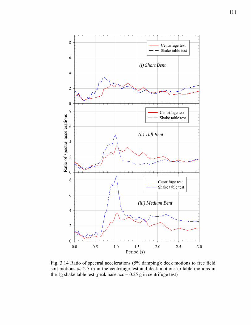
Period (s)
Rat
io o
f spe
ctra
l acc
eler
atio
ns
0
2
4
6
8 Centrifuge testShake table test
0
2
4
6
8
0.0 0.5 1.0 1.5 2.0 2.5 3.00
2
4
6
8
(i) Short Bent
(ii) Tall Bent
(iii) Medium Bent
Centrifuge testShake table test
Centrifuge testShake table test
Fig. 3.14 Ratio of spectral accelerations (5% damping): deck motions to free field soil motions @ 2.5 m in the centrifuge test and deck motions to table motions in the 1g shake table test (peak base acc = 0.25 g in centrifuge test)
111
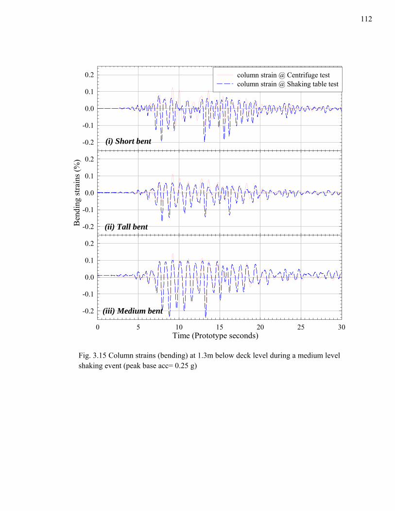
-0.2
-0.1
0.0
0.1
0.2 column strain @ Centrifuge testcolumn strain @ Shaking table test
Ben
ding
stra
ins (
%)
-0.2
-0.1
0.0
0.1
0.2
(i) Short bent
Time (Prototype seconds)0 5 10 15 20 25 30
-0.2
-0.1
0.0
0.1
0.2
(ii) Tall bent
(iii) Medium bent
Fig. 3.15 Column strains (bending) at 1.3m below deck level during a medium level shaking event (peak base acc= 0.25 g)
112
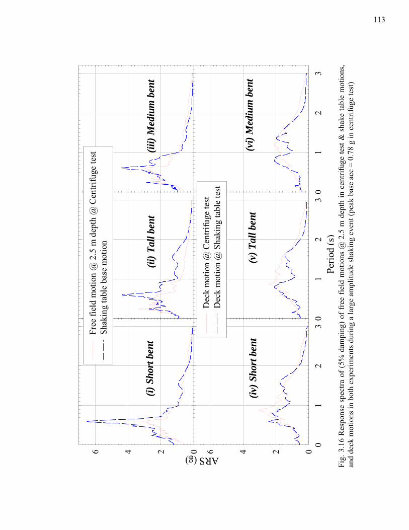
01
23
Perio
d (s
)0
12
3
ARS (g) 0246Fr
ee fi
eld
mot
ion
@ 2
.5 m
dep
th @
Cen
trifu
ge te
stSh
akin
g ta
ble
base
mot
ion
01
23
0246D
eck
mot
ion
@ C
entri
fuge
test
Dec
k m
otio
n @
Sha
king
tabl
e te
st
(i) S
hort
bent
(ii)
Tall
bent
(vi)
Med
ium
ben
t (i
v) S
hort
ben
t (v
) Tal
l ben
t
(iii)
Med
ium
ben
t
Fig.
3.1
6 R
espo
nse
spec
tra o
f (5%
dam
ping
) of f
ree
field
mot
ions
@ 2
.5 m
dep
th in
cen
trifu
ge te
st &
sha
ke ta
ble
mot
ions
, an
d de
ck m
otio
ns in
bot
h ex
perim
ents
dur
ing
a la
rge
ampl
itude
shak
ing
even
t (pe
ak b
ase
acc
= 0.
78 g
in c
entri
fuge
test
)
113
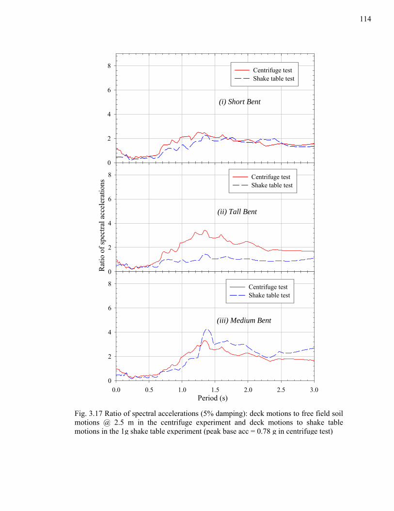
Period (s)
Rat
io o
f spe
ctra
l acc
eler
atio
ns
0
2
4
6
8Centrifuge testShake table test
0
2
4
6
8
0.0 0.5 1.0 1.5 2.0 2.5 3.00
2
4
6
8
(i) Short Bent
(ii) Tall Bent
(iii) Medium Bent
Centrifuge testShake table test
Centrifuge testShake table test
Fig. 3.17 Ratio of spectral accelerations (5% damping): deck motions to free field soil motions @ 2.5 m in the centrifuge experiment and deck motions to shake table motions in the 1g shake table experiment (peak base acc = 0.78 g in centrifuge test)
114
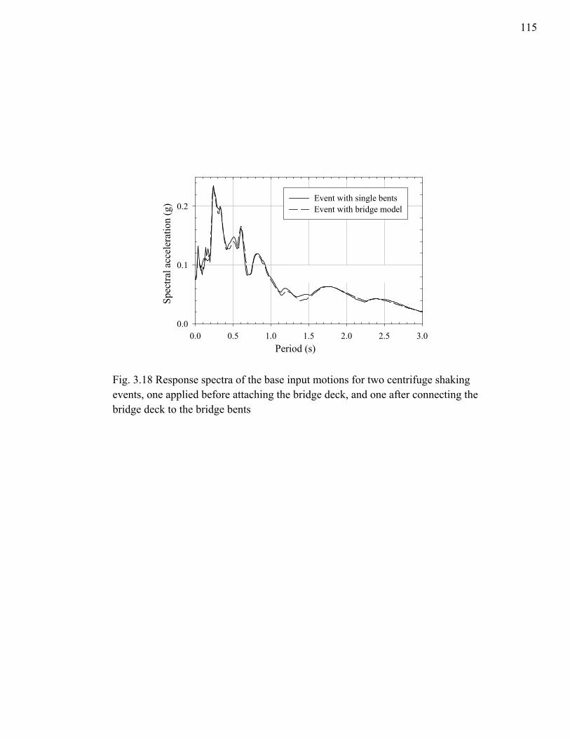
Fig. 3.18 Response spectra of the base input motions for two centrifuge shaking events, one applied before attaching the bridge deck, and one after connecting the bridge deck to the bridge bents
Period (s)0.0 0.5 1.0 1.5 2.0 2.5 3.0
Spec
tral a
ccel
erat
ion
(g)
0.0
0.1
0.2Event with single bentsEvent with bridge model
(i) Short Bent (Hc/D=2.2)
115
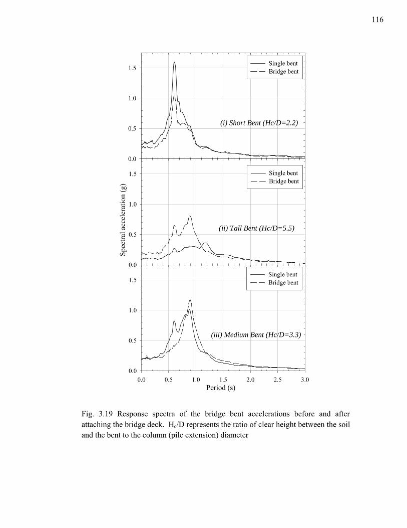
Period (s)
Spec
tral a
ccel
erat
ion
(g)
0.0
0.5
1.0
1.5Single bentBridge bent
0.0
0.5
1.0
1.5
0.0 0.5 1.0 1.5 2.0 2.5 3.00.0
0.5
1.0
1.5
Single bentBridge bent
Single bentBridge bent
(i) Short Bent (Hc/D=2.2)
(ii) Tall Bent (Hc/D=5.5)
(iii) Medium Bent (Hc/D=3.3)
Fig. 3.19 Response spectra of the bridge bent accelerations before and after attaching the bridge deck. Hc/D represents the ratio of clear height between the soil and the bent to the column (pile extension) diameter
116
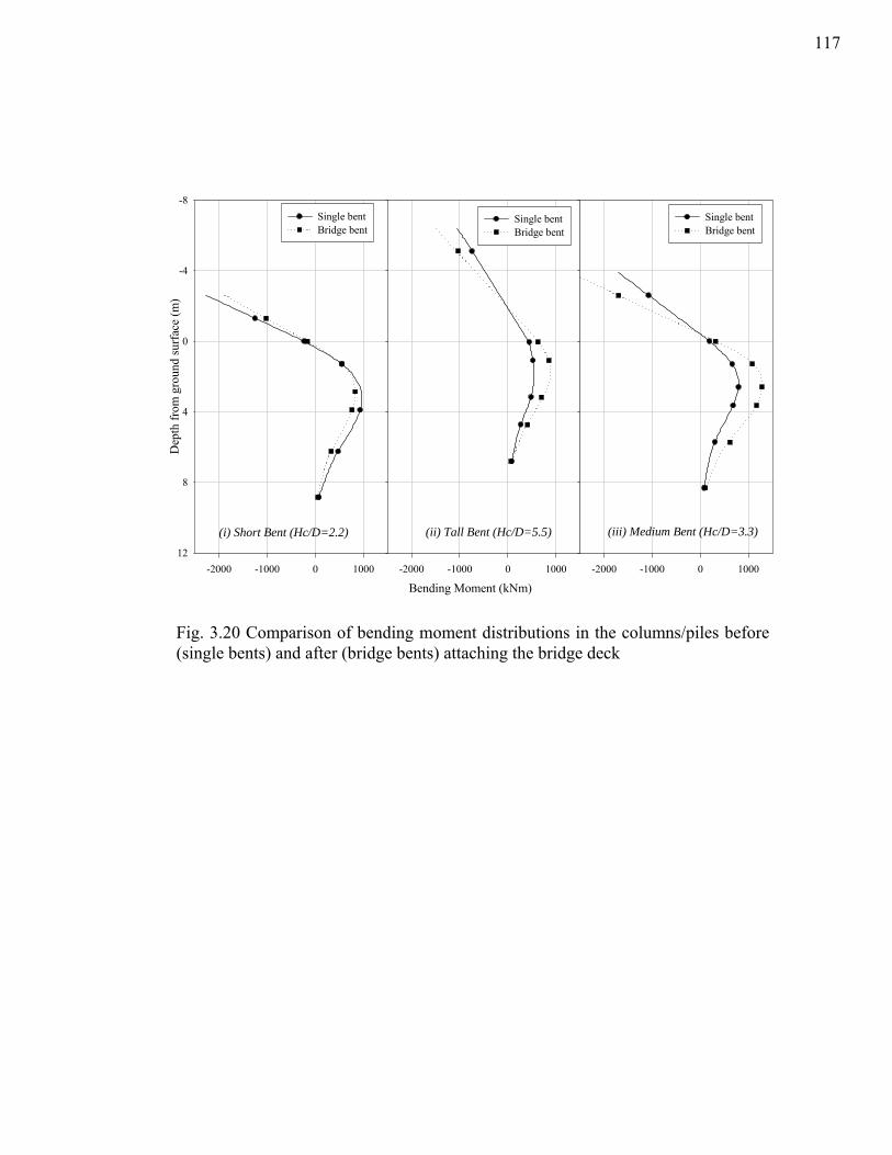
Bending Moment (kNm)-2000 -1000 0 1000
Dep
th fr
om g
roun
d su
rfac
e (m
)
-8
-4
0
4
8
12-2000 -1000 0 1000 -2000 -1000 0 1000
(i) Short Bent (Hc/D=2.2) (ii) Tall Bent (Hc/D=5.5) (iii) Medium Bent (Hc/D=3.3)
Single bentBridge bent
Single bentBridge bent
Single bentBridge bent
Fig. 3.20 Comparison of bending moment distributions in the columns/piles before (single bents) and after (bridge bents) attaching the bridge deck
117
Chapter 4
Modeling input motion boundary conditions for simulations of
geotechnical shaking table tests
The chapter discusses effects of using different input motion boundary conditions
on the sensitivity of numerical simulations results to errors in material properties of a soil
model tested on a centrifuge shaking table. This chapter is a journal paper which has been
submitted for publication in the Professional journal of the Earthquake Engineering
Research Institute (EERI). The complete reference of the paper is given below.
Ilankatharan, M., and Kutter, B. L. (2008). “Modeling Input Motion Boundary
Conditions for Simulations of Geotechnical Shaking Table Tests.” Earthquake Spectra,
Earthquake Engineering Research Institute (under review).
118
Abstract: This paper discusses effects of using different input motion boundary
conditions on the sensitivity of numerical simulations results to errors in material
properties of a specimen tested on a shaking table. In the flexible-actuator-prescribed-
force boundary condition, seismic input is specified by a force across an actuator element
that drives the shaking table; hence, the boundary between the test specimen and the
shaking table is an absorbing-base boundary across which energy may be transferred. In
the prescribed-displacement boundary condition, the measured shaking table motion in
the experiment is used as a prescribed displacement in the simulation. Numerical
simulations of a hypothetical centrifuge shaking table experiment involving a 1D soil
column are performed to illustrate effects of the above two input motion boundary
conditions. The flexible-actuator-prescribed-force approach generally yielded smaller,
almost constant sensitivities. The prescribed-displacement approach yielded larger and
more variable sensitivities. The observation that the sensitivity of results to errors in
input data depends on the input motion boundary conditions, raises a fundamental
question: How can we assess the significance of a discrepancy between a numerical
simulation and an experimental result? This paper shows that, for shaking table tests, the
significance of errors in the numerical simulations cannot be rigorously assessed without
accounting for dynamic interaction between the test specimen and the actuation system.
119
4.1 Introduction
One of the greatest challenges that earthquake engineers face is the paucity of
data available to calibrate the performance of numerical models for varying earthquake
characteristics (level of shaking, frequency content, and waveform), soil profile
characteristics, and superstructure/substructure characteristics. Dynamic centrifuge
modeling with detailed instrumentation is often used to obtain physical data, gain insight
into the mechanisms involved, and perform parametric studies to calibrate numerical
models. VELACS (VErification of Liquefaction Analyses by Centrifuge Studies) is just
one example of a project where the data from several series of dynamic centrifuge model
tests were used to verify various numerical procedures (Arulanandan et al, 1993).
A geotechnical centrifuge-shaker system includes a soil model, a model container,
a shaking table and its reaction mass as depicted in Fig. 4.1. All of the different
components of dynamic system, with their own resonant frequencies, interact with the
soil model during dynamic excitation, some absorbing energy and others allowing
undesired modes to affect the response observed in the experiment. This interaction of the
soil model and the centrifuge/actuation system might attenuate or exaggerate the
discrepancies in responses of the experiment and the numerical simulation. A
fundamental question then arises: ‘How should we assess the quality of a comparison
between an experiment and a numerical simulation?’ Up to now, comparisons between
theory and experiment have only been qualitative. To answer the fundamental question, it
would be essential to accomplish the following:
i. Identify the model parameters that are being investigated in the experiment and
the simulation,
120
ii. Confirm that the experiment and the numerical simulation are reasonably
sensitive to uncertainties in these model parameters, and
iii. Understand how uncertainties in the model parameters (input) are propagated
through the numerical simulation and through the experiment to the result (output); i.e.,
understand the sensitivity of output to errors in input.
Without understanding the sensitivity of output to input in the experiment and the
simulation, it is not possible to make a rigorous evaluation of the significance of
agreement or disagreement between simulation and experiment. The goal of present study
revolves around one aspect of the fundamental question raised above: To investigate how
the sensitivity of output to changes in input parameters depends on the input motion
boundary conditions assumed in a numerical simulation of a centrifuge shake table
experiment.
In a typical shake table experiment, an actuator command displacement is
specified to a servo controller and the response of the container base is measured as an
output. There is energy transfer (analogous to radiation damping through compliant
boundaries in the field) out of test specimen through the shake table and the reaction
mass (Kutter, 1995). Analogous to 1-D wave propagation in soil layers, the measured
motion at the base of the container, which is a combination of both reflected and
transmitted seismic waves at the base of the container (Fig. 4.2), depends on dynamic
properties of different components of model-shaker system. If the shaking table and
reaction mass were infinitely stiff, all the wave energy generated by the shaker would be
trapped in the soil model and the measured container base motion could be used as “true
input” to a numerical simulation. However, real shaking table tests, especially those in
121
the highly constrained payload of a geotechnical centrifuge involve flexible and finite
masses of shaking table and reaction mass, and the impedance contrast at the base of the
test specimen is not very large, which increases the significance of proper treatment of
the boundary condition.
This paper discusses two different approaches for inputting excitation to a
numerical simulation of a dynamic centrifuge shake table experiment. The first approach
involves more realistic representation of experimental boundary conditions and requires
detailed modeling of different components of model-shaker system. In this approach,
seismic input to simulation model is specified as a force input time history across the
actuator; the motion at the container as well as the response of the soil deposit is
calculated as outputs of the simulation. The boundary between the test specimen and the
shaking table is treated as an absorbing boundary so that the energy transfer out of the
test specimen through the actuator and reaction mass can be accounted for. In the second
approach, the measured shaking table motion is used as a prescribed displacement in the
numerical simulation. This paper presents numerical examples illustrating above two
approaches and results from a series of sensitivity studies using above two approaches.
Further, relative merits of these approaches and the effects of the test specimen-actuation
system interaction on the simulation results are discussed.
4.2 Modeling of a soil column mounted on a centrifuge shaking table
We consider a hypothetical experiment where a soil column, with a height of 1 m
and a cross sectional area of 1 m2, is tested on a centrifuge shaking table. The important
components of the experiment would be similar to the features of a centrifuge shaker
system shown in Fig. 4.1; except for this hypothetical example we assume that the base
122
of the container does not rock, and that the container is mass less and frictionless. An
increased gravitational field of 50 g is considered for the centrifuge experiment and the
corresponding numerical simulations. The dimensions of the finite element domain, all
modeling parameters, and the simulation results are presented in centrifuge model scale
unless otherwise specified. The centrifuge scaling factors for some physical properties are
given in Table 4.1; further details on the centrifuge scaling laws can be found in Kutter
(1992).
4.2.1 Representing input motion boundary conditions
2D finite element models are developed using OpenSees (Open System for
Earthquake Engineering Simulation, Mazzoni et al. 2006) to represent the dynamics of
soil model-shaker system. To improve understanding of interactions among different
components of the dynamic system and to evaluate how the sensitivity of simulation
results depends on the input motion boundary conditions in the simulations, the
boundary conditions are treated with two different levels of detail as described below,
and depicted in Fig. 4.3.
4.2.1.1 Prescribed-force simulation
This simulation model involves realistic representation of experimental boundary
conditions as shown in Fig. 4.3(a). In this approach, the effect of shaker and reaction
mass is included and the flexibility of the actuator is modeled. Excitation to the system is
applied by equal and opposite forces, Fcom(t), across a spring representing the stiffness of
the hydraulic actuator of the centrifuge shake table (as shown in Fig. 4.4). This paper
reserves the phrase “flexible-actuator-prescribed-force boundary condition” to denote the
123
input motion boundary condition corresponding to this approach. In this input motion
boundary condition, the boundary between the soil model and the shaking table is treated
as an “absorbing-boundary” so that the energy transfer out of the soil model through the
shaking table and the reaction mass can be taken into account. The two main outputs
corresponding to the prescribed-force simulation are the motions, which are calculated as
a function of soil shear modulus, G, at the base of the soil column ab_pf(G) and at the
ground surface as_pf(G), as schematically shown in Fig. 4.3(a).
4.2.1.2 Prescribed-displacement simulation
In this suite of analysis, the effect of shaker and reaction mass is excluded. The
calculated motion at the base of the soil column from the prescribed-force simulation
(ab_pf(G)) is used as a prescribed displacement at the base of the soil column (Fig. 4.3(b)).
The purpose of this suite of analysis is to mimic a simulation model which adapts
measured motion at the base of the soil column from the experiment as an input motion
for dynamic excitation (ab_pd). The main output corresponding to the prescribed-
displacement is the motion, which is calculated as a function of soil shear modulus at the
ground surface as_pd(G), as schematically shown in Fig. 4. 3(b).
4.2.2 Soil model
A 1D shear-beam type FE model is employed to simulate soil site response, where
soil is modeled with 4-node quad elements using two different material models. A linear
elastic nDmaterial (Mazzoni et al. 2006), with a constant shear modulus along the depth
of soil profile, is used in the first series of analysis. The second series of analysis employs
an elasto-plastic plastic constitutive model, PressureDependMultiYield (PDMY). Within
124
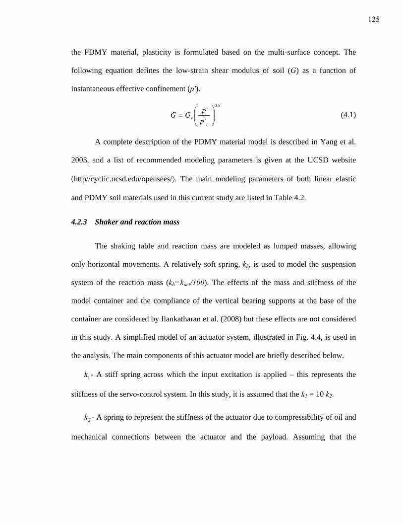
the PDMY material, plasticity is formulated based on the multi-surface concept. The
following equation defines the low-strain shear modulus of soil (G) as a function of
instantaneous effective confinement (p′).
5.0
''⎟⎟⎠
⎞⎜⎜⎝
⎛=
rr p
pGG (4.1)
A complete description of the PDMY material model is described in Yang et al.
2003, and a list of recommended modeling parameters is given at the UCSD website
⟨http//cyclic.ucsd.edu/opensees/⟩. The main modeling parameters of both linear elastic
and PDMY soil materials used in this current study are listed in Table 4.2.
4.2.3 Shaker and reaction mass
The shaking table and reaction mass are modeled as lumped masses, allowing
only horizontal movements. A relatively soft spring, kh, is used to model the suspension
system of the reaction mass (kh=kact/100). The effects of the mass and stiffness of the
model container and the compliance of the vertical bearing supports at the base of the
container are considered by Ilankatharan et al. (2008) but these effects are not considered
in this study. A simplified model of an actuator system, illustrated in Fig. 4.4, is used in
the analysis. The main components of this actuator model are briefly described below.
1k - A stiff spring across which the input excitation is applied – this represents the
stiffness of the servo-control system. In this study, it is assumed that the k1 = 10 k2.
2k - A spring to represent the stiffness of the actuator due to compressibility of oil and
mechanical connections between the actuator and the payload. Assuming that the
125
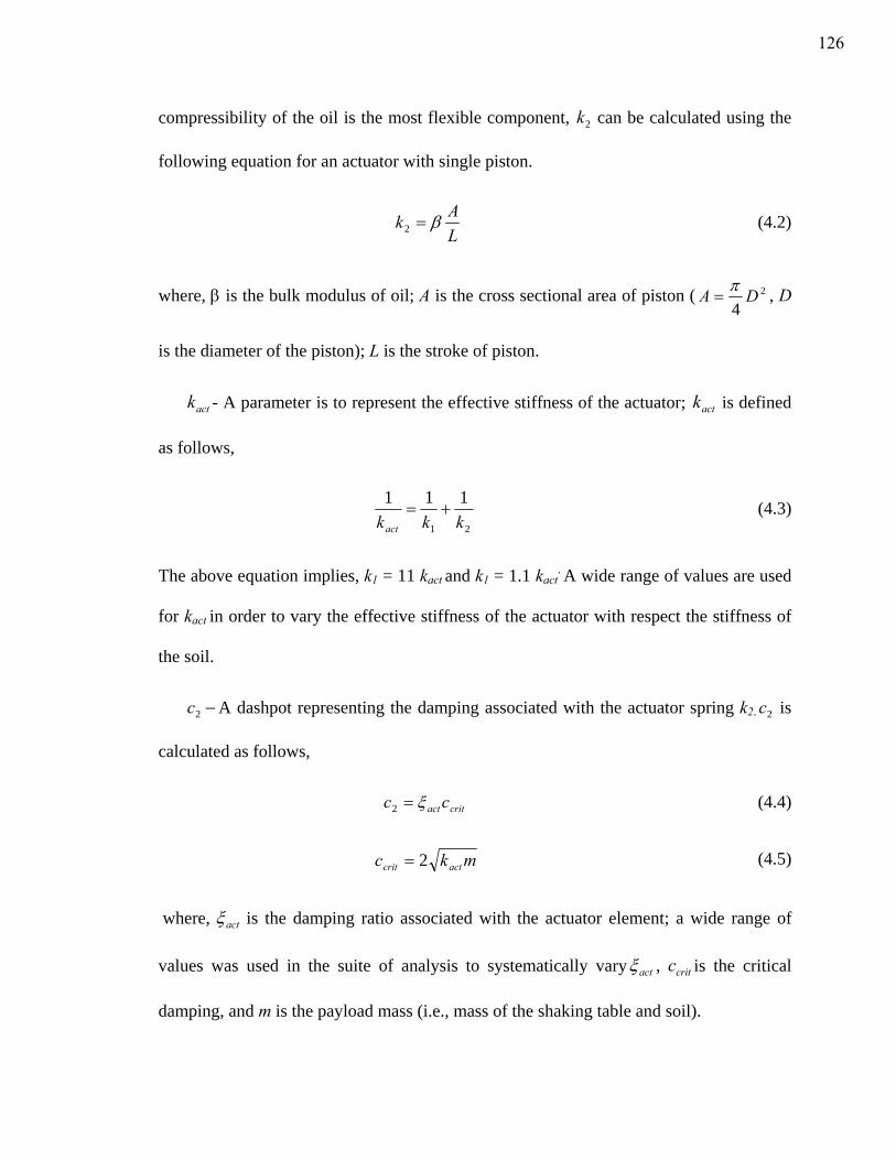
compressibility of the oil is the most flexible component, 2k can be calculated using the
following equation for an actuator with single piston.
LAk β=2 (4.2)
where, β is the bulk modulus of oil; A is the cross sectional area of piston ( 2
4DA π
= , D
is the diameter of the piston); L is the stroke of piston.
actk - A parameter is to represent the effective stiffness of the actuator; actk is defined
as follows,
21
111kkkact
+= (4.3)
The above equation implies, k1 = 11 kact and k1 = 1.1 kact. A wide range of values are used
for kact in order to vary the effective stiffness of the actuator with respect the stiffness of
the soil.
−2c A dashpot representing the damping associated with the actuator spring k2. 2c is
calculated as follows,
critactcc ξ=2 (4.4)
mkc actcrit 2= (4.5)
where, actξ is the damping ratio associated with the actuator element; a wide range of
values was used in the suite of analysis to systematically vary actξ , critc is the critical
damping, and m is the payload mass (i.e., mass of the shaking table and soil).
126

)(tFcom - Excitation force command to the system. )(tFcom is calculated as follows,
)()( 1 tdktF comcom = (4.6)
where, )(tdcom is the command displacement. Fig. 4.5 shows the time histories of
command acceleration and command displacement used in this study.
4.2.4 Selection of damping parameters and input variables
A wide range of values are chosen for main input parameters of the shaker system
and the damping parameters to characterize the dynamics of the centrifuge-shaker system
for various scenarios. The following non-dimensional groups are formulated with
important input variables of the different components of the shaker system.
HGAkact
/- Ratio between the stiffness of the actuator and the stiffness of soil
RM
soil
MM - Ratio between the mass of soil and mass of reaction mass
ST
soil
MM - Ratio between the mass of soil and mass of shaking table
Both in the simulations involving the linear elastic soil material, and the elasto-
plastic soil material in addition to the hysteric damping generated by the stress-strain
loops of PDMY material, a very small amount of frequency dependent viscous
damping, soilξ , was assigned to the soil column. For the soil damping, a combination of
mass and stiffness proportional damping was employed for the purpose of numerical
stability. The coefficients of stiffness dependent and mass dependent damping matrices
are chosen such that the resultant damping ratio soilξ is roughly constant in the frequency
127
range of interest. Specifically, the damping was set to soilξ =2.5% at the first and third
modal frequencies. An example calculation procedure is illustrated in Fig. 4.6. Table 4.3
lists the range of non-dimensional and damping parameters used in the course of the
numerical simulations.
4.3 Simulation results
A base line case is defined by using a set of damping parameters and input
variables to model a representative centrifuge-shaker system
( ,1/
=HGA
kact ,5.0=RM
soil
MM
,5=ST
soil
MM
ξact=20%, and ξsoil=2.5%). The results of the series
of simulations of the above representative centrifuge-shaker system is presented in this
section.
4.3.1 Linear elastic soil material model simulations
Representative simulation results using the linear elastic soil material model are
presented in Fig. 4.7, in terms of acceleration time histories and response spectra (5%
damping) at the base of the soil column and ground surface, for the prescribed-force and
prescribed-displacement simulations. As shown in Fig. 4.7, if the shear modulus of soil
material is perfectly modeled in the simulation (i.e. assumed shear modulus in simulation
is equal to the actual value listed in Table 4.2, Gassumed/Gactual=1), then the calculated
surface response in the prescribed-displacement simulation is identical to that of the
prescribed-force simulation; the soil properties are perfectly modeled in the simulation,
then the results are independent of the input motion boundary conditions.
128
Next we consider a hypothetical simulation of a soil model for which the shear
modulus assumed in the simulation, Gassumed, is not perfect. For example, assume that
(Gassumed/Gactual=0.64), where Gactual is the actual value of shear modulus of the soil
column. This 36% error in shear modulus corresponds to a 20% error in shear wave
velocity. For this case, prescribed-force simulation assumes the reduced G; but the
original input excitation Fcom(Gactual) is used. Since the base motion for the prescribed-
force simulation depends on the soil properties, the resulting calculated container base
motion has an error caused by the error in assumed shear modulus. For the prescribed-
displacement simulation the same reduced value of G is assumed; and the input is taken
as the base motion at the base of the actual soil column abase(Gactual) calculated by the
prescribed-force simulation, which simulation assumes accurate G (i.e. Gactual), as an
input. Fig. 4.8 shows the simulation results for this scenario, in terms of time histories
and acceleration response spectra (5% damping) of calculated motions at the base of the
soil column and at ground surface. From Fig. 4.8, it is apparent that the results are
different for different boundary conditions. The base motion calculated in the prescribed-
force simulation is quite different from that of the prescribed-displacement simulation.
Calculated surface motions from different simulation models are also significantly
different. Time history of surface motion in the prescribed-displacement simulation
shows the presence of gradually decaying periodic vibration cycles and requires a larger
number of cycles before it stabilizes to zero; but, the surface motion calculated from the
prescribed-force simulation does not show these vibration cycles. Discrepancies in the
spectral accelerations of base motion and surface motion in two boundary conditions are
significant at the vicinity of fundamental periods of soil column. For instance, the
129
response spectrum of calculated base motion in the prescribed-force simulation shows
reductions around 0.025 sec and 0.008 sec which are natural periods of first and second
vibration modes of soil column. But these reductions in spectral acceleration of base
motion are not possible in the prescribed-force simulation; since the input motion
employed in the prescribed-displacement simulation is not compatible with the shear
modulus of soil assumed in the simulation. Applying this mismatched base motion in the
prescribed-displacement simulation results in significant discrepancies in the surface
response around the fundamental vibration modes of the soil column.
Fig. 4.9 compares the ratios of Fourier amplitudes estimated, between the surface
motion and the base motion, and between the base motion and the command motion, for
different simulation models, and for different Gassumed/Gactual ratios. Fig. 4.5 shows the
command motion (acom(t)) which is used to estimate command displacement (dcom(t)), and
then the command force (Fcom(t)) in the actuator model. As expected, if the shear
modulus of soil is perfectly modeled (i.e. Gassuumed/Gactual=1) then the results are
independent of input motion boundary conditions. For this case, the plot of ratio of
Fourier amplitude between the surface motion and base motion shows peaks at 50Hz,
150Hz, and 250Hz which are corresponding to the natural frequencies of first three
vibration modes of the soil column, respectively; while the plot of ratio of Fourier
amplitude between the base motion and the command motion shows valleys at these
frequencies. A significant loss of frequency content in the base motion near the natural
frequency of the soil model is clearly observed from this plot. The soil model acts as a
vibration “absorber” near its natural frequency, which causes a significant amount of
dynamic interaction between the soil model and the actuation system. As a result, the
130
peaks in the ratio of Fourier amplitudes between the surface motion and the base motion
in Fig. 4.9(a) correspond to valleys in the ratio of Fourier amplitudes between the base
motion and the command motion in Fig. 4.9(c). Although the calculated surface motions
and base motions are quite different for the prescribed-force and prescribed-displacement
simulations, which assume a lower G (i.e. Gassuumed/Gactual=0.64), the ratio of Fourier
amplitudes between the surface motion and base motion is identical for both boundary
conditions; which is consistent with a behavior of the linear elastic soil material. In this
case, the ratio of Fourier amplitudes between the base motion and the command motion
for prescribed-displacement simulation is identical to that of the base line case
(Gassumed/Gactual=1). However, it is different for prescribed-force simulation. The
discrepancy arises because the dips in base response associated the energy absorption of
the overlying soil deposit occur at the actual natural periods of the soil, but the calculated
amplification in surface response in the simulation depends on the assumed natural
periods which depend on Gassumed. If prescribed-force input motion boundary conditions
is assumed, then the changes in frequency of the dips correspond to the changes in
frequency of amplification. These changes in base response cannot be evaluated using the
prescribed-displacement input motion boundary condition in the simulation (see Fig.
4.9(b) and Fig. 4.9(d)).
The shear modulus of the linear elastic soil material is systematically varied from
the baseline case, Gactual (the value shown in Table 4.2), to determine the sensitivity of
results for different boundary conditions. The percentage error in simulation results (in
terms of peak and peak spectral accelerations) with respect to the base line case is plotted
against the percentage error in assumed shear modulus (Gassumed) from base line case
131
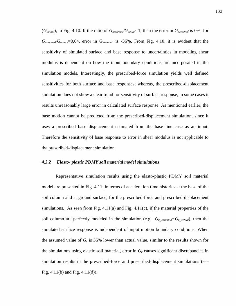
(Gactual), in Fig. 4.10. If the ratio of Gassumed/Gactual=1, then the error in Gassumed is 0%; for
Gassumed/Gactual=0.64, error in Gassumed is -36%. From Fig. 4.10, it is evident that the
sensitivity of simulated surface and base response to uncertainties in modeling shear
modulus is dependent on how the input boundary conditions are incorporated in the
simulation models. Interestingly, the prescribed-force simulation yields well defined
sensitivities for both surface and base responses; whereas, the prescribed-displacement
simulation does not show a clear trend for sensitivity of surface response, in some cases it
results unreasonably large error in calculated surface response. As mentioned earlier, the
base motion cannot be predicted from the prescribed-displacement simulation, since it
uses a prescribed base displacement estimated from the base line case as an input.
Therefore the sensitivity of base response to error in shear modulus is not applicable to
the prescribed-displacement simulation.
4.3.2 Elasto- plastic PDMY soil material model simulations
Representative simulation results using the elasto-plastic PDMY soil material
model are presented in Fig. 4.11, in terms of acceleration time histories at the base of the
soil column and at ground surface, for the prescribed-force and prescribed-displacement
simulations. As seen from Fig. 4.11(a) and Fig. 4.11(c), if the material properties of the
soil column are perfectly modeled in the simulation (e.g. Gr_assumed=Gr_actual), then the
simulated surface response is independent of input motion boundary conditions. When
the assumed value of Gr is 36% lower than actual value, similar to the results shown for
the simulations using elastic soil material, error in Gr causes significant discrepancies in
simulation results in the prescribed-force and prescribed-displacement simulations (see
Fig. 4.11(b) and Fig. 4.11(d)).
132
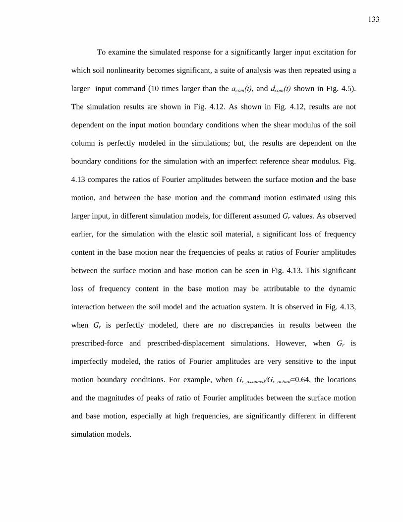
To examine the simulated response for a significantly larger input excitation for
which soil nonlinearity becomes significant, a suite of analysis was then repeated using a
larger input command (10 times larger than the acom(t), and dcom(t) shown in Fig. 4.5).
The simulation results are shown in Fig. 4.12. As shown in Fig. 4.12, results are not
dependent on the input motion boundary conditions when the shear modulus of the soil
column is perfectly modeled in the simulations; but, the results are dependent on the
boundary conditions for the simulation with an imperfect reference shear modulus. Fig.
4.13 compares the ratios of Fourier amplitudes between the surface motion and the base
motion, and between the base motion and the command motion estimated using this
larger input, in different simulation models, for different assumed Gr values. As observed
earlier, for the simulation with the elastic soil material, a significant loss of frequency
content in the base motion near the frequencies of peaks at ratios of Fourier amplitudes
between the surface motion and base motion can be seen in Fig. 4.13. This significant
loss of frequency content in the base motion may be attributable to the dynamic
interaction between the soil model and the actuation system. It is observed in Fig. 4.13,
when Gr is perfectly modeled, there are no discrepancies in results between the
prescribed-force and prescribed-displacement simulations. However, when Gr is
imperfectly modeled, the ratios of Fourier amplitudes are very sensitive to the input
motion boundary conditions. For example, when Gr_assumed/Gr_actual=0.64, the locations
and the magnitudes of peaks of ratio of Fourier amplitudes between the surface motion
and base motion, especially at high frequencies, are significantly different in different
simulation models.
133
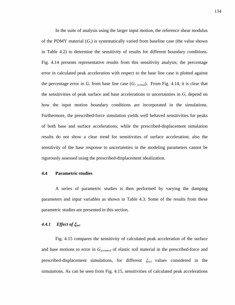
In the suite of analysis using the larger input motion, the reference shear modulus
of the PDMY material (Gr) is systematically varied from baseline case (the value shown
in Table 4.2) to determine the sensitivity of results for different boundary conditions.
Fig. 4.14 presents representative results from this sensitivity analysis; the percentage
error in calculated peak acceleration with respect to the base line case is plotted against
the percentage error in Gr from base line case (Gr_actual). From Fig. 4.14, it is clear that
the sensitivities of peak surface and base accelerations to uncertainties in Gr depend on
how the input motion boundary conditions are incorporated in the simulations.
Furthermore, the prescribed-force simulation yields well behaved sensitivities for peaks
of both base and surface accelerations; while the prescribed-displacement simulation
results do not show a clear trend for sensitivities of surface acceleration; also the
sensitivity of the base response to uncertainties in the modeling parameters cannot be
rigorously assessed using the prescribed-displacement idealization.
4.4 Parametric studies
A series of parametric studies is then performed by varying the damping
parameters and input variables as shown in Table 4.3. Some of the results from these
parametric studies are presented in this section.
4.4.1 Effect of ξact
Fig. 4.15 compares the sensitivity of calculated peak acceleration of the surface
and base motions to error in Gassumed of elastic soil material in the prescribed-force and
prescribed-displacement simulations, for different ξact values considered in the
simulations. As can be seen from Fig. 4.15, sensitivities of calculated peak accelerations
134
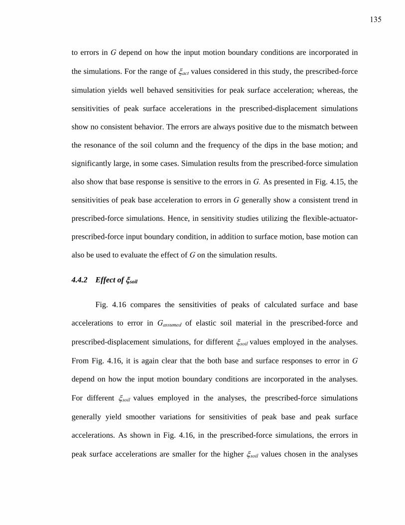
to errors in G depend on how the input motion boundary conditions are incorporated in
the simulations. For the range of ξact values considered in this study, the prescribed-force
simulation yields well behaved sensitivities for peak surface acceleration; whereas, the
sensitivities of peak surface accelerations in the prescribed-displacement simulations
show no consistent behavior. The errors are always positive due to the mismatch between
the resonance of the soil column and the frequency of the dips in the base motion; and
significantly large, in some cases. Simulation results from the prescribed-force simulation
also show that base response is sensitive to the errors in G. As presented in Fig. 4.15, the
sensitivities of peak base acceleration to errors in G generally show a consistent trend in
prescribed-force simulations. Hence, in sensitivity studies utilizing the flexible-actuator-
prescribed-force input boundary condition, in addition to surface motion, base motion can
also be used to evaluate the effect of G on the simulation results.
4.4.2 Effect of ξsoil
Fig. 4.16 compares the sensitivities of peaks of calculated surface and base
accelerations to error in Gassumed of elastic soil material in the prescribed-force and
prescribed-displacement simulations, for different ξsoil values employed in the analyses.
From Fig. 4.16, it is again clear that the both base and surface responses to error in G
depend on how the input motion boundary conditions are incorporated in the analyses.
For different ξsoil values employed in the analyses, the prescribed-force simulations
generally yield smoother variations for sensitivities of peak base and peak surface
accelerations. As shown in Fig. 4.16, in the prescribed-force simulations, the errors in
peak surface accelerations are smaller for the higher ξsoil values chosen in the analyses
135
and the errors in peak base accelerations are similar for both ξsoil=10% and ξsoil=25%;
however, they are different from the results shown for ξsoil=2.5%. For small soil damping
and the prescribed-displacement assumption, errors in G tend to result in greater peak
acceleration (due to energy being trapped in the soil specimen). In the prescribed-
displacement simulations, as soil damping increases, the sensitivity of peak surface
acceleration to errors in G decreases and shows consistent trends (see the prescribed-
displacement simulation results in Fig. 4.16 (b) and Fig. 4.16(c)). A higher soil damping
ratio may be deduced from the experiment if there are inconsistencies between the
resonant frequency (peaks in transfer function, see Fig. 4.9) and the dips in the base
motion (Elgamal et al. 2005). In some cases the sensitivity of peak surface acceleration to
errors in shear modulus was of opposite sign for the prescribed-force and prescribed-
displacement simulations.
4.4.3 Effect of actk & RMM
Representative results from a simulation of a linear soil model, with a relatively
stiff actuator ( 20/
=HGA
kact ) and a relatively heavy reaction mass ( 1.0=RM
soil
MM
), are
presented in Fig. 4.17; which may be compared to Fig. 4.7 and Fig. 4.8 for a more
flexible actuator and lighter reaction mass ( 1/
=HGA
kact , 5.0=RM
soil
MM ). Again we show
that if soil properties are perfectly modeled, the results are independent of the input
motion boundary conditions. If there is a 36% error in G, then the results do depend on
the input motion boundary condition. However if the actuator is relatively stiff and the
reaction mass is relatively heavy, the dependence on the input motion boundary condition
136
is relatively small. Hence, if a rigid actuator and heavy reaction mass are used in an
experiment, then it is reasonable to assume a prescribed-displacement input boundary
condition.
4.5 Ground motion analogy: Rigid and Compliant base
An example site response problem, illustrating how the sensitivities of predicted
surface response to uncertainties in modeling shear wave velocity of soil vary for
different input motion boundary conditions, was presented in Mejia et al. (2006). In their
study, a ‘deconvolution’ analysis using a 1-D wave propagation code, in this case a linear
analysis SHAKE, was performed to obtain an appropriate input at the base of a nonlinear
FLAC model. Seismic excitation to FLAC model was input using either a ‘rigid base’ or
a ‘compliant base’ options in FLAC. Details of these deconvolution procedures, and
different input motion boundary conditions are depicted in Fig. 4.18. As shown in Fig.
4.18, in both cases, the target earthquake, a modified recording from Kobe Earthquake,
was input at the top of the SHAKE column as an outcrop motion. Then, for the case
involving a ‘rigid base’ FLAC model, the motion at the top of the half space was
extracted as a ‘within’ motion and was applied as an acceleration time history to the base
of the FLAC model (shown in Fig. 4.18(a)). This excitation procedure is the same as the
prescribed-displacement input motion boundary condition described in this paper.
Whereas, for the case involving a ‘compliant base’ FLAC model, the upward propagating
wave motion (1/2 the outcrop motion) was extracted from SHAKE analysis at the top of
the half space and then used to convert the corresponding stress time history. Then the
estimated stress time history was applied to the base of the FLAC model (shown in Fig.
4.18(b)). This excitation procedure is analogous to the flexible-actuator-prescribed-force
137
input motion boundary condition described in this paper. When the soil properties are
perfectly modeled in the simulations, similar to the results shown in this paper, it was
shown in their study that the computed ground surface motions from FLAC models were
same for both ‘rigid base’ and ‘compliant base’ cases; and virtually identical to the target
motion, applied at ground surface as outcrop motion, used in SHAKE analysis.
Their study also addresses an interesting scenario to illustrate the relative
advantage of using the ‘compliant base’ idealization over the ‘rigid base’ idealization. In
this case, for simplicity, all layers were assigned a uniform shear wave velocity of 250
m/sec and uniform density. A SHAKE analysis was then performed to compute the
appropriate input for FLAC model. As explained earlier, the appropriate input for FLAC
model would be an acceleration time history of extracted ‘within’ motion for the ‘rigid
base’ case; and a stress time history, converted using the estimated upward propagating
wave motion for the ‘compliant base’ case. Then, the estimated inputs were adapted to
FLAC model that has a shear wave velocity 5% lower than the 250m/sec used in the
SHAKE analysis. Fig. 4.19 compares the calculated surface response from FLAC model
for both ‘rigid base’ and ‘compliant base’ cases. From Fig. 4.19, it is clear that the
sensitivity of ground surface response to a small error in shear wave velocity is very
sensitive to the input motion boundary conditions. Applying this mismatched input to
rigid-base as a prescribed displacement develops large amplitude periodic vibrations due
to the excitation of standing waves within the model (i.e. no energy transfer across the
“rigid-base” boundary). The mode shapes and the periods of vibration of these standing
waves can be seen, from the response spectrum, in Fig. 4.19(b). In contrast to the ‘rigid-
base’ case, the calculated ground surface motion in the ‘compliant-base’ case only
138
slightly differs from the target motion, and shows no presence of these standing waves
due to energy transfer across the “absorbing-base” boundary. Furthermore, it was argued
in their study that the presence of these reflections off the ‘rigid base’ is not always
readily apparent in complex non-linear FLAC analyses, as they can be masked by the
high damping at larger strains in non-linear soil models; and they can have a major
impact on analysis results, especially when cyclic degradation or liquefaction soil models
are employed. Hence a ‘compliant base’ is preferable to a ‘rigid base’, since it models
energy transfer out of the soil model through the base and accounts for the changes in the
motion at the base of the soil model caused by the errors in the frequencies of energy
absorption associated with the errors in input soil properties.
4.6 Discussion
4.6.1 Importance of proper treatment of boundary conditions on the sensitivity
analysis
In a validation phase of a computational simulation, it is common to perform in-
depth sensitivity studies to understand the sensitivity of simulation results to uncertainties
in modeling parameters. Arguably, sometimes, in these sensitivity studies less attention is
given to uncertainties in modeling boundary conditions. For example, in some cases,
numerical modelers make simplified assumptions in their simulations regarding the
complex boundary conditions involved in the actual problem (it could be an experiment
or a real physical problem) and use those simulations to perform sensitivity studies to
propagate the uncertainties in modeling parameters on the results. Results from these
sensitivity studies are then used validate the numerical simulations. But as we have
139

shown, the calculated sensitivities of the results are affected by the boundary conditions
used in the simulations. The conclusions drawn from sensitivity studies are not general if
sensitivities depend on the approximation of the boundary conditions.
4.6.2 Need for realistic numerical models of servo-hydraulic actuation system
Modeling the input motion boundary condition using the flexible-actuator-
prescribed-force approach requires a realistic representation of experimental boundary
conditions and the detailed modeling of various components of the centrifuge-shaker
system to include the effects of dynamic interaction between the test specimen and the
servo-hydraulic actuation system on the simulation results. In general, dynamic
interaction between a test specimen and the servo-hydraulic actuation system depends on
many factors such as characteristics of the test specimen, compliance of reaction mass,
compressibility of oil column in the actuator chamber, non-linear flow characteristics in
the actuator, servo valve time delay, configuration and characteristics of control loops,
etc. Therefore to fully incorporate the effects of the test specimen-actuation system
interaction on the simulation models, realistic models of actuator, servovalve, and
controller are required. Various analytical models to capture the salient features of
actuator, servovalve, and controller are available in the literature for structural shaking
table experiments and real-time pseudo dynamic testing in the context of structural
engineering (Conte et al. 2000, Williams et al. 2001, and Jung et al. 2006). It would be
ideal for a shaking table to have a heavy reaction mass and a stiff actuator so that the
effect of dynamic interaction between the soil model and actuation system on the test
results is minimal. Unfortunately, especially for most shaking tables on geotechnical
centrifuges, the real shaking tables are far from this ideal. Geotechnical centrifuge
140
experiments often involve relatively heavy and highly nonlinear test specimens (e.g., a
massive volume of liquefying sand). Additional work is required to understand the
interaction of highly nonlinear massive test specimens with non-ideal servo-hydraulic
actuation systems that are driven at their performance limits (in their nonlinear range).
4.7 Conclusions
Example simulations of a hypothetical centrifuge experiment have been presented
to illustrate the effects of using two different input motion boundary conditions on the
simulation results in various scenarios. In both the simulations using the linear elastic and
the elasto-plastic PDMY soil material models, if the shear modulus of the soil material is
perfectly modeled then the results are independent of the input motion boundary
conditions. Conversely, the predicted surface response is dependent on the input motion
boundary conditions when the shear modulus is imperfectly modeled in the simulations.
As expected, it is shown that the ratio of Fourier amplitudes between the surface motion
and the base motion (i.e surface transfer function) is also independent of the input motion
boundary conditions when a linear elastic soil material with an imperfect shear modulus
is employed in the analysis. However, the ratio of Fourier amplitude between the surface
motion and the base motion is dependent on the input motion boundary conditions when
a nonlinear soil material with an imperfect shear modulus is used in the analysis. In this
case, higher discrepancies are observed near frequencies at which peaks of ratio of
Fourier amplitudes occur. The ratio of Fourier amplitudes between the base motion and
the command motion (i.e. base transfer function) is dependent on the input motion
boundary conditions when the shear modulus of the soil material (both in linear elastic
and PDMY material) is imperfectly modeled in the simulations. This is because the dips
141
(valleys) in the base transfer function associated the energy absorption of the overlying
soil deposit occur at the natural periods of the soil, but the calculated amplification
(peaks) in the surface transfer function depends on the assumed natural periods which
depend on the assumed shear modulus in the simulations. If a prescribed-force input
motion boundary condition is assumed then the changes in frequency of dips correspond
to the changes in frequency of amplification. These changes in base response cannot be
evaluated using the prescribed-displacement input motion boundary condition.
Further, the flexible-actuator-prescribed-force approach which employs an
absorbing-base boundary generally yields well behaved sensitivities for results in a wide
range of simulation conditions. The prescribed-displacement approach, however, may
produce chaotic results. Therefore, when performing the numerical simulations on a
geotechnical centrifuge experiment, modeling input excitation using the first approach
may be preferable to the second approach.
The most general conclusion of this study is that the sensitivity of numerical
simulation results to uncertainties in modeling parameters depends on how the input
motion boundary conditions are accounted for and the dynamic interactions among the
various components of the dynamic system. This raises a fundamental question: How can
we assess the significance of a discrepancy between a numerical simulation and an
experimental result? A large error in response may be caused by a small error in input
parameter if, for example, a rigid boundary condition is assumed. . This paper shows that,
for shaking table tests, the significance of errors in the numerical simulations cannot be
rigorously assessed without accounting for dynamic interaction between the test
specimen and the actuation system.
142
4.8 Acknowledgements
The authors would like to acknowledge Prof. Ross Boulanger, Dr. Dan Wilson,
Lars Pedersen, and the staff of the UC Davis Center for Geotechnical Modeling for their
support in the course of this study. The operation and maintenance of the centrifuge
including development of a numerical model of the centrifuge shaker is made possible by
funding from NSF award # CMS-0402490 through a sub award from NEESinc.
4.9 References
Arulanandan, K,, and Scott, R. F., 1993. Project VELACS; control test results, Journal of
geotechnical engineering, 119(8), 1276-1292.
Conte, J. P., and Trombetti, T. L., 2000. Linear Dynamic Modeling of a Uni-Axial Servo-
Hydraulic Shaking Table System, Earthquake Engineering and Structural Dynamics,
Vol. 29, No. 9, pp. 1375-1404.
Elgamal, A., Yang, Z., Lai, T., Kutter, B.L., and Wilson, D.W., 2005. Dynamic Response
of Saturated Dense Sand in Laminated Centrifuge Container, J. Geotech. Geoenviron.
Eng., ASCE, 131(5) pp. 598-609.
Ilankatharan, M., and Kutter, B. L., 2008. Numerical Simulation of a Soil Model-Model
Container-Centrifuge Shaking Table System, Geotechnical Earthquake Engineering
and Soil Dynamics IV, D. Zeng, M. Manzari, and D. Hiltunen, eds., Geotechnical
Special Publication No. 181, ASCE, NY.
Jung, R. Y., and Shing, P. B., 2006. Performance evaluation of a real-time
pseudodynamic test system, Earthquake Engineering and Structural Dynamics, Vol.
35, No. 7, pp. 789-810.
143
Kutter, B.L., 1992. Dynamic centrifuge modeling of geotechnical structures,
Transportation Research Record 1336, TRB, National Research Council, National
Academy Press, Washington, D.C., pp. 24-30.
Kutter, B.L., 1995. Recent Advances in Centrifuge Modeling of Seismic Shaking, State-
of-the-Art Paper, Proceedings, Third International Conference on Recent Advances
in Geotechnical Earthquake Engineering and Soil Dynamics, St. Louis, MO, Vol.2,
pp. 927-942.
Mazzoni, S., McKenna, F., Scott, M.H., and Fenves, G., 2006. The OpenSees Command
Language Manual: version 1.7.3, Pacific Earthquake Engineering Center, Univ. of
Calif., Berkeley. ⟨http://opensees.berkeley.edu⟩.
Mejia, L.H., and Dawson, E.M., 2006. Earthquake Deconvolution for FLAC,
Proceedings, Fourth International FLAC Symposium on Numerical Modeling in
Geomechanics, Madrid, Spain.
Williams, D. M., Williams, M. S., and Blakeborough, A., 2001. Numerical Modeling of a
Servohydraulic Testing System for Structures, Journal of engineering mechanics,
127(8), 816-827.
Yang, Z., Elgamal, A., & Parra, E., 2003. Computational model for cyclic mobility and
associated shear deformation, Journal of geotechnical and geoenvironmental
engineering, 129(12), 1119-1127.
144
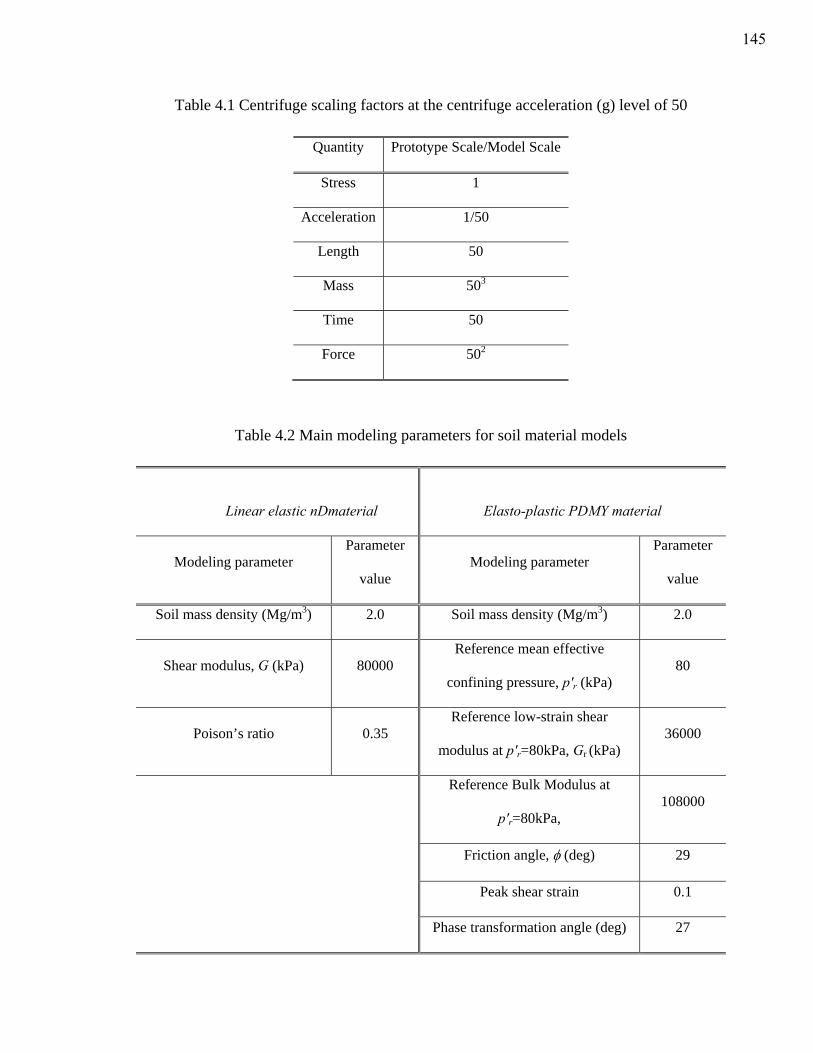
Table 4.1 Centrifuge scaling factors at the centrifuge acceleration (g) level of 50
Quantity Prototype Scale/Model Scale
Stress 1
Acceleration 1/50
Length 50
Mass 503
Time 50
Force 502
Table 4.2 Main modeling parameters for soil material models
Linear elastic nDmaterial
Elasto-plastic PDMY material
Modeling parameter Parameter
value Modeling parameter
Parameter
value
Soil mass density (Mg/m3) 2.0 Soil mass density (Mg/m3) 2.0
Shear modulus, G (kPa) 80000 Reference mean effective
confining pressure, p′r (kPa) 80
Poison’s ratio 0.35 Reference low-strain shear
modulus at p′r=80kPa, Gr (kPa) 36000
Reference Bulk Modulus at
p′r=80kPa, 108000
Friction angle, φ (deg) 29
Peak shear strain 0.1
Phase transformation angle (deg) 27
145
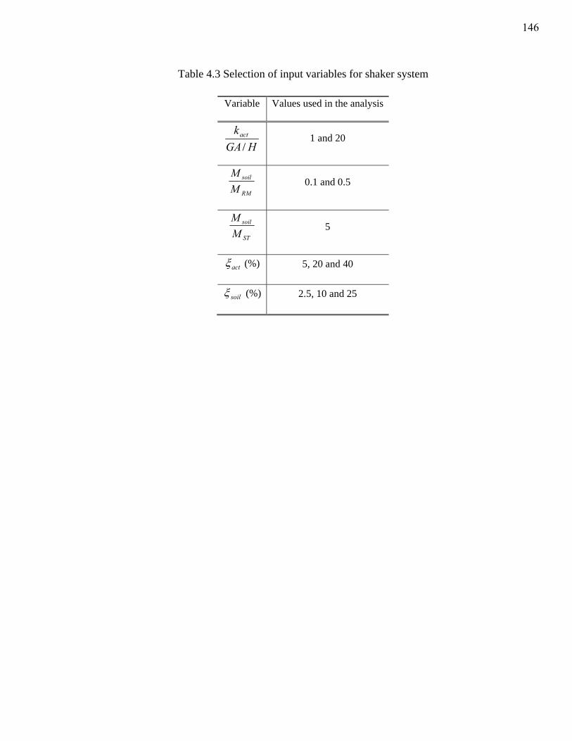
Table 4.3 Selection of input variables for shaker system
Variable Values used in the analysis
HGAkact
/ 1 and 20
RM
soil
MM
0.1 and 0.5
ST
soil
MM
5
actξ (%) 5, 20 and 40
soilξ (%) 2.5, 10 and 25
146
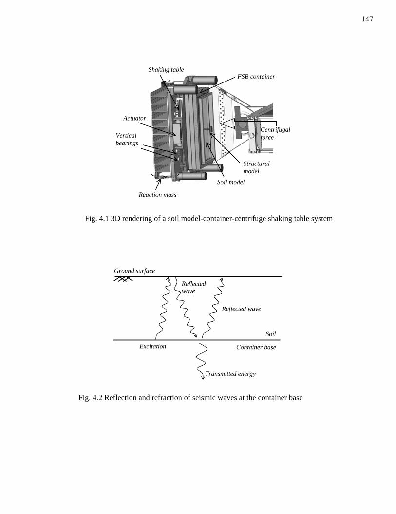
Fig. 4.1 3D rendering of a soil model-container-centrifuge shaking table system
Vertical bearings
FSB container
Soil model
Structural model
Centrifugal force
Actuator
Shaking table
Reaction mass
Fig. 4.2 Reflection and refraction of seismic waves at the container base
Reflected wave
Transmitted energy
Reflected wave
Soil
Container base Excitation
Ground surface
147
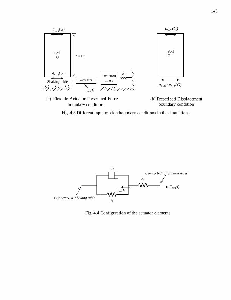
Fig. 4.4 Configuration of the actuator elements
Connected to reaction mass
k2
c2
Fcom(t)
Connected to shaking table
k1
Fcom(t)
Fig. 4.3 Different input motion boundary conditions in the simulations
(a) Flexible-Actuator-Prescribed-Force boundary condition
H=1m
Actuator
Soil G
aba(G)
as_pf(G)
Fcom(t)
Soil G
ab_pf(G)
Shaking table Actuator
kh Reaction mass
(b) Prescribed-Displacement boundary condition
Soil G
ab_pd=ab_pf(G)
as_pd(G)
148
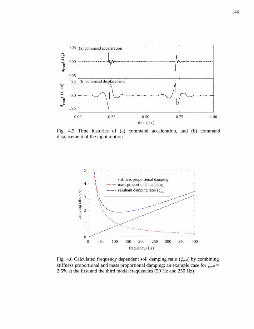
Fig. 4.5 Time histories of (a) command acceleration, and (b) command displacement of the input motion
(a) command acceleration
a com
(t) (g
)
-0.05
0.00
0.05
(b) command displacement
time (sec)0.00 0.25 0.50 0.75 1.00
d com
(t) (m
m)
-0.2
0.0
0.2
Fig. 4.6 Calculated frequency dependent soil damping ratio (ξsoil) by combining stiffness proportional and mass proportional damping: an example case for ξsoil = 2.5% at the first and the third modal frequencies (50 Hz and 250 Hz)
frequency (Hz)0 50 100 150 200 250 300 350 400
dam
ping
ratio
(%)
0
1
2
3
4
5
stiffness proportional dampingmass proportional dampingresultant damping ratio (ξsoil)
149
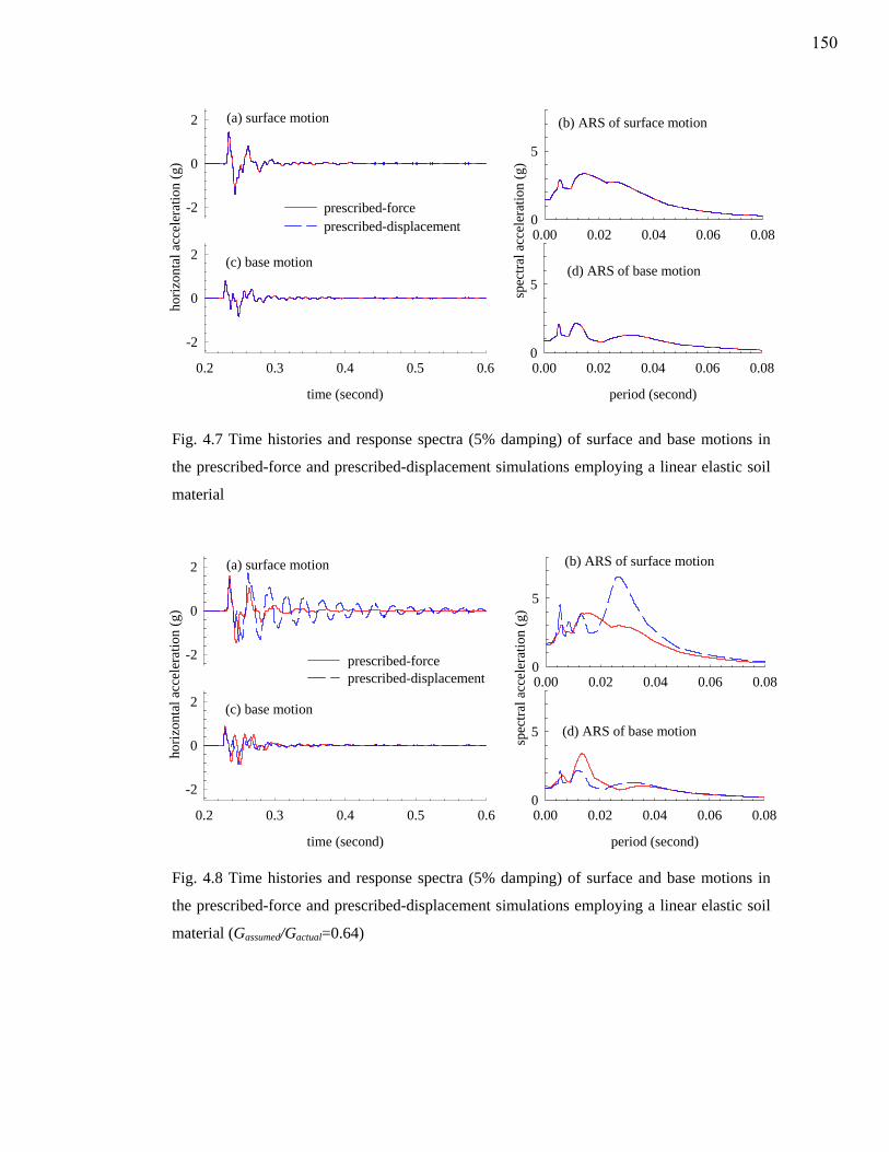
(c) base motion
time (second)
0.2 0.3 0.4 0.5 0.6
-2
0
2
(a) surface motion
horiz
onta
l acc
eler
atio
n (g
)
-2
0
2
prescribed-forceprescribed-displacement
(d) ARS of base motion
period (second)
0.00 0.02 0.04 0.06 0.080
5
(b) ARS of surface motion
0.00 0.02 0.04 0.06 0.08
spec
tral a
ccel
erat
ion
(g)
0
5
Fig. 4.8 Time histories and response spectra (5% damping) of surface and base motions in
the prescribed-force and prescribed-displacement simulations employing a linear elastic soil
material (Gassumed/Gactual=0.64)
Fig. 4.7 Time histories and response spectra (5% damping) of surface and base motions in
the prescribed-force and prescribed-displacement simulations employing a linear elastic soil
material
(c) base motion
time (second)
0.2 0.3 0.4 0.5 0.6
-2
0
2
(a) surface motion
horiz
onta
l acc
eler
atio
n (g
)
-2
0
2
prescribed-forceprescribed-displacement
(b) ARS of surface motion
0.00 0.02 0.04 0.06 0.08
spec
tral a
ccel
erat
ion
(g)
0
5
(d) ARS of base motion
period (second)
0.00 0.02 0.04 0.06 0.080
5
150
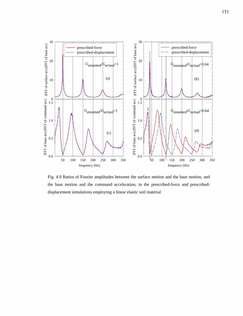
Gassumed/Gactual=1
|FFT
of s
urfa
ce a
cc| /|
FFT
of b
ase
acc|
0
10
20
30
prescribed-forceprescribed-displacement
Gassumed/Gactual=1
frequency (Hz)50 100 150 200 250 300 350
|FFT
of b
ase
acc| /
|FFT
of c
omm
and
acc|
0.0
0.5
1.0
1.5
Gassumed/Gactual=0.64
|FFT
of s
urfa
ce a
cc| /|
FFT
of b
ase
acc|
0
10
20
30
Gassumed/Gactual=0.64
frequency (Hz)50 100 150 200 250 300 350
|FFT
of b
ase
acc| /
|FFT
of c
omm
and
acc|
0.0
0.5
1.0
1.5
(a) (b)
(c) (d)
prescribed-forceprescribed-displacement
Fig. 4.9 Ratios of Fourier amplitudes between the surface motion and the base motion, and
the base motion and the command acceleration, in the prescribed-force and prescribed-
displacement simulations employing a linear elastic soil material
151
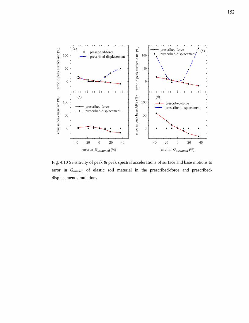
(a)
erro
r in
peak
surf
ace
acc
(%)
0
50
100prescribed-forceprescribed-displacement
(c)
error in Gassumed (%)
-40 -20 0 20 40
erro
r in
peak
bas
e ac
c (%
)
0
50
100
(b)
erro
r in
peak
surf
ace
AR
S (%
)
0
50
100
(d)
error in Gassumed (%)
-40 -20 0 20 40
erro
r in
peak
bas
e A
RS
(%)
0
50
100
prescribed-forceprescribed-displacement
prescribed-forceprescribed-displacement
prescribed-forceprescribed-displacement
Fig. 4.10 Sensitivity of peak & peak spectral accelerations of surface and base motions to
error in Gassumed of elastic soil material in the prescribed-force and prescribed-
displacement simulations
152
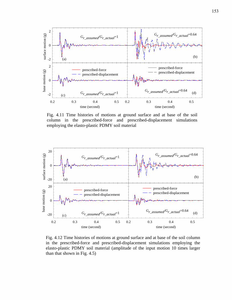
time (second)0.2 0.3 0.4 0.5
base
mot
ion
(g)
-2
0
2
Gr_assumed/Gr_actual=1
surf
ace
mot
ion
(g)
-2
0
2
-2
0
2
absorbing-baserigid-base
time (second)0.2 0.3 0.4 0.5
Gr_assumed/Gr_actual=1
Gr_assumed/Gr_actual=0.64
Gr_assumed/Gr_actual=0.64
(a) (b)
(c) (d)
absorbing-baserigid-base
prescribed-forceprescribed-displacement
prescribed-forceprescribed-displacement
Fig. 4.11 Time histories of motions at ground surface and at base of the soil column in the prescribed-force and prescribed-displacement simulations employing the elasto-plastic PDMY soil material
Fig. 4.12 Time histories of motions at ground surface and at base of the soil column in the prescribed-force and prescribed-displacement simulations employing the elasto-plastic PDMY soil material (amplitude of the input motion 10 times larger than that shown in Fig. 4.5)
time (second)0.2 0.3 0.4 0.5
base
mot
ion
(g)
-20
0
20
Gr_assumed/Gr_actual=1
surf
ace
mot
ion
(g)
-20
0
20
-20
0
20
absorbing-baserigid-base
time (second)0.2 0.3 0.4 0.5
Gr_assumed/Gr_actual=1
Gr_assumed/Gr_actual=0.64
Gr_assumed/Gr_actual=0.64
(a) (b)
(c) (d)
absorbing-baserigid-base
prescribed-forceprescribed-displacement
prescribed-forceprescribed-displacement
153
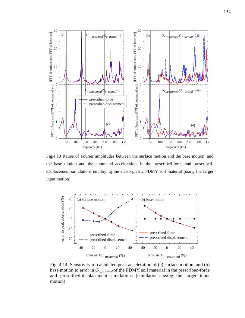
Gr_assumed/Gr_actual=1
frequency (Hz)50 100 150 200 250 300 350
|FFT
of b
ase
acc| /
|FFT
of c
omm
and
acc|
0
1
2
3
Gr_assumed/Gr_actual=1
|FFT
of s
urfa
ce a
cc| /|
FFT
of b
ase
acc|
0
10
20
30
prescribed-forceprescribed-displacement
Gr_assumed/Gr_actual=0.64
|FFT
of s
urfa
ce a
cc| /|
FFT
of b
ase
acc|
0
10
20
30
Gr_assumed/Gr_actual=0.64
frequency (Hz)50 100 150 200 250 300 350
|FFT
of b
ase
acc| /
|FFT
of c
omm
and
acc|
0
1
2
3
(a)
(c)
(b)
(d)
Fig.4.13 Ratios of Fourier amplitudes between the surface motion and the base motion, and
the base motion and the command acceleration, in the prescribed-force and prescribed-
displacement simulations employing the elasto-plastic PDMY soil material (using the larger
input motion)
Fig. 4.14. Sensitivity of calculated peak acceleration of (a) surface motion, and (b) base motion to error in Gr_assumed of the PDMY soil material in the prescribed-force and prescribed-displacement simulations (simulations using the larger input motion)
(b) base motion
error in Gr_assumed (%)
-40 -20 0 20 40
(a) surface motion
error in Gr_assumed (%)
-40 -20 0 20 40
erro
r in
peak
acc
eler
atio
n (%
)
-20
-10
0
10
20
absorbing-baserigid-base
absorbing-baserigid-base
prescribed-forceprescribed-displacement
prescribed-forceprescribed-displacement
154
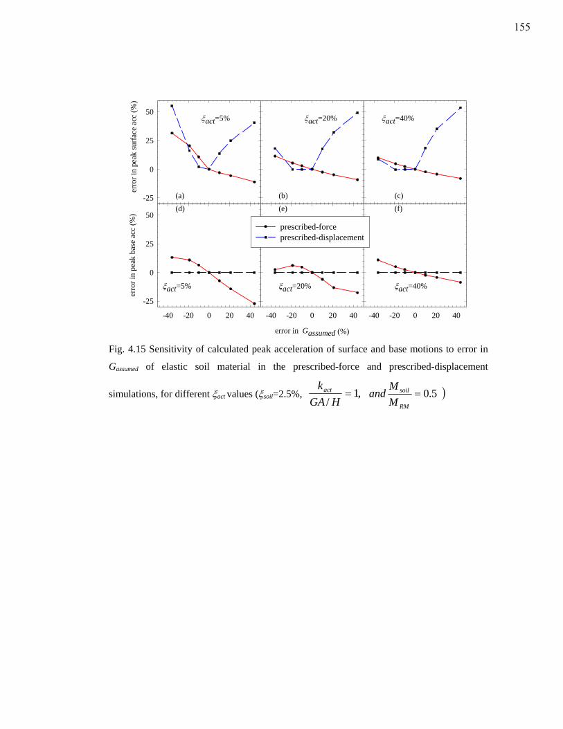
-40 -20 0 20 40
erro
r in
peak
bas
e ac
c (%
)
-25
0
25
50
erro
r in
peak
surf
ace
acc
(%)
-25
0
25
50
error in Gassumed (%)
-40 -20 0 20 40 -40 -20 0 20 40
prescribed-forceprescribed-displacement
ξact=20% ξact=40%ξact=5%
ξact=5% ξact=20% ξact=40%
(a) (b) (c)(d) (e) (f)
Fig. 4.15 Sensitivity of calculated peak acceleration of surface and base motions to error in
Gassumed of elastic soil material in the prescribed-force and prescribed-displacement
simulations, for different ξact values (ξsoil=2.5%, ,1/
=HGA
kact
)5.0=
RM
soil
MM
and
155
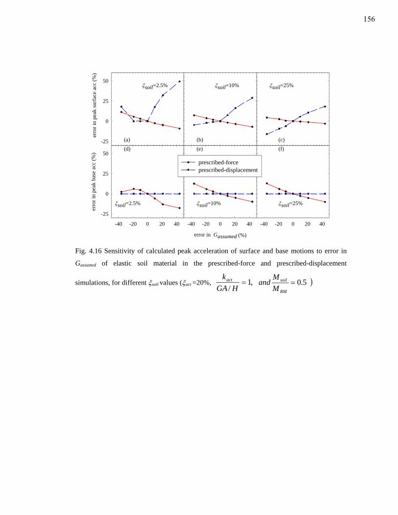
-40 -20 0 20 40
erro
r in
peak
bas
e ac
c (%
)
-25
0
25
50
erro
r in
peak
surf
ace
acc
(%)
-25
0
25
50
error in Gassumed (%)
-40 -20 0 20 40 -40 -20 0 20 40
prescribed-forceprescribed-displacement
ξsoil=10% ξsoil=25%ξsoil=2.5%
ξsoil=2.5% ξsoil=10% ξsoil=25%
(a) (b) (c)(d) (e) (f)
Fig. 4.16 Sensitivity of calculated peak acceleration of surface and base motions to error in
Gassumed of elastic soil material in the prescribed-force and prescribed-displacement
simulations, for different ξsoil values (ξact =20%, ,1/
=HGA
kact
)5.0=
RM
soil
MM
and
156
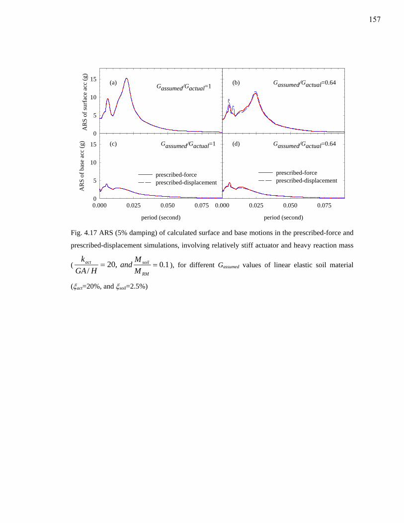
period (second)
0.000 0.025 0.050 0.075
period (second)
0.000 0.025 0.050 0.075
AR
S of
bas
e ac
c (g
)
0
5
10
15
AR
S of
surf
ace
acc
(g)
0
5
10
15
prescribed-forceprescribed-displacement
Gassumed/Gactual=1 Gassumed/Gactual=0.64
Gassumed/Gactual=1 Gassumed/Gactual=0.64
(a) (b)
(c) (d)
prescribed-forceprescribed-displacement
Fig. 4.17 ARS (5% damping) of calculated surface and base motions in the prescribed-force and
prescribed-displacement simulations, involving relatively stiff actuator and heavy reaction mass
( ,20/
=HGA
kact 1.0=RM
soil
MM
and ), for different Gassumed values of linear elastic soil material
(ξact=20%, and ξsoil=2.5%)
157
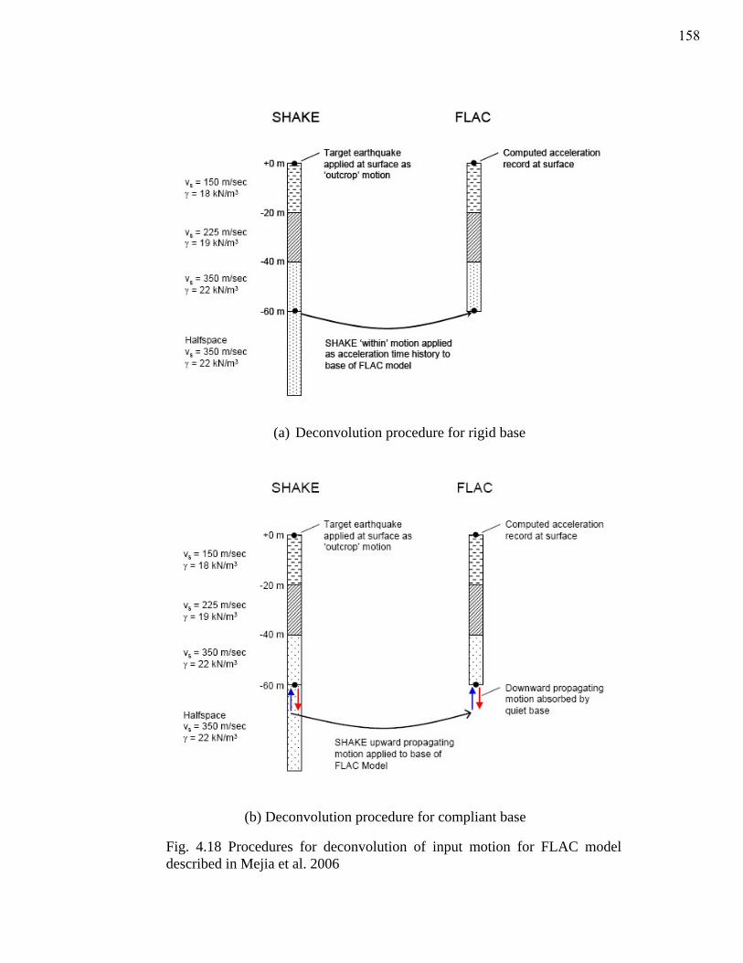
Fig. 4.18 Procedures for deconvolution of input motion for FLAC model described in Mejia et al. 2006
(a) Deconvolution procedure for rigid base
(b) Deconvolution procedure for compliant base
158
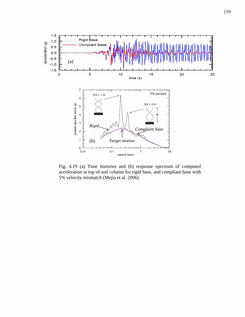
Fig. 4.19 (a) Time histories and (b) response spectrum of computed acceleration at top of soil column for rigid base, and compliant base with 5% velocity mismatch (Mejia et al. 2006)
(a)
Rigid Compliant base
Target motion (b)
159
Chapter 5
Numerical modeling of a soil-model container-centrifuge shaking table
system
This chapter presents a numerical model that was developed using OpenSees to
represent the dynamics of a soil-model container-centrifuge shaking table system. In the
numerical model, the soil, container, and shaking table were modeled using 2-D solid finite
elements. The mass and stiffness of the container as well as shear rods used to provide
complementary shear stress at the ends of the container were taken into account. The
actuator flexibility was included, and the excitation to the system was applied through the
actuator elements. Stiffness of the vertical bearing supports on the base of the container
and mass of the reaction mass were included in the analysis. The contents of this chapter
are extracted from a published paper and some additional details also included here for
completeness. The complete reference of the paper is given below.
Ilankatharan, M., and Kutter, B. L. (2008). “Numerical Simulation of a Soil Model-Model
Container-Centrifuge Shaking Table System.” Geotechnical Earthquake Engineering and
Soil Dynamics IV, D. Zeng, M. Manzari, and D. Hiltunen, eds., Geotechnical Special
Publication No. 181, ASCE, NY.
160
Abstract: A numerical model is developed using OpenSees to represent the dynamics of a
soil model-model container-centrifuge shaking table system. The centrifuge shaker-system
includes soil model, the flexible shear beam model container, shaking table and its reaction
mass. All of these different components interact with the soil model during dynamic
excitation, with some absorbing energy and others allowing undesired modes to affect the
response observed in the experiment. This interaction of soil model and
centrifuge/actuation system might attenuate or amplify the discrepancies in the responses
of the numerical and physical models. The relative error between a numerical simulation
and a physical simulation depends on how the boundary conditions and interaction among
different components in the physical model are included in the numerical model.
Assessment of the quality of a comparison between a numerical and physical simulation
should account for the effects of the boundary conditions and dynamic interaction among
different components in the dynamic system. This chapter outlines the details of the
simulation model, presents some representative results from simulations, discusses the
effect of interaction among different components on the responses, and presents how the
sensitivity of simulation outputs to uncertainties in the material properties depends on
boundary conditions in the physical and numerical simulations.
161
5.1 Introduction
One of the greatest challenges that earthquake engineers face is the paucity of data
available to evaluate the performance of geotechnical/structural systems during strong
earthquake motions. Earthquake engineers use laboratory experiments to understand the
performance of key components of foundation and structural systems under control
loading conditions. In this context, the use of dynamic centrifuge modeling has been
recognized by the researchers over the past 30 years. Dynamic centrifuge modeling of
geotechnical systems designed with varying soil profile characteristics,
substructure/superstructure characteristics, loading protocols, and detailed instrumentation
is used to obtain physical data, gain insight into the mechanisms involved, and perform
parametric studies to calibrate numerical models.
The Center for Geotechnical Modeling at University of California, Davis operates a
9.1m radius geotechnical centrifuge (a photograph shown in Fig 5.1) equipped with a 2 m x
1 m servo hydraulic shaking table to perform realistic earthquake simulations on the soil
models at prototype stress field conditions. Recent upgrades, funded by National Science
Foundation of United States through NEES (Network for Earthquake Engineering
Simulation), has increased the capacity of centrifuge and involved implementation of
advanced instrumentation (wireless data acquisition system, high speed video cameras,
etc), robotics, geophysical testing tools, and bi-axial shaking capability. These upgrades
increased the quantity as well as the quality of physical simulations (Wilson et al. 2007).
A 3D rendering of the UC Davis centrifuge-shaker system is shown in Fig. 5.2. The
centrifuge-shaker system includes a soil model, a flexible shear beam model container, a
shaking table and its reaction mass. All of these different components, with their own
162
resonant frequencies of vibration, interact with the soil model during dynamic excitation,
some absorbing energy, some allowing undesired modes to affect the response observed in
the experiment. This interaction of the soil model and the centrifuge/actuation system
might attenuate or amplify the discrepancies in responses of the numerical and physical
models. Qualitative assessment of issues of this interaction among soil model, container,
and shaker were addressed by many researchers in the past (Fiegel et al. 1994, Narayanan,
1999). However, a detailed numerical model to mathematically represent the dynamics of
the soil-model container-shaker system is necessary for comprehensive understanding of
this interaction and quantifying the effect of this interaction on the test results.
A 2D finite element model is developed using OpenSees (Open System for
Earthquake Engineering Simulation, http://opensees.berkeley.edu/index.php) to represent
the dynamics of centrifuge-shaking table-model container-soil model system. Data from
series of highly instrumented centrifuge tests that were performed as a part of NEES
collaboration project (Ilankatharan et al. 2005) and presented in the Chapter 2 of this
dissertation are used to validate the numerical procedure. The dimensions of the finite
element domain, all modeling parameters, and the results are presented in centrifuge model
scale (52g-increased gravity field) unless otherwise specified. The centrifuge scaling
factors for some physical properties was given in Table 4.1, further details on the
centrifuge scaling laws can be found in Kutter (1992).
5.2 Modeling system components
In the numerical model, the soil, container, and shaking table are modeled using
2-D solid finite elements. The following sections describe the details of numerical models
of these various system components.
163
5.2.1 Soil Model
Dry Nevada sand of a target relative density of 80% (with a thickness of 534mm) is
considered to represent the soil profile. The key soil properties of Nevada sand can be
found in centrifuge test series data report Ilankatharan et al. 2005. In OpenSees, soil is
modeled with four-node quad elements using PressureDependentMultiYield (PDMY),
elasto-plastic constitutive model (Yang et al, 2003). A complete description of material
model and recommended modeling parameters can be found at
http//cyclic.ucsd.edu/opensees/. Table 5.1 lists the main modeling parameters for this
dry-dense Nevada sand stratum. Within the PDMY material, the following equation
defines the low-strain shear modulus of soil (G) as a function of instantaneous effective
confinement (p’).
5.0
''⎟⎟⎠
⎞⎜⎜⎝
⎛=
rr p
pGG
The reference low-strain shear modulus (Gr) of Nevada sand is defined based on the
shear wave velocity data available in the literature for 80% relative density dry Nevada
sand (Arulnathan et al. 2000). In addition to the hysteric damping generated by the
stress-strain loops of PDMY material, very small amount of stiffness-proportional
damping is employed for the purpose of numerical stability with an average of 3% over the
frequency range of interest (1-500Hz). The estimated damping ratios at different
frequencies based on this employed stiffness-proportional damping are shown in Fig. 5.3.
164
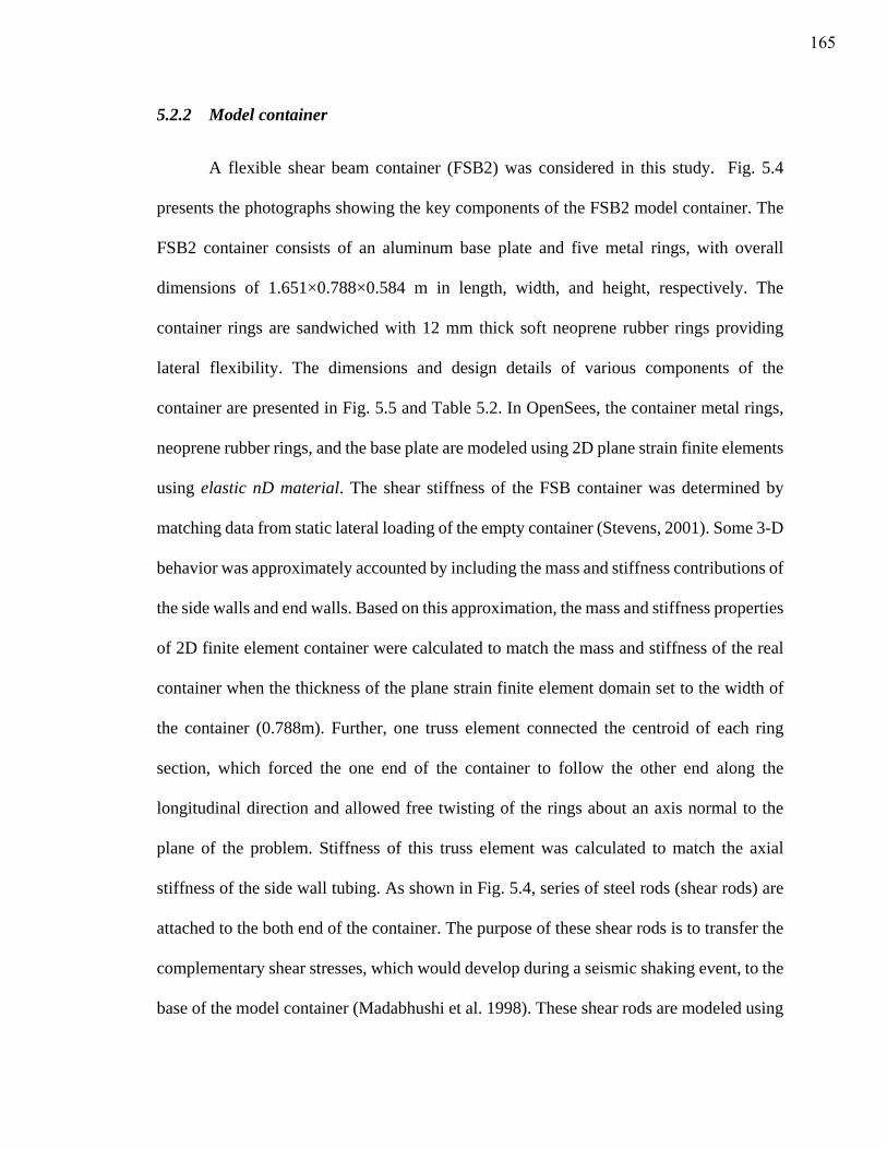
5.2.2 Model container
A flexible shear beam container (FSB2) was considered in this study. Fig. 5.4
presents the photographs showing the key components of the FSB2 model container. The
FSB2 container consists of an aluminum base plate and five metal rings, with overall
dimensions of 1.651×0.788×0.584 m in length, width, and height, respectively. The
container rings are sandwiched with 12 mm thick soft neoprene rubber rings providing
lateral flexibility. The dimensions and design details of various components of the
container are presented in Fig. 5.5 and Table 5.2. In OpenSees, the container metal rings,
neoprene rubber rings, and the base plate are modeled using 2D plane strain finite elements
using elastic nD material. The shear stiffness of the FSB container was determined by
matching data from static lateral loading of the empty container (Stevens, 2001). Some 3-D
behavior was approximately accounted by including the mass and stiffness contributions of
the side walls and end walls. Based on this approximation, the mass and stiffness properties
of 2D finite element container were calculated to match the mass and stiffness of the real
container when the thickness of the plane strain finite element domain set to the width of
the container (0.788m). Further, one truss element connected the centroid of each ring
section, which forced the one end of the container to follow the other end along the
longitudinal direction and allowed free twisting of the rings about an axis normal to the
plane of the problem. Stiffness of this truss element was calculated to match the axial
stiffness of the side wall tubing. As shown in Fig. 5.4, series of steel rods (shear rods) are
attached to the both end of the container. The purpose of these shear rods is to transfer the
complementary shear stresses, which would develop during a seismic shaking event, to the
base of the model container (Madabhushi et al. 1998). These shear rods are modeled using
165
elastic beam column elements in the OpenSees numerical model. At the both ends of the
container, soil nodes are slaved with shear rod nodes in both horizontal and vertical
directions. The vertical bearing supports at the base of the container (shown in Fig. 5.6) are
included to incorporate the possibility of rocking of the container; the stiffness of these
bearings is modeled using elastic zero-length elements. Torsional stiffness and bending of
the rings and friction on the sides of the container were not accounted for; these were
considered to have a secondary effect on the conclusions of this study.
5.2.3 Shaker and Reaction mass
The horizontal shaking table system of the UC Davis centrifuge facility is
considered for this present study. The plan view of this shaking table system is shown in
Fig. 5.6. The horizontal shaker is driven by two servo-hydraulic actuators, which are
visible in above Figure. The design detail and actuator mechanism of the horizontal
actuation system is described in Kutter et al. (1994). The 2D finite element mesh of the
soil-model container-shaker system is depicted in Fig. 5.7. Zero-length elements, to
represent stiffness of the vertical bearing supports, connect the container base and the
reaction mass. The reaction mass is modeled using an elastic nD material, the mass of the
reaction mass is assumed to be two times the payload mass (mass of container and soil).
Excitation to the system is applied through the actuator elements. A simplified model of
actuator system, illustrated in Fig 5.8, was used for the analysis. The main components of
this actuator model are briefly described below.
1k - A stiff spring across which the input excitation is applied – this represents the stiffness
of the servo-control system; for the data presented here, it was chosen k1 = 10 k2. ( 1k =
8764640 kN/m)
166
2k - A spring to represent stiffness of the actuator due to compressibility of oil and
mechanical connections between the actuator and the payload. Assuming that the
compressibility of the oil is the most flexible component. 2k can be calculated using
following equation.
LAk β42 =
where, β is the bulk modulus of oil (105 psi); A is the cross sectional area of piston
( 2
4DA π
= , D=4inches); L is the stroke of piston (L=0.5 inches for average piston
position); and the multiplier four is to account for four pistons-two pistons per actuator
(the calculated 2k is then reduced by 50% to account for the reduction in stiffness due
to the volume of trapped oil and mechanical connections).
−2c A dashpot representing the damping associated with the actuator spring, k2. 2c is
calculated as follows.
critcc ξ=2
mkccrit 22=
where, ξ is the damping ratio (ξ =40%, assumed), critc is the critical damping, and
m is the payload mass (i.e., mass of the container and soil).
inputF - Excitation force command to the system. inputF is calculated as follows.
dkFinput 1=
where, d is the command displacement.
167
5.3 Boundary conditions in simulation models
To improve understanding of interactions among soil model, container, and shaker
system and to evaluate how the sensitivity of simulation results depends on boundary
conditions in experiment and simulation, the boundary conditions were treated with three
different levels of detail as described below (and depicted in Fig. 5.9).
5.3.1 1-D shear beam simulations of soil
In this suite of analyses, the container and actuator were excluded; a 1D shear-beam
type FE model is employed to simulate soil site response (Fig. 5.9(a)). The unit weight of
soil is increased by 30% to account for the effect of container mass (which is 30% of the
soil mass) on the inertia forces. Dynamic excitation, equal to the measured acceleration
time history at the base of the container, is applied to the bottom soil nodes as prescribed
displacements.
5.3.2 2-D simulations of soil and container
The FSB2 container is included in this simulation model. The mass and stiffness of
the container, and the vertical bearing supports at the base of the container are taken into
account. Dynamic excitation is imparted to the bottom container nodes along horizontal
direction (Fig. 5.9(b)). Measured acceleration time history at the base of the container is
used as prescribed displacements.
5.3.3 2-D simulations of soil, container, and shaker
The effect of the shaker is included, the flexibility of actuator and the mass of the
reaction mass are modeled as indicated in detail in Fig. 5.7 and schematically in Fig. 5.9(c).
168

In this series of simulations, the base of the container is treated as an absorbing boundary
so that the energy transfer out of the soil model through the shaking table and reaction mass
can be accounted; excitation to the system is applied as a force time history through the
actuator elements (Fig. 5.8) so that the motion at the container base can be calculated.
To begin the analysis, the command displacement (d) is calculated by double
integration of the acceleration time history measured at the base of the container in the
experiment. Fig 5.10 shows the time histories of, the measured acceleration at the base of
the container and the calculated command displacement for a frequency sweep input. The
base acceleration predicted from the simulation is then compared with measured base
acceleration in the experiment. A transfer function is calculated between the measured and
the predicted responses. This transfer function is then used to modify the initial command
displacement, to obtain a reasonable (but still not identical) agreement between the base
motion calculated and the input base motions for other two cases (1-D shear beam
simulations of soil and 2-D simulations of soil and container). Further details on this
process of modifying command displacement is described later in this chapter.
5.4 Simulation results
5.4.1 Soil horizontal accelerations from 1-D shear beam simulations of soil and 2-D
simulations of soil and container
Representative simulation results of a frequency sweep excitation from the 1-D soil
shear beam simulations and 2-D simulations of soil and container are shown in Fig. 5.11
and Fig. 5.12, in terms of acceleration time histories and the corresponding response
spectra (5% damping) along the soil profile. The computed accelerations close to base of
169
the container (100mm from bottom of the container) in both simulations are in reasonable
agreement with experiment. However, there are significant differences in simulation
results at other two locations. For instance, the peak in the response spectra at a period of
0.009 sec in the 1-D shear beam simulations of soil disappears when the container is
included. Also, the gradually decaying periodic vibration cycles present in the time
histories of acceleration (after 0.6 sec) predicted in the shear beam simulations are not
visible in the 2-D simulations of soil and container.
Fig. 5.13 and Fig. 5.14 compare the soil horizontal accelerations calculated in
above two simulation models for an input motion obtained from an earthquake recording
from the 1994 Northridge earthquake. Details of this Northridge input motion can be found
in Ilankatharan et al. 2005. As shown in the above figures soil accelerations predicted in
two simulation models show significant discrepancies (except near the base of the
container). Peaks shown in the response spectra at a period of 0.0095 sec in the 1-D shear
beam simulations of soil diminish when the container is included. Further, peak shown in
the response spectra, at a period of 0.0045 sec in the experiment, is better captured in the
2-D simulations of soil and container. The above results show the effects of dynamic
interaction between the soil model and model container on the soil site response. It can be
seen from above figures that, the inclusion of the model container in the simulation
improves the quality of the comparison between the simulation and the experiment.
5.4.2 Soil Vertical accelerations from 2-D simulations of soil and container
Fig. 5.15 compares the time histories and response spectra (5% damping) of soil
vertical accelerations computed in the 2-D simulations of soil and container at 50mm
below the ground surface at both ends of the container. The time histories of accelerations
170
in the experiment are 180 out of phase, show rocking response of the container. It can be
seen in the time histories of the computed accelerations, the rocking behavior of the
container is well captured when the compliance of the vertical bearing supports at the base
of the container is included in the analysis.
To understand the effect of shear rods on the vertical accelerations, the above
analysis was repeated without shear rods. In this case, the elastic beam column elements
which were used to model shear rods were excluded and at both ends of the container, soil
nodes were slaved with container nodes in both horizontal and vertical directions. Fig. 5.16
compares the vertical accelerations computed with and without shear rods. As expected,
the computed vertical accelerations without shear rods are larger than that of calculated
with shear rods. The shear rods in the simulations transfer the complementary shear
stresses, which would developed during dynamic shaking, to the base of the model
container and decrease the vertical accelerations which would caused by the unequal
vertical stress distribution.
5.4.3 Results from the 2-D simulations of soil, container, and shaker
Representative simulation results from the 2-D simulations of soil, container, and
shaker are presented in Fig. 5.17, in terms of acceleration time histories and response
spectra (5% damping) along the soil profile. As mentioned earlier, in this series of
simulations excitation to the system is applied as a force time history through the actuator
elements so that the motion at the base of the container can be calculated. Fig. 5.18
compares the calculated base motion with the measured base motion from the experiment.
From Fig. 5.18, the low frequency (higher period) components of the base motions are in
reasonable agreement; however, the base response shows discrepancies in other frequency
171
ranges. These discrepancies in calculated base response propagate along the soil profile;
hence, the computed soil accelerations significantly deviate from the measured
accelerations (see Fig. 5.17).
To provide an acceptable correspondence between the computed base motion and
the measured base motion, the initial command displacement is then modified using a
transfer function calculated between the measured and the computed base motion. Fig.
5.19 presents the computed base response using the modified command displacement. As
shown in Fig. 5.19, results are in reasonable (but not identical) agreement with the
experiment. Fig. 5.20 compares the computed site response using the modified command
displacement with the experimental results. The presented simplified shaker model (Fig.
5.8), with the modified command displacement, allows a reasonable prediction of the soil
site response.
Fig. 5.21 presents the transfer function which was used to modify the original
command displacement. As described before, the original command displacement was
obtained by double integration of measured acceleration time history at the base of the
container in the experiment (shown in Fig. 5.10). Therefore, when creating Fig. 5.21, the
command acceleration was same as the measured base acceleration. Transfer function
between the surface and base motions calculated in the simulations using the original
command displacement is shown in Fig. 5.22. It can be seen from the above figures, the
valleys in the transfer function between the calculated base motion and command motion
occur at the frequencies of the peaks in the transfer function between the calculated surface
and base motions, especially around 90Hz and 224Hz which are the natural frequencies of
the soil model. The soil model acts as a vibration absorber near its natural frequency, which
172
causes a significant amount of dynamic interaction between the soil model and the
actuation system.
Fig. 5.23 compares the transfer function the between the calculated and measured
base motions for different characteristics of input. As shown in Fig. 5.23, the transfer
functions for different inputs are identical in the low frequency range (up to 60Hz) and
nearly same in the frequency range of 80Hz to 200Hz; however, they are different in the
frequency range of 60Hz to 80Hz and in the high frequency range (after 200Hz).
Therefore, when using different seismic excitations in the simulations, it would require
different transfer functions to modify the original command displacements to get
reasonable prediction of the base motions.
The shaker model presented in this chapter (Fig. 5. 10) was extended to employ the
actuator command displacement, which was specified to the servo controller during the
experiment, to calculate the force input in the simulations. Details of these simulations and
the implications of results on the base motion prediction are presented in chapter 6 of this
dissertation.
5.5 Sensitivity Analysis
The reference shear modulus of the PDMY material is systematically varied from
baseline case (the value shown in Table 1) to determine the sensitivity of simulation results
for different boundary conditions. Fig 5.24 and Fig 5.25 compare the effect of varying
shear modulus on the calculated ground surface and base response spectrum for different
boundary conditions. Fig 5.26 presents the percentage change in ground surface response
(in terms of peak and peak spectral accelerations), with respect to the base line case, against
the percentage change in reference shear modulus (Gr) from base line case (Grbaseline). A
173
similar plot for base response is presented in Fig 5.27. From figures 5.24 and 5.26, it is
evident that the sensitivity of ground surface response depends on how the experimental
boundary conditions are incorporated in the simulation models. Interestingly, for this
example, the calculated ground surface response is almost insensitive to the shear modulus
when the boundary conditions are more realistically modeled in the simulation (see Fig.
5.24 (c)). However, in some cases, calculated ground surface responses from the 1-D shear
beam simulations of soil and the 2-D simulations of soil and container are very much
sensitive to the shear modulus used in the analysis. For instance, a 25% negative change in
Gr yields, a 95% increase in peak acceleration in the 1-D shear beam simulation of soil, a
73% increase in 2-D simulation of soil and container, and a 8% increase in the 2-D
simulation of soil, container and shaker (see Fig. 5.26 (a)). As shown in Fig 5.23 and Fig
5.25, base response is sensitive to the shear modulus used in the 2-D simulations of soil,
container, and shaker simulations. The other two simulation models use prescribed base
displacement (measured motion at the base of the container in the experiment) as an input;
therefore, the sensitivities of base responses to changes in shear modulus are not applicable
to these simulation models.
Fig. 5.28 and Fig. 5.29 present the sensitivity analysis results using different
earthquake motion. The earthquake motion used here is a frequency sweep, composed of
sinusoidal cycles with gradually decreasing frequencies (the frequency sweep used in the
previous simulations composed of sinusoidal cycles of gradually increasing frequencies
(see Fig. 5.10) ), with a peak base acceleration of 13g (measured at the container base). The
percentage changes in surface and base responses are shown against the percentage
changes shear modulus, in Fig. 5.28 and Fig. 5.29. It is again clear that the results are
174
dependent on how the boundary conditions are incorporated in the simulations. Further,
sensitivities of results predicted from the 2-D simulations of soil, container, and shaker
show consistent behaviors; whereas, the results from other two simulations do not show
consistent trends.
Similar to the findings presented in chapter 4, it is again observed that, the 2-D
simulations of soil, container, and shaker, which employ the
flexible-actuator-prescribed-force boundary condition to specify the seismic input,
generally yield well behaved sensitivities for results in different simulation conditions;
however, the other two simulation models, which use the prescribed-displacement
boundary condition to adapt the seismic input, may produce chaotic results for
sensitivities.
5.6 Archives of numerical models of a soil-container-shaker system
The OpenSees numerical models of the soil-container-shaker system are archived
in NEEScentral (http://central.nees.org). These simulation archives are categorized into 3
different simulation folders as follows (based on complexities in the boundary conditions):
Simulation of MIL 03_ 2D Soil Shear beam (described in section 5.3.1)
Simulation of MIL 03_2D Soil and FSB2 container (described in section 5.3.2)
Simulation of MIL 03_2D Soil, FSB2 container, and Shaker (described in section
5.3.3)
The simulation archives are publically available in NEEScentral for others to use.
As described earlier, the simulations of the soil-container-shaker system consider a
uniform dry-dense sand soil model, a flexible shear beam, and the horizontal shaker of the
175

UC Davis centrifuge facility. These numerical models could be modified to accommodate
different soil models. To do this, a user may follow the following guidelines;
a) Modify the geometry of the FE mesh and the definition of constitutive
models and input parameters of the soil model according to the soil model
used in a new experiment.
b) Update the FE mesh (i.e., node and element numbers) of the model
container and the shaker based on the new soil mesh (OpenSees
post-processor available on the OpenSees website may be used to visualize
the nodes).
c) Follow the modeling details of different components of the container
(container rings, shear rods, etc) and the shaker described in sections 5.2.2
and 5.2.3 of this chapter (some of these details are provided on the input
files of the archived simulations)
d) Define the input motion boundary condition (i.e., location and time history
of input excitation) as the procedures described in sections 5.3.3 and 5.4.3
of this chapter.
5.7 Summary
Modeling of complex dynamics interaction of a soil-model
container-centrifuge-shaker system is presented in this chapter. This modeling
incorporates mass and flexibility of the container, the effect of shear rods at both ends of
the container, stiffness of the vertical bearing supports at the base of the container,
flexibility of the actuator, and the effect of reaction mass. A simplistic approximation of
the actuator and control system using springs and dashpots is used to include first-order
176
effects of actuator flexibility on the interaction between the specimen and the shaking
table. As opposed to the 1-D shear beam simulations of soil, inclusion of the container in
the simulations results in more accurate simulation of the experiment. In addition, the
rocking behavior of the container is well captured when the compliance of the vertical
bearing supports at the base of the container is included in the analysis.
Results from sensitivity studies show that the sensitivity of computational
simulation output to changes in input parameters depends on how boundary conditions are
modeled in the simulation; to provide an unbiased validation of a numerical model, it is
important evaluate the effects of boundary conditions on the sensitivity of simulation
results. Similar to the results presented in chapter 4 for the simulations with the
hypothetical centrifuge experiment, it is again clear that the sensitivity results of the
simulations heavily depend on the input motion boundary conditions. In the simulations,
converse to specifying input using the prescribed-displacement boundary condition, using
the flexible-actuator-prescribed-force boundary condition generally yield well behaved
sensitivities for simulation results.
A spin-off benefit of accurate modeling the centrifuge shaker system is the
prediction of base motions in the simulations. Further, this numerical model could be used
to predict base motions during input motion tuning exercises prior to the actual experiment.
However, the dynamic interaction between the soil model and the servo-hydraulic
actuation system significantly affect the accuracy of predicted base motion. In general,
dynamic interaction between the soil model and the servo-hydraulic actuation system
depends on numerous factors such as the characteristics of the soil model, compressibility
of oil column in the actuator, non-linear flow characteristics in the actuator, servo valve
177
time delay, configuration and characteristics of control loops etc. The simplified shaker
model presented in this chapter incorporates some of the above features and uses measured
motion in the container base (in the experiment) to develop input command displacement.
Application of this model was extended to accommodate the actual command
displacement specified to the servo controller (during the experiment) as the command
displacement in the shaker model so that the motion at the container base could be
calculated. Details of these extensions and the results from these analyses are presented in
chapter 6 of this dissertation.
5.8 References
Arulnathan, R., Boulanger, R. W., Kutter, B. L., and Sluis, W. K. (2000). “New tool for
shear wave velocity measurements in model tests.” Geotechnical testing journal,
23(4): 444-453.
Fiegel, G.L., M.Hudson, I.M. Idriss, B.L. Kutter, and X. Zeng, (1994) "Effect of Model
Containers on Dynamic Soil Response", Centrifuge 94, Leung, Lee and Tan (eds.),
Balkema, Rotterdam, pp. 145-150.
Ilankatharan, M., Sasaki, T., Shin, H., Kutter, B. L., Arduino, P., and Kramer, S. L., 2005.
“A demonstration of NEES system for studying soil-foundation-structure interaction”
Centrifuge data report for MIL01. Rep. No. UCD/CGMDR-05/05, Ctr. for Geotech.
Modeling , Dept. of Civ. and Envir. Engrg., UC Davis.
Kutter, B.L. (1992). "Dynamic centrifuge modeling of geotechnical structures."
Transportation Research Record 1336, TRB, National Research Council, National
Academy Press, Washington, D.C., pp. 24-30.
Kutter, B.L., Idriss, I.M., Kohnke, T., Lakeland, J., Li, X.S., Sluis, W., Zeng, X.,
178
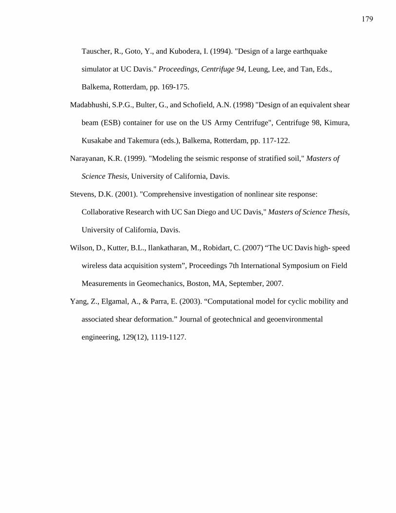
Tauscher, R., Goto, Y., and Kubodera, I. (1994). "Design of a large earthquake
simulator at UC Davis." Proceedings, Centrifuge 94, Leung, Lee, and Tan, Eds.,
Balkema, Rotterdam, pp. 169-175.
Madabhushi, S.P.G., Bulter, G., and Schofield, A.N. (1998) "Design of an equivalent shear
beam (ESB) container for use on the US Army Centrifuge", Centrifuge 98, Kimura,
Kusakabe and Takemura (eds.), Balkema, Rotterdam, pp. 117-122.
Narayanan, K.R. (1999). "Modeling the seismic response of stratified soil," Masters of
Science Thesis, University of California, Davis.
Stevens, D.K. (2001). "Comprehensive investigation of nonlinear site response:
Collaborative Research with UC San Diego and UC Davis," Masters of Science Thesis,
University of California, Davis.
Wilson, D., Kutter, B.L., Ilankatharan, M., Robidart, C. (2007) “The UC Davis high- speed
wireless data acquisition system”, Proceedings 7th International Symposium on Field
Measurements in Geomechanics, Boston, MA, September, 2007.
Yang, Z., Elgamal, A., & Parra, E. (2003). “Computational model for cyclic mobility and
associated shear deformation.” Journal of geotechnical and geoenvironmental
engineering, 129(12), 1119-1127.
179
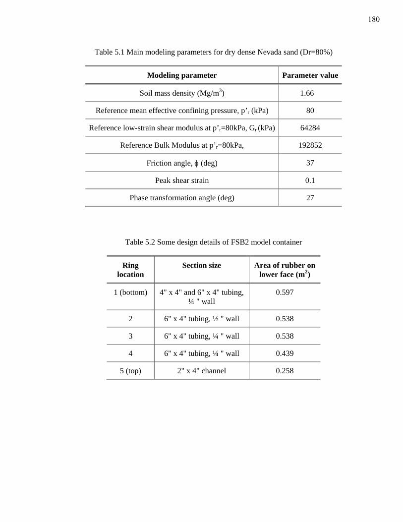
Table 5.1 Main modeling parameters for dry dense Nevada sand (Dr=80%)
Modeling parameter Parameter value
Soil mass density (Mg/m3) 1.66
Reference mean effective confining pressure, p’r (kPa) 80
Reference low-strain shear modulus at p’r=80kPa, Gr (kPa) 64284
Reference Bulk Modulus at p’r=80kPa, 192852
Friction angle, φ (deg) 37
Peak shear strain 0.1
Phase transformation angle (deg) 27
Table 5.2 Some design details of FSB2 model container
Ring location
Section size Area of rubber on lower face (m2)
1 (bottom) 4" x 4" and 6" x 4" tubing, ¼ " wall
0.597
2 6" x 4" tubing, ½ " wall 0.538
3 6" x 4" tubing, ¼ " wall 0.538
4 6" x 4" tubing, ¼ " wall 0.439
5 (top) 2" x 4" channel 0.258
180
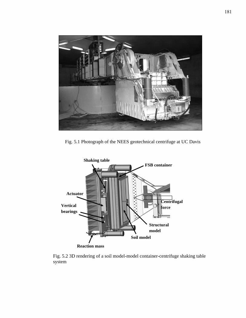
Fig. 5.1 Photograph of the NEES geotechnical centrifuge at UC Davis
Fig. 5.2 3D rendering of a soil model-model container-centrifuge shaking table system
Vertical bearings
FSB container
Soil model
Structural model
Centrifugal force
Actuator
Shaking table
Reaction mass
181
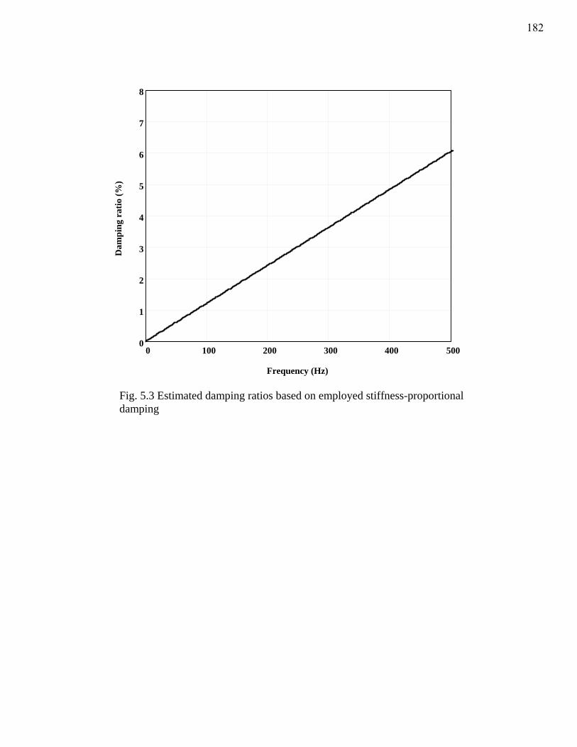
0 100 200 300 400 5000
1
2
3
4
5
6
7
8
Frequency (Hz)
Dam
ping
rat
io (%
)
Fig. 5.3 Estimated damping ratios based on employed stiffness-proportional damping
182
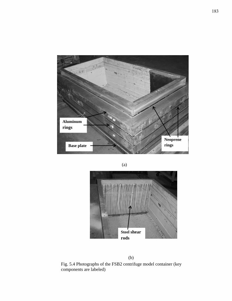
Aluminum rings
Neoprene rings Base plate
(a)
(b)
Steel shear rods
Fig. 5.4 Photographs of the FSB2 centrifuge model container (key components are labeled)
183
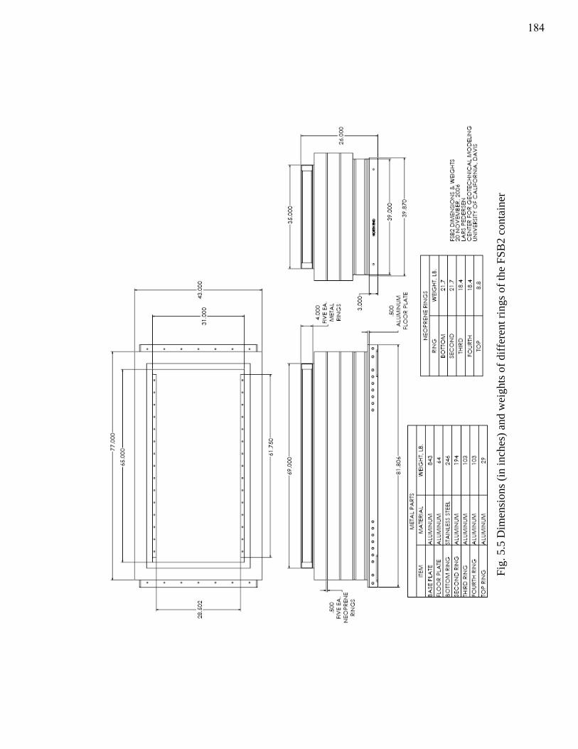
Fig.
5.5
Dim
ensi
ons (
in in
ches
) and
wei
ghts
of d
iffer
ent r
ings
of t
he F
SB2
cont
aine
r
184
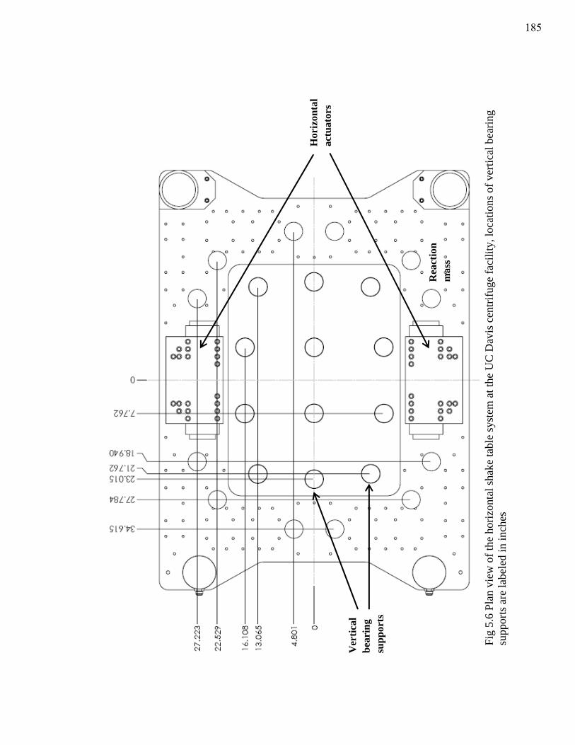
Fig
5.6
Plan
vie
w o
f the
hor
izon
tal s
hake
tabl
e sy
stem
at t
he U
C D
avis
cen
trifu
ge fa
cilit
y, lo
catio
ns o
f ver
tical
bea
ring
supp
orts
are
labe
led
in in
ches
Hor
izon
tal
actu
ator
s
Ver
tical
be
arin
g su
ppor
ts
Rea
ctio
n m
ass
185
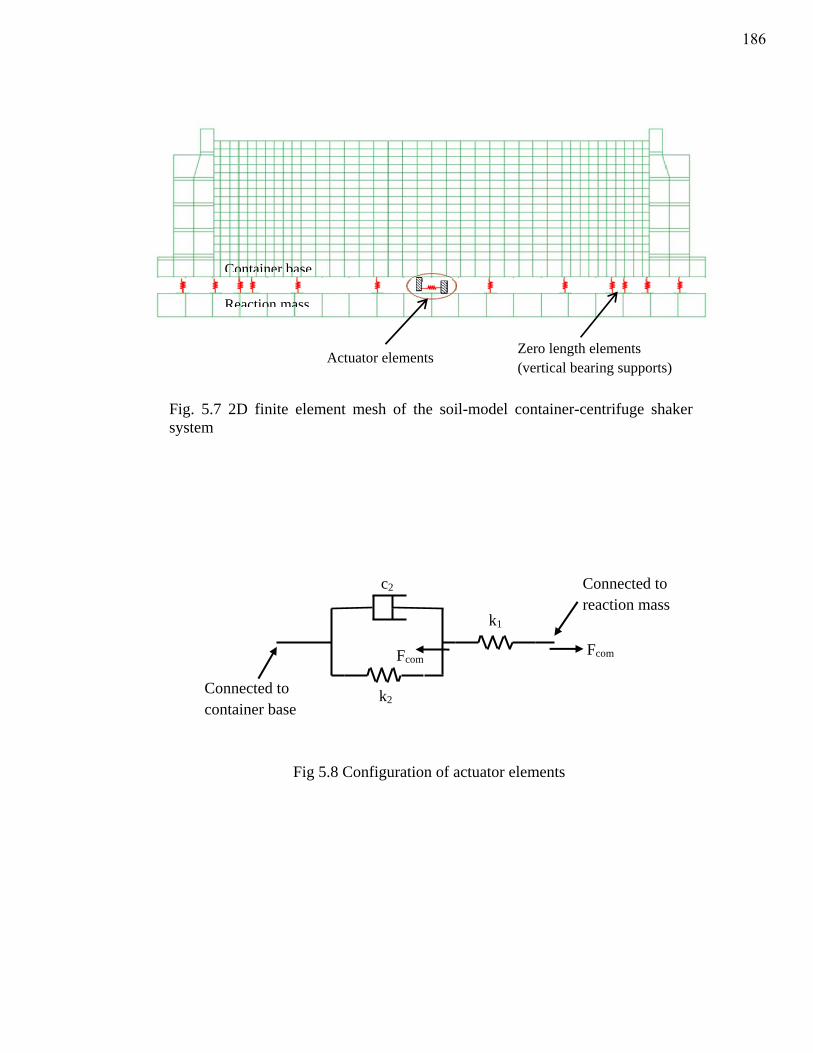
Fig 5.8 Configuration of actuator elements
Connected to reaction mass
k2
c2
Fcom
Connected to container base
k1
Fcom
Fig. 5.7 2D finite element mesh of the soil-model container-centrifuge shaker system
Container base
Reaction mass
Actuator elements Zero length elements (vertical bearing supports)
186
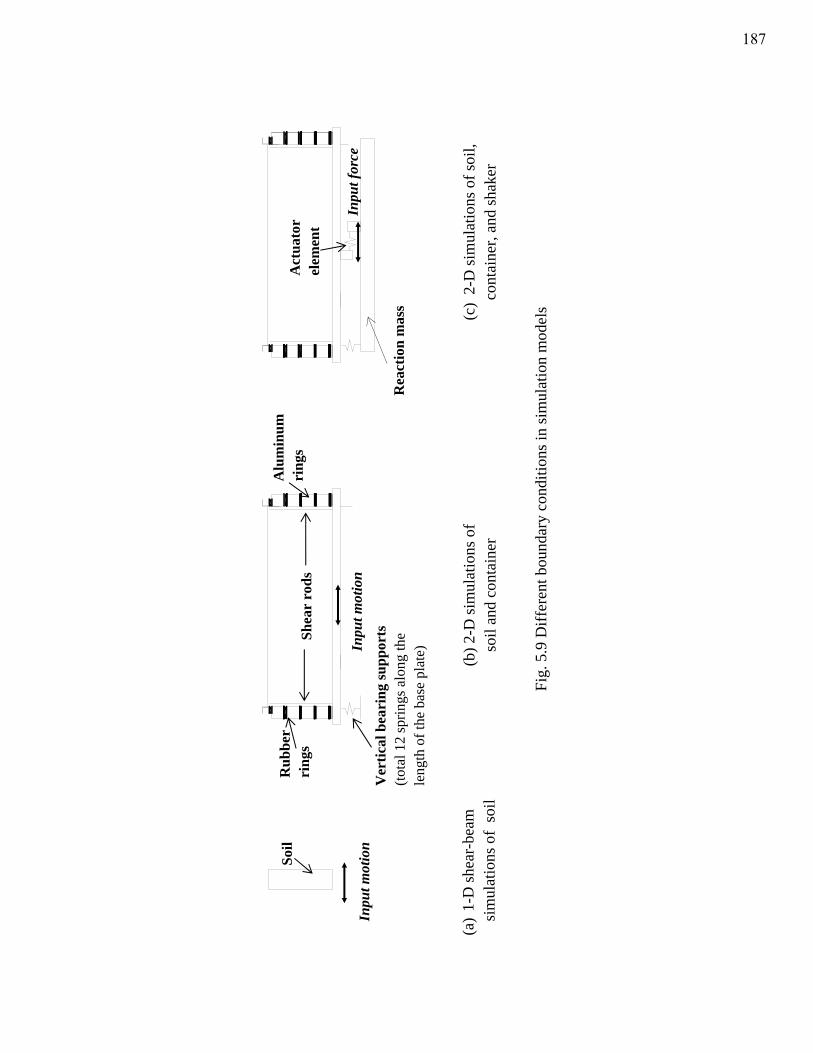
Fig.
5.9
Diff
eren
t bou
ndar
y co
nditi
ons i
n si
mul
atio
n m
odel
s
Act
uato
r el
emen
t
Inpu
t mot
ion
Inpu
t mot
ion
Rea
ctio
n m
ass
Inpu
t for
ce
Shea
r ro
ds
Alu
min
um
ring
s R
ubbe
r ri
ngs
Soil
Ver
tical
bea
ring
supp
orts
(to
tal 1
2 sp
rings
alo
ng th
e le
ngth
of t
he b
ase
plat
e)
(a)
1-D
shea
r-be
am
sim
ulat
ions
of
soil
(b) 2
-D si
mul
atio
ns o
f
soil
and
cont
aine
r (c
) 2-
D si
mul
atio
ns o
f soi
l, co
ntai
ner,
and
shak
er
187
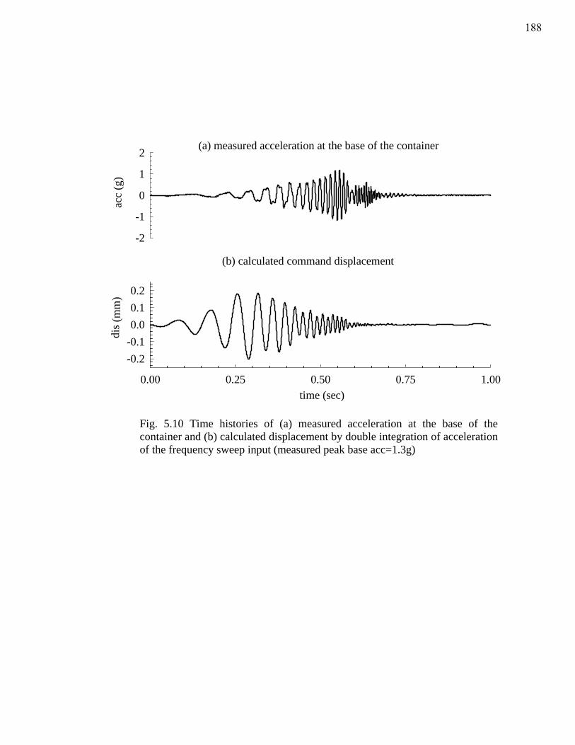
(a) measured acceleration at the base of the container
acc
(g)
-2
-1
0
1
2
(b) calculated command displacement
time (sec)0.00 0.25 0.50 0.75 1.00
dis (
mm
)
-0.2-0.10.00.10.2
Fig. 5.10 Time histories of (a) measured acceleration at the base of the container and (b) calculated displacement by double integration of acceleration of the frequency sweep input (measured peak base acc=1.3g)
188
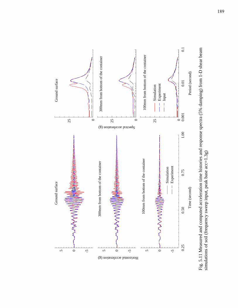
300m
m fr
om b
otto
m o
f the
con
tain
er
Horizontal acceleration (g)
-505
100m
m fr
om b
otto
m o
f the
con
tain
er
Tim
e (s
econ
d)
0.25
0.50
0.75
1.00
-505
Gro
und
surf
ace
-505
Sim
ulat
ion
Expe
rimen
t
Gro
und
surf
ace
025
100m
m fr
om b
otto
m o
f the
con
tain
er
Perio
d (s
econ
d)
0.00
10.
010.
1025
300m
m fr
om b
otto
m o
f the
con
tain
er
Spectral acceleration (g)
025
Sim
ulat
ion
Expe
rimen
tIn
put
Fig.
5.1
1 M
easu
red
and
com
pute
d ac
cele
ratio
n tim
e hi
stor
ies a
nd re
spon
se sp
ectra
(5%
dam
ping
) fro
m 1
-D sh
ear b
eam
si
mul
atio
ns o
f soi
l (fr
eque
ncy
swee
p in
put,
peak
bas
e ac
c=1.
3g)
189
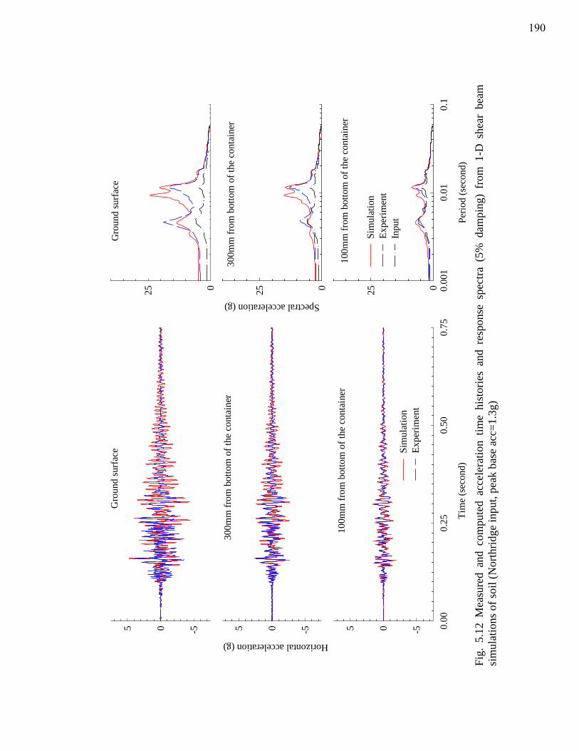
300m
m fr
om b
otto
m o
f the
con
tain
er
Horizontal acceleration (g)
-505
100m
m fr
om b
otto
m o
f the
con
tain
er
Tim
e (s
econ
d)
0.00
0.25
0.50
0.75
-505
Gro
und
surf
ace
-505
Sim
ulat
ion
Expe
rimen
t
Gro
und
surfa
ce
025
100m
m fr
om b
otto
m o
f the
con
tain
er
Perio
d (s
econ
d)
0.00
10.
010.
1025
300m
m fr
om b
otto
m o
f the
con
tain
er
Spectral acceleration (g)
025
Sim
ulat
ion
Expe
rimen
tIn
put
Fig.
5.1
2 M
easu
red
and
com
pute
d ac
cele
ratio
n tim
e hi
stor
ies
and
resp
onse
spe
ctra
(5%
dam
ping
) fr
om 1
-D s
hear
bea
m
sim
ulat
ions
of s
oil (
Nor
thrid
ge in
put,
peak
bas
e ac
c=1.
3g)
190
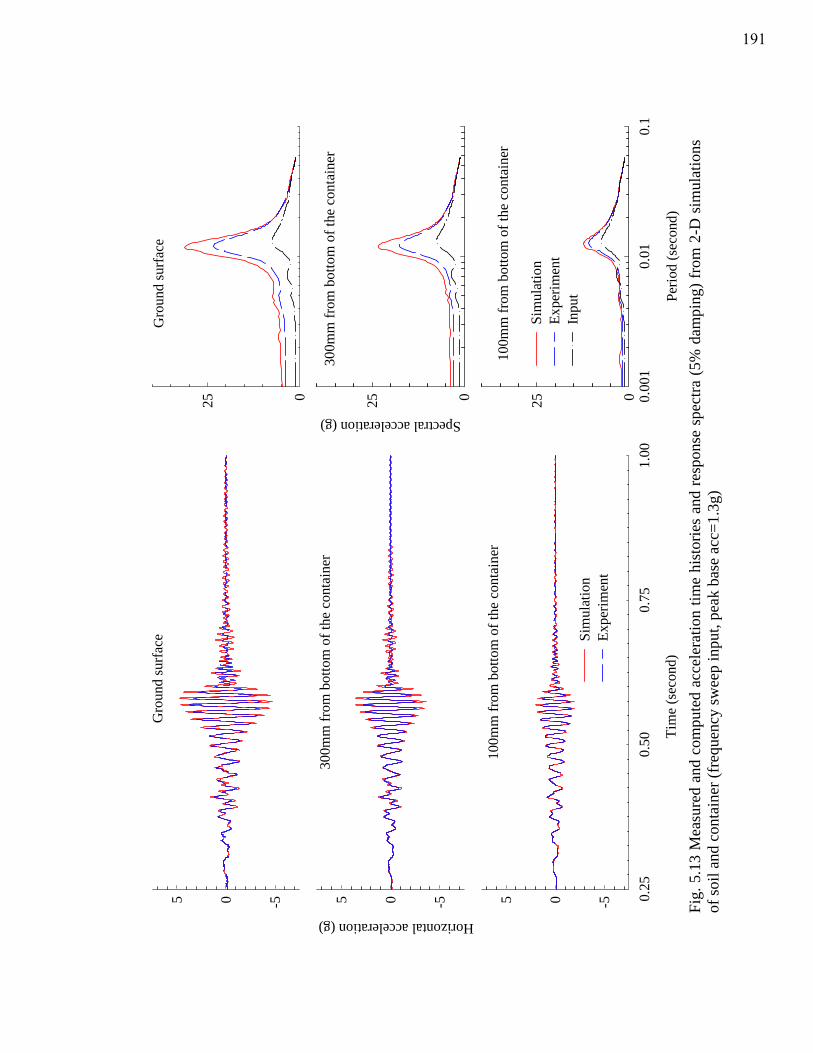
300m
m fr
om b
otto
m o
f the
con
tain
er
Horizontal acceleration (g)
-505
100m
m fr
om b
otto
m o
f the
con
tain
er
Tim
e (s
econ
d)
0.25
0.50
0.75
1.00
-505
Gro
und
surf
ace
-505
Sim
ulat
ion
Expe
rimen
t
Gro
und
surf
ace
025
100m
m fr
om b
otto
m o
f the
con
tain
er
Perio
d (s
econ
d)
0.00
10.
010.
1025
300m
m fr
om b
otto
m o
f the
con
tain
er
Spectral acceleration (g)
025
Sim
ulat
ion
Expe
rimen
tIn
put
Fig.
5.1
3 M
easu
red
and
com
pute
d ac
cele
ratio
n tim
e hi
stor
ies
and
resp
onse
spe
ctra
(5%
dam
ping
) fro
m 2
-D s
imul
atio
ns
of so
il an
d co
ntai
ner (
freq
uenc
y sw
eep
inpu
t, pe
ak b
ase
acc=
1.3g
)
191
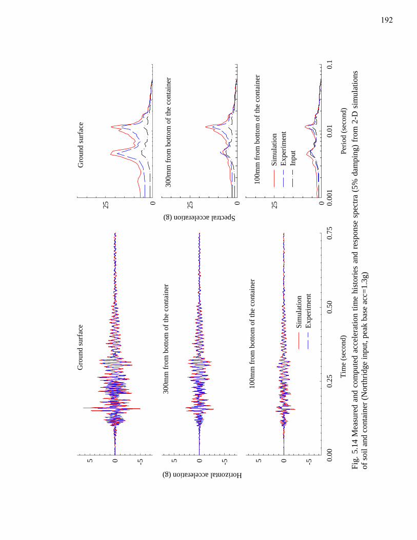
300m
m fr
om b
otto
m o
f the
con
tain
er
Horizontal acceleration (g)
-505
100m
m fr
om b
otto
m o
f the
con
tain
er
Tim
e (s
econ
d)
0.00
0.25
0.50
0.75
-505
Gro
und
surf
ace
-505
Sim
ulat
ion
Expe
rimen
t
Gro
und
surf
ace
025
100m
m fr
om b
otto
m o
f the
con
tain
er
Perio
d (s
econ
d)
0.00
10.
010.
1025
300m
m fr
om b
otto
m o
f the
con
tain
er
Spectral acceleration (g)
025
Sim
ulat
ion
Expe
rimen
tIn
put
Fig.
5.1
4 M
easu
red
and
com
pute
d ac
cele
ratio
n tim
e hi
stor
ies
and
resp
onse
spe
ctra
(5%
dam
ping
) fro
m 2
-D s
imul
atio
ns
of so
il an
d co
ntai
ner (
Nor
thrid
ge in
put,
peak
bas
e ac
c=1.
3g)
192
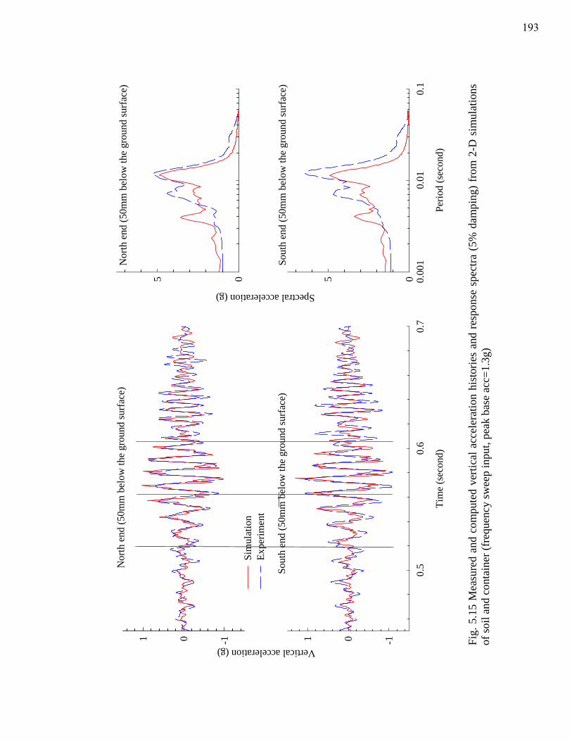
Nor
th e
nd (5
0mm
bel
ow th
e gr
ound
surf
ace)
Spectral acceleration (g)
05
Tim
e (s
econ
d)
0.5
0.6
0.7
-101
Nor
th e
nd (5
0mm
bel
ow th
e gr
ound
surf
ace)
Vertical acceleration (g) -101
Sim
ulat
ion
Expe
rimen
t
Sout
h en
d (5
0mm
bel
ow th
e gr
ound
surf
ace)
Perio
d (s
econ
d)
0.00
10.
010.
105
Sout
h en
d (5
0mm
bel
ow th
e gr
ound
surf
ace)
Fig.
5.1
5 M
easu
red
and
com
pute
d ve
rtica
l acc
eler
atio
n hi
stor
ies
and
resp
onse
spe
ctra
(5%
dam
ping
) fro
m 2
-D s
imul
atio
ns
of so
il an
d co
ntai
ner (
freq
uenc
y sw
eep
inpu
t, pe
ak b
ase
acc=
1.3g
)
193
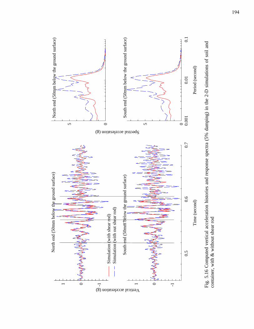
Nor
th e
nd (5
0mm
bel
ow th
e gr
ound
surf
ace)
Spectral acceleration (g)
05
Tim
e (s
econ
d)
0.5
0.6
0.7
-101
Nor
th e
nd (5
0mm
bel
ow th
e gr
ound
surf
ace)
Vertical acceleration (g) -101
Sim
ulat
ion
(with
shea
r rod
)Si
mul
atio
n (w
ith o
ut sh
ear r
od)
Sout
h en
d (5
0mm
bel
ow th
e gr
ound
surf
ace)
Perio
d (s
econ
d)
0.00
10.
010.
105
Sout
h en
d (5
0mm
bel
ow th
e gr
ound
surf
ace)
Fig.
5.1
6 C
ompu
ted
verti
cal a
ccel
erat
ion
hist
orie
s an
d re
spon
se s
pect
ra (
5% d
ampi
ng)
in th
e 2-
D s
imul
atio
ns o
f so
il an
d co
ntai
ner,
with
& w
ithou
t she
ar ro
d
194
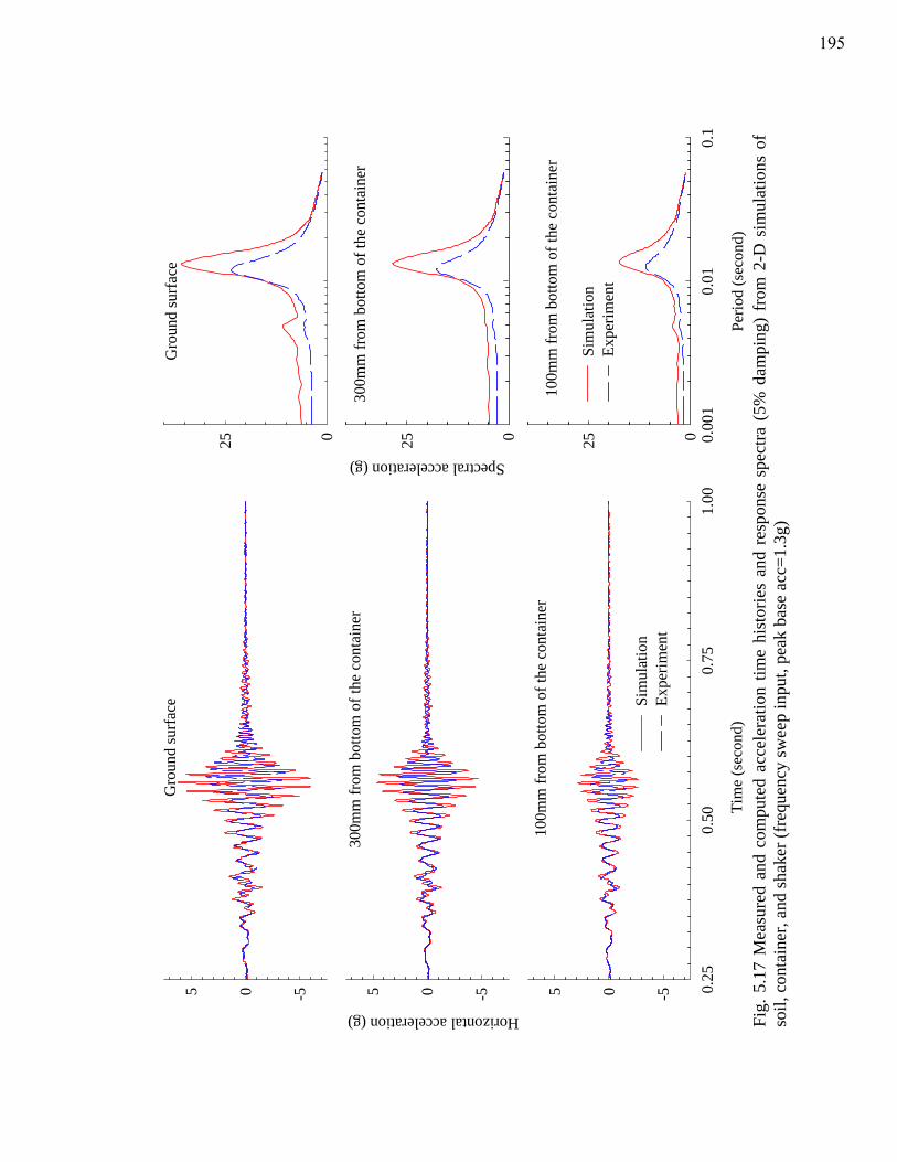
300m
m fr
om b
otto
m o
f the
con
tain
er
Horizontal acceleration (g)
-505
100m
m fr
om b
otto
m o
f the
con
tain
er
Tim
e (s
econ
d)
0.25
0.50
0.75
1.00
-505
Gro
und
surf
ace
-505
Sim
ulat
ion
Expe
rimen
t
Gro
und
surf
ace
025
100m
m fr
om b
otto
m o
f the
con
tain
er
Perio
d (s
econ
d)
0.00
10.
010.
1025
300m
m fr
om b
otto
m o
f the
con
tain
er
Spectral acceleration (g)
025
Sim
ulat
ion
Expe
rimen
t
Fig.
5.1
7 M
easu
red
and
com
pute
d ac
cele
ratio
n tim
e hi
stor
ies
and
resp
onse
spe
ctra
(5%
dam
ping
) fr
om 2
-D s
imul
atio
ns o
f so
il, c
onta
iner
, and
shak
er (f
requ
ency
swee
p in
put,
peak
bas
e ac
c=1.
3g)
195
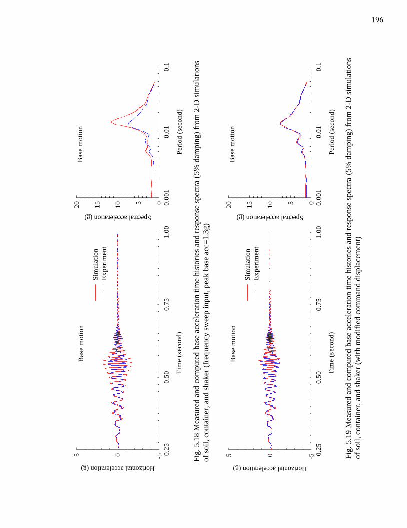
Bas
e m
otio
n
Tim
e (s
econ
d)
0.25
0.50
0.75
1.00
Horizontal acceleration (g)
-505
Sim
ulat
ion
Expe
rimen
t
Bas
e m
otio
n
Perio
d (s
econ
d)
0.00
10.
010.
1
Spectral acceleration (g)
05101520
Fig.
5.1
8 M
easu
red
and
com
pute
d ba
se a
ccel
erat
ion
time
hist
orie
s an
d re
spon
se s
pect
ra (5
% d
ampi
ng) f
rom
2-D
sim
ulat
ions
of
soil,
con
tain
er, a
nd sh
aker
(fre
quen
cy sw
eep
inpu
t, pe
ak b
ase
acc=
1.3g
)
Bas
e m
otio
n
Tim
e (s
econ
d)
0.25
0.50
0.75
1.00
Horizontal acceleration (g)
-505
Sim
ulat
ion
Expe
rimen
t
Bas
e m
otio
n
Perio
d (s
econ
d)
0.00
10.
010.
1Spectral acceleration (g)
05101520
Fig.
5.1
9 M
easu
red
and
com
pute
d ba
se a
ccel
erat
ion
time
hist
orie
s an
d re
spon
se s
pect
ra (5
% d
ampi
ng) f
rom
2-D
sim
ulat
ions
of
soil,
con
tain
er, a
nd sh
aker
(with
mod
ified
com
man
d di
spla
cem
ent)
196
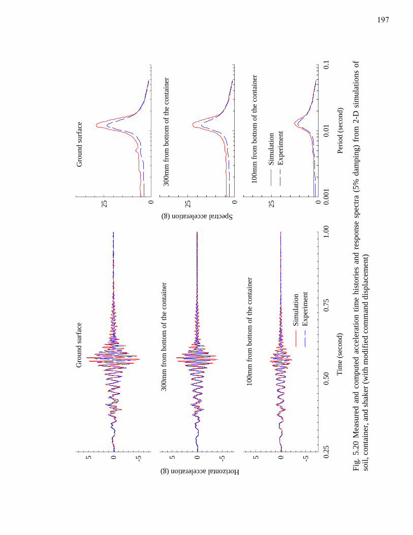
300m
m fr
om b
otto
m o
f the
con
tain
er
Horizontal acceleration (g)
-505
100m
m fr
om b
otto
m o
f the
con
tain
er
Tim
e (s
econ
d)
0.25
0.50
0.75
1.00
-505
Gro
und
surf
ace
-505
Sim
ulat
ion
Expe
rimen
t
Gro
und
surf
ace
025
100m
m fr
om b
otto
m o
f the
con
tain
er
Perio
d (s
econ
d)
0.00
10.
010.
1025
300m
m fr
om b
otto
m o
f the
con
tain
er
Spectral acceleration (g)
025
Sim
ulat
ion
Expe
rimen
t
Fig.
5.2
0 M
easu
red
and
com
pute
d ac
cele
ratio
n tim
e hi
stor
ies
and
resp
onse
spe
ctra
(5%
dam
ping
) fr
om 2
-D s
imul
atio
ns o
f so
il, c
onta
iner
, and
shak
er (w
ith m
odifi
ed c
omm
and
disp
lace
men
t)
197
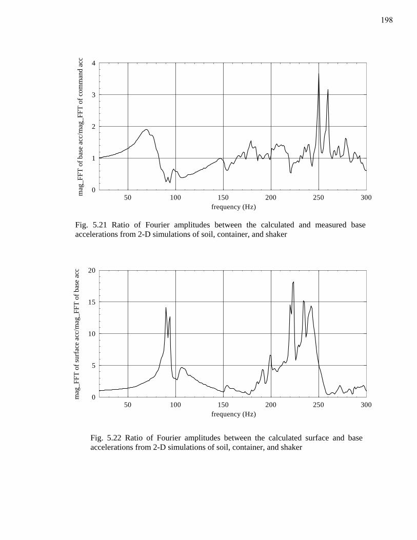
frequency (Hz)50 100 150 200 250 300m
ag_F
FT o
f bas
e ac
c/m
ag_F
FT o
f com
man
d ac
c
0
1
2
3
4
Fig. 5.21 Ratio of Fourier amplitudes between the calculated and measured base accelerations from 2-D simulations of soil, container, and shaker
frequency (Hz)50 100 150 200 250 300
mag
_FFT
of s
urfa
ce a
cc/m
ag_F
FT o
f bas
e ac
c
0
5
10
15
20
Fig. 5.22 Ratio of Fourier amplitudes between the calculated surface and base accelerations from 2-D simulations of soil, container, and shaker
198
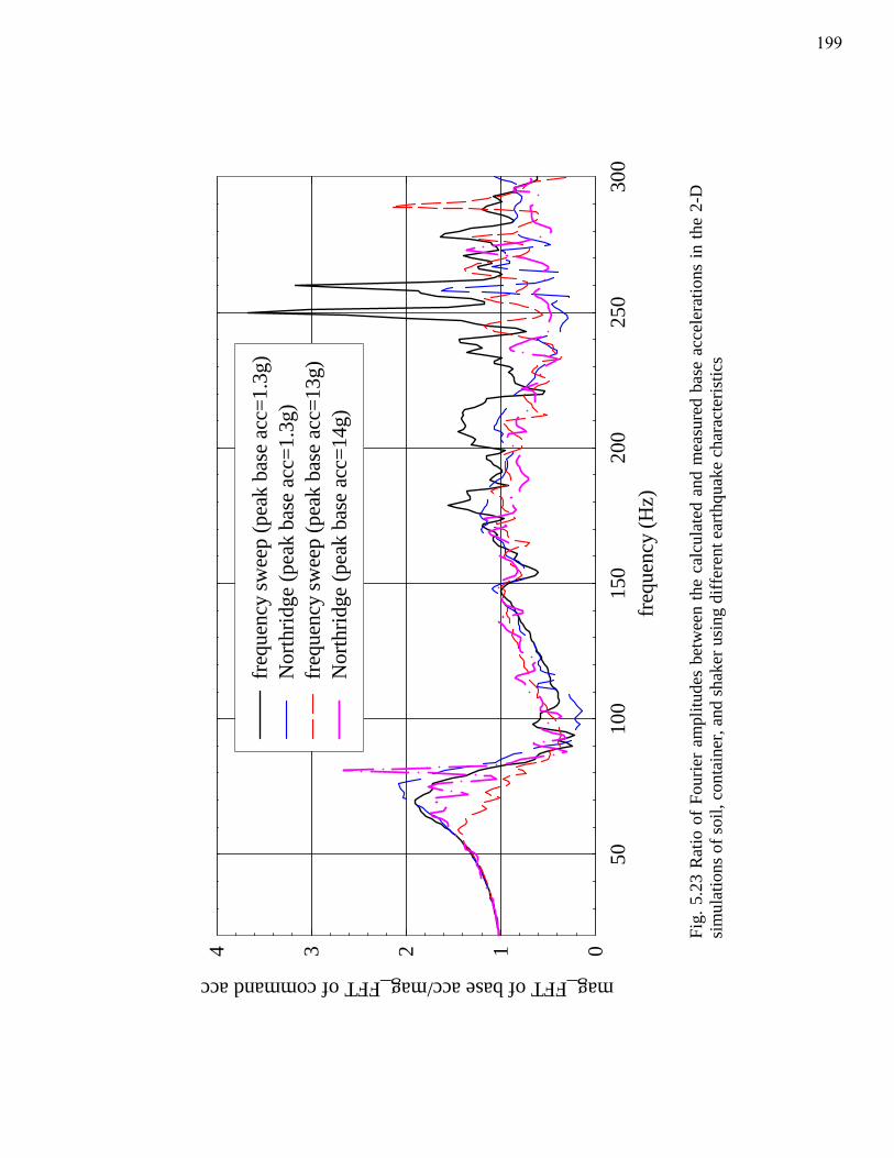
freq
uenc
y (H
z)50
100
150
200
250
300
mag_FFT of base acc/mag_FFT of command acc
01234
freq
uenc
y sw
eep
(pea
k ba
se a
cc=1
.3g)
Nor
thrid
ge (p
eak
base
acc
=1.3
g)fr
eque
ncy
swee
p (p
eak
base
acc
=13g
)N
orth
ridge
(pea
k ba
se a
cc=1
4g)
Fig.
5.2
3 R
atio
of
Four
ier
ampl
itude
s be
twee
n th
e ca
lcul
ated
and
mea
sure
d ba
se a
ccel
erat
ions
in th
e 2-
D
sim
ulat
ions
of s
oil,
cont
aine
r, an
d sh
aker
usi
ng d
iffer
ent e
arth
quak
e ch
arac
teris
tics
199
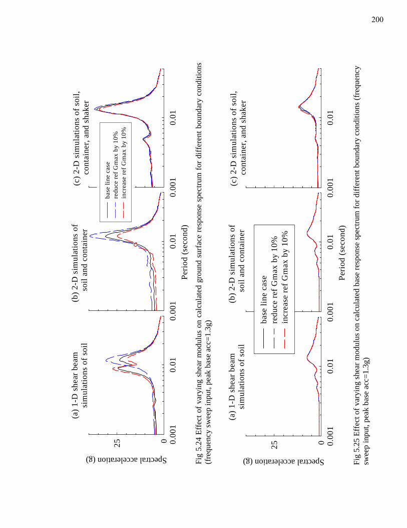
(c) 2
-D s
imul
atio
ns o
f soi
l,
con
tain
er, a
nd s
hake
r
0.00
10.
01
(a) 1
-D s
hear
bea
m
s
imul
atio
ns o
f soi
l
0.00
10.
01025
(b) 2
-D s
imul
atio
ns o
f
soi
l and
con
tain
er
Perio
d (s
econ
d)0.
001
0.01
Spectral acceleration (g)
base
line
cas
ere
duce
ref G
max
by
10%
incr
ease
ref G
max
by
10%
Fig
5.24
Eff
ect o
f var
ying
she
ar m
odul
us o
n ca
lcul
ated
gro
und
surf
ace
resp
onse
spe
ctru
m fo
r diff
eren
t bou
ndar
y co
nditi
ons
(fre
quen
cy sw
eep
inpu
t, pe
ak b
ase
acc=
1.3g
)
(c) 2
-D s
imul
atio
ns o
f soi
l,
con
tain
er, a
nd s
hake
r
0.00
10.
01
(a) 1
-D s
hear
bea
m
s
imul
atio
ns o
f soi
l
0.00
10.
01025
(b) 2
-D s
imul
atio
ns o
f
soi
l and
con
tain
er
Perio
d (s
econ
d)0.
001
0.01
Spectral acceleration (g)
base
line
cas
ere
duce
ref G
max
by
10%
incr
ease
ref G
max
by
10%
Fig
5.25
Eff
ect o
f var
ying
shea
r mod
ulus
on
calc
ulat
ed b
ase
resp
onse
spec
trum
for d
iffer
ent b
ound
ary
cond
ition
s (fr
eque
ncy
swee
p in
put,
peak
bas
e ac
c=1.
3g)
200
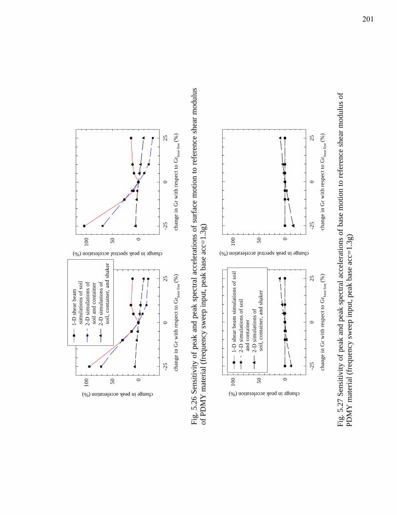
chan
ge in
Gr w
ith re
spec
t to
Gr ba
se li
ne (%
)
-25
025
change in peak spectral acceleration (%)
050100
chan
ge in
Gr w
ith re
spec
t to
Gr ba
se li
ne (%
)
-25
025
change in peak acceleration (%)
050100
1-D
she
ar b
eam
sim
ulat
ions
of s
oil
2-D
sim
ulat
ions
of
soi
l and
con
tain
er2-
D s
imul
atio
ns o
f s
oil,
cont
aine
r, an
d sh
aker
Fig.
5.2
6 Se
nsiti
vity
of p
eak
and
peak
spe
ctra
l acc
eler
atio
ns o
f sur
face
mot
ion
to re
fere
nce
shea
r mod
ulus
of
PD
MY
mat
eria
l (fr
eque
ncy
swee
p in
put,
peak
bas
e ac
c=1.
3g)
chan
ge in
Gr w
ith re
spec
t to
Gr ba
se li
ne (%
)
-25
025
change in peak spectral acceleration (%)
050100
chan
ge in
Gr w
ith re
spec
t to
Gr ba
se li
ne (%
)
-25
025
change in peak acceleration (%)
050100
1-D
she
ar b
eam
sim
ulat
ions
of s
oil
2-D
sim
ulat
ions
of s
oil
and
con
tain
er2-
D s
imul
atio
ns o
f s
oil,
cont
aine
r, an
d sh
aker
Fig.
5.2
7 Se
nsiti
vity
of p
eak
and
peak
spe
ctra
l acc
eler
atio
ns o
f bas
e m
otio
n to
refe
renc
e sh
ear m
odul
us o
f PD
MY
mat
eria
l (fr
eque
ncy
swee
p in
put,
peak
bas
e ac
c=1.
3g)
201
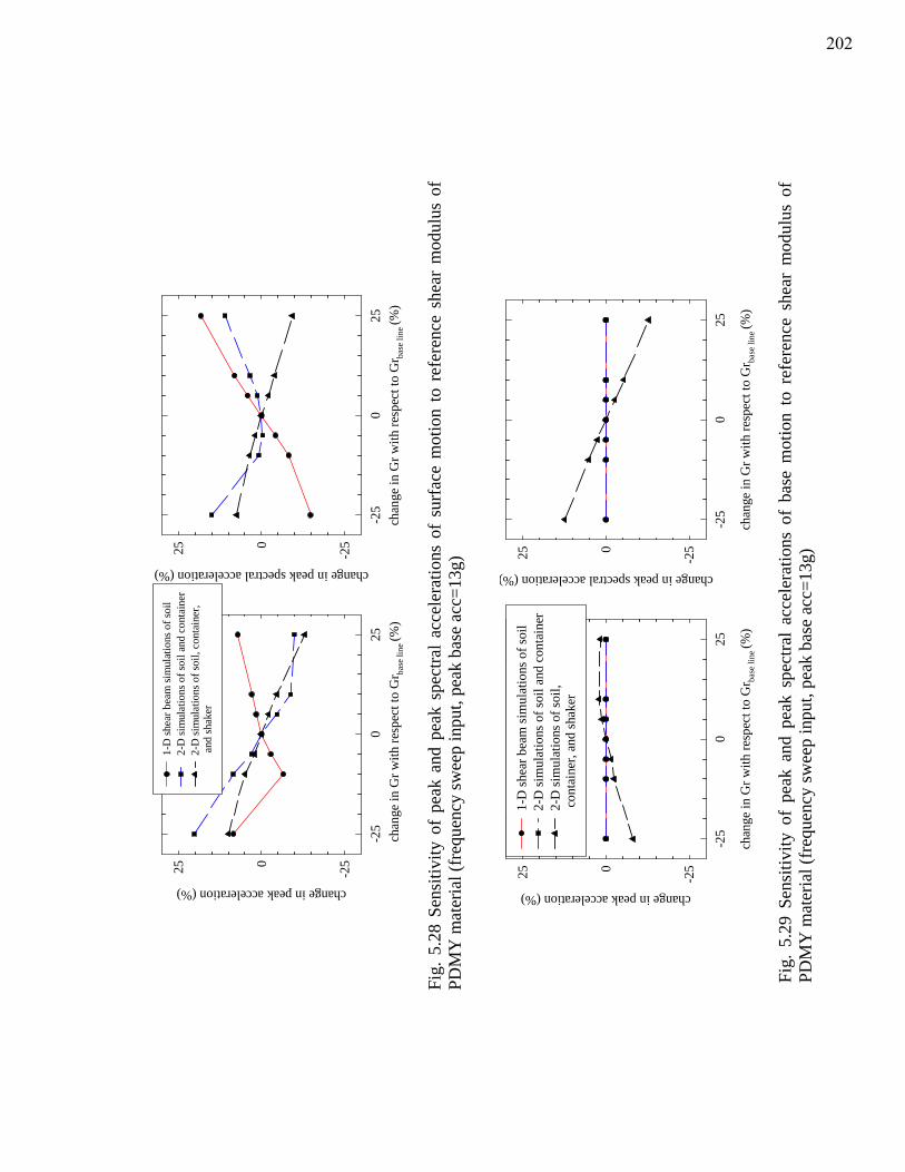
chan
ge in
Gr w
ith re
spec
t to
Gr ba
se li
ne (%
)-2
50
25
change in peak spectral acceleration (%)
-25025
chan
ge in
Gr w
ith re
spec
t to
Gr ba
se li
ne (%
)-2
50
25
change in peak acceleration (%)
-25025
1-D
shea
r bea
m si
mul
atio
ns o
f soi
l2-
D si
mul
atio
ns o
f soi
l and
con
tain
er2-
D si
mul
atio
ns o
f soi
l, co
ntai
ner,
and
shak
er
Fig.
5.2
8 Se
nsiti
vity
of
peak
and
pea
k sp
ectra
l acc
eler
atio
ns o
f su
rfac
e m
otio
n to
ref
eren
ce s
hear
mod
ulus
of
PDM
Y m
ater
ial (
freq
uenc
y sw
eep
inpu
t, pe
ak b
ase
acc=
13g)
chan
ge in
Gr w
ith re
spec
t to
Gr ba
se li
ne (%
)
-25
025
change in peak spectral acceleration (%)
-25025
chan
ge in
Gr w
ith re
spec
t to
Gr ba
se li
ne (%
)
-25
025
change in peak acceleration (%)
-25025
1-D
shea
r bea
m si
mul
atio
ns o
f soi
l2-
D si
mul
atio
ns o
f soi
l and
con
tain
er2-
D si
mul
atio
ns o
f soi
l, c
onta
iner
, and
shak
er
Fig.
5.2
9 Se
nsiti
vity
of
peak
and
pea
k sp
ectra
l ac
cele
ratio
ns o
f ba
se m
otio
n to
ref
eren
ce s
hear
mod
ulus
of
PDM
Y m
ater
ial (
freq
uenc
y sw
eep
inpu
t, pe
ak b
ase
acc=
13g)
202
Chapter 6
Towards developing a numerical model of a servo-hydraulic
centrifuge actuation system to predict shaking table response
This chapter presents a study on the modeling of a servo-hydraulic centrifuge
actuation system with a goal of predicting shaking table response prior to the experiment
for a target earthquake motion. First, the functioning of different components and the
factors affecting the performance of a servo-hydraulic actuation are addressed using an
example analytical model of the servo-hydraulic actuation system available in the
literature. Second, the actuation mechanism of the UC Davis centrifuge horizontal
shaking table system and the details of base motion tuning procedures are briefly
described. Third, an OpenSees numerical model of this actuation system and typical
results from the numerical simulations are presented. Finally, the simulation results and
the need for additional work on this numerical modeling are discussed.
203
6.1 Factors affecting the reproduction of a dynamic signal in a servo-hydraulic
actuation system
In a typical shaking table experiment, an actuator command displacement (could
be a dynamic signal obtained from a real earthquake recording or created by combining
sinusoidal wave forms) is specified to a servo controller and the response of the shaking
table is measured as an output. The degree of distortion between the input command and
the measured output depends on many factors such as characteristics of the test specimen,
physical system parameters (e.g. compliance of reaction mass, compressibility of oil
column in the actuator chamber, oil leakage through the actuator seals, non-linear flow
characteristics in the actuator, servo valve time delay, etc), and configuration and
characteristics of control loops (e.g. type of control algorithm, feedback signals,
dynamics of sensors measuring the feedback response, signal conditioning,
characteristics of the digital data acquisition and control system, anti-aliasing filters,
control gain setting, etc) (Conte et al. 2000). Therefore to evaluate the capability of the
actuation system in reproducing base motions (measured motions at shaking table), it is
important to understand the effects of above factors on the performance of the actuation
system under wide range of test configurations and operation conditions. Furthermore, a
thorough understanding of the performance of the actuation system is essential for the
proper design of loading protocols (ground motion characteristics) in the experiment,
proper interpretation of experimental results, and for the safety of the equipment.
204
6.2 Analytical models for various components of servo-hydraulic actuation
system
Various analytical models to capture the salient features different components of
the servo-hydraulic actuation system (such as actuator, servo valve, controller, etc.) are
available in the literature for structural shaking table experiments and real-time pseudo
dynamic testing in the context of structural engineering (Conte et al. 2000, Williams et al.
2001, and Jung et al. 2006). To improve our understanding of functions and modeling
issues of diffent components of the servo-hydraulic actuation system, it is worth looking
at one of the examples from above literature.
A linear analytical model of a uni-axial, displacement controlled shaking table
system, presented by Conte et al. (2000), is depicted in Fig. 6.1 and briefly described
below. As indicated in Fig. 6.1, the analytical model is developed following the modular
approach in the form of ‘Shaking Table Transfer Function’ (T(s) in Laplace domain)
between desired (or commanded) and actual absolute shaking table motions. This
modular approach breaks down the shaking table system into several subsystems.
i) Three-stage servo valve transfer function, Ht(s)
Functioning (characterized by an ‘inner feedback control loop) and the analytical
model of the three-stage servo valve transfer function are schematically shown in Fig.
6.2. As shown in Fig. 6.2, the servo valve command signal, xc(s), before being sent to the
first stage of the servo valve, is processed by the inner control loop in order to yield the
inner loop conditioned servo valve command signal, xci(s). The electric signal, xci(s),
controls the rotation of the pilot flapper which generates a differential pressure in the
pilot stage (or second stage), ΔPp(s). The differential pressure ΔPp(s) thus created controls
205
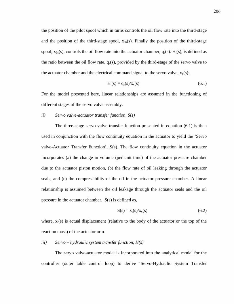
the position of the pilot spool which in turns controls the oil flow rate into the third-stage
and the position of the third-stage spool, x3s(s). Finally the position of the third-stage
spool, x3s(s), controls the oil flow rate into the actuator chamber, qs(s). Ht(s), is defined as
the ratio between the oil flow rate, qs(s), provided by the third-stage of the servo valve to
the actuator chamber and the electrical command signal to the servo valve, xc(s):
Ht(s) = qs(s)/xc(s) (6.1)
For the model presented here, linear relationships are assumed in the functioning of
different stages of the servo valve assembly.
ii) Servo valve-actuator transfer function, S(s)
The three-stage servo valve transfer function presented in equation (6.1) is then
used in conjunction with the flow continuity equation in the actuator to yield the ‘Servo
valve-Actuator Transfer Function’, S(s). The flow continuity equation in the actuator
incorporates (a) the change in volume (per unit time) of the actuator pressure chamber
due to the actuator piston motion, (b) the flow rate of oil leaking through the actuator
seals, and (c) the compressibility of the oil in the actuator pressure chamber. A linear
relationship is assumed between the oil leakage through the actuator seals and the oil
pressure in the actuator chamber. S(s) is defined as,
S(s) = xt(s)/xc(s) (6.2)
where, xt(s) is actual displacement (relative to the body of the actuator or the top of the
reaction mass) of the actuator arm.
iii) Servo – hydraulic system transfer function, H(s)
The servo valve-actuator model is incorporated into the analytical model for the
controller (outer table control loop) to derive ‘Servo-Hydraulic System Transfer
206
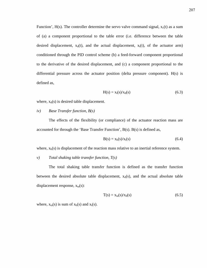
Function’, H(s). The controller determine the servo valve command signal, xc(t) as a sum
of (a) a component proportional to the table error (i.e. difference between the table
desired displacement, xd(t), and the actual displacement, xt(t), of the actuator arm)
conditioned through the PID control scheme (b) a feed-forward component proportional
to the derivative of the desired displacement, and (c) a component proportional to the
differential pressure across the actuator position (delta pressure component). H(s) is
defined as,
H(s) = xt(s)/xd(s) (6.3)
where, xd(s) is desired table displacement.
iv) Base Transfer function, B(s)
The effects of the flexibility (or compliance) of the actuator reaction mass are
accounted for through the ‘Base Transfer Function’, B(s). B(s) is defined as,
B(s) = xb(s)/xt(s) (6.4)
where, xb(s) is displacement of the reaction mass relative to an inertial reference system.
v) Total shaking table transfer function, T(s)
The total shaking table transfer function is defined as the transfer function
between the desired absolute table displacement, xd(s), and the actual absolute table
displacement response, xta(s):
T(s) = xta(s)/xd(s) (6.5)
where, xta(s) is sum of xb(s) and xt(s).
207
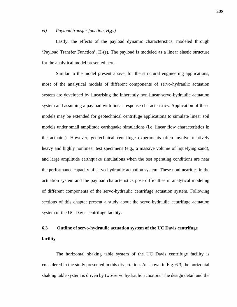
vi) Payload transfer function, Hp(s)
Lastly, the effects of the payload dynamic characteristics, modeled through
‘Payload Transfer Function’, Hp(s). The payload is modeled as a linear elastic structure
for the analytical model presented here.
Similar to the model present above, for the structural engineering applications,
most of the analytical models of different components of servo-hydraulic actuation
system are developed by linearising the inherently non-linear servo-hydraulic actuation
system and assuming a payload with linear response characteristics. Application of these
models may be extended for geotechnical centrifuge applications to simulate linear soil
models under small amplitude earthquake simulations (i.e. linear flow characteristics in
the actuator). However, geotechnical centrifuge experiments often involve relatively
heavy and highly nonlinear test specimens (e.g., a massive volume of liquefying sand),
and large amplitude earthquake simulations when the test operating conditions are near
the performance capacity of servo-hydraulic actuation system. These nonlinearities in the
actuation system and the payload characteristics pose difficulties in analytical modeling
of different components of the servo-hydraulic centrifuge actuation system. Following
sections of this chapter present a study about the servo-hydraulic centrifuge actuation
system of the UC Davis centrifuge facility.
6.3 Outline of servo-hydraulic actuation system of the UC Davis centrifuge
facility
The horizontal shaking table system of the UC Davis centrifuge facility is
considered in the study presented in this dissertation. As shown in Fig. 6.3, the horizontal
shaking table system is driven by two-servo hydraulic actuators. The design detail and the
208
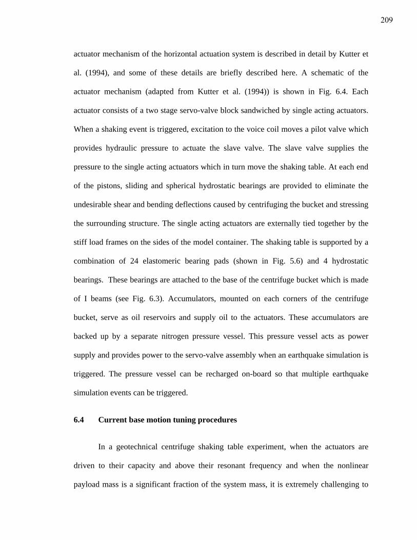
actuator mechanism of the horizontal actuation system is described in detail by Kutter et
al. (1994), and some of these details are briefly described here. A schematic of the
actuator mechanism (adapted from Kutter et al. (1994)) is shown in Fig. 6.4. Each
actuator consists of a two stage servo-valve block sandwiched by single acting actuators.
When a shaking event is triggered, excitation to the voice coil moves a pilot valve which
provides hydraulic pressure to actuate the slave valve. The slave valve supplies the
pressure to the single acting actuators which in turn move the shaking table. At each end
of the pistons, sliding and spherical hydrostatic bearings are provided to eliminate the
undesirable shear and bending deflections caused by centrifuging the bucket and stressing
the surrounding structure. The single acting actuators are externally tied together by the
stiff load frames on the sides of the model container. The shaking table is supported by a
combination of 24 elastomeric bearing pads (shown in Fig. 5.6) and 4 hydrostatic
bearings. These bearings are attached to the base of the centrifuge bucket which is made
of I beams (see Fig. 6.3). Accumulators, mounted on each corners of the centrifuge
bucket, serve as oil reservoirs and supply oil to the actuators. These accumulators are
backed up by a separate nitrogen pressure vessel. This pressure vessel acts as power
supply and provides power to the servo-valve assembly when an earthquake simulation is
triggered. The pressure vessel can be recharged on-board so that multiple earthquake
simulation events can be triggered.
6.4 Current base motion tuning procedures
In a geotechnical centrifuge shaking table experiment, when the actuators are
driven to their capacity and above their resonant frequency and when the nonlinear
payload mass is a significant fraction of the system mass, it is extremely challenging to
209
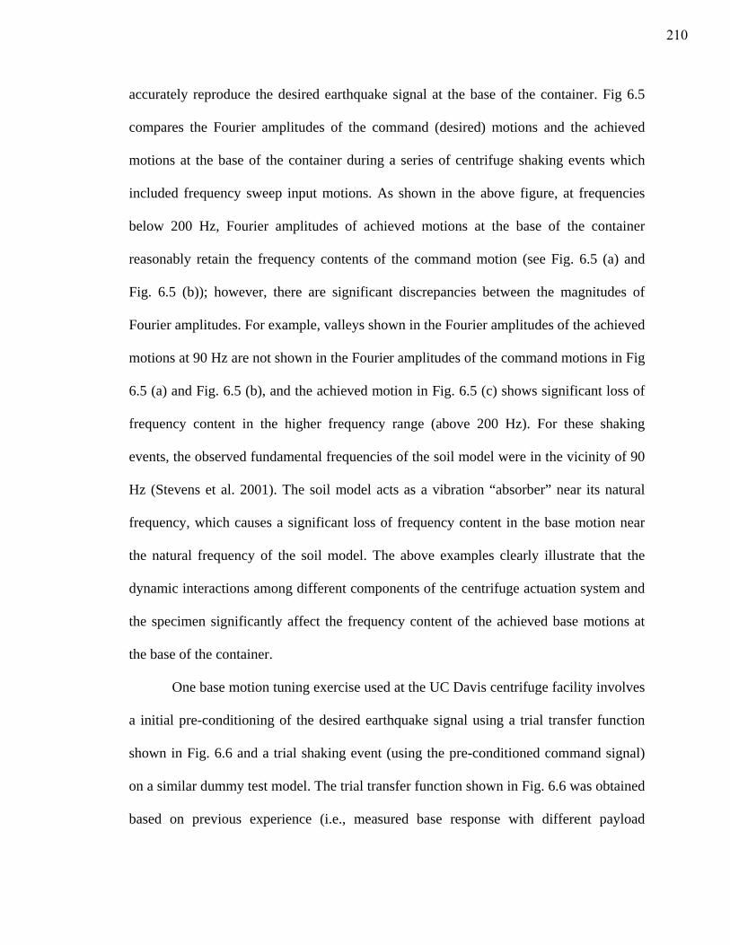
accurately reproduce the desired earthquake signal at the base of the container. Fig 6.5
compares the Fourier amplitudes of the command (desired) motions and the achieved
motions at the base of the container during a series of centrifuge shaking events which
included frequency sweep input motions. As shown in the above figure, at frequencies
below 200 Hz, Fourier amplitudes of achieved motions at the base of the container
reasonably retain the frequency contents of the command motion (see Fig. 6.5 (a) and
Fig. 6.5 (b)); however, there are significant discrepancies between the magnitudes of
Fourier amplitudes. For example, valleys shown in the Fourier amplitudes of the achieved
motions at 90 Hz are not shown in the Fourier amplitudes of the command motions in Fig
6.5 (a) and Fig. 6.5 (b), and the achieved motion in Fig. 6.5 (c) shows significant loss of
frequency content in the higher frequency range (above 200 Hz). For these shaking
events, the observed fundamental frequencies of the soil model were in the vicinity of 90
Hz (Stevens et al. 2001). The soil model acts as a vibration “absorber” near its natural
frequency, which causes a significant loss of frequency content in the base motion near
the natural frequency of the soil model. The above examples clearly illustrate that the
dynamic interactions among different components of the centrifuge actuation system and
the specimen significantly affect the frequency content of the achieved base motions at
the base of the container.
One base motion tuning exercise used at the UC Davis centrifuge facility involves
a initial pre-conditioning of the desired earthquake signal using a trial transfer function
shown in Fig. 6.6 and a trial shaking event (using the pre-conditioned command signal)
on a similar dummy test model. The trial transfer function shown in Fig. 6.6 was obtained
based on previous experience (i.e., measured base response with different payload
210
characteristics and earthquake characteristics) to approximate (linear approximation) the
non-linear behavior of the centrifuge actuation system. The shape of this transfer function
in the lower frequency range (frequencies less than 20 Hz) is derived to minimize the
excitation of the centrifuge arm at its resonant frequencies (i.e., 5 Hz and 20 Hz are 1st
and 2nd bending resonant frequencies of the centrifuge arm, desired earthquake signal at
these frequencies are filtered to a significant amount in Fig. 6.6). Representative base
motion tuning results using this initial preconditioning scheme are presented in Fig. 6.7
and Fig. 6.8, in terms of time histories and the magnitude of the Fourier amplitude
spectrums, respectively. As shown in above figures, for this particular case, peak
accelerations of the target (desired) and the achieved base motions are nearly equal, the
pre-conditioning scheme reasonably capture the locations of peaks and the valleys of FFT
of base motions except in the lower frequency range (frequencies less than 20 Hz were
filtered in the pre-conditioning scheme) and in the higher frequency range (frequencies
higher than 200 Hz). Also, discrepancies between the magnitudes of FFT of base motions
are apparent in Fig. 6.8. If matching target motion at the ground surface or any other
location of the model is important, in addition to the pre-conditioning scheme described
above, further corrections on the achieved base motion are necessary. An example of the
base motion tuning exercise, which included some additional correction procedures to get
a good match with target motion specified at 50 mm below the ground surface within the
test specimen, was presented in section 3.2.6 of this dissertation.
211
6.5 Modifications to the shaker model presented in chapter 5 (depicted in Fig.
5.8)
The shaker model presented in chapter 5 (see Fig. 5.8) employs a simplistic
approximation of the actuator and control system, using the springs and dashpots, to
include the first-order effects of actuator flexibility on the interaction between the test
specimen and the shaking table and it uses the measured container base motion (from
experiment) to develop input command displacement and then the input command force.
Application of this shaker model is extended to accommodate the actual command
displacement, specified to the servo controller (during the experiment), as a command
displacement in the shaker model; so that the base response could be obtained as an
output in the numerical model. Details of these modifications and the results from these
analyses and are presented in the following sections.
6.5.1 To account for the effects of feed-back controller
A simplistic approximation using a mechanical-lever system (BCD in Fig. 6.10) is
added to the original shaker model, with a goal of incorporating the first order effects of
feed-back controller on the command displacement (or command force in the numerical
model). In the OpenSees model, node A (node A is connected to shaking table) is
connected using a rigid link to the node B. BCD is a mechanical-lever system (BC =
CD), it has the pivot point at node C (node C is connected to reaction mass) such that
nodes B and D will have equal but opposite displacement relative to node C. Two
additional stiff springs k3 and k4 are used to account for the effect of controller, which is
proportional to the relative displacement of the shaking table with respect to reaction
212
mass (i.e., x1-x2), on the command displacement. Let’s consider the equation of motions
of the shaker system to further understand the functioning of this mechanical feed-back
system. For this purpose, the payload and reaction mass are represented as lumped
masses (i.e., only to write equation of motion, not in the actual numerical model) in Fig.
6.9 and in Fig. 6.10 and the degrees of freedoms of these lumped masses are indicated in
the above figures. Based on these representations, the equations of motion of the dynamic
system in Fig 6.10 could be written as follows:
0)}()({)]()([ 321421313213211 =+−+−+−−−− xxxkxxkxxkxxcxm &&&& (6.6)
0)}(2)({)]()([ 321421332122 =+−−−−+−+ xxxkxxktFxxkxm com&& (6.7)
0)}({)]()()()([ 321432113213233 =+−+−−−−+−+ xxxktFxxkxxkxxcxm com&&&& (6.8)
In the above equations, the terms inside [ ] are the components from the equation
of motion of the dynamic system shown in Fig. 6.9 and the terms inside { } are the
additional components in the equation of motion due to the addition of mechanical feed-
back system in Fig. 6.10. In the model calibration process, both k3 and k4 are represented
in terms of k1 (k3=k1/10 and k4=k1).
6.5.2 To account for the oil pressure limit and the limit on oil flow velocity
As indicated in Fig. 6.11 (a), a stiff spring, kL (kL = 100k1), and a dashpot, cL, are
added to the shaker model to account for the limit oil pressure and the limit oil flow
velocity. Fig. 6.11 (b) and Fig. 6.11 (c) present the characteristics of kL and cL,
respectively.
213
6.5.3 To account for servo-valve nonlinearity
In Fig. 6.11 (a), a bi-linear spring k1* (across which the input command is
specified) is used to accommodate the effects of non-linearity of the servo-valve on the
simulated shaking table response. The configuration of k1* is depicted in Fig. 6.11 (d).
The purpose of this element is to account for the different behavior of the actuators
during low and high amplitude excitations; the actuators have been observed to perform
better under larger amplitude excitation.
In addition to the above modifications, as mentioned earlier, numerical
simulations are performed by adapting the input force command calculated using the
actual command displacement specified to the servo controller during the experiment.
Typical results from some of these simulations are presented below.
6.6 Simulated base response
A series of shaking event from the centrifuge test series dks02 are considered in
these simulations. These shaking events included a series of frequency sweep input
motions. Dry Nevada sand, placed at a relative density of 100% in a flexible shear beam
model container, was used to model soil in the dks02 test series. Further details of this
experiment can be found in the test series data report Stevens et al. (1999).
Fig. 6.12 compares simulated displacements at the base of container with the
experimental result. Base displacements in the experiment were obtained by double
integrating the accelerations measured at the base of the container. As shown in Fig 6.12,
for this particular input motion, the simulation reasonably captures the steady state
response observed in the experiment (i.e., good match in the displacements in the time
214
range of 0.75 to 1 seconds); however, higher frequency cycles of the displacements (after
1.8 seconds) are poorly predicted by the simulations and the spikes shown at the
beginning and end of the time histories of base displacements in the experiment are not
shown in the simulation results. Fig. 6.13 compares the simulated and the measured base
displacements for the same the frequency sweep input motion (50 to 125 Hz), for
different ‘g’ levels and shaking intensities. In Fig. 6.13 (a) and Fig. 6.13 (c), at 20g level
for two different levels of shaking intensities, simulations reasonably predicted the steady
state displacements obtained from the experiment. Whereas, in Fig. 6.13 (b), at 40g level
for a relatively larger shaking intensity (i.e., Amplification factor for base motion is 2.2),
there are significant discrepancies between the simulated and the measured base
displacements. This suggests that the non-linear response exhibits by the servo-hydraulic
actuation system at a relatively larger shaking intensity is not perfectly modeled in the
shaker model depicted in Fig. 6.11 (a).
Ratios of Fourier amplitudes between the command motion and the achieved base
motions in the experiment and the simulations are shown in Fig. 6.14 for the same event
considered in Fig. 6.12. As indicated in Fig. 6.14, the ratios of Fourier amplitudes
between the command motion and the achieved base motion in the experiment and the
simulation both show peaks around 105 Hz which is close to the experimentally observed
natural frequency (102 Hz) of the soil column (Stevens, 2002). This may be attributable
to the presence of the strong dynamic interaction between the soil model and the
actuation system close to the natural frequency of the soil model. However, the
magnitudes of ratios of Fourier amplitudes are significantly different in the experiment
and the simulation (i.e., scales of y axes off by a factor of 10).
215
For the same frequency sweep input motion, Fig. 6.15 presents the ratios of the
Fourier amplitudes between the command motions and the measured base motions, for
different ‘g’ levels and shaking intensities. As indicated in Fig. 6.15, for different levels
of shaking intensities, ratios of Fourier amplitudes exhibit predominant peaks around 105
Hz and 90 Hz at 40 g and 20 g levels, respectively. These frequencies are close to the
natural frequencies of the soil column at 40 g and 20 g levels, respectively (i.e. for the
linear elastic soil model, frequency is proportional to the confining pressure). At a same
‘g’ level, ratios of Fourier amplitudes show a bigger predominant peak for the lower
intensity motion and a lower predominant peak for the higher intensity motion. In
addition, at a same ‘g’ level, the ratios of Fourier amplitudes are off by a factor of two in
the lower frequency range (50 to 125 Hz) for different levels of shaking intensities
considered. These differences may be attributable to the non-linear behavior of the servo-
hydraulic actuation system (i.e. shaker requires relatively larger input for a smaller
shaking event than a larger shaking event).
Fig. 6.16 presents the ratios of Fourier amplitudes between the command motions
and the simulated base motions for the same events presented in Fig. 6.15. As shown in
Fig. 6.16, at 40 g level, ratios of Fourier amplitudes exhibit peaks close to 105 Hz for
different intensity motions (dks02_w and dks02_bw). In addition, at 20 g level, the
smaller intensity event (dks02_ca) shows a smaller peak at the vicinity of 90 Hz;
whereas, the larger intensity event (dks02_bz), does not show a peak close to this
frequency. At the lower frequency range of the input motion (50 to 75 Hz), the ratios of
Fourier amplitudes are almost identical for different levels of shaking intensities; which is
different from the behavior observed in the experimental results in Fig. 6.15. Further, the
216
magnitudes of ratios of Fourier amplitudes are significantly different in the experiment
and the simulation.
6.7 Discussion on the simulation results and the need for additional work
In the absence OpensSees material models and elements to model various
components of the servo-hydraulic actuation system, a simplistic approximation using
springs and dashpots was used to model the actuator, servo-valve and the control system
in the numerical model of the centrifuge actuation system depicted in Fig. 6.11.
Generally, for the soil model and the frequency sweep input (50 to 125 Hz) considered in
the simulations, the above shaker model reasonably reproduce some features of the base
response observed in the experiment. For example, steady state components of base
displacements were reasonably predicted up to a certain extent in Fig. 6.12 and Fig. 6.13
and, in some cases, the frequencies of the peaks of ratios of Fourier amplitudes (base
transfer functions) between the command and the measured or simulated base motions in
Fig. 6.16 and in Fig. 6.17 were located at the proximity of the experimentally observed
natural frequencies of the soil model. However, the higher frequency components of the
base displacements and the magnitudes of the base transfer functions were poorly
predicted in the simulations. Also, while the results were not presented here, the
simulations using the command motions with significantly higher frequency contents (see
Fig. 6.5 (b) and Fig. 6.5 (c)) resulted in poor predictions of the base displacements and
the base transfer functions.
As described earlier, the degree of distortion between the input command motion
and the measured motion at the shaking table depends on numerous factors such as the
characteristics of the soil model, compressibility of oil column in the actuator, non-linear
217
flow characteristics in the actuator, servo-valve time delay, configuration of control loops
etc. Geotechnical centrifuge experiments often involve highly non-linear test specimens
where the payload mass is a significant fraction of the system mass and the larger
amplitude earthquake simulations where the actuator characteristics are themselves non-
linear. In addition, in the centrifuge experiments frequencies are scaled by the factor of
‘g’ level. The resonant frequencies of higher vibration modes of different components of
the actuation system and the higher frequency responses of the actuator, the servo-valve
and the control system would affect the characteristics (magnitude, frequency content,
and wave form) of the dynamic signal measured at the shaking table. Therefore, to
capture the salient features of the non-linear actuator and servo-valve and to compensate
for the effects of poles and zeros that develop in the feed-back control system on the
shaking table response, it is concluded that more sophisticated analytical models of the
actuator, servo-valve, and controller are required. Development of these advanced
analytical models, especially for the geotechnical centrifuge applications, is a topic for
future research. These analytical models could then be used to model the servo-hydraulic
actuation system to predict the shaking table response in the centrifuge experiments,
involving different characteristics of payload and earthquake motions, and wide range of
test operating conditions.
218
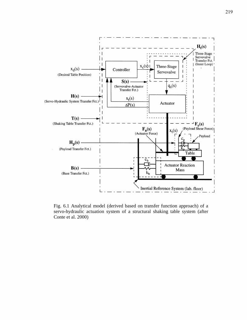
Fig. 6.1 Analytical model (derived based on transfer function approach) of a servo-hydraulic actuation system of a structural shaking table system (after Conte et al. 2000)
219
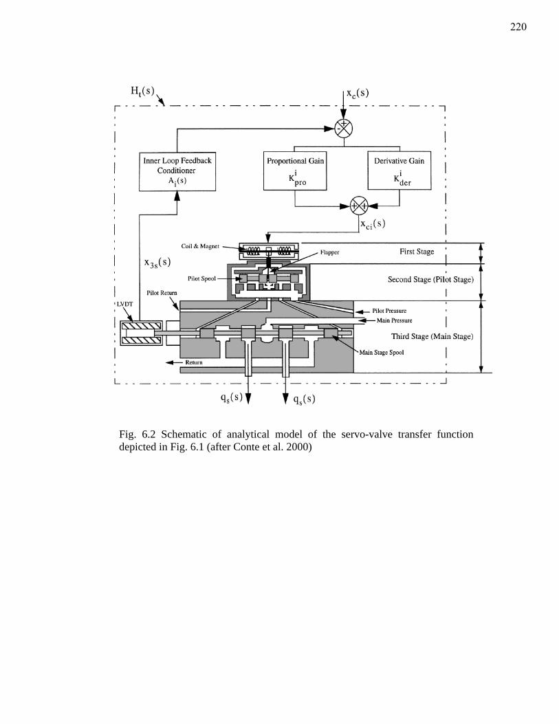
Fig. 6.2 Schematic of analytical model of the servo-valve transfer function depicted in Fig. 6.1 (after Conte et al. 2000)
220

Fig. 6.3 Plan (top) and elevation (bottom) views of the horizontal shaking table system at the UC Davis centrifuge facility (after Kutter at al. 1994)
221
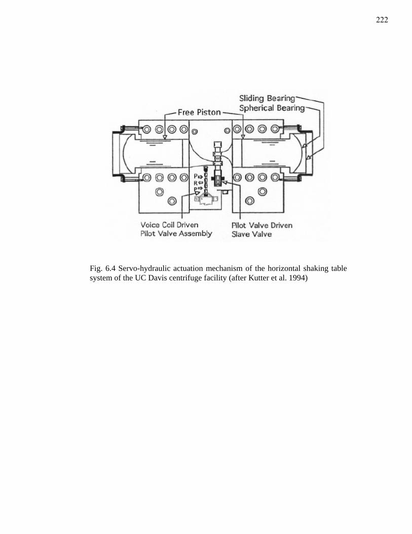
Fig. 6.4 Servo-hydraulic actuation mechanism of the horizontal shaking table system of the UC Davis centrifuge facility (after Kutter et al. 1994)
222
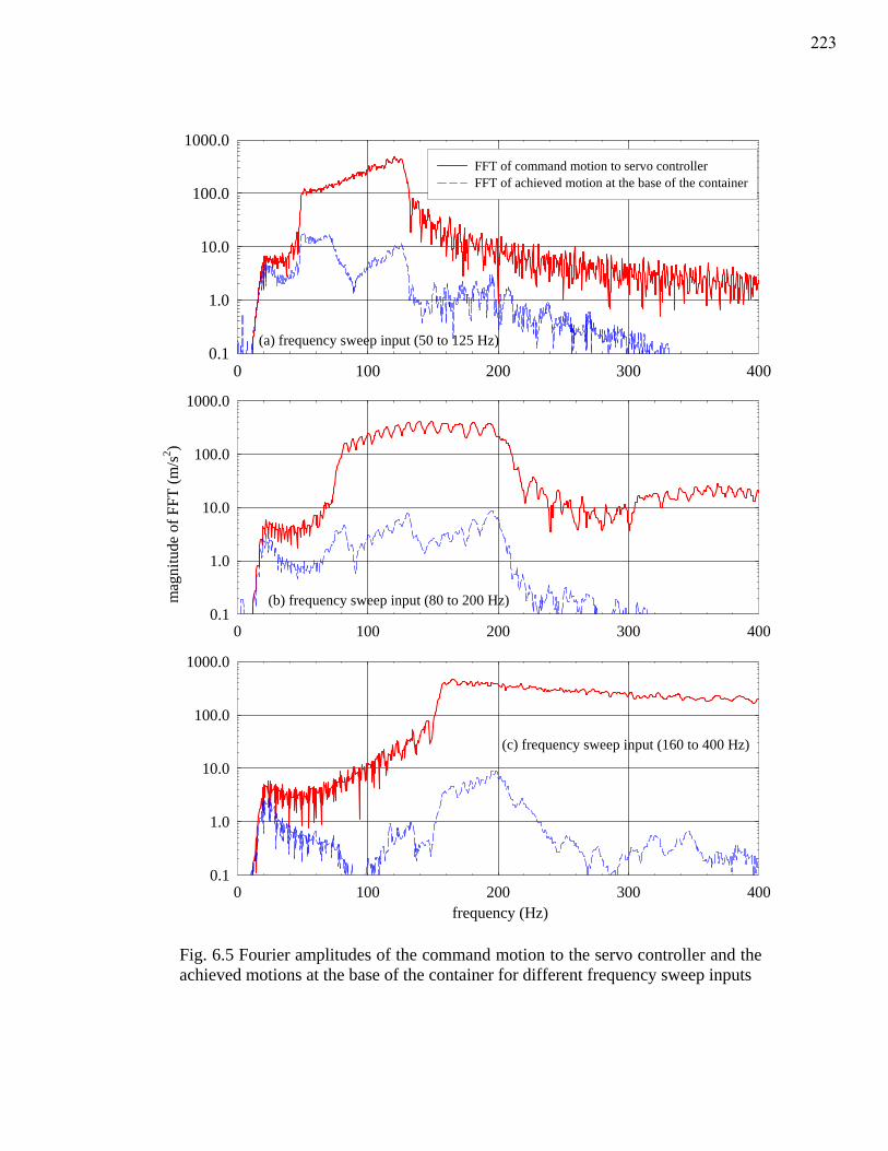
Fig. 6.5 Fourier amplitudes of the command motion to the servo controller and the achieved motions at the base of the container for different frequency sweep inputs
(a) frequency sweep input (50 to 125 Hz)
0 100 200 300 4000.1
1.0
10.0
100.0
1000.0FFT of command motion to servo controllerFFT of achieved motion at the base of the container
(b) frequency sweep input (80 to 200 Hz)
0 100 200 300 400
mag
nitu
de o
f FFT
(m/s
2 )
0.1
1.0
10.0
100.0
1000.0
(c) frequency sweep input (160 to 400 Hz)
frequency (Hz)0 100 200 300 400
0.1
1.0
10.0
100.0
1000.0
223
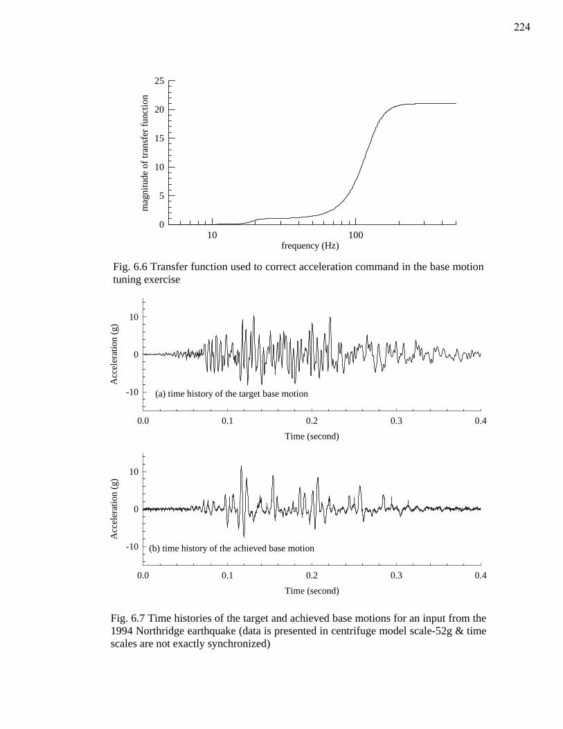
frequency (Hz)10 100
mag
nitu
de o
f tra
nsfe
r fun
ctio
n
0
5
10
15
20
25
Fig. 6.6 Transfer function used to correct acceleration command in the base motion tuning exercise
(a) time history of the target base motion
Time (second)
0.0 0.1 0.2 0.3 0.4
Acc
eler
atio
n (g
)
-10
0
10
(b) time history of the achieved base motion
Time (second)
0.0 0.1 0.2 0.3 0.4
Acc
eler
atio
n (g
)
-10
0
10
Fig. 6.7 Time histories of the target and achieved base motions for an input from the 1994 Northridge earthquake (data is presented in centrifuge model scale-52g & time scales are not exactly synchronized)
224
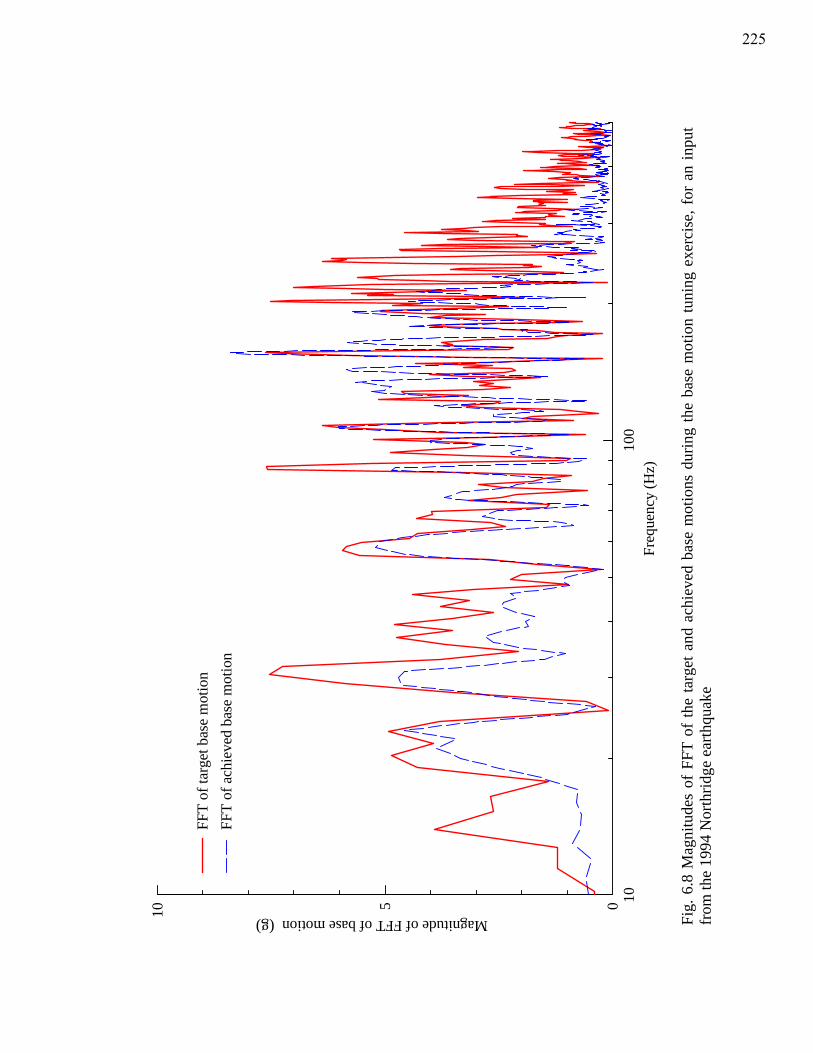
Freq
uenc
y (H
z)10
100
Magnitude of FFT of base motion
0510
FFT
of ta
rget
bas
e m
otio
nFF
T of
ach
ieve
d ba
se m
otio
n
Fig.
6.8
Mag
nitu
des
of F
FT o
f th
e ta
rget
and
ach
ieve
d ba
se m
otio
ns d
urin
g th
e ba
se m
otio
n tu
ning
exe
rcis
e, f
or a
n in
put
from
the
1994
Nor
thrid
ge e
arth
quak
e
(g)
225
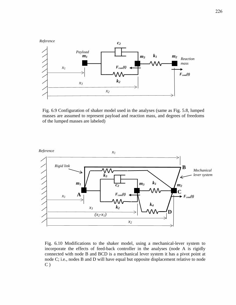
k2
c2
k1 m1 m2 m3
x3
Fcom(t) x1
x2
Reference
Reaction mass
Payload
Fcom(t)
Fig. 6.9 Configuration of shaker model used in the analyses (same as Fig. 5.8, lumped masses are assumed to represent payload and reaction mass, and degrees of freedoms of the lumped masses are labeled)
k2
c2 k1 m2 m3
Fcom(t) x1
Reference
Mechanical lever system
Fcom(t)
x3
x2 (x2-x1)
x1
m1
Rigid link
k4
k3
A
B
C
D
Fig. 6.10 Modifications to the shaker model, using a mechanical-lever system to incorporate the effects of feed-back controller in the analyses (node A is rigidly connected with node B and BCD is a mechanical lever system it has a pivot point at node C; i.e., nodes B and D will have equal but opposite displacement relative to node C )
226
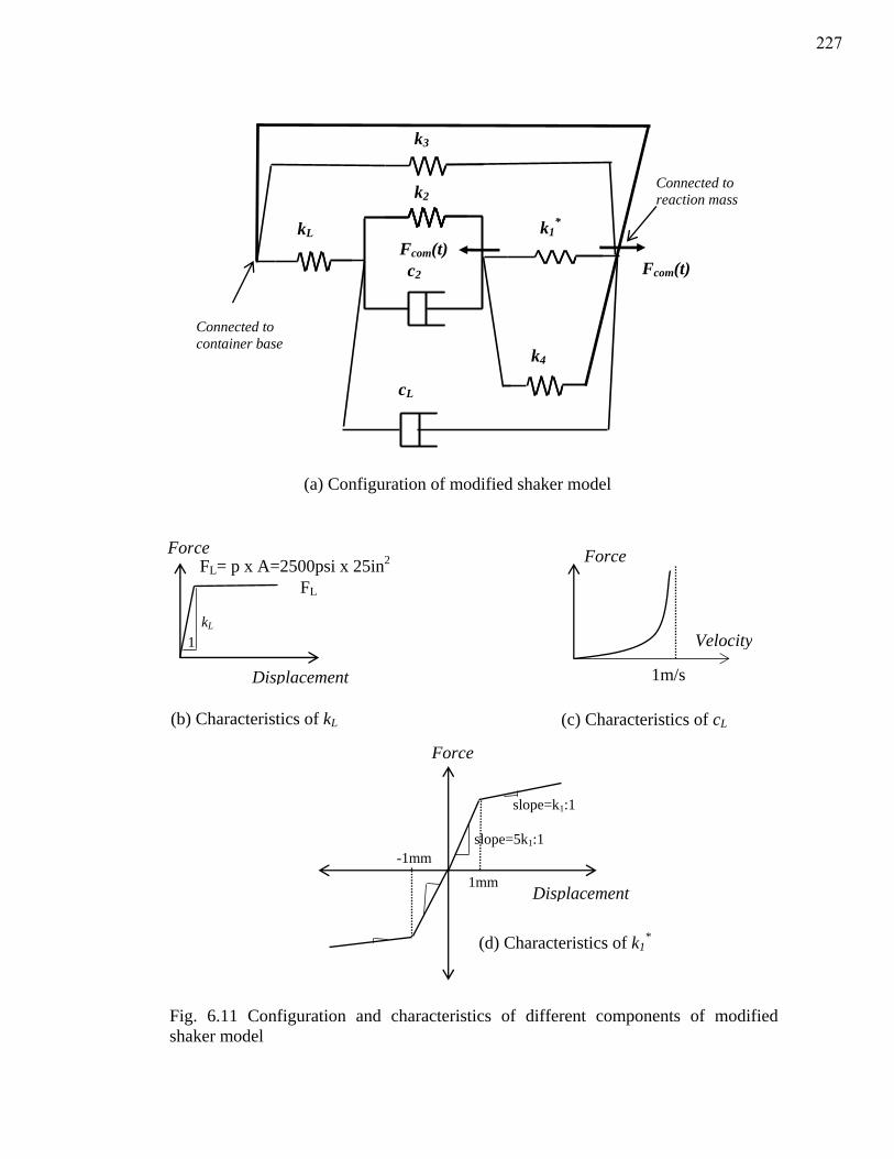
Fig. 6.11 Configuration and characteristics of different components of modified
shaker model
kL
k3
k2
cL
k1*
k4
c2 Fcom(t) Fcom(t)
Connected to reaction mass
Connected to container base
(a) Configuration of modified shaker model
Force
Velocity
1m/s
(c) Characteristics of cL (b) Characteristics of kL
FL= p x A=2500psi x 25in2Force
Displacement
FL
1 kL
Force
Displacement 1mm
slope=5k1:1
slope=k1:1
-1mm
(d) Characteristics of k1*
227
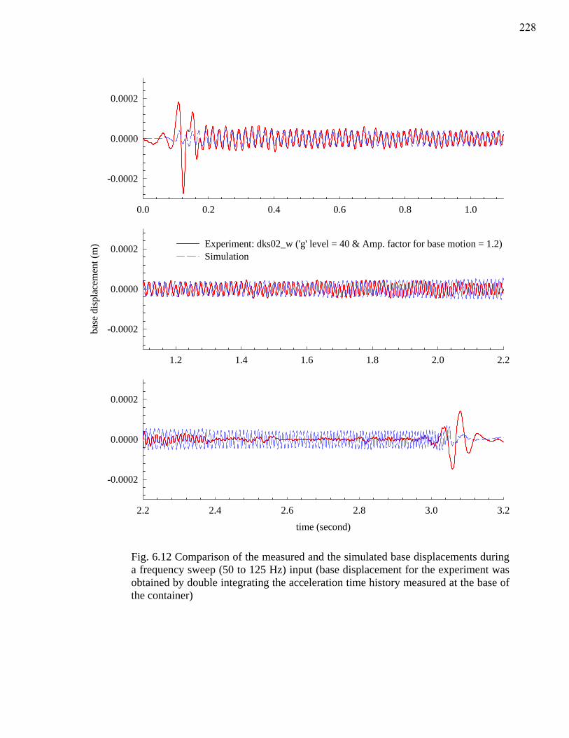
0.0 0.2 0.4 0.6 0.8 1.0
-0.0002
0.0000
0.0002
1.2 1.4 1.6 1.8 2.0 2.2
base
dis
plac
emen
t (m
)
-0.0002
0.0000
0.0002 Experiment: dks02_w ('g' level = 40 & Amp. factor for base motion = 1.2)Simulation
time (second)
2.2 2.4 2.6 2.8 3.0 3.2
-0.0002
0.0000
0.0002
Fig. 6.12 Comparison of the measured and the simulated base displacements during a frequency sweep (50 to 125 Hz) input (base displacement for the experiment was obtained by double integrating the acceleration time history measured at the base of the container)
228
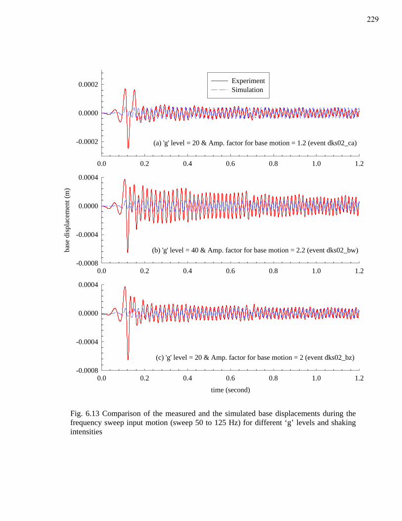
(a) 'g' level = 20 & Amp. factor for base motion = 1.2 (event dks02_ca)
0.0 0.2 0.4 0.6 0.8 1.0 1.2
-0.0002
0.0000
0.0002
(b) 'g' level = 40 & Amp. factor for base motion = 2.2 (event dks02_bw)
0.0 0.2 0.4 0.6 0.8 1.0 1.2
base
dis
plac
emen
t (m
)
-0.0008
-0.0004
0.0000
0.0004
ExperimentSimulation
(c) 'g' level = 20 & Amp. factor for base motion = 2 (event dks02_bz)
time (second)
0.0 0.2 0.4 0.6 0.8 1.0 1.2-0.0008
-0.0004
0.0000
0.0004
Fig. 6.13 Comparison of the measured and the simulated base displacements during the frequency sweep input motion (sweep 50 to 125 Hz) for different ‘g’ levels and shaking intensities
229
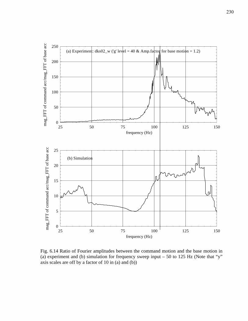
frequency (Hz)25 50 75 100 125 150m
ag_F
FT o
f com
man
d ac
c/m
ag_F
FT o
f bas
e ac
c
0
50
100
150
200
250
(b) Simulation
frequency (Hz)25 50 75 100 125 150m
ag_F
FT o
f com
man
d ac
c/m
ag_F
FT o
f bas
e ac
c
0
5
10
15
20
25
(a) Experiment: dks02_w ('g' level = 40 & Amp.factor for base motion = 1.2)
Fig. 6.14 Ratio of Fourier amplitudes between the command motion and the base motion in (a) experiment and (b) simulation for frequency sweep input – 50 to 125 Hz (Note that “y” axis scales are off by a factor of 10 in (a) and (b))
230
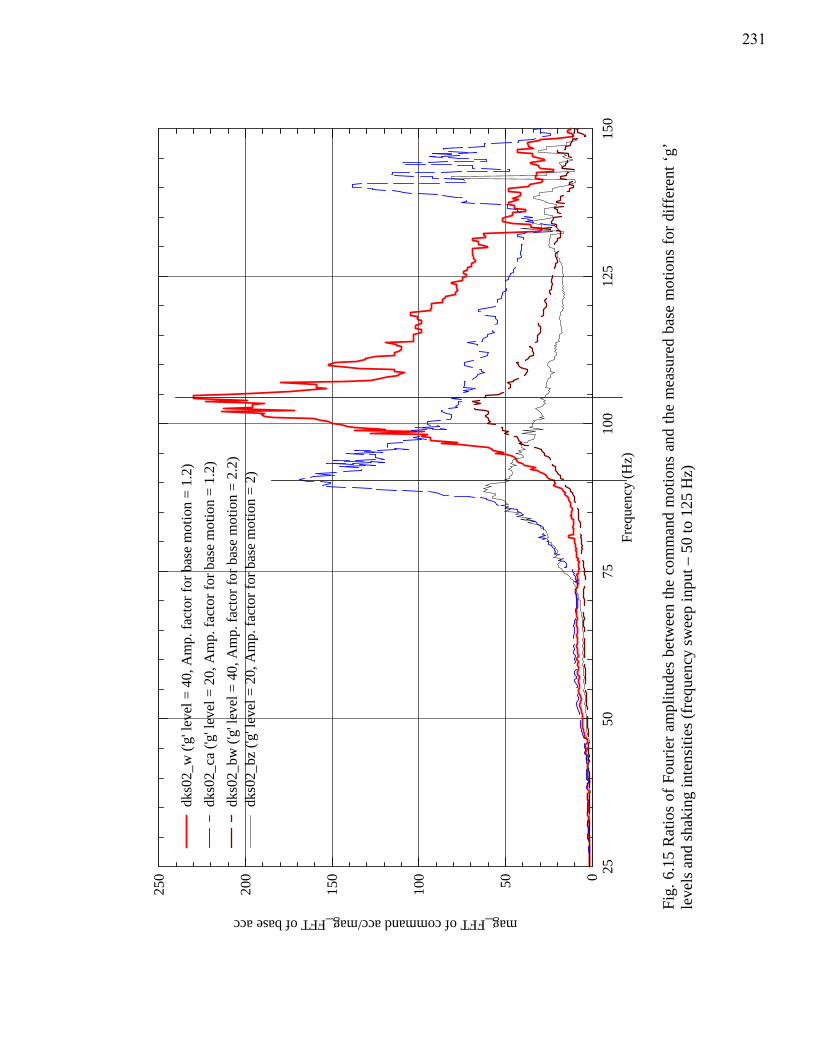
Freq
uenc
y (H
z)25
5075
100
125
150
mag_FFT of command acc/mag_FFT of base acc
050100
150
200
250
dks0
2_w
('g'
leve
l = 4
0, A
mp.
fact
or fo
r bas
e m
otio
n =
1.2)
dks0
2_ca
('g'
leve
l = 2
0, A
mp.
fact
or fo
r bas
e m
otio
n =
1.2)
dks0
2_bw
('g'
leve
l = 4
0, A
mp.
fact
or fo
r bas
e m
otio
n =
2.2)
dks0
2_bz
('g'
leve
l = 2
0, A
mp.
fact
or fo
r bas
e m
otio
n =
2)
Fig.
6.1
5 R
atio
s of
Fou
rier a
mpl
itude
s be
twee
n th
e co
mm
and
mot
ions
and
the
mea
sure
d ba
se m
otio
ns fo
r diff
eren
t ‘g’
le
vels
and
shak
ing
inte
nsiti
es (f
requ
ency
swee
p in
put –
50
to 1
25 H
z)
231
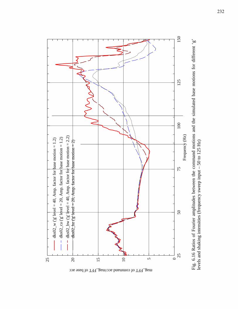
Freq
uenc
y (H
z)25
5075
100
125
150
mag_FFT of command acc/mag_FFT of base acc
0510152025dk
s02_
w ('
g' le
vel =
40,
Am
p. fa
ctor
for b
ase
mot
ion
= 1.
2)dk
s02_
ca ('
g' le
vel =
20,
Am
p. fa
ctor
for b
ase
mot
ion
= 1.
2)dk
s02_
bw ('
g' le
vel =
40,
Am
p. fa
ctor
for b
ase
mot
ion
= 2.
2)dk
s02_
bz ('
g' le
vel =
20,
Am
p. fa
ctor
for b
ase
mot
ion
= 2)
Fig.
6.1
6 R
atio
s of
Fou
rier
ampl
itude
s be
twee
n th
e co
mm
and
mot
ions
and
the
sim
ulat
ed b
ase
mot
ions
for
diff
eren
t ‘g’
le
vels
and
shak
ing
inte
nsiti
es (f
requ
ency
swee
p in
put –
50
to 1
25 H
z)
232
Chapter 7
Summary and Conclusions, and Future work
7.1 Summary and Conclusions
This dissertation consists of the following four components: (1) A collaborative
research project involving centrifuge testing and numerical simulation of a soil-pile-
bridge system (2) A critical study to advance understanding the effects of using different
input motion boundary conditions on the sensitivity of numerical simulation results to
errors in material properties of a specimen tested on a shaking table (3) Numerical
simulations of a soil model tested on the centrifuge experiment accounting for soil-
container-shaker interaction, and (4) A first attempt to develop a numerical model of the
UC Davis servo-hydraulic centrifuge actuation system with a goal of predicting shaking
table response.
7.1.1 Collaborative research: Centrifuge testing of soil-pile-bridge systems
The centrifuge experiments on soil-pile-bridge systems presented in this
dissertation were a part of a multi-university collaborative research project utilizing
NEES with goal of investigating the effects of Soil-Foundation-Structure-Interaction
(SFSI) while demonstrating NEES research collaboration (Wood et al. 2004). Much had
been learned from this collaborative research with respect to means for effective research
collaboration and investigating SFSI effects by integrating experimental and analytical
tools.
233
7.1.1.1 Research collaborations
Sixteen principal and co-principal investigators from ten universities were
involved in this collaborative research. The experimental component of the research
involved 1-g shake table experiment at the University of Nevada at Reno (Johnson et al.
2006), field tests using the large mobile shakers at the University of Texas at Austin
(Black 2005), centrifuge tests at the University of California at Davis (Ilankatharan et al.
2005), and quasi-static structural component testing at Purdue University (Makido 2007).
The team of researchers also included numerical analysts from the University of
Washington (Shin 2007 and Ranf 2007), the University of California at Davis (Jie 2007),
and the University of California at Berkeley (Dryden 2008), as well as a team of
researchers at Kansas University to coordinate and sharing of data, and an education and
outreach team at San Jose State University.
Unlike most scientific research that has been led by only one to few collaborators
working on the same project and at the same test facility, multi-institution, multi-
investigator collaborative research requires particular attention to issues related to the
involvement, coordination, and cooperation of a large number of led researchers and their
support staff. Therefore, effective communication tools to facilitate information exchange
and decision making are essential to effectively conduct a large-scale collaborative
research. Periodic video and audio conference calls in addition to several face-to-face
meetings were held to facilitate information exchange and decision making. These were
in addition to extensive use of group emails and one-on-one interactions through emails
and phone calls. Arguably, a valuable research experience was obtained about open
234
exchange of ideas and effective dissemination of knowledge, from working on this
geographically distributed and diverse research environment.
Furthermore, the design of test elements to account for different test boundary
conditions and test scaling laws for structural modeling and geotechnical modeling was
challenging. The design process required cross-disciplinary interaction between
geotechnical and structural engineering. This cross disciplinary interaction may lead to
more holistic soil-structure system designs. The negotiation of the designs of test
elements to the satisfaction of the cross-disciplinary research team was an extremely
valuable learning experience.
7.1.1.2 Centrifuge experiments
The centrifuge experiments presented in this dissertation involved 1/52 scale
models of two-pile bents, single piles and a two-span segment of bridge with 20 different
superstructure configurations tested under varying earthquake characteristics (level of
shaking, frequency content, and wave from). These experiments produced unique data
sets that span the disciplines of geotechnical and structural engineering. Some of these
data complement the data obtained from other experiments. The data from the centrifuge
experiments was compared and combined with the data obtained from other experiments
to provide integrated analytical models for SFSI problems of soil-pile-bridge systems.
Comparisons with field tests
The MIL02 test series, in which the bridge bents were oriented to the different
directions of base shaking, was designed to facilitate comparisons with the field tests
performed at the University of Texas at Austin, in which the vibration source (T-Rex)
was moved to different locations relative to the model bridge bent. As the field shakers
235
which have maximum force outputs in a higher frequency range (http://nees.utexas.edu),
the natural frequencies of the field test specimens were altered by a factor of 18 (by
reducing the bent-cap masses) to increase the response to the excitation. These
differences in the range of frequencies of response of test specimens in both experiments
posed difficulties in making direct comparisons between experimental results. However,
both experiments provided unique data about the response of prototype bridge structure.
These unique data sets were used to calibrate the simulation methods for seismic soil-
foundation-structure interaction problems (Shin 2007 and Jie 2007).
Comparisons with 1-g shake table experiment
Comparisons of experimental results and the resolution of issues associated with
comparing physical models of the two-span segment of the bridge model tested at the
geotechnical centrifuge and the 1-g shake table facilities were presented in Chapter 3 of
this dissertation. For intermediate levels of shaking, the agreement between deck
response in centrifuge and 1 g shake table experiments suggests that the bridge deck
response can be reasonably modeled using fixed base columns attached to a 1 g shake
table if the 1 g shake table motion corresponds to the free field soil motion at the
equivalent depth of fixity (Chai, 2002). A difference in prototype bent spacing between
the centrifuge and 1-g shaking table models in addition to the interaction between the 1 g
shake table bridge model with the 1 g shaking table/actuation system caused some
discrepancies between centrifuge results and 1 g shaking table results. There were also
differences in spectral ratios (ratio of spectral acceleration of the deck to spectral
acceleration at the depth of fixity) that may be attributable to different energy dissipation
mechanisms in centrifuge and 1 g shake table experiments: soil particle-particle friction
236
and sliding, particle crushing, friction at soil-pile interface, radiation damping provided
by the piles in the soil, pile/column yielding and radiation damping in shake table system.
A significant amount of energy dissipation that occurred in the centrifuge test during the
medium-level shaking event was not present in shake table test. However, shake table
bridge model dissipated more energy during large-level of shaking due to yielding of the
reinforced concrete column. Hence, the direct comparison of results from different types
of experiments is valuable because it can clearly expose the flaws that we might
otherwise ignore.
Comparison of the system (three-bent) response to the individual bent response
The bridge deck in the centrifuge model of the two-span segment of the bridge
consisted of a light-weight aluminum plate bolted to the bridge bents. This afforded the
opportunity to first test each the three bents simultaneously while they were unconnected
and then to test them as a three-bent system. The comparisons of bent responses,
presented in Chapter 3 for a relatively weak input motion (measured base motion 0.08 g
in prototype scale), showed that the system response was quite different from individual
bent response. If the columns or the soil around the piles were to yield significantly this
could result in additional complex interactions. Theoretically, these interactions could be
predicted using numerical methods such as finite elements; however the methods for
analyzing soil-foundation-bridge systems have not been subject to verification exercises.
While experiments on bridge components will continue to be valuable, tests of
soil-foundation-bridge systems lead to more complete understanding of system
performance, provide unique data sets to validate numerical methods to predict bridge
system response, and promote cross-disciplinary education of researchers. Continued
237
multi-institution, multi-disciplinary research on systems could lead to a new paradigm for
design in which foundations and superstructures are designed to have stiffness, capacity,
and energy dissipation characteristics that are compatible and complementary with the
goal of optimizing system performance.
7.1.1.3 Centrifuge test data archives
One of the goals of this collaborative research was to develop curated data
repositories of the experimental and simulation data of SFSI problems of the prototype
bridge structure. In this context, all centrifuge test data and metadata was archived and
curated in NEEScentral data repository, and was used to demonstrate the usage of end-to-
end flow of data (Van Den Einde at al. 2007) using a data viewer (N3DV) developed by
the researchers at UC Davis (http://neesforge.nees.org). The data archives are publically
available at the NEEScentral website (http://central.nees.org).
7.1.1.4 Numerical simulations of the centrifuge experiments
The numerical simulations of all the centrifuge experiments were performed by
the collaborators from the University of Washington (Shin 2007). These simulations
employed Dynamic Beam-on-Nonlinear-Winkler Foundation (BNWF) models, using p-y,
t-z, and q-z interface springs (Boulanger et al. 1999) coupled with a 1-D shear beam soil
column, to model seismic soil-pile-structure interaction. Some of these simulations were
performed prior to the experiments and during the experiments. Results from these pre-
test and real-time simulations were valuable in designing test specimens and loading
protocols (i.e. selection of earthquake characteristics).
Some of the comparisons between the results from the post-test simulations and
experiments were presented in Chapter 2. These comparisons suggest that overall the
238
simulations reasonably predicted the superstructure motions and the maximum pile
bending moments. However, significant discrepancies (especially those near the ground
surface) between the predicted and measured soil motions were observed from these
comparisons. Shin (2007) also performed sensitivity analyses to study the sensitivity of
simulation results to uncertainties in modeling parameters. These sensitivity analyses
considered simulations of a single pile and a two-pile bent. For the structural models and
ground motion characteristics considered in these sensitivity studies, it was concluded
that the simulated superstructure motions and maximum pile bending moments were not
very sensitive to change in soil motions.
Effect of modeling boundary conditions on the sensitivity of predicted site
response
As mentioned earlier, the numerical simulations presented above employed a 1-D
shear beam shear-beam type finite element model to simulate soil site response. Effects
of model container on the soil site response were not explicitly modeled in these
simulations. The effect of mass of the container on the inertia forces was accounted (by
increasing unit weight of soil by 30%); however, flexibility of the container and the
stiffness of the vertical bearing supports at the base of the container were not modeled in
these simulations. In addition, these simulations adapted the measured motion at the base
of the container a prescribed motion for dynamic excitation. It is evident from the
presented comparisons in this dissertation that, in some cases, the predicted soil motions
(especially those near the ground surface) from the above simulations were significantly
different from experimental results. Understanding the discrepancies of these predicted
site response results motivated the analyses presented in the second part of this
239
dissertation. In this context, it was hypothesized that the “sensitivity of simulation results
to uncertainties in modeling parameters depends on how the boundary conditions are
incorporated in the simulations”. The second part of this dissertation is intended to prove
this hypothesis.
7.1.2 Modeling input motion boundary conditions for simulations of geotechnical
shaking table experiments
Numerical simulations of a hypothetical centrifuge shaking table experiment
involving a 1D soil column were performed in Chapter 4 to illustrate effects of using
different input motion boundary conditions on the sensitivity of numerical simulation
results to errors in material properties of a specimen. A novel method for handling the
boundary developed in this dissertation is the flexible-actuator-prescribed-force boundary
condition; by this method seismic input is specified by a force across a relatively stiff
spring in series with the actuator that drives the shaking table; hence, the boundary
between the test specimen and the shaking table is an absorbing-base boundary across
which energy may be transferred. In the prescribed-displacement boundary condition (the
more conventional method for introducing the excitation), the measured shaking table
motion in the experiment is used as a prescribed displacement in the simulation.
In both the simulations using the linear elastic and the elasto-plastic PDMY soil
material models, if the shear modulus of the soil material is perfectly modeled then the
results are independent of the input motion boundary conditions. Conversely, the
predicted surface response is dependent on the input motion boundary conditions when
the shear modulus is imperfectly modeled in the simulations. As expected, it is shown
that the ratio of Fourier amplitudes between the surface motion and the base motion (i.e
240
surface transfer function) is independent of the input motion boundary conditions when a
linear elastic soil material with an imperfect shear modulus is employed in the analysis.
However, the ratio of Fourier amplitude between the surface motion and the base motion
is dependent on the input motion boundary conditions when a nonlinear soil material with
an imperfect shear modulus is used in the analysis. In this case, greater discrepancies are
observed near frequencies at which peaks of ratio of Fourier amplitudes occur. The ratio
of Fourier amplitudes between the base motion and the command motion (i.e. base
transfer function) is dependent on the input motion boundary conditions when the shear
modulus of the soil material (both in linear elastic and PDMY material) is imperfectly
modeled in the simulations. This is because the dips (valleys) in the base transfer function
associated the energy absorption of the overlying soil deposit occur at the natural periods
of the soil, but the calculated amplification (peaks) in the surface transfer function
depends on the assumed natural periods which depend on the assumed shear modulus in
the simulations. If an absorbing-base boundary is assumed then the changes in frequency
of dips is compensated for by the changes in frequency of amplification. These changes
in base response cannot be evaluated using the prescribed-displacement input motion
boundary condition.
Furthermore, the flexible-actuator-prescribed-force approach which employs an
absorbing-base boundary generally yields well behaved sensitivities for results in a wide
range of simulation conditions. The prescribed-displacement approach, however, may
produce chaotic results in the sense that small errors in the simulation lead to large errors
in the results. Therefore, when performing the numerical simulations of a shaking table
experiment, modeling input excitation using the flexible-actuator-prescribed-force
241
boundary condition may be preferable to the prescribed-displacement boundary
condition.
The most general conclusion of this study is that the sensitivity of numerical
simulation results to uncertainties in modeling parameters depends on how the input
motion boundary conditions are accounted for and the dynamic interactions among the
various components of the dynamic system. This raises a fundamental question: How can
we assess the significance of a discrepancy between a numerical simulation and an
experimental result? A large error in response may be caused by a small error in input
parameter if, for example, a rigid boundary condition is assumed. This study shows that,
for shaking table tests, the significance of errors in the numerical simulations cannot be
rigorously assessed without accounting for dynamic interaction between the test
specimen and the actuation system.
7.1.3 Numerical simulations of the soil model accounting for soil-container-shaker
interaction
Numerical modeling of complex dynamic interaction of a soil-model container-
centrifuge-shaker system was presented in Chapter 5 of this dissertation. This modeling
incorporated mass and flexibility of the container (a flexible shear beam container), the
effect of shear rods at both ends of the container, stiffness of the vertical bearing supports
at the base of the container, flexibility of the actuator, and the effect of reaction mass. A
simplistic approximation of the actuator and control system using springs and dashpots
was used to include first-order effects of actuator flexibility on the interaction between
the specimen and the shaking table.
242
To improve understanding of interactions among soil model, container, and
shaker system and to evaluate how the sensitivity of simulation results depends on
boundary conditions in experiment and simulation, the boundary conditions were treated
with three different levels of detail: (a) 1-D shear beam simulations of soil column (b) 2-
D simulations of soil and container, and (c) 2-D simulations of soil, container, and
shaker. Site response simulations using the above numerical models were performed and
results were compared with the site response results measured in the centrifuge test series
MIL03.
As opposed to the 1-D shear beam simulations of soil, the inclusion of the
container in the simulations resulted in more accurate simulation of the experiment. In
addition, the rocking behavior of the container was well captured when the compliance of
the vertical bearing supports at the base of the container was included in the analysis.
Sensitivity studies were performed to propagate the uncertainties in modeling shear
modulus of the soil on the predicted site response results for models at the three levels of
detail. Results from sensitivity studies showed that the sensitivity of computational
simulation output (soil site response) to changes in input parameters (shear modulus of
soil) depends on how boundary conditions were modeled in the simulation; to provide an
unbiased validation of a numerical model, it is important evaluate the effects of boundary
conditions on the sensitivity of simulation results. Similar to the results presented in
chapter 4 for the simulations with the hypothetical centrifuge experiment, it was again
shown that the sensitivity of predicted site response results heavily depends on the input
motion boundary conditions. In addition, the 2-D simulations of soil, container, and
shaker, which employed the flexible-actuator-prescribed-force input motion boundary
243

condition for input excitation, generally yield well behaved sensitivities for predicted site
response results.
The numerical models of the soil-container-shaker system are archived and
publically available for other to use in NEEScentral data repository
(http://central.nees.org). These simulations of the soil-container-shaker system consider a
uniform dry-dense sand soil model, a flexible shear beam, and the horizontal shaker of
the UC Davis centrifuge facility. Others could access these numerical models, modify
the geometry of the FE mesh and the definition of constitutive models and input
parameters of the soil model, and update the FE mesh of the soil-container-shaker
system, to simulate different experiments. Additional details on the simulation archives
are given in Chapter 5 and Appendix A of this dissertation.
7.1.4 Numerical model of a servo-hydraulic centrifuge actuation system to predict
shaking table response
Modeling the input motion boundary condition using the flexible-actuator-
prescribed-force approach requires a realistic representation of experimental boundary
conditions and the detailed modeling of various components of the centrifuge-shaker
system to include the effects of dynamic interaction between the test specimen and the
servo-hydraulic actuation system on the simulation results. Another benefit of accurate
modeling of the centrifuge-shaker system is the accurate prediction of base motions in the
simulations. Further, this numerical model could be used to predict base motions during
input motion tuning exercises prior to the actual experiment.
In the absence OpensSees material models and elements to model various
components of the servo-hydraulic actuation system, a simplistic approximation using
244
springs and dashpots was used to model the actuator, servo-valve and the control system
in the numerical model of the UC Davis centrifuge actuation system. Generally, for the
soil model (dry dense Nevada sand) and the frequency sweep input (50 to 125 Hz)
considered in the simulations, the above shaker model reasonably reproduced some
features (for example, steady state components of base displacements) of the base
response observed in the experiment. However, the higher frequency components of the
base displacements and the magnitudes of the base transfer functions (i.e., ratios of
Fourier amplitude between the base motion and command motion) were poorly predicted
in the simulations. Also, while the results were not presented in this dissertation, the
simulations using the command motions with significantly higher frequency contents
resulted in poor predictions of the base displacements and the base transfer functions.
In general, the degree of distortion between the input command motion and the
measured motion at the shaking table depends on numerous factors such as the
characteristics of the soil model, compressibility of oil column in the actuator, non-linear
flow characteristics in the actuator, servo-valve time delay, configuration of control loops
etc. Geotechnical centrifuge experiments often involve highly non-linear test specimens
where the payload mass is a significant fraction of the system mass and the larger
amplitude earthquake simulations where the actuator characteristics are themselves non-
linear. In addition, in the centrifuge experiments frequencies are scaled by the factor of
‘g’ level. The resonant frequencies of higher vibration modes of different components of
the actuation system and the higher frequency responses of the actuator, the servo-valve
and the control system would affect the characteristics (magnitude, frequency content,
and wave form) of the dynamic signal measured at the shaking table. Therefore, to
245
capture the salient features of the non-linear actuator and servo-valve and to compensate
for the effects of poles and zeros that develop in the feed-back control system on the
shaking table response, it is concluded that more sophisticated analytical models of the
actuator, servo-valve, and controller are required.
7.2 Areas for future research
Recent research has begun to further understand the seismic response of soil-
foundation-bridge systems and to verify and validate computational simulations for
seismic response of bridge systems. Some ideas for future research on seismic response
of soil-foundation-bridge systems are listed below.
Experimental research on soil-foundation-bridge systems which involves poor soil
conditions need to be conducted (to investigate the effects of liquefaction and
lateral spreading for example). Data from these experiments could then be used to
calibrate the integrated numerical models of complete bridge systems (i.e., soil-
foundation systems with realistic superstructure characteristics) which involve
complex mechanisms of behavior (response to kinematic loads from liquefaction
induced lateral spreading for example).
Additional experimental data is required to evaluate the effects of inelastic
deformations and energy dissipation characteristics (formation of an in-ground
plastic hinge for example) of the foundation on the system response of the bridge.
The experiments presented in this dissertation involved bridge systems with a
larger diameter drilled shaft foundation configuration. Additional experimental
data is required to fully understand the seismic response of soil-foundation-bridge
246
systems which involve other foundation configurations (for example, pile groups,
shallow foundations, etc.)
The effect of abutment structures on the performance of bridge system needs to be
completely evaluated; which requires experimental research on soil-foundation-
deck-abutment systems. Results from these studies could then be used to calibrate
integrated numerical models of complete bridge systems and to develop improved
design guidelines for seismic applications.
The analyses presented in the second part of this dissertation provided insight into
the importance of proper treatment of experimental boundary conditions on the
sensitivity studies of numerical simulations. The effects of dynamic interaction between
the soil model and the centrifuge shaker system on the simulations of the centrifuge
experiments were incorporated up to a certain extent, yet much research need to be
performed to fully understand effects of dynamic interaction between a test specimen and
the centrifuge shaker system in various scenarios. Some ideas for future research on this
problem are listed below.
The analyses presented in the second part of the dissertation focused solely on the
site response simulations and investigated the effects of soil-container-shaker
interaction on the site response results. Numerical simulations of the complete
experimental system (i.e., includes bridge model, soil, container, and shaker),
with a realistic representation of experimental boundary conditions and the
detailed modeling of dynamic interactions between the test specimen and the
centrifuge shaker system (i.e., interactions between bridge model-soil-container-
shaker), are to be performed to fully understand the sensitivity of simulated bridge
247
model response (such as super structure response, pile bending moment, etc) to
uncertainties in modeling parameters.
Dynamic interaction between a test specimen and the servo-hydraulic actuation
system depends on many factors such as characteristics of the test specimen,
compliance of reaction mass, compressibility of oil column in the actuator
chamber, non-linear flow characteristics in the actuator, servo valve time delay,
configuration and characteristics of control loops, etc. Therefore to fully
incorporate the effects of the test specimen-actuation system interaction on the
simulation models, sophisticated models of actuator, servovalve, and controller
are required. Development of these analytical models, especially for the
geotechnical centrifuge applications, is a topic for future research.
Geotechnical centrifuge experiments often involve relatively heavy and highly
nonlinear test specimens (e.g., a massive volume of liquefying sand). Additional
work is required to understand the interaction of highly nonlinear massive test
specimens with servo-hydraulic centrifuge actuation systems that are driven at
their performance limits (in their nonlinear range).
248
References
Abdoun, T., Dobry, R., O’Rourke, T. D., and Goh, S. H. (2003). ‘‘Pile response to lateral
spreads: Centrifuge modeling.’’ J. Geotech. Geoenviron. Eng., ASCE. 129(10), 869–
878.
Agarwal, P., Black, J. S., Wood, S. L., Kurtulus, A., Menq, F., Rathje, E. M., and Stokoe,
K. H. (2006). “Dynamic field tests of small-scale bridge bents supported on drilled
shafts”, 8th National Conf. Earthquake Engineering, San Fransisco, Calif., April
2006.
Armstrong, R. J., Boulanger, R. W., Gulerce, U., Kutter, B. L., and Wilson, D. W.
(2008). "Centrifuge modeling of pile pinning effects." Geotechnical Earthquake
Engineering and Soil Dynamics IV, D. Zeng, M. Manzari, and D. Hiltunen, eds.,
Geotechnical Special Publication No. 181, ASCE, NY.
Arulanandan, K. and Scott, R. F., (1993). Project VELACS; control test results, Journal
of geotechnical engineering, 119(8), 1276-1292.
Arulnathan, R., Boulanger, R. W., Kutter, B. L., and Sluis, W. K. (2000). “New tool for
shear wave velocity measurements in model tests.” Geotechnical testing journal,
23(4): 444-453.
249
Black, J. S., (2005). “Design and construction of small-scale bridge bents on drilled shaft
foundations,” M.S. Thesis, Department of Civil Engineering, University of Texas,
Austin.
Boulanger, R. W., Curras, C. J., Kutter, B. L., Wilson, D. W., and Abghari, A. (1999),
“Seismic Soil-Pile Structure Interaction Experiments and Analysis” Journal of
Geotechnical and Geoenvironmental Engr., ASCE, Vol. 125, No. 9, pp. 750-759.
Brandenberg, S. J. (2005). "Behavior of pile foundations in liquefied and lateral
spreading ground" Ph.D. dissertation, University of California, Davis.
Chai, Y. H. (2002). “Flexural strength and ductility of extended pile-shafts. I: Analytical
model,” Journal of Struct. Eng., 128(5): 586-594.
Chang, D., R.W. Boulanger, B.L. Kutter, and S.J. Brandenberg. (2005): "Experimental
Observations of Inertial and Lateral Spreading Loads on Pile Groups during
Earthquakes” ASCE GeoFrontiers 2005, (Paul W. Mayne, Ellen Rathje, Jason
DeJong, Amy Rechenmacher, Jerry Yamamuro, Sunil Sharma, Clinton Willson eds.),
Austin Texas. January.
Conte, J. P., and Trombetti, T. L., (2000). “Linear Dynamic Modeling of a Uni-Axial
Servo-Hydraulic Shaking Table System”, Earthquake Engineering and Structural
Dynamics, Vol. 29, No. 9, pp. 1375-1404.
Algie, T. B., Deng, L., Erduran, E., Kutter, B. L., and Kunnath, S. (2008), “Centrifuge
modeling of innovative foundation systems to optimize seismic behavior of bridge
250
structures” Proceedings, 14th World Conference on Earthquake Engineering, Beijing,
China, October 12-17.
Dryden, M., and Fenves, G. L., (2008). “Validation of numerical simulations of a two-
span reinforced concrete bridge” Proceedings, 14th World Conference on Earthquake
Engineering, Paper 0073, Beijing, China, October 12-17.
Elgamal, A., Yang, Z., Lai, T., Kutter, B.L., and Wilson, D.W., (2005). Dynamic
Response of Saturated Dense Sand in Laminated Centrifuge Container, J. Geotech.
Geoenviron. Eng., ASCE, 131(5) pp. 598-609.
Fiegel, G.L., M.Hudson, I.M. Idriss, B.L. Kutter, and X. Zeng, (1994) "Effect of Model
Containers on Dynamic Soil Response", Centrifuge 94, Leung, Lee and Tan (eds.),
Balkema, Rotterdam, pp. 145-150.
Gazetas, G. and Mylonakis, G. (1998). “Seismic Soil-Structure Interaction: New
Evidence and Emerging Issues”. Geotechnical Earthquake Engineering and Soil
Dynamics III, ASCE, Editors: P. Dakoulas, M. Yegian and R. D. Holtz, ASCE
Geotechnical Special Publication No.75, pp 1119-1174.
Ilankatharan, M., and Kutter, B. L. (2008). “Modeling Input Motion Boundary
Conditions for Simulations of Geotechnical Shaking Table Tests.” Earthquake
Spectra, Earthquake Engineering Research Institute (under review).
Ilankatharan, M., and Kutter, B. L., (2008). Numerical Simulation of a Soil Model-Model
Container-Centrifuge Shaking Table System, Geotechnical Earthquake Engineering
251
and Soil Dynamics IV, D. Zeng, M. Manzari, and D. Hiltunen, eds., Geotechnical
Special Publication No. 181, ASCE, NY.
Ilankatharan, M., Kutter, B.L., H. Shin, P. Arduino, S.L. Kramer, N. Johnson, and T.
Sasaki. (2006). “Comparison of Centrifuge and 1g Shaking Table Models of a Pile
Supported Bridge Structure,” Proceedings of the 6th International Conference on
Physical Modeling in Geotechnics, Hong Kong, Vol. 2: 1313-1318, August, 2006.
Ilankatharan, M., Sasaki, T., Shin, H., Kutter, B. L., Arduino, P., and Kramer, S. L.,
(2005). “A demonstration of NEES system for studying soil-foundation-structure
interaction,” Centrifuge data report for MIL01, Rep. No. UCD/CGMDR-05/05, Ctr.
for Geotech. Modeling , Dept. of Civ. and Envir. Engrg., University of California,
Davis, Calif.
Jie, G. (2007). “High Performance Computational Geomechanics and Applications to the
Soil–Foundation–Structure Interaction Problems”, Ph.D. dissertation, University of
California, Davis.
Johnson, N., Ranf, R., Saiidi, M., Sanders, D., and Eberhard, M. (2006). “Shake-Table
Studies of a Two-Span, Reinforced Concrete Bridge,” Proceedings, Eighth National
Conference on Earthquake Engineering, April 2006.
Johnson, N., Saiidi, M., and Sanders, D. (2006). “Large-scale experimental and analytical
seismic studies of a two-span reinforced concrete bridge system.” Civil Engineering
Dept., Univ. of Nevada, Reno,Nev.
252

Jung, R. Y., and Shing, P. B., (2006). Performance evaluation of a real-time
pseudodynamic test system, Earthquake Engineering and Structural Dynamics, Vol.
35, No. 7, pp. 789-810.
Kurtuluş, A., Lee, J.J., and Stokoe, K.H., 2005. “Summary report, site characteristics of
Capital Aggregates test site,” Department of Civil Engineering, University of Texas,
Austin, 47 pp.
Kutter, B.L., (1995). Recent Advances in Centrifuge Modeling of Seismic Shaking,
State-of-the-Art Paper, Proceedings, Third International Conference on Recent
Advances in Geotechnical Earthquake Engineering and Soil Dynamics, St. Louis,
MO, Vol.2, pp. 927-942.
Kutter, B.L. (1992). "Dynamic centrifuge modeling of geotechnical structures."
Transportation Research Record 1336, TRB, National Research Council, National
Academy Press, Washington, D.C., pp. 24-30.
Kutter, B.L., and Wilson, D.W. (2006). "Physical Modeling of Dynamic Behavior of
Soil-Foundation-Superstructure Systems," Invited paper, International Journal of
Physical Modelling in Geotechnics. Vol. 6 No. 1, pp. 1-12.
Kutter, B.L., Idriss, I.M., Kohnke, T., Lakeland, J., Li, X.S., Sluis, W., Zeng, X.,
Tauscher, R., Goto, Y., and Kubodera, I. (1994). "Design of a large earthquake
simulator at UC Davis." Proceedings, Centrifuge 94, Leung, Lee, and Tan, Eds.,
Balkema, Rotterdam, pp. 169-175.
253
Madabhushi, S.P.G., Bulter, G., and Schofield, A.N. (1998) "Design of an equivalent
shear beam (ESB) container for use on the US Army Centrifuge", Centrifuge 98,
Kimura, Kusakabe and Takemura (eds.), Balkema, Rotterdam, pp. 117-122.
Makido, A. (2007). “Behavior of spirally reinforced concrete columns under load
reversals.” Ph.D. thesis, Purdue Univ., West Lafayette, La.
Mazzoni, S., McKenna, F., Scott, M.H., and Fenves, G., (2006). The OpenSees Command
Language Manual: version 1.7.3, Pacific Earthquake Engineering Center, Univ. of
Calif., Berkeley. ⟨http://opensees.berkeley.edu⟩.
Mejia, L.H., and Dawson, E.M., (2006). Earthquake Deconvolution for FLAC,
Proceedings, Fourth International FLAC Symposium on Numerical Modeling in
Geomechanics, Madrid, Spain.
Narayanan, K.R. (1999). "Modeling the seismic response of stratified soil," Masters of
Science Thesis, University of California, Davis.
Priestly, M. J. N., Seible, F., and Calvi, G. M. (1998). “Seismic design and retrofit of
bridge,” Wiley-Interscience, New York.
Ranf, R. T. (2007). “Model selection for performance-based earthquake engineering of
bridges.” Ph.D. thesis, Univ. of Washington, Seattle, Wash.
Reese, L., Cox, W., and Koop, F. (1974). “Analysis of laterally loaded piles in sand”,
Proceedings of the VI Annual Offshore Technology Conference, Houston, Texas
(OCT 2080), 473-485.
254
Schofield, A. N. (1981), “Dynamic and earthquake centrifuge modeling”,Proceedings of
the International Conference on Recent Advances in Geotech. Earthquake Eng. and
Soil Dynamics, St. Louis, Missouri, 1981, vol. III, pp. 1081–1099.
Shin, H. (2007), “Numerical modeling of a bridge system and its applications for
performance- based earthquake engineering”, Ph.D. dissertation, University of
Washington.
Shin, H., Ilankathanran, M., Arduino, P., Kramer, S.L., and Kutter, B.L., “Seismic soil-
foundation-structure interaction of oriented bridge bents”, 8th National Conf.
Earthquake Engineering, San Fransisco, Calif., April 2006.
Shin, H., Ilankathanran, M., Arduino, P., Kutter, B.L., and Kramer, S.L. “Experimental
and numerical analysis of seismic soil-pile-structure interaction of a two-span
bridge”, 8th National Conf. Earthquake Engineering, San Fransisco, Calif., April
2006.
Stevens, D.K. (2001). "Comprehensive investigation of nonlinear site response:
Collaborative Research with UC San Diego and UC Davis," Masters of Science
Thesis, University of California, Davis.
Stevens, D. K., Kim, B. L., Wilson, D. W., and Kutter, B. L. (1999). “Comprehensive
investigation of nonlinear site response—Centrifuge data report for the DKS02 model
test.” Rep. No. UCD/CGMDR-99/02, Dept. of Civil and Environmental Engineering,
Univ. of California at Davis, Davis, Calif.
255
Ugalde, J. A., Kutter, B. L., Jeremic B., Gajan S. (2007). "Centrifuge modeling of
rocking behavior of bridges on shallow foundations." 4th International Conference on
Earthquake Geotechnical Engineering, June.
Van Den Einde, L., Masuda, M., Fowler, K., and Kinderman, M. L. (2007). “NEESit
Data Model in Support of Earthquake Engineering Research” Technical report, NEES
Cyberinfrastructure Center, San Diego Supercomputer Center, University of
California, San Diego.
Williams, D. M., Williams, M. S., and Blakeborough, A., (2001). Numerical Modeling of
a Servohydraulic Testing System for Structures, Journal of engineering mechanics,
127(8), 816-827.
Wilson, D. W. (1998). "Soil-Pile-Superstructure interaction in liquefying sand and soft
clay." Ph.D. dissertation, University of California, Davis.
Wilson, D., Kutter, B.L., Ilankatharan, M., Robidart, C., “The UC Davis high- speed
wireless data acquisition system”, Proceedings 7th International Symposium on Field
Measurements in Geomechanics, Boston, MA, September, 2007 .
Wood, S.L., Anagnos, T., Arduino, A., Eberhard, M.O., Fenves, G.L., Finholt, T.A.,
Futrelle, J.M., Jeremic, B., Kramer, S.L., Kutter, B.L., Matamoros, A.B., McMullin,
K.M., Ramirez, J.A., Rathje, E.M., Saiidi, M., Sanders, D.H., Stokoe, K.H. and
Wilson, D.W. (2004) "Using NEES to Investigate Soil-Foundation-Structure
Interaction," Proceedings, 13th World Conference on Earthquake Engineering, Paper
2344, Vancouver, Canada, August 1-6.
256

Yang, Z., Elgamal, A., & Parra, E. (2003). “Computational model for cyclic mobility and
associated shear deformation.” Journal of geotechnical and geoenvironmental
engineering, 129(12), 1119-1127.
257
Appendix A
Centrifuge test and simulation data archives
A.1 Introduction
One of the missions of the Network for Earthquake Engineering Simulation
(NEES) is to foster the open exchange of data and information among researchers and
practicing engineers (http://nees.org). In order to organize and structure data so that the
information can be shared, accessed, and used by the broader earthquake engineering
community, the NEES Cyberinfrastructure Center (NEESit) has developed the
centralized data repository, NEEScentral (http://central.nees.org).
On the development of the current model of the NEEScental, NEESit has
collaborated with the researchers from the University of California, Davis. One of the
driving forces of the development of current version of the NEESit data model was to
reproduce one of the centrifuge test data reports (Ilankatharan et al. 2005). The ultimate
goal of the development of NEEScentral is to facilitate the end-to-end work flow of the
earthquake engineering data. An example of end-to-end usage of NEEScentral
application is depicted in Fig. A.1. As described in Van Den Einde at al. 2007, the
primary objectives of end-to-end usage of data are to allow easy upload of data/metadata
by the researchers, novel search of the data sets within the repository, the ability of
download curated data sets in formats that allow for easy ingestion of the data/metadata
into community developed visualization or data processing programs. In this context, the
centrifuge data archives (which were developed from the collaborative research project
258
described in Chapter 2 of this dissertation) were used to demonstrate the usage of end-to-
end workflow using a data viewer (N3DV) developed by the researchers at UC Davis
(http://neesforge.nees.org).
This appendix provides the details on the collaboration with NEESit in the
development of NEEScentral data model and outlines the archives of the centrifuge test
data and the numerical models of the soil-container-shaker system that were described in
the Chapter 5 of this dissertation. The capabilities of the current NEEScentral data model
are discussed at the end of this Appendix.
A.2 NEESit - UC Davis collaboration in the development of NEEScentral data
model
On the development of the current model of the NEEScentral in the summer of
2006, NEESit established a data working group, which included the researchers from
different universities, members of the IT strategy committee of NEES, IT managers from
different test facilities, and developers from NEESit, to accelerate the development
process by effectively exchanging ideas between the members of the earthquake
engineering community and the IT experts at NEESit. In this context, the primary efforts
of the researchers at UC Davis were to exercise the data and metadata uploading
interfaces (Fig. A.2) of the NEEScentral by putting in real data from the centrifuge test
series described in Chapter 2 and recommend critical features and bugs that need to be
addressed. The ultimate goal of these efforts was to complete an end-to-end
demonstration of the use of the NEES data repository. A significant amount of work was
done by the researchers at UC Davis on the following tasks and goals:
259

Archive data and metadata from all three centrifuge experiments in NEEScentral
and attempt to exercise all of the features of NEEScentral that are relevant to the
centrifuge experiments.
Figure out how to upload more metadata and recommend mechanisms for
automatic ingestion of metadata (sensor locations and channel lists) into
NEEScentral using excel spreadsheet templates
Recommend convenient mechanisms for data/metadata download out of the
repository
Integration of NEEScentral with the UC Davis data viewer N3DV
Recommend procedures to upload, sort, and document metadata for experiments
including better mechanisms to document metadata associated with photographs
and videos (such as efficient way to label and organize photos and videos).
Archive OpenSees numerical simulations of the centrifuge experiments and
centrifuge experiment
Test the ability of NEEScentral to search for important metadata and make
suggestions as to which data fields need to be searchable (idea of data dictionary)
Recommend capabilities to delete projects, experiments, trials and perform more
file management, including: moving, copying, and deleting
Recommend features of enhanced navigation and access of information and data
in NEEScentral through a tree browser navigation feature and mouse highlight
dropdown menus
Comment on the aspects of NEEScentral that make it burdensome and awkward
to upload information
260

Work on a staging machine of NEEScentral, prior to releases to the general public
at the request of NEESit
Recommend capabilities to produce public data archives
Recommend capabilities to produce customizable experiment report
The end-to-end concept thus included entry of data and metadata, download,
viewing and visualizing data and numerical simulation of data in the repository, including
archiving of numerical models of the experiments. Data and metadata from the centrifuge
experiments and associated analysis was curated and publically available at the
NEEScentral website (http://central.nees.org). A brief outline of these data archives of the
centrifuge experiments and numerical simulations is given in the following sections.
A.3 Outline of the centrifuge test data archives in NEEScentral
The test data archives follow the NEEScentral data hierarchical classes (depicted
in Fig. A.3).
NEES Project: Collaborative Research: Demonstration of NEES for Studying Soil-
Foundation-Structure Interaction (UC Davis)
Project ID: NEES-2006-0180
Project Nickname: SFSI (UC Davis)
NEES Equipment site: NEES geotechnical centrifuge at University of California, Davis
Project experiments:
MIL01: First Centrifuge Test Series
MIL02: Second Centrifuge Test Series
MIL03: Third Centrifuge Test Series
Experiment documentation:
261

This section consists of;
Pictures taken during the experiments (with proper captions)
Test data report
Data files used to create data report (such as excel tables, time history plots,
figures, etc)
Experiment setup:
This section consists of;
Details of measurement units for the experiment
Material properties used in the various part of the experiment
Coordinate spaces used in the various part of the experiment (See Fig. A.4 for an
example)
Sensor location plans used in the experiment (See Fig. A.5 for an example)
List of scale factors used in the experiment
Drawings of the models used in the experiment
Trials in the experiments:
The test series MIL01 and MIL02 consist of 16 trails (dynamic shaking events)
and the test series MIL03 consists of 15 trials. An example definition of list of trails for
one of the experiment is depicted Fig. A.6.
Trial setup:
This section consists of definition of DAQ configurations (i.e., channel lists) used
in the experiments along with the prototype data files. Prototype files (with extensions
.prt) are output files that have been converted to engineering prototype units using the
262
appropriate channel gain list and centrifuge scaling laws. An example definition of a
DAQ configuration is depicted in Fig. A.7.
Trial data:
This section consists of unprocessed, converted (i.e., .prt files), and derived data
files (calculated time histories of bent rotations for example) in separate folders. The
above folders are categorized into sub-folders (as described below) for each data
acquisition system used in the experiment.
RESDAQ_Main: Traditional wired DAQ system (samples accelerometers,
displacement transducers and strain gages).
WIDAQ: Wireless DAQ system (samples MEMS accelerometers and strain
gages)
VIDAQ: High speed video DAQ system (recorded videos from the high-speed
video cameras are uploaded here)
Data Viewer:
The data obtained from different sensors in the experiment can be visualized
using the data viewer (N3DV) developed by the researchers at UC Davis
(http://neesforge.nees.org). The data viewer section in NEEScentral has an option called
“N3DV Export” to export sensor locations, DAQ configurations, and sensor data from all
trials of the experiment in a format readable by N3DV. Example screen shots of N3DV
application for the data from the MIL01 test series are shown in Figs. A.8 to A.11
263
A.4 Outline of the archives of the numerical simulations
Archives of OpenSees numerical models of the soil-container-shaker system are
categorized into 3 different simulation folders as follows (based on complexities in the
boundary conditions):
Simulation of MIL 03_ 2D Soil Shear beam (described in section 5.3.1)
Simulation of MIL 03_2D Soil and FSB2 container (described in section 5.3.2)
Simulation of MIL 03_2D Soil, FSB2 container, and Shaker (described in section
5.3.3)
Each simulation folder consists of following data/metadata.
Simulation Setup:
This section;
defines the computer hardware and software used in the simulation
defines the material materials properties used in the various parts of the
simulation (for example, soil, aluminum, steel, neoprene rubber, etc)
defines the model types used in the various parts of the simulation (for example,
soil, container rings, shear rods, actuator, etc)
Simulation Runs:
Main and supplemental input files and output files of selected runs of numerical
simulations of the soil-container-shaker system are archived in this section (see Fig.
A.12).
264
A.5 Discussion on the current NEEScentral data model
The latest version of NEEScentral (version 1.8, released on June 16, 2008) has an
improved ability to upload, download, search, browse, view, and edit data and metadata
in NEEScentral (http://it.nees.org/library/data/neescentral-release-notes.php). It has
improved capabilities to facilitate end-to-end work flow of the earthquake engineering
data.
One of the limitations of the current NEEScentral data model is that it has
different data hierarchical classes for experimental data and simulation data. Use of
similar data structures and data formats for experimental and simulation data might allow
numerical modelers to easily input metadata from an experiment to generate meshes and
define input parameters directly from metadata from the experiment. In addition, if the
data model has similar structures and data formats for experimental and simulation data,
then simulation data could be easily compared to experimental data using the
visualization tools.
A.6 Summary and Conclusions
Data exchange is a key component of collaboration; wasting data wastes data and
knowledge. Therefore it is important to share and archive data. NEES has established
NEEScentral data repository to organize and structure data so that the information can be
shared, accessed, and used by the broader earthquake engineering community. In this
context, all centrifuge test data and metadata and numerical models were archived and
curated in NEEScentral data repository, and were used to demonstrate the usage of end-
to-end flow of data using a data viewer (N3DV) developed by the researchers at UC
265

Davis (http://neesforge.nees.org). The data archives are publically available at the
NEEScentral website (http://central.nees.org). These archives were used by NEESit in
many presentations at NEES annual meetings, NEESit workshops, NSF site visits to
demonstrate the capabilities of NEEScentral data model.
266
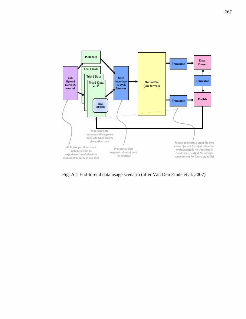
Fig. A.1 End-to-end data usage scenario (after Van Den Einde et al. 2007)
267
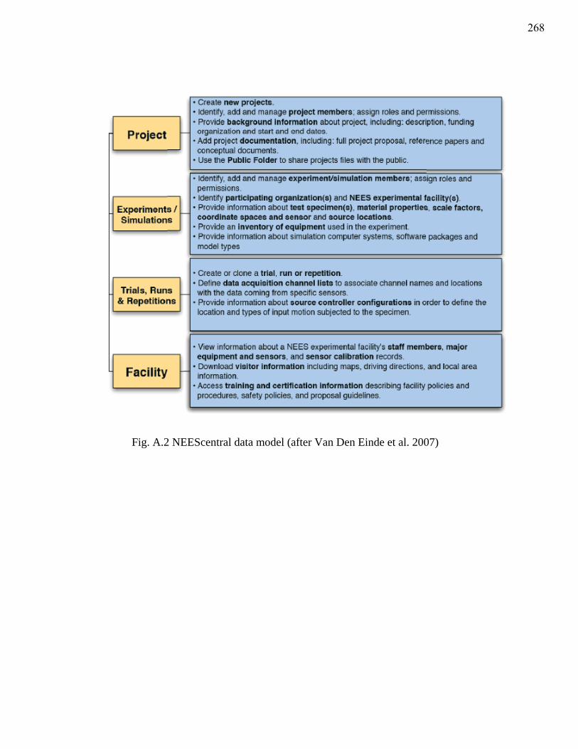
Fig. A.2 NEEScentral data model (after Van Den Einde et al. 2007)
268

Fig. A.3 Experimental data hierarchical classes in NEEScentral (after Van Den Einde et al. 2007)
269
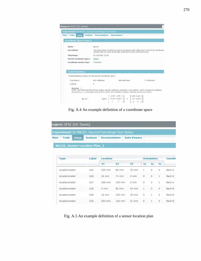
Fig. A.4 An example definition of a coordinate space
Fig. A.5 An example definition of a sensor location plan
270
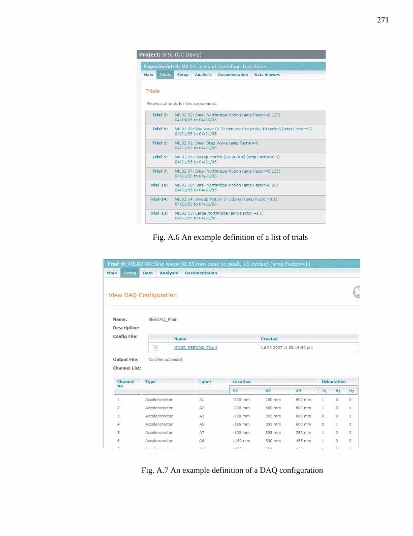
Fig. A.6 An example definition of a list of trials
Fig. A.7 An example definition of a DAQ configuration
271
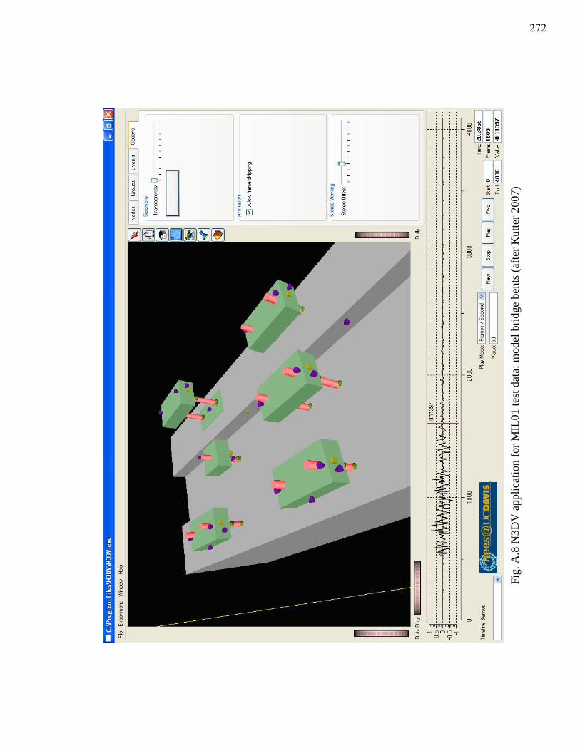
Fig.
A.8
N3D
V a
pplic
atio
n fo
r MIL
01 te
st d
ata:
mod
el b
ridge
ben
ts (a
fter K
utte
r 200
7)
272
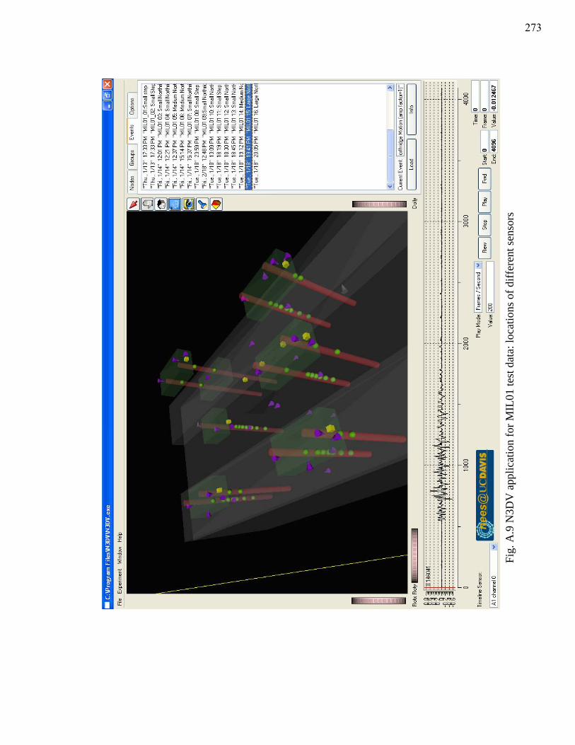
Fig.
A.9
N3D
V a
pplic
atio
n fo
r MIL
01 te
st d
ata:
loca
tions
of d
iffer
ent s
enso
rs
273
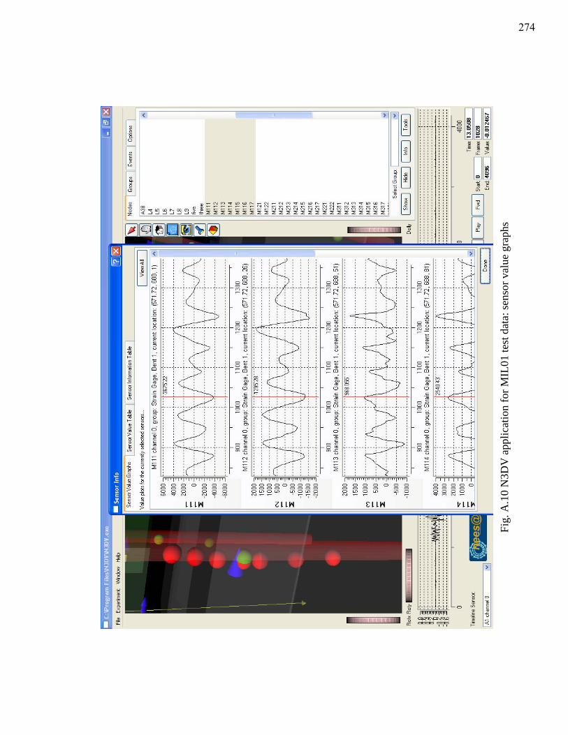
Fig.
A.1
0 N
3DV
app
licat
ion
for M
IL01
test
dat
a: se
nsor
val
ue g
raph
s
274
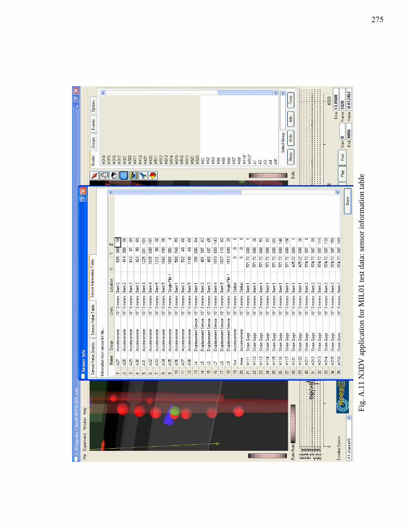
Fig.
A.1
1 N
3DV
app
licat
ion
for M
IL01
test
dat
a: se
nsor
info
rmat
ion
tabl
e
275
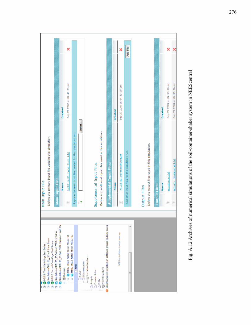
Fig.
A.1
2 A
rchi
ves o
f num
eric
al si
mul
atio
ns o
f the
soil-
cont
aine
r-sh
aker
syst
em in
NEE
Scen
tral
276