Embed Size (px)
Citation preview
Pricing Synthetic CDOs based on Exponential
Approximations to the Payoff Function∗
Ian Iscoe† Ken Jackson‡ Alex Kreinin§ Xiaofang Ma¶
April 4, 2011
Abstract
Correlation-dependent derivatives, such as Asset-Backed Securities (ABS) and Col-
lateralized Debt Obligations (CDO), are common tools for offsetting credit risk. Factor
models in the conditional independence framework are widely used in practice to capture
the correlated default events of the underlying obligors. An essential part of these models
is the accurate and efficient evaluation of the expected loss of the specified tranche, con-
ditional on a given value of a systematic factor (or values of a set of systematic factors).
Unlike other papers that focus on how to evaluate the loss distribution of the underlying
pool, in this paper we focus on the tranche loss function itself. It is approximated by a
sum of exponentials so that the conditional expectation can be evaluated in closed form
without having to evaluate the pool loss distribution. As an example, we apply this
approach to synthetic CDO pricing. Numerical results show that it is efficient.
∗This research was supported in part by the Natural Sciences and Engineering Research Council (NSERC)
of Canada.†Algorithmics Inc., 185 Spadina Avenue, Toronto, ON, M5T 2C6, Canada; [email protected]‡Department of Computer Science, University of Toronto, 10 King’s College Rd, Toronto, ON, M5S 3G4,
Canada; [email protected]§Algorithmics Inc., 185 Spadina Avenue, Toronto, ON, M5T 2C6, Canada; [email protected]¶Risk Services, CIBC, 11th Floor, 161 Bay Street, Toronto, ON, M5X 2S8, Canada; [email protected]
1
1 Introduction
Correlation-dependent derivatives, such as Asset-Backed Securities (ABS) and Collateralized
Debt Obligations (CDO), are common tools for offsetting credit risk.1 Factor models in the
conditional independence framework are widely used in practice for pricing because they are
tractable, analytic or semi-analytic formulas being available. An essential part of these models
is the accurate and efficient evaluation of the expected loss of the specified tranche, conditional
on a given value of a systematic factor (or correspondingly values of a set of systematic factors).
To be specific, the problem is how to evaluate the conditional expectation of the piecewise
linear payoff function of the loss Z
f(Z) = min(
u − ℓ, (Z − ℓ)+)
, (1)
where x+ = max(x, 0), Z =∑K
k=1 Zk, Zk are conditionally mutually independent, but not nec-
essarily identically distributed, nonnegative random variables in a conditional independence
framework (see Section 2 for explanations), and ℓ and u are the attachment and the detach-
ment points of the tranche, respectively, satisfying u > ℓ ≥ 0. Generally Zk, for obligor k, is
the product of the two components: a random variable directly related to its credit rating and
a loss-given-default or mark-to-market related value. The payoff function, f , is also known as
the stop-loss function in actuarial science [4], [23].
Note that the expectation of a function of a random variable depends on two things: the
distribution of the underlying random variable and the function itself. A standard approach
to compute the expectation of a function of a random variable is to compute firstly the
distribution of the underlying random variable, Z in our case, and then to compute the
expectation of the given function, possibly using its special properties. Almost all research in
finance [2], [9], [10], [14], [22], [25] and in actuarial science [7], [28], to name a few, has focused
on the first part due to the piecewise linearity of the payoff function.
In this paper, we propose a new approach to solving the problem. We approximate the
1For background on, and a description of, these instruments, see for example [5]. We restrict attention to
synthetic CDOs in this paper.
2
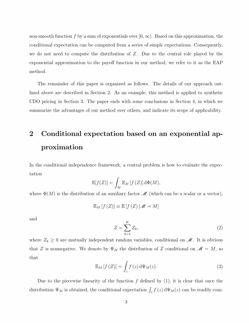
non-smooth function f by a sum of exponentials over [0,∞). Based on this approximation, the
conditional expectation can be computed from a series of simple expectations. Consequently,
we do not need to compute the distribution of Z. Due to the central role played by the
exponential approximation to the payoff function in our method, we refer to it as the EAP
method.
The remainder of this paper is organized as follows. The details of our approach out-
lined above are described in Section 2. As an example, this method is applied to synthetic
CDO pricing in Section 3. The paper ends with some conclusions in Section 4, in which we
summarize the advantages of our method over others, and indicate its scope of applicability.
2 Conditional expectation based on an exponential ap-
proximation
In the conditional independence framework, a central problem is how to evaluate the expec-
tation
E[f(Z)] =
∫
M
EM [f (Z)] dΦ(M),
where Φ(M) is the distribution of an auxiliary factor M (which can be a scalar or a vector),
EM [f (Z)] ≡ E [f (Z) |M = M ]
and
Z =K∑
k=1
Zk, (2)
where Zk ≥ 0 are mutually independent random variables, conditional on M . It is obvious
that Z is nonnegative. We denote by ΨM the distribution of Z conditional on M = M , so
that
EM [f (Z)] =
∫
z
f (z) dΨM(z). (3)
Due to the piecewise linearity of the function f defined by (1), it is clear that once the
distribution ΨM is obtained, the conditional expectation∫
zf (z) dΨM(z) can be readily com-
3

puted. Most research has focused on how to evaluate the conditional distribution of Z given
the conditional distributions of Zk. A fundamental result about a sum of independent random
variables states that Z’s conditional distribution can be computed as the convolution of Zk’s
conditional distributions. Numerically, this idea is realized through forward and inverse fast
Fourier transformations (FFT). A disadvantage of this approach is that it may be very slow
when there are many obligors due to the number of convolutions to be calculated. For pools
with special structures, it might be much slower than methods that are specially designed
for those pools, such as recursive methods proposed by De Pril [7] and Panjer [28] and their
extensions discussed in [4] and [23], and the one proposed by Jackson, Kreinin, and Ma [22]
for portfolios where the Zk sit on a properly chosen common lattice. To avoid computing too
many convolutions, the target conditional distribution can be approximated by parametric
distributions matching the first few conditional moments of the true conditional loss distri-
bution. For a large pool, a normal approximation is a natural choice as a consequence of the
central limit theorem and due to its simplicity, although it may not capture some important
properties, such as skewness and fat tails.
To capture these important properties for medium to large portfolios, compound approx-
imations, such as the compound Poisson [20], improved compound Poisson [13], compound
binomial and compound Bernoulli [29] distributions have been used. They have proved to be
very successful, since they match not only the first few conditional moments, but, most im-
portantly, they match the tails much better than either normal or normal power distributions
do. A key step in a method based on these compound approximations is the computation of
convolutions of the conditionally independent distributions of the Zk, by FFTs. As a result,
the computational complexity of such an algorithm is superlinear in K, the number of terms
in the sum (2).
As an alternative, in this paper, we propose an algorithm for which the computational
complexity is linear in K. We focus on the stop-loss function f , instead of the conditional
distribution ΨM of Z. To emphasis the role of the attachment and the detachment points ℓ
and u, we denote f(x) by f(x; ℓ, u) and introduce an auxiliary function h(x) defined on [0,∞):
4
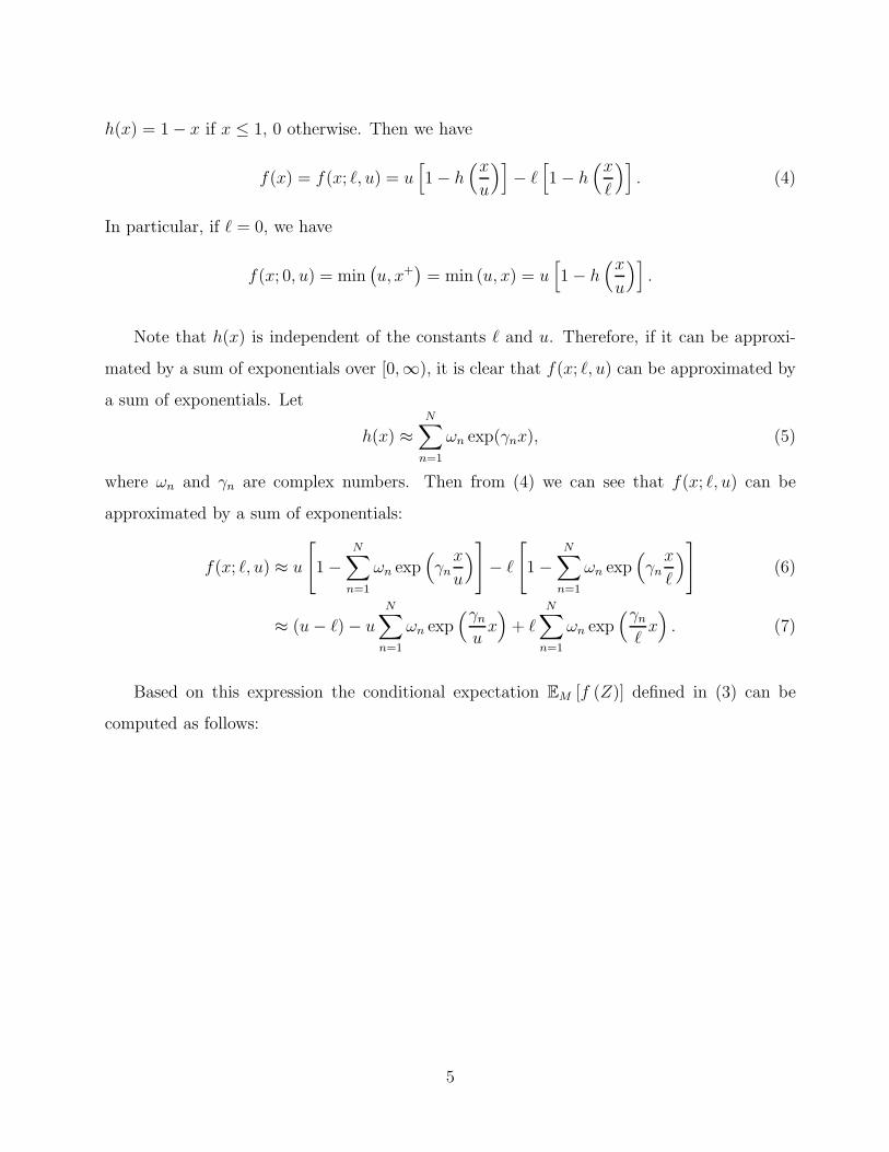
h(x) = 1 − x if x ≤ 1, 0 otherwise. Then we have
f(x) = f(x; ℓ, u) = u[
1 − h(x
u
)]
− ℓ[
1 − h(x
ℓ
)]
. (4)
In particular, if ℓ = 0, we have
f(x; 0, u) = min(
u, x+)
= min (u, x) = u[
1 − h(x
u
)]
.
Note that h(x) is independent of the constants ℓ and u. Therefore, if it can be approxi-
mated by a sum of exponentials over [0,∞), it is clear that f(x; ℓ, u) can be approximated by
a sum of exponentials. Let
h(x) ≈
N∑
n=1
ωn exp(γnx), (5)
where ωn and γn are complex numbers. Then from (4) we can see that f(x; ℓ, u) can be
approximated by a sum of exponentials:
f(x; ℓ, u) ≈ u
[
1 −N∑
n=1
ωn exp(
γn
x
u
)
]
− ℓ
[
1 −N∑
n=1
ωn exp(
γn
x
ℓ
)
]
(6)
≈ (u − ℓ) − u
N∑
n=1
ωn exp(γn
ux)
+ ℓ
N∑
n=1
ωn exp(γn
ℓx)
. (7)
Based on this expression the conditional expectation EM [f (Z)] defined in (3) can be
computed as follows:
5
EM [f (Z)]
=
∫
z
f (z) dΨM(z)
≈
∫
z
[
(u − ℓ) − u
N∑
n=1
ωn exp(γn
uz)
+ ℓ
N∑
n=1
ωn exp(γn
ℓz)
]
dΨM(z)
= (u − ℓ) − uN∑
n=1
ωn
∫
z
exp(γn
uz)
dΨM(z)
+ℓ
N∑
n=1
ωn
∫
z
exp(γn
ℓz)
dΨM(z)
= (u − ℓ)
−uN∑
n=1
ωn
∫
z1,...,zK
K∏
k=1
exp(γn
uzk
)
dΨM,1(z1) · · ·dΨM,K(zK)
+ℓ
N∑
n=1
ωn
∫
z1,...,zK
K∏
k=1
exp(γn
ℓzk
)
dΨM,1(z1) · · ·dΨM,K(zK)
= (u − ℓ) − uN∑
n=1
ωn
K∏
k=1
EM
[
exp(γn
uZk
)]
+ℓ
N∑
n=1
ωn
K∏
k=1
EM
[
exp(γn
ℓZk
)]
, (8)
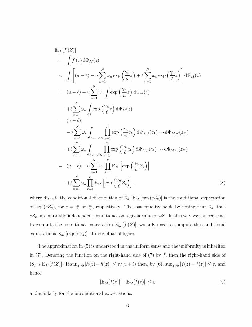
where ΨM,k is the conditional distribution of Zk, EM [exp (cZk)] is the conditional expectation
of exp (cZk), for c = γn
ℓor γn
u, respectively. The last equality holds by noting that Zk, thus
cZk, are mutually independent conditional on a given value of M . In this way we can see that,
to compute the conditional expectation EM [f (Z)], we only need to compute the conditional
expectations EM [exp (cZk)] of individual obligors.
The approximation in (5) is understood in the uniform sense and the uniformity is inherited
in (7). Denoting the function on the right-hand side of (7) by f , then the right-hand side of
(8) is EM [f(Z)]. If supz≥0 |h(z)− h(z)| ≤ ε/(u + ℓ) then, by (6), supz≥0 |f(z)− f(z)| ≤ ε, and
hence
|EM [f(z)] − EM [f(z)]| ≤ ε (9)
and similarly for the unconditional expectations.
6
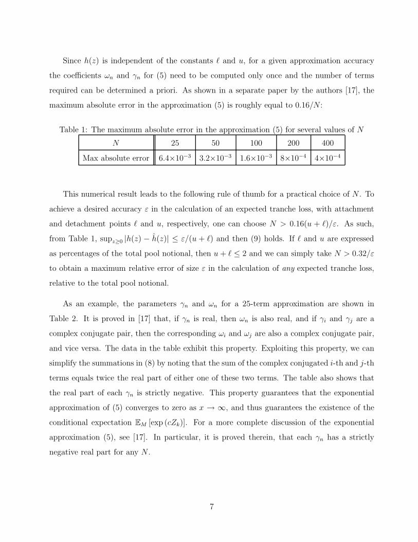
Since h(z) is independent of the constants ℓ and u, for a given approximation accuracy
the coefficients ωn and γn for (5) need to be computed only once and the number of terms
required can be determined a priori. As shown in a separate paper by the authors [17], the
maximum absolute error in the approximation (5) is roughly equal to 0.16/N :
Table 1: The maximum absolute error in the approximation (5) for several values of N
N 25 50 100 200 400
Max absolute error 6.4×10⁻³ 3.2×10⁻³ 1.6×10⁻³ 8×10⁻⁴ 4×10⁻⁴
This numerical result leads to the following rule of thumb for a practical choice of N . To
achieve a desired accuracy ε in the calculation of an expected tranche loss, with attachment
and detachment points ℓ and u, respectively, one can choose N > 0.16(u + ℓ)/ε. As such,
from Table 1, supz≥0 |h(z) − h(z)| ≤ ε/(u + ℓ) and then (9) holds. If ℓ and u are expressed
as percentages of the total pool notional, then u + ℓ ≤ 2 and we can simply take N > 0.32/ε
to obtain a maximum relative error of size ε in the calculation of any expected tranche loss,
relative to the total pool notional.
As an example, the parameters γn and ωn for a 25-term approximation are shown in
Table 2. It is proved in [17] that, if γn is real, then ωn is also real, and if γi and γj are a
complex conjugate pair, then the corresponding ωi and ωj are also a complex conjugate pair,
and vice versa. The data in the table exhibit this property. Exploiting this property, we can
simplify the summations in (8) by noting that the sum of the complex conjugated i-th and j-th
terms equals twice the real part of either one of these two terms. The table also shows that
the real part of each γn is strictly negative. This property guarantees that the exponential
approximation of (5) converges to zero as x → ∞, and thus guarantees the existence of the
conditional expectation EM [exp (cZk)]. For a more complete discussion of the exponential
approximation (5), see [17]. In particular, it is proved therein, that each γn has a strictly
negative real part for any N .
7

Table 2: The real and imaginary parts of ωn and γn (weights and exponents) for the 25-term
exponential approximation
n ℜ(ωn) ℑ(ωn) ℜ(γn) ℑ(γn)
1 1.68E-4 -3.16E-5 -5.68E-2 1.45E+2
2 1.68E-4 3.16E-5 -5.68E-2 -1.45E+2
3 2.04E-4 -5.98E-5 -1.72E-1 1.32E+2
4 2.04E-4 5.98E-5 -1.72E-1 -1.32E+2
5 2.69E-4 -1.02E-4 -3.51E-1 1.20E+2
6 2.69E-4 1.02E-4 -3.51E-1 -1.20E+2
7 3.87E-4 -1.70E-4 -5.98E-1 1.07E+2
8 3.87E-4 1.70E-4 -5.98E-1 -1.07E+2
9 6.02E-4 -2.94E-4 -9.25E-1 9.49E+1
10 6.02E-4 2.94E-4 -9.25E-1 -9.49E+1
11 1.01E-3 -5.39E-4 -1.35E+0 8.24E+1
12 1.01E-3 5.39E-4 -1.35E+0 -8.24E+1
13 1.87E-3 -1.09E-3 -1.89E+0 6.99E+1
14 1.87E-3 1.09E-3 -1.89E+0 -6.99E+1
15 3.86E-3 -2.53E-3 -2.58E+0 5.74E+1
16 3.86E-3 2.53E-3 -2.58E+0 -5.74E+1
17 9.17E-3 -7.44E-3 -3.50E+0 4.49E+1
18 9.17E-3 7.44E-3 -3.50E+0 -4.49E+1
19 2.45E-2 -3.19E-2 -4.73E+0 3.24E+1
20 2.45E-2 3.19E-2 -4.73E+0 -3.24E+1
21 7.57E-3 -2.10E-1 -6.44E+0 2.04E+1
22 7.57E-3 2.10E-1 -6.44E+0 -2.04E+1
23 3.81E+0 0.00E+0 -9.65E+0 0.00E+0
24 -1.46E+0 1.03E-1 -8.54E+0 9.38E+0
25 -1.46E+0 -1.03E-1 -8.54E+0 -9.38E+0
8

3 Pricing synthetic CDOs
We illustrate the EAP method by applying it to synthetic CDO pricing. The underlying
collateral of a synthetic CDO is a set of credit default swaps (CDSs).
3.1 Overview of models and pricing methods
Factor models, such as the reduced-form model proposed by Laurent and Gregory [25] or the
one proposed by Duffie and Garleanu [10] and extended successively by Mortensen [27] and
Eckner [11], and the structural model proposed by Vasicek [31] and Li [26], are widely used
in practice to obtain analytic or semi-analytic formulas to price synthetic CDOs efficiently.
For a comparative analysis of different copula models, see the paper by Burtschell, Gregory
and Laurent [6]. A generalization of the reduced-form model which, along with the structural
model, can capture credit-state migration, is the affine Markov model proposed by Hurd and
Kuznetsov [16] and used by them in pricing CDOs in [15].
Some exact and approximate methods for loss-distribution evaluation have been studied in
[22]. There are also Fourier transform related methods. In particular, the saddle point approx-
imation method2 was applied by Antonov, Mechkov, and Misirpashaev [3] and Yang, Hurd
and Zhang [32], for pricing CDOs. Here we apply the exponential-approximation method, as
described in the previous section, to synthetic CDO pricing.
3.2 The pricing equation and the Gaussian copula model
To illustrate our method, we use a simple one-factor Gaussian copula model. Examples of
other models, to which the EAP method is applicable, are given in the Conclusion, Section 4.
It is assumed that the interest rates are deterministic and the recovery rate corresponding to
2In principle, this method is applicable to large pools, as the pool size plays the role of the large parameter
(albeit not in the classical multiplicative manner) in the inverse Fourier integrand’s exponent to which the
saddle point method is applied.
9
each underlying name is constant. Let 0 < t1 < t2 < · · · < tn = T be the set of premium
dates, with T denoting the maturity of the CDO, and d1, d2, . . . , dn be the set of corresponding
discount factors. Suppose there are K names in the pool with recovery-adjusted notional
values LGD1, LGD2, . . . , LGDK in properly chosen units. Let L Pi be the pool’s cumulative
losses up to time ti and ℓ be the attachment point of a specified tranche of thickness S. An
attachment point of a tranche is a threshold that determines whether some losses of the pool
shall be absorbed by this tranche, i.e., if the realized losses of the pool are less than ℓ, then
the tranche will not suffer any loss, otherwise it will absorb an amount up to S. Accordingly,
the detachment point of the tranche is u = S + ℓ. Thus the loss absorbed by the specified
tranche up to time ti is Li = min(
S, (L Pi − ℓ)+
)
. If we further assume the fair spread s for
the tranche is a constant, then it can be calculated from the equation (see e.g., [8], [20])
s =E [∑n
i=1(Li − Li−1)di]
E [∑n
i=1(S − Li)(ti − ti−1)di]=
∑n
i=1 E [(Li − Li−1)di]∑n
i=1 E [(S − Li)(ti − ti−1)di], (10)
with t0 = 0 and E [L0] = 0.
Assuming the discount factors di are independent of the L Pj , it follows from (10) that the
problem of computing the fair spread s reduces to evaluating the expected cumulative losses
E [Li], i = 1, 2, . . . , n. In order to compute this expectation, we have to specify the default
processes for each name and the correlation structure of the default events. One-factor models
were first introduced by Vasicek [31] to estimate the loan loss distribution and then generalized
by Li [26], Gordy and Jones [12], Hull and White [14], Iscoe, Kreinin and Rosen [21], Laurent
and Gregory [25], and Schonbucher [30], to name a few.
Let τk be the default time of name k. Assume the risk-neutral default probabilities πk(t) =
P (τk < t), k = 1, 2, . . . , K, that describe the default-time distributions of all K names are
available, where τk and t take discrete values from {t1, t2, . . . , tn}. The dependence structure
of the default times are determined in terms of their creditworthiness indices Yk, which are
defined by
Yk = βkX + σkεk, k = 1, 2, . . . , K, (11)
where X is the systematic risk factor, εk are idiosyncratic factors that are mutually indepen-
dent and are also independent of X; βk and σk are constants satisfying the relation β2k +σ2
k = 1.
10
These risk-neutral default probabilities and the creditworthiness indices are related by the
threshold model
πk(t) = P (τk < t) = P (Yk < Hk(t)) , (12)
where Hk(t) is the default barrier of the k-th name at time t.
Thus the correlation structure of default events is captured by the systematic risk factor X.
Conditional on a given value x of X, all default events are independent. If we further assume,
as we do, that X and εk follow the standard normal distribution, then Yk is a standard normal
random variable and from (12) we have Hk(t) = Φ−1 (πk(t)). Furthermore, the correlation
between two different indices Yi and Yj is βiβj .
The conditional, risk-neutral default-time distribution is defined by
πk(t; x) = P (Yk < Hk(t)|X = x) . (13)
Thus from (11) and (13) we have
πk(t; x) = Φ
(
Hk(t) − βkx
σk
)
. (14)
The conditional and unconditional risk-neutral default-time probabilities at the premium date
ti are denoted by πk(i; x) and πk(i), respectively.
In this conditional independence framework, the expected cumulative tranche losses E [Li]
can be computed as
E [Li] =
∫ ∞
−∞
Ex [Li] dΦ(x), (15)
where Ex [Li] = Ex
[
min(
S, (L Pi − ℓ)+
)]
is the expectation of Li conditional on the value of
X being x, where L Pi =
∑K
k=1 LGDk1{Yk<Hk(ti)}, and the indicators 1{Yk<Hk(ti)} are mutu-
ally independent conditional on X. Generally, the integration in (15) needs to be evaluated
numerically using an appropriate quadrature rule:
E [Li] ≈M∑
m=1
wmExm
[
min(
S, (L Pi − ℓ)+
)]
. (16)
In the notation of Section 2, Z = L Pi , Zk = LGDk1{Yk<Hk(ti)}, and M = X.
11
3.3 CDO pricing based on the exponential approximation
Notice from formula (16) that the fundamental problem in CDO pricing is how to evaluate
the conditional expected loss Exm
[
min(
S, (L Pi − ℓ)+
)]
with a given value xm of X. Since
min(
S, (L Pi − ℓ)+
)
= f(L Pi ; ℓ, ℓ + S), (17)
from (7) we see that
min(
S, (L Pi − ℓ)+
)
≈(ℓ + S)
[
1 −N∑
n=1
ωn exp
(
γn
L Pi
ℓ + S
)
]
− ℓ
[
1 −N∑
n=1
ωn exp
(
γn
L Pi
ℓ
)
]
=S − (ℓ + S)
N∑
n=1
ωn exp
(
γn
ℓ + SL
Pi
)
+ ℓ
N∑
n=1
ωn exp(γn
ℓL
Pi
)
.
As a special case of (8) we have
Exm
[
min(
S, (L Pi − ℓ)+
)]
≈S − (ℓ + S)
N∑
n=1
ωnExm
[
exp
(
γn
ℓ + S
K∑
k=1
LGDk1{Yk<Hk(ti)}
)]
+ ℓN∑
n=1
ωnExm
[
exp
(
γn
ℓ
K∑
k=1
LGDk1{Yk<Hk(ti)}
)]
=S − (ℓ + S)
N∑
n=1
ωn
K∏
k=1
Exm
[
exp
(
γn
ℓ + SLGDk1{Yk<Hk(ti)}
)]
+ ℓN∑
n=1
ωn
K∏
k=1
Exm
[
exp(γn
ℓLGDk1{Yk<Hk(ti)}
)]
, (18)
where
Exm
[
exp
(
γn
ℓ + SLGDk1{Yk<Hk(ti)}
)]
= πk(i; xm) exp
(
γn
ℓ + SLGDk
)
+ (1 − πk(i; xm)) ,
Exm
[
exp(γn
ℓLGDk1{Yk<Hk(ti)}
)]
= πk(i; xm) exp(γn
ℓLGDk
)
+ (1 − πk(i; xm)) ,
since 1{Yk<Hk(ti)} = 1 with probability πk(i; xm) and 0 with probability 1 − πk(i; xm), and
LGDk is a constant.
3.4 Numerical results
In this section we present numerical results comparing the accuracy and the computational
time for EAP and the exact method, which we denote by JKM, proposed in [22]. The results
12
presented below are based on a sample of 15 = 3×5 pools: three pool sizes (100, 200, 400) and,
for each size, five different types in terms of the notional values of the underlying reference
entities. The possible notional values for each pool are summarized in Table 3. The number
of reference entities is the same in each of the homogeneous subgroups in a given pool. For
example, for a 200-name pool of type 3, there are four homogeneous subgroups each with
50 reference entities of notional values 50, 100, 150, and 200, respectively. Thus, the higher
the pool type, the more heterogeneous is the pool, with pool type 1 indicating a completely
homogeneous pool in terms of notional values. In the figures and tables that follow, the label
K-m denotes a pool of size K and pool type m.
Table 3: Selection of notional values of K-name pools
Pool Type 1 2 3 4 5
Notional values 100 50, 100 50, 100, 150, 200 20, 50, 100, 150, 200 10, 20, . . . , K
For each name, the common risk-neutral cumulative default probabilities are given in
Table 4.
Table 4: Risk-neutral cumulative default probabilities
Time 1 yr. 2 yrs. 3 yrs. 4 yrs. 5 yrs.
Prob. 0.0072 0.0185 0.0328 0.0495 0.0680
The recovery rate is assumed to be 40% for all names. Thus the LGD of name k is
0.6Nk. The maturity of a CDO deal is five years (i.e., T = 5) and the premium dates are
ti = i, i = 1, . . . , 5 years from today (t0 = 0). The continuously compounded interest rates
are r1 = 4.6%, r2 = 5%, r3 = 5.6%, r4 = 5.8% and r5 = 6%. Thus the corresponding discount
factors, defined by di = exp(−tiri), are 0.9550, 0.9048, 0.8454, 0.7929 and 0.7408, respectively.
All CDO pools have five tranches that are determined by the attachment points (ℓ’s) of the
tranches. For this experiment, the five attachment points are: 0, 3%, 7%, 10% and 15%, with
the last detachment point being 30%. The constants βk are all 0.5. (In practice, the βk’s are
13
known as sensitivities and are calibrated to market data. Here they are simply taken as input
to the model, for the purpose of numerical experimentation.)
All methods for this experiment were coded in Matlab and the programs were run on a
Pentium D 925 PC. The results are presented in Tables 5, 6 and 7.
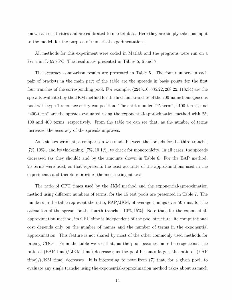
The accuracy comparison results are presented in Table 5. The four numbers in each
pair of brackets in the main part of the table are the spreads in basis points for the first
four tranches of the corresponding pool. For example, (2248.16, 635.22, 268.22, 118.34) are the
spreads evaluated by the JKM method for the first four tranches of the 200-name homogeneous
pool with type 1 reference entity composition. The entries under “25-term”, “100-term”, and
“400-term” are the spreads evaluated using the exponential-approximation method with 25,
100 and 400 terms, respectively. From the table we can see that, as the number of terms
increases, the accuracy of the spreads improves.
As a side-experiment, a comparison was made between the spreads for the third tranche,
[7%, 10%], and its thickening, [7%, 10.1%], to check for monotonicity. In all cases, the spreads
decreased (as they should) and by the amounts shown in Table 6. For the EAP method,
25 terms were used, as that represents the least accurate of the approximations used in the
experiments and therefore provides the most stringent test.
The ratio of CPU times used by the JKM method and the exponential-approximation
method using different numbers of terms, for the 15 test pools are presented in Table 7. The
numbers in the table represent the ratio, EAP/JKM, of average timings over 50 runs, for the
calcuation of the spread for the fourth tranche, [10%, 15%]. Note that, for the exponential-
approximation method, its CPU time is independent of the pool structure: its computational
cost depends only on the number of names and the number of terms in the exponential
approximation. This feature is not shared by most of the other commonly used methods for
pricing CDOs. From the table we see that, as the pool becomes more heterogeneous, the
ratio of (EAP time)/(JKM time) decreases; as the pool becomes larger, the ratio of (EAP
time)/(JKM time) decreases. It is interesting to note from (7) that, for a given pool, to
evaluate any single tranche using the exponential-approximation method takes about as much
14
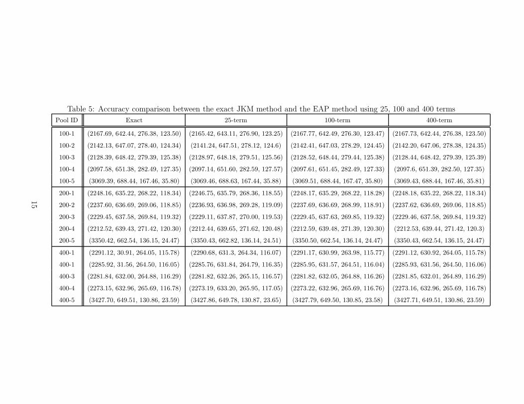
Table 5: Accuracy comparison between the exact JKM method and the EAP method using 25, 100 and 400 terms
Pool ID Exact 25-term 100-term 400-term
100-1 (2167.69, 642.44, 276.38, 123.50) (2165.42, 643.11, 276.90, 123.25) (2167.77, 642.49, 276.30, 123.47) (2167.73, 642.44, 276.38, 123.50)
100-2 (2142.13, 647.07, 278.40, 124.34) (2141.24, 647.51, 278.12, 124.6) (2142.41, 647.03, 278.29, 124.45) (2142.20, 647.06, 278.38, 124.35)
100-3 (2128.39, 648.42, 279.39, 125.38) (2128.97, 648.18, 279.51, 125.56) (2128.52, 648.44, 279.44, 125.38) (2128.44, 648.42, 279.39, 125.39)
100-4 (2097.58, 651.38, 282.49, 127.35) (2097.14, 651.60, 282.59, 127.57) (2097.61, 651.45, 282.49, 127.33) (2097.6, 651.39, 282.50, 127.35)
100-5 (3069.39, 688.44, 167.46, 35.80) (3069.46, 688.63, 167.44, 35.88) (3069.51, 688.44, 167.47, 35.80) (3069.43, 688.44, 167.46, 35.81)
200-1 (2248.16, 635.22, 268.22, 118.34) (2246.75, 635.79, 268.36, 118.55) (2248.17, 635.29, 268.22, 118.28) (2248.18, 635.22, 268.22, 118.34)
200-2 (2237.60, 636.69, 269.06, 118.85) (2236.93, 636.98, 269.28, 119.09) (2237.69, 636.69, 268.99, 118.91) (2237.62, 636.69, 269.06, 118.85)
200-3 (2229.45, 637.58, 269.84, 119.32) (2229.11, 637.87, 270.00, 119.53) (2229.45, 637.63, 269.85, 119.32) (2229.46, 637.58, 269.84, 119.32)
200-4 (2212.52, 639.43, 271.42, 120.30) (2212.44, 639.65, 271.62, 120.48) (2212.59, 639.48, 271.39, 120.30) (2212.53, 639.44, 271.42, 120.3)
200-5 (3350.42, 662.54, 136.15, 24.47) (3350.43, 662.82, 136.14, 24.51) (3350.50, 662.54, 136.14, 24.47) (3350.43, 662.54, 136.15, 24.47)
400-1 (2291.12, 30.91, 264.05, 115.78) (2290.68, 631.3, 264.34, 116.07) (2291.17, 630.99, 263.98, 115.77) (2291.12, 630.92, 264.05, 115.78)
400-1 (2285.92, 31.56, 264.50, 116.05) (2285.76, 631.84, 264.79, 116.35) (2285.95, 631.57, 264.51, 116.04) (2285.93, 631.56, 264.50, 116.06)
400-3 (2281.84, 632.00, 264.88, 116.29) (2281.82, 632.26, 265.15, 116.57) (2281.82, 632.05, 264.88, 116.26) (2281.85, 632.01, 264.89, 116.29)
400-4 (2273.15, 632.96, 265.69, 116.78) (2273.19, 633.20, 265.95, 117.05) (2273.22, 632.96, 265.69, 116.76) (2273.16, 632.96, 265.69, 116.78)
400-5 (3427.70, 649.51, 130.86, 23.59) (3427.86, 649.78, 130.87, 23.65) (3427.79, 649.50, 130.85, 23.58) (3427.71, 649.51, 130.86, 23.59)
15
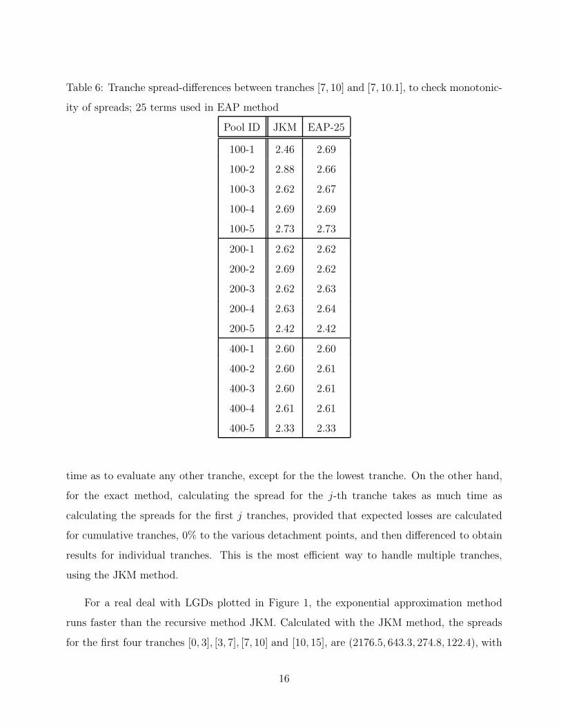
Table 6: Tranche spread-differences between tranches [7, 10] and [7, 10.1], to check monotonic-
ity of spreads; 25 terms used in EAP method
Pool ID JKM EAP-25
100-1 2.46 2.69
100-2 2.88 2.66
100-3 2.62 2.67
100-4 2.69 2.69
100-5 2.73 2.73
200-1 2.62 2.62
200-2 2.69 2.62
200-3 2.62 2.63
200-4 2.63 2.64
200-5 2.42 2.42
400-1 2.60 2.60
400-2 2.60 2.61
400-3 2.60 2.61
400-4 2.61 2.61
400-5 2.33 2.33
time as to evaluate any other tranche, except for the the lowest tranche. On the other hand,
for the exact method, calculating the spread for the j-th tranche takes as much time as
calculating the spreads for the first j tranches, provided that expected losses are calculated
for cumulative tranches, 0% to the various detachment points, and then differenced to obtain
results for individual tranches. This is the most efficient way to handle multiple tranches,
using the JKM method.
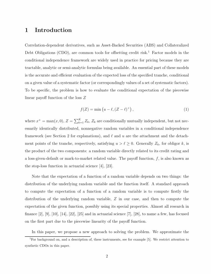
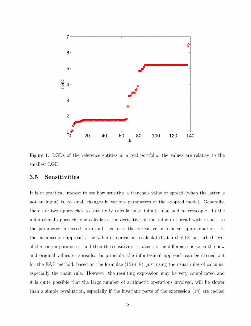
For a real deal with LGDs plotted in Figure 1, the exponential approximation method
runs faster than the recursive method JKM. Calculated with the JKM method, the spreads
for the first four tranches [0, 3], [3, 7], [7, 10] and [10, 15], are (2176.5, 643.3, 274.8, 122.4), with
16
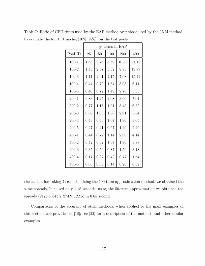
Table 7: Ratio of CPU times used by the EAP method over those used by the JKM method,
to evaluate the fourth tranche, [10%, 15%], on the test pools
# terms in EAP
Pool ID 25 50 100 200 400
100-1 1.65 2.75 5.69 10.53 21.12
100-2 1.43 2.57 5.32 9.85 19.77
100-3 1.11 2.01 4.15 7.68 15.42
100-4 0.44 0.79 1.64 3.05 6.11
100-5 0.40 0.72 1.49 2.76 5.53
200-1 0.83 1.25 2.08 3.66 7.01
200-2 0.77 1.18 1.91 3.43 6.52
200-3 0.66 1.03 1.68 2.91 5.64
200-4 0.43 0.66 1.07 1.90 3.65
200-5 0.27 0.41 0.67 1.20 2.29
400-1 0.44 0.72 1.14 2.08 4.14
400-2 0.42 0.62 1.07 1.96 3.87
400-3 0.35 0.56 0.87 1.59 3.18
400-4 0.17 0.27 0.42 0.77 1.54
400-5 0.06 0.08 0.14 0.26 0.52
the calculation taking 7 seconds. Using the 100-term approximation method, we obtained the
same spreads, but used only 1.18 seconds; using the 50-term approximation we obtained the
spreads (2176.5, 643.2, 274.9, 122.5) in 0.65 second.
Comparisons of the accuracy of other methods, when applied to the main examples of
this section, are provided in [18]; see [22] for a description of the methods and other similar
examples.
17
0 20 40 60 80 100 120 1401
2
3
4
5
6
7
k
LGD
Figure 1: LGDs of the reference entities in a real portfolio, the values are relative to the
smallest LGD
3.5 Sensitivities
It is of practical interest to see how sensitive a tranche’s value or spread (when the latter is
not an input) is, to small changes in various parameters of the adopted model. Generally,
there are two approaches to sensitivity calculations: infinitesimal and macroscopic. In the
infinitesimal approach, one calculates the derivative of the value or spread with respect to
the parameter in closed form and then uses the derivative in a linear approximation. In
the macroscopic approach, the value or spread is recalculated at a slightly perturbed level
of the chosen parameter, and then the sensitivity is taken as the difference between the new
and original values or spreads. In principle, the infinitesimal approach can be carried out
for the EAP method, based on the formulae (15)-(18), just using the usual rules of calculus,
especially the chain rule. However, the resulting expression may be very complicated and
it is quite possible that the large number of arithmetic operations involved, will be slower
than a simple revaluation, especially if the invariant parts of the expression (18) are cached
18
and available during the revaluation. Of course, the identity of the parameter being tweaked,
has a strong influence on the result of the comparison of the two approaches. For example,
the formula resulting from tweaking a LGD is much less complicated than one resulting from
tweaking a PD. For the sake of generality, we will follow the macroscopic approach and restrict
attention to the accuracy of spread sensitivities calculated with the EAP method, for the sake
of concreteness, comparing the results to the benchmark JKM method.
Of all the model parameters that can be perturbed or tweaked, the probabilities of default
are the most interesting ones, especially as they affect all tranches.3 Specifically, we will
continue with the 15-pool examples of the previous section and study numerically the result
of subjecting the probablity of default (PD) curve to a positive parallel shift of 20 bp. The
results for the alternative choices of 10 bp and 5 bp, for the parallel shift, are similar and
described in detail in [19]. In Figures 2–5, the pool size 100 (respectively, 200, 400) is indicated
by a solid (respectively, dashed, dot-dashed) line while the pool type 1 (respectively, 2, 3, 4,
5) is indicated by the marker � (respectively, �, N, H, ◮).
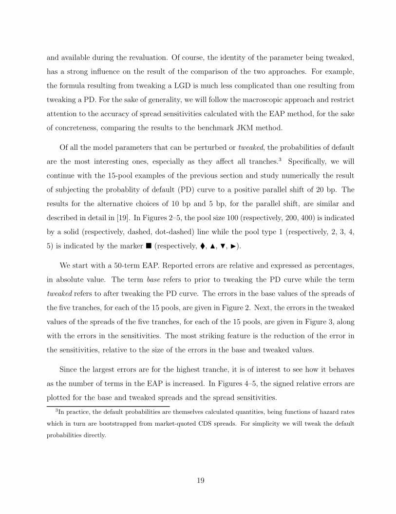
We start with a 50-term EAP. Reported errors are relative and expressed as percentages,
in absolute value. The term base refers to prior to tweaking the PD curve while the term
tweaked refers to after tweaking the PD curve. The errors in the base values of the spreads of
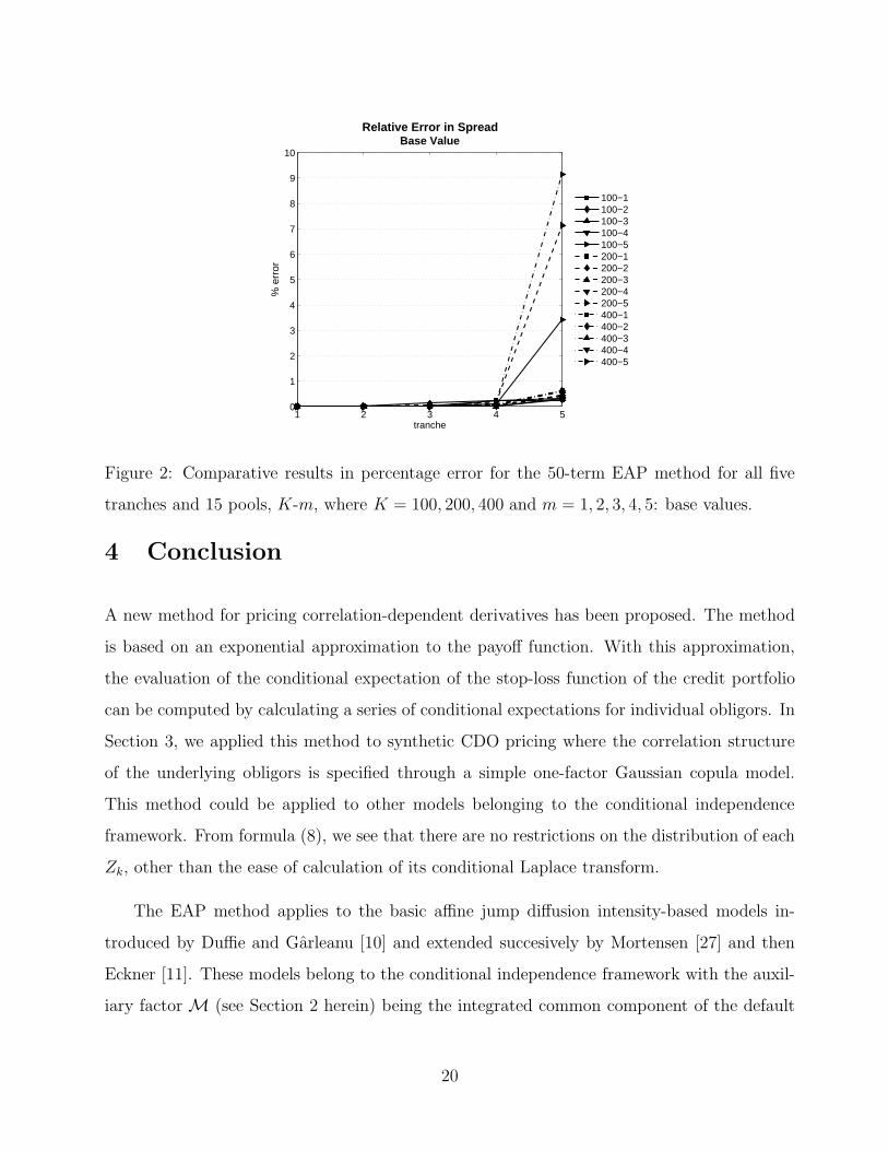
the five tranches, for each of the 15 pools, are given in Figure 2. Next, the errors in the tweaked
values of the spreads of the five tranches, for each of the 15 pools, are given in Figure 3, along
with the errors in the sensitivities. The most striking feature is the reduction of the error in
the sensitivities, relative to the size of the errors in the base and tweaked values.
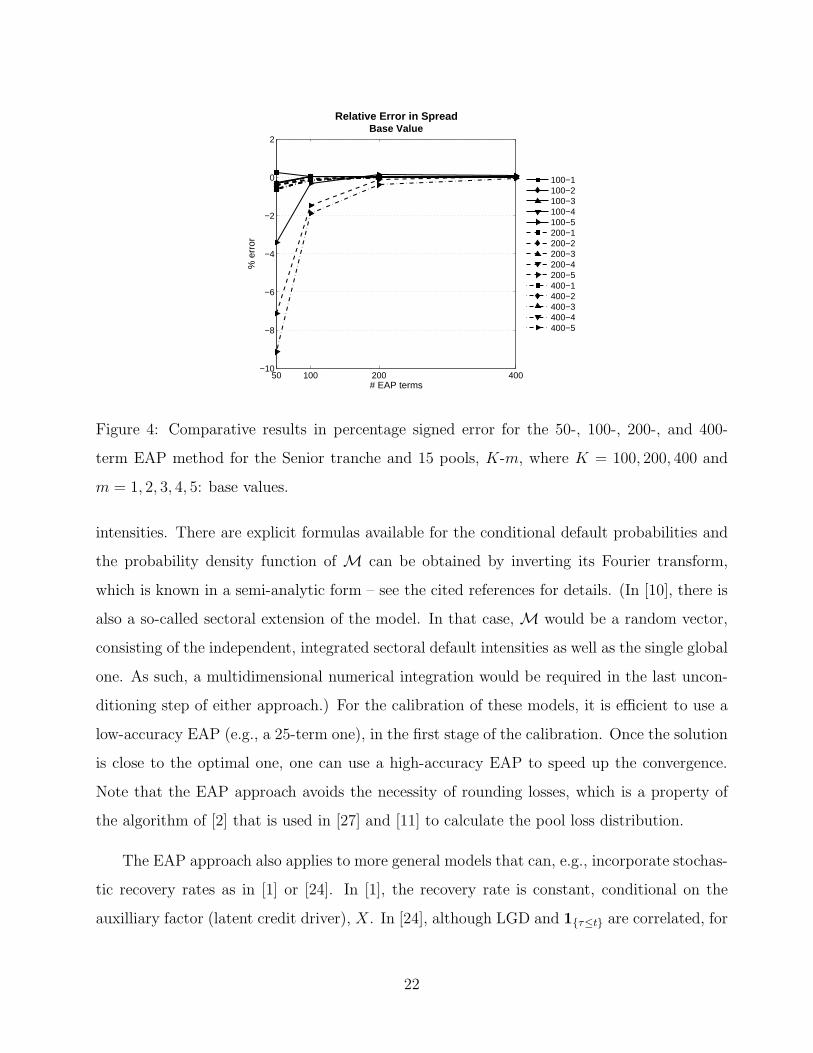
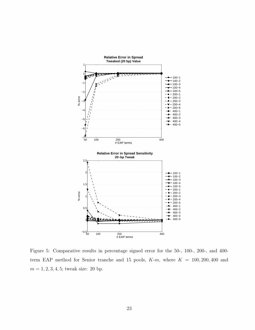
Since the largest errors are for the highest tranche, it is of interest to see how it behaves
as the number of terms in the EAP is increased. In Figures 4–5, the signed relative errors are
plotted for the base and tweaked spreads and the spread sensitivities.
3In practice, the default probabilities are themselves calculated quantities, being functions of hazard rates
which in turn are bootstrapped from market-quoted CDS spreads. For simplicity we will tweak the default
probabilities directly.
19
1 2 3 4 50
1
2
3
4
5
6
7
8
9
10
Relative Error in SpreadBase Value
tranche
% e
rror
100−1100−2100−3100−4100−5200−1200−2200−3200−4200−5400−1400−2400−3400−4400−5
Figure 2: Comparative results in percentage error for the 50-term EAP method for all five
tranches and 15 pools, K-m, where K = 100, 200, 400 and m = 1, 2, 3, 4, 5: base values.
4 Conclusion
A new method for pricing correlation-dependent derivatives has been proposed. The method
is based on an exponential approximation to the payoff function. With this approximation,
the evaluation of the conditional expectation of the stop-loss function of the credit portfolio
can be computed by calculating a series of conditional expectations for individual obligors. In
Section 3, we applied this method to synthetic CDO pricing where the correlation structure
of the underlying obligors is specified through a simple one-factor Gaussian copula model.
This method could be applied to other models belonging to the conditional independence
framework. From formula (8), we see that there are no restrictions on the distribution of each
Zk, other than the ease of calculation of its conditional Laplace transform.
The EAP method applies to the basic affine jump diffusion intensity-based models in-
troduced by Duffie and Garleanu [10] and extended succesively by Mortensen [27] and then
Eckner [11]. These models belong to the conditional independence framework with the auxil-
iary factor M (see Section 2 herein) being the integrated common component of the default
20
1 2 3 4 50
1
2
3
4
5
6
7
Relative Error in SpreadTweaked (20 bp) Value
tranche
% e
rror
100−1100−2100−3100−4100−5200−1200−2200−3200−4200−5400−1400−2400−3400−4400−5
1 2 3 4 50
0.5
1
1.5
2
2.5
Relative Error in Spread Sensitivity20−bp Tweak
tranche
% e
rror
100−1100−2100−3100−4100−5200−1200−2200−3200−4200−5400−1400−2400−3400−4400−5
Figure 3: Comparative results in percentage error for the 50-term EAP method for all five
tranches and 15 pools, K-m, where K = 100, 200, 400 and m = 1, 2, 3, 4, 5; tweak size: 20 bp.
21
50 100 200 400−10
−8
−6
−4
−2
0
2
Relative Error in SpreadBase Value
# EAP terms
% e
rror
100−1100−2100−3100−4100−5200−1200−2200−3200−4200−5400−1400−2400−3400−4400−5
Figure 4: Comparative results in percentage signed error for the 50-, 100-, 200-, and 400-
term EAP method for the Senior tranche and 15 pools, K-m, where K = 100, 200, 400 and
m = 1, 2, 3, 4, 5: base values.
intensities. There are explicit formulas available for the conditional default probabilities and
the probability density function of M can be obtained by inverting its Fourier transform,
which is known in a semi-analytic form – see the cited references for details. (In [10], there is
also a so-called sectoral extension of the model. In that case, M would be a random vector,
consisting of the independent, integrated sectoral default intensities as well as the single global
one. As such, a multidimensional numerical integration would be required in the last uncon-
ditioning step of either approach.) For the calibration of these models, it is efficient to use a
low-accuracy EAP (e.g., a 25-term one), in the first stage of the calibration. Once the solution
is close to the optimal one, one can use a high-accuracy EAP to speed up the convergence.
Note that the EAP approach avoids the necessity of rounding losses, which is a property of
the algorithm of [2] that is used in [27] and [11] to calculate the pool loss distribution.
The EAP approach also applies to more general models that can, e.g., incorporate stochas-
tic recovery rates as in [1] or [24]. In [1], the recovery rate is constant, conditional on the
auxilliary factor (latent credit driver), X. In [24], although LGD and 1{τ≤t} are correlated, for
22
50 100 200 400−7
−6
−5
−4
−3
−2
−1
0
1
Relative Error in SpreadTweaked (20 bp) Value
# EAP terms
% e
rror
100−1100−2100−3100−4100−5200−1200−2200−3200−4200−5400−1400−2400−3400−4400−5
50 100 200 400−0.5
0
0.5
1
1.5
2
2.5
Relative Error in Spread Sensitivity20−bp Tweak
# EAP terms
% e
rror
100−1100−2100−3100−4100−5200−1200−2200−3200−4200−5400−1400−2400−3400−4400−5
Figure 5: Comparative results in percentage signed error for the 50-, 100-, 200-, and 400-
term EAP method for Senior tranche and 15 pools, K-m, where K = 100, 200, 400 and
m = 1, 2, 3, 4, 5; tweak size: 20 bp.
23
each obligor, the LGD and the indicator function depend on the same Y , the creditworthiness
of the obligor; and the definition of LGD is explicit. Thus we can compute the conditional
expectation, E[LGD1{τ≤t} |X], explicitly.
Here is a summary of the advantages and disadvantages of the EAP method, as applied
to synthetic CDOs.
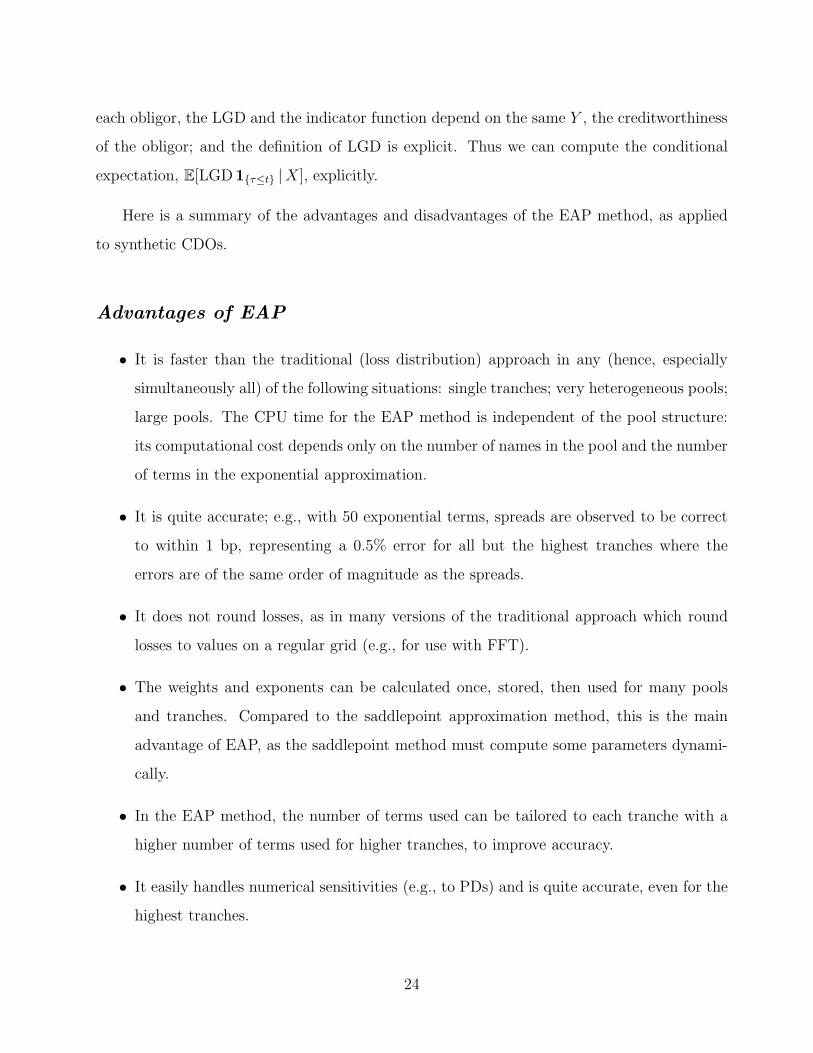
Advantages of EAP
• It is faster than the traditional (loss distribution) approach in any (hence, especially
simultaneously all) of the following situations: single tranches; very heterogeneous pools;
large pools. The CPU time for the EAP method is independent of the pool structure:
its computational cost depends only on the number of names in the pool and the number
of terms in the exponential approximation.
• It is quite accurate; e.g., with 50 exponential terms, spreads are observed to be correct
to within 1 bp, representing a 0.5% error for all but the highest tranches where the
errors are of the same order of magnitude as the spreads.
• It does not round losses, as in many versions of the traditional approach which round
losses to values on a regular grid (e.g., for use with FFT).
• The weights and exponents can be calculated once, stored, then used for many pools
and tranches. Compared to the saddlepoint approximation method, this is the main
advantage of EAP, as the saddlepoint method must compute some parameters dynami-
cally.
• In the EAP method, the number of terms used can be tailored to each tranche with a
higher number of terms used for higher tranches, to improve accuracy.
• It easily handles numerical sensitivities (e.g., to PDs) and is quite accurate, even for the
highest tranches.
24
Disadvantages (Scope) of EAP
• It is slower than the traditional approach in any of the following situations: evaluation
of multiple (> 3) tranches on a single pool; the highest tranches (requiring around 200
terms for comparable accuracy, ceteris paribus [such as no rounding of losses]); very
homogeneous pools.
References
[1] Salah Amraoui, Laurent Cousot, Sebastien Hitier, and Jean-Paul Laurent. Pric-
ing CDOs with state dependent stochastic recovery rates. Available from
http://www.defaultrisk.com/pp cdo 85.htm, September 2009.
[2] Leif Andersen, Jakob Sidenius, and Susanta Basu. All your hedges in one basket. Risk,
pages 61–72, November 2003.
[3] Alexandre Antonov, Serguei Mechkov, and Timur Misirpashaev. Analytical tech-
niques for synthetic CDOs and credit default risk measures. Available from
http://www.defaultrisk.com/pp crdrv 77.htm, May 2005.
[4] Robert Eric Beard, Teino Pentikainen, and Erkki Pesonen. Risk Theory: The Stochastic
Basis of Insurance. Monographs on Statistics and Applied Probability. Chapman and
Hall, 3rd edition, 1984.
[5] Richard Bruyere and Christophe Jaeck. Collateralized Debt Obligations, volume 1 of
Encyclopedia of Quantitative Finance, pages 278–284. John Wiley & Sons, 2010.
[6] Xavier Burtschell, Jon Gregory, and Jean-Paul Laurent. A comparative analysis of CDO
pricing models. The Journal of Derivatives, 16(4):9–37, 2009.
[7] Nelson De Pril. On the exact computation of the aggregate claims distribution in the
individual life model. ASTIN Bulletin, 16(2):109–112, 1986.
25
[8] Ben De Prisco, Ian Iscoe, and Alex Kreinin. Loss in translation. Risk, pages 77–82, June
2005.
[9] Alain Debuysscher and Marco Szego. The Fourier transform method – technical docu-
ment. Working report, Moody’s Investors Service, January 2003.
[10] Darrell Duffie and Nicholae Garleanu. Risk and valuation of collateralized debt obliga-
tions. Financial Analysts Journal, 57:41–59, January/February 2001.
[11] Andreas Eckner. Computational techniques for basic affine models of portfolio credit risk.
Journal of Computational Finance, 13(1):1–35, Summer 2009.
[12] Michael Gordy and David Jones. Random tranches. Risk, 16(3):78–83, March 2003.
[13] Christian Hipp. Improved approximations for the aggregate claims distribution in the
individual model. ASTIN Bulletin, 16(2):89–100, 1986.
[14] John Hull and Alan White. Valuation of a CDO and an nth to default CDS without
Monte Carlo simulation. Journal of Derivatives, 12(2):8–23, 2004.
[15] Tom Hurd and Alexey Kuznetsov. Fast CDO computations in the affine Markov chain
model. Available from http://www.math.mcmaster.ca/tom/NewAMCCDO.pdf, October
2006.
[16] Tom Hurd and Alexey Kuznetsov. Affine Markov chain models of multifirm credit mi-
gration. Journal of Credit Risk, 3(1):3–29, Spring 2007.
[17] Ian Iscoe, Ken Jackson, Alex Kreinin, and Xiaofang Ma. An exponential approximation
to the hockey-stick function. Submitted to Journal of Applied Numerical Mathematics.
Available from http://www.cs.toronto.edu/NA/reports.html#IJKM.paper2, 2010.
[18] Ian Iscoe, Ken Jackson, Alex Kreinin, and Xiaofang Ma. Supplemen-
tal numerical examples for CDO pricing methodology. Available from
http://www.cs.toronto.edu/pub/reports/na/suppl ex.pdf, 2011.
26

[19] Ian Iscoe, Ken Jackson, Alex Kreinin, and Xiaofang Ma. Supplemental nu-
merical examples for CDO pricing methodology: Sensitivities. Available from
http://www.cs.toronto.edu/pub/reports/na/suppl sens.pdf, 2011.
[20] Ian Iscoe and Alex Kreinin. Valuation of synthetic CDOs. Journal of Banking & Finance,
31(11):3357–3376, November 2007.
[21] Ian Iscoe, Alex Kreinin, and Dan Rosen. An integrated market and credit risk portfolio
model. Algo Research Quarterly, 2(3):21–38, September 1999.
[22] Ken Jackson, Alex Kreinin, and Xiaofang Ma. Loss distribution evaluation for synthetic
CDOs. Available from http://www.cs.toronto.edu/pub/reports/na/JKM.paper1.pdf,
February 2007.
[23] Stuart A. Klugman, Harry H. Panjer, and Gordon E. Willmot. Loss Models from Data
to Decisions. John Wiley & Sons, Inc., 1998.
[24] Martin Krekel. Pricing distressed CDOs with base correlation and stochastic recovery.
Available from http://www.defaultrisk.com/pp cdo 60.htm, May 2008.
[25] Jean-Paul Laurent and Jon Gregory. Basket default swaps, CDOs and factor copulas.
Journal of Risk, 17:103–122, 2005.
[26] David X Li. On default correlation: A copula function approach. Journal of Fixed
Income, 9(43-54), 2000.
[27] Allan Mortensen. Semi-analytical valuation of basket credit derivatives in intensity-based
models. The Journal of Derivatives, 13:8–26, Summer 2006.
[28] Harry H Panjer. Recursive evaluation of a family of compound distributions. ASTIN
Bulletin, 12(1):22–26, 1981.
[29] Susan M Pitts. A functional approach to approximations for the individual risk model.
ASTIN Bulletin, 34(2):379–397, 2004.
27
[30] Philipp J Schonbucher. Credit Derivatives Pricing Models. Wiley Finance Series. John
Wiley & Sons Canada Ltd., 2003.
[31] Oldrich Alfons Vasicek. The distribution of loan portfolio value. Risk, 15(12):160–162,
December 2002.
[32] Jingping Yang, Tom Hurd, and Xuping Zhang. Saddlepoint approximation method for
pricing CDOs. Journal of Computational Finance, 10:1–20, 2006.
28