Embed Size (px)
Citation preview

University of Huddersfield Repository
Kollar, László E., Olqma, Ossama and Farzaneh, Masoud
Natural wet-snow shedding from overhead cables
Original Citation
Kollar, László E., Olqma, Ossama and Farzaneh, Masoud (2010) Natural wet-snow shedding from overhead cables. Cold Regions Science and Technology, 60 (1). pp. 40-50. ISSN 0165-232X
This version is available at http://eprints.hud.ac.uk/id/eprint/16079/
The University Repository is a digital collection of the research output of theUniversity, available on Open Access. Copyright and Moral Rights for the itemson this site are retained by the individual author and/or other copyright owners.Users may access full items free of charge; copies of full text items generallycan be reproduced, displayed or performed and given to third parties in anyformat or medium for personal research or study, educational or not-for-profitpurposes without prior permission or charge, provided:
• The authors, title and full bibliographic details is credited in any copy;• A hyperlink and/or URL is included for the original metadata page; and• The content is not changed in any way.
For more information, including our policy and submission procedure, pleasecontact the Repository Team at: [email protected].
http://eprints.hud.ac.uk/

1
Natural Wet-Snow Shedding from Overhead Cables 1
2
László E. Kollár1, Ossama Olqma2 and Masoud Farzaneh3 3
NSERC/Hydro-Québec/UQAC Industrial Chair on Atmospheric Icing of Power Network 4
Equipment (CIGELE) and Canada Research Chair on Atmospheric Icing Engineering of 5
Power Networks (INGIVRE), www.cigele.ca 6
Université du Québec à Chicoutimi, 555 boulevard de l’Université, Chicoutimi, Québec, 7
Canada G7H 2B1 8
9
Abstract 10
The initiation of wet-snow shedding from overhead cables with negligible sag due to 11
natural processes was modeled experimentally and theoretically. The experiments were 12
carried out in a cold chamber where wet-snow sleeves were prepared on a suspended 13
cable, and then exposed to natural processes leading to snow shedding: air temperature 14
above freezing point, wind effect, and heat radiation. The theoretical model is based on 15
heat balance, and simulates water migration in the cross section at the end of the snow 16
sleeve from the top half toward the bottom half. The model calculates the time history of 17
liquid water content and density of snow in the end section, predicts the deflection of the 18
same section and its shedding when it is completely detached from the cable. The 19
theoretical and experimental results provide the time of snow shedding under different 20
ambient conditions, together with time dependence of liquid water content and density of 21
snow during the time interval modeled. 22
1 Corresponding author, Tel.: 1-418-545-5011 / 5606, Fax: 1-418-545-5012, E-mail: [email protected] 2 Tel.: 1-418-545-5011 / 2051, Fax: 1-418-545-5032, E-mail: [email protected] 3 Tel.: 1-418-545-5044, Fax: 1-418-545-5032, E-mail: [email protected]
2
Keywords: cold-chamber experiments, density, liquid water content, snow shedding, 23
thermodynamic model. 24
25
1 Introduction 26
Wet snow accumulates on overhead transmission lines at air temperatures slightly above 27
freezing point. The accretion may grow under favorable conditions and the accreted snow 28
may persist long time on the cable before shedding occurs at such a point that it 29
endangers the transmission line. The shedding of the accreted wet snow involves a further 30
danger, because it causes unbalanced load on the line. Therefore, predicting the time 31
duration of snow persistence on the cable and understanding the initiation and 32
propagation of wet-snow shedding are particularly important from the point of view of 33
line design. An essential condition for thick accretion to be formed is the presence of 34
liquid water, because this factor is responsible for strong adhesion of wet snow to the 35
cable. However, a further increase of liquid water content (LWC) weakens cohesive and 36
adhesive forces, and leads to snow shedding. Natural processes such as solar radiation, or 37
free or forced convection due to air temperature above freezing point with or without 38
wind effects, cause solid ice particles to melt in wet snow, thus increasing LWC, and 39
eventually resulting in snow shedding naturally under the effect of gravity or wind. 40
41
Since wet-snow shedding is rarely observed, it is a challenging problem, and it is not 42
surprising that less research has been carried out in this specific field than on the 43
problems caused by glaze or rime ice. Wet-snow accretion on overhead wires was 44
observed mainly in Japan (Wakahama et al., 1977), in France (Admirat and Lapeyre, 45

3
1986; Admirat et al., 1990) and in Iceland (Eliasson and Thorsteins, 2000), although this 46
phenomenon is not limited to these countries. The field observations of Admirat and 47
Lapeyre, 1986 suggest that snow shedding occurs first where axial growth took place. 48
They observed that snow accretion was absent near the towers where cable rotation was 49
reduced due to its high torsional rigidity. Eliasson and Thorsteins, 2000 observed the 50
results of snow shedding, and studied fallen snow samples. Snow shedding under 51
experimental conditions was observed in wind tunnel experiments which were carried out 52
to study wet-snow accretion, but where shedding also occurred in some tests (Sakamoto 53
et al., 1988; Wakahama et al., 1977). The main findings of former experiments and 54
observations on wet-snow shedding are summarized in Sakamoto et al., 2005. 55
56
Sophisticated theoretical models for wet-snow shedding have not been developed until 57
now. Admirat et al., 1988 constructed a model for wet-snow accretion including a 58
condition for shedding. They proposed that snow sleeves broke up when the LWC 59
reached 40%. This condition was also applied in the wet-snow accretion models 60
developed in Poots and Skelton, 1994 and in Poots and Skelton, 1995. All of these 61
authors expressed LWC as a percentage of the mass of liquid water divided by the total 62
mass of snow, which will also be done throughout the present paper. 63
64
The lack of knowledge on the mechanism of wet-snow shedding was at the source of a 65
research program at CIGELE, where an inexpensive technique was developed by 66
Roberge, 2006 to reproduce wet-snow sleeves in a cold chamber. With that technique, he 67
was able to study wet-snow shedding experimentally, and developed a numerical model 68

4
to simulate the dynamic effects of snow shedding on the cable. However, he did not vary 69
the atmospheric parameters to examine their influence on snow shedding. The present 70
study aims at determining the effects of natural processes, (i) air temperature above 71
freezing point, (ii) wind, and (iii) solar radiation, on the initiation of wet-snow shedding. 72
In order to achieve this goal, the variation of LWC in the end section of the snow sleeve 73
has to be estimated together with water migration toward the bottom of snow sleeve and 74
with the subsequent deflection of the same section. This is the procedure which precedes 75
the detachment of the end section from the snow sleeve. Former models calculated only 76
the variation of the average LWC in the snow sleeve during the accretion process. 77
Therefore, cold-chamber experiments were conducted in the present research to observe 78
the effects of the parameters mentioned above; furthermore, a two-dimensional (2D) 79
thermodynamic model was developed to simulate the process leading to wet-snow 80
shedding from taut cables under different ambient conditions. Such a model also 81
contributes for line designers to fill the need to predict the time during wet snow persists 82
on the transmission line cable. 83
84
2 Experimental Setup and Procedure 85
This section describes the experimental setup, the procedure for preparing the snow 86
sleeve, the measurement techniques, and the ambient conditions. 87
88
2.1 Experimental Setup and Preparation of Snow Sleeve 89
The experiments were carried out in a cold chamber of the CIGELE laboratories. Snow 90
shedding was simulated from a 5-m-long cable (ALCAN Pigeon ACSR) of diameter 91

5
12.75 mm suspended approximately 1 m above the floor. The cable was tensioned so that 92
the sag was reduced to a value so small that its effect was negligible and the cable was 93
considered horizontal. 94
95
Wet snow was prepared following the technique proposed by Roberge, 2006. Fresh dry 96
snow available outdoor was collected and spread in the cold chamber where the 97
temperature was kept above freezing point, until the snow reached a LWC value 98
representative for wet snow and became wet enough to stick onto the test cable to form a 99
cylindrical accretion. Admirat et al., 1990 observed the LWC of wet snow between 0 and 100
14%. Successful snow sleeve preparation required snow sticking firmly enough onto the 101
cable with a LWC of at least 8-10%. So, the goal was to raise the LWC to the range of 10 102
to 15%. In spite of regular verification of snow quality during this period, the LWC of 103
snow sleeve was sometimes found to exceed 15%, because it is difficult to estimate to 104
what extent the LWC can increase when the snow is compressed to form the snow sleeve. 105
Ideally, the snow density should also be constant at the beginning of each experiment; 106
however, the change in the quality of snow available outdoor caused the variation of 107
initial density in the range of 400-600 3kg/m . 108
109
The snow sleeve was fixed on the cable using a semi-cylindrical mold and a semi-110
cylindrical hand tool. The mold was placed below the cable and raised until the cable 111
coincided with the axis of the mold. The snow was put in the mold and compressed with 112
the hand tool so that it formed a cylindrical snow sleeve around the cable. Finally, the 113
mold was carefully removed so as not to damage the snow sleeve. Figure 1 shows a 114

6
resulting snow sleeve with a diameter and length of 9.5 cm and 4.5 m, respectively. The 115
LWC and density were assumed constant initially along the whole length. 116
117
2.2 Measurement Techniques 118
The LWC of snow was measured by the melting calorimetry method. The material used 119
included an adiabatic container whose heat capacity was initially determined, a digital 120
thermocouple to measure temperature, a digital scale to weigh the snow sample, and a 121
measuring glass with scale to measure the volume of water. The procedure begins with 122
measuring 500 ml of hot water (which corresponds to a mass of 500=wm g), pouring it 123
into the container, and measuring its temperature, wT . Then, a snow sample of mass,
sm , 124
comparable with that of water is dropped into the hot water quickly. Since the snow is 125
wet, its temperature is assumed C0o=sT . The sample melts in about one minute, and 126
then the mixture temperature, mT , is measured. Once the temperature and mass data are 127
known, the LWC may be calculated from the heat balance of the system including water, 128
wet snow and container. This is a simple calculation which is provided in details in 129
Roberge, 2006. 130
131
The precision of this measurement is determined by the precisions of the measuring glass, 132
the scale, the digital thermocouple and the handling procedure when snow is put into 133
container and when some snow or water droplet may fall outside the container. These 134
precisions determine the maximum errors in the parameters which are used in the heat 135
balance of the water-snow-container system ( wm , wT , sm , and mT ). In order to find the 136
maximum error in the LWC for the variation of each parameter, the maximum errors 137

7
were applied in the heat balance for each parameter in the range where they appeared in 138
the measurements ( 500=wm g, C90C70 oo ≤≤ wT , 200 g / 400 g ≤≤ sm 500 g, and 139
C30C10 oo ≤≤ mT ). The two lower limits for sm are explained by the conditions in the 140
different phases of the experiments. The mass of snow sample was kept close to that of 141
the hot water at the beginning of experiment (lower limit: 400 g). However, it was 142
difficult to take a big sample from the top of accumulation at the end of experiments 143
when most of the snow was turned below the cable at the end of the snow sleeve (see 144
Section 4.1 for details of the snow shedding mechanism). In this phase of the experiments 145
the LWC was quite high (20% or more) even on the top part of the accumulation. Thus, 146
in the error analysis, the lower limit sm = 200 g was considered for higher values of 147
LWC, whereas the lower limit sm = 400 g was taken into account when the LWC was 148
lower. Table 1 lists the precisions of the tools and of the handling procedure, the 149
maximum error in each parameter, and the resulting maximum error in the LWC value. 150
The measurement is most sensitive for the variation of mixture temperature, and higher 151
error values arise when snow LWC is low. The worst-case scenario considering errors in 152
all the four parameters means a total error of about 22% of the LWC value. 153
154
The density of snow was simply obtained by measuring the mass of snow samples taken 155
with a cylindrical piece of known volume. 156
157
2.3 Ambient Conditions 158
As mentioned in Section 1, the present study examines the effects of three parameters: air 159
temperature, wind speed, and solar radiation. The air temperature of the cold chamber 160

8
was kept constant during the experiments, and the value of this constant was chosen 161
between C1o and C5o . The air velocity was limited to 4 m/s in the cold chamber. The 162
experiments were carried out with three velocities; 4 m/s, 2 m/s, and without wind. It 163
should be noted that in the case of no wind air circulation was still observed in the cold 164
chamber due to cooling, and a speed of about 0.6 m/s was measured. This value was 165
applied in the simulations with no wind. Solar radiation was simulated using three 166
halogen lamps. These lamps were positioned in such a way that the illumination from the 167
middle one covered the entire snow sleeve, whereas both of the two other lamps 168
illuminated half of the snow sleeve (see Fig. 1). Thereby the light from two lamps 169
overlapped along the snow sleeve when all three lamps were switched on, and the 170
illumination of the light was doubled (see Fig. 2). The average illumination along the 171
span was measured to be 450 lx and 900 lx, respectively, when one lamp and three lamps 172
were switched on. Compared to the radiation data measured in Quebec province, Canada, 173
at a latitude of o45 (Atmospheric Environment Service, 1984), the simulated illumination 174
corresponds to the radiation after sunrise or before sunset on a winter day under overcast 175
conditions. The illumination at noon on the same day is 2-3 times greater, and it may be 176
up to 40 times greater at midday on a sunny winter day. However, since the luminous 177
efficiency of the sun is greater than that of halogen lamps, the radiation heat flux from the 178
halogen lamps in the experiments corresponds to that originating from the sun at midday 179
on a cloudy winter day, and it is an order of magnitude less than that originating from the 180
sun at midday on a sunny winter day. The latter condition was not modeled in the 181
experiments due to the power limitation of halogen lamps. 182
183

9
3 Construction of the 2D Thermodynamic Model 184
This section describes a 2D thermodynamic model which uses heat balance to determine 185
the mass of melted water in the vertical section at the end of the snow sleeve on a 186
horizontal cable, and simulates water migration toward the bottom of the section 187
assuming that no water dripping occurs. The modeled mass transfer leads to deflection of 188
the vertical section, and the process terminates by snow shedding. The computation 189
consists of two main steps. The mass of melted water due to heat convection and heat 190
radiation is calculated in the first step, from which the average LWC and density of the 191
section may be determined. Then, water percolation and the deflection of end section are 192
simulated in the second part, and the variations of LWC and density are calculated for the 193
fractions of the snow sleeve end section which are above and below the line passing 194
through the midpoint of cable. This line, indicated in Fig. 3, will henceforth be called 195
centerline for the sake of simplicity. The second part of the model also predicts to what 196
extent the end section is deflected; when the whole section moved below the centerline, 197
shedding is assumed to have happened and simulation is terminated. The first part of this 198
model and existing snow-accretion models (Grenier et al., 1986; Poots and Skelton, 1994; 199
Poots and Skelton, 1995; Sakamoto, 2000) differ in two main points: (i) the present 200
model assumes that snow accretion has already been ended before the beginning of 201
simulation; (ii) the effect of solar radiation was neglected in accretion models due to 202
cloudy conditions, which is not always the case during shedding; therefore this effect is 203
taken into account in the present model. The second part of this model was not at all 204
considered in accretion models, but it is essential for the understanding of the shedding 205
mechanism. 206

10
207
3.1 Heat Balance of Wet Snow Sleeve 208
The heat balance has been applied in several models of snow accumulation (Grenier et 209
al., 1986; Poots and Skelton, 1994; Poots and Skelton, 1995; Sakamoto, 2000). The 210
present model, assuming that wet-snow accumulation has already been terminated, 211
simulates thermodynamic processes occurring in the snow sleeve until it sheds. The terms 212
which appear in the heat balance in the mentioned models together with heat radiation are 213
considered here, without assuming snow precipitation: 214
Jrecf QQQQQ +++= (1) 215
where fQ (W) is the latent heat required to melt the snow, cQ (W) is the convective heat, 216
eQ (W) is the heat transfer due to evaporation or condensation, rQ (W) is the heat gained 217
from radiation, and JQ (W) is the heat generated by the current. 218
219
Since no accumulation is assumed during the process simulated, the heat required to melt 220
the snow is simply calculated as follows: 221
t
MLQ
f
ff d
d= (2) 222
where fM (kg) is the mass of melted water within the snow matrix, t (s) is time, and 223
fL (J/kg) is the latent heat of fusion. 224
225
The convective heat transfer between the ambient air and the snow layer is expressed by 226
( )sacc TThAQ −= (3) 227

11
with h ( )( )Km/W 2 × standing for heat transfer coefficient, cA ( 2m ) denoting the 228
circumferential surface area of exchange, whereas aT ( Co ) and sT ( Co ) denote 229
temperature of air and snow surface, respectively. The heat transfer coefficient is related 230
to the Nusselt number, Nu, as follows: 231
D
kh a Nu
= (4) 232
where ak ( )( )KmW/ × is the thermal conductivity of air, and D (m) is the diameter of 233
accreted snow. For free convection, the Nusselt number is related to the Grashof number, 234
( ) 23 /Gr asaa DTTg νβ −= , and the Prandtl number, apa kc /Pr µ= , with the parameters, g 235
( 2m/s ), gravitational constant, aβ (1/K ), thermal expansion coefficient of air, aν ( /sm2 ) 236
and aµ ( )( )smkg/ × , kinematic and dynamic viscosity of air, respectively, and 237
pc ( )( )KkgJ/ × , specific heat of air at constant pressure. The following correlation was 238
proposed by Bird et al., 1960 to calculate Nusselt number for free convection when 239
410GrPr > : 240
( ) 4/1GrPr525.0Nu =fr (5) 241
In case of forced convection, the Nusselt number depends on the Reynolds number, 242
aaa DU µρ /Re = , where aρ ( 3kg/m ) is air density, and
aU (m/s) is wind speed. The 243
correlation proposed by Makkonen, 1984 in the range of 54 109Re107 ×<<× was 244
applied in this model: 245
85.0Re032.0Nu =fo (6) 246
247

12
The heat transfer due to evaporation of liquid water or condensation of water vapor is 248
obtained from the formula: 249
p
ehA
c
LMQ w
c
p
vawe
∆
=
63.0
, Sc
Pr (7) 250
where 622.0, =awM is the ratio of the molar weights of water vapor and air, 251
awa D ,/Sc ν= is the Schmidt number, awD , ( /sm2 ) is the diffusion coefficient of water 252
vapor in air, vL ( J/kg ) is the latent heat of vaporization, Pa101325=p is the 253
atmospheric pressure, and ( ) ( )swaww TeTee −=∆ ϕ is the difference between vapor 254
pressure in the air and at the snow surface with ( )Tew (Pa) and ϕ, which denote 255
saturation vapor pressure at temperature T and relative humidity of air, respectively. The 256
relative humidity of air was assumed constant in the experiments: ϕ = 0.8. 257
258
The heat gained from radiation is the sum of short-wave radiation originating from the 259
halogen lamps and long-wave radiation between the snow and the chamber walls. Both 260
short-wave and long-wave radiations are also present in natural processes, originating 261
from the Sun and the atmosphere, respectively. The heat transfer due to radiation may be 262
calculated from the following formula: 263
( ) ( ) csaRrrr ATTAIQ 441 −+−= εσα (8) 264
The intensity, rI ( )2m/W , is obtained from the value measured in lx divided by the 265
product of 683 lm/W and the luminous efficiency of the halogen lamp. The halogen lamp 266
operates at a filament temperature of around 3000 K , with luminous efficiency taken to 267
be 3.5% according to Planck’s law. The radiated surface, rA ( 2m ), is the projection of the 268

13
sleeve surface in the plane perpendicular to radiation. The albedo of wet snow, α, is taken 269
to be 0.6 (Male and Grey, 1981), whereas the emissivity of snow, ε, is equal to 0.98 270
(Kondratyev, 1969). The 81057.5 −×=Rσ ( )42 KmW/ × is the Stefan-Boltzmann 271
constant, and the temperature of chamber walls is assumed to be equal to the air 272
temperature, aT ( Co ). Although heat radiation is neglected in snow accumulation models, 273
because snow usually accumulates under overcast conditions, the present model takes it 274
into account, which makes it possible to evaluate the effect of solar radiation on snow 275
shedding. 276
277
The heat due to Joule effect is produced by the current carried in the cable, and also 278
depends on the electric resistance of the cable. As the effect of electric current is the 279
subject of a parallel project, this term is left out of the present model. 280
281
3.2 Water Movement through Snow and Deflection of End Section 282
LWC and density are assumed to be constant initially in the cross section of the snow 283
sleeve. Then, once the water distribution in snow is in funicular mode, the liquid water 284
begins to migrate from the top toward the bottom. If, for the sake of simplicity, the 285
capillary influence on water flow is ignored, then the flow occurs under the effect of 286
gravity, and can thus be described by the simplified form of Darcy’s law (Colbeck, 287
1972): 288
w
w
ww
gku
µ
ρ= (10) 289

14
where wu (m/s) is the volume flux of water, wk ( 2m ) is the permeability to the water 290
phase, wρ ( 3kg/m ) is the density of water, and wµ ( )( )smkg/ × is the dynamic viscosity of 291
water. The permeability, wk , is related to the porosity, φ, and water saturation, wS . If the 292
water film is not continuous from ice grain to ice grain, then the permeability is 0 and no 293
water flow occurs. This fact suggests to relate permeability to another parameter, 294
( ) ( )wiwiw SSSS −−= 1/ , where wiS is the value of saturation when the water film 295
becomes continuous, called irreducible water saturation, and S = 0 if wS < wiS . This 296
saturation corresponds to the transition between the pendular and funicular regimes of 297
liquid distribution, which occurs around 14% (Denoth, 1980). Then, permeability can be 298
obtained by the following equation: 299
( ) 2exp Sbakw φ= (11) 300
where a( 2m ) and b are constants. The value derived by Colbeck, 1972 for a, 141025.6 −× 301
2m , was applied in the model. The value of the other constant, 8=b , was chosen in 302
correspondence with experimental observations. The porosity, φ, and saturation, wS , are 303
related to the LWC, Λ, and density of snow, ρ ( 3kg/m ) as follows (Denoth, 1980): 304
( ) iρρφ /11 Λ−−= (12) 305
( ) φρρ // Λ= wwS (13) 306
with iρ ( 3kg/m ) denoting the density of ice. 307
308
The development of cavities below the cable and the deflection of end section are 309
modeled as follows. Liquid water percolates toward the inferior parts of the snow matrix 310

15
under the effect of gravity. Thus, water flows away from the snow which is located 311
directly below the cable, but the cable prevents water to flow here from the upper parts of 312
snow. Consequently, a cavity starts enlarging below the cable at the end of the snow 313
sleeve where cohesion in the snow is weaker. The flow of water migrating away from the 314
lower limit of the cavity in the end section is the product of the volume flux of water, wu , 315
and the length of the arc limiting the cavity from the bottom. This arc length is equal to 316
the half of the circumference of the cable. The flow of this migrating water in time, t, 317
creates a cavity with an area which is the product of the cable diameter, d, and the 318
deflection of end section in the same time, y. This equality provides the length, y, as a 319
function of time (step b in Fig. 3). 320
321
3.3 Procedure of Computation 322
Since the model is two dimensional, all the calculations concern a unit length of cylinder 323
with the assumptions being valid in the end section of the snow sleeve. Thus, the unit 324
length practically means an infinitesimal length at the end of snow sleeve. First, the mass 325
of melted water in unit time in this section is determined from heat balance. Knowing the 326
ambient conditions, the initial mass and initial LWC, then the average LWC in the 327
section may easily be calculated at any time. Second, the deflection of the end section is 328
obtained in each time step as explained in the previous subsection, and the LWC and 329
density of the snow above and below the centerline is determined. In order to achieve this 330
goal, each time step during the process in the second part is divided into three sub-steps 331
numerically as shown in Fig. 3. In the first sub-step (step (a) in Fig. 3), the snow sleeve 332
shrinks, with consequent increase in density, so that a new radius, ( )1+iR , is calculated 333

16
due to this change and accordingly with the assumption which is based on experimental 334
observations: the increase in density is proportional to the increase in LWC. In the second 335
sub-step (step (b) in Fig. 3), the size of cavity increases, and correspondingly, the 336
deflection of end section increases to ( )1+iy . The area, ( )iA∆ , which was in the top part 337
of the snow sleeve before the ith time step, moves to the bottom part, because it is located 338
below the centerline of the (i+1)st time step. In the third sub-step (step (c) in Fig. 3), 339
water flows downward inside the snow matrix. The quantity of water which passes by the 340
centerline during a time step ∆t, ( )iM w∆ , is calculated after applying another 341
experimentally established assumption: the quantity of this water is 50% of the water 342
which melted during the same time, ∆t. Consequently, the mass of snow above the 343
centerline after the ith time step, ( )11 +iM , is equal to this mass in the preceding time 344
step, ( )iM1 , minus the mass of snow in the area ( )iA∆ , minus the quantity of water which 345
passes the centerline in the ith time step, ( )iM w∆ . Since the density of snow is assumed 346
to be the same in the entire top part of the section, the ratio of masses is equal to the ratio 347
of areas; therefore 348
( ) ( )( )
( ) ( )iMiMiA
iAiMiM w∆−
∆−=+ 1
111 )1( (14) 349
Since water dripping is not considered, and the evaporated mass is negligible, the total 350
mass, M, is maintained constant, and the mass of snow below the centerline after the ith 351
time step is obtained from: 352
( )1)1( 12 +−=+ iMMiM (15) 353
The indices 1 and 2 refer to the parts above and below the centerline, respectively. The 354
mass of water above the centerline after the ith time step, ( )11 +iM w , is equal to the mass 355

17
after the preceding time step, ( )iM w1 , plus the mass of water melted in the ith time step in 356
the snow which is above the centerline, minus the mass of water in the area ( )iA∆ , minus 357
the quantity of water which passes the centerline in the ith time step, ( )iM w∆ : 358
( ) ( )( )
( ) ( )( )
( ) ( )iMiMiA
iAiM
iA
iAiMiM wwfww ∆−
∆−+=+ 1
1
111 )1( (16) 359
where A is the total area of the cross section. The mass of water below the centerline after 360
the ith time step, ( )12 +iM w , is similarly obtained from: 361
( )( )( )
( ) ( )( )
( ) ( )iMiMiA
iAiM
iA
iAiMiM wwfww ∆+
∆+
−+=+ 1
1
122 1)1( (17) 362
Once the mass of snow, the mass of water and the area above and below the centerline 363
are known, the LWC and density may easily be calculated in both parts of the end section 364
of the snow sleeve. The procedure is repeated until the entire end section turns below the 365
centerline, when shedding is assumed and computation is terminated. The values of the 366
parameters describing the physical properties of air, water and ice are listed in Table 2. 367
368
4 Results and Discussion 369
This section presents the observed shedding mechanism as well as experimental and 370
computational results of modeling snow shedding. 371
372
4.1 Shedding Mechanism 373
A typical example of the deformation of the end section of a snow sleeve during the 374
shedding mechanism is shown in Fig. 4. Initially, the snow sleeve is homogeneous; its 375
circumference forms a circle concentric with the cable (Fig. 4a). As time goes on, water 376

18
migrates toward the bottom of the sleeve, and the bottom part of the sleeve becomes more 377
and more transparent. Simultaneously, the end section begins to turn down, and a zone of 378
cavity appears below the cable (Figs. 4b and 4c). However, the cross section remains 379
approximately circular during this deformation. Further down in the process, the entire 380
end section turns below the cable, and water droplets may start falling at the tip of the 381
section (Fig. 4d). This step in most of the experiments is very short as compared to the 382
whole duration of the process, ending with the shedding of a 20 to 30-cm-long snow 383
chunk. Nevertheless, there were a few experiments when the cohesion in the snow 384
delayed shedding. In these cases, the LWC increased linearly in time, and then remained 385
approximately constant during a relatively longer period during which water dripping was 386
already observed. Since this time was short in the majority of experiments, and water 387
dripping was not observed until this very last part of the shedding mechanism, the 388
theoretical model stops when the entire end section turns below the cable, so that water 389
dripping is not considered in the model. 390
391
4.2 Experimental Results 392
Experiments were carried out under several different ambient conditions as explained in 393
Section 2. This subsection compares the effects of the three ambient parameters 394
examined: (i) temperature, (ii) wind speed, (iii) heat radiation. During the experiments, 395
one end of the snow sleeve is never touched, whereas the LWC and density are measured 396
from time to time at the other end of the sleeve. At the end of each experiment, these 397
properties are measured from the shed pieces of snow. Shedding time including the time 398
of the whole process till actual shedding is also recorded. 399

19
400
Table 3 presents a summary of the experimental results, including the adjusted ambient 401
conditions, and the measured parameters which are the initial and final LWC and 402
densities, the shedding time, and the average slope describing the increase in LWC at the 403
end section in time (slope of the linear fit on measured data points such as the lines 404
shown in Figs 5-7). Density measurement requires a large enough unbroken piece of 405
snow which was not always available after shedding; therefore the time in parentheses 406
appearing below most of the final density data indicates when the last density 407
measurement took place. According to these results, the lowest LWC values of shedding 408
snow were measured around 35%, and they might go up to about 55%. It should be noted 409
that the highest measured values of LWC may overestimate the real LWC, because the 410
snow was slushy and the snow sample melted quickly even on the plate where it fell and 411
where it was carried for measuring its LWC. The 40% estimate applied in previous 412
models (Admirat et al., 1988; Poots and Skelton, 1994; Poots and Skelton, 1995) falls in 413
this range, but the width of this range is considerably greater than a few % which could 414
be attributed to measurement error. However, the 40% estimate used in those models is 415
valid during the accumulation process. So, the process simulated with the 40% estimate is 416
different from the one considered here. The interval of measured values for final density 417
is 600-870 3kg/m . The results of an experiment which was carried out at an air 418
temperature of 1 Co do not appear in Table 3, because that experiment lasted 23 h, 419
including the night period when conditions were not controlled, so that the obtained 420
results were rejected. 421
422
20
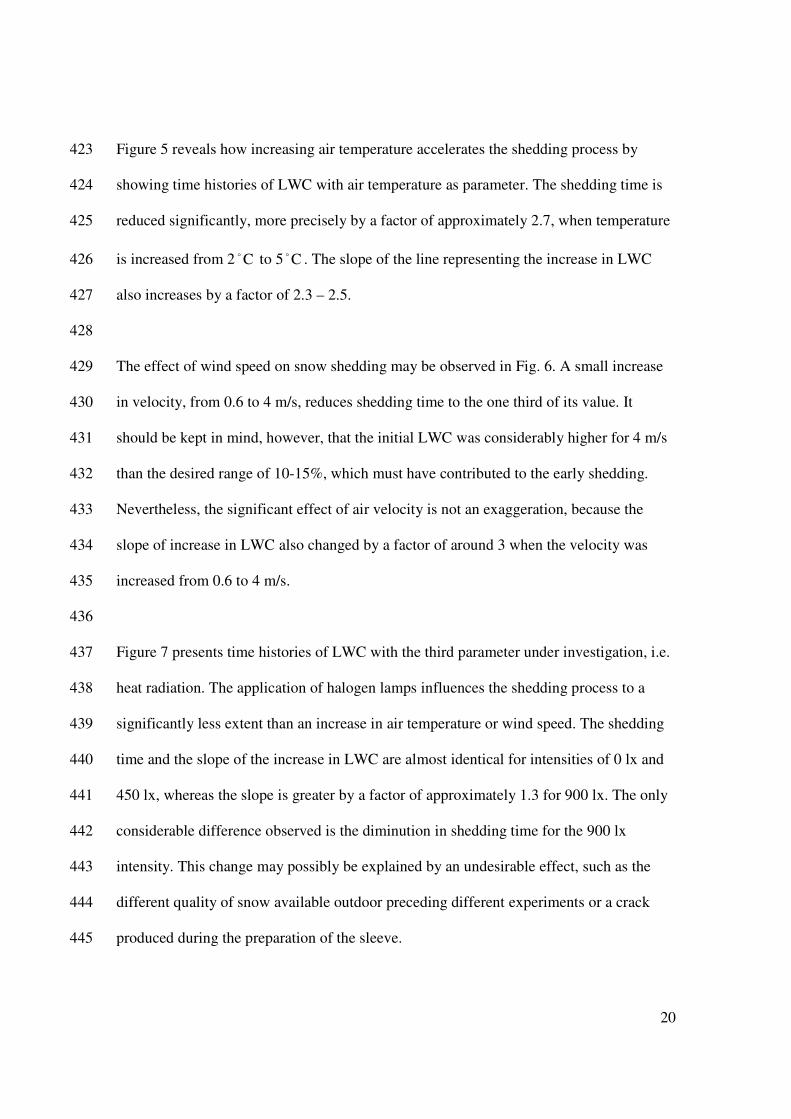
Figure 5 reveals how increasing air temperature accelerates the shedding process by 423
showing time histories of LWC with air temperature as parameter. The shedding time is 424
reduced significantly, more precisely by a factor of approximately 2.7, when temperature 425
is increased from 2 Co to 5 Co . The slope of the line representing the increase in LWC 426
also increases by a factor of 2.3 – 2.5. 427
428
The effect of wind speed on snow shedding may be observed in Fig. 6. A small increase 429
in velocity, from 0.6 to 4 m/s, reduces shedding time to the one third of its value. It 430
should be kept in mind, however, that the initial LWC was considerably higher for 4 m/s 431
than the desired range of 10-15%, which must have contributed to the early shedding. 432
Nevertheless, the significant effect of air velocity is not an exaggeration, because the 433
slope of increase in LWC also changed by a factor of around 3 when the velocity was 434
increased from 0.6 to 4 m/s. 435
436
Figure 7 presents time histories of LWC with the third parameter under investigation, i.e. 437
heat radiation. The application of halogen lamps influences the shedding process to a 438
significantly less extent than an increase in air temperature or wind speed. The shedding 439
time and the slope of the increase in LWC are almost identical for intensities of 0 lx and 440
450 lx, whereas the slope is greater by a factor of approximately 1.3 for 900 lx. The only 441
considerable difference observed is the diminution in shedding time for the 900 lx 442
intensity. This change may possibly be explained by an undesirable effect, such as the 443
different quality of snow available outdoor preceding different experiments or a crack 444
produced during the preparation of the sleeve. 445

21
446
4.3 Comparison of Experimental Observations and Computer Simulations 447
The theoretical model described in Section 3 was applied for several different conditions, 448
and the obtained simulation results were compared to experimental observations. Since 449
the duration of the experiments took several hours, the time step of calculation was 450
chosen to be one minute. Figure 8 shows time histories of LWC as calculated in the entire 451
end section as well as in the top and bottom half of the same section. Measured values of 452
LWC of the snow sleeve are also plotted in this figure. In some of the experiments two 453
samples were taken at each measurement, one from the top and one from the bottom half 454
of the snow sleeve (see Figs. 8c and 8d). The four diagrams in Fig. 8 were chosen to help 455
compare the effects of changing each parameter when the other parameters are not varied. 456
At the beginning of most of the experiments the LWC increases by the same extent 457
everywhere in the snow sleeve, because ice grains start melting, but water percolation is 458
not occurring yet (curves for “simulation, bottom” and “simulation, top” coincide at the 459
beginning in Figs. 8a,c,d and 9). As LWC increases, the water distribution in snow is in 460
funicular mode, water movement toward the bottom of the snow sleeve begins, and the 461
end section starts turning down. Consequently, the LWC increase in the top part slows 462
down, and, at the same time, it accelerates in the bottom part (curves for “simulation, 463
bottom” and “simulation, top” have different slopes and diverge in Figs. 8 and 9). At the 464
end of the experiment, the top part disappears and the LWC in the bottom part 465
approaches the average LWC of the entire section, because the whole section is deflected 466
below the cable (“simulation, bottom” curve approaches “simulation” curve in Figs. 8 467
and 9). It should be noticed that water distribution was in funicular mode even at the 468

22
beginning of the experiment whose simulation results are shown in Fig. 8b. Therefore, 469
the increase in LWC in the top differs from that in the bottom part from the very 470
beginning. Variations in density for the entire section, in the top and the bottom parts are 471
plotted and compared to experimental results for one ambient condition in Fig. 9, where 472
similar tendencies may be observed as for LWC. The difference is that the density does 473
not approach 0 as the LWC does when the mass of snow on the top reduces significantly. 474
In this moment, even a very small amount of water causes a slight increase in the density, 475
since the volume also becomes very small. Although this increase in the density is just a 476
few percent, it was not evaluated as realistic; therefore the density calculated on the top is 477
not presented after this moment. Although the discrepancy between the measured and 478
simulated values is changeable, the increasing tendencies, i.e. the slopes of the curves and 479
the shedding times, are predicted satisfactorily by the model. In the few cases when 480
shedding was delayed by stronger cohesion in the snow, the model is applicable to predict 481
the increase of LWC; however, it fails to estimate shedding time, because the period with 482
approximately constant LWC and with water dripping is not considered. This problem 483
appears to be a challenge in future research. The reader is referred to Olqma, 2009 for 484
further results and details. 485
486
Simulation results are compared to former experimental observations in Fig. 10. The time 487
history of LWC is presented in this figure for the conditions of an experiment carried out 488
by Roberge, 2006. The model provides an acceptable estimation for both of the increase 489
of LWC and the shedding time. The slope of increase of LWC is calculated as 4.4 % / h, 490
and measured as 5.1 % / h; whereas the computed and experimentally obtained shedding 491

23
times are 7h 27min and 6h 38min, respectively. Both discrepancies are within 15%. It 492
should be noted, that the calculated curves in Fig. 10 do not coincide with those in Fig. 493
8a, because the initial conditions (LWC, density) were different. 494
495
The evaluation of different terms in the heat balance makes possible a qualitative 496
comparison between the influences of different heat sources. Table 4 shows the 497
contribution of each heat source when air temperature, wind velocity, and intensity of 498
short-wave radiation are varied. Since the air speed was practically 0.6 m/s in the cases 499
with “no wind” (see Section 2.3), heat flux data are also presented for this velocity. This 500
comparison confirms what was obtained in the experiments: the influence of increasing 501
temperature and wind velocity dominates over the influence of heat radiation. It should 502
be noted, however, that under sunny conditions the heat transfer rate due to short-wave 503
radiation may reach, or even exceed, that due to convection under calm conditions. 504
505
5 Conclusions and Recommendations 506
Wet-snow shedding from a suspended cable with negligible sag under natural conditions 507
has been studied experimentally, and a thermodynamic model has been developed to 508
simulate the variation of LWC and density at the end section of the snow sleeve until 509
shedding. The effects of three parameters were considered: air temperature, wind velocity 510
and solar radiation. Experimental results show that snow shedding under natural 511
conditions begins at the end of the snow sleeve. At the beginning of the shedding process 512
LWC increases in the entire end section, then water starts migrating toward the bottom of 513
sleeve. Eventually, the end section becomes more and more deflected until the snow 514

24
sheds, when external forces exceed adhesive and cohesive forces. Increasing air 515
temperature and wind velocity accelerate this process significantly. The effect of solar 516
radiation is less important when the sky is cloudy though it becomes considerable under 517
sunny conditions. The theoretical model predicts satisfactorily the rate of increase of 518
LWC and the shedding time. The final LWC and final density of the snow when it sheds 519
vary within a considerably wide range. 520
521
The process of snow shedding implies a number of further questions which are out of the 522
scope of the present study, but should be addressed in future research. Some of these 523
topics are as follows: modeling snow shedding from a current-carrying conductor; 524
studying the snow shedding process from a sagged cable; finding the dependence of final 525
LWC and final density on the initial snow characteristics; extending the thermodynamic 526
model to 3D; and defining a shedding condition in terms of external and adhesive forces, 527
which may help to predict rupture in the model of a 3D snow sleeve. 528
529
Acknowledgments 530
This work was carried out within the framework of the NSERC/Hydro-Québec/UQAC 531
Industrial Chair on Atmospheric Icing of Power Network Equipment (CIGELE) and the 532
Canada Research Chair on Engineering of Power Network Atmospheric Icing 533
(INGIVRE) at the Université du Québec à Chicoutimi. The authors would like to thank 534
the CIGELE partners (Hydro-Québec, Hydro One, Électricité de France, Alcan Cable, K-535
Line Insulators, CQRDA and FUQAC) whose financial support made this research 536
possible. 537

25
538
References 539
Admirat, P. and Lapeyre, J.L., 1986. Observation d'accumulation de neige collante à la 540
station de Bagnères de Luchon les 6, 7 avril 1986 - Effet préventif des contrepoids 541
antitorsion, EDF-DER HM/72-5535. 542
Admirat, P., Lapeyre, J.L. and Dalle, B., 1990. Synthesis of Filed Observations and 543
Practical Results of the 1983-1990 "Wet-Snow" Programme of Electricité de 544
France, Proc. of 5th International Workshop on Atmospheric Icing of Structures, 545
Tokyo, Japan, pp. B6-2-(1) - B6-2-(5). 546
Admirat, P., Maccagnan, M. and Goncourt, B.D., 1988. Influence of Joule effect and of 547
climatic conditions on liquid water content of snow accreted on conductors, Proc. 548
of 4th International Workshop on Atmospheric Icing of Structures, Paris, France. 549
Atmospheric Environment Service, 1984. Monthly Radiation Summary, 25. Environment 550
Canada. 551
Bird, R.B., Stewart, W.E. and Lightfoot, E.N., 1960. Transport Phenomena. John Wiley 552
& Sons Inc., New York, NY, USA. 553
Colbeck, S.C., 1972. A Theory of Water Percolation in Snow. Journal of Glaciology, 554
11(63): 369-385. 555
Denoth, A., 1980. The Pendular-Funicular Liquid Transition in Snow. Journal of 556
Glaciology, 25(91): 93-97. 557
Eliasson, A.J. and Thorsteins, E., 2000. Field Measurements of Wet Snow Icing 558
Accumulation, Proc. of 9th International Workshop on Atmospheric Icing of 559
Structures, Chester, England. 560

26
Grenier, J.C., Admirat, P. and Maccagnan, M., 1986. Theoretical Study of the Heat 561
Balance during the Growth of Wet Snow Sleeves on Electrical Conductors, Proc. 562
of 3rd International Workshop on Atmospheric Icing of Structures, Vancouver, 563
BC, Canada, pp. 125-129. 564
Kondratyev, K.Y., 1969. Radiation in the Atmosphere. Academic Press, New York, NY. 565
Makkonen, L., 1984. Modeling of Ice Accretion on Wires. Journal of Climate and 566
Applied Meteorology, 23(6): 929-938. 567
Male, D.H. and Grey, D.M., 1981. Snowcover Ablation and Runoff. In: D.M. Grey and 568
D.H. Male (Editors), Handbook of Snow. Pergamon Press, Toronto, ON. 569
Olqma, O., 2009. Critères de déclenchement du délestage de la neige collante de câbles 570
aériens (Criteria for Initiation of Snow Shedding from Overhead Cables, in 571
French), University of Quebec at Chicoutimi, Chicoutimi, QC, submitted. 572
Poots, G. and Skelton, P.L.I., 1994. Simple models for wet-snow accretion on 573
transmission lines: snow load and liquid water content. International Journal of 574
Heat and Fluid Flow, 15(5): 411-417. 575
Poots, G. and Skelton, P.L.I., 1995. Thermodynamic models of wet-snow accretion: axial 576
growth and liquid water content on a fixed conductor. International Journal of 577
Heat and Fluid Flow, 16(1): 43-49. 578
Roberge, M., 2006. A Study of Wet Snow Shedding from an Overhead Cable. M.Sc. 579
Thesis, McGill University, Montreal, QC. 580
Sakamoto, Y., 2000. Snow accretion on overhead wires. Phil. Trans. R. Soc. Lond. A, 581
358: 2941-2970. 582

27
Sakamoto, Y., Admirat, P., Lapeyre, J.L. and Maccagnan, M., 1988. Thermodynamic 583
simulation of wet snow accretion under wind-tunnel conditions, Proc. of 4th 584
International Workshop on Atmospheric Icing of Structures, Paris, France, pp. 585
Paper A6.6. 586
Sakamoto, Y., Tachizaki, S. and Sudo, N., 2005. Snow Accretion on Overhead Wires, 587
Proc. of 11th International Workshop on Atmospheric Icing of Structures, 588
Montreal, QC, Canada, pp. 3-9. 589
Wakahama, G., Kuroiwa, D. and Goto, K., 1977. Snow Accretion on Electric Wires and 590
its Prevention. Journal of Glaciology, 19(81): 479-487. 591
592
593

28
Tables 594
595
Source of error Precision Parameter affected by source of error
Max error in parameter
Max error in LWC value
Scale on measuring glass
5.0± ml Mass of water, wm 5.0± g 2± %
Digital scale 01.0± g Mass of snow sample,
sm 51.0± g 1± % Handling procedure 5.0± g
Digital thermocouple C5.0 o±
Temperature of hot water, wT C5.0 o± 6± %
Temperature of mixture, mT C5.0 o± 13± %
596
Table 1: Maximum error in the LWC measurement 597
598

29
599 Parameter Symbol Unit Value
Specific heat of air pc ( )KkgJ/ × 1006
Diffusion coefficient of water vapor in air
awD , /sm2 -5102.1×
Thermal conductivity of air ak ( )KmW/ × -2102.42×
Latent heat of fusion fL J/kg 5103.35×
Latent heat of vaporization vL J/kg 6102.5×
Thermal expansion coefficient of air
aβ 1/K ( )( )2//1 sa TT +
Dynamic viscosity of air aµ ( )smkg/ × -5101.73×
Dynamic viscosity of water wµ ( )smkg/ × -3101.79×
Kinematic viscosity of air aν /sm2 -5101.34×
Density of air aρ 3kg/m 1.28
Density of water wρ 3kg/m 1000
Density of ice iρ 3kg/m 917
600
Table 2: Physical parameters describing air, water and ice (temperature dependent 601
parameters are considered at 3 Co ) 602
603

30
604
aT
( Co )
aU
(m/s)
Illumi-nation
(lx)
Initial LWC (%)
Initial density
( 3kg/m )
Final LWC (%)
Final density
( 3kg/m )
Shedding time
(h:min)
Average slope
(% / h)
2 0* 0 29.4 550 45.8 870 (12:00)**
13:00 1.1
3 0 0 12.2 440 40.2 510 (4:00)
7:00 4.8
5 0 0 12.5 460 43.1 730 (6:00)
6:40 4.4
2 2 0 10.0 670 42.5 870 7:00 3.4 3 2 0 15.2 640 50.0 800
(5:00) 6:45 5.9
5 2 0 20.2 540 59.6 850 (3:00)
3:40 10.0
2 4 0 14.2 500 56.8 790 (5:00)
5:30 5.7
3 4 0 12.3 580 46.8 - 3:15 10.1 5 4 0 23.2 580 49.6 640
(1:00) 2:00 13.3
2 0 450 10.0 420 41.9 600 3:25 8.2 3 0 450 8.5 420 43.2 590
(6:10) 7:45 4.5
5 0 450 24.6 590 49.5 0.64 3:10 7.9 2 0 900 9.7 540 44.8 770
(4:00) 7:40 4.6
3 0 900 11.8 520 36.3 0.71 4:00 6.1 5 0 900 16.0 520 47.5 680
(1:00) 2:50 11.2
605
Table 3: Summary of experimental results; * - 0 means “no wind” case, but a velocity of 606
about 0.6 m/s of the circulating air was still measured; ** - time in parentheses below 607
final density data indicates time of last density measurement if it took place earlier than 608
the end of experiment 609
610

31
611 Convective heat flux, cq ( 2W/m )
C2o=aT C3o=aT C5o=aT
0=aU m/s 6 9 15
6.0=aU m/s 21 31 52
2=aU m/s 56 84 140
4=aU m/s 100 149 249
10=aU m/s 213 314 533
(a) 612
Heat flux due to short-wave radiation, srq ,
condition exp, 450 lx exp, 900 lx sunny winter day
srq , ( 2W/m ) 7.5 15 167*
(b) 613
Heat flux due to long-wave radiation, lrq ,
( )CoaT 2 3 5
lrq , ( 2W/m ) 9 14 23
(c) 614
Heat flux due to evaporation / condensation, eq ( 2W/m )
C2o=aT C3o=aT C5o=aT
0=aU m/s -2.3 -0.2 4.5
6.0=aU m/s -8.0 -0.7 15
2=aU m/s -22 -1.9 42
4=aU m/s -39 -3.4 74
10=aU m/s -83 -7.3 159
(d) 615
Table 4: Heat fluxes under different ambient conditions, (a) heat convection, (b) heat due 616
to short-wave radiation considering a snow albedo of 0.6, (c) heat due to long-wave 617
radiation, (d) heat due to evaporation / condensation for a relative humidity of 0.8; * - 618

32
value corresponds to 1.5 ( )hmMJ/ 2 × which is measured at midday on sunny winter days 619
(Atmospheric Environment Service, 1984) 620
621 622

33
Figure Captions 623
Fig. 1: Snow sleeve on the suspended cable at the beginning of an experience using one 624
lamp to simulate heat radiation 625
Fig. 2: Illumination of the snow sleeve by the halogen lamps 626
Fig. 3: Three numerical sub-steps in the ith time step to calculate deflection of end 627
section as well as LWC and density above and below centerline 628
Fig. 4: Evolution of deflection of snow sleeve during the shedding mechanism 629
( C5 o=aT , 2=aU m/s, no radiation), (a) t = 0h; (b) t = 1h; (c) t = 2h; (d) t = 3h 630
Fig. 5: Time histories of LWC until snow shedding with air temperature as parameter; (a) 631
4=aU m/s, no radiation; (b) 900=rI lx, no wind 632
Fig. 6: Time histories of LWC until snow shedding with wind speed as parameter, 633
C5 o=aT , no radiation 634
Fig. 7: Time histories of LWC until snow shedding with heat radiation as parameter, 635
C3 o=aT , no wind 636
Fig. 8: Measured (experiment) and calculated (simulation) LWC time histories, (a) 637
C3o=aT , no wind, no radiation, (b) C3o=aT , 4=aU m/s, no radiation, (c) C2o=aT , 638
4=aU m/s, no radiation, (d) C3o=aT , no wind, 450=rI lx 639
Fig. 9: Measured (experiment) and calculated (simulation) density time histories for 640
C3o=aT , no wind, no radiation 641
Fig. 10: LWC time histories as measured by Roberge, 2006 (experiment) and calculated 642
by the present model (simulation) for C3o=aT , no wind, no radiation 643
644

34
645 646
Fig. 1: Snow sleeve on the suspended cable at the beginning of an experience using one 647 lamp to simulate heat radiation 648
649 650

35
651 652 653
Fig. 2: Illumination of the snow sleeve by the halogen lamps 654 655
halogen lamps
snow sleeve

36
656 657
Fig. 3: Three numerical sub-steps in the ith time step to calculate deflection of end 658 section as well as LWC and density above and below centerline 659
660
i centerline
water flow
R(i+1) (<R(i))
R(i)
y (i)
centerline i+1 i
y(i+1)
a)
b)
c)
∆A(i)

37
661 662
663 664
Fig. 4: Evolution of deflection of snow sleeve during the shedding mechanism 665 ( C5 o=aT , 2=aU m/s, no radiation), (a) t = 0h; (b) t = 1h; (c) t = 2h; (d) t = 3h 666
667

38
668 (a) 669
670
671 672
(b) 673 674
Fig. 5: Time histories of LWC until snow shedding with air temperature as parameter; (a) 675 4=aU m/s, no radiation; (b) 900=rI lx, no wind 676
677

39
678 679
Fig. 6: Time histories of LWC until snow shedding with wind speed as parameter, 680 C5 o=aT , no radiation 681
682
0.6 m/s
2 m/s
4 m/s

40
683 684
Fig. 7: Time histories of LWC until snow shedding with heat radiation as parameter, 685 C3 o=aT , no wind 686
687

41
0
5
10
15
20
25
30
35
40
45
50
0 1 2 3 4 5 6 7 8
Time, h
LW
C,
% experiment
simulation
simulation, bottom
simulation, top
shedding time, exp
shedding time, sim
688 (a) 689
690
0
5
10
15
20
25
30
35
40
45
50
0 0.5 1 1.5 2 2.5 3 3.5
Time, h
LW
C,
% experiment
simulation
simulation, bottom
simulation, top
shedding time, exp
shedding time, sim
691 (b) 692
693 694

42
0
10
20
30
40
50
60
0 1 2 3 4 5 6
Time, h
LW
C,
%
experiment
experiment, bottom
experiment, top
simulation
simulation, bottom
simulation, top
shedding time, exp
shedding time, sim
695 (c) 696
697
0
5
10
15
20
25
30
35
40
45
50
0 2 4 6 8
Time, h
LW
C,
%
experiment
experiment, bottom
experiment, top
simulation
simulation, bottom
simulation, top
shedding time, exp
shedding time, sim
698 (d) 699
700 Fig. 8: Measured (experiment) and calculated (simulation) LWC time histories, (a) 701
C3o=aT , no wind, no radiation, (b) C3o=aT , 4=aU m/s, no radiation, (c) C2o=aT , 702
4=aU m/s, no radiation, (d) C3o=aT , no wind, 450=rI lx 703
704

43
0
100
200
300
400
500
600
0 1 2 3 4 5 6 7
Time, h
Den
sit
y,
kg
/m3
experiment
simulation
simulation, bottom
simulation, top
705 706
Fig. 9: Measured (experiment) and calculated (simulation) density time histories for 707 C3o=aT , no wind, no radiation 708
709

44
0
10
20
30
40
50
60
0 2 4 6 8
Time, h
LW
C,
%
experiment
experiment, bottom
experiment, top
simulation
simulation, bottom
simulation, top
shedding time, exp
shedding time, sim
710 711
Fig. 10: LWC time histories as measured by Roberge, 2006 (experiment) and calculated 712 by the present model (simulation) for C3o=aT , no wind, no radiation 713
714 715