Marga Peeters and Ard den Reijer

On Wage Formation, Wage

Development and Flexibility:

A comparison between European

countries and the United States

No. 108/2003

On Wage Formation, Wage Development and Flexibility:A comparison between European countries and the United States

Marga Peeters and Ard den Reijer

DNB Staff Reports 2003, No. 108

De Nederlandsche Bank

©2003 De Nederlandsche Bank NV

Corresponding author: Marga Peeters

e-mail: h.m.m.peeters@dnb.nl

Aim and scope of DNB Staff Reports are to disseminate research done by

staff members of the Bank to encourage scholarly discussion.

Views expressed are those of the individual authors and do not necessarily

reflect official positions of the Nederlandsche Bank.

Editorial Committee

Peter van Els (chairman), Eelco van den Berg (secretary), Hans Brits, Maria Demertzis, Maarten

Gelderman, Jos Jansen, Klaas Knot, Peter Koeze, Marga Peeters, Bram Scholten, Job Swank.

Subscription orders for DNB Staff Reports and requests for specimen copies

should be sent to:

De Nederlandsche Bank NV

Communication and Information Department

Westeinde 1

P.O. Box 98

1000 AB Amsterdam

The Netherlands

Internet: www.dnb.nl

1

ON WAGE FORMATION, WAGE DEVELOPMENT AND FLEXIBILITY:

a comparison between European countries and the United States *

Marga Peeters and Ard den Reijer **

October, 2003

Abstract

For Germany, Spain, France, the Netherlands and the US an Error Correction Model with a

long-term non-linear wage equation is estimated by 3-SLS to obtain consistent estimates,

accounting for endogeneity and common shocks. On the basis of the estimated parameter

elasticities of wages with respect to labour productivity, value added and consumer prices, taxes,

unemployment and replacement rates are computed along with the wage contributions. The

results indicate that the dominant role of prices in the formation of wages in the seventies and

eighties was taken over by labour productivity in the US and unemployment in Spain and –

almost- in the Netherlands at the end of the nineties. Evidence for a stronger real wage flexibility

of the US in comparison with the four European countries is not found.

JEL codes: C22, E24, J30.

Key words: wage fexibility, labour market.

* This paper is a follow up of the WO&E Research Memorandum On wage formation, wage

development and unemployment no. 677 by the same authors that appeared in 2001. Extensions

and improvements in this paper concern (1) the application of the econometric model to

Germany, France and the United States in addition to –what was done in the previous version-

Spain and the Netherlands (2) one additional degree of freedom in the theoretical model by

allowing for a non-unity elasticity of the labour productivity in the wage equation and (3) the

estimation strategy, being a system 3-Stage-Least-Squares procedure instead of univariate

Ordinary Least Squares. It is further a revised version of WO Research Memorandum no. 712.

** The authors are very grateful for the comments of two anonymous referees and participants, in

particular Esther Moral, during seminars at the Nederlandsche Bank, the European Central Bank

and the Banque de France. Moreover, we would like to thank Lex Hoogduin and Peter van Els for

useful comments. We would further like to thank Menno Grevelink, Sybille Grob and Peter Keus

for statistical assistance. All errors remain ours.

2

1 INTRODUCTION

This study goes into the complexity of wage formation. The aim is to study wage developments,

wage formation and wage flexibility for a number of European countries in comparison with the

US. Considering the labour market changes that took place in the nineties in Spain and the

Netherlands and also in the US, wage formation seems to have changed considerably during the

last decade. We study here in particular wage developments in order to illuminate the differences

across European countries, but also with the United States.

We adopt a theoretical model where a non-linear wage equation can be derived, as developed

by Graafland and Huizinga (1999) and also used in Peeters and Den Reijer (2001). One main

difference of the model used here is that no longer a unity elasticity of wages with respect to

labour productivity. A second difference is that this model is estimated for Germany, Spain,

France, the Netherlands and the United States and the accompanying elasticities are calculated

whereas Graafland and Huizinga estimated the model for the Netherlands only. As a third

difference, special attention is paid to the estimation strategy in order to have a solid framework

for the deduction of (policy) conclusions. The theoretical model is fully consistent with the

empirical analyses. To the best of our knowledge no other studies exist where the here presented

wage bargaining model is used or with a strong coherence between theoretical and empirical

results on wage bargaining.

The non-linear nature of the wage equation derived has the advantage that the elasticities of

wages need not necessarily be constant. So, instead of the constant elasticities presented in other

studies like Layard et al. (1991), this framework enables us to compute elasticities that can differ

over time. Moreover, we are able to quantify the partial contributions of the different

determinants to the wage increase. These calculations are presented during almost thirty years.

The determinants that turn out to be dominant during the three different decades will be

investigated. Furthermore, not only flexibility in the long term, but also wage flexibility in the

short term, real as well as nominal, gains a prominent place in this study.

The organisation of this paper is as follows. Section 2 presents the theoretical model and the

derivation of the non-linear wage equation. Section 3 discusses the main wage determinants

according to this model. Section 4 to 7 report the estimation results. In section 4 the estimated

wage equations for the countries are presented. Section 5 presents the elasticities, section 6 the

contributions of the determinants to wage formation and Section 7 pays attention to real and

nominal wage flexibility. Section 8 summarises and concludes.

3

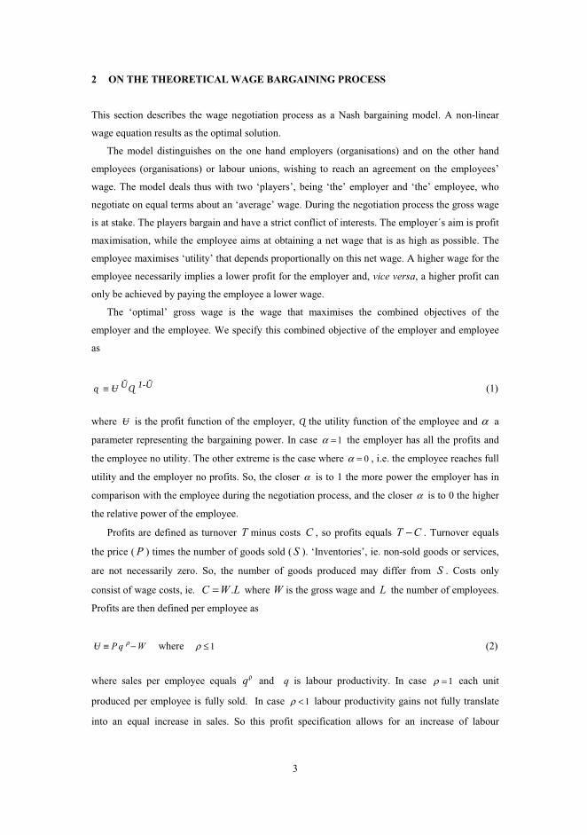
2 ON THE THEORETICAL WAGE BARGAINING PROCESS

This section describes the wage negotiation process as a Nash bargaining model. A non-linear

wage equation results as the optimal solution.

The model distinguishes on the one hand employers (organisations) and on the other hand

employees (organisations) or labour unions, wishing to reach an agreement on the employees’

wage. The model deals thus with two ‘players’, being ‘the’ employer and ‘the’ employee, who

negotiate on equal terms about an ‘average’ wage. During the negotiation process the gross wage

is at stake. The players bargain and have a strict conflict of interests. The employer´s aim is profit

maximisation, while the employee aims at obtaining a net wage that is as high as possible. The

employee maximises ‘utility’ that depends proportionally on this net wage. A higher wage for the

employee necessarily implies a lower profit for the employer and, vice versa, a higher profit can

only be achieved by paying the employee a lower wage.

The ‘optimal’ gross wage is the wage that maximises the combined objectives of the

employer and the employee. We specify this combined objective of the employer and employee

as

Ŭ 1-Ŭɋ Ʉ Ɋ≡ (1)

where Ʉ is the profit function of the employer, Ɋ the utility function of the employee and α a

parameter representing the bargaining power. In case 1α = the employer has all the profits and

the employee no utility. The other extreme is the case where 0α = , i.e. the employee reaches full

utility and the employer no profits. So, the closer α is to 1 the more power the employer has in

comparison with the employee during the negotiation process, and the closer α is to 0 the higher

the relative power of the employee.

Profits are defined as turnover T minus costs C , so profits equals T C− . Turnover equals

the price ( P ) times the number of goods sold ( S ). ‘Inventories’, ie. non-sold goods or services,

are not necessarily zero. So, the number of goods produced may differ from S . Costs only

consist of wage costs, ie. .C W L= where W is the gross wage and L the number of employees.

Profits are then defined per employee as

Ʉ P q Wρ≡ − where 1ρ ≤ (2)

where sales per employee equals qρ and q is labour productivity. In case 1ρ = each unit

produced per employee is fully sold. In case 1ρ < labour productivity gains not fully translate

into an equal increase in sales. So this profit specification allows for an increase of labour

4

productivity that is not necessarily fully translated in a proportional increase in sales. In case

1ρ < profit is lower due to the lower revenues per employee, but higher as a consequence of the

lower gross wage as becomes clear from equation (7). See also Bell, Nickell en Quintini (2000)

for a similar specification.

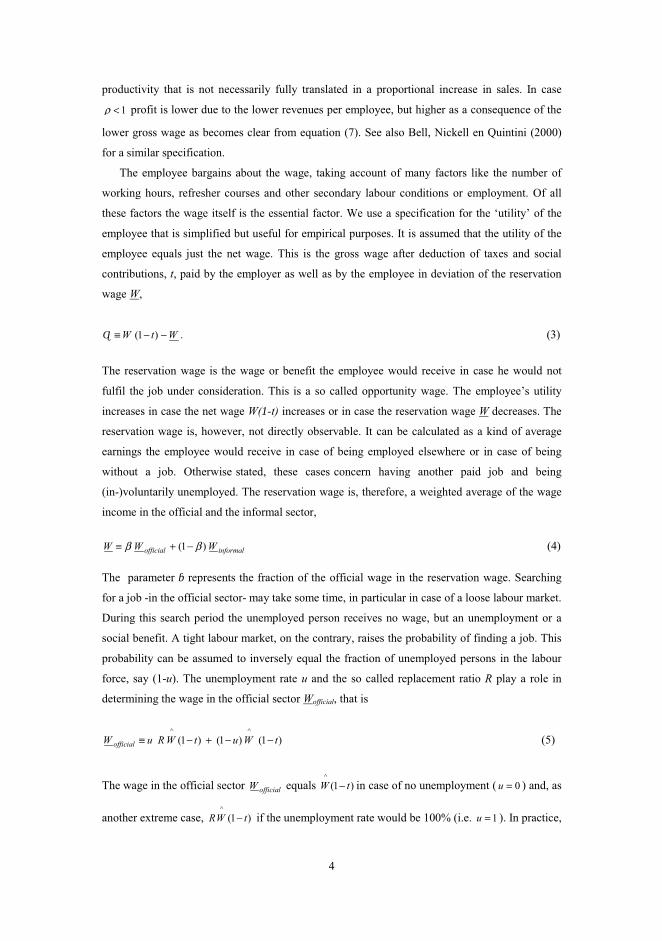
The employee bargains about the wage, taking account of many factors like the number of

working hours, refresher courses and other secondary labour conditions or employment. Of all

these factors the wage itself is the essential factor. We use a specification for the ‘utility’ of the

employee that is simplified but useful for empirical purposes. It is assumed that the utility of the

employee equals just the net wage. This is the gross wage after deduction of taxes and social

contributions, t, paid by the employer as well as by the employee in deviation of the reservation

wage W,

(1 )Ɋ W t W≡ − − . (3)

The reservation wage is the wage or benefit the employee would receive in case he would not

fulfil the job under consideration. This is a so called opportunity wage. The employee’s utility

increases in case the net wage W(1-t) increases or in case the reservation wage W decreases. The

reservation wage is, however, not directly observable. It can be calculated as a kind of average

earnings the employee would receive in case of being employed elsewhere or in case of being

without a job. Otherwise stated, these cases concern having another paid job and being

(in-)voluntarily unemployed. The reservation wage is, therefore, a weighted average of the wage

income in the official and the informal sector,

(1 )official informalW W Wβ β≡ + − (4)

The parameter ɓ represents the fraction of the official wage in the reservation wage. Searching

for a job -in the official sector- may take some time, in particular in case of a loose labour market.

During this search period the unemployed person receives no wage, but an unemployment or a

social benefit. A tight labour market, on the contrary, raises the probability of finding a job. This

probability can be assumed to inversely equal the fraction of unemployed persons in the labour

force, say (1-u). The unemployment rate u and the so called replacement ratio R play a role in

determining the wage in the official sector Wofficial, that is

^ ^

(1 ) (1 ) (1 )officialW u R W t u W t≡ − + − − (5)

The wage in the official sector officialW equals ^

(1 )W t− in case of no unemployment ( 0u = ) and, as

another extreme case, ^

(1 )RW t− if the unemployment rate would be 100% (i.e. 1u = ). In practice,

5

the wage in the official sector will be somewhere in between these two extremes. Wage ^

W is the

gross average ‘market’ wage. The gross benefit received when unemployed equals ^

R W as the

replacement rate R equals the ‘average’ unemployment benefit divided by the average market

wage. This replacement rate plays an important part in this model. It can be seen as a sort of

reduction in income in case a person, in comparison with his wage income when being at work,

does not work.

The wage obtained in the unofficial sector can result from work done in the black market or

saved expenditures due to homework. Examples of the latter are savings due to child care,

cleaning or house (re-) decoration. It is assumed that productivity in the informal sector is linked

to that of the official sector because of spillovers of technological progress improving labour

productivity in general. A parameter γ allows for a relatively low labour productivity of the

informal vis-à-vis the official sector. Earnings in the informal sector consisting of savings and/or

expenses, represented as Winformal, is further assumed conditional on the consumer price Pc,

.cinformalW P qργ≡ (6)

So the real wage earned in the informal sector, informal

c

W

P is lower than or equal to the productivity

in the formal sector in case 1γ ≤ and 1ρ = (see (2)). In case 1ρ < some ‘goods’ produced do

not raise money at all.

It is sometimes argued that the ‘informal’ sector does hardly or does not exist. In this case

parameter ɓ should equal one (see (4)). In our empirical analyses we test this restriction.

Appendix A shows that the wage equation resulting from this bargaining process reads as

( )( ) ( )

( )( ) ( )

1log log log log 1 1

1 1 1

1log 1 1 1 1 log 1

1 1

cPW P q

P t

u R

α β γρ

α α β γ

α β γα βα α

−= + + + − − + − −

− − + − − − + + − −

(7)

From this wage equation it follows that prices fully translate in gross wage increases. A 1%

increase in the value added price and the consumer price, increases the gross wage by 1%.

Productivity does not necessarily translate fully in wage increases. In case productivity increase

by 1%, gross wage increase by ρ, where ρ is not necessarily equal to 1. In case 1ρ < the

employee receives less wage than in case 1ρ = and at the same time the employer pays less due

to lower wage costs. Due to a lower turnover the employer may even not benefit much from the

6

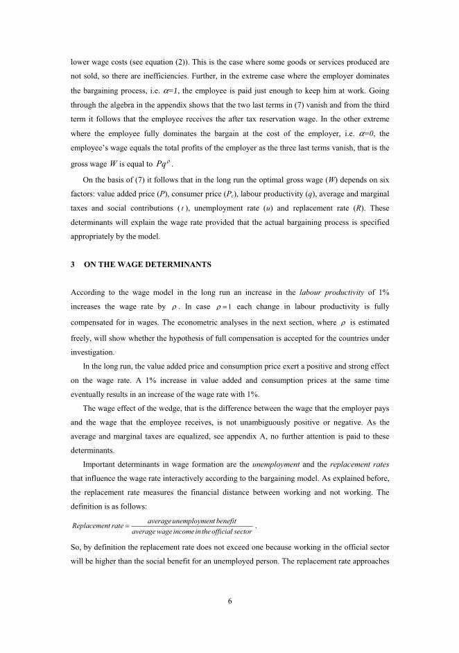
lower wage costs (see equation (2)). This is the case where some goods or services produced are

not sold, so there are inefficiencies. Further, in the extreme case where the employer dominates

the bargaining process, i.e. α=1, the employee is paid just enough to keep him at work. Going

through the algebra in the appendix shows that the two last terms in (7) vanish and from the third

term it follows that the employee receives the after tax reservation wage. In the other extreme

where the employee fully dominates the bargain at the cost of the employer, i.e. α=0, the

employee’s wage equals the total profits of the employer as the three last terms vanish, that is the

gross wage W is equal to Pqρ.

On the basis of (7) it follows that in the long run the optimal gross wage (W) depends on six

factors: value added price (P), consumer price (Pc), labour productivity (q), average and marginal

taxes and social contributions ( t ), unemployment rate (u) and replacement rate (R). These

determinants will explain the wage rate provided that the actual bargaining process is specified

appropriately by the model.

3 ON THE WAGE DETERMINANTS

According to the wage model in the long run an increase in the labour productivity of 1%

increases the wage rate by ρ . In case 1ρ = each change in labour productivity is fully

compensated for in wages. The econometric analyses in the next section, where ρ is estimated

freely, will show whether the hypothesis of full compensation is accepted for the countries under

investigation.

In the long run, the value added price and consumption price exert a positive and strong effect

on the wage rate. A 1% increase in value added and consumption prices at the same time

eventually results in an increase of the wage rate with 1%.

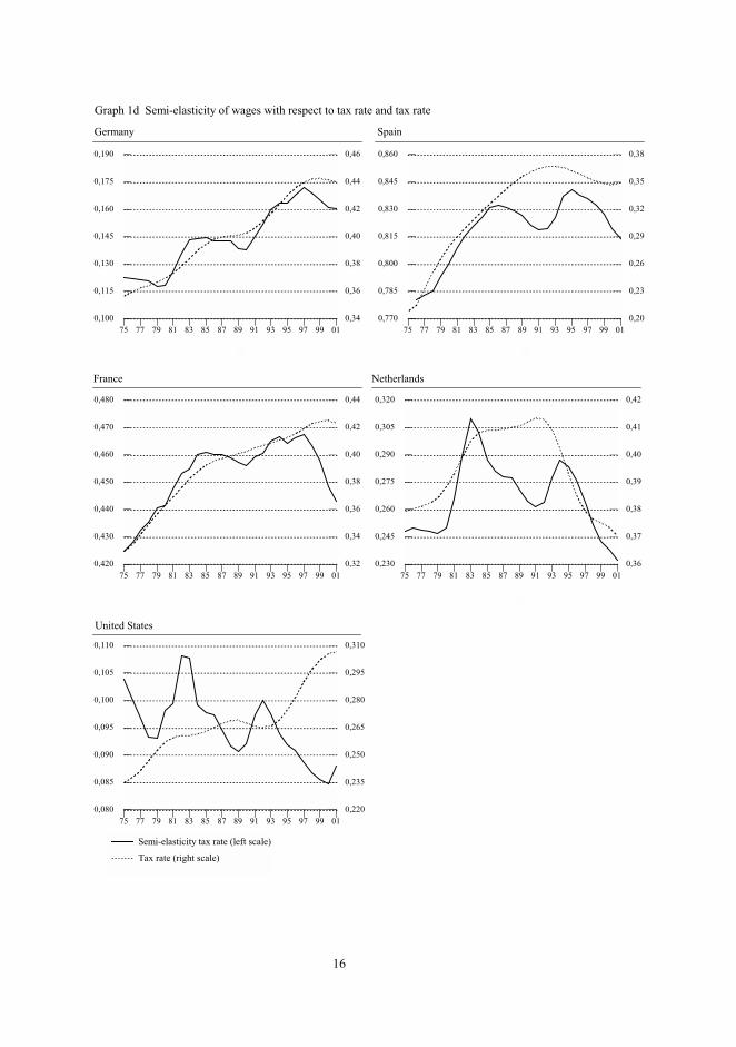
The wage effect of the wedge, that is the difference between the wage that the employer pays

and the wage that the employee receives, is not unambiguously positive or negative. As the

average and marginal taxes are equalized, see appendix A, no further attention is paid to these

determinants.

Important determinants in wage formation are the unemployment and the replacement rates

that influence the wage rate interactively according to the bargaining model. As explained before,

the replacement rate measures the financial distance between working and not working. The

definition is as follows:

averageunemployment benefitReplacement rate

average wageincomein theofficial sector= .

So, by definition the replacement rate does not exceed one because working in the official sector

will be higher than the social benefit for an unemployed person. The replacement rate approaches

7

one if the financial distance between working and not working becomes smaller. It is close to

zero if the earned wage in the official sector is high in comparison with the unemployment

benefit.

Empirical evidence also shows that the replacement rate affects the wage rate positively. The

case of an increasing replacement rate, so a smaller distance between working and not working,

will put upward pressure on the wage rate in the long term. The wage rate has to compensate for

the difference between both situations. The smaller the distance, the larger the wage

compensation. In the extreme case where the distance is zero, i.e. the replacement rate is equal to

one, the employee has no financial incentive to work. He will require a wage compensation

before taking part in the paid labour process. A tight (loose) labour market will increase

(decrease) the denominator of the replacement rate. Shortage (abundance) of the work force is

expected to exert more (less) pressure on the wage rate. This pressure will raise (lower) the

average wage in the economy. The numerator of the replacement rate on the other hand

experiences more influence from changes in social security, like unemployment benefits, other

social security payments, taxes, social contributions, and so on.

A higher unemployment rate leads, as one may expect because of the higher demand for than

supply of paid jobs, to downward pressure on the wage rate. The effect of the unemployment rate

on the wage rate is thus negative. The magnitude of this effect depends on the replacement rate.

The unemployment rate moderates the wage rate most when unemployment is high and the

replacement rate low. This situation is a combination of a loose labour market while at the same

time working is much more profitable than not working. In this situation many people are

involuntarily unemployed. The wage moderating effect of unemployment will be higher as long

as not working is less remunerative. In times of a relatively high replacement rate that is almost

equal to one, the difference between remuneration in case of working as compared to non-

working is by definition small. The replacement rate itself exerts a positive effect on the wage

rate. The reservation wage increases, which causes the employee to require a higher wage claim

in order to achieve his optimal level of utility. As stated earlier, the effect on the wage rate at the

same time depends on the unemployment rate. So the unemployment and replacement rate

interactively affect wages.

The specified wage bargaining model aims to describe wage formation appropriately. The

special feature of the resulting wage equation concerns the non-linear character. As a

consequence, a 1 percentage point change in, for example, the unemployment rate affects the

wage rate not necessarily to the same extent at different points in time. Wage ‘flexibility’ may

change over time. These partial effects or elasticities are calculated for all six determinants for a

certain sample based on estimated parameters that appear in the model. These are presented and

discussed in the next section.

8

One important remark is finally to be made concerning the model. Institutional changes and

government regulation affecting the labour market can exert influence on the bargaining process.

The model only accounts for these changes to the extent that they appear in the replacement rate.

4 ON THE ESTIMATION OF THE WAGE EQUATION

This section presents details on the estimation strategy in subsection 4.1 and the estimation results

in subsection 4.2. For those readers not interested in the technical details of the estimation

strategy section 4.1 can be skipped.

4.1 Estimation strategy

The derived result (7) for the gross wage rate can be considered a long-term Nash equilibrium. In

the short run the gross wage may deviate from this equilibrium wage. For this reason an Error

Correction Model (ECM) is specified as

( )*1 1log log log logi iW X W Wφ η − −∆ = ∆ + − . (8)

where log *W equals the highly non-linear right hand side of equation (7) at time 1t − , with the

deep parameters , ,α β γ and ρ . The first terms in (8) consider the short-term effects iφ of the

explanatory variables iX .

The wage equation (8) is estimated for Germany, Spain, France, the Netherlands and the

United States with annual data for the period 1970-2001. Test statistics show that endogeneity

problems arise as the domestic consumer and value added price cp and p -that are highly

significant in the short term- are influenced by the variable to be explained, i.e. the domestic

nominal wage. For this reason instruments are used to obtain consistent estimates. The

instruments taken in the analyses are three and four year lagged exogenous variables of the own

country, in addition to three and four quarter lagged US consumer prices for each of the European

countries. Vice versa, next to the three to four quarter lagged US variables, three and four quarter

lagged German consumer prices are used as instruments in the US equation. The inclusion of the

lagged instruments enforces us to drop the first five observations so that the estimation sample

period is 1975-2001.

The deep parameters resulting from the theoretical model are estimated directly, so all non-

linear restrictions according to (7) are imposed in the long-run relationship for each of the

countries. The identification of both the parameters β and γ turns out to be difficult. For this

reason we calibrate β , being the fraction of the official to average wage (i.e. official wage in the

9

informal sector), at a value between 0.85 and 0.99 that provides the highest t -value of γ . In

order to specify the short term dynamics we start with a general to specific approach with all six

explanatory variables included with no, one and two lags. Variables that turn out not to be

significant at the 5%-level are dropped so that a more specific model remains.

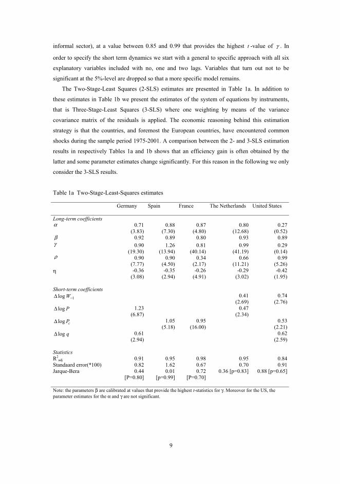
The Two-Stage-Least Squares (2-SLS) estimates are presented in Table 1a. In addition to

these estimates in Table 1b we present the estimates of the system of equations by instruments,

that is Three-Stage-Least Squares (3-SLS) where one weighting by means of the variance

covariance matrix of the residuals is applied. The economic reasoning behind this estimation

strategy is that the countries, and foremost the European countries, have encountered common

shocks during the sample period 1975-2001. A comparison between the 2- and 3-SLS estimation

results in respectively Tables 1a and 1b shows that an efficiency gain is often obtained by the

latter and some parameter estimates change significantly. For this reason in the following we only

consider the 3-SLS results.

Table 1a Two-Stage-Least-Squares estimates

Germany Spain France The Netherlands United States

Long-term coefficientsα 0.71

(3.83)

0.88

(7.30)

0.87

(4.80)

0.80

(12.68)

0.27

(0.52)

β 0.92 0.89 0.80 0.93 0.89

γ 0.90

(19.30)

1.26

(13.94)

0.81

(40.14)

0.99

(41.19)

0.29

(0.14)ρ 0.90

(7.77)

0.90

(4.50)

0.34

(2.17)

0.66

(11.21)

0.99

(5.26)

η -0.36

(3.08)

-0.35

(2.94)

-0.26

(4.91)

-0.29

(3.02)

-0.42

(1.95)

Short-term coefficients

1log W−∆ 0.41

(2.69)

0.74

(2.76)

log P∆ 1.23

(6.87)

0.47

(2.34)

log cP∆ 1.05

(5.18)

0.95

(16.00)

0.53

(2.21)

log q∆ 0.61

(2.94)

0.62

(2.59)

Statistics

R2

adj 0.91 0.95 0.98 0.95 0.84

Standaard error(*100) 0.82 1.62 0.67 0.70 0.91

Jarque-Bera 0.44

[P=0.80]

0.01

[p=0.99]

0.72

[P=0.70]

0.36 [p=0.83] 0.88 [p=0.65]

Note: the parameters β are calibrated at values that provide the highest t-statistics for γ. Moreover for the US, the

parameter estimates for the α and γ are not significant.

10

Table 1b Three-Stage-Least-Squares-estimates

Germany Spain France The Netherlands United States

Long-term coefficientsα 0.58

(2.44)

0.95

(13.94)

0.76

(3.10)

0.77

(9.34)

0.40

(0.93)

β 0.92 0.83 0.80 0.92 0.89

γ 0.83

(8.04)

0.98

(19.16)

0.83

(28.67)

0.95

(31.13)

0.68

(0.96)ρ 0.88

(10.94)

0.94

(5.41)

0.38

(2.27)

0.67

(9.31)

0.93

(4.53)η -0.38

(3.59)

-0.36

(3.44)

-0.29

(3.70)

-0.32

(3.12)

-0.39

(2.15)

Short-term coefficients

1log W−∆ 0.26

(1.99)

0.40

(3.48)

0.63

(3.60)

log P∆ 1.38

(8.26)

0.52

(3.25)

log cP∆ 0.88

(3.96)

0.95

(10.50)

0.55

(2.52)

log q∆ 0.64

(4.43)

0.74

(2.79)

Statistics

R2

adj 0.90 0.96 0.98 0.95 0.84

Standaard error(*100) 0.84 1.42 0.71 0.69 0.88

Jarque-Bera 0.58

[P=0.75]

0.05

[P=0.97]

0.40

[P=0.82]

0.22 [P=0.89] 0.85 [P=0.65]

Note: the parameters β are calibrated at values that provide the highest t-statistics for γ. Moreover for the US, the

parameter estimates for the α and γ are not significant.

One drastic step could further be made by assuming wage co-ordination across countries, or

assuming that some countries in their domestic wage negotiations take account of developments

in e.g. inflation of a neighbouring country.1 Considering the significant differences in parameter

estimates across countries, this step has deliberately not been taken. So, no cross-equation

parameter restrictions are imposed.

Neither are any parameters restricted to predetermined values. Our interest concerns the

impact on wages of the determinants as provided by the wage bargaining model and the data.

These estimation results therefore give us the opportunity to study each of the estimated

determinants' impact in full depth.

1 Belgium would be an appropriate example (but is not included in the sample) of such a case. Wage negotiations

in Belgium are dominantly determined by wage settlements in France, Germany and the Netherlands.

11

4.2 The estimation results

The estimated equations all have a high goodness-of-fit from about 0.84 for the US up to 0.98 for

France. All parameter estimates are used in the next sections where the wage elasticities and

determinants’ contributions to wage growth are discussed. A few remarks have to be made here.

A remarkable finding is the quite high short-term elasticities of prices in Germany (of more than

1%). Moreover, the labour productivity in France and the Netherlands contributes significantly

less than fully to wage growth in the long run. In particular in France the parameter estimate of

ρ is very low, implying that despite higher productivity goods or probably many services are not

sold. Further, and probably most remarkable, is the fact that in the US neither α nor γ are

significant. It seems that neither the unemployment nor the replacement rate is relevant for the

formation of the US wage. As follows from equations (1)-(3) this result implies that wage

negotiations in European countries are much more dominated by employers than in the US.

Moreover, the informal sector in the US is far less important than the informal sector in the

European countries probably due tot the differences in social security arangements across the two

continents.

5 ON THE CALCULATED WAGE ELASTICITIES

For each of the determinants in the wage equation elasticities are calculated and shown in

Graph1a to Graph 1f along with the determinants. The precise formulas for the long-run

elasticities are provided in appendix A.

The elasticity of wages with respect to labour productivity is constant. As follows directly

from Table 1b by means of the estimate for ρ , Graph 1a shows that this elasticity is low for

France and the Netherlands while this parameter is not significantly different to 1 for some other

countries. In case of the Netherlands the low spillover of productivity growth into wages during

the last 25 years may reflect the policy of wage moderation pursued during most of this period. In

the Wassenaar treaty of 1982 employers and employees agreed on full price compensation and on

partially transmission of productivity improvements into wage increases. However, the fairly low

value of ρ for France remains puzzling. The development of the labour productivity in the US

turns out to have increased considerably at the end of the nineties. Spain, on the other hand,

shows a slow-down. We emphasize further that the findings of ρ lower than 1 for some

countries justifies equation (7) where this parameter allows for the empirical flexibility of not

translating productivity changes one-to-one in wages, like confirmed by many empirical studies

that estimate unrestricted form wage equations. In the structural model used here, equation (2) is

the underlying source of the justification.

12

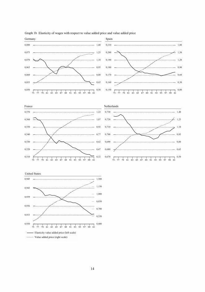
Graphs 1b and 1c provide the elasticities of wages with respect to the two prices, the value

added and consumer price. For each point in time they add up to one by definition, for each of the

countries. It follows that the consumer price elasticity increased over time, at the cost of the value

added price one. At the end of the period, however, for some countries the size of the elasticity

diminishes. According to these estimates the reaction of wage growth to the consumer price is

highest in Spain and lowest in the US.

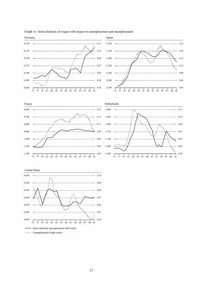
Most interesting cases are the unemployment and the replacement rates. The semi-elasticities

are plotted in Graphs 1e and 1f. On average the semi-elasticity of wages with respect to

unemployment is highest in Spain and the Netherlands and lowest in the US. Interesting is

furthermore that Graph 1f clearly shows that at the end of 20th century the elasticity increased –in

absolute terms- in the Netherlands and Spain, along with the fall in the unemployment rate. In

Germany, on the other hand, the responsiveness of the wage rate to unemployment was fairly low

and lowered even further during the end of the sample period. In France the responsiveness of

wage growth to unemployment was –in absolute terms- also relatively low, but diminished a little

at the very end of the period. At this point we want to stress that the semi-elasticity of wages with

respect to unemployment is dependent upon the unemployment rate itself, the replacement rate

and the deep parameters α and β (see (A.4) in appendix A). As follows from the strong

similarity of the development of the calculated unemployment elasticities in Graph 1e and the

replacement rates as given in Graph 1f the dominance of the replacement rate is apparent. So, for

this reason, we can argue that the decrease in the replacement rate at the end of the nineties as a

consequence of a higher average wage rate and probably a relatively lower unemployment benefit

contributed to the higher flexibility of wages. The high replacement rate in Germany, in contrast,

lowered the flexibility of the German wage. More information about labour market policy

affecting the replacement rate in the countries under investigation here is found in Peeters and

Den Reijer (2001).

The low responsiveness of wages to unemployment in the US might be rationalised by the

functioning of its labour market. The US labour market likely moves towards equilibrium more

by quantity adjustments than by wage adjustments. Because of the loose job protection measures

for employees firms more easily dismiss people when they are no longer sufficiently productive.

As will be shown shortly, the labour productivity turns out to be a dominant contributer to wages

in the US.

13

75 77 79 81 83 85 87 89 91 93 95 97 99 01

0,860

0,865

0,870

0,875

0,880

0,885

0,890

0,60

0,70

0,80

0,90

1,00

1,10

1,20

Graph 1a Elasticity of wages with respect to labour productivity and labour productivity

Germany Spain

75 77 79 81 83 85 87 89 91 93 95 97 99 01

0,930

0,935

0,940

0,945

0,950

0,955

0,960

0,60

0,70

0,80

0,90

1,00

1,10

1,20

75 77 79 81 83 85 87 89 91 93 95 97 99 01

0,360

0,365

0,370

0,375

0,380

0,385

0,390

0,60

0,70

0,80

0,90

1,00

1,10

France

75 77 79 81 83 85 87 89 91 93 95 97 99 01

0,650

0,655

0,660

0,665

0,670

0,675

0,680

0,60

0,70

0,80

0,90

1,00

1,10

1,20

Netherlands

75 77 79 81 83 85 87 89 91 93 95 97 99 01

0,910

0,915

0,920

0,925

0,930

0,935

0,940

0,700

0,800

0,900

1,000

1,100

1,200

1,300

Elasticity labour productivity (left scale)

Labour productivity (right scale)

United States

14

75 77 79 81 83 85 87 89 91 93 95 97 99 01

0,850

0,855

0,860

0,865

0,870

0,875

0,880

0,50

0,65

0,80

0,95

1,10

1,25

1,40

Graph 1b Elasticity of wages with respect to value added price and value added price

Germany Spain

75 77 79 81 83 85 87 89 91 93 95 97 99 01

0,150

0,160

0,170

0,180

0,190

0,200

0,210

0,00

0,30

0,60

0,90

1,20

1,50

1,80

75 77 79 81 83 85 87 89 91 93 95 97 99 01

0,510

0,520

0,530

0,540

0,550

0,560

0,570

0,32

0,47

0,62

0,77

0,92

1,07

1,22

France

75 77 79 81 83 85 87 89 91 93 95 97 99 01

0,670

0,680

0,690

0,700

0,710

0,720

0,730

0,50

0,65

0,80

0,95

1,10

1,25

1,40

Netherlands

75 77 79 81 83 85 87 89 91 93 95 97 99 01

0,930

0,933

0,936

0,939

0,942

0,945

0,400

0,550

0,700

0,850

1,000

1,150

1,300

Elasticity value added price (left scale)

Value added price (right scale)

United States

15

75 77 79 81 83 85 87 89 91 93 95 97 99 01

0,120

0,125

0,130

0,135

0,140

0,145

0,150

0,50

0,65

0,80

0,95

1,10

1,25

1,40

Graph 1c Elasticity of wages with respect to consumer price and consumer price

Germany Spain

75 77 79 81 83 85 87 89 91 93 95 97 99 01

0,780

0,790

0,800

0,810

0,820

0,830

0,840

0,00

0,30

0,60

0,90

1,20

1,50

1,80

75 77 79 81 83 85 87 89 91 93 95 97 99 01

0,430

0,440

0,450

0,460

0,470

0,480

0,490

0,32

0,47

0,62

0,77

0,92

1,07

1,22

France

75 77 79 81 83 85 87 89 91 93 95 97 99 01

0,260

0,270

0,280

0,290

0,300

0,310

0,320

0,50

0,65

0,80

0,95

1,10

1,25

1,40

Netherlands

75 77 79 81 83 85 87 89 91 93 95 97 99 01

0,400

0,550

0,700

0,850

1,000

1,150

1,300

0,056

0,058

0,060

0,062

0,064

0,066

0,068

Elasticity consumer price (left scale)

Consumer price (right scale)

United States

16

75 77 79 81 83 85 87 89 91 93 95 97 99 01

0,100

0,115

0,130

0,145

0,160

0,175

0,190

0,34

0,36

0,38

0,40

0,42

0,44

0,46

Graph 1d Semi-elasticity of wages with respect to tax rate and tax rate

Germany Spain

75 77 79 81 83 85 87 89 91 93 95 97 99 01

0,770

0,785

0,800

0,815

0,830

0,845

0,860

0,20

0,23

0,26

0,29

0,32

0,35

0,38

75 77 79 81 83 85 87 89 91 93 95 97 99 01

0,420

0,430

0,440

0,450

0,460

0,470

0,480

0,32

0,34

0,36

0,38

0,40

0,42

0,44

France

75 77 79 81 83 85 87 89 91 93 95 97 99 01

0,230

0,245

0,260

0,275

0,290

0,305

0,320

0,36

0,37

0,38

0,39

0,40

0,41

0,42

Netherlands

75 77 79 81 83 85 87 89 91 93 95 97 99 01

0,080

0,085

0,090

0,095

0,100

0,105

0,110

0,220

0,235

0,250

0,265

0,280

0,295

0,310

Semi-elasticity tax rate (left scale)

Tax rate (right scale)

United States

17

75 77 79 81 83 85 87 89 91 93 95 97 99 01

-0,820

-0,805

-0,790

-0,775

-0,760

-0,745

-0,730

0,02

0,04

0,05

0,07

0,08

0,10

0,11

Graph 1e Semi-elasticity of wages with respect to unemployment and unemployment

Germany Spain

75 77 79 81 83 85 87 89 91 93 95 97 99 01

-2,700

-2,500

-2,300

-2,100

-1,900

-1,700

-1,500

0,03

0,06

0,09

0,12

0,15

0,18

0,21

75 77 79 81 83 85 87 89 91 93 95 97 99 01

-1,200

-1,100

-1,000

-0,900

-0,800

-0,700

-0,600

0,03

0,05

0,07

0,09

0,11

0,13

0,15

France

75 77 79 81 83 85 87 89 91 93 95 97 99 01

-1,240

-1,200

-1,160

-1,120

-1,080

-1,040

-1,000

0,02

0,04

0,05

0,07

0,08

0,10

0,11

Netherlands

75 77 79 81 83 85 87 89 91 93 95 97 99 01

-0,490

-0,480

-0,470

-0,460

-0,450

-0,440

-0,430

0,04

0,05

0,06

0,07

0,08

0,09

0,10

Semi-elasticity unemployment (left scale)

Unemployment (right scale)

United States

18

75 77 79 81 83 85 87 89 91 93 95 97 99 01

0,000

0,006

0,012

0,018

0,024

0,030

0,036

0,26

0,27

0,28

0,29

0,30

0,31

0,32

Graph 1f Semi-elasticity of wages with respect to replacement rate and replacement rate

Germany Spain

75 77 79 81 83 85 87 89 91 93 95 97 99 01

0,000

0,030

0,060

0,090

0,120

0,150

0,180

0,18

0,21

0,24

0,27

0,30

0,33

0,36

75 77 79 81 83 85 87 89 91 93 95 97 99 01

0,000

0,015

0,030

0,045

0,060

0,075

0,090

0,20

0,23

0,26

0,29

0,32

0,35

0,38

France

75 77 79 81 83 85 87 89 91 93 95 97 99 01

0,000

0,020

0,040

0,060

0,080

0,100

0,120

0,44

0,46

0,48

0,50

0,52

0,54

0,56

Netherlands

75 77 79 81 83 85 87 89 91 93 95 97 99 01

0,0000

0,0015

0,0030

0,0045

0,0060

0,0075

0,0090

0,10

0,11

0,12

0,13

0,14

0,15

0,16

Semi-elasticity replacement rate (left scale)

Replacement rate (right scale)

United States

19

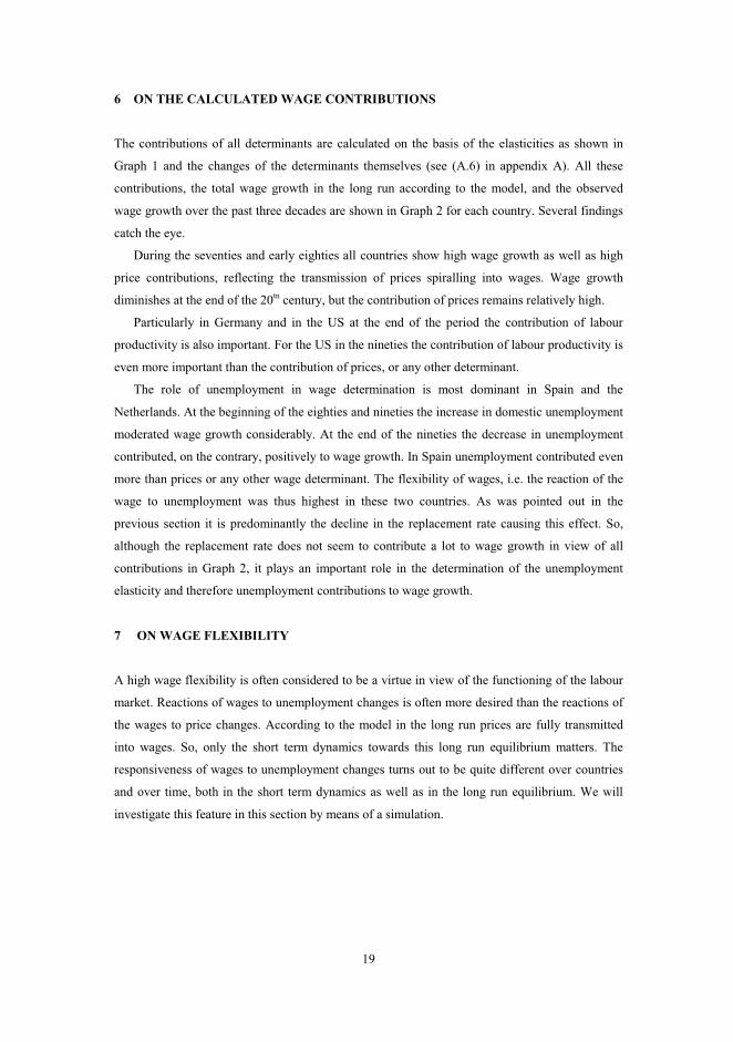
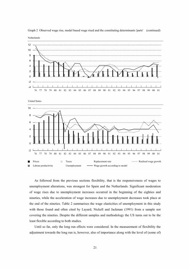
6 ON THE CALCULATED WAGE CONTRIBUTIONS

The contributions of all determinants are calculated on the basis of the elasticities as shown in

Graph 1 and the changes of the determinants themselves (see (A.6) in appendix A). All these

contributions, the total wage growth in the long run according to the model, and the observed

wage growth over the past three decades are shown in Graph 2 for each country. Several findings

catch the eye.

During the seventies and early eighties all countries show high wage growth as well as high

price contributions, reflecting the transmission of prices spiralling into wages. Wage growth

diminishes at the end of the 20tn century, but the contribution of prices remains relatively high.

Particularly in Germany and in the US at the end of the period the contribution of labour

productivity is also important. For the US in the nineties the contribution of labour productivity is

even more important than the contribution of prices, or any other determinant.

The role of unemployment in wage determination is most dominant in Spain and the

Netherlands. At the beginning of the eighties and nineties the increase in domestic unemployment

moderated wage growth considerably. At the end of the nineties the decrease in unemployment

contributed, on the contrary, positively to wage growth. In Spain unemployment contributed even

more than prices or any other wage determinant. The flexibility of wages, i.e. the reaction of the

wage to unemployment was thus highest in these two countries. As was pointed out in the

previous section it is predominantly the decline in the replacement rate causing this effect. So,

although the replacement rate does not seem to contribute a lot to wage growth in view of all

contributions in Graph 2, it plays an important role in the determination of the unemployment

elasticity and therefore unemployment contributions to wage growth.

7 ON WAGE FLEXIBILITY

A high wage flexibility is often considered to be a virtue in view of the functioning of the labour

market. Reactions of wages to unemployment changes is often more desired than the reactions of

the wages to price changes. According to the model in the long run prices are fully transmitted

into wages. So, only the short term dynamics towards this long run equilibrium matters. The

responsiveness of wages to unemployment changes turns out to be quite different over countries

and over time, both in the short term dynamics as well as in the long run equilibrium. We will

investigate this feature in this section by means of a simulation.

20

76 77 78 79 80 81 82 83 84 85 86 87 88 89 90 91 92 93 94 95 96 97 98 99 00 01

-2

0

2

4

6

8

10

Graph 2 Observed wage rise, model based wage rised and the constituting determinants 'parts'

Germany

76 77 78 79 80 81 82 83 84 85 86 87 88 89 90 91 92 93 94 95 96 97 98 99 00 01

-10

-5

0

5

10

15

20

25

Spain

76 77 78 79 80 81 82 83 84 85 86 87 88 89 90 91 92 93 94 95 96 97 98 99 00 01

-4

0

4

8

12

16

Prices

Labour productivity

Taxes

Unemployment

Replacement rate

Wage growth according to model

Realised wage growth

France

21

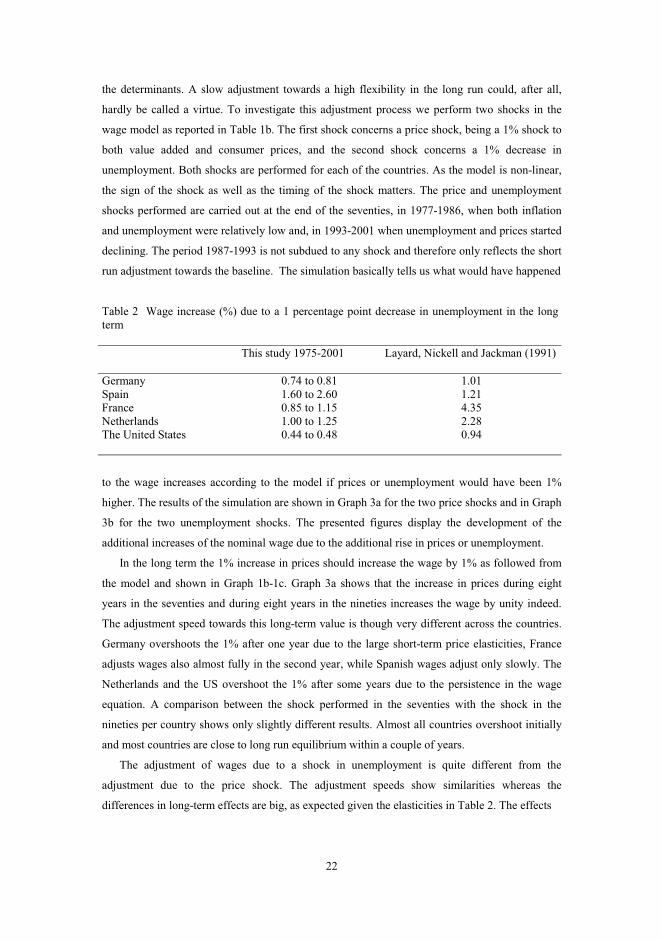
As followed from the previous sections flexibility, that is the responsiveness of wages to

unemployment alterations, was strongest for Spain and the Netherlands. Significant moderation

of wage rises due to unemployment increases occurred in the beginning of the eighties and

nineties, while the acceleration of wage increases due to unemployment decreases took place at

the end of the nineties. Table 2 summarises the wage elasticities of unemployment in this study

with those found and often cited by Layard, Nickell and Jackman (1991) from a sample not

covering the nineties. Despite the different samples and methodology the US turns out to be the

least flexible according to both studies.

Until so far, only the long run effects were considered. In the measurement of flexibility the

adjustment towards the long run is, however, also of importance along with the level of (some of)

76 77 78 79 80 81 82 83 84 85 86 87 88 89 90 91 92 93 94 95 96 97 98 99 00 01

-4

-2

0

2

4

6

8

10

12

Graph 2 Observed wage rise, model based wage rised and the constituting determinants 'parts' (continued)

Netherlands

76 77 78 79 80 81 82 83 84 85 86 87 88 89 90 91 92 93 94 95 96 97 98 99 00 01

-2

0

2

4

6

8

10

Prices

Labour productivity

Taxes

Unemployment

Replacement rate

Wage growth according to model

Realised wage growth

United States

22

the determinants. A slow adjustment towards a high flexibility in the long run could, after all,

hardly be called a virtue. To investigate this adjustment process we perform two shocks in the

wage model as reported in Table 1b. The first shock concerns a price shock, being a 1% shock to

both value added and consumer prices, and the second shock concerns a 1% decrease in

unemployment. Both shocks are performed for each of the countries. As the model is non-linear,

the sign of the shock as well as the timing of the shock matters. The price and unemployment

shocks performed are carried out at the end of the seventies, in 1977-1986, when both inflation

and unemployment were relatively low and, in 1993-2001 when unemployment and prices started

declining. The period 1987-1993 is not subdued to any shock and therefore only reflects the short

run adjustment towards the baseline. The simulation basically tells us what would have happened

Table 2 Wage increase (%) due to a 1 percentage point decrease in unemployment in the long

term

This study 1975-2001 Layard, Nickell and Jackman (1991)

Germany 0.74 to 0.81 1.01

Spain 1.60 to 2.60 1.21

France 0.85 to 1.15 4.35

Netherlands 1.00 to 1.25 2.28

The United States 0.44 to 0.48 0.94

to the wage increases according to the model if prices or unemployment would have been 1%

higher. The results of the simulation are shown in Graph 3a for the two price shocks and in Graph

3b for the two unemployment shocks. The presented figures display the development of the

additional increases of the nominal wage due to the additional rise in prices or unemployment.

In the long term the 1% increase in prices should increase the wage by 1% as followed from

the model and shown in Graph 1b-1c. Graph 3a shows that the increase in prices during eight

years in the seventies and during eight years in the nineties increases the wage by unity indeed.

The adjustment speed towards this long-term value is though very different across the countries.

Germany overshoots the 1% after one year due to the large short-term price elasticities, France

adjusts wages also almost fully in the second year, while Spanish wages adjust only slowly. The

Netherlands and the US overshoot the 1% after some years due to the persistence in the wage

equation. A comparison between the shock performed in the seventies with the shock in the

nineties per country shows only slightly different results. Almost all countries overshoot initially

and most countries are close to long run equilibrium within a couple of years.

The adjustment of wages due to a shock in unemployment is quite different from the

adjustment due to the price shock. The adjustment speeds show similarities whereas the

differences in long-term effects are big, as expected given the elasticities in Table 2. The effects

23

vanish after the first shock period, towards the beginning of the nineties. Wages in the

Netherlands and the US do not return to base immediately, but increase wages for some time due

to persistence. The difference between the two shocking periods per country is moreover stronger

for each country than in case of the price shock. The adjustment speed itself remains the same,

but the long-term elasticities for Germany, Spain and France are lower in absolute terms in the

nineties than in the seventies and the unemployment rate –for instance- is higher. In sum, wage

‘flexibility’ is lower (for Germany 0.76 in 2001 in comparison with 0.79 in 1985, for Spain 1.82

to 1.90, for France 0.83 and 0.92). For the Netherlands and the US the wage increase is slightly

higher (1.21 to 1.18 and 0.53 to 0.52, respectively).

75 77 79 81 83 85 87 89 91 93 95 97 99 01

-0,5

0,0

0,5

1,0

1,5

Ad

dit

ion

al i

ncr

ease

nom

inal

wag

e ra

teGraph 3a Simulation of a price shock

75 77 79 81 83 85 87 89 91 93 95 97 99 01

-0,5

0,0

0,5

1,0

1,5

2,0

2,5

A

ddit

ion

al i

ncr

ease

no

min

al w

age

rate

Germany Spain France Netherlands United States

Graph 3b Simulation of a unemployment shock

24

8 SUMMARY AND CONCLUSIONS

A non-linear wage equation is derived from a theoretical framework describing the wage

bargaining process between employers and employees. The wage rate is determined by labour

productivity, the value added price and the consumer price, the marginal and average tax rates

and further, interrelatedly, the unemployment and replacement rates. This wage equation is

estimated by means of an Error-Correction Model using annual time series of the last three

decades for Germany, Spain, France, the Netherlands and the US. In comparison with the study

of Graafland and Huizinga (1999), who developed this wage bargaining model and estimated the

wage equation for the Netherlands up to 1993, and Peeters and Den Reijer (2001), who applied it

to Ireland, Spain and the Netherlands, main attention is paid here to the end of the nineties when

unemployment sharply dropped. Moreover, wages are no longer assumed to have a unity

elasticity with respect to labour productivity in the long run. However, with the exception of

France and the Netherlands this paramater turned out not to differ significantly from unity. The

importance of dropping this restriction turns out to be important for the estimates and

consequently goodness-of-fit of the model. Three-Stage-Least-Squares is applied to estimate the

model consistently and efficiently in view of the endogeneity of prices in the short-term and

common shocks respectively. So, the ECM is estimated in a system of five equations. In the long

run the non-linear wage relationship with its determinants is imposed and the deep parameters are

identified directly. The estimation results are satisfying, confirming the solidity of the theoretical

wage bargaining framework in combination with the data. The estimated coefficients are used to

compute the (non-constant) elasticities and contributions of the wage determinants to wage

growth. Finally, real and nominal wage flexibilities are assessed for the individual countries.

The main empirical results are the following. Price increases contributed most to wage growth

in the seventies and eighties in all four European countries under investigation and also in the US.

Also the role of labour productivity was important, particularly in Germany and the US. In the US

the contribution of labour productivity to wage growth even dominates at the end of the nineties.

The contributions of taxes and the replacement rate are negligible for all countries. The wage

elasticities of unemployment are highest in Spain and the Netherlands and lowest in the US. At

the end of the nineties the wage elasticity with respect to unemployment increased in absolute

terms and unemployment fell drastically in both Spain and the Netherlands. For these two reasons

the contribution of unemployment to wage growth became more important. For Spain, the

contribution of unemployment was even the dominant factor in the formation of wages in the

nineties. In Spain and the Netherlands a clear turning point in unemployment developments were

probably triggered by favourable labour market policies conducted in the eighties. These policies

led to a reduction of the replacement rate. The replacement rate plays its dominant role in the

unemployment contributions as it is an important determinant in the calculated unemployment

25

elasticities. The higher flexibility of wages for unemployment alterations for Spain and the

Netherlands contrasts to Germany, where the replacement rate did not decrease at the end of the

period, and consequently the unemployment elasticity fell (in absolute terms).

Similar to the labour market study results of Layard, Nickell and Jackman (1991) we also

confirm that the wage formation in the US cannot be called more flexible than in the three largest

European countries or the Netherlands. The flexibility, that is the reaction of wages to

unemployment changes, is by far smaller for the US than for these countries. This feature is

particularly shown in the simulation analysis. Moreover, the short run adjustment in the US of

wages to price changes reveals some stickiness. The low responsiveness of wages to

unemployment in the US might be rationalised by the functioning of its labour market. This

market may adjust towards equilibrium more by quantity adjustments than by wage adjustment.

26

REFERENCES

Auer, P. (2000), Employment revival in Europe: Labour market success in Austria, Denmark,

Ireland and the Netherlands, International Labor Office, Geneva.

Bell, B., S. Nickell and G. Quintini (2000), Wage Equations, Wage Curves and All That, Centre

for Economic Performance, London, September.

Bover, O., P. García-Perea and P. Portugal (2000), Labour market outliers: Lessons from Portugal

and Spain, Economic Policy, pp.381-428.

Bover, O., S. Bentolila and M. Arellano (2001), The distribution of earnings in Spain during the

1980s: the effects of skill, unemployment and union power, CEPR discussion paper, available on

http://www.cepr.org/pubs/dps/dp2770.asp.

Center for Economic Policy Research (1995), Unemployment: Choices for Europe, Monitoring

European Integration 5.

Graafland, J.J. en F.H. Huizinga (1999), Taxes and benefits in a non-linear wage equation, DeEconomist 147, no. 1, pp. 39-54.

Grubb, D., R. Jackman and R. Layard (1983), Wage rigidity and unemployment in OECD

countries, European Economic Review, vol. 21, pp. 11-39.

Grüner, H.P. and C. Hefeker (1999), How will EMU affect inflation and unemployment in

Europe?, Scandinavian Journal of Economics, 101(1), pp. 33-47.

Layard, R., S. Nickell and R. Jackman (1991), Unemployment: Macroeconomic Performance and

the Labour Market, Oxford: Oxford University Press.

Nickell, S. (1997), Unemployment and labor market rigidities: Europe versus North America,

Journal of Economic Perspectives, Volume 11, number 3, pp. 55-74.

Organisation for Economic Co-operation and Development (OECD) (1999), EMU, Facts ,Challenges and Policies , Paris.

Organisation for Economic Co-operation and Development (2002), website

http://oecdpublications.gfi-nb.com.

Peeters, H.M.M. and A.H.J. den Reijer (2001), On wage formation, wage development and

unemployment, De Nederlandsche Bank NV, WO&E no. 677.

27

APPENDIX A DERIVATION OF WAGE EQUATION, WAGE ELASTICITIES AND

CONTRIBUTIONS

In comparison with the wage model used in Graafland and Huizinga (1999) and Peeters and Den

Reijer (2001) the model specified in section 2 takes into account the possibility of diminishing

instead of constant returns of production. Below follows the derivation of the wage equation.

In order to derive the optimal wage the objective function

1( ) ( ( ) )Pq W W T W Wρ α α−Ω ≡ − − − , (1)

where ( )T W is the taxes paid by the employee as a function of W , is differentiated with respect

to W :

1 1( ) ( ( ) ) ( ) (1 )( ( ) ) (1 ) 0T

Pq W W T W W Pq W W T W WW W

ρ α α ρ α αα α− − −∂Ω ∂≡ − − − − + − − − − − = ⇔∂ ∂

( ( ) ) ( )(1 )(1 ) 0T

W T W W Pq WW

ρα α ∂− − − + − − − =

∂

1(1 ) (1 )

1 1m m

tW P q W

t t

ρ αα α α − + − = − + − −

(A1)

where m

Tt

W

∂≡∂

and ( ) (1 )W T W W t− = − .

The wage earned in the official sector

^ ^

(1 ) (1 ) (1 )officialW u R W t u W t= − + − − (4)

and the informal wage

cinformalW P q ργ= (5)

can be substituted into the reservation wage equation

(1 )official informalW W Wβ β= + − (3)

such that the reservation wage equals

28

^

(1 ) (1 (1 )) (1 ) cW W t u R P q ρβ β γ= − − − + − . (A2)

Substitution of (A2) into (A1) and using ^

W W= gives

1(1 ) (1 ) (1 ) (1 (1 )) (1 )

1 1c

m m

tW P q W t u R P q

t t

ρ ραα α α β β γ − + − = − + − − − + − ⇔ − −

1 (1 )1 [1 (1 (1 ))]

1 1 1 1

c

m m

P qtW u R P q

t t

ρρα α β γβ

α α − −+ − − − = + ⇔ − − − −

1 (1 ) (1 )1 [1 (1 (1 ))] 1 1 (1 )

1 1 1 (1 ) (1 ) 1

c

m m

PtW u R P q

t P t

ρα α β γ α β γβα α α β γ α

− − −+ − − − = + − + − − − + − − −

In this last step an arrangement is made to separate the term Pqρ and the constant term, virtues

that follow from the wage equation expressed in logarithms below.

Because, taking logarithmes the wage equation equals

( )( ) ( )

( )( ) ( )

1log log log log 1 1

1 1 1

11log 1 1 1 1 log 1

1 1 1

c

m

m

PW P q

P t

tu R

t

α β γρ

α α β γ

α β γα βα α

−= + + + − − + − −

− − − + − − − + + − − −

(7)

In the econometric analyses mt t= is imposed due to lack of data on the marginal tax rates for all

countries. From this equation the elasticities (see Graph 1) can be calculated. It follows that the

sum of the wage elasticities of value added prices and consumer prices, defined as P∈ and

cP∈ respectively, add to one as it can be derived that

log log1

log logcP Pc

W W

P P

∂ ∂∈ + ∈ ≡ + =∂ ∂

.

The elasticity of wages with respect to productivity, the semi-elasticities of wages with respect to

unemployment and the replacement rate are respectively

log

logq

W

qρ∂∈ ≡ =

∂ (A3)

log (1 )

1 1u

W R

u z

α βα

∂ −∈ ≡ = −∂ − +

(A4)

29

log

1 1R

W u

R z

α βα

∂∈ ≡ = −∂ − +

(A5)

where [1 (1 (1 ))]1

z u Rα β

α≡ − − −

−

The differential equation

, , , , ,

loglog

logci P P q t u R

W id W

i i=

∂ ∂=∂

equals approximately

, , , , ,

log

c

i

i P P q t u R

iW

i=

∆∆ = ∈ (A6)

where logW∆ represents the change of the the gross wage W . In case of semi-elasticities,

multiplication by i∆ instead of the i

i

∆ is taken. The six individual contributions in (A6) and the

wage growth according to the model are provided in Graph 2 for each country in the empirical

analyses.

30

APPENDIX B DATA SOURCES

The time series , , , , ,cW P P q t u come from EUROMON, the multi-country model of De

Nederlandsche Bank. The gross replacement rates are two-year annual series from 'Benefits and

wages', OECD Indicators, from the OECD (2002). These series were interpolated for the purpose

of the analyses here. All series can be received upon request.

Earlier publications in this series as from January 2002

No. 73/2002 The Credit Channel in the Netherlands: Evidence from bank balance sheets

L. de Haan

No. 74/2002 Finance, law and growth during transition: a survey

R.T.A. de Haas

Overview of papers presented at the 4th Annual Conference ‘Understanding Exchange Rates’

held at De Nederlandsche Bank, Amsterdam, 14-16 November 2001 (Nos. 75-82)

No. 75/2002 A Theory of the Currency Denomination of International Trade

P. Bacchetta and E. van Wincoop

No. 76/2002 Commodity Currencies and Empirical Exchange Rate Puzzles

Y. Chen and K. Rogoff

No. 77/2002 Exchange Rate Pass-Through, Exchange Rate Volatility, and Exchange Rate

Disconnect

M.B. Devereux and Ch. Engel

No. 78/2002 Exchange Rates and Fundamentals a Non-Linear Relationship?

P. de Grauwe and I. Vansteenkiste

No. 79/2002 How has the Euro Changed the Foreign Exchange Market?

H. Hau, W. Killeen and M. Moore

No. 80/2002 External Wealth, the Trade Balance, and the Real Exchange Rate

Ph.R. Lane and G.M.Milesi-Ferretti

No. 81/2002 PPP and the Balassa Samuelson Effect: The Role of the Distribution Sector

R. MacDonald and L. Ricci

No. 82/2002 On the Strength of the US Dollar: Can it be Explained by Output Growth?

P.J.G. Vlaar

No. 83/2002 Comovement in International Equity Markets: a Sectoral View

R.P. Berben and W.J. Jansen

No. 84/2002 The Welfare Cost of Structural Distortions and Stochastic Shocks

P.A.D. Cavelaars

No. 85/2002 Double Discretion, International Spillovers and the Welfare Implications of

Monetary Unification

P.A.D. Cavelaars

No. 86/2002 Cyclical Patterns in Profits, Provisioning and Lending of Banks

J.A. Bikker and H. Hu

No. 87/2002 Efficiency and Cost Differences Across Countries in a Unified European

Banking Market

J.A. Bikker

No. 88/2002 Aiming for the Bull’s Eye: Inflation Targeting under Uncertainty

M. Demertzis and N. Viegi

No. 89/2002 The Timing of EU Expansion and the Real Exchange Rate

P.A.D. Cavelaars

No. 90/2002 Spillover of Domestic Regulation to Emerging Markets

A.F. Tieman

No. 91/2002 Foreign Bank Penetration and Private Sector Credit in Central and

Eastern Europe

R.T.A. de Haas and I.P.P. van Lelyveld

No. 92/2002 Does Competition Enhancement Have Permanent Inflation Effects?

P.A.D. Cavelaars

No. 93/2003 Is Financial Market Volatility Informative to Predict Recessions?

N. Valckx, M.J.K de Ceuster and J. Annaert

Overview of papers presented at the 5th Annual Conference ‘Global Linkages and Economic

Performance’ held at De Nederlandsche Bank, Amsterdam, 13 – 15 November 2002

(Nos. 94 – 101)

No. 94/2003 The Trilemma in History: Tradeoffs among Exchange Rates, Monetary Policies,

and Capital Mobility

Maurice Obstfeld, Jay C. Shambaugh and Alan M. Taylor

No. 95/2003 Financial Globalization and Monetary Policy

Helmut Wagner and Wolfram Berger

No. 96/2003 Fancy a stay at the “Hotel California”?

Foreign Direct Investment, Taxation and Exit Costs

Holger Görg

No. 97/2003 Global vs. Local Competition

Patrick Legros and Konrad Stahl

No. 98/2003 Long-Term Global Market Correlations

William N. Goetzmann, Lingfeng Li and K. Geert Rouwenhorst

No. 99/2003 The Importance of Multinational Companies for Global Economic Linkages

W. Jos Jansen and Ad C.J. Stokman

No. 100/2003 Globalisation and Market Structure

J.Peter Neary

No. 101/2003 Is Wealth Increasingly Driving Consumption?

Tamim Bayoumi and Hali Edison

No. 102/2003 On the influence of capital requirements on competition and risk taking in

banking

Peter J.G. Vlaar

No. 103/2003 Robust versus Optimal Rules in Monetary Policy: A note

Maria Demertzis and Alexander F. Tieman

No. 104/2003 The Impact of the Single Market on the Effectiveness of ECB Monetary Policy

Paul Cavelaars

No. 105/2003 Central Bank Transparency in Theory and Practice

Maria Demertzis and Andrew Hughes Hallett

No. 106/2003 The (A)symmetry of shocks in the EMU

Bastiaan A. Verhoef

No. 107/2003 Forecasting inflation: An art as well as a science!

Ard H.J. den Reijer and Peter J.G. Vlaar

No. 108/2003 On Wage Formation, Wage Development and Flexibility:

a comparison between European countries and the United States

Marga Peeters and Ard den Reijer