1

Down but not Out: A Cost of Capital Approach to Fair Value Risk

Margins

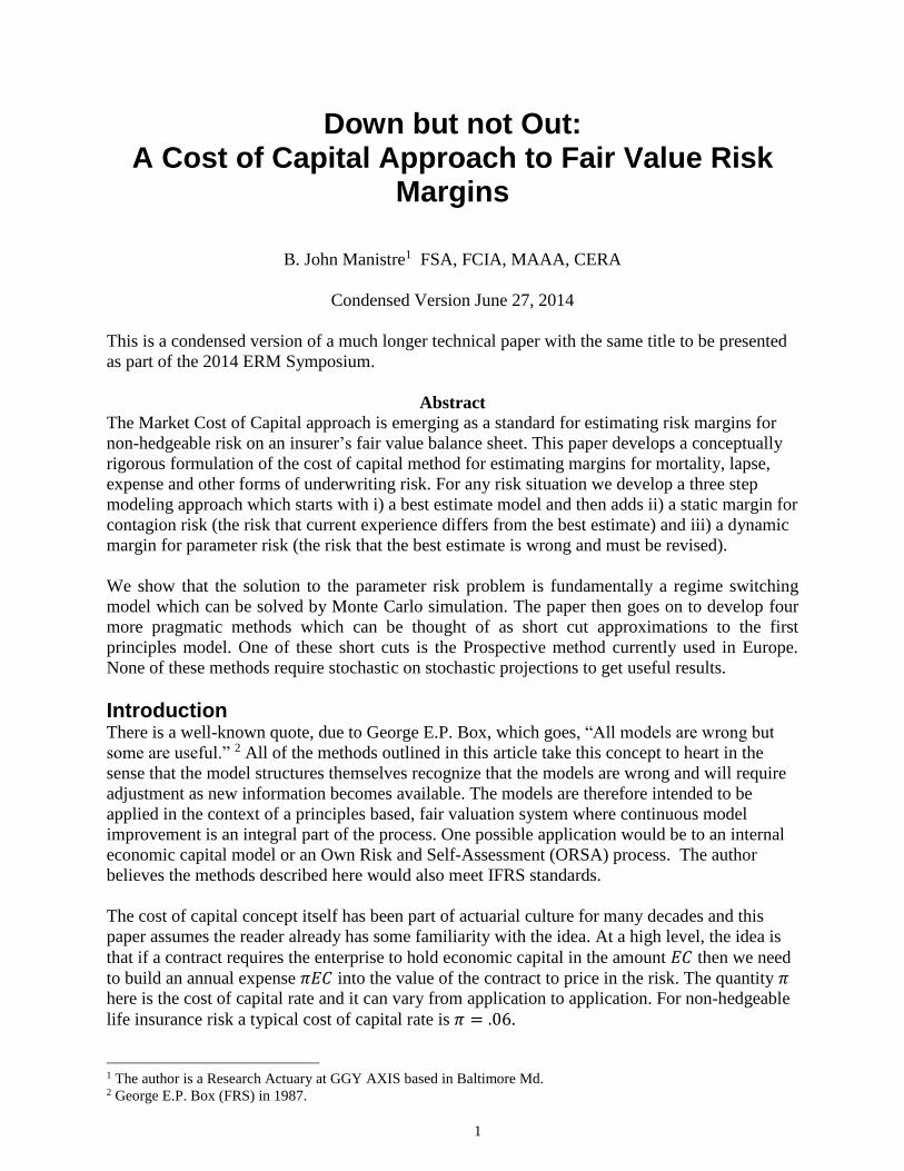
B. John Manistre1 FSA, FCIA, MAAA, CERA

Condensed Version June 27, 2014

This is a condensed version of a much longer technical paper with the same title to be presented

as part of the 2014 ERM Symposium.

Abstract The Market Cost of Capital approach is emerging as a standard for estimating risk margins for

non-hedgeable risk on an insurer’s fair value balance sheet. This paper develops a conceptually

rigorous formulation of the cost of capital method for estimating margins for mortality, lapse,

expense and other forms of underwriting risk. For any risk situation we develop a three step

modeling approach which starts with i) a best estimate model and then adds ii) a static margin for

contagion risk (the risk that current experience differs from the best estimate) and iii) a dynamic

margin for parameter risk (the risk that the best estimate is wrong and must be revised).

We show that the solution to the parameter risk problem is fundamentally a regime switching

model which can be solved by Monte Carlo simulation. The paper then goes on to develop four

more pragmatic methods which can be thought of as short cut approximations to the first

principles model. One of these short cuts is the Prospective method currently used in Europe.

None of these methods require stochastic on stochastic projections to get useful results.

Introduction There is a well-known quote, due to George E.P. Box, which goes, “All models are wrong but

some are useful.” 2 All of the methods outlined in this article take this concept to heart in the

sense that the model structures themselves recognize that the models are wrong and will require

adjustment as new information becomes available. The models are therefore intended to be

applied in the context of a principles based, fair valuation system where continuous model

improvement is an integral part of the process. One possible application would be to an internal

economic capital model or an Own Risk and Self-Assessment (ORSA) process. The author

believes the methods described here would also meet IFRS standards.

The cost of capital concept itself has been part of actuarial culture for many decades and this

paper assumes the reader already has some familiarity with the idea. At a high level, the idea is

that if a contract requires the enterprise to hold economic capital in the amount 𝐸𝐶 then we need

to build an annual expense 𝜋𝐸𝐶 into the value of the contract to price in the risk. The quantity 𝜋

here is the cost of capital rate and it can vary from application to application. For non-hedgeable

life insurance risk a typical cost of capital rate is 𝜋 = .06.

1 The author is a Research Actuary at GGY AXIS based in Baltimore Md. 2 George E.P. Box (FRS) in 1987.

2

There are three themes or common denominators that run through all of the methods discussed

here. These are:

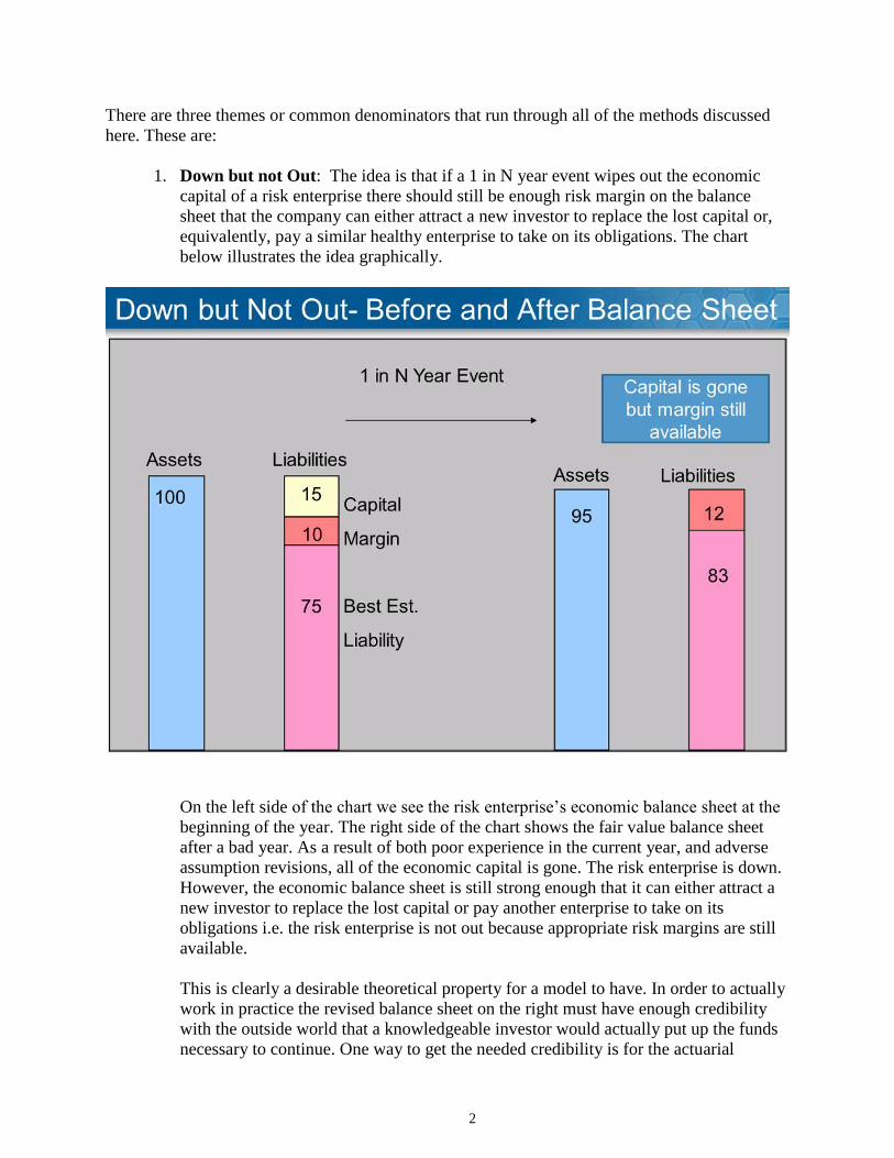
1. Down but not Out: The idea is that if a 1 in N year event wipes out the economic

capital of a risk enterprise there should still be enough risk margin on the balance

sheet that the company can either attract a new investor to replace the lost capital or,

equivalently, pay a similar healthy enterprise to take on its obligations. The chart

below illustrates the idea graphically.

On the left side of the chart we see the risk enterprise’s economic balance sheet at the

beginning of the year. The right side of the chart shows the fair value balance sheet

after a bad year. As a result of both poor experience in the current year, and adverse

assumption revisions, all of the economic capital is gone. The risk enterprise is down.

However, the economic balance sheet is still strong enough that it can either attract a

new investor to replace the lost capital or pay another enterprise to take on its

obligations i.e. the risk enterprise is not out because appropriate risk margins are still

available.

This is clearly a desirable theoretical property for a model to have. In order to actually

work in practice the revised balance sheet on the right must have enough credibility

with the outside world that a knowledgeable investor would actually put up the funds

necessary to continue. One way to get the needed credibility is for the actuarial

3

profession to develop standards of practice that are rigorous enough for the shocked

balance sheet to be credible.

2. Linearity: All of the methods considered here can be formulated as systems of linear

stochastic equations. This has two very general consequences.

a. As is well known, a linear problem usually has a dual version. If you can solve

the primal problem you can also solve the dual to get the same answer. In this

case the primal version of the problem looks like an “actuarial” calculation

where we project capital requirements into the future and then compute

margins as the present value of the cost of capital.

As formulated here, the dual version of the problem looks more like a

“financial engineering” calculation. The process above is reversed by starting

with a concept of risk neutral or risk loaded mortality, lapse etc. and then

determining the corresponding implied economic capital by seeing how the

margins unwind over time.

Put another way, if the present value of margins 𝑀 and the economic capital

𝐸𝐶 are related by an equation of the form

𝑑𝑀

𝑑𝑡= (𝑟 + 𝜇)𝑀 − 𝜋𝐸𝐶,

then the primal version of the method starts by projecting 𝐸𝐶 and then uses the

above relation to calculate margins by discounting. The dual approach

calculates 𝑀 first and then uses a version of the relation above to estimate an

implied economic capital 𝐸𝐶.

b. A second useful consequence of using linear models is that they allow us to

avoid the “stochastic on stochastic” issue that bedevils many other approaches

to the margin issue. Linear models can be calculated scenario by economic

scenario. Any errors we make by ignoring the “stochastic on stochastic” nature

of the problem average out to zero when we sum over a large set of risk neutral

scenarios3.

With this result we can develop the cost of capital ideas in a simple

deterministic economic model, and be confident that the results developed will

continue to apply when we go to a fully stochastic economic model.

Looking at the dual gives us both new theoretical insight and an alternative way to

compute any given model. In particular, the dual approach adds transparency in

the sense that it tells us what the implied “risk neutral” assumptions for mortality,

lapse etc. are.

3 This is a standard result in stochastic calculus which is outlined in the main

technical paper.

4

For any particular application, the primal and dual approaches are equivalent but

can differ in practice for a variety of reasons. One of the paper’s general

conclusions is that solving the primal problem works well for simple applications

but the dual approach can be preferable as the complexity of the application

increases. The main problem with the dual approach is the effort required to

understand why the theory works. The actual implementation is not that difficult.

We take the view that both the primal and dual versions of a model should make

theoretical sense and this leads to a critique of some approaches. For example, the

primal version of the prospective model used in Europe usually looks simple and

reasonable but the dual version may not. This is illustrated in the main paper by

looking at the example of a lapse supported insurance product. It is possible for

the dual problem to exhibit negative risk loaded lapse rates. We offer a

modification to the method, as well as several other approaches, that can resolve

this issue.

3. The basic risk modeling process: This article assumes a three step process for

putting a value on non-hedgeable risk. In a bit more detail, the steps are

a. Develop a best estimate model that is appropriate to the circumstances of the

application. Detailed discussion of this step is outside the scope of this paper

although we do provide a number of examples from life insurance. The key

assumption we make is that our best estimate models are not perfect and are

subject to revision.

b. Hold capital and risk margins for a contagion event i.e. the risk that current

experience may differ substantially from our best estimate.

Imagine, for the sake of clarity, that our best estimate model is a traditional

actuarial mortality table. Even if our table is right on average, we could still

have bad experience in any given year. The classic example of a contagion

event would be a repeat of the 1918 flu epidemic – hence the name contagion

risk.

More recent examples of contagion risk events would be the North American

commercial mortgage meltdown in the early 1990’s4 and the well-known

problems with the US residential mortgage market that led to the financial

crisis of 2008.

A risk enterprise should have sufficient capital and margins that it can

withstand a plausible contagion event and still be able to continue as a going

concern without regulatory intervention. We show that traditional, static, risk

loadings in our parameters can usually deal with this issue.

4 This was caused by the overbuilding of office space during the 1980’s in many North American cities. When the

oversupply became apparent, office rents plummeted. This dragged down property values and triggered defaults on

many of the mortgages used to finance the office towers.

5

c. Hold capital and margins for parameter risk: New information might arrive in

the course of a year that causes the risk enterprise to revise one or more

models. To the extent these model revisions cause the fair value of liabilities to

increase, we need economic capital to absorb the loss. Again we need a margin

model that allows the risk enterprise to withstand the loss and carry on without

regulatory intervention. To deal with this issue, we introduce the concept of a

dynamic loading which arises naturally out of the dual approach.

Static and dynamic loadings differ in the way margin gets released into income over time. If best

estimate assumptions are realized, then any static margin emerges as an experience gain in the

current reporting period. The risk loading is engineered so that the resulting gain is equal to the

cost of holding capital for contagion risk. This is what most actuaries would expect.

By contrast, a dynamic margin is a time dependent loading, which is equal to zero at the

valuation date, and then grades to an ultimate value discussed later. There is very little

experience gain in the current reporting period. The risk margin gets released into income by

pushing out the grading process as time evolves i.e., when we come to do a new valuation, we

establish a new dynamic load which restarts from zero at the new valuation date. If we get the

math right, this process releases the correct amount of margin to pay for the cost of holding

economic capital for parameter risk, while still leaving sufficient margin on the balance sheet for

the future.

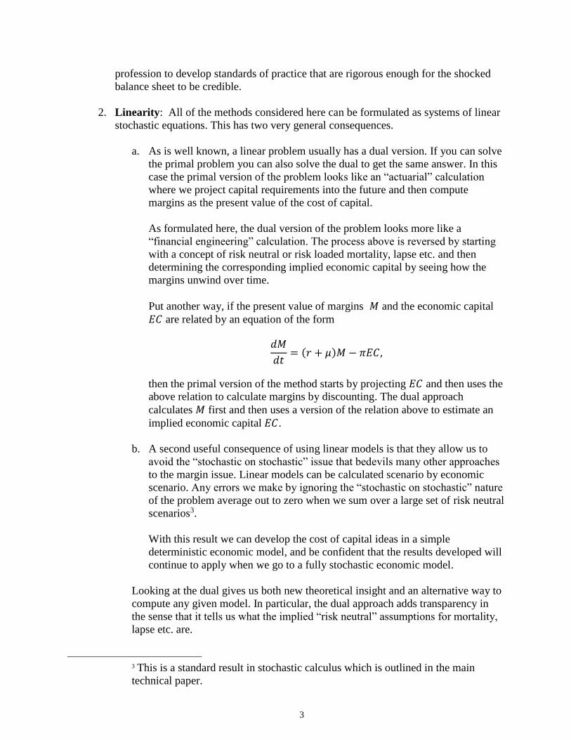
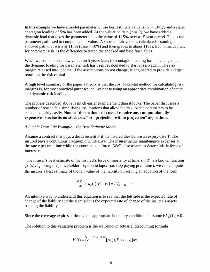
Chart 1 below shows a simple example of the risk loading ideas introduced above.

6

In this example we have a model parameter whose best estimate value is 𝜃0 = 100% and a static

contagion loading of 5% has been added. At the valuation date (𝑡 = 0), we have added a

dynamic load that takes the parameter up to the value of 115% over a 15 year period. This is the

parameter path used to compute a fair value. A shocked fair value is calculated assuming a

shocked path that starts at 115% (base + 10%) and then grades to about 119%. Economic capital,

for parameter risk, is the difference between the shocked and base fair values.

When we come to do a new valuation 5 years later, the contagion loading has not changed but

the dynamic loading for parameter risk has been recalculated to start at zero again. The risk

margin released into income, if the assumptions do not change, is engineered to provide a target

return on the risk capital.

A high level summary of the paper’s theory is that the cost of capital method for calculating risk

margins is, for most practical purposes, equivalent to using an appropriate combination of static

and dynamic risk loadings.

The process described above is much easier to implement than it looks. The paper discusses a

number of reasonable simplifying assumptions that allow the risk loaded parameters to be

calculated fairly easily. None of the methods discussed require any computationally

expensive “stochastic on stochastic” or “projection within projection” algorithms.

A Simple Term Life Example – the Best Estimate Model

Assume a contract that pays a death benefit F if the insured dies before an expiry date T. The

insured pays a continuous premium g while alive. The insurer incurs maintenance expenses at

the rate e per unit time while the contract is in force. We’ll also assume a deterministic force of

interest 𝑟.

The insurer’s best estimate of the insured’s force of mortality at time Ts is a known function

)(0 s . Ignoring the policyholder’s option to lapse (i.e. stop paying premiums), we can compute

the insurer’s best estimate of the fair value of the liability by solving an equation of the form

.])[( 0000 egrVVFt

dt

dV

An intuitive way to understand this equation is to say that the left side is the expected rate of

change of the liability and the right side is the expected rate of change of the insurer’s assets

backing the liability.

Since the coverage expires at time T the appropriate boundary condition to assume is 0)(0 TV .

The solution to this valuation problem is the well-known actuarial discounting formula

.])([)( 0

]))((

0

0

dsgeFsetV

T

t

dvvrs

t

7

The best estimate value 0V is the actuarial present value of death benefits and expenses offset by

the present value of gross premiums.

A Simple Term Life Example - Contagion Risk and Static Margins

Now assume that the insurer holds capital to protect its solvency in the event of a contagion loss

such as a repeat of the 1918 flu epidemic. The insurer has determined that such an event would

result in )(tQ additional deaths per life exposed. If V is the value of the contract, which

includes margin for this risk, then the amount of capital the insurer must hold is ][ VFQ since

this is the economic loss that would occur if additional Q deaths were to occur at time t.

Letting denote the insurer’s cost of capital rate (e.g. 6.00%), the new valuation equation

should include the cost of contagion risk capital as an additional expense i.e.

].[])[(0 VFQegrVVFtdt

dV

But this can easily be rewritten as

.]][)([ 0 egrVVFQtdt

dV

This shows that including margin for the cost of holding contagion risk capital is equivalent to

simply adding a load Q to the best estimate force of mortality 0 . We will refer to this process

as one of adding a static margin or a contagion loading.

The result illustrated is simple, easy to implement, and makes sense as long as 0][ VFQ .

For this example it is not hard to show what VF as long as the premiums and expenses are

reasonable relative to the death benefit. Under this assumption, the contagion shock Q should

be a positive number and set at a level consistent with the insurer’s overall capital target (e.g. one

year VaR at the 99.5% level).

It is worth discussing why this model satisfies the “down but not out” principle. Assuming

mortality contagion is our only risk issue, an investor is asked to put up economic capital in the

amount )]()[()( tVFtQtEC . The insurer then charges the customer a premium sufficient to

cover the cost of expenses and death claims at the contagion loaded level.

To the extent best estimate assumptions are realized, the insurer will recognize economic profits

equal to the margin release plus interest on the economic capital. The total economic return to

the investor is then ][)( VFQr .

At the end of the period, the insurer returns the original capital, and profits, to the shareholder

and then asks for a new capital infusion in the amount ∆𝑄(𝑡 + 1)[𝐹 − 𝑉(𝑡 + 1)] to finance the

risk taking in the next period. We assume the investor is willing to do this because the product

has been engineered to provide the same expected return on this new, higher or lower, capital

amount in the following time period.

8

If experience is better than expected, the return in the current period will be higher than (𝑟 + 𝜋)

and, if worse, the return will be lower and possibly negative. We can imagine the following

conversation between an investor and company management.

Management: Hello Mr. Investor, welcome to the insurance business. I have some good news

and some bad news.

Investor: I’m not sure I like the sound of that.

Management: The bad news is that we have had some adverse mortality experience this year and

most of our available risk capital is gone. The good news is that there are still sufficient loadings

in the future mortality rates that you can expect a reasonable return on your investment, if you

replace the lost capital now.

Investor: How can I be confident this won’t happen again?

Management: You can’t. This is a risk business. The company’s actuaries have followed all

appropriate professional standards of practice in choosing methods, assumptions and

performing the actual calculations. It is possible that we could have another bad year before the

business has run off. If you are uncomfortable with that, you are investing in the wrong

business.

To the extent management’s models and assumptions have credibility with the appropriate

investor public, the company can withstand a loss up to the contagion capital level and still be

strong enough to recapitalize and carry-on. There would be no need for regulatory intervention.

This is what “down but not out” means in this paper.

Finally the investor asks, “What happens if you discover one or more of your assumptions is

wrong and must be revised?” In order to answer this question we have to extend the model to

cover parameter risk.

A Simple Term Life Example -Parameter Risk and Dynamic Margins

The previous section argued that the first two steps of our risk modeling process resulted in a

contagion loaded force of mortality equal to 𝜇(𝑡) = 𝜇0(𝑡) + 𝜋∆𝑄(𝑡). This would be the force of

mortality used in a traditional actuarial valuation in order to provide a margin for contagion risk.

We now consider the risk that either the best estimate force of mortality assumption )(0 t or the

contagion shock ∆𝑄 could be wrong. New information might arrive which leads the insurer to set

a new contagion loaded assumption . Letting V denote the relevant shocked fair value, we

need to hold risk capital in the amount .ˆ VV

The size of the shock ∆𝜇 should reflect a plausible assumption change over the course of one

year at something like the 99.5% VaR level. The size of the shock would then reflect the

inherent riskiness or “liquidity” of the business. Shocks for blocks of traditional business that are

well understood would presumably be smaller than shocks for newer or less liquid types of

9

business. Ideally, there should be some industry consensus around the principles used to choose

the shock.

The fundamental valuation equation, which incorporates both contagion risk and parameter risk,

now becomes

],ˆ[][])[(0 VVVFQegrVVFtdt

dV

or

].ˆ[])[( VVegrVVFtdt

dV

This seems simple enough until we consider how we should calculate V . This is a reserve, based

on a mortality assumption which could again turn out to be wrong. The value V also

needs to include a margin for parameter risk, the risk that the mortality assumption might need to

change again. Letting )2(V denote a double shocked fair value, we would need to hold parameter

risk capital in the amount VV ˆˆ )2( in a shocked world.

The obvious extension of the equation above is then to write

]ˆˆ[ˆ]ˆ)][()([ˆ

)2( VVegVrVFttdt

Vd .

This equation makes the reasonable assumption that the shocked contagion loaded force of

mortality used to calculate V is . The problem is that “down but not out” means we have

had to introduce a second shocked reserve value )2(V which, presumably, depends on a second

level of parameter shock )2( and a third contagion-loaded force of mortality )2( .

We seem to be trapped in an impractical infinite regress. The reserve V depends on V which

depends on )2(V , and so on. This is known as the circularity problem.

A large part of the paper is devoted to solving the circularity problem. The paper does enough

theoretical analysis to come up with a true first principles approach to calculating the model and

then develops four very practical short cut methods. There is a wide range of practical problems

where all four short cuts produce very similar results.

It turns out that it is useful to think of the short cut methods as pragmatic approximations to a

model where we have a geometric hierarchy of assumption levels ,...,, )2(

where 1)( nn for some constant 10 . The 𝑛′𝑡ℎ level in the shock hierarchy

would then be given by

1,

1,1

1... 1)(

n

n

nn

10

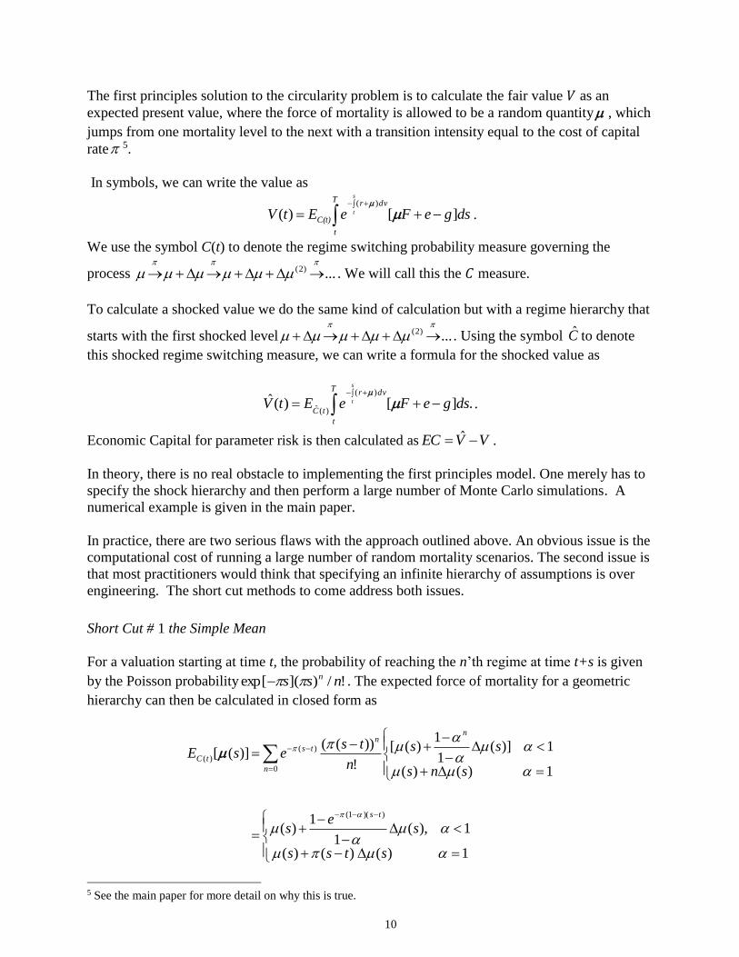
The first principles solution to the circularity problem is to calculate the fair value 𝑉 as an

expected present value, where the force of mortality is allowed to be a random quantity , which

jumps from one mortality level to the next with a transition intensity equal to the cost of capital

rate 5.

In symbols, we can write the value as

dsgeFeEtV

T

t

dvr

C(t)

s

t ][)()(

.

We use the symbol C(t) to denote the regime switching probability measure governing the

process ...)2(

. We will call this the 𝐶 measure.

To calculate a shocked value we do the same kind of calculation but with a regime hierarchy that

starts with the first shocked level ...)2(

. Using the symbol C to denote

this shocked regime switching measure, we can write a formula for the shocked value as

.][)(ˆ)(

)(ˆ dsgeFeEtV

T

t

dvr

tC

s

t

.

Economic Capital for parameter risk is then calculated as VVEC ˆ .

In theory, there is no real obstacle to implementing the first principles model. One merely has to

specify the shock hierarchy and then perform a large number of Monte Carlo simulations. A

numerical example is given in the main paper.

In practice, there are two serious flaws with the approach outlined above. An obvious issue is the

computational cost of running a large number of random mortality scenarios. The second issue is

that most practitioners would think that specifying an infinite hierarchy of assumptions is over

engineering. The short cut methods to come address both issues.

Short Cut # 1 the Simple Mean

For a valuation starting at time t, the probability of reaching the n’th regime at time t+s is given

by the Poisson probability !/)](exp[ nss n . The expected force of mortality for a geometric

hierarchy can then be calculated in closed form as

1)()()(

1),(1

1)(

1)()(

1)](1

1)([

!

))(()]([

))(1(

0

)(

)(

stss

se

s

sns

ss

n

tsesE

ts

n

nn

ts

tC

5 See the main paper for more detail on why this is true.

11

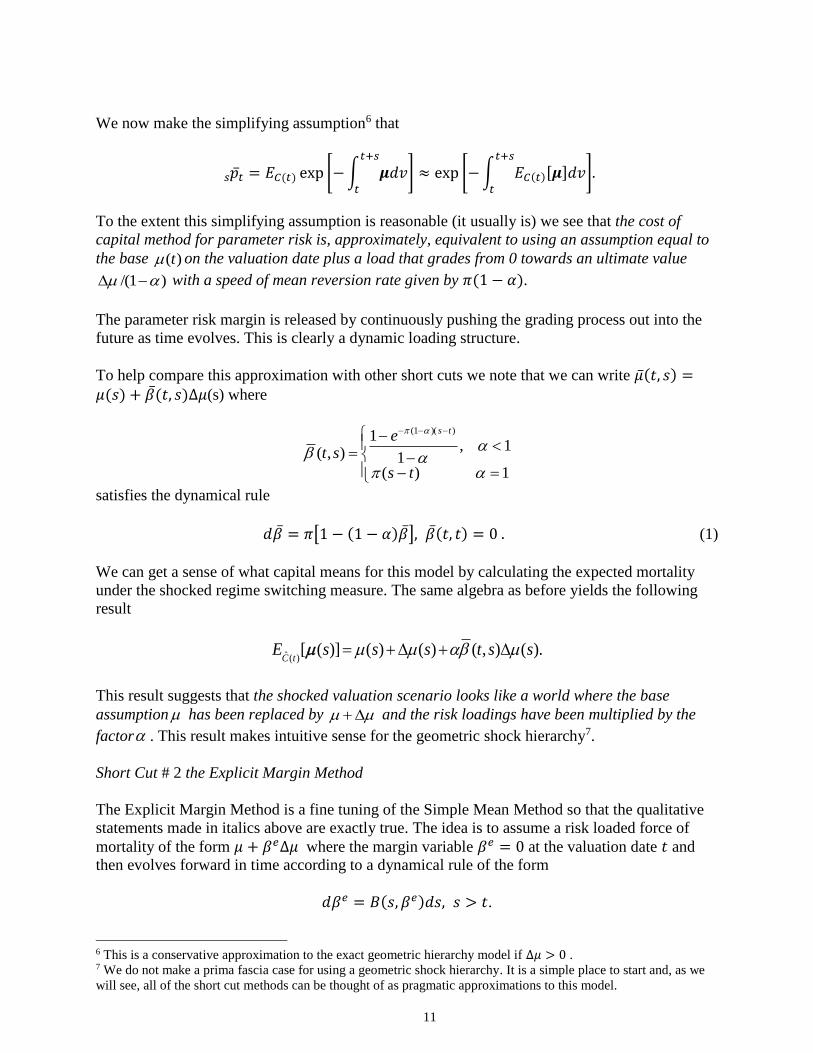
We now make the simplifying assumption6 that

��𝑡𝑠 = 𝐸𝐶(𝑡) exp [− ∫ 𝝁𝑑𝑣𝑡+𝑠

𝑡

] ≈ exp [− ∫ 𝐸𝐶(𝑡)[𝝁]𝑑𝑣𝑡+𝑠

𝑡

].

To the extent this simplifying assumption is reasonable (it usually is) we see that the cost of

capital method for parameter risk is, approximately, equivalent to using an assumption equal to

the base )(t on the valuation date plus a load that grades from 0 towards an ultimate value

)1/( with a speed of mean reversion rate given by 𝜋(1 − 𝛼).

The parameter risk margin is released by continuously pushing the grading process out into the

future as time evolves. This is clearly a dynamic loading structure.

To help compare this approximation with other short cuts we note that we can write ��(𝑡, 𝑠) =𝜇(𝑠) + ��(𝑡, 𝑠)∆𝜇(s) where

1)(

1,1

1),(

))(1(

ts

est

ts

satisfies the dynamical rule

𝑑�� = 𝜋[1 − (1 − 𝛼)��], ��(𝑡, 𝑡) = 0 . (1)

We can get a sense of what capital means for this model by calculating the expected mortality

under the shocked regime switching measure. The same algebra as before yields the following

result

).(),()()()]([)(ˆ sstsssE

tC

This result suggests that the shocked valuation scenario looks like a world where the base

assumption has been replaced by and the risk loadings have been multiplied by the

factor . This result makes intuitive sense for the geometric shock hierarchy7.

Short Cut # 2 the Explicit Margin Method

The Explicit Margin Method is a fine tuning of the Simple Mean Method so that the qualitative

statements made in italics above are exactly true. The idea is to assume a risk loaded force of

mortality of the form 𝜇 + 𝛽𝑒∆𝜇 where the margin variable 𝛽𝑒 = 0 at the valuation date 𝑡 and

then evolves forward in time according to a dynamical rule of the form

𝑑𝛽𝑒 = 𝐵(𝑠, 𝛽𝑒)𝑑𝑠, 𝑠 > 𝑡.

6 This is a conservative approximation to the exact geometric hierarchy model if ∆𝜇 > 0 . 7 We do not make a prima fascia case for using a geometric shock hierarchy. It is a simple place to start and, as we

will see, all of the short cut methods can be thought of as pragmatic approximations to this model.

12

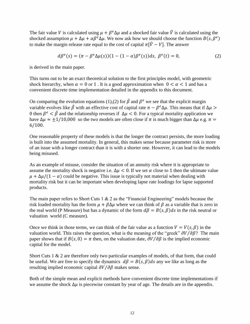
The fair value 𝑉 is calculated using 𝜇 + 𝛽𝑒∆𝜇 and a shocked fair value �� is calculated using the

shocked assumption 𝜇 + ∆𝜇 + 𝛼𝛽𝑒∆𝜇. We now ask how we should choose the function 𝐵(𝑠, 𝛽𝑒)

to make the margin release rate equal to the cost of capital 𝜋[�� − 𝑉]. The answer

𝑑𝛽𝑒(𝑠) = (𝜋 − 𝛽𝑒∆𝜇(𝑠))(1 − (1 − 𝛼)𝛽𝑒(𝑠))𝑑𝑠, 𝛽𝑒(𝑡) = 0, (2)

is derived in the main paper.

This turns out to be an exact theoretical solution to the first principles model, with geometric

shock hierarchy, when 𝛼 = 0 or 1 . It is a good approximation when 0 < 𝛼 < 1 and has a

convenient discrete time implementation detailed in the appendix to this document.

On comparing the evolution equations (1),(2) for �� and 𝛽𝑒 we see that the explicit margin

variable evolves like �� with an effective cost of capital rate 𝜋 − 𝛽𝑒∆𝜇. This means that if ∆𝜇 >0 then 𝛽𝑒 < �� and the relationship reverses if ∆𝜇 < 0. For a typical mortality application we

have ∆𝜇 ≈ ±1/10,000 so the two models are often close if 𝜋 is much bigger than ∆𝜇 e.g. 𝜋 =6/100.

One reasonable property of these models is that the longer the contract persists, the more loading

is built into the assumed mortality. In general, this makes sense because parameter risk is more

of an issue with a longer contract than it is with a shorter one. However, it can lead to the models

being misused.

As an example of misuse, consider the situation of an annuity risk where it is appropriate to

assume the mortality shock is negative i.e. ∆𝜇 < 0. If we set 𝛼 close to 1 then the ultimate value

𝜇 + ∆𝜇/(1 − 𝛼) could be negative. This issue is typically not material when dealing with

mortality risk but it can be important when developing lapse rate loadings for lapse supported

products.

The main paper refers to Short Cuts 1 & 2 as the “Financial Engineering” models because the

risk loaded mortality has the form 𝜇 + 𝛽∆𝜇 where we can think of 𝛽 as a variable that is zero in

the real world (P Measure) but has a dynamic of the form 𝑑𝛽 = 𝐵(𝑠, 𝛽)𝑑𝑠 in the risk neutral or

valuation world (C measure).

Once we think in those terms, we can think of the fair value as a function 𝑉 = 𝑉(𝑠, 𝛽) in the

valuation world. This raises the question, what is the meaning of the “greek” 𝜕𝑉 𝜕𝛽⁄ ? The main

paper shows that if 𝐵(𝑠, 0) = 𝜋 then, on the valuation date, 𝜕𝑉 𝜕𝛽⁄ is the implied economic

capital for the model.

Short Cuts 1 & 2 are therefore only two particular examples of models, of that form, that could

be useful. We are free to specify the dynamics 𝑑𝛽 = 𝐵(𝑠, 𝛽)𝑑𝑠 any we like as long as the

resulting implied economic capital 𝜕𝑉 𝜕𝛽⁄ makes sense.

Both of the simple mean and explicit methods have convenient discrete time implementations if

we assume the shock ∆𝜇 is piecewise constant by year of age. The details are in the appendix.

13

Two Actuarial Short Cuts (3 & 4)

The previous models started with a version of the first principles model and then made a

simplifying assumption which allowed us to analyze the continuous time version of the model.

For Short Cuts 3 & 4 we make a more “actuarial” simplifying assumption which, somewhat

surprisingly, ends up taking us to almost the same place as before.

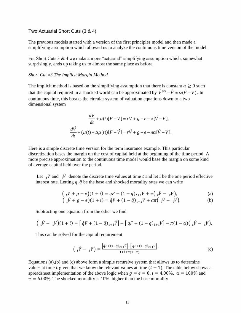
Short Cut #3 The Implicit Margin Method

The implicit method is based on the simplifying assumption that there is constant 𝛼 ≥ 0 such

that the capital required in a shocked world can be approximated by )ˆ(ˆˆ )2( VVVV . In

continuous time, this breaks the circular system of valuation equations down to a two

dimensional system

].ˆ[ˆ]ˆ))[()((ˆ

],ˆ[])[(

VVegVrVFttdt

Vd

VVegrVVFtdt

dV

Here is a simple discrete time version for the term insurance example. This particular

discretization bases the margin on the cost of capital held at the beginning of the time period. A

more precise approximation to the continuous time model would base the margin on some kind

of average capital held over the period.

Let 𝑉𝑡 and ��𝑡 denote the discrete time values at time 𝑡 and let 𝑖 be the one period effective

interest rate. Letting 𝑞, �� be the base and shocked mortality rates we can write

( 𝑉𝑡 + 𝑔 − 𝑒)(1 + 𝑖) = 𝑞𝐹 + (1 − 𝑞) 𝑉𝑡+1 + 𝜋( ��𝑡 − 𝑉𝑡 ), (a)

( ��𝑡 + 𝑔 − 𝑒)(1 + 𝑖) = ��𝐹 + (1 − ��) ��𝑡+1 + 𝛼𝜋( ��𝑡 − 𝑉𝑡 ). (b)

Subtracting one equation from the other we find

( ��𝑡 − 𝑉𝑡 )(1 + 𝑖) = [ ��𝐹 + (1 − ��) ��𝑡+1 ] − [ 𝑞𝐹 + (1 − 𝑞) 𝑉𝑡+1 ] − 𝜋(1 − 𝛼)( ��𝑡 − 𝑉𝑡 ).

This can be solved for the capital requirement

( ��𝑡 − 𝑉𝑡 ) =[��𝐹+(1−��) 𝑉𝑡+1 ]−[ 𝑞𝐹+(1−𝑞) 𝑉𝑡+1 ]

1+𝑖+𝜋(1−𝛼) (c)

Equations (a),(b) and (c) above form a simple recursive system that allows us to determine

values at time 𝑡 given that we know the relevant values at time (𝑡 + 1). The table below shows a

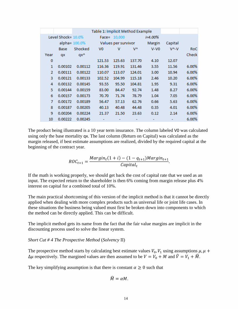
spreadsheet implementation of the above logic when 𝑔 = 𝑒 = 0, 𝑖 = 4.00%, 𝛼 = 100% and

𝜋 = 6.00%. The shocked mortality is 10% higher than the base mortality.

14

The product being illustrated is a 10 year term insurance. The column labeled V0 was calculated

using only the base mortality qx. The last column (Return on Capital) was calculated as the

margin released, if best estimate assumptions are realized, divided by the required capital at the

beginning of the contract year.

𝑅𝑂𝐶𝑡+1 =𝑀𝑎𝑟𝑔𝑖𝑛𝑡(1 + 𝑖) − (1 − 𝑞𝑡+1)𝑀𝑎𝑟𝑔𝑖𝑛𝑡+1

𝐶𝑎𝑝𝑖𝑡𝑎𝑙𝑡.

If the math is working properly, we should get back the cost of capital rate that we used as an

input. The expected return to the shareholder is then 6% coming from margin release plus 4%

interest on capital for a combined total of 10%.

The main practical shortcoming of this version of the implicit method is that it cannot be directly

applied when dealing with more complex products such as universal life or joint life cases. In

these situations the business being valued must first be broken down into components to which

the method can be directly applied. This can be difficult.

The implicit method gets its name from the fact that the fair value margins are implicit in the

discounting process used to solve the linear system.

Short Cut # 4 The Prospective Method (Solvency II)

The prospective method starts by calculating best estimate values 𝑉0, 𝑉1 using assumptions 𝜇, 𝜇 +∆𝜇 respectively. The margined values are then assumed to be 𝑉 = 𝑉0 + 𝑀 and �� = 𝑉1 + ��.

The key simplifying assumption is that there is constant 𝛼 ≥ 0 such that

�� = 𝛼𝑀.

15

This is clearly similar in spirit to the assumption )ˆ(ˆˆ )2( VVVV underlying the implicit

method. It is another way to get around the circularity issue.

Having made this assumption, the economic capital is given by �� − 𝑉 = 𝑉1 − 𝑉0 − (1 − 𝛼)𝑀.

The present value of margins is then calculated by discounting the cost of capital using interest

and base mortality i.e.

𝑑𝑀

𝑑𝑡= (𝑟 + 𝜇)𝑀 − 𝜋[𝑉1 − 𝑉0 − (1 − 𝛼)𝑀].

This implies that

𝑀(𝑡) = ∫ 𝑒− ∫ (𝑟+𝜇+𝜋(1−𝛼))𝑑𝑣]𝑠

𝑡

∞

𝑡

𝜋[𝑉1(𝑠) − 𝑉0(𝑠)]𝑑𝑠.

The prospective method was adopted by European regulators in 2010 for the Solvency II

Quantitative Impact Study #5. Their specification set 𝛼 = 1 for all products and they also

allowed an illiquidity premium 𝜗 to be added to the risk free rate when calculating 𝑉0, 𝑉1, but not

𝑀.

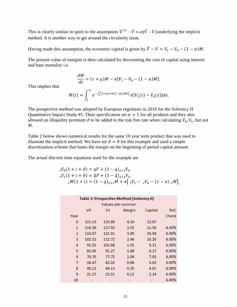
Table 2 below shows numerical results for the same 10 year term product that was used to

illustrate the implicit method. We have set 𝜗 = 0 for this example and used a simple

discretization scheme that bases the margin on the beginning of period capital amount.

The actual discrete time equations used for the example are

𝑉𝑡 0(1 + 𝑖 + 𝜗) = 𝑞𝐹 + (1 − 𝑞) 𝑉𝑡+1 0,

𝑉𝑡 1(1 + 𝑖 + 𝜗) = ��𝐹 + (1 − ��) 𝑉𝑡+1 1,

𝑀𝑡 (1 + 𝑖) = (1 − 𝑞) 𝑀𝑡+1 + 𝜋[ 𝑉𝑡 1 − 𝑉𝑡 0 − (1 − 𝛼) 𝑀𝑡 ].

16

The actual values for margins and capital are not identical to the implicit method but they are

close enough that they are equal at the displayed level of precision. If we went out further in time

we would eventually see a difference.

The main paper shows that the continuous time version of both actuarial short cuts can be

formulated as financial engineering methods, if we choose to do so.

Comparing the Short Cuts – Duality

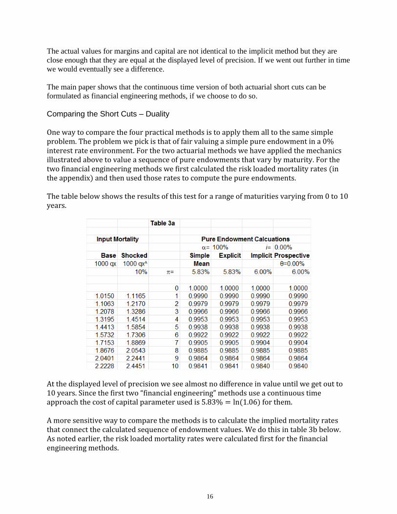
One way to compare the four practical methods is to apply them all to the same simple problem. The problem we pick is that of fair valuing a simple pure endowment in a 0% interest rate environment. For the two actuarial methods we have applied the mechanics illustrated above to value a sequence of pure endowments that vary by maturity. For the two financial engineering methods we first calculated the risk loaded mortality rates (in the appendix) and then used those rates to compute the pure endowments. The table below shows the results of this test for a range of maturities varying from 0 to 10 years.

At the displayed level of precision we see almost no difference in value until we get out to 10 years. Since the first two “financial engineering” methods use a continuous time approach the cost of capital parameter used is 5.83% = ln(1.06) for them. A more sensitive way to compare the methods is to calculate the implied mortality rates that connect the calculated sequence of endowment values. We do this in table 3b below. As noted earlier, the risk loaded mortality rates were calculated first for the financial engineering methods.

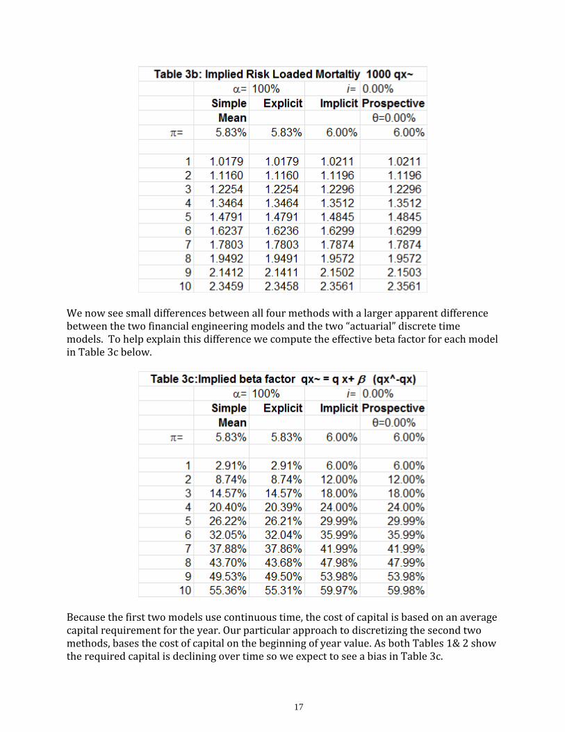
17

We now see small differences between all four methods with a larger apparent difference between the two financial engineering models and the two “actuarial” discrete time models. To help explain this difference we compute the effective beta factor for each model in Table 3c below.

Because the first two models use continuous time, the cost of capital is based on an average capital requirement for the year. Our particular approach to discretizing the second two methods, bases the cost of capital on the beginning of year value. As both Tables 1& 2 show the required capital is declining over time so we expect to see a bias in Table 3c.

18

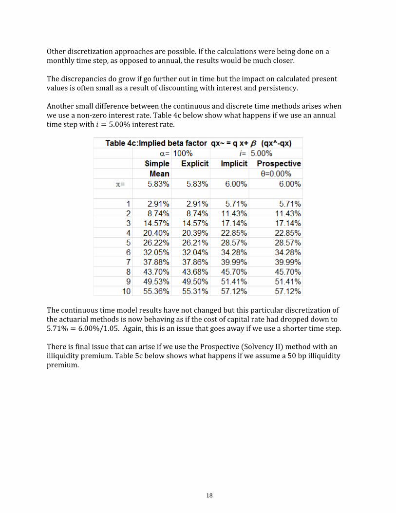
Other discretization approaches are possible. If the calculations were being done on a monthly time step, as opposed to annual, the results would be much closer. The discrepancies do grow if go further out in time but the impact on calculated present values is often small as a result of discounting with interest and persistency. Another small difference between the continuous and discrete time methods arises when we use a non-zero interest rate. Table 4c below show what happens if we use an annual time step with 𝑖 = 5.00% interest rate.

The continuous time model results have not changed but this particular discretization of the actuarial methods is now behaving as if the cost of capital rate had dropped down to 5.71% = 6.00%/1.05. Again, this is an issue that goes away if we use a shorter time step. There is final issue that can arise if we use the Prospective (Solvency II) method with an illiquidity premium. Table 5c below shows what happens if we assume a 50 bp illiquidity premium.

19

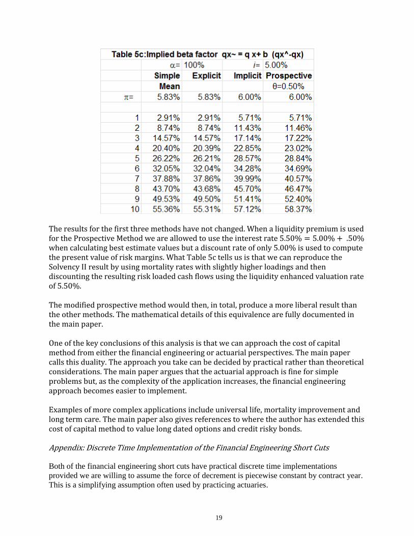
The results for the first three methods have not changed. When a liquidity premium is used for the Prospective Method we are allowed to use the interest rate 5.50% = 5.00% + .50% when calculating best estimate values but a discount rate of only 5.00% is used to compute the present value of risk margins. What Table 5c tells us is that we can reproduce the Solvency II result by using mortality rates with slightly higher loadings and then discounting the resulting risk loaded cash flows using the liquidity enhanced valuation rate of 5.50%. The modified prospective method would then, in total, produce a more liberal result than the other methods. The mathematical details of this equivalence are fully documented in the main paper. One of the key conclusions of this analysis is that we can approach the cost of capital method from either the financial engineering or actuarial perspectives. The main paper calls this duality. The approach you take can be decided by practical rather than theoretical considerations. The main paper argues that the actuarial approach is fine for simple problems but, as the complexity of the application increases, the financial engineering approach becomes easier to implement. Examples of more complex applications include universal life, mortality improvement and long term care. The main paper also gives references to where the author has extended this cost of capital method to value long dated options and credit risky bonds.

Appendix: Discrete Time Implementation of the Financial Engineering Short Cuts

Both of the financial engineering short cuts have practical discrete time implementations

provided we are willing to assume the force of decrement is piecewise constant by contract year.

This is a simplifying assumption often used by practicing actuaries.

20

Suppose the issue age of our life is 𝑥 and we measure time from the issue date. On the valuation

date the life is aged 𝑥 + 𝑡 and our best estimate mortality rate plus contagion load is 𝑞[𝑥]+𝑠 and

the parameter shocked value is ��[𝑥]+𝑠 for 𝑠 ≥ 𝑡. We are using standard select and ultimate

notation. The goal is to come up with a practical way to calculate risk loaded mortality rates

𝑞{[𝑥]+𝑡}+𝑠 for 𝑠 ≥ 0 that reflect the impact of adding an appropriate dynamic margin for

parameter risk after the valuation date. This is a doubly select and ultimate structure since the

risk margin process begins on the valuation date.

Define the decrement shock ∆𝜇𝑠 by

1 − ��[𝑥]+𝑡+𝑠 = (1 − 𝑞[𝑥]+𝑡+𝑠)𝑒−∆𝜇𝑠 , 𝑠 = 0,1,2, …

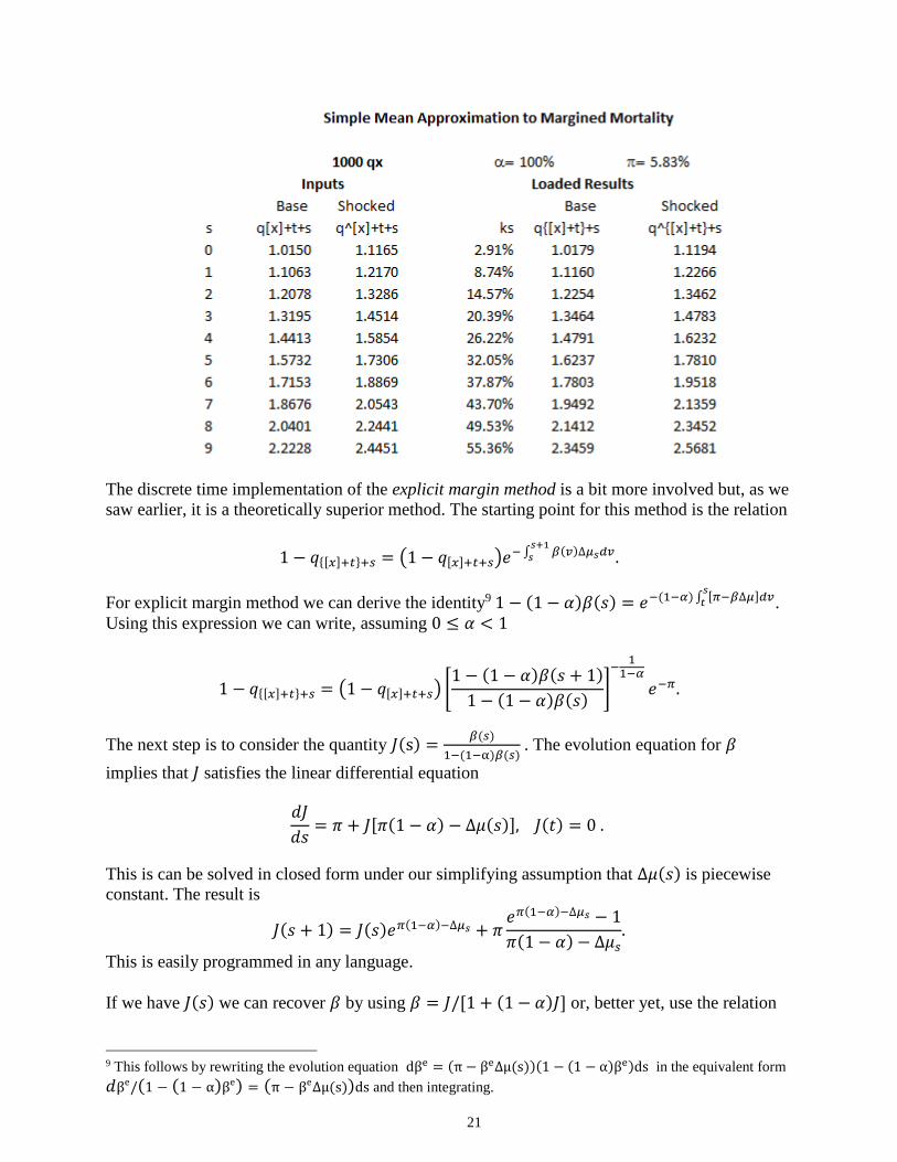
For the simple mean approximation, we can go from one loaded persistency factor ��[𝑥]+𝑡𝑠 to the

next by

��[𝑥]+𝑡𝑠+1 = ��[𝑥]+𝑡𝑒− ∫ (𝜇(𝑣)+��(𝑣)∆𝜇𝑠)𝑑𝑣𝑠+1

𝑠𝑠

= ��[𝑥]+𝑡(1 − 𝑞[𝑥]+𝑡+𝑠)𝑒− ∫ ��(𝑣)∆𝜇𝑠𝑑𝑣𝑠+1

𝑠𝑠 ,

= ��[𝑥]+𝑡(1 − 𝑞[𝑥]+𝑡+𝑠)𝑒−∆𝜇𝑠 ∫ ��(𝑣)𝑑𝑣𝑠+1

𝑠𝑠

Since we know

1

1,1

1)(

)1(

v

ev

v

we can calculate 𝑘𝑠 = ∫ ��(𝑣)𝑑𝑣𝑠+1

𝑠= {

1−𝑒−𝜋(1−𝛼)𝑠(1−𝑒−𝜋(1−𝛼))/(𝜋(1−𝛼))

1−𝛼, 𝛼 < 1

𝜋 (𝑠 +1

2) , 𝛼 = 1

.

The risk loaded mortality rate is then given by

1 − 𝑞{[𝑥]+𝑡}+𝑠 = (1 − 𝑞[𝑥]+𝑡+𝑠) (1 − ��[𝑥]+𝑡+𝑠

1 − 𝑞[𝑥]+𝑡+𝑠)

𝑘𝑠

, 𝑠 = 0,1,2 … .

This is obviously easy to implement. A corresponding margined mortality rate for a shocked

scenario is approximately8

1 − ��{[𝑥]+𝑡}+𝑠 = (1 − ��[𝑥]+𝑡+𝑠) (1 − ��[𝑥]+𝑡+𝑠

1 − 𝑞[𝑥]+𝑡+𝑠)

𝛼𝑘𝑠

.

The table below shows a spreadsheet implementation of the method described above.

8 The theoretical error in this approximation is usually immaterial. For more details on the nature of the error see the

main paper.

21

The discrete time implementation of the explicit margin method is a bit more involved but, as we

saw earlier, it is a theoretically superior method. The starting point for this method is the relation

1 − 𝑞{[𝑥]+𝑡}+𝑠 = (1 − 𝑞[𝑥]+𝑡+𝑠)𝑒− ∫ 𝛽(𝑣)∆𝜇𝑠𝑑𝑣𝑠+1

𝑠 .

For explicit margin method we can derive the identity9 1 − (1 − 𝛼)𝛽(𝑠) = 𝑒−(1−𝛼) ∫ [𝜋−𝛽∆𝜇]𝑑𝑣

𝑠𝑡 .

Using this expression we can write, assuming 0 ≤ 𝛼 < 1

1 − 𝑞{[𝑥]+𝑡}+𝑠 = (1 − 𝑞[𝑥]+𝑡+𝑠) [1 − (1 − 𝛼)𝛽(𝑠 + 1)

1 − (1 − 𝛼)𝛽(𝑠)]

−1

1−𝛼

𝑒−𝜋.

The next step is to consider the quantity 𝐽(s) =𝛽(𝑠)

1−(1−α)𝛽(𝑠) . The evolution equation for 𝛽

implies that 𝐽 satisfies the linear differential equation

𝑑𝐽

𝑑𝑠= 𝜋 + 𝐽[𝜋(1 − 𝛼) − ∆𝜇(𝑠)], 𝐽(𝑡) = 0 .

This is can be solved in closed form under our simplifying assumption that ∆𝜇(𝑠) is piecewise

constant. The result is

𝐽(𝑠 + 1) = 𝐽(𝑠)𝑒𝜋(1−𝛼)−∆𝜇𝑠 + 𝜋𝑒𝜋(1−𝛼)−∆𝜇𝑠 − 1

𝜋(1 − 𝛼) − ∆𝜇𝑠.

This is easily programmed in any language.

If we have 𝐽(𝑠) we can recover 𝛽 by using 𝛽 = 𝐽/[1 + (1 − 𝛼)𝐽] or, better yet, use the relation

9 This follows by rewriting the evolution equation dβe = (π − βe∆μ(s))(1 − (1 − α)βe)ds in the equivalent form

𝑑βe/(1 − (1 − α)βe) = (π − βe∆μ(s))ds and then integrating.

22

1 − (1 − α)β = 1/[1 + (1 − 𝛼)𝐽] to write

1 − 𝑞{[𝑥]+𝑡}+𝑠 = (1 − 𝑞[𝑥]+𝑡+𝑠) [1 + (1 − 𝛼)𝐽(𝑠 + 1)

1 + (1 − 𝛼)𝐽(𝑠)]

11−𝛼

𝑒−𝜋.

If 𝛼 = 1the limiting form of this equation is

1 − 𝑞{[𝑥]+𝑡}+𝑠 = (1 − 𝑞[𝑥]+𝑡+𝑠)𝑒−𝜋+𝐽(𝑠+1)−𝐽(𝑠).

For the shocked scenario, the relevant results are

1 − ��{[𝑥]+𝑡}+𝑠 = (1 − ��[𝑥]+𝑡+𝑠) [1 + (1 − 𝛼)𝐽(𝑠 + 1)

1 + (1 − 𝛼)𝐽(𝑠)]

𝛼1−𝛼

𝑒−𝜋𝛼, 0 ≤ 𝛼 < 1

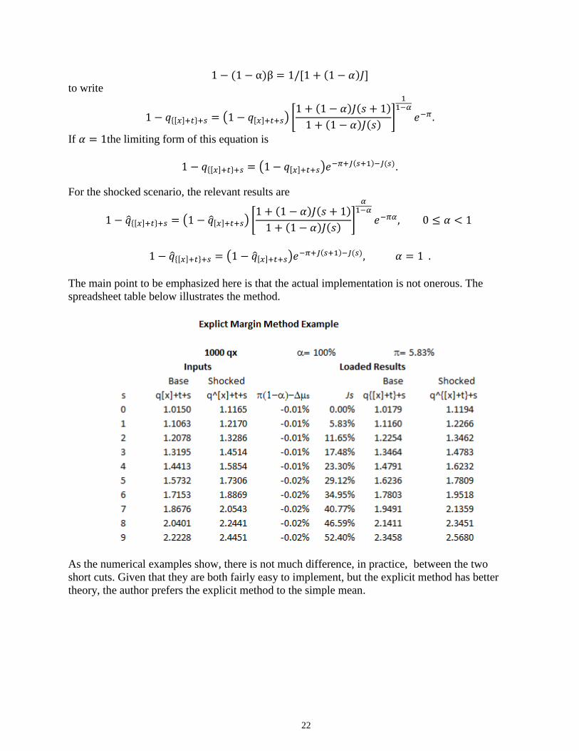
1 − ��{[𝑥]+𝑡}+𝑠 = (1 − ��[𝑥]+𝑡+𝑠)𝑒−𝜋+𝐽(𝑠+1)−𝐽(𝑠), 𝛼 = 1 .

The main point to be emphasized here is that the actual implementation is not onerous. The

spreadsheet table below illustrates the method.

As the numerical examples show, there is not much difference, in practice, between the two

short cuts. Given that they are both fairly easy to implement, but the explicit method has better

theory, the author prefers the explicit method to the simple mean.