Embed Size (px)
Citation preview
Doug Downey (adapted from Bryan Pardo, Northwestern University)
Machine Learning
Probability and Bayesian Networks
Doug Downey (adapted from Bryan Pardo, Northwestern University)
An Introduction
• Bayesian Decision Theory came long before Version Spaces, Decision Tree Learning and Neural Networks. It was studied in the field of Statistical Theory and more specifically, in the field of Pattern Recognition.
Doug Downey (adapted from Bryan Pardo, Northwestern University)
An Introduction
• Bayesian Decision Theory is at the basis of important learning schemes such as…– Naïve Bayes Classifier– Bayesian Belief Networks – EM Algorithm
• Bayesian Decision Theory is also useful as it provides a framework within which many non-Bayesian classifiers can be studied – See [Mitchell, Sections 6.3, 4,5,6].
Doug Downey (adapted from Bryan Pardo, Northwestern University)
Discrete Random Variables
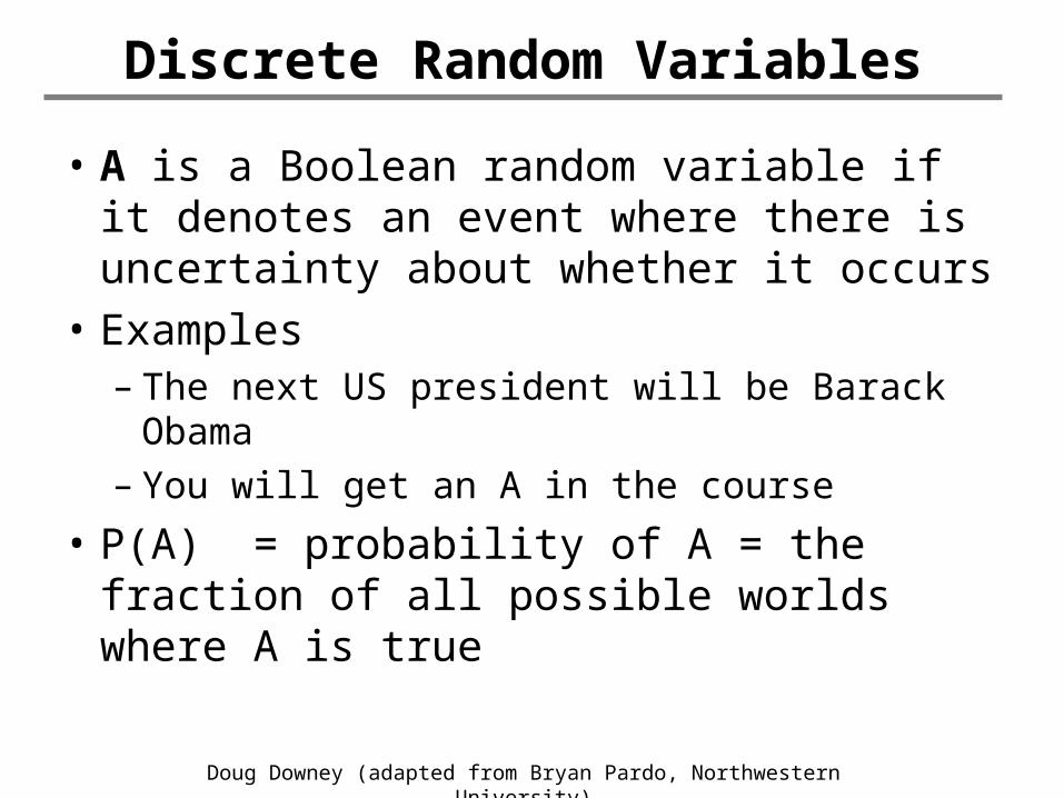
• A is a Boolean random variable if it denotes an event where there is uncertainty about whether it occurs
• Examples– The next US president will be Barack
Obama– You will get an A in the course
• P(A) = probability of A = the fraction of all possible worlds where A is true
Doug Downey (adapted from Bryan Pardo, Northwestern University)
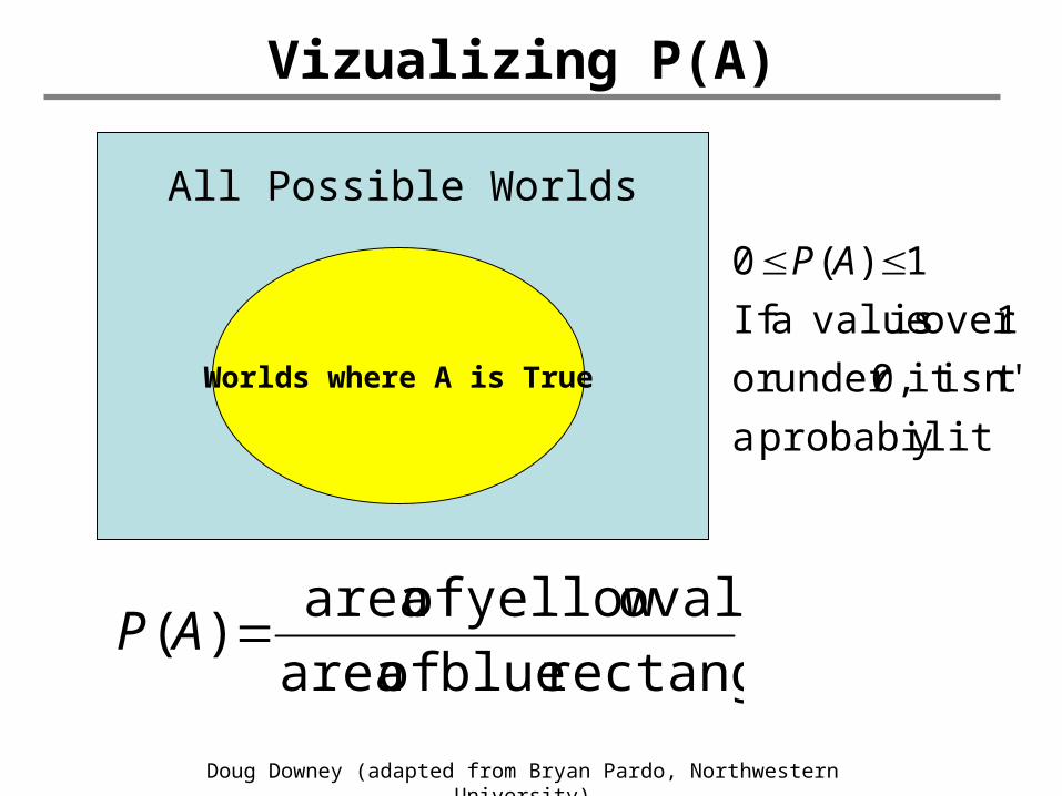
Vizualizing P(A)
rectangle blue of area
oval yellow of area)( AP
yprobabilit a
t isn'it 0,under or
1over is valuea If
1)(0 AP
All Possible Worlds
Worlds where A is True
rectangle blue of area
oval yellow of area)( AP
Doug Downey (adapted from Bryan Pardo, Northwestern University)
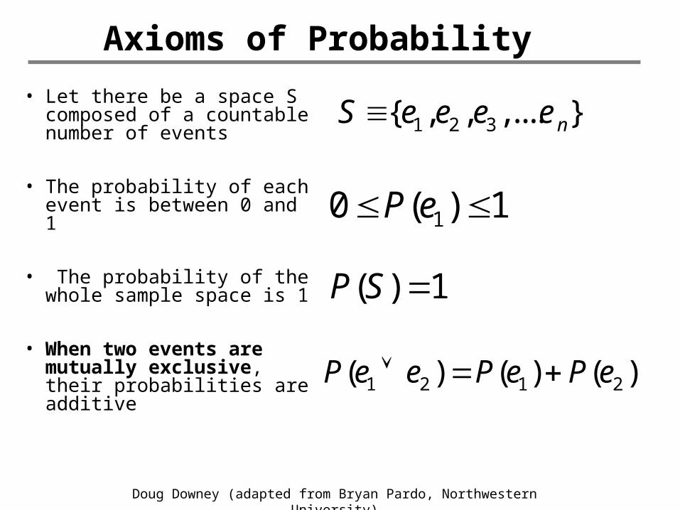
Axioms of Probability
• Let there be a space S composed of a countable number of events
• The probability of each event is between 0 and 1
• The probability of the whole sample space is 1
• When two events are mutually exclusive, their probabilities are additive
1 2 3{ , , ,.... }nS e e e e
1)(0 1 eP
1)( SP
)()()( 2121 ePePeeP
Doug Downey (adapted from Bryan Pardo, Northwestern University)
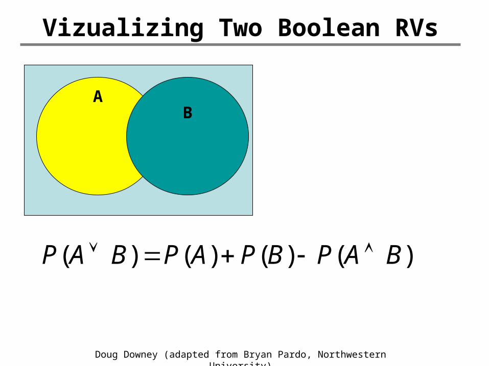
Vizualizing Two Boolean RVs
)()()()( BAPBPAPBAP
rectangle blue of area
oval yellow of area)( AP
AB
Doug Downey (adapted from Bryan Pardo, Northwestern University)
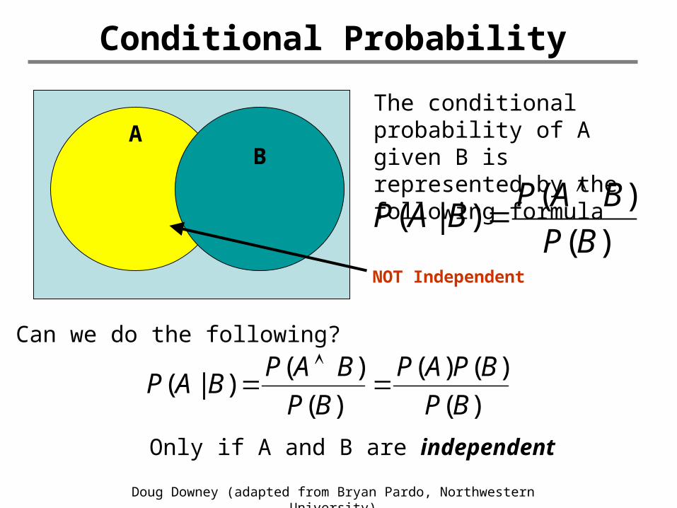
Conditional Probability
rectangle blue of area
oval yellow of area)( AP
)(
)()|(
BP
BAPBAP
AB
Can we do the following?
)(
)()(
)(
)()|(
BP
BPAP
BP
BAPBAP
Only if A and B are independent
The conditional probability of A given B is represented by the following formula
NOT Independent
Doug Downey (adapted from Bryan Pardo, Northwestern University)
Independence
• variables A and B are said to be independent if knowing the value of A gives you no knowledge about the likelihood of B…and vice-versa
P(A|B) = P(A) and P(B|A) = P(B)
Doug Downey (adapted from Bryan Pardo, Northwestern University)
An Example: Cards
• Take a standard deck of 52 cards. • On the first draw I pull the Ace of Spades. • I don’t replace the card.
– What is the probability I’ll pull the Ace of Spades on the second draw?
• Now, I replace the Ace after the 1st draw, shuffle, and draw again. – What is the chance I’ll draw the Ace of Spades
on the 2nd draw?
Discrete Random Variables
• A is a discrete random variable if it takes a countable number of distinct values
• Examples– Your grade G in the course– The number of heads k in n coin flips
• P(A=k) = the fraction of all possible worlds where A equals k
• Notation: PD(A = k) prob. relative to a distribution D
– Pfair grading(G = “A”), Pcheating(G = “A”)
Doug Downey (adapted from Bryan Pardo, Northwestern University)
Doug Downey (adapted from Bryan Pardo, Northwestern University)
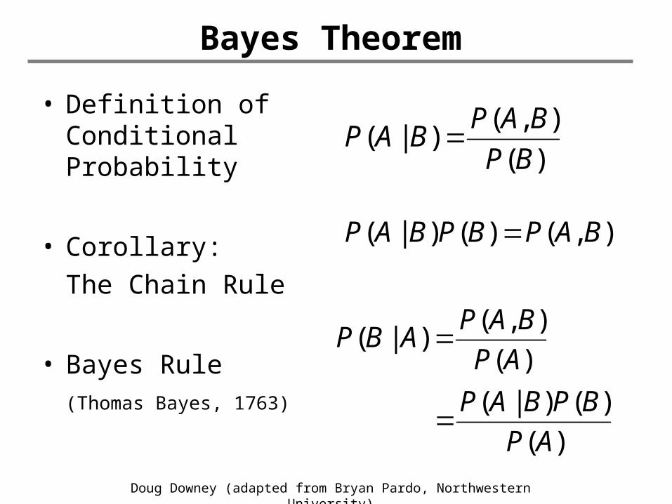
Bayes Theorem
• Definition of Conditional Probability
• Corollary: The Chain Rule
• Bayes Rule (Thomas Bayes, 1763)
),()()|( BAPBPBAP
)(
),()|(
BP
BAPBAP
)(
)()|(
)(
),()|(
AP
BPBAP
AP
BAPABP
ML in a Bayesian Framework
• Any ML technique can be expressed as reasoning about probabilities
• Goal: Find hypothesis h that is most probable given training data D
• Provides a more explicit way of describing & encoding our assumptions
Doug Downey (adapted from Bryan Pardo, Northwestern University)
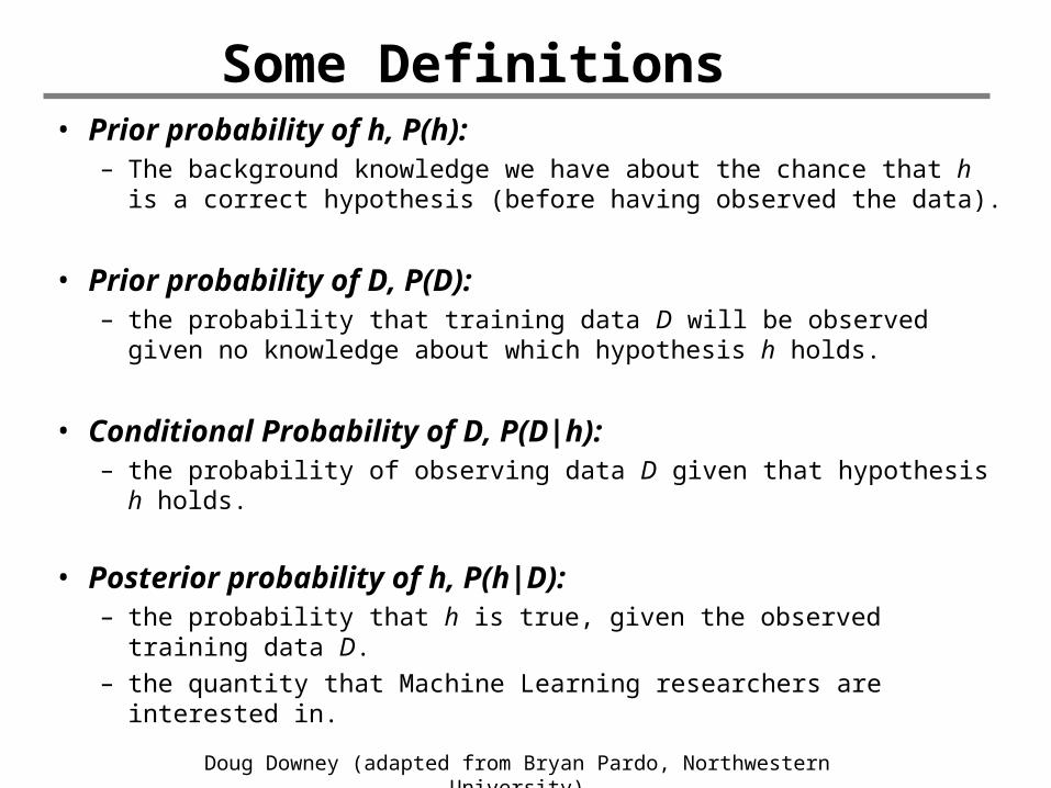
Some Definitions• Prior probability of h, P(h):
– The background knowledge we have about the chance that h is a correct hypothesis (before having observed the data).
• Prior probability of D, P(D): – the probability that training data D will be observed given no
knowledge about which hypothesis h holds.
• Conditional Probability of D, P(D|h): – the probability of observing data D given that hypothesis h
holds.
• Posterior probability of h, P(h|D): – the probability that h is true, given the observed training data
D. – the quantity that Machine Learning researchers are interested
in.
Doug Downey (adapted from Bryan Pardo, Northwestern University)
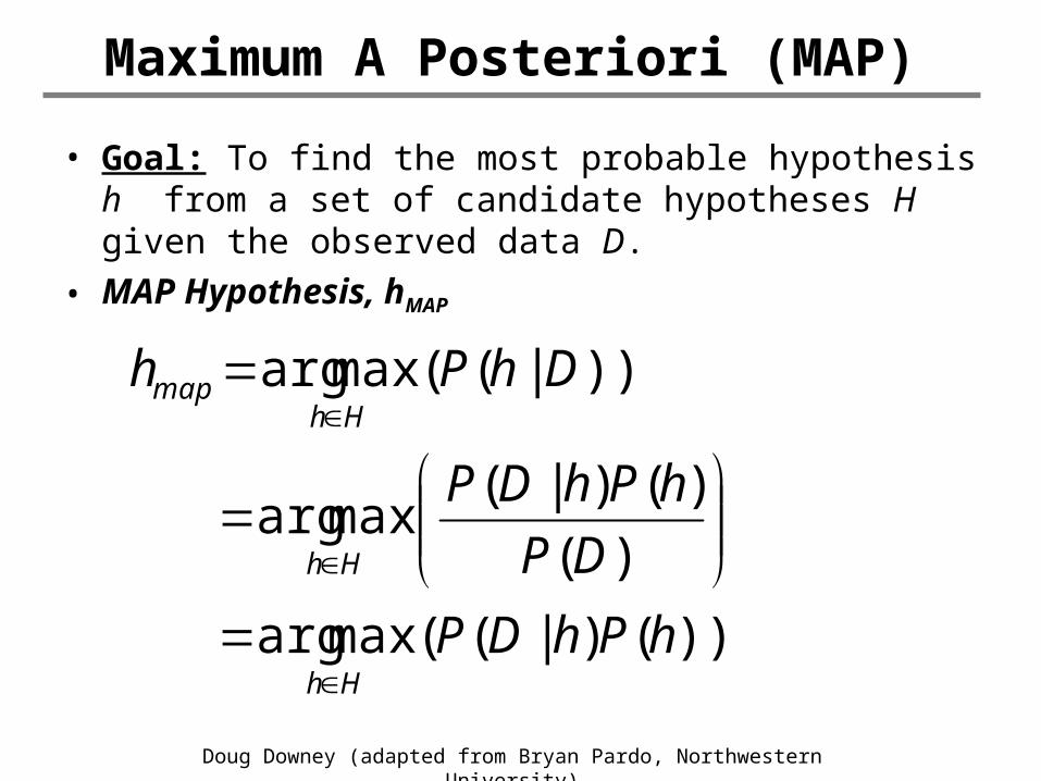
Maximum A Posteriori (MAP)
• Goal: To find the most probable hypothesis h from a set of candidate hypotheses H given the observed data D.
• MAP Hypothesis, hMAP
))()|((maxarg
)(
)()|(maxarg
))|((maxarg
hPhDP
DP
hPhDP
DhPh
Hh
Hh
Hhmap
Doug Downey (adapted from Bryan Pardo, Northwestern University)
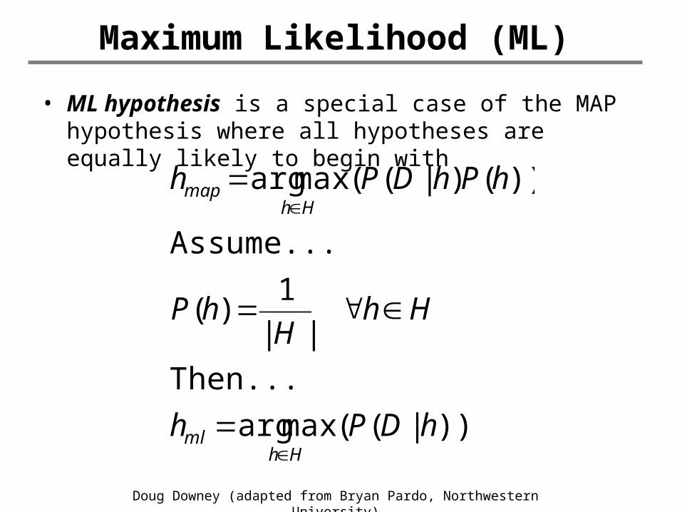
Maximum Likelihood (ML)
• ML hypothesis is a special case of the MAP hypothesis where all hypotheses are equally likely to begin with
))|((maxarg
Then...
||
1)(
Assume...
))()|((maxarg
hDPh
HhH
hP
hPhDPh
Hhml
Hhmap
Doug Downey (adapted from Bryan Pardo, Northwestern University)
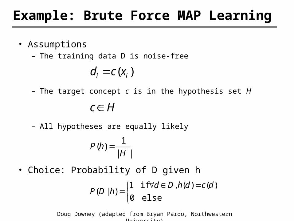
Example: Brute Force MAP Learning
• Assumptions– The training data D is noise-free
– The target concept c is in the hypothesis set H
– All hypotheses are equally likely
• Choice: Probability of D given h
)( ii xcd
Hc
||
1)(
HhP
else 0
)()( , if 1)|(
dcdhDdhDP
Doug Downey (adapted from Bryan Pardo, Northwestern University)
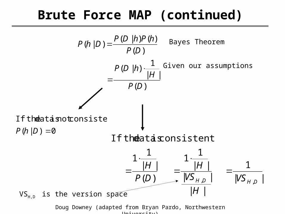
Brute Force MAP (continued)
)(||
1)|(
)(
)()|()|(
DPH
hDP
DP
hPhDPDhP
||
1
||
||||
11
)(||
11
consistent is data theIf
,, DHDH VSH
VSH
DPH
Bayes Theorem
Given our assumptions
0 )|(
consistentnot is data theIf
DhP
VSH,D is the version space
Doug Downey (adapted from Bryan Pardo, Northwestern University)
Find-S as MAP Learning
• We can characterize the FIND-S learner (chapter 2) in Bayesian terms – Again P(D | h) is 1 if h is consistent on D,
and 0 otherwise– P(h) increases with…
• specificity of h
– Then: MAP hypothesis = output of Find-S
Doug Downey (adapted from Bryan Pardo, Northwestern University)
Neural Nets in a Bayesian Framework
• Under certain assumptions regarding noise in the data, minimizing the mean squared error (what multilayer perceptrons do) corresponds to computing the maximum likelihood hypothesis.
Doug Downey (adapted from Bryan Pardo, Northwestern University)
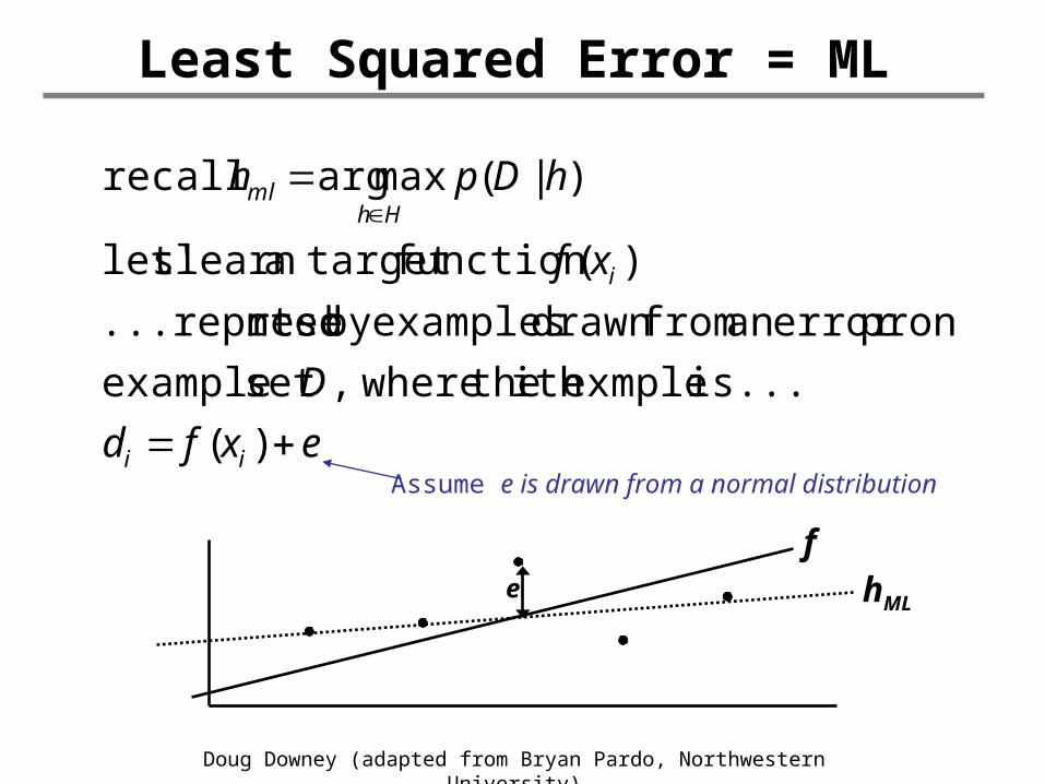
Least Squared Error = ML
exfd
D
xf
hDph
ii
i
Hhml
)(
is... exmpleith the where,set example
proneerror an fromdrawn examplesby nted...represe
)(function target alearn slet'
)|(maxarg recall
Assume e is drawn from a normal distribution
hML
fe
Doug Downey (adapted from Bryan Pardo, Northwestern University)
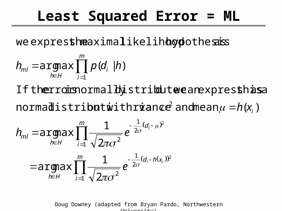
Least Squared Error = ML
m
i
xhd
Hh
m
i
d
Hhml
i
m
ii
Hhml
ii
i
e
eh
xh
hdph
1
2
1
2
1
2
1
2
2
1
2
2
2
1maxarg
2
1maxarg
)(mean and rianceon with vadistributi normal
a as thisexpresscan weddistributenormally iserror theIf
)|(maxarg
as hypothesis likelihood maximal theexpress we
Doug Downey (adapted from Bryan Pardo, Northwestern University)
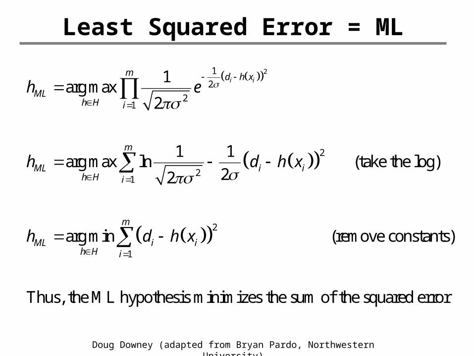
Least Squared Error = ML
21
2
21
2
21
2
1
1arg max
2
1 1arg max ln (take the log)
22
arg min (remove constants)
Thus, the ML hypothesis minimizes the
i im d h x
MLh H i
m
ML i ih H i
m
ML i ih H i
h e
h d h x
h d h x
sum of the squared error
Doug Downey (adapted from Bryan Pardo, Northwestern University)
Decision Trees in Bayes Framework
• Decent choice for P(h): simpler hypotheses have higher probability– Occam’s razor
• This can be encoded in terms of finding the “Minimum Description Length” encoding– Provides a way to “trade off” hypothesis
size for training error– Potentially prevents overfitting
Doug Downey (adapted from Bryan Pardo, Northwestern University)
Most Compact Coding
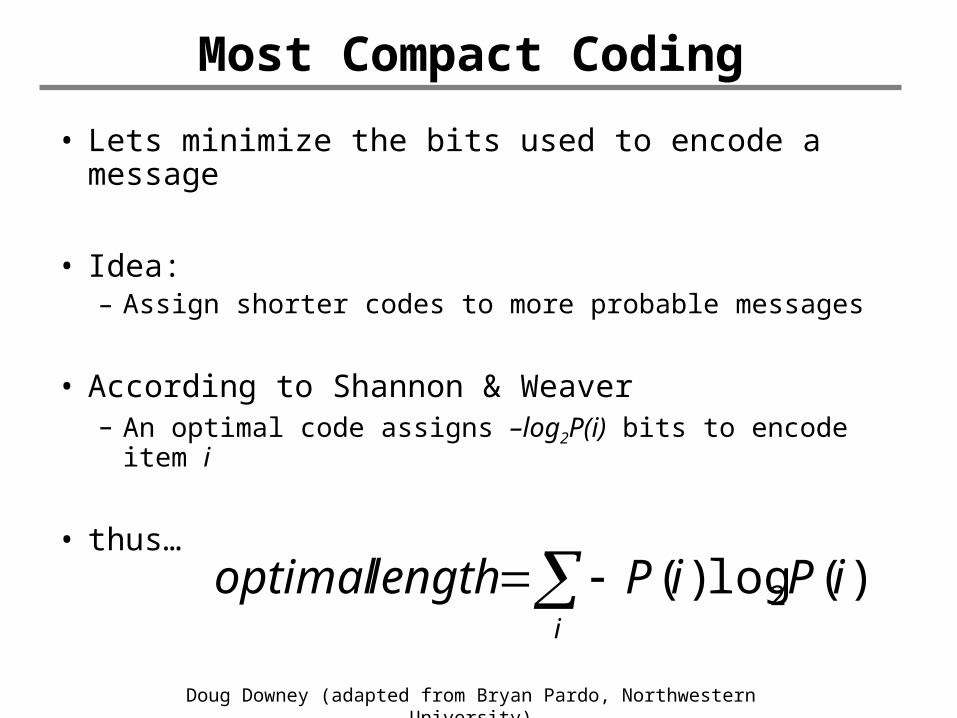
• Lets minimize the bits used to encode a message
• Idea: – Assign shorter codes to more probable messages
• According to Shannon & Weaver– An optimal code assigns –log2P(i) bits to encode item i
• thus…
)(log)( 2 iPiPlengthoptimali
Doug Downey (adapted from Bryan Pardo, Northwestern University)
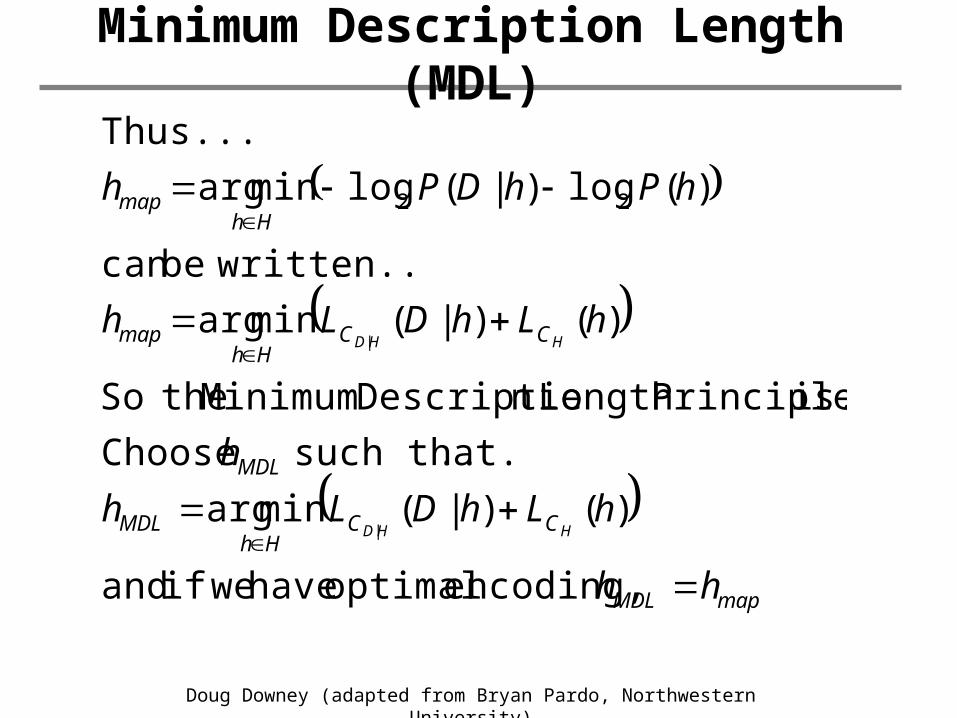
Minimum Description Length (MDL)
|
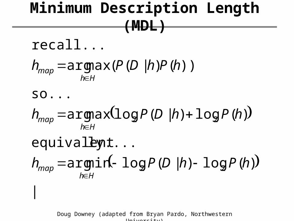
)(log)|(logminarg
ly....equivalent
)(log)|(logmaxarg
so...
))()|((maxarg
recall...
22
22
hPhDPh
hPhDPh
hPhDPh
Hhmap
Hhmap
Hhmap
Doug Downey (adapted from Bryan Pardo, Northwestern University)
Minimum Description Length (MDL)
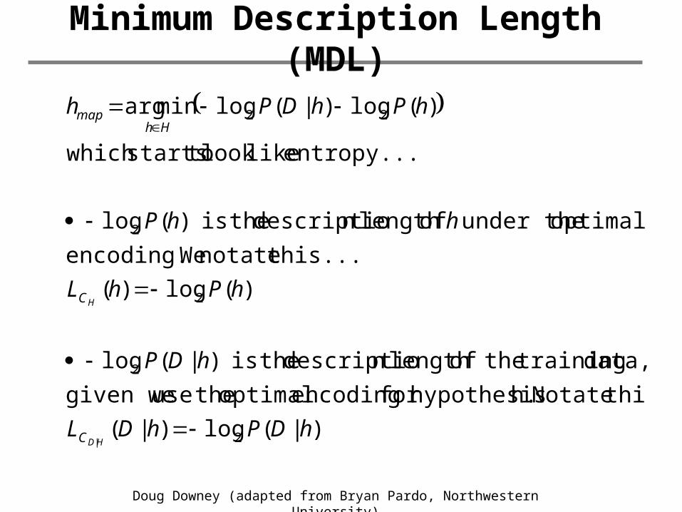
)|(log)|(
this..Notate h. hypothesisfor encoding optimal theuse given we
data, training theoflength n descriptio theis )|(log
)(log)(
this...notate Weencoding.
optimal under the oflength n descriptio theis )(log
entropy... likelook tostartswhich
)(log)|(logminarg
2
2
2
2
22
|hDPhDL
hDP
hPhL
hhP
hPhDPh
HD
H
C
C
Hhmap
Doug Downey (adapted from Bryan Pardo, Northwestern University)
Minimum Description Length (MDL)
mapMDL
CCHh
MDL
MDL
CCHh
map
Hhmap
hh
hLhDLh
h
hLhDLh
hPhDPh
HHD
HHD
encoding, optimal have weif and
)()|(minarg
..such that. Choose
is... PrincipleLength n Descriptio Minimum theSo
)()|(minarg
. written..becan
)(log)|(logminarg
Thus...
|
|
22
Doug Downey (adapted from Bryan Pardo, Northwestern University)
What does all that mean?
• The “optimal” hypothesis is the one that is the smallest when we count…– How long the hypothesis description
must be– How long the data description must be,
given the hypothesis• Key idea: since we’re given h, we need only
encode h’s mistakes
Doug Downey (adapted from Bryan Pardo, Northwestern University)
What does all that mean?
• If the hypothesis is perfect, we don’t need to encode any data.
• For each misclassification, we must– say which item is misclassified
• Takes log2m bits, where m = size of the dataset
– Say what the right classification is• Takes log2k bits, where k = number of
classes
Doug Downey (adapted from Bryan Pardo, Northwestern University)
The best MDL hypothesis
• The best hypothesis is the best tradeoff between– Complexity of the hypothesis description– Number of times we have to tell people
where it screwed up.
Doug Downey (adapted from Bryan Pardo, Northwestern University)
Is MDL always MAP?
• Only given significant assumptions:– If we know a representation scheme
such that size of h in H is -log2P(h)
– Likewise, the size of the exception representation must be –log2P(D|h)
– THEN• MDL = MAP
Doug Downey (adapted from Bryan Pardo, Northwestern University)
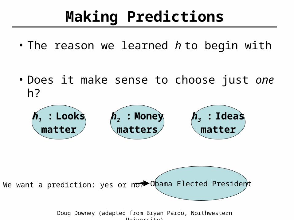
Making Predictions
• The reason we learned h to begin with
• Does it make sense to choose just one h?
h1 : Looksmatter
Obama Elected PresidentWe want a prediction: yes or no?
h2 : Moneymatters
h3 : Ideasmatter
Doug Downey (adapted from Bryan Pardo, Northwestern University)
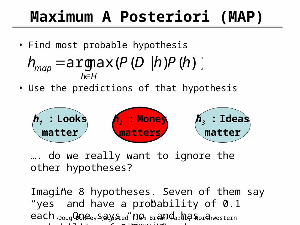
Maximum A Posteriori (MAP)
• Find most probable hypothesis
• Use the predictions of that hypothesis
))()|((maxarg hPhDPhHh
map
h1 : Looksmatter
h2 : Moneymatters
h3 : Ideasmatter
…. do we really want to ignore the other hypotheses?
Imagine 8 hypotheses. Seven of them say “yes” and have a probability of 0.1 each. One says “no” and has a probability of 0.3. Who do you believe?
Doug Downey (adapted from Bryan Pardo, Northwestern University)
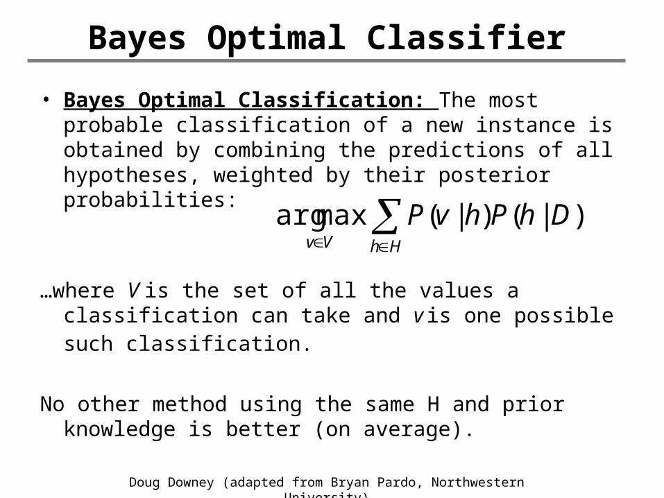
Bayes Optimal Classifier
• Bayes Optimal Classification: The most probable classification of a new instance is obtained by combining the predictions of all hypotheses, weighted by their posterior probabilities:
…where V is the set of all the values a classification can take and v is one possible such classification.
No other method using the same H and prior knowledge is better (on average).
HhVv
DhPhvP )|()|(maxarg
Doug Downey (adapted from Bryan Pardo, Northwestern University)
Naïve Bayes Classifier
• Unfortunately, Bayes Optimal Classifier is usually too costly to apply! ==> Naïve Bayes Classifier
We’ll be seeing more of these…
Doug Downey (adapted from Bryan Pardo, Northwestern University)
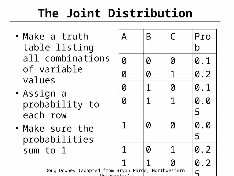
The Joint Distribution
• Make a truth table listing all combinations of variable values
• Assign a probability to each row
• Make sure the probabilities sum to 1
A B C Prob
0 0 0 0.1
0 0 1 0.2
0 1 0 0.1
0 1 1 0.05
1 0 0 0.05
1 0 1 0.2
1 1 0 0.25
1 1 1 0.05
Doug Downey (adapted from Bryan Pardo, Northwestern University)
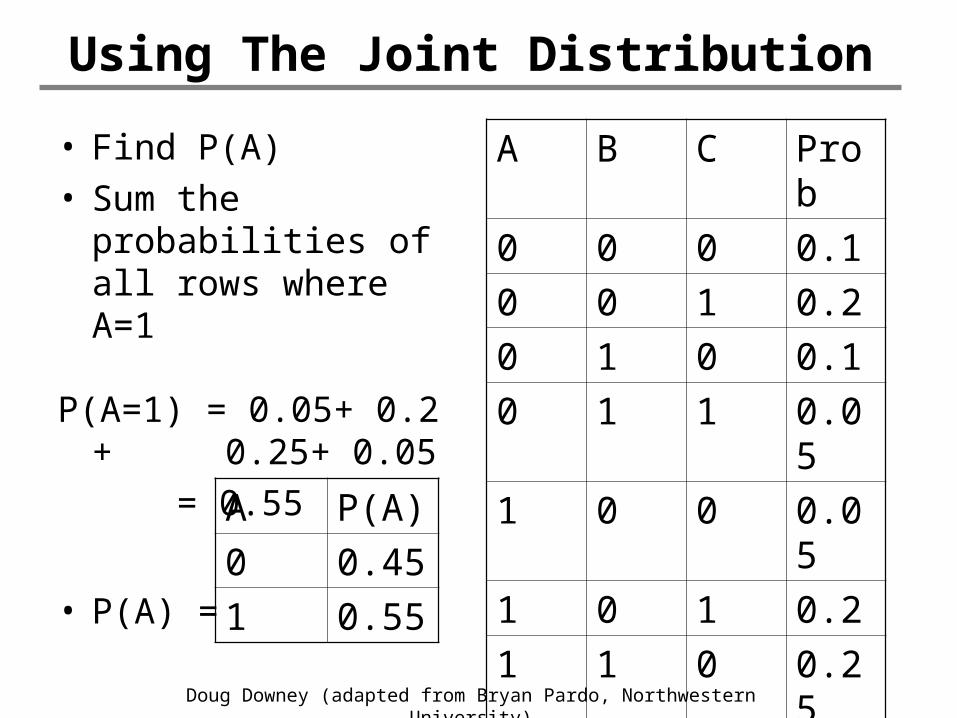
Using The Joint Distribution
• Find P(A)• Sum the
probabilities of all rows where A=1
P(A=1) = 0.05+ 0.2 + 0.25+ 0.05 = 0.55
• P(A) =
A B C Prob
0 0 0 0.1
0 0 1 0.2
0 1 0 0.1
0 1 1 0.05
1 0 0 0.05
1 0 1 0.2
1 1 0 0.25
1 1 1 0.05
A P(A)
0 0.45
1 0.55
Doug Downey (adapted from Bryan Pardo, Northwestern University)
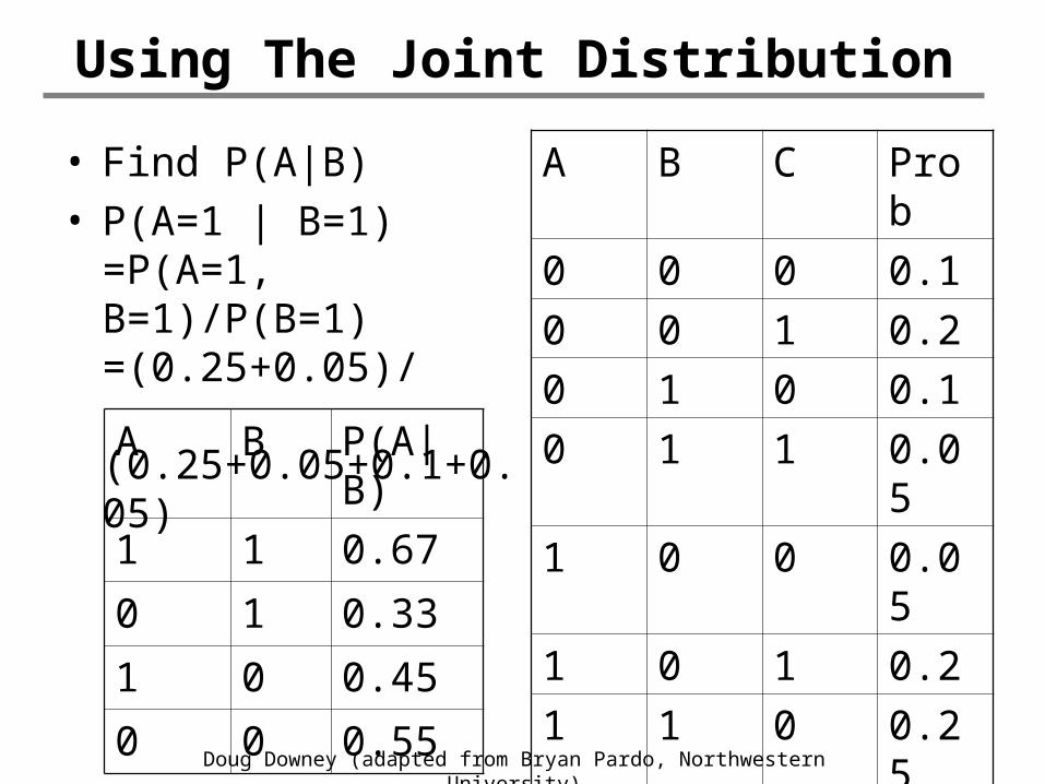
Using The Joint Distribution
• Find P(A|B)• P(A=1 | B=1)
=P(A=1, B=1)/P(B=1)=(0.25+0.05)/ (0.25+0.05+0.1+0.05)
A B C Prob
0 0 0 0.1
0 0 1 0.2
0 1 0 0.1
0 1 1 0.05
1 0 0 0.05
1 0 1 0.2
1 1 0 0.25
1 1 1 0.05
A B P(A|B)
1 1 0.67
0 1 0.33
1 0 0.45
0 0 0.55
Doug Downey (adapted from Bryan Pardo, Northwestern University)
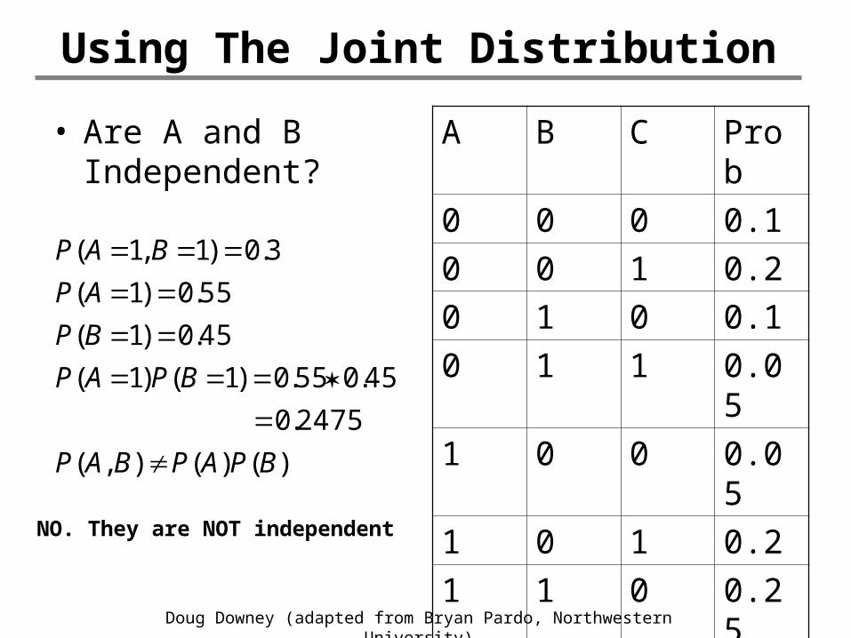
Using The Joint Distribution
• Are A and B Independent?
A B C Prob
0 0 0 0.1
0 0 1 0.2
0 1 0 0.1
0 1 1 0.05
1 0 0 0.05
1 0 1 0.2
1 1 0 0.25
1 1 1 0.05
)()(),(
2475.0
45.055.0)1()1(
45.0)1(
55.0)1(
3.0)1,1(
BPAPBAP
BPAP
BP
AP
BAP
NO. They are NOT independent
Doug Downey (adapted from Bryan Pardo, Northwestern University)
Why not use the Joint Distribution?
• Given m boolean variables, we need to estimate 2m-1 values.
• 20 yes-no questions = a million values
• How do we get around this combinatorial explosion? – Assume independence of variables!!
Doug Downey (adapted from Bryan Pardo, Northwestern University)
…back to Independence
• The probability I have an apple in my lunch bag is independent of the probability of a blizzard in Japan.
• This is DOMAIN Knowledge, typically supplied by the problem designer
)()|( APBAP
Doug Downey (adapted from Bryan Pardo, Northwestern University)
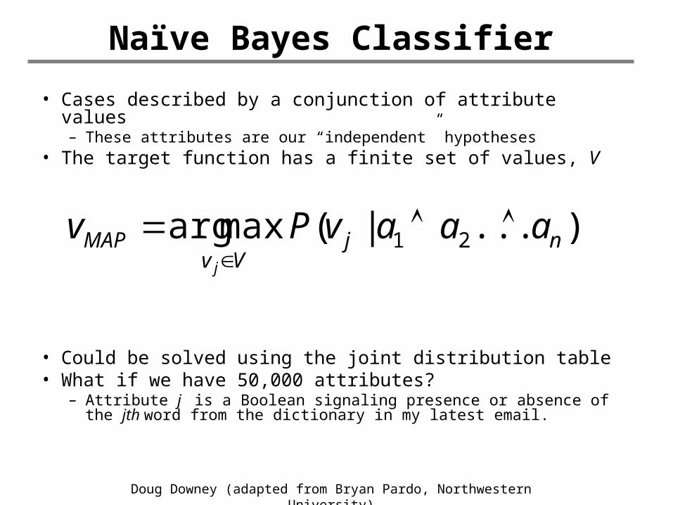
Naïve Bayes Classifier
• Cases described by a conjunction of attribute values– These attributes are our “independent” hypotheses
• The target function has a finite set of values, V
• Could be solved using the joint distribution table• What if we have 50,000 attributes?
– Attribute j is a Boolean signaling presence or absence of the jth word from the dictionary in my latest email.
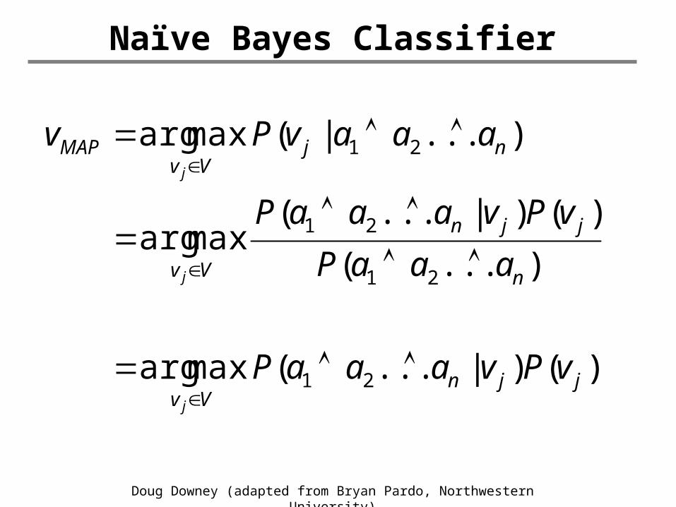
)...|(maxarg 21 njVv
MAP aaavPvj
Doug Downey (adapted from Bryan Pardo, Northwestern University)
Naïve Bayes Classifier
)()|...(maxarg
)...(
)()|...(maxarg
)...|(maxarg
21
21
21
21
jjnVv
n
jjn
Vv
njVv
MAP
vPvaaaP
aaaP
vPvaaaP
aaavPv
j
j
j
Doug Downey (adapted from Bryan Pardo, Northwestern University)
Naïve Bayes Continued
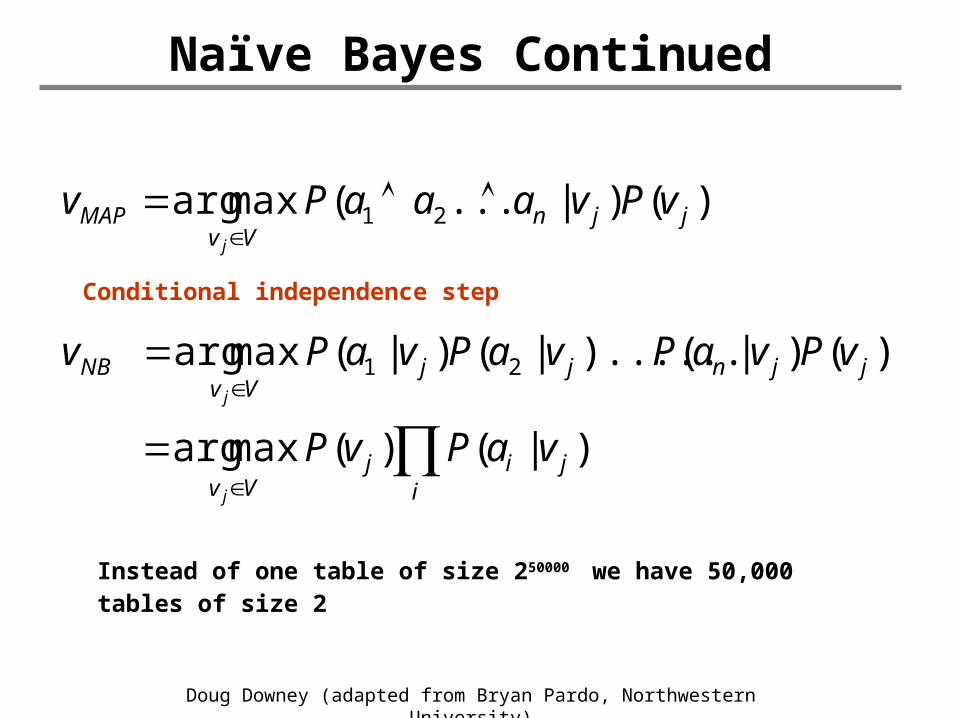
)|()(maxarg
)()|()......|()|(maxarg
)()|...(maxarg
21
21
ji
ijVv
jjnjjVv
NB
jjnVv
MAP
vaPvP
vPvaPvaPvaPv
vPvaaaPv
j
j
j
Conditional independence step
Instead of one table of size 250000 we have 50,000 tables of size 2
Doug Downey (adapted from Bryan Pardo, Northwestern University)
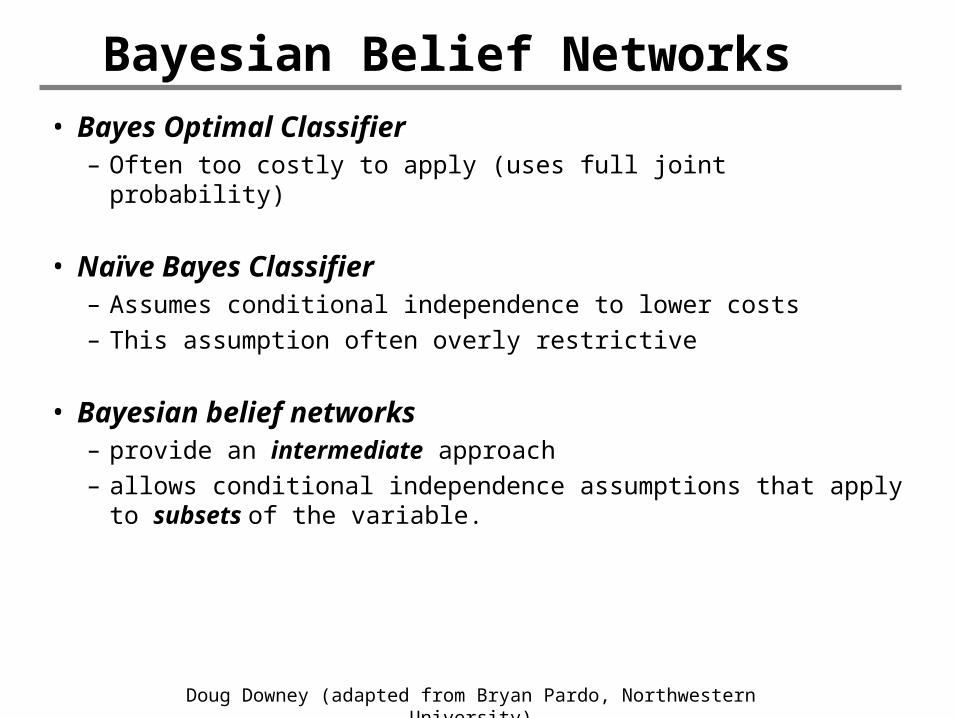
Bayesian Belief Networks
• Bayes Optimal Classifier – Often too costly to apply (uses full joint probability)
• Naïve Bayes Classifier – Assumes conditional independence to lower costs – This assumption often overly restrictive
• Bayesian belief networks – provide an intermediate approach – allows conditional independence assumptions that apply
to subsets of the variable.
Doug Downey (adapted from Bryan Pardo, Northwestern University)
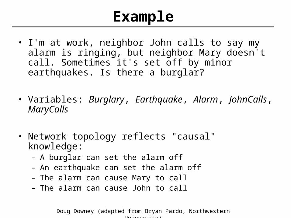
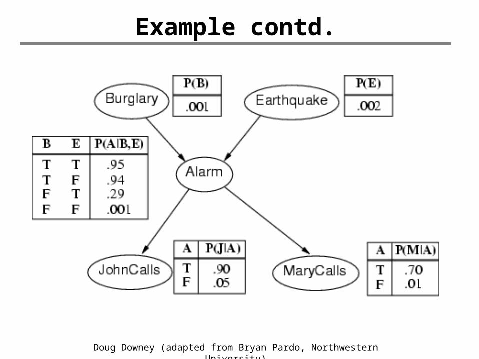
Example
• I'm at work, neighbor John calls to say my alarm is ringing, but neighbor Mary doesn't call. Sometimes it's set off by minor earthquakes. Is there a burglar?
• Variables: Burglary, Earthquake, Alarm, JohnCalls, MaryCalls
• Network topology reflects "causal" knowledge:– A burglar can set the alarm off– An earthquake can set the alarm off– The alarm can cause Mary to call– The alarm can cause John to call
Doug Downey (adapted from Bryan Pardo, Northwestern University)
Example contd.
Doug Downey (adapted from Bryan Pardo, Northwestern University)
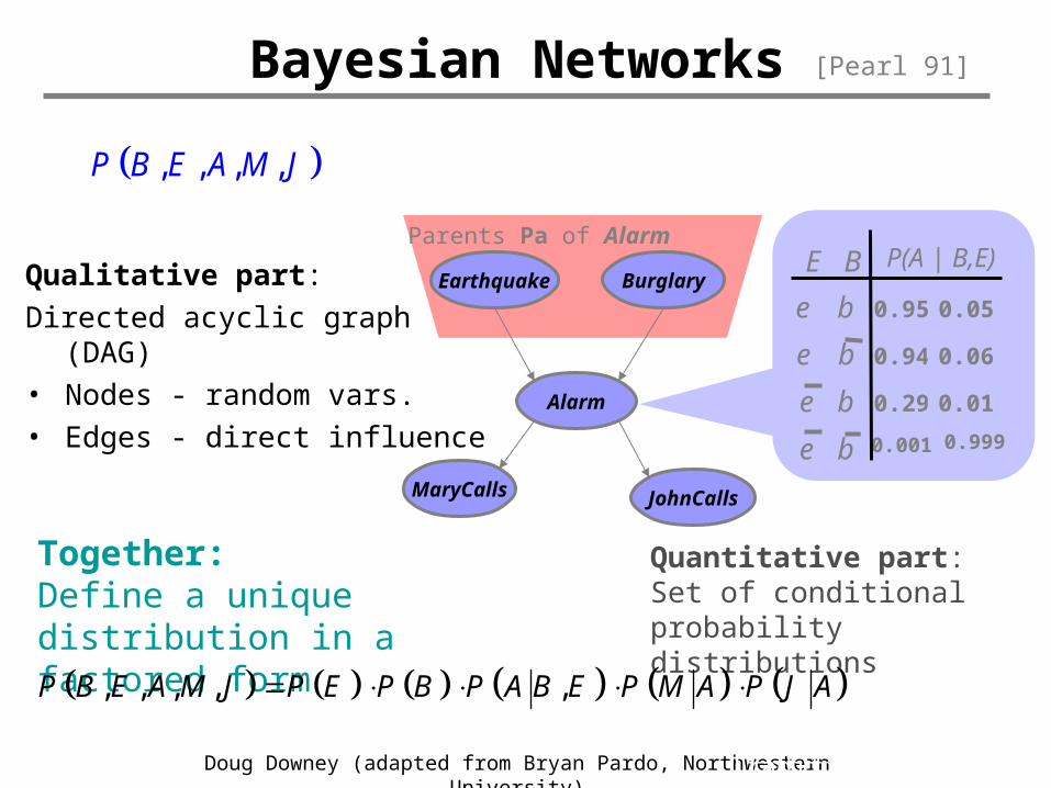
Qualitative part: Directed acyclic graph (DAG)• Nodes - random vars. • Edges - direct influence
Quantitative part: Set of conditional probability distributions
0.95 0.05
e
b
e
0.94 0.06
0.001 0.999
0.29 0.01
be
b
b
e
BE P(A | B,E)
[Pearl 91]
Parents Pa of Alarm
Bayesian Networks
Earthquake
JohnCalls
Burglary
Alarm
MaryCalls
Together:Define a unique distribution in a factored form
, , , , ,P B E A M J P E P B P A B E P M A P J A
, , , ,P B E A M J
Traditional Approaches
Doug Downey (adapted from Bryan Pardo, Northwestern University)
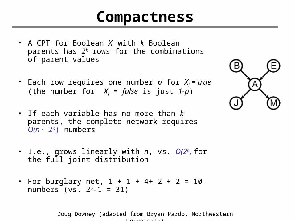
Compactness
• A CPT for Boolean Xi with k Boolean parents has 2k rows for the combinations of parent values
• Each row requires one number p for Xi = true(the number for Xi = false is just 1-p)
• If each variable has no more than k parents, the complete network requires O(n · 2k) numbers
• I.e., grows linearly with n, vs. O(2n) for the full joint distribution
• For burglary net, 1 + 1 + 4+ 2 + 2 = 10 numbers (vs. 25-1 = 31)
Doug Downey (adapted from Bryan Pardo, Northwestern University)
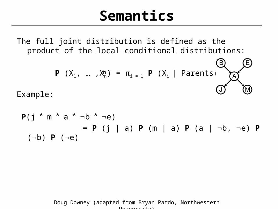
Semantics
The full joint distribution is defined as the product of the local conditional distributions:
P (X1, … ,Xn) = πi = 1 P (Xi | Parents(Xi))
Example:
P(j m a b e)= P (j | a) P (m | a) P (a | b, e) P (b) P
(e)
n
Doug Downey (adapted from Bryan Pardo, Northwestern University)
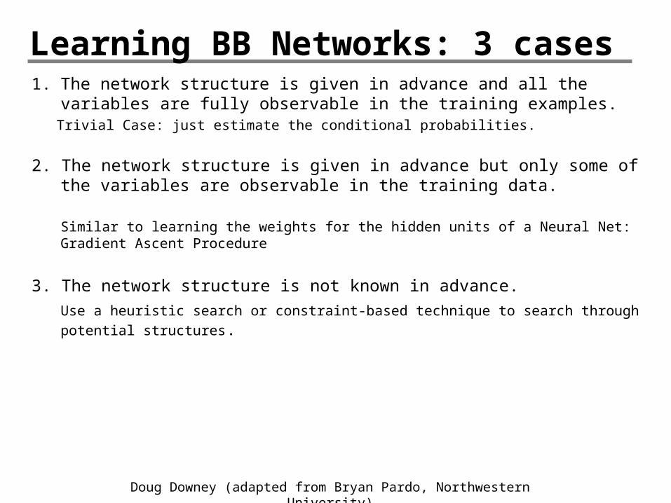
Learning BB Networks: 3 cases1. The network structure is given in advance and all the variables
are fully observable in the training examples. Trivial Case: just estimate the conditional probabilities.
2. The network structure is given in advance but only some of the variables are observable in the training data.
Similar to learning the weights for the hidden units of a Neural Net: Gradient Ascent Procedure
3. The network structure is not known in advance. Use a heuristic search or constraint-based technique to search through potential structures.
Doug Downey (adapted from Bryan Pardo, Northwestern University)
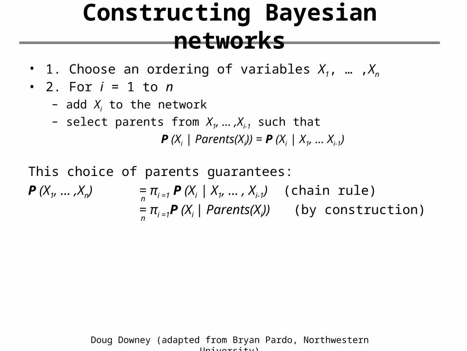
Constructing Bayesian networks
• 1. Choose an ordering of variables X1, … ,Xn
• 2. For i = 1 to n– add Xi to the network– select parents from X1, … ,Xi-1 such that
P (Xi | Parents(Xi)) = P (Xi | X1, ... Xi-1)
This choice of parents guarantees:P (X1, … ,Xn) = πi =1 P (Xi | X1, … , Xi-1) (chain rule)
= πi =1P (Xi | Parents(Xi)) (by construction)n
n
Doug Downey (adapted from Bryan Pardo, Northwestern University)
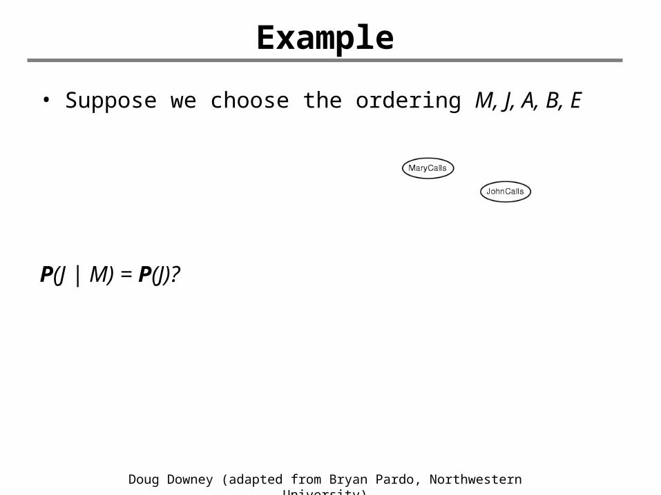
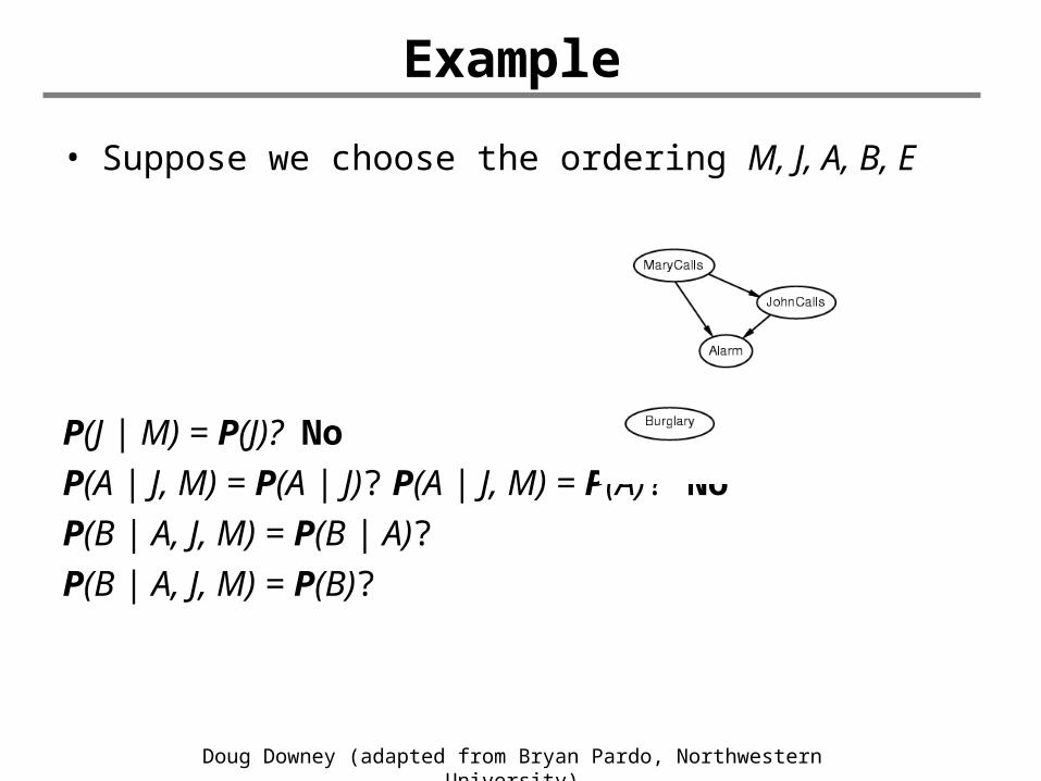
• Suppose we choose the ordering M, J, A, B, E
P(J | M) = P(J)?
Example
Doug Downey (adapted from Bryan Pardo, Northwestern University)
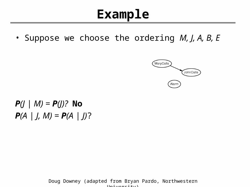
• Suppose we choose the ordering M, J, A, B, E
P(J | M) = P(J)? NoP(A | J, M) = P(A | J)?
Example
Doug Downey (adapted from Bryan Pardo, Northwestern University)
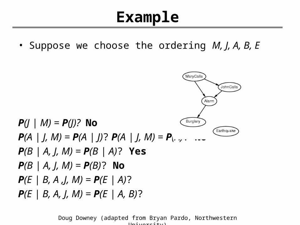
• Suppose we choose the ordering M, J, A, B, E
P(J | M) = P(J)? NoP(A | J, M) = P(A | J)? P(A | J, M) = P(A)? NoP(B | A, J, M) = P(B | A)? P(B | A, J, M) = P(B)?
Example
Doug Downey (adapted from Bryan Pardo, Northwestern University)
• Suppose we choose the ordering M, J, A, B, E
P(J | M) = P(J)? NoP(A | J, M) = P(A | J)? P(A | J, M) = P(A)? NoP(B | A, J, M) = P(B | A)? YesP(B | A, J, M) = P(B)? NoP(E | B, A ,J, M) = P(E | A)?P(E | B, A, J, M) = P(E | A, B)?
Example
Doug Downey (adapted from Bryan Pardo, Northwestern University)
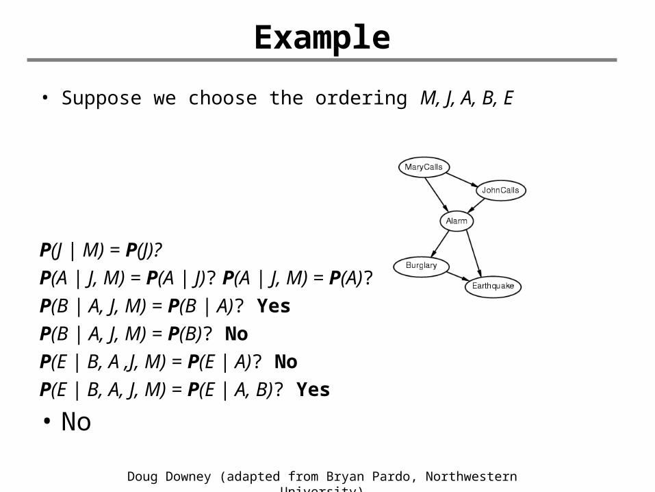
• Suppose we choose the ordering M, J, A, B, E
P(J | M) = P(J)?P(A | J, M) = P(A | J)? P(A | J, M) = P(A)? NoP(B | A, J, M) = P(B | A)? YesP(B | A, J, M) = P(B)? NoP(E | B, A ,J, M) = P(E | A)? NoP(E | B, A, J, M) = P(E | A, B)? Yes
• No
Example
Doug Downey (adapted from Bryan Pardo, Northwestern University)
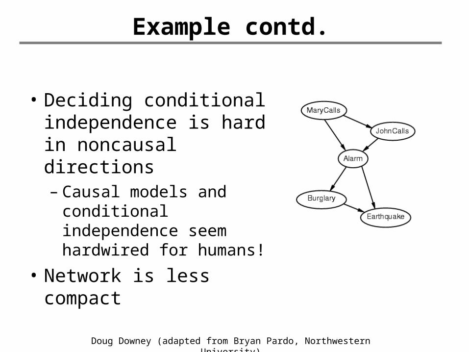
Example contd.
• Deciding conditional independence is hard in noncausal directions– Causal models and
conditional independence seem hardwired for humans!
• Network is less compact
Doug Downey (adapted from Bryan Pardo, Northwestern University)
Inference in BB Networks
• A Bayesian Network can be used to compute the probability distribution for any subset of network variables given the values or distributions for any subset of the remaining variables.
• Unfortunately, exact inference of probabilities in general for an arbitrary Bayesian Network is known to be NP-hard (#P-complete)
• In theory, approximate techniques (such as Monte Carlo Methods) can also be NP-hard, though in practice, many such methods are shown to be useful.
Doug Downey (adapted from Bryan Pardo, Northwestern University)
Expectation Maximization Algorithm
• Learning unobservable relevant variables
• Example:Assume that data points have been uniformly generated from k distinct Gaussian with the same known variance. The problem is to output a hypothesis h=<1, 2 ,.., k> that describes the means of each of the k distributions. In particular, we are looking for a maximum likelihood hypothesis for these means.
• We extend the problem description as follows: for each point xi, there are k hidden variables zi1,..,zik such that zil=1 if xi was generated by normal distribution l and ziq= 0 for all ql.
Doug Downey (adapted from Bryan Pardo, Northwestern University)
The EM Algorithm (Cont’d)• An arbitrary initial hypothesis h=<1, 2 ,.., k> is chosen.
• The EM Algorithm iterates over two steps:
– Step 1 (Estimation, E): Calculate the expected value E[zij] of each hidden variable zij, assuming that the current hypothesis h=<1, 2 ,.., k> holds.
– Step 2 (Maximization, M): Calculate a new maximum likelihood hypothesis h’=<1’, 2’ ,.., k’>,
assuming the value taken on by each hidden variable zij is its expected value E[zij] calculated in step 1.
Then replace the hypothesis h=<1, 2 ,.., k> by the new hypothesis h’=<1’, 2’ ,.., k’> and iterate.
The EM Algorithm can be applied to more general problems
Doug Downey (adapted from Bryan Pardo, Northwestern University)
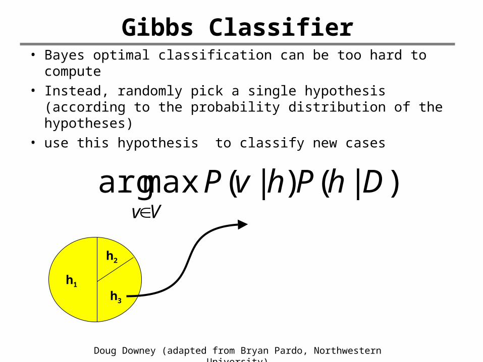
Gibbs Classifier• Bayes optimal classification can be too hard to
compute• Instead, randomly pick a single hypothesis (according
to the probability distribution of the hypotheses) • use this hypothesis to classify new cases
)|()|(maxarg DhPhvPVv
h1
h3
h2