Embed Size (px)
Citation preview

DOUBLY-FED INDUCTION MACHINE FOR VARIABLE SPEED ENERGY CONVERSION APPLICATIONS
Yongzheng Zhang
Department of Electrical and Computer Engineering McGill University
Montreal, Quebec, Canada
September 2012
A thesis submitted to The Faculty of Graduate Studies and Research
In partial fulfillment of the requirements for the degree of PhD of Engineering
© Yongzheng Zhang, 2012

i
Abstract
After decades of development, the wind energy industry is now supplying 10% to
20% of power in electric utilities. At present Doubly-Fed Induction Generators (DFIG)
are one of the most widely used generators in wind farms. The research of this thesis
advances the methods of controlling DFIGs by presenting:
(i) a non-mechanical (sensorless) method of determining accurate rotor speed and
rotor position which are essential in implementing decoupled P-Q control;
(ii) a method of autonomous frequency control whereby an islanded wind farm
does not have to shut down but continues to operate as standby ready to assist the utility
grid in fast restoration;
(iii) a method of mitigating the problem of power imbalance at the initial period
of islanding by using pitch control to spill excess wind power.
The thesis also examines what economical adaptation is required to make the
Doubly-Fed Induction Generator, which has the advanced controllers designed for wind
power application, marketable as Doubly-Fed Induction Motor.
Research is based on theoretical analysis, validated by digital simulation. A
prototype DFIG 5hp experimental platform, which has been built and tested, provides
experimental verification to claims.

ii
Résumé
Après des décennies de développement, l’industrie de l’énergie éolienne fournit
maintenant de 10% à 20% de la puissance produite dans les réseaux électriques.
Présentement, les alternateurs asynchrones à double alimentation (DFIG) sont parmi les
alternateurs les plus utilisés dans les parcs éoliens. La recherche de cette thèse avance les
méthodes de contrôle des DFIGs par la présentation:
(i) d’une méthode non-mécanique (sans capteur de mesure) afin de déterminer
précisément la vitesse et la position du rotor, qui sont essentielles dans l’implémentation
de contrôle découplée P-Q;
(ii) d’une méthode de contrôle autonome de la fréquence par quoi un parc éolien
îloté n’a pas à interrompre sa production mais il peut continuer à fonctionner en attente
pour aider le réseau électrique à une restauration rapide.
(iii) D’une méthode pour limiter le problème de déséquilibre de puissance au
début de l’îlotage en utilisant l’angle d’attaque de l’éolienne pour évacuer l’excédent de
la puissance éolienne.
Cette thèse examine aussi l’adaptation économique requise pour rendre
l’alternateur asynchrone à double alimentation, qui contient les contrôleurs conçus pour
l’application éolienne, commercialisable comme moteur asynchrone à double
alimentation.
La recherche est basée sur l’analyse théorique, validée par simulation digitale.
Une plateforme prototype d’un DFIG de 5hp, qui a été construite et testée, fournit la
vérification expérimentale des résultats de la recherche.

iii
Acknowledgements
I would like to express my sincere gratitude to all those who gave me the
possibility to complete this thesis. I am deeply indebted to my supervisor Professor Boon-
Teck Ooi, whose direction, suggestions and encouragement helped me in all the time of
research. I am also deeply grateful to Professor Geza Joos for his important support
throughout this work.
I wish to express my warm and sincere thanks to Dr. Bakari Mwiniwiwa of the
University of Dar-es-Salaam, Tanzania for his valuable advice and guidance.
My special thanks to Dr. Hadi Banakar for his knowledgeable assistance and
kindness for the study.
I would like to express my extended and special thanks to my family for their
support.

iv
Table of Contents
Abstract ............................................................................................................................... i Résumé ............................................................................................................................... ii Acknowledgements .......................................................................................................... iii List of Figures .................................................................................................................. vii List of Tables .................................................................................................................... ix List of Symbols ...................................................................................................................x List of Acronyms .............................................................................................................. xi Chapter 1: Introduction ....................................................................................................1
1.1 Research Background ..........................................................................................1 1.1.1 Fact of Wind Power in Canada .......................................................................1 1.1.2 Wind Energy Research at McGill University .................................................2 1.1.3 Wind Energy Conversion System ...................................................................2
1.2 Research Objective ..............................................................................................5 1.3 Methodology ........................................................................................................6 1.4 Organization and Contributions of Thesis ...........................................................7 1.5 Claims to Originality..........................................................................................13
Chapter 2: DFIG with Speed and Position Sensorless Control for Wind Power Generation ............................................................................................................14
2.1 Introduction ........................................................................................................14 2.2 Background ........................................................................................................15
2.2.1 Induction Machine in a-b-c Frame ...............................................................15 2.2.2 Reference Frame Transformation .................................................................18 2.2.3 Induction Machine Model in γ-δ Reference Frame ......................................19 2.2.4 Decoupled P-Q Control with DFIG ..............................................................22
2.3 Rotor Position Phase Lock Loop .......................................................................25 2.3.1 Introduction ...................................................................................................25 2.3.2 Rotor Position PLL .......................................................................................26 2.3.3 Robustness with Respect to Noise and Double PLL ....................................30 2.3.4 Robustness with respect to Parameters of DFIG ..........................................34 2.3.5 Design Considerations ..................................................................................34 2.3.6 Proofs of Speed and Position Tracking by Simulations ................................35
2.4 Rotor Position PLL for Decoupled P-Q Control of DFIG .................................37 2.4.1 Implementation of Decoupled P-Q control of DFIG ....................................37 2.4.2 Laboratory Hardware Tests ...........................................................................39
2.5 Sensorless Maximum Power Point Tracking of Wind by DFIG using Rotor Position PLL .............................................................................................................47 2.5.1 Introduction of Wind Energy ........................................................................47 2.5.2 Principle of MPPT ........................................................................................49 2.5.3 Designing Ps* Reference ..............................................................................51 2.5.4 Proof of Sensorless MPPT by Simulation ....................................................52
Chapter 3: Standalone Doubly-Fed Induction Generators with Autonomous Frequency Control ...............................................................................................54

v
3.1 Introduction .......................................................................................................54 3.2 Self-Sustained Induced Stator Voltages in DFIG .............................................56
3.2.1 Operating Principles......................................................................................56 3.2.1 Phase Angle Control By P* and Q* ..............................................................59
3.3 Phase Lock Loop...............................................................................................61 3.3.1 Review of PLL Fundamentals ......................................................................61 3.3.2 Analysis of PLL ............................................................................................62 3.3.3 A Closed Form Solution ...............................................................................63 3.3.4 Graphical Approach ......................................................................................64
3.4 Frequency Control by Single Standalone DFIG ...............................................66 3.4.1 Standalone Operation Block .........................................................................66 3.4.2 Proof of Autonomous Frequency Control Capability ...................................66 3.4.3 Proof of Capability to Sustain Islanding Disconnection ...............................67
3.5 Autonomous Frequency Control with Multiple DFIGs ....................................68 3.5.1 Wind Farm Responsibility to Support Power System and to Provide Ancillary Services ......................................................................................................68 3.5.2 Mutual Synchronization of Multiple Autonomous Frequency DFIGs .........69 3.5.3 Frequency Droop Control .............................................................................73 3.5.4 Test Conditions .............................................................................................74 3.5.5 Test Results ...................................................................................................75
3.6 Incorporating Wind Velocity and Turbine Pitch Angle Control ......................77 3.6.1 Turbine Blade Pitch Controlled Wind Turbine Characteristics ....................77 3.6.2 Pitch angle control in standalone operation ..................................................79 3.6.3 Test on Single WTG with Pitch Angle Control ............................................80 3.6.4 Test on Islanding Capability of Wind Farm During Disconnection .............83
3.7 Conclusion ........................................................................................................85 Chapter 4: Adapting DFIGs for Operation as Doubly-Fed Induction Motors
(DFIMs) .................................................................................................................87 4.1 Introduction ........................................................................................................87 4.2 Steady-State Treatment of Doubly-Fed Induction Motor ..................................90
4.2.1 Equivalent Circuit Analysis ..........................................................................90 4.2.2 Relating Equivalent Circuit Theory to Decoupled P-Q Control Theory ......92
4.3 Relating DFIM with VSCs Rated for s=0.3 Slip Power ....................................93 4.4 Adapting DFIG for DFIM Application ..............................................................95 4.5 Switching Transients in Large Electric Machines .............................................97 4.6 Synchronization control to Suppress Switching Transients...............................97
4.6.1 Principle of Synchronization Control ...........................................................97 4.6.2 Test on Synchronization Control ..................................................................99
4.7 Reactive Power Control ...................................................................................101 4.8 Precision Speed and Position Controller..........................................................102 4.9 Laboratory Test Results ...................................................................................103
4.9.1 Experimental Test on 4-Quadrant Capability .............................................103 4.9.2 Experimental Test on Reactive Power Availability and Controllability ....105
4.10 Conclusion .......................................................................................................105 Chapter 5: Conclusions .................................................................................................107
5.1 Summary ..........................................................................................................107

vi
5.2 Conclusion .......................................................................................................108 5.2.1 Chapter 2 .....................................................................................................108 5.2.2 Chapter 3 .....................................................................................................109 5.2.3 Chapter 4 .....................................................................................................110 5.2.4 Future Work ..................................................................................................110
References .......................................................................................................................111 Appendix A: Parameters of DFIG................................................................................119 Appendix B: Proof of Convergence ..............................................................................121 Appendix C: Experimental Platform Setup ................................................................123

vii
List of Figures Figure 1.1: History of Canada’s installed wind capacity [1] ............................................. 1 Figure 1.2: Wind turbine generator system........................................................................ 3 Figure 1.3: Laboratory experimental setup diagram .......................................................... 7 Figure 2.1: Relationship between α-β and γ-δ frames ...................................................... 19 Figure 2.2: - Equivalent Circuit of Induction Machine. ............................................... 21 Figure 2.3: Doubly-Fed Induction Generator with slip controls...................................... 23 Figure 2.4: Criterion of phase angle lock. ........................................................................ 26 Figure 2.5: Schematic of Rotor Position PLL. ................................................................. 28 Figure 2.6: Schematic of double PLL. ............................................................................. 32 Figure 2.7: Simulation test on Double PLL (a) Position error position; (b) Speed; ...... 33 Figure 2.8: Fast Response of Rotor Position PLL. .......................................................... 36 Figure 2.9: Simulated error of Rotor Position PLL using the software position
(transducer as reference) ........................................................................................... 37 Figure 2.10: Block diagram of rotor side VSC control of DFIG. .................................... 38 Figure 2.11: Experimental results on the Generator Power Output of Wound Rotor
Induction Machine. (a) Time Domain; (b) FFT. ....................................................... 39 Figure 2.12: Experimental results on Stator Power Output of the Prototype under
Decoupled P-Q Control with Rotor-Position PLL (a) Time Domain; (b) FFT. ....... 40 Figure 2.13: Experimental three phase current waveforms. (a) rotor (2.4 Hz); ............... 41 Figure 2.14: FFT of experimental current waveforms. (a) rotor (signal-2.4 Hz); ........... 41 Figure 2.15: Experimental results on responses to step changes in stator references Pref
and Qref. ..................................................................................................................... 42 Figure 2.16: Experimental results on Complex Power Step Response. ........................... 42 Figure 2.17: Experimental results on tracking capability of PS. ...................................... 44 Figure 2.18: Experimental results on estimate of rotor speed x m. ........................... 44 Figure 2.19: Experimental results on the Operation of the Prototype in the Model which
assumes Lmωs=∞. .................................................................................................... 45 Figure 2.20: Experimental results on operational limit of prototype. .............................. 45 Figure 2.21: Experimental rotor phase currents at synchronous speed. .......................... 46 Figure 2.22: Wind power PW as function of generator speed m for different wind
velocities vW. ............................................................................................................. 49 Figure 2.23: Wind torque TW as function of generator speed m for different wind
velocities vW . ............................................................................................................ 50 Figure 2.24: Rotor side control of DFIG by back-to back voltage source converters
(VSCs)....................................................................................................................... 52 Figure 2.25: Simulation of (a) PW wind power, Pe DFIG electrical power; (b) DFIG
speed; (c) Cp(t)-- MPPT strategy . ............................................................................ 53 Figure 3.1: Block diagram of rotor side VSC control of DFIG. ...................................... 58 Figure 3.2: Schematic of 3-phase PLL ............................................................................ 62 Figure 3.3: Phase-plane with different .................................................................... 65 Figure 3.4: Simulation Showing Autonomous Control of Frequency ............................. 67 Figure 3.5: Wind Farm connected to load and to utility grid through circuit breaker CB.
................................................................................................................................... 70

viii
Figure 3.6: Illustration of convergence based on Equation (3.32) ................................... 72 Figure 3.7: Frequencies of 3 DFIGs Converging in Mutual Synchronization ................. 73 Figure 3.8: Wind Farm on Disconnection and Reconnection .......................................... 75 Figure 3.9: (a) Voltage (b) Current of Local Load .......................................................... 77 Figure 3.10: Wind power coefficient Cp as a function of tip ratio for for different
turbine blade pitch angle . ....................................................................................... 78 Figure 3.11: Wind torque Tm-vs-rotor speed m at wind speed vw=12m/s for different
pitch angle . ............................................................................................................. 79 Figure 3.12: Simulation results of DFIG: (a) rotor speed m, (b) pitch angle , (c) wind
turbine torque and DFIG counter-torque, all in pu values. ....................................... 80 Figure 3.13: Simulation results of DFIG: (a) voltage magnitude at PCC, (b) current
magnitude at local load , (c) system frequency, (d) total power output of DFIG ..... 81 Figure 3.14: Simulation results of DFIG: (a) local load voltage at PCC, (b) local load
current ....................................................................................................................... 82 Figure 3.15: Simulation results of DFIG: (a) rotor speed m, (b) pitch angle , (c) wind
turbine torque and DFIG counter-torque, all in pu values. ....................................... 82 Figure 3.16: Wind Velocities to WTGs ........................................................................... 83 Figure 3.17: (a) Wind Farm Frequency; (b) DFIG active power output; (c) rotor speeds;
(d) pitch angles. ......................................................................................................... 84 Figure 4.1: Equivalent circuit of DFIM ........................................................................... 91 Figure 4.2: Circuit elements inside box account for electromechanical energy
conversion. ................................................................................................................ 91 Figure 4.3: Torque-vs-Stator Current (ES=1.0 pu, 0.0≤ ER≤ 0.3 pu, m=0.0) ............. 94 Figure 4.4: Torque-vs-Stator Current (ES=1.0 pu, 0.0≤ ER ≤ 0.3 pu, for m=0.7 pu and
envelopes of m=1.0 pu and m=1.3 pu.) ................................................................. 94 Figure 4.5: Schematic of Doubly-Fed Induction Motor with autotransformer. ............... 95 Figure 4.6: Envelopes of Torque-vs-Stator Current (ES=0.5 pu, 0≤ ER≤ 0.3 pu, for -0.4
≤m≤ 0.6 pu) ......................................................................................................... 96 Figure 4.7: Envelopes of Torque-vs-Stator Current (ES=0.5 pu, 0≤ ER≤ 0.3 pu, for 1.4
≤m≤ 2.0 pu) ......................................................................................................... 96 Figure 4.8: Simulation of DFIM torque: connected to the grid at speed m=0.8pu. ....... 97 Figure 4.9: Schematic of decoupled P-Q control with Synchronization Control added. . 99 Figure 4.10: Three-phase voltages (a) of supply; (b) of DFIM stator terminals. (c)
filtered terminal voltage of one phase of (b). .......................................................... 100 Figure 4.11: Repeated simulation of Figure 4.8 with Synchronization Control. ........... 100 Figure 4.12: Simulations showing decoupled control of P-Q in DFIM ......................... 101 Figure 4.13: DFIM tracking position reference. (a) r-ref and r ; (b) r=r-ref -r .......... 102 Figure 4.14: Multi-turn position reference tracking. (a) r-ref and r ; (b) r=r-ref -r .... 103 Figure 4.15: (a) Speed; (b) Stator power PS and reference setting Ps-ref, in 4-Quadrant
Test .......................................................................................................................... 104 Figure 4.16: Experimental test showing controllability of positive and negative Q, P
=2kW. ..................................................................................................................... 105 Figure C.1: Experimental Setup. .................................................................................... 123 Figure C.2: Experimental machines: 5hpWound Rotor Induction Machine (left), 3.5kw
DC Motor (right). .................................................................................................... 124

ix
List of Tables Table 1.1: Current installed wind capacity in Canada. [1] ................................................. 2 Table 1.2: Benefit and Weakness of Wind Turbine Generator System .............................. 4

x
List of Symbols Cp Power coefficient of wind turbine Lm Magnetizing inductance Ls, LR Stator and rotor leakage inductances imdq Components of magnetization current in dq frame imγδ Components of magnetization current in γδ frame irabc Three-phase rotor currents irdq Components of rotor currents in dq frame irαβ Components of rotor currents in αβ frame irγδ Components of rotor currents in γδ frame isabc Three-phase stator currents isdq Components of stator currents in dq frame isαβ Components of stator currents in αβ frame isγδ Components of stator currents in γδ frame vrabc Three-phase rotor currents voltages vrdq Components of rotor voltages in rotor dq frame vrαβ Components of rotor voltages in αβ frame vrγδ Components of rotor voltages in γδ frame vsabc Three-phase stator currents voltages vsdq Components of stator voltages in stator dq frame vsαβ Components of stator voltages in αβ frame vsγδ Components of stator voltages in γδ frame Vdc DC bus voltage P Real power Pgrid Real power flows to the grid Pr Rotor-side real power Ps Stator-side real power Pwind Power of the wind Q Reactive power Qr Rotor-side reactive power Qs Stator-side reactive power r Radius of the turbine Rs , Rr Stator and rotor resistances s Slip Tm Wind turbine torque Te Electromechanical torque vw Wind speed θm Rotor shaft angle θr Rotor side angle θs Stator side angle λs, λr Stator and rotor flux linkages ρair Density of air Φs, Φr Stator and rotor fluxes ωm Angular velocity of generator ωr, fr Rotor side frequency ωs, fs Stator side frequency, synchronous speed *,ref Control reference

xi
List of Acronyms AC, ac Alternating Current CanWEA Canadian Wind Energy Association CSCF Constant Speed Constant Frequency DC, dc Direct Current DFIG Doubly-Fed Induction Generator DFIM Doubly-Fed Induction Motor FFT Fast Fourier Transform IGBT Insulated-Gate Bipolar Transistor LPF Low Pass Filter MPPT Maximum Power Point Tracking PCC Point of Common Coupling PLL Phase Lock Loop PWM Pulse Width Modulation SPWM Sinusoidal Pulse Width Modulation VCO Voltage Controlled Oscillator VSC Voltage Source Converter VSCF Variable Speed Constant Frequency WESNet Wind Energy Strategic Network WTG Wind Turbine Generator

1
Chapter 1: Introduction
1.1 Research Background
1.1.1 Fact of Wind Power in Canada
With growing awareness of climate change due to using fossil fuels, wind energy
production has significant increase in Canada recently as shown in Figure 1.1. Table 1.1
shows that in June 2012 wind farms in Canada have an installed capacity of 5,511MW –
enough to power over 1 million homes or equivalent to about 2% of Canada’s total
electricity demand [1]. Year 2012 is projected to be a record year for wind in Canada
because more than 1,500MW is likely to be installed. The Canadian Wind Energy
Association (CanWEA) has outlined a future strategy by which wind energy would reach
a capacity of 55,000 MW by 2025, meeting 20% of the country’s energy needs.
Figure 1.1: History of Canada’s installed wind capacity [1]
There is a great future in wind energy market and potential research on wind
energy conversion area.

2
Table 1.1: Current installed wind capacity in Canada. [1]
Province/Territory Current Installed Capacity (MW)
Alberta 967.0
British Columbia 247.5
Manitoba 242.0
New Brunswick 294.0
Newfoundland and Labrador 54.7
Nova Scotia 317.0
Ontario 1969.5
Prince Edward Island 163.6
Québec 1057.0
Saskatchewan 197.6
Yukon 0.8
Total 5510.7
1.1.2 Wind Energy Research at McGill University
Research in wind energy at McGill University is supported by the Wind Energy
Strategic Network (WESNet) comprising 39 researchers from 16 universities with 15
partners from industry. McGill’s Project Leaders are: Professor Geza Joos—on Theme 3:
Wind Power Engineering and Professor Francisco Galiana ---on Theme 4: Techno-
Economic Aspects of Wind Energy. The research of this thesis falls under Project 3.5:
Grid Integration of Wind Farms in Interconnected Power Systems.
1.1.3 Wind Energy Conversion System
Figure 1.2 shows three main types of wind energy conversion system equipped
with one of the following generator for grid inter-connection generation [2-6]:
3
(i) Squirrel cage induction generator
(ii) Doubly fed induction (wound rotor) generator
(iii) Direct drive synchronous generator
Gear Box
Squirrel cage induction generatorGrid
Capacitor(a)
Gear Box
Doubly fed induction generatorGrid
AC/AC converter(b)
Figure 1.2: Wind turbine generator system
The Figure 1.2 (a) shows the Constant Speed Constant Frequency (CSCF)
conversion system, which is equipped with squirrel cage induction generator. The
squirrel cage induction generator is directly coupled with the power grid, it consumes
reactive power for the operation. Usually this type of system is combined with reactive
power compensation equipment, such as a capacitor bank.

4
The Figure 1.2 (b) shows the Variable Speed Constant Frequency (VSCF)
conversion system, which is equipped with doubly fed induction generator. The output
power can be controlled by the rotor side back-to-back voltage source converters (VSCs),
which are rated to convey the slip power only.
The Figure 1.2 (c) shows the Variable Speed Constant Frequency (VSCF)
conversion system, which is equipped with a direct drive synchronous generator. There is
no gear box needed for this system. However it needs a set of full size power converters
to transfer the power to the grid.
The main advantages and disadvantages of different system are listed in the Table
1.2.
Table 1.2: Benefit and Weakness of Wind Turbine Generator System
Type Advantages Disadvantages
(a) CSCF
Squirrel cage
induction generator
less expensive, simple and
robust
less aerodynamically efficient,
large mechanical stress, the
gearbox and reactive
compensator needed
(b) VSCF
Doubly fed
induction generator
economic size of converter,
aerodynamically efficient,
power factor controllable
high maintenance, large ratio
of gear box
(c) VSCF
Direct drive
synchronous
generator
aerodynamically efficient, no
gearbox, less mechanical
stress, power factor
controllable
full size of power converter,
expensive, heavy and complex
generator,

5
1.2 Research Objective
The dominating electric generators in modern wind farms are doubly-fed
induction generators (DFIGs). In order to extract maximum power from the wind, the
wind-turbine speed must be controlled from the back-to-back VSCs [16-26] to follow a
designed formula of the wind velocity VW, generally known as Maximum Power Point
Tracking (MPPT). The tracking requires decoupled active power P and reactive power Q
control of the DFIG. Decoupled P-Q control in turn requires the absolute position of the
rotor to be tracked instantaneously [27-37].
MPPT is desirable because it captures 20 % more wind power. The research of
this thesis is concerned with increasing the reliability of MPPT which in the long chain of
component dependencies reaches to a weak link, which is the measurement of absolute
position of the rotor. Existing DFIGs make use of position encoders which, being
mechanical, are more prone to failure [7]. The first part of the research has been oriented
to finding “sensorless” means, which depend on electrical rather than mechanical
measurements.
Having found a “sensorless” way, the second part of the research focuses on
another weak point of DFIGs in a wind farm. DFIGs depend on having a reference
frequency to operate. The reference frequency is the line frequency of the utility grid.
When the utility suffers a fault and the circuit breaker connecting the wind farm to it
opens, the wind farm is said to be islanded. Deprived of the utility frequency, the islanded
DFIGs cannot operate. Operating Standalone DFIGs is a challenge. In accepting the
challenge, the research shows that the DFIG cannot only operate autonomously but also it
can have controllable frequency. The research shows that the islanded wind farm does not

6
have to shut down and stand in reserve to assist the weakened grid to fast recovery when
the circuit breaker recloses.
Anticipating the near future, manufacturers of DFIGs meet a slack in market
demand. This will come when the larger 5 MW to 10 MW permanent magnet
synchronous generators of off-shore wind farms take over. The research examines what
minimal cost adaptation is required to serve a market for doubly-fed induction motors
(DFIMs). The sophisticated decoupled P-Q control and the rotor position encoders
developed for the generator should find applications for motors.
1.3 Methodology
The concept of the research was evaluated and proved by both digital simulations
and hardware experimental tests.
The software used are:
(1) MATLAB/Simulink: Simulink [83], used as a platform for model-based
design and analysis of results.
(2) SimPowerSystems toolbox [84], which offers a detailed model of wound-rotor
induction machine, which has been used as wind turbine-DFIG model.
SimPowerSystems toolbox also provides the tools to model the back-to-back VSCs,
decoupled P-Q Controller, “Standalone Operation” blocks.
The entire control algorithm has been developed in Matlab/Simulink and
compiled to a Real-Time Digital Controller [86].
Experimental tests have been performed in the experimental setup shown in
Figure 1.3. A 5hp wound-rotor induction machine is used as the DFIG. A separately
excited DC machine is used as a prime mover to drive the wound-rotor induction

7
machine. The slip-ring terminals of the wound-rotor induction machine are connected to
the back-to-back voltage-source converters, which are built from Insulated-gate bipolar
transistor (IGBT) power converter modules [85] (SEMIKRON). The grid-side VSC is
connected across the stator-side of the induction machine. The controller interface takes
as inputs the voltage and current measurements of the DFIG stator and rotor windings,
the voltage across the DC capacitor and outputs the gating signals for the power
converters.
AC
DC
DC
AC
REAL-TIMEDIGITAL CONTROLLER
Vs Is Ir
Vdc
Stator VSC
DC Chopper
Rotor VSC
Rectifier
External Rotor Resistance
V
A
A3-Phase AC
Source
3-Phase AC Source
3-Phase AC Source
Rectifier
V
A
A
V
A A
V
V
V
DCM
DFIG
AC
DC
DC
AC
REAL-TIMEDIGITAL CONTROLLER
Vs Is Ir
Vdc
Stator VSC
DC Chopper
Rotor VSC
Rectifier
External Rotor Resistance
VV
AA
AA3-Phase AC
Source
3-Phase AC Source
3-Phase AC Source
Rectifier
VV
AA
AA
VV
AA AA
VV
VV
VV
DCM
DFIG
Figure 1.3: Laboratory experimental setup diagram
1.4 Organization and Contributions of Thesis
As the thesis contains three independent topics around doubly-fed induction
machines, literature review on the organization and contributions of the thesis follows the
chapters on the each topic.

8
Chapter 2 on “sensorless means” to track rotor position
Decoupled P-Q control of a DFIG requires an absolute position encoder to locate
the position of rotor winding axes with respect to the stator winding axes. Sensorless
schemes, which do away with the expensive encoder, are based on computing the rotor
position from knowledge of the parameters of the DFIG and information of the
instantaneous voltages and currents [12-16]. Rotor speed is obtained by differentiating
the rotor position with respect to time [10]. Differentiation magnifies noise in the signal
and although the switching noise in the power electronic environment can be
electronically filtered, time delays are introduced.
The equations of the doubly-fed induction generator is simplified to (1.1) below
to illustrate the “sensorless” method in use.
1 11 12 1
2 21 22 2
v pa pa i
v pa pa i
(1.1)
The rotor position is one of the parameters paij in (1.1). If the voltages and
currents are known instantaneously, the instantaneous rotor position, pa22 for example,
can be known by solving the equations. This is provided pa11, pa12, pa21 are also known.
The problem lies in knowing pa11, pa12, pa21 accurately. Even if they are known,
parameters such as resistances can change through heating and inductances can change
through saturation.
Prior to beginning the research of the thesis, Mr. Baike Shen completed a
M.Eng.Thesis [8] and published two conference papers [35,36] which proposed an
alternate method based on the slip-frequency Phase Lock Loop (PLL) whereby the rotor
speed is obtained first and thereafter the instantaneous rotor position is estimated.
Following the simplified equation (1.1), the slip-frequency phase lock loop makes use of

9
i1 and i2 to estimate the rotor speed pa21. The rotor position pa22 can still be solved and
this requires knowing parameters pa11, pa12.
The candidate continued where Mr. Baike Shen left off. The candidate received
mentorship from Professor Bakari Mwiniwiwa of the University of Dar-es-Salaam who
spent one year as Research Associate in McGill University. With Professor Bakari
Mwiniwiwa’s guidance, a prototype of a DFIG operating under decoupled P-Q control
was jointly built and tested. In this research, the candidate made the following
contributions:
(1) Identifying that accurate rotor position can be estimated by using only one
machine parameter. This parameter is the magnetization inductance Lm.
(2) Evaluating the accuracy of the “sensorless means” with an absolute position
encoder.
(3) Showing that the speed of acquisition of position and speed can be improved
by a Double PLL.
(4) Showing by simulations that “sensorless” Maximum Power Point Tracking by
the DFIG is possible. There are two levels of “sensorless means”: (i) without mechanical
encoders; (ii) without anemometer to measure wind velocity.
The joint research appears in [39-41].
Chapter 3 on Autonomous Frequency DFIGs
Doubly fed induction generators can operate only when they are connected to a
utility grid or, when islanded, to the master frequency sources (generated by diesel-
generators, inverters from battery storage, etc). The thesis presents standalone DFIGs

10
which operate autonomously with controllable frequency. Thus a wind farm, equipped
entirely by such doubly-fed induction generators, survives abrupt disconnection from the
ac grid and continues to operate under islanded conditions.
This capability follows from the research and development on: (i) developing the
wound rotor induction machines as doubly fed induction generators, (ii) equipping them
with decoupled P-Q control (by using position sensors or sensorless means) and (iii)
embedding standalone capability [42-52]. Operation of islanded wind farms, irrespective
of the types of generators used, is challenging as publications [53-59] have noted.
The capabilities are realized by minor circuitry modifications to the control board
of existing decoupled P-Q control of DFIGs. The modification makes use of a better
understanding of the dynamic properties of the Phase Lock Loop which is already a
functional block of decoupled P-Q control. Before islanding, the PLL acquires the
frequency and phase angle of the grid and, using this information, the DFIG produces
stator voltages at the same frequency and phase to lock on to the voltages of the utility.
During islanding, the PLL tracks the frequency its DFIG generating. By
increasing or decreasing the phase angle, the frequency of the generated voltage can be
altered. The underlying positive feedback principle is applied to the PLL in controlling
the output frequency of the DFIG.
Prior to islanding, every DFIG is locked to the frequency of the utility grid. But
after islanding, every DFIG has its own frequency. The fact that their frequencies
converge to a single frequency (which becomes the islanded grid frequency) depends on
two “mechanisms”: (i) the PLL tracks the average of the frequencies of the signals at its
point of connection; (ii) every individual DFIG in tracking the average of the frequencies

11
of the other DFIGs in the wind farm converges to a common single frequency. The thesis
shows that the islanded grid frequency can be used as an indicator of the total power
loading of the wind farm. The indicator enables strategies of power sharing to be
implemented. As the wind farm frequency is from many DFIGs, the islanded wind farm
operates with higher reliability. This is in comparison with an islanded wind farm which
depends on one master frequency generator.
Any innovation, such as Autonomous Frequency Control, challenges the research
community to consider how to put the advantageous features to good use. In this respect,
it is proposed that the wind farm can offer ancillary services in the form of reserve power
source which will assist the weakened utility system in fast restoration. Prior to bidding
to offer such ancillary service, the planning and operation department of wind farm
would have computed the risks based on the forecasted wind power and the forecasted
local load within the time frame of possible islanding. Continuous islanding operation
assumes that the island load can be matched by the prevailing wind power available
together with auxiliary sources (batteries, diesel electric generators). If the load is
excessive, load shedding will be considered. If the load is not enough to provide enough
counter torque to the accelerating turbines, a number of the wind turbine generators will
have to be shut down. Dump loads consisting of resistive banks can be considered.
But when supply can match demand there is still the technical problem of
ensuring seamless transition of sudden disconnection of the utility grid from the wind
farm. The research examines the critical period immediately after islanding when the load
to the utility grid is disconnected so that there is excess wind power. The research
identifies that in order to keep the wind-turbine-generators (WTGs) from accelerating

12
beyond the safe rotor speed, the turbine blade pitch angle must open fast enough to spill
the wind and/or the local load is large enough to provide braking counter-torque [61-63].
In this chapter, the candidate has made the following contributions:
(1) Presenting an innovative DFIG standalone operation which has autonomous
frequency control;
(2) Showing that the DFIGs synchronize to a common wind farm frequency;
(3) Showing that the wind farm frequency can be used for load sharing;
(4) Showing that wind farm WTGs do not have to over-speed by pitch angle
control.
Chapter 4 Doubly-fed Induction Motors (DFIMs)
Historically, doubly-fed induction motors (DFIMs) preceded doubly-fed induction
generators.
The induction motor was invented by Nikola Tesla in 1888. Although it is
asynchronous, the induction motor operates almost as a constant speed motor within a
narrow band of low slip. As changing the rotor resistance allows a broader range of speed
control, the rotor windings were brought out by slip rings so that variable external
resistances can be introduced to change the rotor resistances. In the interest of recovering
ohmic losses and electronic controllability, the rotor resistances were gradually replaced
by diodes, mercury arc rectifiers, thyristors, bipolar transistors, IGBTs. The early version
of wound rotor induction motors with power electronic control came under the name of
static Scherbius drives [70-73]. Then as now, the research has been on the technologies
and the methods to manage of slip power mostly in the slip range of 0.0 ≤ s ≤ 1.0. The

13
range was extended to super-synchronous speed range -1.0 ≤ s ≤ 0.0 [74]. At s=-1.0, the
DFIM operates at 2.0 pu speed.
In this chapter, the candidate has made the following contributions:
(1) Showing that a tap-changing auto-transformer is required when the DFIM
exceeds the -0.3 ≤ s ≤ +0.3 slip range.
(2) The DFIM can be used in precision speed and position control by making use
of the rotor position encoders which are on board because they are required in decoupled
P-Q control.
1.5 Claims to Originality
To the best of the author’s knowledge, the following are original contributions:
(1) Accurate rotor position estimation by using only one machine parameter,
which is magnetization induction Lm (Chapter 2)
(2) Autonomous Frequency Control by using stator phase lock loop (Chapter 3)
(3) Droop Frequency Control by using the Standalone Operation Block of Figure
3.1 (Chapter 3)
(4) Adaptation of decoupled P-Q control of DFIG to DFIM (Chapter 4)

14
Chapter 2: DFIG with Speed and Position Sensorless Control for Wind
Power Generation
2.1 Introduction
Decoupled P-Q control of a DFIG requires knowing the instantaneous position of
the rotor. The majority of DFIGs in service make use of mechanical sensors. However,
mechanical sensors are vulnerable to mechanical disturbances [7]. Mechanical sensors
constitute expense besides cost in installation and maintenance.
Non-mechanical position sensing is known as sensorless means. An important
issue regarding the different sensorless schemes is their robustness. Many schemes make
use of “inversion”. For example, one is given the parameters of the DFIG, knowledge of
the rotor position, angular velocity and ac voltages. The question is: What are the
currents? In position sensorless means, the problem is “inverted”, what is the rotor
position when all the other variables are given. As can be expected disagreement between
machine parameters and control constants can result in imperfect estimation of the rotor
position. Examples of the cause of disagreement are: saturation and nonlinearity of iron
core, temperature dependence of resistors. As shown in [9, 32, 33], an observer with
incorrect parameters can lead to a significant ripple in the estimated speed which can
produce oscillations and even instability. It can also lead to reduced power capture and
incorrect pitch control operation.
In this chapter, the author proposes a rotor position phase lock loop to implement
sensorless decoupled P-Q control. The sensorless method makes use of phase lock loop
principles [34-37] and information of magnetization inductance Lm of DFIG to improve
rotor position accuracy. The method is robust because it does not depend on the machine

15
parameters which can vary under operating conditions. Only the value of the mutual
inductance Lm is required.
With accurate estimation of the rotor position, robust decoupled P-Q control of
the DFIG can be implemented with measurements of the stator voltages, the stator
currents and the rotor currents. In this chapter, the background theory of induction
machine models in a-b-c and γ-δ frame and decoupled P-Q control will be treated in
Section 2.2. A detailed explanation of Rotor Position PLL will be given at Section 2.3.
How to use Rotor Position PLL to implement decoupled P-Q control and MPPT of DFIG
will be explained in Section 2.4 and Section 2.5 respectively. Theoretical and simulation
results are validated on an experimental setup, using a 5hp laboratory DFIG.
2.2 Background
An understanding of induction machine theory is essential for the implementation
of sensorless P-Q control of the DFIG. First, the induction machine model is derived
based on the interaction of the rotor and stator flux linkages. Then by applying the
reference frame transformation, we obtain the model of the induction machine in the γ-δ
frame. Also a detailed explanation of the principles of decoupled P-Q control for the
wound-rotor induction machine is given.
2.2.1 Induction Machine in a-b-c Frame
Using the coupled circuit approach and the motor convention, the voltage
equations of the magnetically coupled stator and rotor circuits in the original a-b-c frame
can be written as follows [11]:
Stator Voltage Equations:

16
dtdRiv sabcssabcsabc / (2.1)
where
Tscsbsasabc
Tscsbsasabc
Tscsbsasabc
iiii
vvvv
),,(
),,(
),,(
Rotor Voltage Equations:
/rabc rabc rabcrv i R d dt (2.2)
where
( , , )
( , , )
( , , )
Trabc ra rb rc
Trabc ra rb rc
Trabc ra rb rc
v v v v
i i i i
Flux Linkage Equations:
In matrix notation, the flux linkages of the stator and rotor windings, in terms of
the winding inductances and currents, may be written compactly as
sabc sabcssabc srabc
rsabc rrabcrabc rabc
iL L
L L i
(2.3)
The sub-matrices of the stator-to-stator and rotor-to-rotor winding inductances are
of the form:
ls ss sm sm
ssabc sm ls ss sm
sm sm ls ss
L L L L
L L L L L
L L L L
(2.4)

17
lr rr rm rm
rrabc rm lr rr rm
rm rm lr rr
L L L L
L L L L L
L L L L
(2.5)
Those of the stator-to-rotor mutual inductances are dependent on the rotor angle,
that is
[ ]
cos cos( 2 / 3) cos( 2 / 3)
cos( 2 / 3) cos cos( 2 / 3)
cos( 2 / 3) cos( 2 / 3) cos
abc abc Tsr rs
r r r
sr r r r
r r r
L L
L
(2.6)
where Lls is the per phase stator winding leakage inductance, Llr is the per phase rotor
winding leakage inductance, Lsm = -0.5Lm is the mutual inductance between stator
windings, LRm = -0.5Lm is the mutual inductance between rotor windings, and Lss = Lrr =
Lsr = Lm. (Lss+Lls) is the self-inductance of the stator winding and (Lrr + Llr) is the self-
inductance of the rotor winding,
The torque equation is expressed as:
rabcr
srTsabce i
Li
PT )()(
2
(2.7)
where P is the number of poles
According to the above equations, the idealized machine is described by six first-
order differential equations, one for each winding. These differential equations are
coupled to one another through the mutual inductance of the windings. In particular, the
stator-to-rotor coupling terms are a function of rotor position; thus, when the rotor
rotates, these coupling terms vary with time. It is convenient to transform the six

18
equations with time-varying inductances to other six equations with constant inductances
by using the a-b-c to γ-δ-0 mathematical transformation.
2.2.2 Reference Frame Transformation
In general, voltages and currents in the 3-phase a-b-c frame can be transformed in
the α-β-0 frame to reduce the complexity of these equations. The zero sequence will be
neglected throughout this thesis and hereafter the thesis will only consider the 2-phase α-
β frame. The stationary α-β coordinate frame then refers machine variables to a γ-δ
coordinate frame that is synchronously rotating at the stator angular velocity of ωs(t).
The relation between the α-β coordinate frame and the γ-δ coordinate frame is illustrated
Figure 2.1. The α-axis is fastened to the stator a-phase. When the rotor speed is ωm(t)
electrical radian/s, the rotor angle θm(t), between the axes of the stator a-phase and the
rotor a-phase is expressed as:
)0()()(0 m
t
mm dttt (2.8)
Likewise, when the γ-δ coordinates are rotating at an angular velocity ωs electrical
radian/s, then the angle of the angle made between the γ-axis and the α-axis is:
0( ) ( 0 )
t
S SS
t d t (2.9)
The angles, θr(0) and θs(0), are the initial values of these angles at time t=0
second.

19
as
bs
cscr
arbr
s
r
m
s
axis
axis
axis
axis
Figure 2.1: Relationship between α-β and γ-δ frames
2.2.3 Induction Machine Model in γ-δ Reference Frame
As the idealized three-phase induction machine has a uniform airgap, there is no
difficulty in transforming the a-b-c equations to a new set in the γ-δ-0 frame which
rotates at the speed ωs of the stator magnetic flux.
γ-δ-0 Voltage Equations
The stator winding a-b-c voltage equation, expressed as (2.1), is transformed to
the γ-δ-0 frame as:
00000 /
000
001
010
ssssss iRdtdv
(2.10)
where
100
010
001
0 ss RR

20
Likewise, the rotor quantities must be transferred onto the same γ-δ frame. As we
have done with the stator voltage equations, we obtain the following γ-δ-0 voltage
equations for the rotor windings:
00000 /
000
001
010
)( RRRRrsr iRdtdv
(2.11)
where
100
010
001
0 RR RR
γ-δ-0 Flux Linkage Relation
The stator and rotor flux linkage relationships can be expressed compactly as
0
0
0
0
00000
0000
0000
00000
0000
0000
R
R
R
s
s
s
lR
Rm
Rm
ls
ms
ms
R
R
R
s
s
s
i
i
i
i
i
i
L
LL
LL
L
LL
LL
(2.12)
where
mlRR
mlss
LLL
LLL
In summary, a set of voltage-current differential equations of the two-pole
doubly-fed induction machine on the γ-δ coordinates is shown as following:

21
R
R
s
s
RRRmsmmms
mmsRRmmsm
mmsssss
msmssss
R
R
s
s
i
i
i
i
Ldt
dRLL
dt
dL
LLdt
dRLL
dt
d
Ldt
dLL
dt
dRL
LLdt
dLL
dt
dR
v
v
v
v
)()(
)()(
`
(2.13)
γ-δ-0 Torque Equation
The electromechanical torque developed by the machine is given as:
( )2e s s s s
pT i i
)(
2 sRsRm iiiiLp
(2.14)
where p is the number of poles.
Derived from the above matrix equations (2.13), the equivalent circuit of the
induction machine in the - frame is shown in Figure 2.2.
SR lSS L
mS Lsv
si ss
sE
lrs L rms )(
rE
rR
rv
ri
SR lSS L
mS Lsv
si ss
sE
lrs L rms )(
rE
rR
rv
ri
axis
axis
mi
mi
Figure 2.2: - Equivalent Circuit of Induction Machine.

22
2.2.4 Decoupled P-Q Control with DFIG One work horse of the wind turbine generators is the doubly-fed induction
generator. DFIGs of 1.5 MW rating are widely used and their size is reaching 5 MW and
higher. The major attraction of DFIGs is that decoupled active and reactive (P-Q) power
can be both controlled by back-to-back VSCs connected from the slip rings of the rotor
windings, so that the cost of power electronic hardware is reduced to a factor of about 0.3
which is the maximum positive slip and negative slip for wind power acquisition.
Figure 2.3 is an illustration of a DFIG with the grid-side VSCs and the rotor-side
VSC. The grid-side VSC conveys the slip power automatically to the grid by using its
active power control to maintain the voltage across the dc capacitors regulated. Little else
needs to be added regarding the grid-side VSC because the control technique is well
known.
The rotor-side VSC is assigned the task of decoupled P-Q control of the complex
power PS+jQS of the stator-side of the induction generator. At this point, it needs to be
stated that the “motor convention” is adopted so that negative PS means generated active
power. Neglecting ohmic losses, it is well known from induction motor theory that the
real power crossing the air-gap from the stator is
PS=Tesyn (2.15)
where Te is the electromechanical torque and syn is the synchronous speed. The motoring
power output is
Pm=Tem (2.16)
where m is the rotor speed. The remainder,
PR=PS -Pm (2.17)

23
is the real power from the rotor to the slip rings. Therefore,
PR= (S - m)Te= s PS (2.18)
where the slip
s=(syn - m) /syn (2.19)
For the motor, the rotor power is returned to the grid. Therefore, the power taken
from the grid is
Pgrid=PS - PR= (1 - s) PS (2.20)
The active power taken by the stator from the grid is
PS=Pgrid /(1-s) (2.21)
Figure 2.3: Doubly-Fed Induction Generator with slip controls.
The formula derived for the motoring case applies for the generating case, with
the direction of power transfer being taken care of by the change in polarity sign. The
direction of active power through the rotor changes with slip.
Decoupled P-Q control is approached by using the - synchronously rotating
frame equations (2.13)

24
The stator side active power Ps and the reactive power Qs are
PS= vSiS +vS iS
QS= vSiS+vS iS (2.22)
Decoupled P-Q control is possible when vS=0 in (2.13) can be assured. When
vS=0,
PS= vSiS
QS= vSiS (2.23)
Under this decoupled condition, the stator complex power references PS* and QS*
can be controlled by the stator current references respectively
iS*=PS*/vS
iS*=QS*/vS (2.24)
The * symbol denotes a control quantity. Since the DFIG is controlled from the
rotor side, one looks for rotor control references. Neglecting the d/dt terms and solving
from the first and second row of (2.13), the rotor current references are ir* and ir*.
ms
sssss
ms
ssssss
r
r
LiRiL
LiRiLv
i
i
**
**
*
*
(2.25)
In induction machines, the magnetization reactance ωsLm is designed to be very
large so that the rotor windings can be induced by the stator windings across the airgap.
Typically, the leakage reactances and the resistances are less than 2% of ωsLm (see
Appendix A for the parameters of the prototype) and therefore can also be neglected.
Besides, for the stator voltage oriented frame transformation, Vsδ=0. Making the
approximation, (2.25) becomes:

25
Lvi
i
i
i
msss
s
r
r
0*
*
*
*
(2.26)
The method of this thesis depends on ensuring that vS=0 is satisfied. In this, it is
necessary to track, m =mt+m, the angle between the axis of the stator a-phase and the
rotor a-phase. This is because the - reference frame of rotor windings are carried
around by the position of the rotor iron m. The angle m disappears after the
transformation from the - frame to the d-q frame and thereafter transformation to the -
frame. Therefore, in the reverse transformation from the - frame to the - frame, it
is necessary to recover m =mt+m.
2.3 Rotor Position Phase Lock Loop
2.3.1 Introduction
Decoupled P-Q control from the rotor side requires instantaneous knowledge of
the rotor position m=mt+m. In motor drives, the preference is for sensorless means,
and therefore there have been active research in sensorless DFIGs [30-33] also. The
methods used are based on solving for the rotor position, from the equations of the DFIG
using knowledge of the machine parameters and the instantaneous measurements of
voltages and currents of the stator and rotor. The research uses the method [34-37] based
on phase-lock tracking both the rotor speed m and position m simultaneously from
voltage and current measurements. Apart from the magnetization reactance, the method
does not require knowledge of the stator and rotor resistances, the stator and rotor leakage
inductances. In fact, the accuracy of the magnetization reactance is not critical and
experiments show that when it is assumed to be infinite, as in [36], the method is still
26
good if the operating currents are large compared to the magnetization current.
Robustness is implicit because there is no resistance to change with heating or inductance
to change with magnetic saturation.
2.3.2 Rotor Position PLL
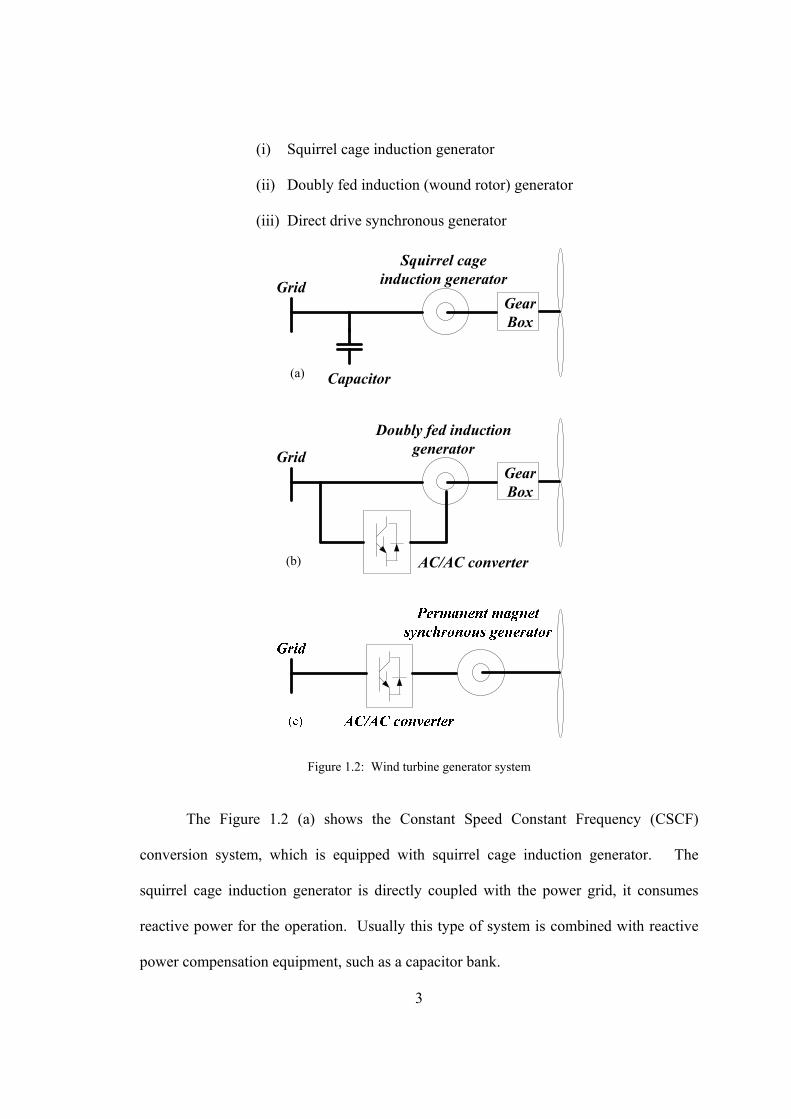
2.3.2.1 Review Induction Machine Principle
This sub-section reviews induction machine principles relevant to Rotor Position
PLL. Derived from (2.13), the equivalent circuit of the induction machine in the -
frame is shown in Figure 2.2. Based on Kirchhoff’s Current Law at the nodes of the
mutual inductance Lm
0
0
r
r
m
m
s
s
i
i
i
i
i
i (2.27)
where
m
m
i
iis the vector of the magnetization currents. The relationship of the vector is,
is', im, ir are shown in figure (2.4)
s'si
r
miri
r s
si
Figure 2.4: Criterion of phase angle lock.
On transforming from the synchronously rotating - frame to the stationary d-q

27
frame, (2.27) becomes
0
0
rq
rd
mq
md
sq
sd
i
i
i
i
i
i (2.28)
In the d-q frame, the currents in (2.28) are at supply frequency S of the stator
voltage. Writing
mq
md
sq
sd
sq
sd
i
i
i
i
i
i'
'
(2.29)
it follows from (2.28) that the rotor currents are:
'
'
sq
sd
rq
rd
i
i
i
i (2.30)
Equation (2.30) describes the requirement that the magnetic flux space vector of
the rotor currents is equal and opposite to the magnetic flux space vector of the stator side
currents together with the magnetization currents.
The rotor currents measured by current sensors are (ir, ir) in the - frame at
angular frequency r. The - frame currents are related to d-q frame currents by
rd rj m
rq r
i ie
i i
(2.31)
where the frame transformation matrix is
cos sin
sin cosm mj m
m m
e
(2.32)
and where m=mt+δm is the angular position of the rotor. The information regarding the
speed m and the angle δm are lost on transforming from the - frame to the d-q frame
and thereafter to the - frame. The objective of the Rotor Position PLL is to recover (m,
δm ).

28
2.3.2.2 Schematic of the Rotor Position PLL
Figure 2.5: Schematic of Rotor Position PLL. Figure 2.5 is the schematic of the Rotor Position PLL. Its measurement inputs
are: 3-phase stator currents, 3-phase rotor currents and 3-phase stator voltages. The a-b-c
quantities are first converted to - quantities. Because of open neutral Y connections of
the stator and the rotor windings, the zero sequences are dropped. The d-q stator currents
(isd, isq) are cosine and sine functions of the argument (st+s) and the - rotor currents
(ir, ir) are cosine and sine functions of the argument (rt+r). The magnetization
currents are not measured directly. They are obtained by making use of the stator
voltages obtained from measurements and dividing them by the magnetization
reactance SmjL . The stator voltages (vsd, vsq) after passing through the 1/(LmS) block
yield the magnetization currents (imd, imq). The stator side currents (iSd, iSq) and (imd, imq)
are summed to form (i’sd, i
’sq) of (2.29).
Figure 2.5 has the traditional “Voltage Controlled Oscillator” (VCO) block and

29
the Detector block of a phase lock loop. The VCO consists of the P-I block and the
integrator 1/s block after the error signal x which is the output of the Detector. The
output of the P-I block is X. A central frequency 0, close to the stator frequency s, is
added and the sum, x, is treated as an algebraic unknown to track the rotor speed m.
After the integrator 1/s block, the argument x=xt+x is formed to track the rotor
position. The variable x is the algebraic unknown to track rotor position. The outputs of
the cos and sin blocks are cos(xt+x) and sin(xt+x). The block ( )[ ]x xj te implements
the transformation of the rotor currents (ir, ir) to
'
'xrd rj
rq r
i ie
i i
(2.33)
Note that X=xt+δX replaces m=mt+δm in (2.31) and (2.32). The Rotor
Position PLL applies (2.33) to replicate the induction machine transformation of (2.31).
At this point, (2.30) is generalized by letting the rotor currents in the d-q frame to
take the time function of the general form
)(
)(
tz
ty
i
i
rq
rd (2.34)
As will be seen later, this step is taken as an easy way to prove that the Rotor
Position PLL is insensitive to measurement noise. From (2.30)
)(
)('
'
tz
ty
i
i
sq
sd (2.35)
Essentially, the measurement noise is on both the stator and the rotor sides
because of the induction process. Substituting (2.34) in (2.31)

30
( )
( )r j m
r
i y te
i z t
(2.36)
Substituting (2.36) in (2.33)
'
'
( )
( )
( )
( )
( )
x m
x m
rd j j
rq
j
i y te e
i z t
y te
z t
(2.37)
where )()( mxmxmx t
When mx and mx ,
)(
)('
'
tz
ty
i
i
rq
rd (2.38)
Equating (2.38) and (2.35), it follows that
'
'
'
'
sq
sd
rq
rd
i
i
i
i (2.39)
The condition in which decoupled P-Q control can be implemented is satisfied
when mx and mx because on back substituting from (2.39), equation (2.13) of
the - frame is satisfied.
2.3.3 Robustness with Respect to Noise and Double PLL
2.3.3.1 Robustness to Noise
The tracking of the rotor speed m and the rotor position δm by the algebraic
unknowns x and δx is accomplished by the VCO which reduces the error x by negative
feedback to zero. The error x is computed by the Detector as:
''''rqsdrdsqx iiii (2.40)
31
On substituting (2.35) and (2.37), the error is
)]()sin[(])()([ 22mxmxx ttzty (2.41)
The error x drives the VCO in negative feedback until the argument in the sine
function is zero. This is when x=m and x=m.
From (2.41), the method is robust because any noise in the current measurements
are in [y(t)2+ z(t)2] and not in the argument of the sine function. This property is a
consequence of the physics of the system because noise on the stator side in (2.35) is
electromagnetically induced in the rotor currents in (2.34).
2.3.3.2 Reduction of Noise by Double PLL
The noise ])()([ 22 tzty in δ is reduced first by the P-I block after x , the output of
the detector, and then by the 1/s integrator block which converts frequency X to
angle X . This requires making the proportional gain Kp small. One reason why Kp
cannot be reduced beyond a certain value without instability is the large frequency range,
-0.30 X 0.30, within which X has to roam. This range is required because the
DFIG operates within 0.3 slip. In order to reduce the range of frequency tracking, the
double PLL design of Figure 2.6 is proposed.
In Figure 2.6, the upper PLL has a fixed center frequency at 60 Hz, i.e. 01=120.
This PLL serves to track the wide range of operating frequency (1-0.3) ×120 X1
(1+0.3) ×120 . The proportional gain Kp1 and the integral gain KI1 are chosen to assure
successful tracking over the extensive frequency range. The output speed X1 of the
upper PLL, after having its fluctuations removed by a low pass filter (LPF), becomes the
center frequency of the lower PLL, i.e. 02 =X1.

32
iSS t irr t
cos sincos sin
{( )
( )}r x
ir x
t
cos sin
xxt
irr t iSS t
)( xxtje
01
a b c
a b c
j se
j se
cos sin
cos sin
iSSt
m s
j
L
1x
Detector
a b c
Si ri
Detector
cos
sin
1
s
iSS t sincos
{( )
( )}r x
ir x
t
2x
DFIG
StatorPLL
P I
P I
LPF
02
1x
2x2x
1x
Figure 2.6: Schematic of double PLL.
With respect to the lower PLL, since its center frequency, 02 =X1, is close to the
objective of tracking, the range of its frequency deviation X2 is small. Therefore, the
proportional gain Kp2 and the integral gain KI2 can be chosen to reduce the noise in X2
and X2 without causing instability. The values used in the simulations are: Kp1=2,
KI1=40, Kp2=0.25, KI2=15.
The simulations of Figure 2.7 show the results of a test of the double PLL
concept. Figure 2.7 shows: (a) the position error position = X - m, where m is obtained

33
from the position encoder of the simulation software; (b) the speed estimate X ; (c) the
stator-side power output SP . Before the step change at 10s shown in Figure 2.7, only a
single PLL is in operation. The double PLL is activated at the step change. One sees
significant reduction in the noise of the position error and the speed by the double PLL.
The imperceptible reduction in noise in the power output in Figure 2.7 (c), during
the significant step reduction of the noise in X , points conclusively to the fact that the
Rotor Position PLL is not a source of noise in the stator power. Note the expanded time
axis. The noise in Figure 2.7 (c) is identifiable as the injected 5th harmonic and IGBT
switching noise.
(a)
(b)
(c)
Figure 2.7: Simulation test on Double PLL (a) Position error position; (b) Speed; (c) Stator-side power.
It is well known that PLLs are good filters of noise. The first stage of filtering is
the P-I block after the detector. But its output is a relatively noisy speed estimate X . The
second stage 1/s integrator block results in very significant reduction. It reduces the 5th
harmonic by 5×60×2 =1884, for instance.

34
As the position estimate X is precise enough and the speed estimate is not critical
to decoupled P-Q control, there is no necessity to apply the double PLL concept. The
noise in the speed estimate can be removed by a traditional filter.
2.3.4 Robustness with respect to Parameters of DFIG
Another robustness feature of the Rotor Position PLL is evident from (2.41). The
error is formed from current measurements. Only the magnetization currents are not
measured. They are estimated from the stator voltages and the magnetization inductance
Lm. No other machine parameters are required for the tracking. As the magnetization
reactance is designed by manufacturers to be as large as possible in induction machines,
the magnetization currents (imd, imq) are small and for this reason high accuracy in
measuring Lm is not required. This is confirmed in experimental results which show that
decoupled P-Q operation is possible over an extensive operating range even when the
magnetization inductance is assumed to be infinite.
2.3.5 Design Considerations
The transfer function kp+kI/s, which lies between the detector error X and the
frequency deviation Δx is a filter of noise from current measurements. Therefore, it is
desirable to keep kp as small as possible. Unfortunately when kp is too small, the window
of frequency acquisition is small. Since the rotor frequency varies between (1.0-0.3)syn
and (1.0+0.3)syn, (for operation with maximum slip of 0.3), kp must be kept reasonably
large. For this reason the speed measurement is noisy as will be seen in the experimental
measurements. The noise in the angle measurement is reduced by the 1/s block. From
(2.41), tracking is not determined by the size of the currents which appear as [y(t)2+

35
z(t)2], but by the frequency and the angle in the argument of the sine function which is
[(x– m)t+(δX – δm )]. Therefore, accuracy is not affected when the power and current
levels are low. The P-I gain constants of Figure 2.5 have been chosen by trial and error
with the help of commercial real-time rapid control prototyping equipment.
2.3.6 Proofs of Speed and Position Tracking by Simulations
Because the laboratory does not have an absolute position encoder to calibrate the
Rotor Position PLL, simulations are applied to fill this gap. Simulation includes the
software models of DFIGs, dc motors, speed and position transducers. Detailed IGBT
switching of the back-to-back VSC under sinusoidal pulse width modulation (SPWM) are
simulated.
2.3.6.1 Response Time of Speed and Position Tracking
In this simulation test, a dc motor drives the DFIG at a constant speed m and its
rotor position m is a ramp. At 400 ms, the designed Rotor Position PLL of Figure 2.5 is
activated.
The dotted lines in Figure 2.8 (a) and (b) are from the software transducers. They
show the machine’s rotor speed (rad/s). The solid lines are from the designed Rotor
Position PLL. After activated, the Rotor Position PLL starts to track the DFIG’s rotor
shaft speed and quickly locks with it. The solid line of the rotor position overlaps the
dotted line but it is deliberately displaced in Figure 2.8 (b) for clarity. The estimated rotor
speed has not been filtered.

36
(a) Transient test of speed estimation
(b) Transient test of position estimation
Figure 2.8: Fast Response of Rotor Position PLL.
2.3.6.2 Insensitivity to Measurement Noise
Based on using the software position transducer as reference, Figure 2.9 shows
that the error of the Rotor Position PLL is around 0.11 degree, an accuracy lying between
an 11- and a 12-bit absolute position encoder. The noise in the current measurement
appears as fluctuation [y(t)2+z(t)2] around the average. In order to show that the Rotor
Position PLL is insensitive to noise, at t=14 seconds the 3-phase ac voltage supply of the
DFIG injects 5th and 7th voltage harmonics, each in the order of 10%. Figure 2.10 shows
that after the transient has damped out, the average, which according to (2.41) is the
estimated position, is unaffected.

37
Figure 2.9: Simulated error of Rotor Position PLL using the software position (transducer as reference)
2.4 Rotor Position PLL for Decoupled P-Q Control of DFIG
Decoupled P-Q control [27-31] enables doubly-fed induction generators to
execute diverse strategies of wind power acquisition, wind power smoothing and ac
voltage support in wind farms. Presently, mechanically mounted position encoders are
needed to implement decoupled P-Q control. The published papers [39-41] have
presented the principles of operation of the Rotor-Position Phase Lock loop, an invention
which can replace mechanically mounted position encoders with minimal cost.
2.4.1 Implementation of Decoupled P-Q control of DFIG
Figure 2.3 shows the grid-side VSC and the rotor-side VSC in back-to-back rotor-
side control of the DFIG. The grid-side VSC conveys the slip power automatically to the
60 Hz ac grid by using its active power control to maintain the voltage across the dc
capacitors. Also the grid side VSC has the ability to regulate the power factor at AC side.
A 3-phase transformer matches the high grid-side voltage to the low voltage of the VSCs.

38
Figure 2.10: Block diagram of rotor side VSC control of DFIG.
Figure 2.10 shows the rotor-side control which implements the decoupled P-Q
control. The commands are taken from the PS, QS Reference Generator which issues the
references PS*, QS
*. The stator current references iS*=PS*/vS and iS*=QS
*/vS are
converted to rotor current references ir* and ir* through (2.26). Since true control is by
the rotor voltages (vra, vrb and vrc), the rotor current references are produced by negative
feedback. The rotor currents (ira, irb and irc) are measured, transformed to the - frame as
(ir , ir ) and P-I gains ensure that (ir*, ir* ) are tracked by negative feedback. Trial and
error with real-time, rapid control prototyping equipment has been used to select the
proportional and integral gain constants to ensure fast and stable operation. The
transformations to and from - and d-q frames are by the ][ Sje transformation blocks
which make use of S, the phase angle of the stator voltage from the Stator Voltage PLL.
The transformations to and from d-q and - frames are by the ][ xje transformation
blocks which make use of x = δr, the estimate of the position of the rotor winding axis
which come from the Rotor Position PLL.
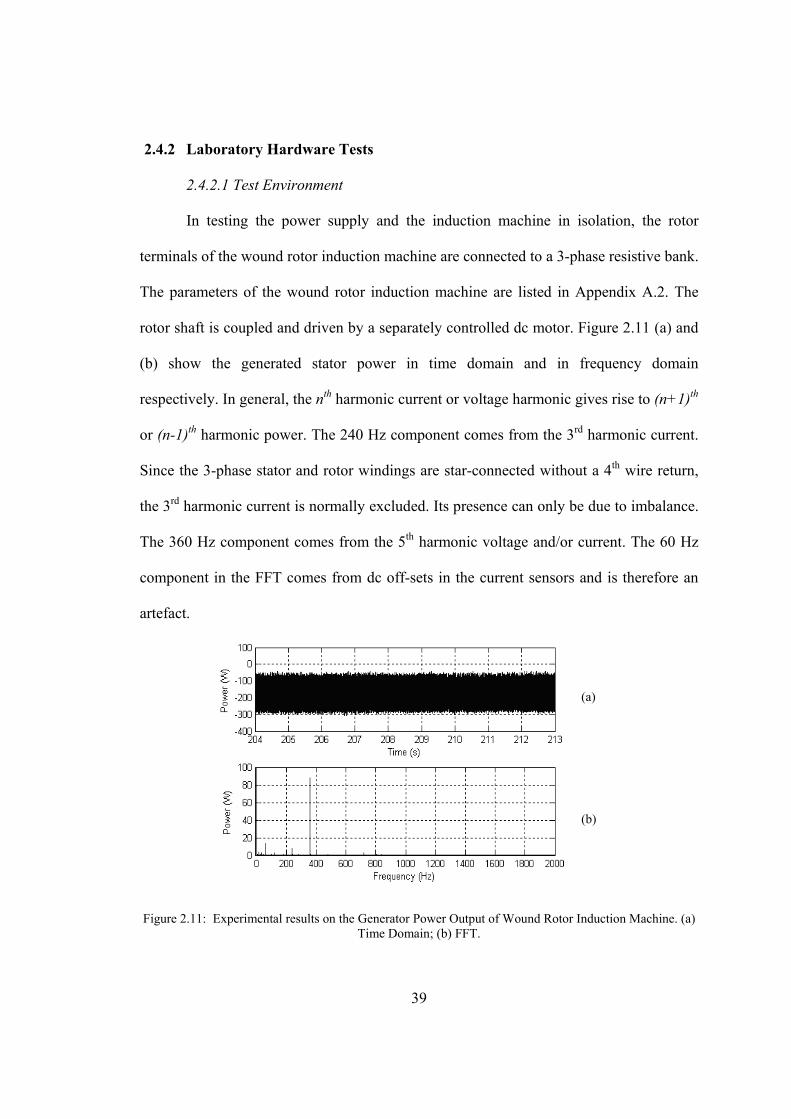
39
2.4.2 Laboratory Hardware Tests
2.4.2.1 Test Environment
In testing the power supply and the induction machine in isolation, the rotor
terminals of the wound rotor induction machine are connected to a 3-phase resistive bank.
The parameters of the wound rotor induction machine are listed in Appendix A.2. The
rotor shaft is coupled and driven by a separately controlled dc motor. Figure 2.11 (a) and
(b) show the generated stator power in time domain and in frequency domain
respectively. In general, the nth harmonic current or voltage harmonic gives rise to (n+1)th
or (n-1)th harmonic power. The 240 Hz component comes from the 3rd harmonic current.
Since the 3-phase stator and rotor windings are star-connected without a 4th wire return,
the 3rd harmonic current is normally excluded. Its presence can only be due to imbalance.
The 360 Hz component comes from the 5th harmonic voltage and/or current. The 60 Hz
component in the FFT comes from dc off-sets in the current sensors and is therefore an
artefact.
(a)
(b)
Figure 2.11: Experimental results on the Generator Power Output of Wound Rotor Induction Machine. (a) Time Domain; (b) FFT.

40
2.4.2.2 Static Test of Prototype
The prototype operates under decoupled P-Q control with the Rotor-Position PLL.
Fig. 2.12 shows a sample of the steady-state stator power output in (a), with its FFT in
(b). In Figure 2.12 (b), a 120 Hz component, which must have come from unbalance in
the power electronics system, is added to the 60, 240 and 360 Hz components of Figure
2.11 (b). The IGBT switching noise appears at 1480 Hz.
(a)
(b)
Figure 2.12: Experimental results on Stator Power Output of the Prototype under Decoupled P-Q Control with Rotor-Position PLL (a) Time Domain; (b) FFT.
Figure 2.13 shows the quality of the 3-phase rotor currents in (a) and the 3-phase
stator currents in (b). By comparing the time domain waveforms of Figure 2.13 with
those of Figure 2.11 and 2.12, the poor appearance of the power waveforms is related to
the compressed time scale.
Figure 2.14 shows the FFTs of the waveforms of one current phase of Figure
2.13. The dominant frequency of the stator current is 60 Hz and its slip frequency on the
rotor side is 2.4 Hz. The FFT of the stator current shows the 120 Hz (2nd harmonic) from
unbalance, the 180 Hz (3rd harmonic) and the 300 Hz (5th harmonic) from magnetic

41
saturation. From Section 2.3.3, one concludes that the noise of the prototype originates
from IGBT switching, slight unbalance in the 3-phases, 3rd and 5th harmonics of
ferromagnetic saturation
(a)
(b)
Figure 2.13: Experimental three phase current waveforms. (a) rotor (2.4 Hz); (b) stator (60 Hz).
(a)
(b)
Figure 2.14: FFT of experimental current waveforms. (a) rotor (signal-2.4 Hz); (b) stator (signal-60 Hz).

42
2.4.2.3 Dynamic Tests of Prototype
Figure 2.15 shows the stator complex power PS and QS of the prototype in
response to step changes in the references, Pref and Qref. The experiment has been planned
to demonstrate the decoupling of the P and the Q control over a wide operating range. In
a step change of Pref for instance, QS is disturbed only briefly. The converse applies. As
Figure 2.11 has recorded, the noise in PS and QS are due to noise from slight unbalance
and magnetic saturation.
60 70 80 90 100 110 120 130 140 150-3500
-3000
-2500
-2000
-1500
-1000
-500
0
500
1000
Time (s)
P a
nd Q
(W
& V
ar)
Ps
PrefQs
Qref
Figure 2.15: Experimental results on responses to step changes in stator references Pref and Qref.
35.4 35.6 35.8 36 36.2 36.4 36.6-3000
-2500
-2000
-1500
-1000
Time (s)
P (
W)
Ps
Pref
45.6 45.8 46 46.2 46.4 46.6-1500
-1000
-500
0
500
Time (s)
Q (
Var
)
Qs
Qref
(a)
(b)
Figure 2.16: Experimental results on Complex Power Step Response. (a) Real Power; (b) Reactive Power.

43
Figure 2.16 (a) shows, on an expanded time scale, the speed of response of PS due
to a step change in the reference. The response of QS is not recorded. Figure 2.16 (b)
shows the speed of response of QS due to a step change of its reference in an entirely
separate experiment. The settling time of PS is within 0.26s and that of QS is within
0.36s. As the wind-turbine blades have moments of inertia with time constants of H=4s,
no effort has been made to shorten the time of response further.
In wind farm operation, PS of the DFIG is expected to track a reference Pref
determined by a control strategy of the operator. Figure 2.17 demonstrates this capability
in the generated power range from 1 kW to 3 kW, the latter being 80% of the rating of the
induction machine. As the power to implement this experiment comes from the dc
chopper driven dc motor, a higher power rating and a higher oscillating frequency are not
within the reach of our laboratory.
In the same experiment in which Figure 2.17 was recorded, the estimate of rotor
speed x m was also recorded and it is shown as Figure 2.18. The synchronous speed
of 1800 rpm is shown in Figure 2.18 to bring home the point that the power of Figure
2.17 is generated partly at sub-synchronous speed and partly at super-synchronous speed.
The noise in x comes from the noise in the stator and rotor currents. Unlike the rotor
position, the rotor speed is not essential in the implementation of decoupled P-Q control.
In many control strategies, such as MPPT operation which will be explained in Section
2.5, rotor speed is used only as a pointer to the Look-Up Tables in the Pref (m) and Qref
(m) references. A low pass filter can remove the noise without affecting control stability,
as has been verified experimentally.

44
Figure 2.17: Experimental results on tracking capability of PS.
Figure 2.18: Experimental results on estimate of rotor speed x m.
2.4.2.4 Tests on Sensitivity of Parameter Variations
The operation of the Rotor-Position PLL does not require knowledge of the
resistance and the leakage inductance of the stator and the rotor of the DFIG. The only
parameter required is the magnetization inductance. In fact, when the operating stator and
rotor currents are large compared to the magnetization current, one can assume Lmωs→
∞.
Figure 2.19 displays experimental results in tests similar to Figure 2.15 but with
the difference that the magnetization reactance of 39.6 ohm, taken from Appendix A.2,
has been replaced by Lmωs=∞. Figure 2.19 demonstrates the high insensitiveness to
variation in the magnetization reactance. But instability sets in at low rating operation
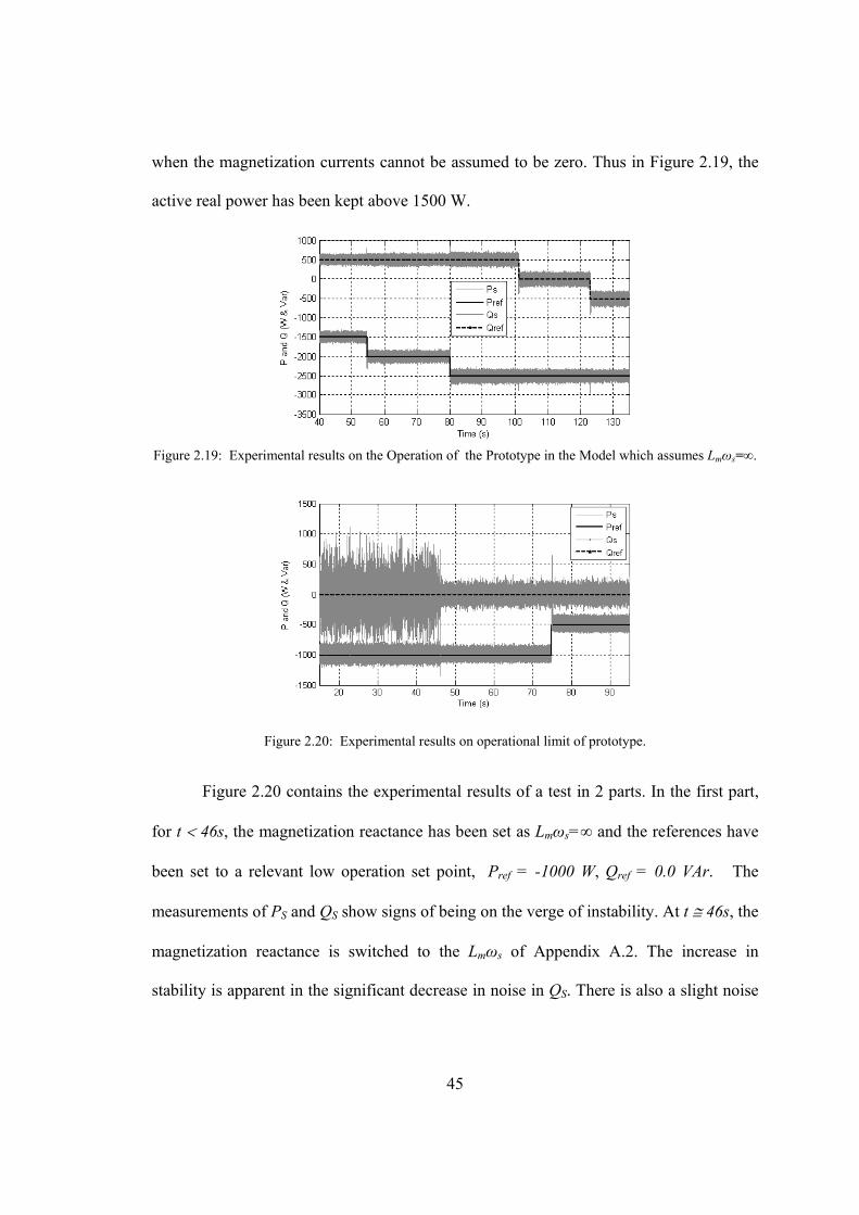
45
when the magnetization currents cannot be assumed to be zero. Thus in Figure 2.19, the
active real power has been kept above 1500 W.
Figure 2.19: Experimental results on the Operation of the Prototype in the Model which assumes Lmωs=∞.
Figure 2.20: Experimental results on operational limit of prototype.
Figure 2.20 contains the experimental results of a test in 2 parts. In the first part,
for t 46s, the magnetization reactance has been set as Lmωs=∞ and the references have
been set to a relevant low operation set point, Pref = -1000 W, Qref = 0.0 VAr. The
measurements of PS and QS show signs of being on the verge of instability. At t 46s, the
magnetization reactance is switched to the Lmωs of Appendix A.2. The increase in
stability is apparent in the significant decrease in noise in QS. There is also a slight noise

46
decrease in PS. At t 74s, the active power reference is decreased to Pref = -500 W and
the prototype responds without being unstable.
The experiments of Figure 2.19 and 2.20 demonstrate that although the Rotor
Position PLL requires knowledge of the magnetization reactance, its accuracy is not
critical.
2.4.2.5 Tests on Synchronous Speed
Tests have shown that the Rotor Position PLL has a full range of speed operation,
from negative speed to super-synchronous speeds. Figure 2.21 shows operation at
synchronous speed syn at which the experimental rotor current irc is held virtually as a dc
current for 10 seconds (longer if required). The slight variations in ira and irb come from a
slow drift in δm. In this experiment, the VCO of the Rotor Position PLL outputs x=syn
so that the rotor frequency r=0.
138 139 140 141 142 143 144 145 146 147 148-20
-15
-10
-5
0
5
10
15
20
Time (s)
Rot
or c
urre
nt (
A)
irb
ira
irc
Figure 2.21: Experimental rotor phase currents at synchronous speed.
Experimental tests have demonstrated that the Rotor Position PLL enables
decoupled P-Q control of a prototype DFIG to be implemented. The Rotor Position PLL
is robust because the magnetization reactance of the DFIG is the only information
required for it to operate in the full range. In the range where the operating line currents

47
are large compared to the magnetization current, the magnetization reactance can be
assumed to be infinite.
The Rotor Position PLL has passed tests in an environment containing harmonics
arising from unbalance and saturation of iron. An analysis has been presented explaining
why it is insensitive to noise. A further simulation test has been presented to show that it
does not propagate the noise of the environment.
2.5 Sensorless Maximum Power Point Tracking of Wind by DFIG using
Rotor Position PLL
When no anemometer is used in maximum power point tracking (MPPT) of wind,
the method currently qualifies as sensorless [12-15]. A more demanding definition of
sensorless MPPT would require that not only anemometers but tachometers and absolute
position encoders are not be used. The first stage of “true” sensorless MPPT of wind
power by doubly-fed induction generator has consisted of mastering rotor-side control
using back-to-back VSCs [16-26]. The second stage consists of replacing the absolute
position encoder required for decoupled P-Q control by a sensorless means [27-38]. As
in [13, 14], the implementation of MPPT is also physics based (Newton’s Law of
Motion) and this is in contrast with the research which make use sophisticated
mathematical tools [12, 15, 22].
2.5.1 Introduction of Wind Energy
A wind turbine obtains its power input by converting the force of the wind into
torque acting on the rotor blades. The amount of energy which the wind transfers to the
rotor depends on the density of the air, the rotor area, and the wind speed. The energy

48
content of the wind varies with the cube of the average wind speed. The power of the
wind passing perpendicularly through a circular area is given as:
3 21
2Wind air wP v r (2.42)
where WindP = the power of the wind (W )
air = the density of dry air ( 225.1 3mkg )
wv = the velocity of the wind ( sm )
r = the radius of the turbine ( m )
The wind speed is always fluctuating, and thus the energy content of the wind is
always changing. Energy output from a wind turbine will vary as the wind varies,
although the most rapid variations will to some extent be compensated for by the inertia
of the wind turbine rotor.
Betz' law states that one can only convert less than 16/27 (or 59%) of the kinetic
energy in the wind to mechanical energy using a wind turbine. The actual amount of
power capable of being produced by a wind turbine is given by:
3 21( )
2Wind air w pP v r C (2.43)
where )(pC is the power coefficient of the wind turbine
pC is dependent on the ratio between the tangential velocity of the blade tip and
the wind velocity. This ratio λ known as the tip-speed ratio, is defined as:
_m rgear ratio
v
(2.44)
where m = the angular velocity of the generator ( srad / )

49
The power coefficient of a wind turbine (both for fixed and variable pitch), pC , is
optimized for the most probable local wind speed. This is a deliberate choice by the
engineers who designed the turbine. At low wind speeds efficiency is not so important,
because there is not much energy to harvest. At high wind speeds the turbine must waste
any excess energy above what the generator was designed for. Efficiency therefore
matters most in the region of wind speeds where most of the energy is to be found.
2.5.2 Principle of MPPT
It is now widely known how, from a Cp-vs- curve [5, 6], the family of wind
power PW-vs-m curves such as those of Figure 2.22 can be drawn.
Figure 2.22: Wind power PW as function of generator speed m for different wind velocities vW.
Figure 2.22 has been synthesized from the data of Figure 24.2 (b) on page 530 of
[6]. MPPT is implemented by loading the generator power PG so that the wind turbine
follows the hatched line, PG–vs-m, which passes through all the peaks. This curve
correspond to one point (Cpopt, opt ) of the Cp-vs- curve.
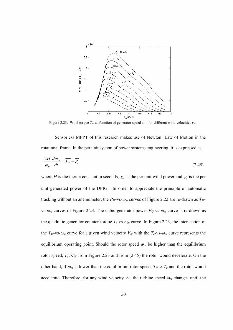
50
Figure 2.23: Wind torque TW as function of generator speed m for different wind velocities vW .
Sensorless MPPT of this research makes use of Newton’ Law of Motion in the
rotational frame. In the per unit system of power systems engineering, it is expressed as:
eWm PP
dt
dH
0
2
(2.45)
where H is the inertia constant in seconds, WP is the per unit wind power and
eP is the per
unit generated power of the DFIG. In order to appreciate the principle of automatic
tracking without an anemometer, the PW-vs-m curves of Figure 2.22 are re-drawn as TW-
vs-m curves of Figure 2.23. The cubic generator power PG-vs-m curve is re-drawn as
the quadratic generator counter-torque Te-vs-m curve. In Figure 2.23, the intersection of
the TW-vs-m curve for a given wind velocity VW with the Te-vs-m curve represents the
equilibrium operating point. Should the rotor speed m be higher than the equilibrium
rotor speed, Te TW from Figure 2.23 and from (2.45) the rotor would decelerate. On the
other hand, if m is lower than the equilibrium rotor speed, TW Te and the rotor would
accelerate. Therefore, for any wind velocity vW, the turbine speed m changes until the

51
wind torque TW finds an equilibrium with the optimum counter-torque Te which is
controlled by the PS, QS Reference Generator block in Figure 2.10. Since all the
intersection points lie on the right-hand side of the peak wind torques in the family of
wind velocity curves, the equilibrium points are all stable. Because the wind velocity
fluctuates, the rotor speed keeps changing to track the optimum power of the wind
velocity.
2.5.3 Designing Ps* Reference
Recall the information introduced in Section 2.2.4. PS*, in the Reference
Generator block in Figure 2.10, controls the stator power. Neglecting ohmic losses, the
stator power is, from induction machine theory, the airgap power
syneS TP (2.15)
where Te is the induction machine torque output and syn is the synchronous speed of the
grid frequency. The electromechanical output power of the induction machine is:
mee TP (2.16)
Pe is the algebraic sum of the stator power and the rotor power, passes through the
rotor slip rings and the grid-side VSC. For MPPT, one designs Pe so that it follows PG –
vs-m curve of Figure 2.22. PG can be equated as:
mgG kP 3 (2.46)
where kg is a proportionality constant. Equating Pe=PG and eliminating Te by substituting
(2.15), the Power Reference in Figure 2.10 must compute
2*msyngSref kPP (2.47)
The speed m is obtained from the Rotor Position PLL.

52
2.5.4 Proof of Sensorless MPPT by Simulation
A 600-second wind velocity file is used to conduct the simulation test with the
configuration shown as Figure 2.24. The average wind velocity is 12 m/s and the WTG
has an inertia constant of H=4 second.
m
curve
Cp
Wv
WindPrefP refQ
Figure 2.24: Rotor side control of DFIG by back-to back voltage source converters (VSCs)
Figure 2.25 (a) displays a sample of the simulated wind power PWind and
generated power Pe. Figure 2.25 (b) shows the rotor speed m (per unit) which
accelerates when PWind Pe, and decelerates when PWind Pe. The rotor speed m carries
the power reference Pref=kgsynm2
with it. As proof of successful MPPT, the value of
Cp(t) is computed from the simulated values of m(t) and PW(t) for fluctuating wind
velocity vW(t). Figure 2.25 (c) shows Cp(t) fluctuating slightly below the optimum value
of Cpopt=0.53. (The quoted value is the mechanical power efficiency coefficient. As
pointed out by [6], when mechanical losses are deducted, Cpopt takes a value which is
usually lower than 0.5.) The slight inaccuracy (about 2%) is related to the fact that Figure
2.23 has a family of flat maxima so that there is uncertainty in determining the constant

53
kg of (2.46). Nevertheless, the simulation is sufficient to validate the claim that MPPT is
achieved without an anemometer. As the Rotor Position PLL replaces the mechanical
tachometer and absolute position encoder, the MPPT is sensorless in the demanding
definition.
Figure 2.25: Simulation of (a) PW wind power, Pe DFIG electrical power; (b) DFIG speed; (c) Cp(t)-- MPPT strategy .

54
Chapter 3: Standalone Doubly-Fed Induction Generators with
Autonomous Frequency Control
3.1 Introduction
Because most wind-turbine generators in the 1.5 to 3.5 MW range are coupled to
doubly-fed induction generators [60], DFIGs continue to be researched. Sophistication,
such as decoupled P-Q control, has been built on to DFIGs [34-40]. Through
controllability over active power P, the wind turbine generator readily implements
maximum power point tracking (MPPT) which increases the yield significantly. Through
controllability over reactive power Q, low voltage ride through (LVRT) strategies are
easily implemented.
Decoupled P-Q control requires hardware and software in making reference frame
transformations (a-b-c, -, d-q, -). The stator phase lock loop is used to acquire the -
frame voltages and the information to transform to the - frame. A rotor position
sensor is used to locate the instantaneous positions of the rotor winding axes. Rotor
position sensors are mostly mechanical incremental position encoders. The challenge to
do without mechanical sensors has yielded several publications on sensorless DFIGs [30-
41]. As incremental position encoders have been known to be faulty [7], adding
sensorless method to position encoders would increase reliability.
As the normal operation of DFIGs has, by and large, been addressed, research has
turned to their ability to handle fault conditions. One major problem is when a wind farm
is islanded. When a wind farm is islanded, the DFIGs are deprived of the utility grid

55
frequency as reference. Even before the advances of power electronics, standalone
operation of induction generators is possible [42]. Recent research [43-52] which
incorporates power electronic control, brings the standalone DFIGs nearer to islanded
wind farm operation. To date, the advances on islanded renewable energy sources are
restricted to systems whose voltage-source converters (VSCs) (front end of frequency
changers) feed directly to the point of common coupling (PCC) [53-59]. But the
controlling VSC of a DFIG feeds the rotor slip rings.
This thesis continues the advances on standalone DFIG research by showing that:
(1) generate autonomous ac voltages with controllable frequency;
(2) synchronize with other standalone DFIGs to form a common islanded
wind farm grid frequency; The farm frequency originating from multiple
DFIGs ensures greater reliability because the entire wind farm grid would
disintegrate if the island frequency depends on a single Master frequency
and the Master is lost.
(3) use the islanded wind farm grid frequency to communicate the status
power delivery for load sharing without telecommunication channels.
(4) make a seamless transition from pre- to post-islanding status;
(5) ensure that Wind Turbine Generators do not accelerate beyond the safe
rotor speed limit because the wind farm has excess of wind power when
suddenly cutoff from the grid load.

56
The autonomous voltage generation is produced by feedback.
Understanding the feedback method requires studying the phase angle of the
generated frequency in two portions of the feedback loop:
(i) through the DFIG and its decoupled P-Q control, as described in
Chapter 2,
(ii) through the stator PLL.
This chapter will show in detail how the frequency is controlled by the references
of the decoupled P-Q control and how multiple DFIGs mutually synchronize. The chapter
also presents the theoretical foundations which explain:
(i) how the reference settings of the power control affects the autonomous
frequency; and
(ii) how the autonomous frequencies of DFIGs in an islanded wind farm
synchronize to a common grid frequency.
It needs to be pointed out that the method of (ii) is not the same as DFIGs
synchronizing to a single frequency set by the utility grid (50 or 60 Hz) or by a Master
frequency source in the wind farm. The frequencies mutually converge to a weighted
average of the initial frequencies of the autonomous DFIGs.
3.2 Self-Sustained Induced Stator Voltages in DFIG
3.2.1 Operating Principles
Before islanding, the stator PLL of each DFIG, as explained in chapter 2, is
locked to the frequency ω0 of the utility grid. Under decoupled P-Q control, each DFIG
produces an ac voltage at the stator terminal which is also at grid frequency ω0. This
stator ac voltage originates from the dc voltage of the capacitor between the back-to-back

57
VSCs. The decoupled P-Q control, commands the rotor-side inverter to produce ac
voltages at rotor slip frequency ωr. (To avoid bookkeeping of pole-pairs, rotor angles are
given in electrical radians.) The rotor ac voltages feed the slip rings of the wound rotor
induction machine and produce a magnetic field which rotates at angular velocity of ωr
with respect to the rotor iron. As the rotor iron turns at angular velocity of ωm, the
magnetic field is carried along with it so that the resultant airgap magnetic field has the
angular velocity of ωr+ωm=ω0 and induces stator voltages at frequency ωr+ωm=ω0 , as
back emf to the utility grid voltage.
When the utility grid is lost, momentarily the stator voltage has a frequency ωS
which, in general is different from ω0. Through the same decoupled P-Q control which
produces voltage at ωr+ωm=ω0 when the grid is connected, the standalone DFIG produces
voltages at frequency ωr+ωm=ωS at the stator terminal. The DFIG continues generating
this voltage if the feedback condition for self-sustaining is satisfied.
In the initial standalone state, it is assumed that the a-phase voltage, for example,
has momentarily a voltage of the form:
( ) cosa S Sv t V t (3.1)
and the stator PLL measures the phase angle ωSt. From ωSt measured by the PLL, the
stator windings, generate stator voltages whose a-phase is of the form
1 1( ) cos( )a S Sv t V t (3.2)
The angle in (3.2) is formed by time delays along the feedback path of the
signal ωSt as it passes through the control of Figure 3.1 and the rotor and stator windings.
Depending on the positive or negative polarity of Δθ, the frequency ωS keeps increasing
or decreasing. The frequency is constant when Δθ=0, and the voltage with frequency ωS

58
is sustained. In the feedback loop, the “open loop” input signal is the argument of (3.1)
and the “open loop” output signal is the argument of (3.2). The stator-side PLL
completes the closed loop feedback path. In closed loop feedback relating VS of (3.1) and
V1S of (3.2), there is a phase difference Δθ.
The control blocks of the Decoupled P-Q Control of Figure 3.1 hold the reasons
for a part of the delays of Δθ. Figure 3.1 is reproduced from equation (2.10) except for
the “Standalone Operation” block which is added in this chapter. To avoid delving into
the complications in Figure 3.1, for the purpose of this chapter it is sufficient to focus on
how the input phase angle ωSt of (3.1) is changed to the output phase angle (ωSt+Δθ) of
(3.2) as the feedback signal passes through the controls of Figure 3.1 to the rotor-side
VSC and to the DFIG.
r abci
r abcv
ri
ri*ri
*ri
*rv*rv
*si
*si
1
m
s
SP SQ*
refP *refQ
1
m sL
* *ref refP Q Ref.
Generators s
Measured
P and Q
sV
sV
sf
refV*
sP *sQ
sje
f
s
V
1
abc
abc
s abcv
reff
m
mje sje
mje
Figure 3.1: Block diagram of rotor side VSC control of DFIG.
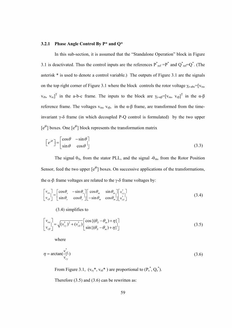
59
3.2.1 Phase Angle Control By P* and Q*
In this sub-section, it is assumed that the “Standalone Operation” block in Figure
3.1 is deactivated. Thus the control inputs are the references P*ref =P* and Q*
ref=Q*. (The
asterisk * is used to denote a control variable.) The outputs of Figure 3.1 are the signals
on the top right corner of Figure 3.1 where the block controls the rotor voltage vr-abc=[vra,
vrb, vrc]T in the a-b-c frame. The inputs to the block are vr-αβ=[vrα, vrβ]
T in the α-β
reference frame. The voltages vrα, vrβ, in the α-β frame, are transformed from the time-
invariant γ-δ frame (in which decoupled P-Q control is formulated) by the two upper
[ej] boxes. One [ej] block represents the transformation matrix
cos sin
sin cosje
(3.3)
The signal S, from the stator PLL, and the signal -m, from the Rotor Position
Sensor, feed the two upper [ej] boxes. On successive applications of the transformations,
the - frame voltages are related to the - frame voltages by:
*
*
cos sin cos sin
sin cos sin cosr s s m m r
r s s m m r
v v
v v
(3.4)
(3.4) simplifies to
* 2 * cos{( ) }( ) ( )
sin{( ) }r S m
r rr S m
vv v
v
(3.5)
where
*
*arctan( )r
r
v
v
(3.6)
From Figure 3.1, (vr*, vr* ) are proportional to (Ps*, Qs
*).
Therefore (3.5) and (3.6) can be rewritten as:

60
*2 *2 cos( )
sin( )r S m
prop s sr S m
vk P Q
v
(3.7)
where kprop is from the proportionality constants and
*
*arctan( )s
s
Q
P (3.8)
From [vr, vr ]T in (3.7), the block in top right corner of Figure 3.1 sends signals
to the rotor-side VSC to produce the rotor voltages [vra, vrb, vrc]T. The rotor currents [ira,
irb, irc]T which flow produce the rotor magnetic flux. In (3.4), S=St and, in general,
m=mt+m where m is the rotor angle at t=0. The matrix multiplication in (3.4) yields
cosine and sine functions whose are arguments are (St)-(mt+m)+η. Consequently, the
rotor flux rotates at angular velocity r=S-m with respect to the rotor iron. The rotor
iron rotates at angular velocity m. Therefore, the airgap flux rotates at r+m=(S-
m)+m=S with respect to the stator windings and induces the stator voltage of (3.2).
The phase angle is:
s m (3.9)
where ζ is to account for any additional time delay in producing the induced stator
voltage of (3.2).
The angle -m+ζ is a property of the DFIG and the rotor-side VSC. Autonomous
frequency control is possible because P* and/or Q* can be applied in (3.8) to control η
so that Δθ in (3.9) can take different polarity signs:
0; 0; 0 (3.10)

61
When S=-m+ζ0.0, the frequency ωS keeps increasing and vice versa. As S
is measured by the stator phase lock loop, the next section examines the effect of the
different polarities of S on the frequency output of the PLL.
3.3 Phase Lock Loop
3.3.1 Review of PLL Fundamentals
Phase Lock Loops originate from communication engineering [64]. Although
there is active research to increase the robustness, discrimination and speed of response in
a PLL [65], the PLL shown in Figure 3.2 is adequate to display its self-tracking property.
The function of the PLL in Figure 3.2 is to make the output angle track the
input angle S which is the argument of the input voltages [V, V]T=[Vscoss, Vssins]
T.
Detection consists of multiplying the input voltages by sin and cos, to produce the
error = -Vsin+Vcos= -Vssin(-s) for negative feedback tracking. When sin(-
s) is small, approaches (-s). The error passes through a P-I block with proportional
gain Kp and integral gain Ki. The output of the P-I block has the status of angular
frequency ωv. After passing an integrator, the signal becomes .
The operation of the PLL can be understood by first assuming the s. Since
sin(-s)0.0 for –π(-s)0, the error -Vssin(-s) is positive. On passing through
the P-I block and another integration block, keeps increasing because the error is
positive. stops increasing when the error becomes zero. When =s, the tracking is
successful.
The variable before the final integration block in Figure 3.2 is , the frequency
of the PLL. As the PLL is intended to acquire the phase angle of 60 Hz voltages,

62
acquisition is improved by adding a constant frequency c=260 close to the input
frequency. But the PLL functions even when c=0.0.
V
V
c
sin
cos
Figure 3.2: Schematic of 3-phase PLL 3.3.2 Analysis of PLL
Differentiating the output of the PLL
d
dt
(3.11)
On the left side of the integrator of Figure 3.2,
sin( )p s s CK V (3.12)
From the integral of the KI block
sin( )i s s
dK V
dt (3.13)
Substituting (3.12) in (3.11)
sin( )p s s C
dK V
dt
(3.14)
It is necessary to show that converges to S by solving the differential
equations of (3.13) and (3.14) simultaneously.

63
3.3.3 A Closed Form Solution
Because of the nonlinear term sin(s-) in (3.13) and (3.14), there is no analytical
solution. However, it is possible to show analytically that when S0.0, the frequency
ωS keeps increasing with time and conversely when S0.0 the frequency ωS keeps
decreasing with time. When the desired frequency is reached, S should be set to zero.
This controllability comes from changing by PS* and QS
* in (3.8) so as to affect the
polarity sign of S=-m+ζ in (3.9).
Assuming that for t 0, prior to losing the utility frequency, the PLL has been in
synchronism, that is =0 in Figure 3.2. It is assumed that C=0. Since the PLL has been
tracking the grid frequency, =0, and the grid phase angle, =S. Thus from (3.12),
(0)=0.0.
At t=0, as measured by the PLL, =S. At t=0+, immediately after the DFIG is
islanded, the PLL measures the argument of (3.2).
S (3.15)
Because of (3.15), sin(s-) in (3.13) and (3.14),becomes sinΔθν. When ν is
assumed to be constant, on integrating (3.13)
1sin( )i sK V t C (3.16)
Because at t=0, =0 , the constant of integration in (3.16) is C1=0.0. On
substituting (3.16) in (3.14), on integrating
2
2
0.5 sin( ) sin( )i s p s
C
K V t K V t
t C
(3.17)
where C2 is another constant of integration.
As the interest is focused on the frequency, differentiating (3.17)

64
sin( ) sin( )i s P s CK V t K V (3.18)
Thus the frequency of the PLL keeps increasing, keeps decreasing or remains
constant by making sin() positive, negative or zero.
Although the result from (3.18) is useful enough, it depends on the initial
conditions. The graphical method presented in the next sub-section is more general.
3.3.4 Graphical Approach
Since the system equations of (3.13) and (3.14) are two-dimensional ( ,), they
are amenable to two-dimensional graphical (phase-plane) solution [66] which gives a
more comprehensive picture of the system dynamics than the solution of (3.18). In
solving the differential equations (3.13) and (3.14) simultaneously, it is possible to
proceed from state ( (t), (t) ) at time t to the state ( (t+h), (t+h) ) in time t+h
because there are time gradients given by (3.13) and (3.14). Computing the trajectory
from the time gradients is accomplished by using a numerical integration subroutine (for
example, the Runge-Kutta method).
Every point in the phase-plane graph (see Figure 3.3) is a possible state ( (t),
(t) ) of (3.13) and (3.14). The state ( (t+h), (t+h) ) at a later time t+h, is a
contiguous point in the same phase-plane. The two contiguous states are joined to each
other by the gradient d /d. This gradient is obtained by dividing (3.13) by (3.14),
which is:
sin( )
sin( )i s
p s
K Vd
d K V
(3.19)
In (3.19), C in (3.14) is set to zero. This is because the PLL tracks even when
C=0.0. As already explained, C is added to improve the speed of acquisition.

65
(
rad/
s)
0 500 1,000 1,500
300
320
340
360
380
400
420
440
(rad)
(a) > 0.0
(ra
d/s)
(rad)
(b) = 0.0
(ra
d/s)
0 500 1,000 1,500
300
320
340
360
380
400
420
440
(rad)
(c) < 0.0 Figure 3.3: Phase-plane with different
The y- and x-axis in Figure 3.3 are drawn to represent and . Figure 3.3 (a),
(b) and (c) respectively show the gradients of (3.19) of all sample points when 0.0,
= 0.0 and 0.0. An arrow-head is attached to each gradient line to indicate the
direction of the trajectory. Based on (3.14), wherever +KpVSsin(S-) 0 the arrow
head points to increasing values of and vice versa. In using the phase-plane graphs, one
begins at any point (initial value) and follows the trajectory indicated by the arrows.
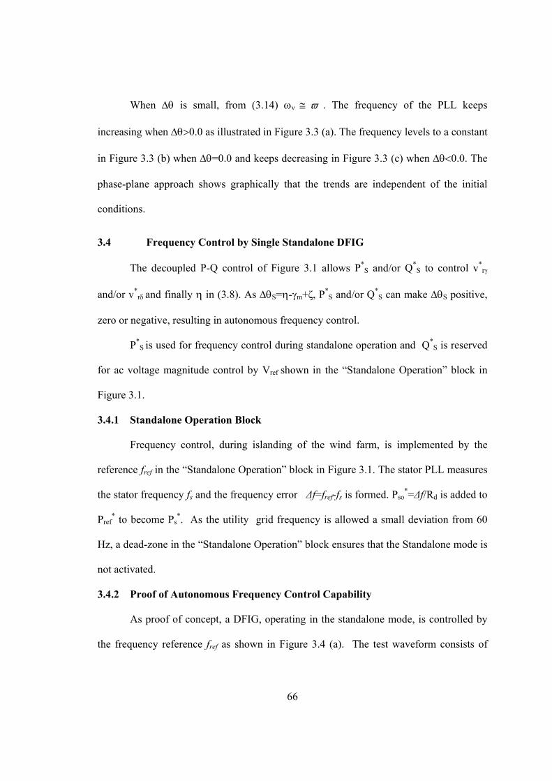
66
When is small, from (3.14) . The frequency of the PLL keeps
increasing when 0.0 as illustrated in Figure 3.3 (a). The frequency levels to a constant
in Figure 3.3 (b) when =0.0 and keeps decreasing in Figure 3.3 (c) when 0.0. The
phase-plane approach shows graphically that the trends are independent of the initial
conditions.
3.4 Frequency Control by Single Standalone DFIG
The decoupled P-Q control of Figure 3.1 allows P*S and/or Q*
S to control v*r
and/or v*r and finally in (3.8). As S=-m+ζ, P*
S and/or Q*S can make S positive,
zero or negative, resulting in autonomous frequency control.
P*S is used for frequency control during standalone operation and Q*
S is reserved
for ac voltage magnitude control by Vref shown in the “Standalone Operation” block in
Figure 3.1.
3.4.1 Standalone Operation Block
Frequency control, during islanding of the wind farm, is implemented by the
reference fref in the “Standalone Operation” block in Figure 3.1. The stator PLL measures
the stator frequency fs and the frequency error Δf=fref-fs is formed. Pso*=Δf/Rd is added to
Pref* to become Ps
*. As the utility grid frequency is allowed a small deviation from 60
Hz, a dead-zone in the “Standalone Operation” block ensures that the Standalone mode is
not activated.
3.4.2 Proof of Autonomous Frequency Control Capability
As proof of concept, a DFIG, operating in the standalone mode, is controlled by
the frequency reference fref as shown in Figure 3.4 (a). The test waveform consists of

67
ramps, sinusoidal variations, step changes to different constant values. The frequency of
the stator voltage follows the reference as the simulated result in Figure 3.4 (b) shows.
5658606264
f ref (
Hz)
3 4 5 6 7 8 95658606264
Time (s)
f s (H
z)
(a)
(b)
Figure 3.4: Simulation Showing Autonomous Control of Frequency
Reference test signal fref-vs-t ; (b) PLL mesurement fS-vs-t.
3.4.3 Proof of Capability to Sustain Islanding Disconnection
Before islanding, the DFIG delivers wind power to the local load and to the utility
grid. On islanding, the DFIG should continue to deliver to the local load, irrespective of
the amount of power it has been sending to the utility grid. This section presents
simulations which show that with the Standalone Operation Block, the DFIG is capable
of sustain operation during the abrupt disconnection.
Before describing the test, it is necessary to point out that the Standalone
Operation block of Figure 3.1 implements the frequency droop equation:
* 1( )S ref S ref
d
P P f fR
(3.20)
where PS is the measured active power of the stator. Equilibrium is reached when =P*S-
PS= (P*ref +P*
S0)-PS=0.0. In (3.20), P*ref is the control stator power reference, fref is the
frequency reference, fS is the DFIG stator frequency and Rd is the droop constant.

68
It is to be remembered that PS is only the stator power of the DFIG. The total
power generated by the DFIG must include the rotor slip power. It is well known that the
total active power of a single DFIG at rotor speed m is:
0
mDFIG SP P
(3.21)
Solving (3.20) and (3.21), the islanded frequency fS is:
*
0
[( ) ]ref mS ref DFIG d
d
ff P P R
R
(3.22)
3.5 Autonomous Frequency Control with Multiple DFIGs
3.5.1 Wind Farm Responsibility to Support Power System and to Provide Ancillary Services
Many system operators have put in place grid codes which require renewable
energy sources to support the power system and to provide ancillary services [67]. An
example of such an ancillary service is decreasing the wind farm power output on
demand [62]. The wind farm is capable of decreasing output power by opening the pitch
angle of the turbine blades to spill the excess wind power.
This capability can be developed to another marketable asset which comes from
not shutting down the wind farm after it is islanded because of a power system fault. On
recovery, the power system is always in need of support from generation sources. This
support can come from a wind farm if the wind turbine generators have been standing in
reserve.
This section combines the research and development of this prospective asset with
the testing of an islanded grid based on Autonomous Frequency DFIGs. The test
condition takes into account wind farm requirements: the wind power, which normally
69
supplies the utility grid, must find outlets if the farm is not to shut down. As already
mentioned, one way is to spill wind by increasing the pitch angles of the turbine blades.
Whatever cannot be spilled can be dissipated as heat if the wind farm has a local resistive
load.
Before reaching the steady-state equilibrium between residual un-spilled wind
power and load power, there is the transient period when the excess wind power can
accelerate the wind turbines beyond the safe turbine speed limit. This is because there is a
limit as to how fast the pitch angles of the turbine blades can increase.
The study on turbine blade control will be reported at the Section 3.6. This section
reports on the research on applying the autonomous frequency controls to ensure that the
DFIGs synchronize together in a wind farm grid and share load power.
3.5.2 Mutual Synchronization of Multiple Autonomous Frequency DFIGs
The DFIG discussed so far is part of a wind turbine generator. Multiple units of
DFIGs are connected to a common ac bus as illustrated in Figure 3.5. In normal
operation, the wind farm is connected to a local load and to the utility grid. The DFIGs
are synchronized to the 60 Hz of the utility grid. On islanding, the circuit breaker CB is
opened. It is assumed that at the instant of islanding, the N units of standalone DFIGs
generate voltages with frequencies 1, 2,..j,…N. It will be shown that through the
feedbacks of their stator PLLs, their frequencies eventually converge to a single wind
farm frequency.
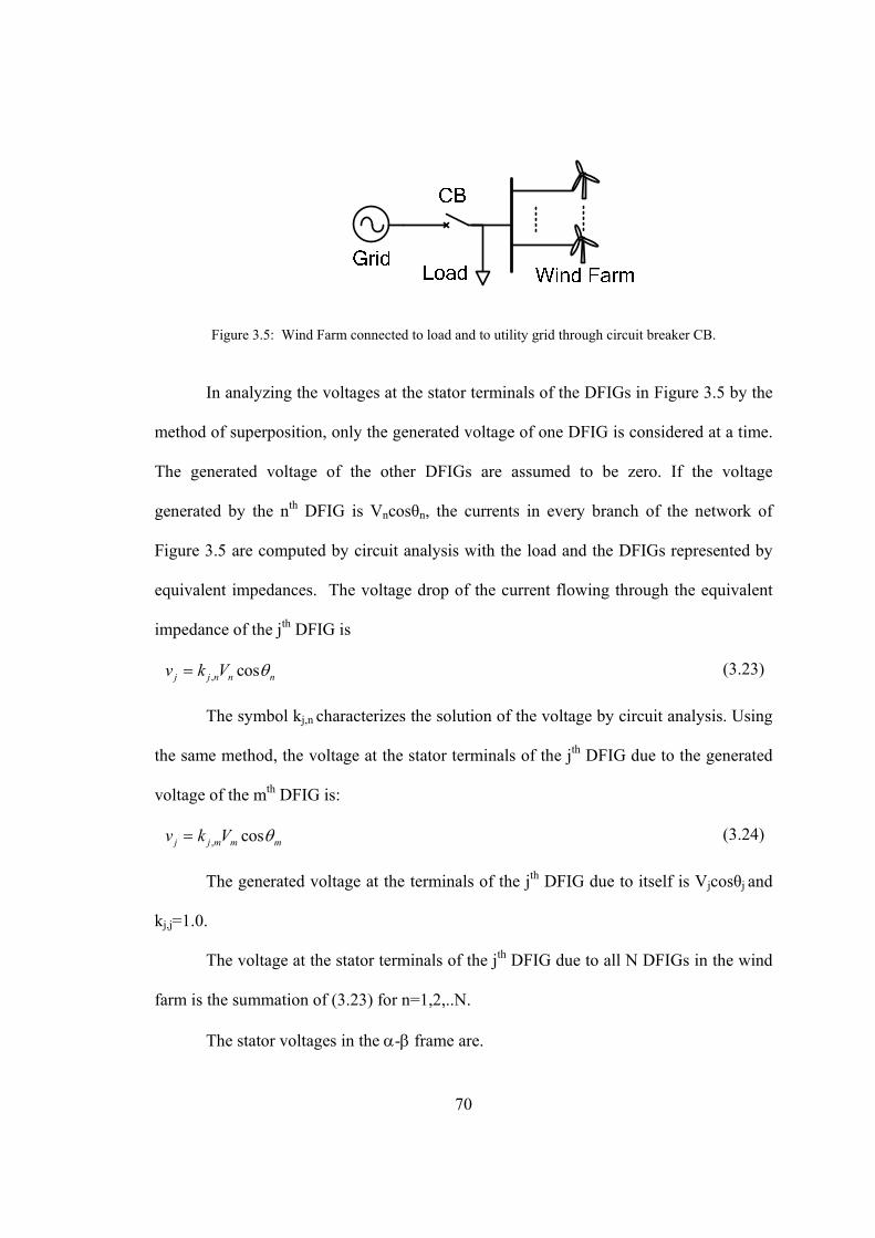
70
Figure 3.5: Wind Farm connected to load and to utility grid through circuit breaker CB.
In analyzing the voltages at the stator terminals of the DFIGs in Figure 3.5 by the
method of superposition, only the generated voltage of one DFIG is considered at a time.
The generated voltage of the other DFIGs are assumed to be zero. If the voltage
generated by the nth DFIG is Vncosθn, the currents in every branch of the network of
Figure 3.5 are computed by circuit analysis with the load and the DFIGs represented by
equivalent impedances. The voltage drop of the current flowing through the equivalent
impedance of the jth DFIG is
, cosj j n n nv k V (3.23)
The symbol kj,n characterizes the solution of the voltage by circuit analysis. Using
the same method, the voltage at the stator terminals of the jth DFIG due to the generated
voltage of the mth DFIG is:
, cosj j m m mv k V (3.24)
The generated voltage at the terminals of the jth DFIG due to itself is Vjcosθj and
kj,j=1.0.
The voltage at the stator terminals of the jth DFIG due to all N DFIGs in the wind
farm is the summation of (3.23) for n=1,2,..N.
The stator voltages in the - frame are.

71
,1
[ cos ]N
j n n nn
v k V
(3.25)
,1
[ sin ]N
j n n nn
v k V
(3.26)
The voltages of (3.25) and (3.26) are measured by the stator PLL of the jth DFIG.
From Figure 3.2, the error is
, ,sin cosj j v j vv v (3.27)
Substituting (3.25) and (3.26) in (3.27)
, ,1
[ sin( )]N
j j n n n j vn
k V
(3.28-a)
In (3.28-a), the n=j term takes the form
, ,sin( ) 0.0j j j j j vk V
This is because j=j,v+ and 0.0. Also, kj,j,=1.0. Therefore (3.28-a) can be
rewritten as
, , ,1
[ sin( )] sinN
j j n n n j v j j vn
k V V
(3.28-b)
Because of the sine functions in (3.28), a closed form solution of θj,v cannot be
found. However, if the frequencies and angles are close enough so that sin(n-j)(n-j),
(25-b) approximates to:
, ,1
[ ( )]N
j j n n n j v j jn
k V V
(3.29)
In practice, this approximation is reasonable because the PLLs of all the DFIGs
measure the utility grid frequency before it is lost, so that their frequencies are close
together just after islanding. When the negative feedback drives the error to j=0.0, the

72
stator PLL of the jth DFIG converges to
,1
,
,1
[ ]
[ ]
N
j n n n j jn
j v N
j n n jn
k V V
k V V
(3.30)
In wind farms where the DFIGs are identical, the lengths of lines are short and Q-
control is applied so that Vn (n=1,2..N) are identical, (30) simplifies to:
1,
[ ]
1
N
n jn
j v N
(3.31)
From (3.31), the PLL of every DFIG tracks the average of the voltage angles of
all the other DFIGs in the wind farm. In (3.31), all the angles n, n=1,2,..N, are time
varying functions. It is easier to demonstrate convergence graphically by converting
(3.31) into a sequence:
1,
[ ( )] ( )( 1)
1
N
n jn
j v
k kk
N
(3.32)
0 1 2 3 4 5 6 75
10
15
20
K
Figure 3.6: Illustration of convergence based on Equation (3.32)
Figure 3.6 is a graphical demonstration of convergence of the sequence of (3.32).
Starting with separate initial values, n(0), n=1,2,..6, the points of n(k) are shown for
k=0,1,2,..7. Convergence is reached by k=4. For readers who want a mathematical proof
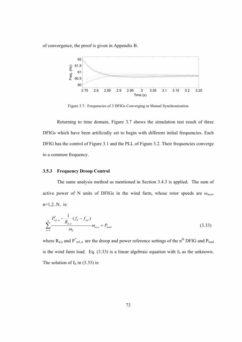
73
of convergence, the proof is given in Appendix B.
2.75 2.8 2.85 2.9 2.95 3 3.05 3.1 3.15 3.2 3.25
60
60.5
61
61.5
62
Fre
q. (
Hz)
Time (s)
Figure 3.7: Frequencies of 3 DFIGs Converging in Mutual Synchronization
Returning to time domain, Figure 3.7 shows the simulation test result of three
DFIGs which have been artificially set to begin with different initial frequencies. Each
DFIG has the control of Figure 3.1 and the PLL of Figure 3.2. Their frequencies converge
to a common frequency.
3.5.3 Frequency Droop Control
The same analysis method as mentioned in Section 3.4.3 is applied. The sum of
active power of N units of DFIGs in the wind farm, whose rotor speeds are m,n,
n=1,2..N, is:
*,
,,
1 0
1( )ref n S refN
d nm n load
n
P f fR
P
(3.33)
where Rd,n and P*ref,,n are the droop and power reference settings of the nth DFIG and Pload
is the wind farm load. Eq. (3.33) is a linear algebraic equation with fS as the unknown.
The solution of fS in (3.33) is:
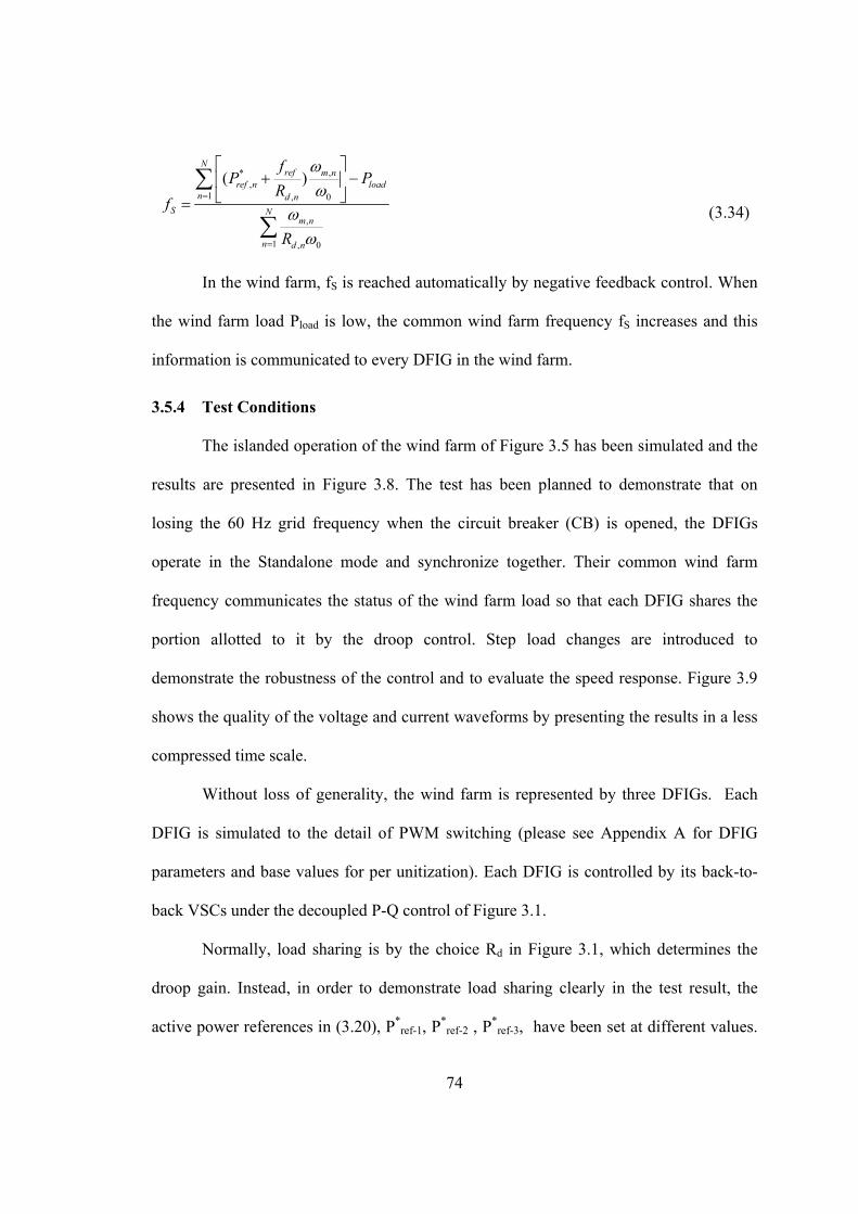
74
,*,
1 , 0
,
1 , 0
( )N
ref m nref n load
n d n
S Nm n
n d n
fP P
Rf
R
(3.34)
In the wind farm, fS is reached automatically by negative feedback control. When
the wind farm load Pload is low, the common wind farm frequency fS increases and this
information is communicated to every DFIG in the wind farm.
3.5.4 Test Conditions
The islanded operation of the wind farm of Figure 3.5 has been simulated and the
results are presented in Figure 3.8. The test has been planned to demonstrate that on
losing the 60 Hz grid frequency when the circuit breaker (CB) is opened, the DFIGs
operate in the Standalone mode and synchronize together. Their common wind farm
frequency communicates the status of the wind farm load so that each DFIG shares the
portion allotted to it by the droop control. Step load changes are introduced to
demonstrate the robustness of the control and to evaluate the speed response. Figure 3.9
shows the quality of the voltage and current waveforms by presenting the results in a less
compressed time scale.
Without loss of generality, the wind farm is represented by three DFIGs. Each
DFIG is simulated to the detail of PWM switching (please see Appendix A for DFIG
parameters and base values for per unitization). Each DFIG is controlled by its back-to-
back VSCs under the decoupled P-Q control of Figure 3.1.
Normally, load sharing is by the choice Rd in Figure 3.1, which determines the
droop gain. Instead, in order to demonstrate load sharing clearly in the test result, the
active power references in (3.20), P*ref-1, P
*ref-2 , P
*ref-3, have been set at different values.

75
In all the three DFIGs, Rd is set so that the droop gain is 0.3. The references in the
“Standalone Operation” block of Figure 3.1 are: Vref =1.0 pu and freq=60 Hz. Throughout
the test, the rotor speeds of the DFIGs are set constant at: m,1=0.9 pu, m,2=1.0 pu,
m,3=1.2 pu. The software tool used is: Matlab/Simulink.
3.5.5 Test Results
Figure 3.9 shows 4 graphs of: (a) VPCC the voltage at the PCC; (b) Igrid, the
current to the utility grid; (c) the wind farm frequency; (d)active powers delivered by the
three DFIGs.
0.8
1
1.2
|Vpc
c| (pu
)
-0.5
0
0.5
1
|I grid
| (pu
)
60
62
Fre
q. (
Hz)
2.5 3 3.5 4 4.5 5 5.5 6 6.5
0
0.2
0.4
Time (s)
Pow
er (
pu)
(a)
(b)
(c)
(d)
Figure 3.8: Wind Farm on Disconnection and Reconnection
(a), per-unitized voltage and current magnitudes at PCC; (b) magnitude of current to utility grid; (c) frequency; (d) active powers of individual DFIGs.
Before 3.0s
By t=2.5s, the steady-state has been reached by the simulation software. The wind

76
farm voltage is 1.0 pu. Igrid =0.36 pu. The DFIGs together produce 0.89 pu active power,
of which 0.53 pu goes to the local load and the remaining 0.36 pu to the utility.
3.0 s t 4.0s
At t=3.0 s, the CB is opened. As the utility grid load portion is cut off, the total
load of wind farm Pload in (3.34) is the local load of 0.53 pu active power. Because Pload in
(3.34) decreases, the wind farm frequency freq=fs rises. In each “Standalone Operation”
block, the increase in fs means that the power of the DFIG is decreased as required by
(3.20). The reduction of active powers from the three DFIGs is shown in the bottom
graph.
The effect of the step change on the waveforms of the voltages and currents of the
local load is shown in Figure 3.9.
4.0 s t 5.49s
In order to confirm the operation of the “Standalone Operation” block further, the
local load is given a step decrease at t=4.0. The frequency fS increases and the active
power outputs of the DFIGs decrease to match the decrease in load.
5.49 s t 6.5s
By 5.49s, it is assumed that the utility grid has recovered. The CB is closed by the
standard method described in the followed paragraph. Because the local load has been
decreased at t=4.0s, more of the DFIG active power is delivered to the utility grid so that
Igrid is larger than for t 3.0s. After the transient of the reconnection, the wind farm
frequency returns to 60 Hz and the active power outputs of the DFIGs return to values for
t 3.0s

77
The same procedure, which is used routinely to connect synchronous generators
to the utility grid, has been applied to reconnect the wind farm to the utility grid after it
has recovered. The utility grid voltage is available on the other side of the opened CB.
The voltage magnitudes on both sides have been set as 1.0 pu. The voltage across the CB
has a beat frequency (60-fS). The CB is closed when the voltage magnitude across the CB
drops to a minimum. As Figure 3.8 shows, the reconnection at t=5.49s is smooth.
-1
0
1
Vlo
ad (
pu)
2.98 2.99 3 3.01 3.02 3.03 3.04 3.05 3.06-1
0
1
Time (s)
I load
(pu
)
(a)
(b)
Figure 3.9: (a) Voltage (b) Current of Local Load
3.6 Incorporating Wind Velocity and Turbine Pitch Angle Control
When the wind farm is islanded, in general the wind turbines have a tendency to
accelerate because the load to the grid is disconnected so that the braking generating
counter-torque is lowered. To prevent over speeding, the pitch angle of the turbine blades
should open as fast as possible to spill wind.
3.6.1 Turbine Blade Pitch Controlled Wind Turbine Characteristics
The dynamics of the rotor speed m is governed by Newton’s 2nd Law of Motion
in the rotational frame:
mm e
dJ T T T
dt
(3.35)

78
where J is the equivalent moment of inertia, Tm is the wind turbine torque and Te is the
counter-torque of the DFIG. The wind turbine torque is
2 3( , ) ( , )p wind p air wmm
m m m
C P C r vPT
(3.36)
where Cp is the power coefficient of the wind turbine, r is the turbine radius (m), air is
the density of air and vW is the wind velocity (m/s). Cp is available from manufacturers in
the form of Cp-vs- curves such as shown in Figure 3.10 where is the tip speed ratio,
recalled the formula (2.44).
The Cp-vs- data of the manufacturer can be converted to Tm-vs-m
characteristics for any wind velocity. Figure 3.11 shows an example for vw=12 m/s and
one sees that Tm is lowered for =16, for example.
0 2 4 6 8 10 12 14 16 18 200
0.1
0.2
0.3
0.4
0.5
Tip Speed Ratio ()
Pow
er C
oeff
icie
nt (
Cp)
Power Coefficient Cp(, )
= 0o
= 2o
= 4o
= 6o
= 8o
=10o
=12o
=14o
=16o
Figure 3.10: Wind power coefficient Cp as a function of tip ratio for for different turbine blade pitch angle .

79
0.4 0.6 0.8 1 1.2 1.4 1.60
0.1
0.2
0.3
0.4
0.5
0.6
0.7
0.8
m (pu)
Tor
que
(pu)
Wind speed= 12 (m/s)
=0o
=2o
=4o
=6o
=8o
=10o
=12o
=14o
=16o
Figure 3.11: Wind torque Tm-vs-rotor speed m at wind speed vw=12m/s for different pitch angle .
3.6.2 Pitch angle control in standalone operation
From (3.35), dt
d m = am is acceleration, which can be measured by an accelerator.
If am > 0, ΔT > 0, the wind-turbine generator speeds up;
If am < 0, ΔT < 0, the wind-turbine generator slows down;
If am = 0, ΔT= 0, the wind-turbine generator maintains constant speed.
The signal am is applied to change β, the pitch angle of the turbine blades.
If am > 0, increase β in order to spill wind thus reducing ΔT when the wind-
turbine generator speeds up;
If am < 0, decrease β in order to increase ΔT to prevent the wind-turbine
generator from slowing down;

80
If am = 0, β is maintained so that ΔT= 0 keeps the wind-turbine generator
speed constant.
By adding the pitch angle control, the standalone DFIG wind farm can continue
powering the local load and keeping the generator shaft speed within the safety limits.
3.6.3 Test on Single WTG with Pitch Angle Control
In this test, the wind turbine is driven by wind velocity which is from a wind
velocity data file, shown graphically in Figure 3.12(a).
0 10 20 30 40 50 60
10
15
VW
1 (m
/s)
0 10 20 30 40 50 601
1.2
m
(pu
)
0 10 20 30 40 50 600
5
10
15
(
deg.
)
0 10 20 30 40 50 600.2
0.4
0.60.8
Time (s)
Tor
que
(pu)
Te
Tm
(a)
(b)
(c)
(d)
Figure 3.12: Simulation results of DFIG: (a) rotor speed m, (b) pitch angle , (c) wind turbine torque and
DFIG counter-torque, all in pu values.
By applying the pitch angle control strategy, the turbine speed ωm shown in
Figure 3.12 (b) is kept from exceeding the safety limit. Figure 3.12 (c) shows the
simulation of the pitch angle . As shown in Figure 3.12 (d) the pitch angle β is

81
controlled to balance the turbine torque Tm with the counter torque Te. As there is little
torque difference T in equation (3.35), the turbine speed is kept within the safe
permitted value.
From the electrical analysis point of view, the Figure 3.13 shows that the voltage
magnitude at PCC (a) maintains constant, the current flowed to the grid (b) is reduced to
zero after islanding, system frequency (c) increases to 60.49 Hz according to the droop
control, the total active power generated from DFIG (d) drops to 0.6 p.u. to match the
local load requirement.
5 10 15 20 25 30 35 40 45 50 55 600.8
1
1.2
Vpc
c Mag
. (p
u)
5 10 15 20 25 30 35 40 45 50 55 60
0
0.2
0.4
I pcc M
ag.(
pu)
5 10 15 20 25 30 35 40 45 50 55 60
60
60.5
Fre
quen
cy (
Hz)
5 10 15 20 25 30 35 40 45 50 55 60
0.5
1
Time (s)
PD
FIG
(pu
)
(a)
(b)
(c)
(d)
Figure 3.13: Simulation results of DFIG: (a) voltage magnitude at PCC, (b) current magnitude at local load , (c) system frequency, (d) total power output of DFIG

82
59.9 59.91 59.92 59.93 59.94 59.95 59.96 59.97 59.98 59.99 60-1
0
1
Vlo
ad (
pu)
59.9 59.91 59.92 59.93 59.94 59.95 59.96 59.97 59.98 59.99 60-1
0
1
Time (s)
I load
(pu
)(a)
(b)
Figure 3.14: Simulation results of DFIG: (a) local load voltage at PCC, (b) local load current
Figure 3.14 also shows the detailed information about the voltage (a) and current
(b) of the local load in three-phase format from 59.9 second to 60 second. The DFIG
with pitch angle control can maintain the system operated normally with variable wind
speed at islanding situation.
0 2 4 6 8 10 121
1.2
1.4
m
(pu
)
0 2 4 6 8 10 12-1
0
1
(
deg.
)
0 2 4 6 8 10 120.20.6
1
Tor
que
(pu)
0 2 4 6 8 10 12-0.5
00.5
1
Time (s)
To
rque
(pu
)
(a)
(b)
(c)
(d)
Te
Tm
Figure 3.15: Simulation results of DFIG: (a) rotor speed m, (b) pitch angle , (c) wind turbine torque and DFIG counter-torque, all in pu values.

83
The same simulation is repeated disabling pitch angle control block. One can see
the Figure 3.15 show that without pitch control, =0 in (b), the turbine speed in (a)
accelerates beyond the safe limit. Figure 3.15 (c) shows the wind turbine torque Tm (blue)
computed from (3.36) and the DFIG counter torque Te (red). Figure 3.15 (d) shows the
ΔT between Tm and Te larger than zero, that drives the wind turbine shaft speeding up.
3.6.4 Test on Islanding Capability of Wind Farm During Disconnection
Figure 3.5 illustrates the model of wind farm which is used in the simulations
tests. The wind farm is modeled by the same three DFIGs of the test of Figure 3.8. The
DFIGs are driven by pitch controlled wind-turbine with wind velocities given by Figure
3.16
0 10 20 30 40 50 60
10
15
VW
1 (m
/s)
0 10 20 30 40 50 60
10
15
VW
2 (m
/s)
0 10 20 30 40 50 60
10
15
Time (s)
VW
3 (m
/s)
(a)
(b)
(c)
Figure 3.16: Wind Velocities to WTGs
Islanding occurs at t=3.0 s. Prior to islanding Figure 3.17 shows, in: (a) the
frequency is 60 Hz from the utility grid; (b) the active power of each DFIG (PDFIG1,
84
PDFIG2, PDFIG3) is set by P*ref to be slightly lower than 0.3 pu; (c) the rotor speeds are set
slightly higher than 1.0 pu; (d) pitch angle =0.0.
After islanding, the general conclusions are:
(i) the WTGs synchronize to a common frequency of 60.6 Hz, as shown in (a);
(ii) PDFIG1, PDFIG2, PDFIG3 share the load in the same proportion as prior to
islanding as shown in (b);
(iii) the rotor speeds are kept below 1.2 pu (the targeted speed limit), as shown in
(c);
(iv) the speed limit is satisfied by increasing as shown in (d).
5 10 15 20 25 30 35 40 45 50 55 6059.5
60
60.5
61
61.5
Fre
quen
cy (
Hz)
5 10 15 20 25 30 35 40 45 50 55 600.1
0.2
0.3
PD
FIG
(pu
)
5 10 15 20 25 30 35 40 45 50 55 60
0.8
1
1.2
m
(pu
)
5 10 15 20 25 30 35 40 45 50 55 600
10
20
Time (s)
(
deg.
)
(d)
(c)
(a)
(b) PDFIG2
PDFIG1
PDFIG3
m3
m2
m1
1 2 3
Figure 3.17: (a) Wind Farm Frequency; (b) DFIG active power output; (c) rotor speeds; (d) pitch angles.

85
The local load, Pload, is half the power delivered prior to islanding. Prior to
islanding, the “Standalone Operation” block in Figure 3.1 is not activated and therefore
the wind farm takes the frequency of the utility grid. On islanding because Pload in (3.33)
has dropped, the common wind farm frequency fS increases. In the simulation in
“Standalone Operation” block, the frequency references are kept equal: fref,1=
fref,2=fref,3=60 Hz; and likewise the droop control Rd,1=Rd,2=Rd,3. The power references
P*ref,n, (n-1,2,3), are kept slightly unequal so that PDFIG1, PDFIG2 and PDFIG3 are distinct and
yet they can be seen to have divided the wind farm load power almost equally.
3.7 Conclusion
This chapter has shown that a standalone DFIG can have autonomous frequency
control. Furthermore, multiple units of such DFIGs synchronize to a common frequency
which is used with frequency droop control to share loads. The claims have been
validated by simulations. Because the common frequency originates from multiple
DFIGs, it is more reliable than one from a single master frequency. The increase in
reliability is obtained economically by adding the “Standalone Operation” block of
Figure 3.1 to new DFIGs or as retrofits to DFIGs already in service. The simulation has
demonstrated that a wind farm, based entirely on DFIGs, does not have to shut down
when the utility grid is lost. The wind farm can keep operating in a reserve mode, ready
to support the power system as soon as the utility grid has recovered.
Combined with pitch angle control of wind-turbine blades and autonomous
frequency control, DFIGs has the capability to serve in islanded situation where the

86
limited controls to balance stochastic loads against stochastic wind. The wind farm can
be operated within the safety speed limit.

87
Chapter 4: Adapting DFIGs for Operation as Doubly-Fed Induction
Motors (DFIMs)
4.1 Introduction
Doubly-fed induction generators, in sizes of 1.5 MW and higher, are widely used
as wind-turbine generators. They owe their popularity to the economic cost of their
rotor-side back-to-back VSCs which are rated to convey slip power only. This is because
for the range of rotor speed to capture most of the available wind power, the slip needs
only range from s=0.3 to s=-0.3. Therefore the size of the rotor-side VSCs can be reduced
to 0.3 times that of the stator-side VSCs giving DFIGs a considerable cost advantage. The
objectives of this chapter are to find out:
(i) how the existing design can be adapted for operation as motors with minimal
changes and
(ii) what are the marketable properties as motors.
Chapter 2 points out that over the years sensorless decoupled P-Q control has
been developed for DFIGs and this chapter shows how DFIMs can benefit from such
advances.
The parameters of a 1.5 MW DFIG intended for wind farms [68] from the base
for the adaptation. The back-to-back VSCs are rated at slip power of s=0.3. This chapter
refers to the explanation in Chapter 2, so as not to repeat descriptions of the - frame (d-
q frame used by other researchers) equations modeling the DFIG and descriptions of
decoupled P-Q control. In this chapter, it suffices to use the traditional induction machine
equivalent circuit which sacrifices neither accuracy nor rigor.

88
The contributions are:
(1) A graphical method of torque, current and speed analysis of DFIMs for
engineering design.
(2) Demonstration of low speed operation (-0.4 ≤ m≤ 0.7 pu) and
supersynchronous speed operation (1.3 ≤ m ≤ 2.0 pu) by auto-transformers.
(3) Demonstration of synchronization control to suppress switching torque
transients during circuit breaker closing.
(4) Demonstration of availability of continuously controllable reactive power.
(5) Demonstration of precision speed and position control by making use of rotor
position information which is available from the decoupled P-Q control inherited from
DFIGs.
Contributions (1), (2) and (3) have been necessitated by the fact that in order to
take advantage the economic size VSCs, the normal speed range is limited to 0.7 pu ≤ m
≤ 1.3 pu. Outside this speed range, the currents are excessively large so that reduced
stator voltage by autotransformers is required. The study shows there is substantial
accelerating torque after autotransformer voltage reduction.
Connecting the stator terminals of the DFIM to autotransformer terminals,
disconnecting them and reconnecting them directly to the ac grid terminals involve circuit
breaker switching. Switchings give rise to large oscillatory torque transients. Torque
transients have caused shaft breakages directly or by mechanical resonance [69].
Indirectly they shorten the life-time of the motor system through fatigue failure. The
authors have developed Synchronization Control for circuit breaker switching which is
shown to eliminate switching transients.

89
Because of the DFIM has decoupled P-Q control, the motor can run at unity
power factor. In addition, it can supply capacitive reactive power to compensate the
inductive reactive power of an industrial plant. One is reminded that reactive power
compensation is often the second reason for the purchase of large synchronous motors.
The ability to implement decoupled P-Q control implies that the controller has
already a rotor position sensor (incremental or absolute position sensor or a sensorless
means). These sensors can be used by DFIMs to operate as precision speed and/or
position controllers.
Research on DFIM dates back to days when wound rotor induction motors with
power electronic control came under the name of static Scherbius drives [70-73]. Then,
as now, the research has been on the technologies and the methods to manage of slip
power mostly in the slip range of 0.0 ≤ s ≤ 1.0. The research follows in the footsteps of
pioneers in the supersynchronous speed range -1.0 ≤ s ≤ 0.0 [74]. Since DFIGs took off
in wind power applications, interest has been focused on operation as generators in the
slip range of -0.3 ≤ s ≤ 0.3 [75-77]. The research is focused on motor application in the
slip range of -1.0 ≤ s ≤ 1.4 ( -0.4 pu ≤ m ≤ 2.0 pu) while using the economic converters
rated for operation in the slip range of -0.3 ≤ s ≤ 0.3 (0.7 ≤ m ≤ 1.3).
The chapter is organized as follows: Section 4.2 develops on the traditional
equivalent circuit of the induction machine, which shows that the DFIM is a hybrid of an
asynchronous motor and a synchronous motor. Like the synchronous motor, the DFIM
can control both real and reactive power. Unlike the synchronous motor, the rotor speed
is not restricted to operation at synchronous speed only. Section 4.3 presents (Te, Is)
diagrams to guide the adaptation of the DFIG to DFIM. Section 4.4 shows that the

90
limitation from under-rated converter size can be off-set by autotransformers. Section 4.5
draws attention to torque transients arising from circuit breaker switching as
autotransformers are connected and disconnected. Section 4.6 describes the
synchronizing control which is used in conjunction with circuit breakers to eliminate
switching torque transients. Section 4.7 draws attention to the availability of reactive
power. Section 4.8 presents precision speed and position control. Experimental results to
confirm some of the simulation results given in Section 4.9.
4.2 Steady-State Treatment of Doubly-Fed Induction Motor
4.2.1 Equivalent Circuit Analysis Modern treatment on doubly-fed induction machines make use of the -
reference frame as this thesis has also done in the development of decoupled P-Q control
[39-41]. The traditional per-phase equivalent circuit shown in Figure 4.1 is sufficient for
this chapter. Reference [78] has shown that DFIG/DFIM is more easily understood,
without loss of accuracy, as a hybrid of the induction (asynchronous) machine and the
synchronous machine. In Figure 4.1, the rotor resistance, /RR s , accounts for the
asynchronous motor portion of the hybrid and the rotor-side voltage from the inverter,
/RE s , accounts for the synchronous motor portion.
Figure 4.2 shows further partitioning of /RR s and /RE s . For the asynchronous
motor portion, RR accounts for ohmic loss 2
3 R RR I and [(1/ ) 1]RR s accounts for
conversion to mechanical power 2
3 ((1/ ) 1)e asy m R RT R s I where e asyT is the
asynchronous motor torque component. Likewise for the synchronous motor portion, RE

91
represents the slip power *Re{3 }R RE I entering the rotor windings and
[(1/ ) 1]RE s accounts for conversion to mechanical power *Re3 [(1/ ) 1]e syn m R RT E s I
where e synT is the synchronous motor torque component of the hybrid. The shaft torque of
the DFIM is e e asy e synT T T .
In Figure 4.1 and 4.2, the frequency of RE is 60 Hz because the equivalent
circuits are referenced to the stator side.
SI~
Mj
Sj Rj
SE~
RE
s
RR
sSR
RI~
Figure 4.1: Equivalent circuit of DFIM
RI~
Mj
Sj Rj
RR
SE~
SRRE
~
1
1~s
ER
1
1
sRR
SI~
RS II~~
Figure 4.2: Circuit elements inside box account for electromechanical energy conversion.
In analyzing the DFIM, one begins with knowledge of the stator side voltage SE ,
rotor side voltage RE and rotor speed m and proceed to solve for the loop currents
SI and RI of the equivalent circuit as a standard circuit theory problem. The electrical
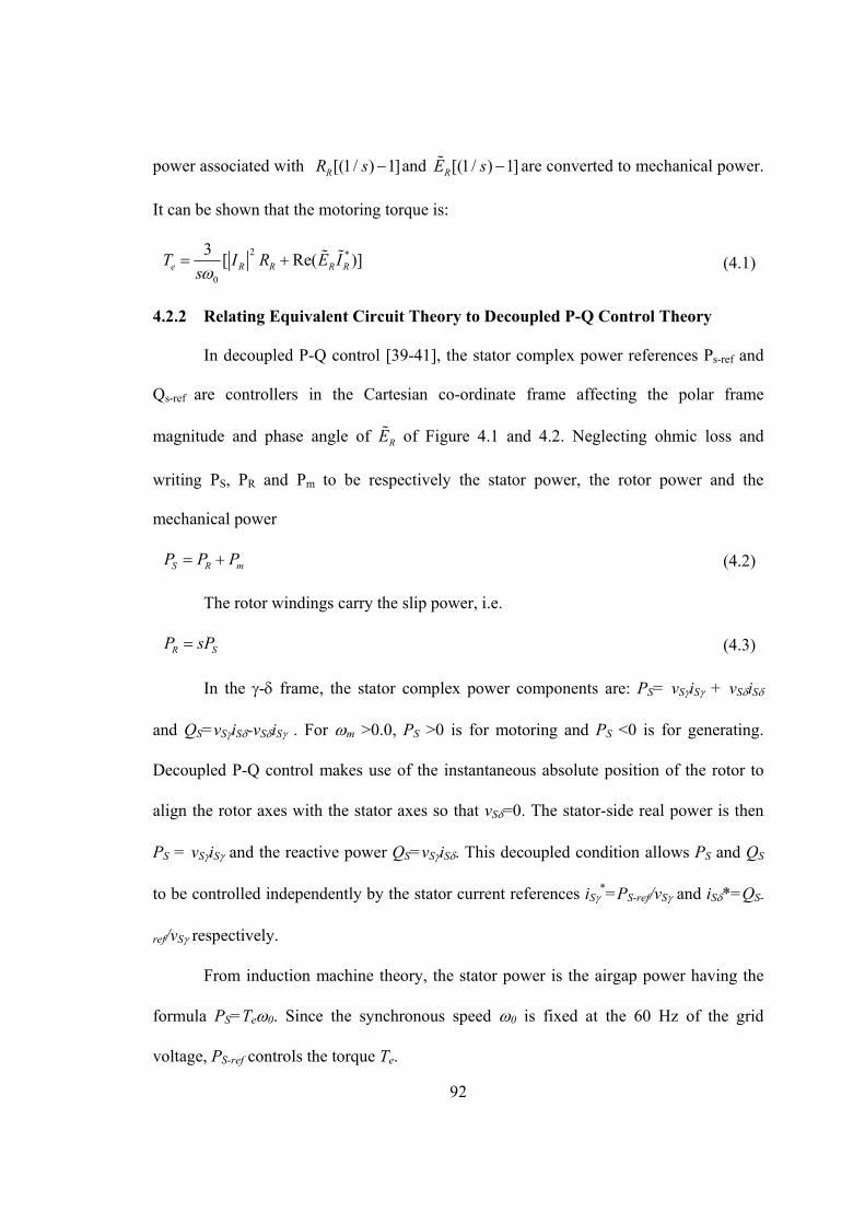
92
power associated with [(1/ ) 1]RR s and [(1/ ) 1]RE s are converted to mechanical power.
It can be shown that the motoring torque is:
2 *
0
3[ Re( )]e R R R RT I R E I
s (4.1)
4.2.2 Relating Equivalent Circuit Theory to Decoupled P-Q Control Theory
In decoupled P-Q control [39-41], the stator complex power references Ps-ref and
Qs-ref are controllers in the Cartesian co-ordinate frame affecting the polar frame
magnitude and phase angle of RE of Figure 4.1 and 4.2. Neglecting ohmic loss and
writing PS, PR and Pm to be respectively the stator power, the rotor power and the
mechanical power
S R mP P P (4.2)
The rotor windings carry the slip power, i.e.
R SP sP (4.3)
In the - frame, the stator complex power components are: PS= vSiS + vSiS
and QS=vSiS-vSiS . For m >0.0, PS >0 is for motoring and PS <0 is for generating.
Decoupled P-Q control makes use of the instantaneous absolute position of the rotor to
align the rotor axes with the stator axes so that vS=0. The stator-side real power is then
PS = vSiS and the reactive power QS=vSiS. This decoupled condition allows PS and QS
to be controlled independently by the stator current references iS*=PS-ref/vS and iS*=QS-
ref/vS respectively.
From induction machine theory, the stator power is the airgap power having the
formula PS=Te0. Since the synchronous speed 0 is fixed at the 60 Hz of the grid
voltage, PS-ref controls the torque Te.

93
4.3 Relating DFIM with VSCs Rated for s=0.3 Slip Power
The research is concerned with keeping the design of the 1.5 MW DFIG and its
VSCs unchanged. As the VSCs are rated to carry s=0.3 slip power, the rotor voltage
magnitude is economically limited to ER ≤0.3 pu. Since the rotor voltage is /RE s in
Figure 4.1, for DFIG speed range 0.7 ≤ m ≤ 1.3 pu , ER = 0.3 is satisfactory because
ER/s=0.3/0.3=1.0, which is compatible with the supply voltage ES = 1.0. However, for
the motor during start at m = 0.0, when s =1.0, the VSC output voltage of ER = 0.3
means that ER/s=0.3/1.0=0.3, which is a low voltage compared with the supply voltage
ES=1.0. The large difference in the voltages means that the resultant currents would
exceed machine rating. Therefore it is necessary to address operation outside the speed
range favourable to wind power application.
To help in the analysis, Te-vs-Is diagrams have been developed in Figure 4.3, 4.4,
4.6 and 4.7. In these diagrams, Te >0 is for motoring and Te <0 is for generating. The x-
axis of the diagrams is for the magnitude of stator current IS solved from the equivalent
circuit of Figure 4.1. From the solution of currents, the torque Te is computed by (4.1)
and this datum is plotted against the y-axis. All the figures are based on machine
parameters taken from the 1.5 MW DFIG of [68].
Figure 4.3 is for speed m=0.0 and stator voltage magnitude Es=1.0 pu. Each
ellipse is the locus of (Te, IS) points solved for one magnitude of the rotor voltage RE (for
0.0 ≤ ER ≤0.3 pu) for 360 rotation of the voltage angle. The envelope of 0.3RE is
drawn in bold. All the (Te, IS) points for ER ≤0.3 pu lie inside the envelope drawn in bold.
In Figure 4.3, it is clear that the rated operating point (Te-rate=4770 Newton-Meters,
Irate=1250 A) cannot be reached by ER ≤0.3 pu, when Es=1.0 pu. The loci of rated

94
current Irate and rated torque Te-rate are drawn as vertical and horizontal lines respectively
in Figure 4.3 and Figure 4.4.
0 500 1000 1500 2000 2500 3000 3500 4000 4500-4000
-2000
0
2000
4000
6000
8000
10000
12000
Tor
que
(N.M
)
Is (A)
Irate
Te-rate
Figure 4.3: Torque-vs-Stator Current (ES=1.0 pu, 0.0≤ ER≤ 0.3 pu, m=0.0)
0 1000 2000 3000 4000 5000 6000-6
-4
-2
0
2
4x 10
4
Tor
que
(N.M
)
Is (A)
Te-rate
Irate
m=1.0
m=1.3
m=0.7
Figure 4.4: Torque-vs-Stator Current (ES=1.0 pu, 0.0≤ ER ≤ 0.3 pu, for m=0.7 pu and envelopes of m=1.0 pu and m=1.3 pu.)
Figure 4.4 shows three sets of the locii of Figure 4.3: for speeds m=0.7 pu,
m=1.0 pu and m=1.3 pu. The ellipses of 0.0≤ ER ≤ 0.3 pu are depicted in Figure 4.3 for
m=0.7 pu. For m=1.0 pu and m=1.3 pu, only the envelopes are drawn. The rated
95
operating point (Te-rate, IS-rate) lies within the envelopes. Figure 4.4 confirms that the
DFIM can operate in the speed range 0.7≤ m≤ 1.3 pu when ES=1.0 pu and 0.0≤ ER ≤ 0.3
pu and output the rated torque of 4770 newton-meters at rated current 1250 A.
4.4 Adapting DFIG for DFIM Application
In wind farm operation, the wind accelerates the turbine past 0.7 pu speed after
which the DFIG is synchronized to the grid. In contrast, the DFIM must use its own
motoring torque to accelerate from standstill to 0.7 pu speed so as to take advantage of
ER ≤ 0.3 pu. From Figure 4.3, the starting currents are prohibitively large.
m
mT
Figure 4.5: Schematic of Doubly-Fed Induction Motor with autotransformer.
Borrowing from industrial practice of starting with line voltages reduced by
autotransformers, a standard size autotransformer rated at ES=0.5 pu is considered. Figure
4.5 shows the single-line schematic of the DFIM with an autotransformer for voltage
reduction.
Figure 4.6 and Figure 4.7 show the (Te,IS) diagrams for ES=0.5 pu, 0≤ ER≤ 0.3 pu.
From the envelopes of Figure 4.6, one sees that operation at the rated current of around
1250 A is possible from negative speed of -0.4 pu to positive speed of 0.6 pu. Although

96
the motoring torque is below the rated 4770 N-m, it should be sufficient for acceleration
to reach 0.7 pu speed.
0 500 1000 1500 2000 2500 3000 3500 4000-1
-0.5
0
0.5
1x 10
4T
orqu
e (N
.M)
Is (A)
m=0.6
m=0.4
m=0.2
m=0.0
m= -0.2
m= -0.4
Te-rate
Irate
Figure 4.6: Envelopes of Torque-vs-Stator Current (ES=0.5 pu, 0≤ ER≤ 0.3 pu, for -0.4 ≤m≤ 0.6 pu)
0 500 1000 1500 2000 2500 3000 3500 4000-15000
-10000
-5000
0
5000
Tor
que
(N.M
)
Is (A)
m=1.4
m=1.6
m=2.0m=1.8
Irate
Te-rate
Figure 4.7: Envelopes of Torque-vs-Stator Current (ES=0.5 pu, 0≤ ER≤ 0.3 pu, for 1.4 ≤m≤ 2.0 pu)
Figure 4.7 shows that if the autotransformer is re-inserted in the range 1.4 ≤m≤
2.0 pu, the rated current is not exceeded although the rated torque is not attained.

97
4.5 Switching Transients in Large Electric Machines
There is a literature on switching torque transients of synchronous generator [79]
and induction machines [80-82] because their peak torque magnitudes can be many times
larger than the rated values. The torque transients have the potential to shorten the life-
time of the machine through fatigue failure. Induction motor starting is accompanied by a
component which oscillates at line frequency which can lead to forced resonance if the
shaft system has a mechanical resonance close to it [69].
Figure 4.8 shows the result of a simulation in which the DFIM after exceeding m
=0.7 p.u. has been disconnected from the autotransformer. At t=3s, the DFIM is
connected directly to the AC grid. At the same time Pref (which controls the torque
directly) is increased linearly and then held constant.
Figure 4.8 shows that there is a large torque transient due to switching at t=3s.
1 2 3 4 5 6 7-2
-1.5
-1
-0.5
0
0.5
1
1.5x 10
4
Time (s)
Tor
que
(N.m
)
Figure 4.8: Simulation of DFIM torque: connected to the grid at speed m=0.8pu. 4.6 Synchronization control to Suppress Switching Transients
4.6.1 Principle of Synchronization Control

98
The method of suppressing switching transients is borrowed from the well known
technique of synchronizing alternators on line. This is by making the machine-side
voltages identical to the line-side voltages equal so that on closing the circuit breaker the
resultant currents are zero.
Figure 4.9 shows a schematic where a Synchronization Control block is added to
the block of decoupled P-Q control schematic taken from [39]. The superscript * is used
to designate a control variable; for example, the stator active and reactive power
controllers are P*S and Q*
S. The stator active and reactive power references are P*ref and
Q*ref. The measured active and reactive powers used for negative feedback are PS and QS.
The Synchronization Control block takes measurements of grid voltages (vga, vgb, vgc) and
the voltages of the stator terminals (vsa, vsb, vsc). Although the circuit breakers are open,
there are stator voltages because they are induced from the magnetizing currents excited
by the rotor side VSCs which are powered from the grid-side of the circuit breakers
shown as Figure 4.5. The voltages of the stator terminals (vsa, vsb, vsc) yield θs from the
stator PLL and the voltage magnitude Vs. The grid voltages (vga, vgb, vgc) are processed
to yield the magnitude Vgrid and phase angle θgrid. The angles and magnitudes of the
voltages are compared and the errors θ and v are applied to P*s and Q*
s control the rotor
voltages (vra, vrb, vrc) which in Figure 4.1 and 4.2 are represented by RE . The magnitude
and the phase angle of RE are changed in negative feedback to null the errors θ and v .
After the voltages are synchronized, the circuit breakers are closed. Because θ =0.0 and
v =0.0, it is not necessary to disconnect the Synchronization Control block.

99
r abci
r abcv
ri
ri*ri
*ri
*rv*rv
*si
*si
1
sje
m
s
SP SQ*
refP *refQ
1
m sL
* *ref refP Q Ref.
Generators s
Measured
P and Q
sV
sV
gridV*
sP *sQ
sje
s
V
1
abc
abc
s abcv
grid
m
mje
mje
s
Figure 4.9: Schematic of decoupled P-Q control with Synchronization Control added. 4.6.2 Test on Synchronization Control
Because the majority of DFIGs employ mechanical position sensors (incremental
or absolute position encoders), it needs to be pointed that their information on rotor
position r is inputted in the block, “Rotor Position Sensor” in Figure 4.9. Furthermore,
the simulations and experimental tests are based on using a position encoder to
emphasize that Synchronization Control and other operations do not depend on the Rotor
Position PLL [39].
The simulated results in Figure 4.10 show that automatic synchronization of the
stator voltages with those of the grid is successfully accomplished by Synchronization
Control. Figure 4.10 (a) and (b) are respectively the simulated voltages of the 3-phase ac
grid and the stator terminals of the DFIM. The function of Synchronization Switching
Control is to ensure that the terminal voltages of the DFIM are identical in magnitude,
frequency and phase with those of the grid. In (b) the voltage spikes come from the
switching by the IGBTs of the rotor side VSCs. After t=3.0s, when the circuit breaker is
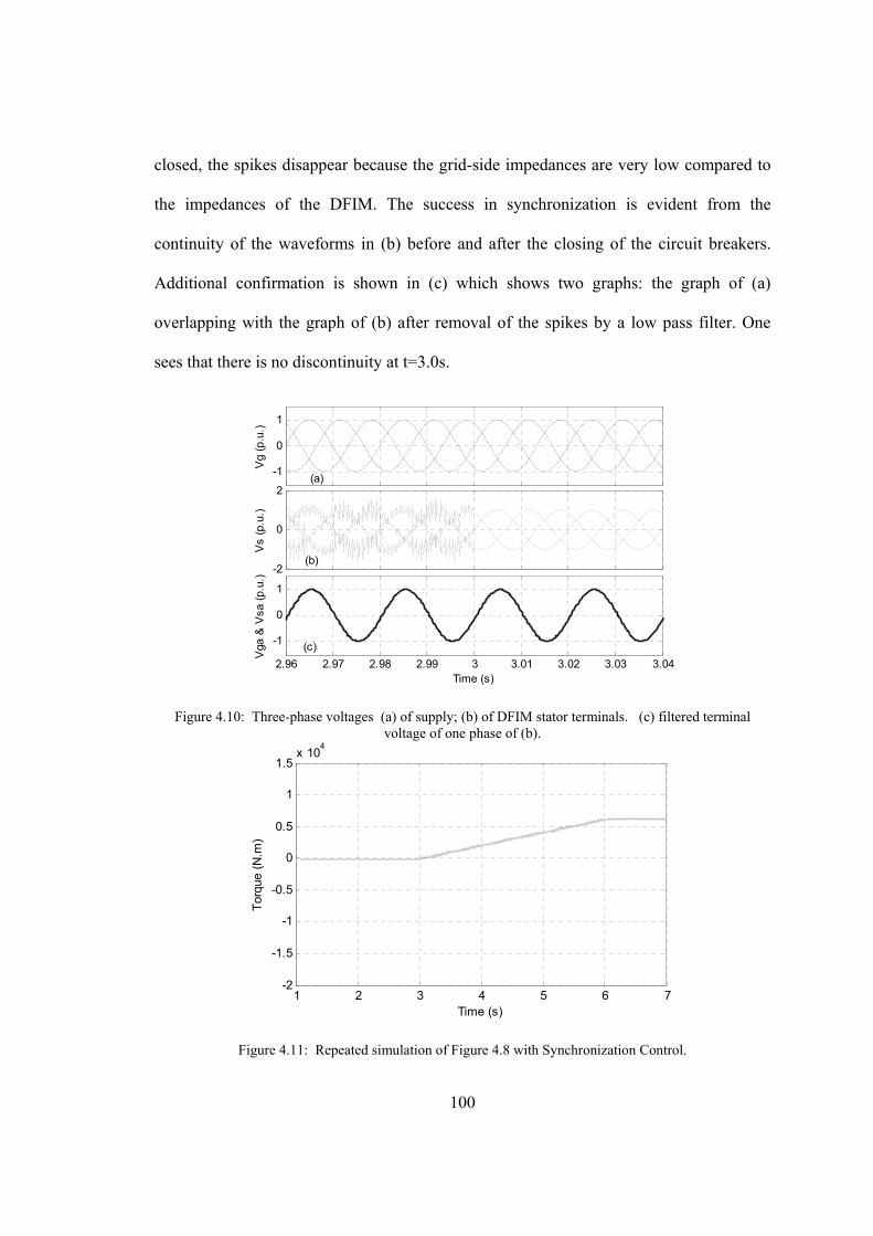
100
closed, the spikes disappear because the grid-side impedances are very low compared to
the impedances of the DFIM. The success in synchronization is evident from the
continuity of the waveforms in (b) before and after the closing of the circuit breakers.
Additional confirmation is shown in (c) which shows two graphs: the graph of (a)
overlapping with the graph of (b) after removal of the spikes by a low pass filter. One
sees that there is no discontinuity at t=3.0s.
-1
0
1
Vg
(p.u
.)
-2
0
2
Vs
(p.u
.)
2.96 2.97 2.98 2.99 3 3.01 3.02 3.03 3.04
-1
0
1
Time (s)
Vga
& V
sa (
p.u.
)
(a)
(b)
(c)
Figure 4.10: Three-phase voltages (a) of supply; (b) of DFIM stator terminals. (c) filtered terminal voltage of one phase of (b).
1 2 3 4 5 6 7-2
-1.5
-1
-0.5
0
0.5
1
1.5x 10
4
Time (s)
Tor
que
(N.m
)
Figure 4.11: Repeated simulation of Figure 4.8 with Synchronization Control.

101
The simulation experiment of Figure 4.8 has been repeated with Synchronized
Control. It yields the torque output shown in Figure 4.11. There is no torque transient of
the type reported in [21]-[23]. The torque transient in Figure 4.8 has been eliminated.
4.7 Reactive Power Control
The simulation result in Figure 4.12 confirms that reactive power, which is
obtainable in DFIGs, is also available the DFIM. Figure 4.13 also confirms decoupled P-
Q control because the active power is held constant at PS=0.8 pu throughout the
simulation experiment while QS is commanded to deliver zero, steps of negative and
positive reactive power. Within the stator MVA rating, one can obtain QS=(1-0.82)=
0.6 pu for PS=0.8 pu. It should be added that the reactive power is also available from
the grid-side VSC of Figure 4.5. Controllable QS also means that unity factor operation at
all the time is possible.
-1
-0.5
0
0.5
1
Ps (
p.u.
)
1 2 3 4 5 6 7-1
-0.5
0
0.5
1
Time (s)
Qs (
p.u.
)
Figure 4.12: Simulations showing decoupled control of P-Q in DFIM
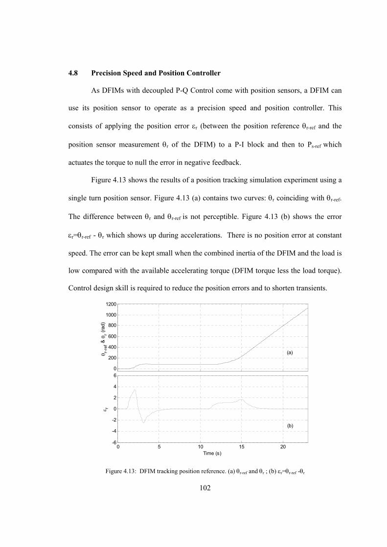
102
4.8 Precision Speed and Position Controller
As DFIMs with decoupled P-Q Control come with position sensors, a DFIM can
use its position sensor to operate as a precision speed and position controller. This
consists of applying the position error r (between the position reference r-ref and the
position sensor measurement r of the DFIM) to a P-I block and then to Ps-ref which
actuates the torque to null the error in negative feedback.
Figure 4.13 shows the results of a position tracking simulation experiment using a
single turn position sensor. Figure 4.13 (a) contains two curves: r coinciding with r-ref.
The difference between r and r-ref is not perceptible. Figure 4.13 (b) shows the error
r=r-ref - r which shows up during accelerations. There is no position error at constant
speed. The error can be kept small when the combined inertia of the DFIM and the load is
low compared with the available accelerating torque (DFIM torque less the load torque).
Control design skill is required to reduce the position errors and to shorten transients.
0
200
400
600
800
1000
1200
r-r
ef &
r (
rad)
0 5 10 15 20-6
-4
-2
0
2
4
6
Time (s)
r
(b)
(a)
Figure 4.13: DFIM tracking position reference. (a) r-ref and r ; (b) r=r-ref -r

103
Figure 4.14 shows another tracking experiment in which r-ref is assumed to be
from the position sensor on a Master motor and r is from the sensor of the DFIM acting
as a Slave. This simulation involves Multi-turn position sensors. The Slave starts about 1
second after the Master has departed. Eventually the Slave catches up and tracks the
Master with zero position error when the speed in constant and when the Master is at rest
in a new position.
Both Figure 4.13 and 4.14 demonstrate that DFIMs, with decoupled P-Q control
capability, have the potential to be used as precision speed and position controllers.
0
200
400
600
800
r-r
ef &
r (
rad)
0 2 4 6 8 10 12 14 16-20
0
20
40
60
Time (s)
r
r
r-ref
(b)
(a)
Figure 4.14: Multi-turn position reference tracking. (a) r-ref and r ; (b) r=r-ref -r
4.9 Laboratory Test Results
4.9.1 Experimental Test on 4-Quadrant Capability
The laboratory is equipped with a 5 hp 1700 rpm wound rotor induction machine
mechanically coupled to a separately excited 3.5 kW 1750 rpm dc machine to form a
dynamometer test bed. Since diagrams of the experimental layout and the photos of the

104
dynamometer appear in [8], they are not reproduced here. Appendix A.2 lists the
parameters of the two machines.
The test, whose results are shown in Figure 4.15, has been conducted to show that
the DFIM is capable of 4-quadrant operation under decoupled P-Q control. The
experiment has been conducted with autotransformer to show that the DFIM has an
extended speed range to 2.0 pu. It has also a negative speed range with autotransformer.
-1
0
1
2
Spe
ed (
p.u.
)
80 100 120 140 160 180
-500
0
500
1000
Time (s)
Pow
er (
W)
Ps
Ps-ref
(a)
(b)
Figure 4.15: (a) Speed; (b) Stator power PS and reference setting Ps-ref, in 4-Quadrant Test
At about 75.4s, with active power setting of Ps-ref=+600watts, the DFIM drives the
DC machine (load) from standstill to 2.0 pu speed as recorded in (a). As shown in (b), the
measured stator-side power (which has noise from the IGBT switchings) tracks the
reference setting, Ps-ref. When the speed reaches 2.0 pu, the power reference is changed
to Ps-ref = -250 watts as shown in (b). The DFIM operates in the regenerative braking
mode. The negative DFIM torque and friction brakes the system to zero speed.
At 130s, the negative torque continues to decelerate the rotor past zero speed and
the DFIM accelerates in the negative direction. At the time 182.6s, the reference is set to
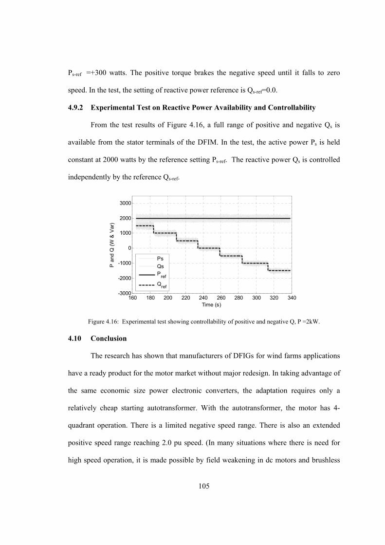
105
Ps-ref =+300 watts. The positive torque brakes the negative speed until it falls to zero
speed. In the test, the setting of reactive power reference is Qs-ref=0.0.
4.9.2 Experimental Test on Reactive Power Availability and Controllability
From the test results of Figure 4.16, a full range of positive and negative Qs is
available from the stator terminals of the DFIM. In the test, the active power Ps is held
constant at 2000 watts by the reference setting Ps-ref. The reactive power Qs is controlled
independently by the reference Qs-ref.
160 180 200 220 240 260 280 300 320 340-3000
-2000
-1000
0
1000
2000
3000
Time (s)
P a
nd Q
(W
& V
ar)
Ps
QsP
ref
Qref
Figure 4.16: Experimental test showing controllability of positive and negative Q, P =2kW. 4.10 Conclusion
The research has shown that manufacturers of DFIGs for wind farms applications
have a ready product for the motor market without major redesign. In taking advantage of
the same economic size power electronic converters, the adaptation requires only a
relatively cheap starting autotransformer. With the autotransformer, the motor has 4-
quadrant operation. There is a limited negative speed range. There is also an extended
positive speed range reaching 2.0 pu speed. (In many situations where there is need for
high speed operation, it is made possible by field weakening in dc motors and brushless

106
dc motors.) For duties which have frequent starts and stops, regenerative braking
contribute to energy saving. Switching torque transients can be suppressed by using
Synchronization Control in conjunction with circuit breaker switching. The DFIM has
continuously controllable positive and negative reactive power. Unity power factor
operation is possible. (Large synchronous motors are often purchased because the
capacitive reactive power is used to compensate the inductive VARs of induction motors
of the plant.) DFIMs, with decoupled P-Q control, offer precision speed and position
control capability.

107
Chapter 5: Conclusions
5.1 Summary
DFIGs, in the 1.5 MW to 3.0 MW range, are widely used in modern wind farms
because their power electronic controllers need only be rated at the maximum slip
frequency of 0.3pu and therefore they are cheaper. The research of this thesis has
addressed problems which still need to be attended to, chapter by chapter.
Chapter 2: When DFIGs operate under decoupled P-Q control, it is required that
its rotor position is accurately measured. Mechanical position transducers are widely
used. Many wind farms are located remotely under harsh environment so that failures in
mechanical sensors are not uncommon. A non-mechanical (“sensorless means”) method
based on the invention of Rotor Position Phase Lock Loop has been offered as
alternative.
Chapter 3: When the utility grid has a fault, the circuit breakers of the wind farm
open and the wind farm is said to be “islanded”. In the past, the islanded wind farm shuts
down. But with better controllability, wind farms are expected to keep operating as
reserve so that when the weakened utility grid recovers, the wind farms can assist in fast
restoration. This chapter shows that a DFIG has not only standalone capability but also
the capability to generate autonomous ac voltages with controllable frequency. This
chapter has also addressed the critical initial period of islanding when there is excess
wind power because the load to the utility is cut off.
Chapter 4 shows that the advances developed for DFIGs have marketable value as
Doubly-Fed Induction Motors.

108
5.2 Conclusion
5.2.1 Chapter 2
This chapter has described the principle of operation of the Rotor Position Phase
Lock Loop, which acquires the rotor position and rotor speed simultaneously, both of
which are vital information for the implementation of decoupled P-Q control in the
DFIG. The analysis shows that the Rotor Position PLL is robust because the
magnetization reactance of the DFIG is the only information required for it to operate in
the full range. In fact, a coarse estimate of the magnetization inductance is sufficient.
Unlike other “sensorless methods” which must depend on accurate parameter values,
there is no performance deterioration associated with winding resistance changes with
temperature or inductance changes with saturation. The Rotor Position PLL has passed
tests in an environment containing harmonics arising from unbalance and saturation of
iron. An analysis has been presented explaining why it is insensitive to noise.
There exist claims of sensorless Maximum Power Point Tracking (MPPT) of
wind power. These claims simply mean that the anemometer is not used to measure wind
speed. In decoupled P-Q controlled DFIG, rotor position tracking is obligatory so that
when a position encoder is used, the claim is genuine. Simulations using wind velocity
from a data file has shown that true sensorless MPPT is achievable without anemometer
and without mechanical position encoder (but using Rotor Position PLL ).
Laboratory tests have been made with a wound-rotor induction motor controlled
by back-to-back voltage-source converters. The experimental tests in a noisy
environment are strong proofs that the Rotor Position PLL is robust and insensitive to
109
measurement noise and it can provide the accurate speed and position information to
implement de-coupled P-Q control of the DFIG.
5.2.2 Chapter 3
Firstly, a DFIG is shown to be able to operate in standalone mode by adding a
“Standalone Operation” block to the original control design which implements decoupled
P-Q control. By a succession of innovations, the DFIG is shown to have: (i)
“autonomous frequency” control capability, (ii) the ability to synchronize to an islanded
grid frequency with other similarly designed DFIGs, (iii) the ability to share loads by
frequency droop concept.
These capabilities have been demonstrated by simulations. In addition, (i) the
principle underlying autonomous frequency control has been demonstrated by Phase
Plane Method; (ii) the principle underlying synchronizing to a common islanded grid
frequency has been demonstrated analytically.
The research has identified that before the wind farm reaches the steady state
when the DFIGs synchronize and share loads, it must survive power imbalance in the
first instants of islanding. Because the utility load is cut off, the excess wind power will
accelerate the wind turbines above the safe turbine speed limit. The simulation study
shows that a combination of fast turbine blade pitch angle control (to spill wind),
generator counter-torque from local electrical load (to brake the acceleration), large
moment of inertia of wind turbine blades (to decrease the rate of acceleration), the
accelerating wind turbine generators can be restrained to operate within the safe speed
limit.

110
5.2.3 Chapter 4
Chapter 4 shows that DFIGs designed for wind farms can be adapted for the
motor market by adding a relatively cheap starting autotransformer. DFIMs are shown to
have four quadrant capability by controlling the power electronic converters of DFIGs.
The speed and position transducers or “sensorless Means” required by decoupled P-Q
control can be used for precision speed and position control in the motoring applications.
Many large synchronous motors are purchased for their power factor correction
capability. DFIM is shown to be capable of supplying capacitive reactive power. The
ability of reactive power control by the DFIM is proved by experimentally in the
laboratory.
A Synchronization Control has been proposed to eliminate transient torque
oscillation during switching.
5.2.4 Future Work
The techniques developed for DFIGs in islanded wind farms has broader
applications in wind farms which are based on synchronous generators and permanent
magnet generators. Islanding is a general problem of renewable energy and distributed
generation.

111
References
[1] Canadian Wind Energy Association (CanWEA), Canadian Wind Farms: “Powering
Canada's Future, June 2012”, http://www.canwea.ca/pdf/Canada Current Installed Capacity_e.pdf
[2] J.G Slootweg, “Wind power: modeling and impact on power system dynamic,”
Ph.D. thesis, Delft University of Technology, Delft, Netherlands, 2003 [3] V. Akhmatov, “Analysis of dynamic behavior of electric power systems with large
amount of wind power,” Ph.D. thesis, Electric Power Engineering, Orsted- DTU, Tech. University, Denmark, Kgs. Lyngby, 2003
[4] V. Akhmatov, “Variable-speed wind turbines with doubly-fed induction generators;
Part I: Modelling in dynamic simulation tools”, Wind Engineering Volume 26, no. 2, 2002, pp. 85-108
[5] S. Heier, “Grid Integration of Wind Energy Conversion Systems”, John Wiley and
Sons, Chichester, England, 1998. [6] Thomas Ackermann (Editor), “Wind Power in Power Systems”, Wiley 2005. [7] Zhong Wang; Guo-Jie Li; Yuanzhang Sun; Ooi, B.T.; , "Effect of Erroneous
Position Measurements in Vector-Controlled Doubly Fed Induction Generator," Energy Conversion, IEEE Transactions on , vol.25, no.1, pp.59-69, March 2010
[8] Baike Shen, “Slip frequency phase lock loop (PLL) for decoupled P-Q control of
doubly-fed induction generator (DFIG)”, Thesis of Department of Electrical Engineering, McGill University, Montreal, 2004, Canada
[9] R. Cardenas and R. Pena, “Sensorless vector control of induction machines for
variable-speed wind energy applications”, IEEE Transactions on Energy Conversion, Vol. 19, No. 1, March 2004
[10] L. Morel, H. Godfroid, A.Miraian, and J.M. Kauffmann, “Doubly-fed induction
machine: converter optimization and field oriented control without position sensor”, Proc. Inst. Elect. Eng., Pt.B. vol 145, no.4 pp. 360-368 July 1998
[11] B.T. Ooi, Notes of course ECSE-565A, “ Introduction to Power Electronics”, in
McGill University (2002)

112
[12] S. Bhowmik, R.Spee, J.H.R.Enslin, “Performance optimization for doubly fed wind power generation systems, ”IEEE Transactions on Industry Applications, Vol. 35, No. 4, July-Aug. 1999, pp. 949-958.
[13] Weixing Lu, Boon-Teck Ooi, “Multiterminal LVDC system for optimal acquisition
of power in wind-farm using induction generators”, IEEE Transactions on Power Delivery Vol.17, No. 4, July 2002, pp. 558 – 563.
[14] Weixing Lu, Boon-Teck Ooi, “Optimal acquisition and aggregation of offshore
wind power by multiterminal voltage-source HVDC”, IEEE Transactions on Power Delivery, Vol.18, No. 1, Jan 2003, pp. 201 – 206.
[15] Hui Li, K.L. Shi, P.G. McLaren, “Neural-network-based sensorless maximum wind
energy capture with compensated power coefficient,” IEEE Transactions on Industry Applications, Vol. 41, No. 6, Nov.-Dec. 2005, pp.1548 - 1556 .
[16] B. Hopfensperger, D.J. Atkinson and R.A. Lakin, “Stator-flux-oriented control of a
doubly-fed induction machine with and without position encoder”, IEEE Proc. Electr. Power Appl., vol. 147, July 2000, p 241-250
[17] H. Huang, Y. Fan, R.C. Qiu and X.D. Jiang, “Quasi-steady-state rotor EMF-
oriented vector control of doubly fed winding induction generators for wind-energy generation”, Electric Power Components and Systems, v 34, n 11, Nov 1, 2006, p 1201-1211
[18] F. Blaschke, “The principle of field orientation applied to the new
TRANSVEKTOR closed-loop control system for rotating-field machines”, Siemens Review, vol. 34, no. 1, pp217-223, May 1972
[19] R.J. Koessler, S. Pillutla, L.H. Trinh and D.L. Dickmander, “Integration of large
wind farms into utility grids (Part 1 - Modeling of DFIG)”, Power Engineering Society General Meeting, 2003, IEEE, Volume 3, 13-17 July 2003
[20] Y. Lei, A.Mullane, G.Lightbody and R. Yacamini, “Modeling of the wind turbine
with a doubly fed induction generator for grid integration studies”, IEEE Transactions on Energy Conversion, v 21, n 1, March, 2006, p 257-264
[21] R. S. Peña, R. J. Cárdenas, G. M. Asher, and J. C. Clare, “Vector controlled
induction machines for stand-alone wind energy applications,” in Proc. IEEE Ind. Applicat. Annu. Meeting, vol. 3, Rome, Italy, 2000, pp. 1409–1415.
[22] W. Qiao, W. Zhou, J.M. Aller, R.G. Harley, “Wind Speed Estimation Based
Sensorless Output Maximization Control for a Wind Turbine Driving a DFIG” IEEE Transactions on Power Electronics, Vol. 23, No.3, May 2008, pp.1156 – 1169.

113
[23] R. Pena, J.C.Clare, and G.M. Asher, “Doubly fed induction generator using back-to-back PWM converters and its application to variable-speed wind-energy generation,” Proc. Inst. Elect. Eng., pt. B, vol. 143 no.3, pp. 231-241,May 1996.
[24] S. Muller, M. Deicke, R.W.De Doncker, “Doubly fed induction generator systems
for wind turbines” IEEE Industry Applications Magazine, Vol. 8, No. May-June 2002, pp. 26 – 33.
[25] H. Akagi, H. Sato, “Control and performance of a doubly-fed induction machine
intended for a flywheel energy storage system”, IEEE Transactions on Power Electronics, Vol. 17, No. 1, Jan. 2002, pp.109 – 116.
[26] K. Protsenko, Dewei Xu, “Modeling and Control of Brushless Doubly-Fed Induction Generators in Wind Energy Applications”, IEEE Transactions on Power Electronics, Vol. 23, No. 3, May 2008, pp.1191 – 1197.
[27] J. Ekananarake, L.Holdsworth, X. Wu and N. Jenkins, “Dynamic modeling of
doubly-fed induction generator and wind turbines,” IEEE Trans. Power Systems, Vol. 18, No.2, 2003, pp. 803-809.
[28] L. Xu and P.Cartwright, “Direct Active and Reactive Power Control of Wind
Energy Generation,” IEEE Transactions on Energy Conversion, Vol. 21, No. 3, Sept. 2006, pp. 750-758.
[29] Dawei Zhi and Lie Xu, “Direct Power Control of DFIG with Constant Switching
Frequency and Improved Transient Performance,” IEEE Transactions on Energy Conversion, Vol. 22, No. 1 March 2007, pp. 110-118.
[30] L.Xu and W. Cheng, “Torque and reactive power control of a doubly fed induction
machine by position sensorless scheme”, IEEE Trans.Ind. Application., vol. 31 pp. 636-642,May/june 1995.
[31] L.Morel, H.Godfroid, A.Miraian, and J.M. Kauffmann, “Doubly-fed induction
machine:converter optimization and field oriented control without position sensor,” Proc. Inst. Elect. Eng., Pt. B. vol. 145, no. 4, pp. 360-368 July 1998.
[32] R. Cardenas, R. Pena, J. Proboste, G. Asher, J.Clare, “MRAS observer for
sensorless control of standalone doubly fed induction generators”, IEEE Transactions on Energy Conversion, Vol. 20, No. 4, Dec. 2005, pp. 710-718.
[33] R. Cardenas, R.Pena, J. Clare, G. Asher, J. Proboste, “MRAS Observers for
Sensorless Control of Doubly-Fed Induction Generators”, IEEE Transactions on Power Electronics, Vol. 23, No. 3, May 2008, pp.1075–1084.
114
[34] Baike Shen, Victor Low and B.T. Ooi, “Slip Frequency Phase Lock Loop(PLL) for Decoupled P-Q Control of Doubly-Fed Induction Generator(DFIG)”, Proc. 2004 IEEE Industrial Electronics Society Conference, Busan, South Korea, Nov. 2004.
[35] Baike Shen and B.T.Ooi, “Novel Sensorless Decoupled P-Q Control of Doubly-Fed
Induction Generator (DFIG) based on Phase Locking to - Frame”, Proc. 2005 Power Electronics Specialists Conference, Recife, Brazil, June 2005.
[36] Baike Shen and B.T.Ooi, “Parameter-Insensitive Sensorless Decoupled P-Q
Controller for Doubly-Fed Induction Generator”, Proc. 2007 IEEE Power Electronics Specialists Conference, June 2007, Florida, USA.
[37] B.T.Ooi, B.Shen and V. Low, “System and Method of Controlling a Doubly-Fed
Induction Generator”, US Patent, PCT/CA2007/002137 filed on November 28, 2007.
[38] R.Datta and V.T. Ranganathan, “A simple Position-sensorless Algorithm for Rotor
side Field-Oriental control of Wound-Rotor Induction Machine”, IEEE Trans. Ind. Elect., vol. 48, No.4, August 2001.
[39] B. Mwinyiwiwa; Y.Z. Zhang; B. Shen; B.T. Ooi; , "Rotor Position Phase-Locked
Loop for Decoupled P-Q Control of DFIG for Wind Power Generation," Energy Conversion, IEEE Transactions on , vol.24, no.3, pp.758-765, Sept. 2009
[40] K. Gogas; G. Joos; B.T. Ooi; Y.Z. Zhang; B. Mwinyiwiwa; , "Design of a Robust
Speed and Position Sensorless Decoupled P-Q Controlled Doubly-Fed Induction Generator for Variable-Speed Wind Energy Applications," Electrical Power Conference, 2007. EPC 2007. IEEE Canada , vol., no., pp.62-67, 25-26 Oct. 2007
[41] B. Shen; B. Mwinyiwiwa; Y.Z. Zhang; B.T. Ooi; , "Sensorless Maximum Power Point Tracking of Wind by DFIG Using Rotor Position Phase Lock Loop (PLL)," Power Electronics, IEEE Transactions on , vol.24, no.4, pp.942-951, April 2009
[42] B. T. Ooi and R. A. David, "Induction-generator/synchronous-condenser system
for wind-turbine power," Proceedings of the Institution of Electrical Engineers, vol. 126, pp. 69-74, 1979.
[43] F. A. Bhuiyan and A. Yazdani, "Multimode Control of a DFIG-Based Wind-Power
Unit for Remote Applications," IEEE Transactions on Power Delivery, vol. 24, pp. 2079-2089, 2009.
[44] R. Pena, R. Cardenas, E. Escobar, J. Clare, and P. Wheeler, "Control System for
Unbalanced Operation of Stand-Alone Doubly Fed Induction Generators," IEEE Transactions on Energy Conversion, vol. 22, pp. 544-545, 2007.

115
[45] G. Iwanski and W. Koczara, "PLL Grid Synchronization of the Standalone DFIG based Wind Turbine or Rotary UPS," in EUROCON, 2007. The International Conference on Computer as a Tool, 2007, pp. 2550-2555.
[46] G. Iwanski and W. Koczara, "Rotor current PI controllers in the method of output
voltage control of variable speed standalone DFIG," in IEEE International Symposium on Industrial Electronics, 2008, pp. 2450-2455.
[47] G. Iwanski and W. Koczara, "Power management in an autonomous adjustable
speed large power diesel gensets," in Power Electronics and Motion Control Conference, 2008. EPE-PEMC 2008. 13th, 2008, pp. 2164-2169.
[48] H. M. El-helw and S. B. Tennakoon, "Vector Control of a Doubly Fed Induction
Generator for Standalone Wind Energy Application," in Wind Power to the Grid - EPE Wind Energy Chapter 1st Seminar, 2008. EPE-WECS 2008, 2008, pp. 1-6.
[49] G. Iwanski, "DFIG based standalone power system operating at low load
conditions," in Power Electronics and Applications, 2009. EPE '09. 13th European Conference on, 2009, pp. 1-7.
[50] Demirbas, x, S., and S. Bayhan, "Direct voltage control of standalone doubly-fed
induction generator," in Electrical, Electronics and Computer Engineering (ELECO), 2010 National Conference on, 2010, pp. 27-31.
[51] G. Iwanski, W.Koczara, “Sensorless Direct Voltage Control of the Stand-Alone
Slip-Ring Induction Generator”, IEEE Transactions on Industrial Electronics, Vol.54 , No. 2, 2007, pp. 1237-1239
[52] V. Phan, H.Lee, “Control Strategy for Harmonic Elimination in Stand-alone DFIG
Applications with Nonlinear Loads” , IEEE Transactions on Power Electronics,Vol.26, No. 9, 2011, pp. 2662-2675.
[53] M. Fazeli, G. M. Asher, C. Klumpner, and L. Yao, "Novel Integration of DFIG-
Based Wind Generators Within Microgrids," IEEE Transactions on Energy Conversion, vol. 26, pp. 840-850, 2011.
[54] J. K. Pedersen, M. Akke, N. K. Poulsen, and K. O. H. Pedersen, "Analysis of wind
farm islanding experiment," IEEE Transactions on Energy Conversion, vol. 15, pp. 110-115, 2000.
[55] R. Si-Ye, L. Guo-Jie, O. Boon-Teck, and S. Yuan-Zhang, "Feasibility of a standalone AC grid supplied by the VSC-stations," in Power and Energy Society General Meeting - Conversion and Delivery of Electrical Energy in the 21st Century, 2008 IEEE, 2008, pp. 1-6.
[56] R.J. Best, D.J. Morrow, D.M. Laverty and P.A. Crossley, “Synchronous island
control with significant contribution from wind power generation”, 2009

116
CIGRE/IEEE PES Joint Symposium, 2009, Integration of Wide-Scale Renewable Sources into Power Delivery Systems.
[57] R.J. Best, D.J. Morrow, D.M. Laverty and P.A. Crossley, “Synchrophasor
Broadcast Over Internet Protocol for Distributed Generator Synchronization”, IEEE Transactions on Power Delivery, Vol. 25, No. 4, 2010, pp. 2835-2841.
[58] R.J. Best, D.J. Morrow, D.M. Laverty and P.A. Crossley, “Techniques for Multiple-
Set Synchronous Islanding Control”, IEEE Transactions on Smart Grid, Vol. 2, No. 1, 2011, pp. 60-67.
[59] M. B. Delghavi and A. Yazdani, "Islanded-Mode Control of Electronically Coupled
Distributed-Resource Units Under Unbalanced and Nonlinear Load Conditions," IEEE Transactions on Power Delivery, vol. 26, pp. 661-673, 2011.
[60] B. Wu, Y. Lang, N. Zargari, S. Kouro, Power Conversion and Control of Wind
Energy Syatems: Wiley-IEEE Press, July 2011. [61] H.H. Hwang, Gilbert J. Leonard, “Synchronization of Wind Turbine Generators
Against an Infinite Bus Under Gusting Wind Conditions”, IEEE Transactions on Power Apparatus and Systems, Vol. PAS-97, No.2, 1978, pp. 536-544.
[62] P. Venne and X. Guillaud, "Impact of wind turbine controller strategy on deloaded
operation," in Integration of Wide-Scale Renewable Resources Into the Power Delivery System, 2009 CIGRE/IEEE PES Joint Symposium, 2009, pp. 1-1.
[63] Ping-Kwan Keung, Pei Li, Hadi Banakar, Boon Teck Ooi, “Kinetic Energy of
Wind-Turbine Generators for System Frequency Support,” IEEE Transactions on Power Systems, Vol. 24, No. 1, Feb 2009, pp. 279-775.
[64] F. M. Gardner, Phaselock techniques: Wiley-Blackwell, 2005. [65] M. Karimi-Ghartemani and M. R. Iravani, "A nonlinear adaptive filter for online
signal analysis in power systems: applications," IEEE Transactions on Power Delivery, vol. 17, pp. 617-622, 2002.
[66] G. J. Thaler and R. G. Brown, Analysis and design of feedback control systems:
McGraw-Hill, 1960. [67] J. Matevosyan, T. Ackermann, and S. M. Bolik, "Technical regulations for the
interconnection of wind farms to the power system," Wind power in power systems, pp. 115-142, 2005.
[68] W. Hofmann, F. Okafor; “Doubly-fed full-controlled induction wind generator for
optimal power utilisation,” 4th IEEE International Conference on Power
117
Electronics and Drive Systems, Proceedings., 2001; Vol. 1, pp. 355 - 361 vol.1, October 2001.
[69] B.-T. Ooi, T.H. Barton, “Starting Transients in Induction Motors with Inertia
Loads,” IEEE Transactions on Power Apparatus and Systems, Vol. PAS-91 , No. 5, pp. 1870 - 1874, Sept. 1972.
[70] G.A. Smith, K.A. Nigim, “Wind-energy recovery by a static Scherbius induction
generator,” IEE Proceedings, Generation, Transmission and Distribution, Vol. 128, No. 6, pp.317 – 324, November 1981.
[71] K. Taniguchi, H. Mori, “Applications of a power chopper to the thyristor
Scherbius,” IEE Proceedings B, Electric Power Applications, Vol. 133, No.4, pp.225 – 229, July 1986
[72] C. Knowles-Spittle, B.A.T. Al Zahawi, N.D. MacIsaac, “Simulation and analysis of
1.4 MW static Scherbius drive with sinusoidal current converters in the rotor circuit,” International Conference on Power Electronics and Variable Speed Drives, pp.617 – 621, Sept. 1998
[73] L. Refoufi, Al Zahawi, B.A.T.; A.G. Jack, “Analysis and modeling of the steady
state behavior of the static Kramer induction generator,” IEEE Transaction on Energy Conversion, Vol. 14, No. 3, pp.333 – 339, Sept. 1999
[74] Gordon A. Smith, “A Current-Source Inverter in the Secondary Circuit of a Wound
Rotor Induction Motor Provides Sub- and Supersynchronous Operation,” IEEE Transactions on Industry Applications, Vol. IA-17, No. 4, pp.399 – 406, July 1981
[75] F. Liao, J. Sheng, T.A.Lipo, “A new energy recovery scheme for doubly fed,
adjustable-speed induction motor drives,” IEEE Transactions on Industry Applications, Vol. 27, No. 4, pp.728 – 733, July-Aug. 1991
[76] M.G. Ioannides, J.A. Tegopoulos, “Generalized optimization slip power recovery
drives”, IEEE Transaction on Energy Conversion, Vol. 5, No. 1, pp.91- 97 , March 1990
[77] O.A. Mohammed, Z. Liu, S.Liu, “A novel sensorless control strategy of doubly fed
induction motor and its examination with the physical modeling of machines,” IEEE Transactions on Magnetics, Vol. 41, No.5, pp.1852 - 1855, May 2005
[78] L. Jiao, B. T. Ooi, G. Joos, F. Zhou, “Doubly-fed induction generator (DFIG) as a
hybrid of asynchronous and synchronous machines”, Electric Power Systems Research, Vol. 76, No. 1-3, pp. 33-37, September 2005.

118
[79] T. Komukai, M. Udo, “Analysis of Transient Torques in Synchronous Machine at Multi-Phase Reclosing ”, IEEE Transactions on Power Apparatus and Systems, Vol. PAS-92 , No. 1, , pp. 365 – 373, January 1973
[80] A. J. Wood, “Synchronizing out of Phase,” Power Apparatus and Systems, Part III.
Transactions of the American Institute of Electrical Engineers ; Vol. 76 , No.3, pp. 1 - 8, April 1957
[81] I.R. Smith, S. Sriharan, “Transient performance of the induction motor,” Electrical
Engineers, Proceedings of the Institution of, Vol. 113 ,No. 7, pp. 1173 - 1181 , July 1966
[82] I.R.Smith, S. Sriharan, “Induction-motor reswitching transients, ” Electrical
Engineers, Proceedings of the Institution of , Vol. 114 , No. 4 , pp. 503 – 509, April 1967
[83] Simulink-Simulation and Model-Based Design.Available:
http://www.mathworks.com/products/simulink/
[84] SimPowerSystems5.2.Available: http://www.mathworks.com/products/simpower/
[85] SEMIKRON IGBT Modules Datasheets:
http://www.semikron.com/skcompub/en/igbt_modules_datasheets-4067.htm
[86] OPAL-RT Technologies: real-time algorithm prototyping system http://www.opal-rt.com/hardware-overview

119
Appendix A: Parameters of DFIG A.1 Parameters of Simulation
The parameters used for simulation are:
Base VA= 1.67 MVA,
Base Voltage = 575 V.
Rs = 0.000706 pu, Rr = 0.0005 pu, Lls =0.171 pu, Llr = 0.156 pu, Lm = 2.9 pu.
A.2 Parameters of Experiment
DFIG Name Plate:
5HP, 1700rpm, 220V, 13.5A stator current, 60Hz, 40 0C Temperature Rise.
Rotor: 153V, 15A.
Measured Parameters:
Rs = 0.431 Ohms,
Rr = 0.900 Ohms,
Lls =Llr = 2.12 mH,
Lm = 105.1 mH.
Base Power = 3730 VA,
Base Voltage = 220 V,
Rs = 0.033 pu,
Rr = 0.069 pu,
Lls =Llr = 0.062 pu,
Lm = 3.055 pu.

120
DC Machine Name Plate:
3.5 KW, 1750rpm, 220V, Shunt winding (used as Separatedly Excited DC
Machine) 16A armature current, 40 0C Temperature Rise. 0.75 A field current.

121
Appendix B: Proof of Convergence For k=0, the notation of the average of (0), n 1,2..n N , is
. Thus
1
(0)N
nn
N
(B-1)
For k=1, eq.(29) can be written as:
1
(0) (0)(0)
(1) [ ]1 1
N
n jjn
j
N
N N N
(B-2)
For k=2
1
1
(1) (0)(2)
1
(0)1{ [ ] [ (0)]}
1 1 1
N
n jn
j
Nj
jn
N
N N
N N N n
(B-3)
For k=3
1
(2) (2)(3)
1
N
n jn
j N
(B-4)
By substituting the results of previous sequences, the pattern which emerges is: (0)
(1) [ ]1
jj
N
N N
(B-5)
2
(0)(2) {[( 1) 1] ]
( 1)j
j
NN
N N
(B-6)
23
(0)(3) {[( 1) ( 1) 1] ]
( 1)j
j
NN N
N N
(B-7)
3 24
(0)(4) {[( 1) ( 1) ( 1) 1] ]
( 1)j
j
NN N N
N N
(B-8)
From the sequences, one generalizes that 1
1
(0)( ) { [ [(1 ) ]}
(1 )
kj i
j ki
Nk N
N N
(B-9)
Expanding the sum of the geometric series 1 1 (1 )
( ) { (0) [ }(1 ) 1 (1 )
k
j jk
Nk N
N N
(B-10)
or (0)
( )(1 ) (1 )
jj k k
kN N
(B-11)

122
In the limit, when k , (1 )kN , so that
( )j k for j=1,2..N. (B-12)
QED

123
Appendix C: Experimental Platform Setup C.1 Picture of Experimental Setup
Figure C.1: Experimental Setup.

124
C.2 Picture of Experimental Machines
Figure C.2: Experimental machines: 5hpWound Rotor Induction Machine (left), 3.5kw DC Motor (right).
![High Efficiency Double Fed Induction Generator Applied to ...file.scirp.org/pdf/EPE20110300003_76266989.pdf · induction generator, and high efficiency double-fed gen-erator [2,5]](https://img.pdfslide.us/doc/110x75/5aa36a6d7f8b9a46238e4b2f/high-efficiency-double-fed-induction-generator-applied-to-filescirporgpdfepe20110300003.jpg)