Embed Size (px)
Citation preview
Initial version of this paper was presented at the Second International Conference on Electrical Systems ICES’06, May 08-10, 2006 Oum El Bouaghi Algeria. Copyright © JES 2006 on-line : journal.esrgroups.org/jes
Said Drid Mohamed-Said Nait-Said Abdesslam Makouf Mohamed Tadjine L.S.P.I.E Laboratory, Electrical Engineering Department. Rue Chahid M. E. H Boukhlof, Batna University. [email protected]
J. Electrical Systems 2-2 (2006): 103-115
Regular paper Doubly Fed Induction Generator Modeling and Scalar Controlled for Supplying an Isolated Site
JES
Journal of Electrical Systems
This paper deal with the scalar control of the doubly fed induction generator, (DFIG), supplying an isolated site and using the wind power. The DFIG is more adapted for this application, because even if it receives a variable speed on its rotor shaft, due to variable wind speed, a voltage wave with constants magnitude and frequency can be produced. If the injected rotor currents with the specific voltage/frequency ratio according to rotor variable speed and the fixed frequency and magnitude stator voltage are the known problems, than to solve these latter, a simple scalar control method is proposed taking into account the variable speed condition. Experimental results are given in this work so as to attest the feasibility and the simplicity of our method.
Keywords: Double Fed Induction Generator, Variable Speed, Isolated Site Voltage Supplying, Stator Voltage Constant Key-Parameters, Scalar Control, Modeling.
Nomenclature
x : Variable complex such as:
[ ] [ ].x e x j m x= ℜ + ℑ with 1j = −
x : It can be voltageu , current i or fluxφ
*x : Complex conjugate
,s rR R : Stator and rotor resistances
,s rL L : Stator and rotor inductances
M : Mutual inductance
θ : Absolute rotor position
P : Number of pairs poles
δ : Torque angle
,s cθ θ : Stator and rotor flux absolute positions
ω : Mechanical rotor frequency (rd/s)
Ω : Rotor speed (rd/s), with: /PωΩ =
sω : Stator voltage frequency (rd/s)
cω : Injected rotor current frequency (rd/s)
Te, Tm : Electromagnetic and motor torque
DFIG : Doubly Fed Induction Generator
S. Drid et al: Doubly Fed Induction Generator Modeling and Scalar Controlled for Supplying...
104
1. INTRODUCTION
The differential heating of terrestrial surface by the sun involves the displacement of important masses of air on the earth, i.e. the wind. The conversion systems of the wind power transform the kinetic energy of the wind into electricity or other forms of energy. The wind power is one of the most important sources of renewable energy in the world; it knew an extraordinary expansion during the last decade, because this energy is recognized as being a means ecological and economic to produce electricity. At the same time, there was a fast development relating the wind turbine technology [1-3].
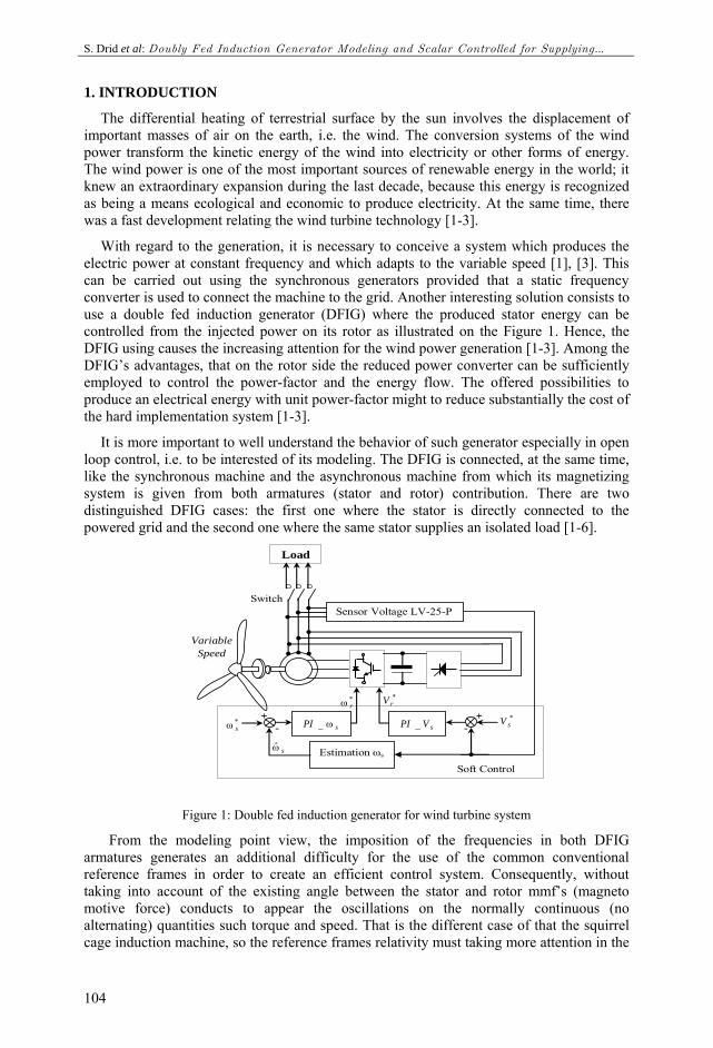
With regard to the generation, it is necessary to conceive a system which produces the electric power at constant frequency and which adapts to the variable speed [1], [3]. This can be carried out using the synchronous generators provided that a static frequency converter is used to connect the machine to the grid. Another interesting solution consists to use a double fed induction generator (DFIG) where the produced stator energy can be controlled from the injected power on its rotor as illustrated on the Figure 1. Hence, the DFIG using causes the increasing attention for the wind power generation [1-3]. Among the DFIG’s advantages, that on the rotor side the reduced power converter can be sufficiently employed to control the power-factor and the energy flow. The offered possibilities to produce an electrical energy with unit power-factor might to reduce substantially the cost of the hard implementation system [1-3].
It is more important to well understand the behavior of such generator especially in open loop control, i.e. to be interested of its modeling. The DFIG is connected, at the same time, like the synchronous machine and the asynchronous machine from which its magnetizing system is given from both armatures (stator and rotor) contribution. There are two distinguished DFIG cases: the first one where the stator is directly connected to the powered grid and the second one where the same stator supplies an isolated load [1-6].
Switch
Load
Variable Speed
sVPI _sPI ω_
Estimation ωs
+-
+ -
Sensor Voltage LV-25-P
*sV*
sω
sω
*rω
*rV
Soft Control
Figure 1: Double fed induction generator for wind turbine system
From the modeling point view, the imposition of the frequencies in both DFIG armatures generates an additional difficulty for the use of the common conventional reference frames in order to create an efficient control system. Consequently, without taking into account of the existing angle between the stator and rotor mmf’s (magneto motive force) conducts to appear the oscillations on the normally continuous (no alternating) quantities such torque and speed. That is the different case of that the squirrel cage induction machine, so the reference frames relativity must taking more attention in the
J. Electrical Systems 2-2 (2006): 103-115
105
DFIG system [7] and [9]. The previous angle is called torque angle, like in the synchronous machine, and of which it is necessary to take into account in the conventional Park transformations rotation in order to guarantee DFIG-system stability.
Thus this work is registered respecting to the DFIG space vector modeling with it’s the scalar using the separate reference frames. The experiment and digital simulation are carried out 0.8 kW laboratory machine will be shown an interesting results for future use of the DFIG-control-system on the serious wind powered region for supplying an isolated site on electric energy.
2. MACHINE MODELING
The voltage stator and rotor space vector equations, presented in complex notation, of an induction machine are given by the following system [7-9]:
( )( ) ( )
( )( ) ( )
sss s
s s s
rrr r
r r r
du R i
dtd
u R idt
φ
φ
⎧⎪⎪ = +⎪⎪⎪⎨⎪⎪⎪ = +⎪⎪⎩
(1)
Flux equations: ( ) ( ) ( )
( ) ( ) ( )
s s r js s s r
r r s jr r r s
L i M i e
L i M i e
θ
θ
φ
φ −
⎧⎪ = +⎪⎪⎨⎪ = +⎪⎪⎩ (2)
From (1) and (2), the model is written like ( ) ( )
( ) ( ) ( )
( ) ( )( ) ( ) ( )
. ( . )
. ( . )
s rs rs s j r
s s s s r
r sr sr r j s
r r r r s
di diu R i L M e j i
dt dtdi di
u R i L M e j idt dt
θ
θ
ω
ω−
= + + +
= + + − (3)
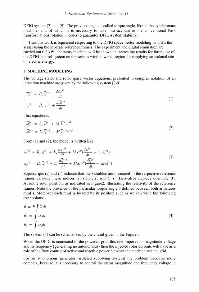
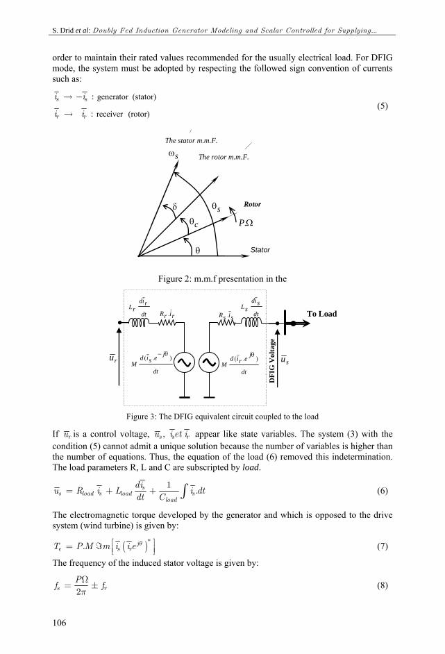
Superscripts (s) and (r) indicate that the variables are measured in the respective reference frames carrying these indices (s: stator, r: rotor). s : Derivative Laplace operator; :θ Absolute rotor position, as indicated in Figure2, illustrating the relativity of the reference frames. Note the presence of the particular torque angle δ defined between both armatures mmf’s. Moreover each mmf is located by its position such as we can write the following expressions:
c c
s s
P dt
dt
dt
θ
θ ω
θ ω
= Ω
=
=
∫∫∫
(4)
The system (1) can be schematized by the circuit given in the Figure 3.
When the DFIG is connected to the powered grid, this one imposes its magnitude voltage and its frequency (generating no autonomous) then the injected rotor currents will have as a role of the flow control of active and reactive power between the machine and the grid.
For an autonomous generator (isolated supplying system) the problem becomes more complex, because it is necessary to control the stator magnitude and frequency voltage in
S. Drid et al: Doubly Fed Induction Generator Modeling and Scalar Controlled for Supplying...
106
order to maintain their rated values recommended for the usually electrical load. For DFIG mode, the system must be adopted by respecting the followed sign convention of currents such as:
generator (stator)
receiver (rotor)
:
:
s s
r r
i i
i i
→ −
→ (5)
Stator
The stator m.m.F.
Rotor δ
θ
sθ
Ω.P cθ
sω The rotor m.m.F.
Figure 2: m.m.f presentation in the
su
sisR . dt
sidsL
dt
jeridM
).( θ
rirR .dt
ridrL
dt
jesidM
).( θ−
ru
DFI
G V
olta
ge
To Load
Figure 3: The DFIG equivalent circuit coupled to the load
If ru is a control voltage, ,s s ru i et i appear like state variables. The system (3) with the condition (5) cannot admit a unique solution because the number of variables is higher than the number of equations. Thus, the equation of the load (6) removed this indetermination. The load parameters R, L and C are subscripted by load.
1 .ss load s load s
load
diu R i L i dtdt C
= + + ∫ (6)
The electromagnetic torque developed by the generator and which is opposed to the drive system (wind turbine) is given by:
( )*. je s rT P M m i i e θ⎡ ⎤= ℑ ⎢ ⎥⎣ ⎦ (7)
The frequency of the induced stator voltage is given by:
2s rPf fπΩ= ± (8)
J. Electrical Systems 2-2 (2006): 103-115
107
The sign ± explains that the DFIG mmf’s rotations can be in the same or in the opposition direction.
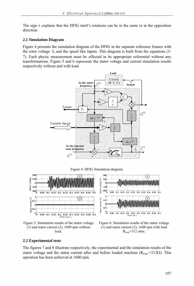
2.1 Simulation Diagram
Figure 4 presents the simulation diagram of the DFIG in the separate reference frames with the rotor voltage ru and the speed like inputs. This diagram is built from the equations (3-7). Each physic measurement must be effected in its appropriate referential without any transformations. Figure 5 and 6 represents the stator voltage and current simulation results respectively without and with load.
ri
θ
θ
−
+
)(ssi
)(ssu
)(rru
In the stator frequency
In the injected rotor frequency
dt
d
θjeM .
dt
dθ− jeM .
Tr
Rs
−
+
Load
Switch
P
)(rri
∑
dt
dLs
∫
Circuit (R_L_C)
Te
Variable Speed
Torque
Figure 4: DFIG Simulation diagram.
0 0.05 0.1 0.15 0.2 0.25 0.3 0.35 0.4 0.45 0.5-300 -150
0 150 300
Stat
or v
olta
ge
0 0.05 0.1 0.15 0.2 0.25 0.3 0.35 0.4 0.45 0.5-1
-0.5 0
0.5 1
Time (sec.)
Stat
or c
urre
nt (A
)
1
2
0 0.05 0.1 0.15 0.2 0.25 0.3 0.35 0.4 0.45 0.5 -300
--150
0
150
300
Stat
or v
olta
ge (V
)
0 0.05 0.1 0.15 0.2 0.25 0.3 0.35 0.4 0.45 0.5 -1
-0.5
0
0.5
1
Stat
or c
urre
nt (A
)
Time (sec.)
1
2
Figure 5: Simulation results of the stator voltage
(1) and stator current (2), 1600 rpm without load.
Figure 6: Simulation results of the stator voltage (1) and stator current (2), 1600 rpm with load
Rload=312 ohm.
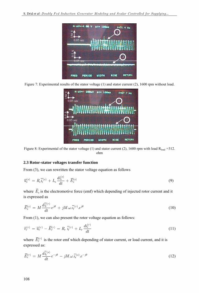
2.2 Experimental tests
The figures 7 and 8 illustrate respectively, the experimental and the simulation results of the stator voltage and the stator current after and before loaded machine (Rload =312Ω). This operation has been achieved at 1600 rpm.
S. Drid et al: Doubly Fed Induction Generator Modeling and Scalar Controlled for Supplying...
108
0.05 sec
150
V
0.05 sec
0.5
A
1
2
Figure 7: Experimental results of the stator voltage (1) and stator current (2), 1600 rpm without load.
2
1 0.05 sec
150
V
0.05 sec
0.5
A
Figure 8: Experimental of the stator voltage (1) and stator current (2), 1600 rpm with load Rload =312.
ohm
2.3 Rotor-stator voltages transfer function
From (3), we can rewritten the stator voltage equation as follows ( )
( ) ( ) ( )sss s s
s s s s sdiu R i L Edt
= + + (9)
where sE is the electromotive force (emf) which depending of injected rotor current and it is expressed as
( )( ) ( ). . .
rrs j r j
s rdiE M e jM i edt
θ θω= + (10)
From (1), we can also present the rotor voltage equation as follows: ( )
( ) ( ) ( ) ( )rrr r r r
r r r r r rdiv u E R i Ldt
= − = + (11)
where ( )rrE is the rotor emf which depending of stator current, or load current, and it is
expressed as: ( )
( ) ( ). . .ssr j s j
r sdiE M e jM i edt
θ θω− −= − (12)
J. Electrical Systems 2-2 (2006): 103-115
109
We consider that this rotor emf as a voltage disturbance because it depends of the stator current ( )s
si , varying with load, and rotor speed, varying with wind speed. So this rotor emf disturbance is considered such as the stator voltage must be maintained or regulated to its rated value. Consequently, the used control strategy must be designed in such manner that this considered disturbance is simply rejected.
Using (10) and (11), we can write the cause-effect transfer function between rotor and stator voltage as
( )
( )
( ) 1ss
ssr j
r rr
v
E M jR Tv e θ
ω⎛ ⎞ +⎟⎜= ⎟⎜ ⎟⎜⎝ ⎠ +s
s (13)
As mentioned above, the stator current must assumed too as disturbance, because the stator voltage must be maintained as constant for any electric load. So the regulation process conducts to realize that: ( ) ( ) ( )s s ss s sv u E= ≅ (14)
where ( ) ( ) ( )( )s s ss s s s sv u u i E= − Δ = (15)
with, ( )
( )( ) ( )
L
sss
s s s s s
D Disturbance Load
diu i R i Ldt
=
Δ = + (16)
With the previous assumptions, (13) becomes simply ( )
( )( )1
sss
r rr
v M jH s
R Tvω⎛ ⎞ +⎟⎜= = ⎟⎜ ⎟⎜⎝ ⎠ +
ss (17)
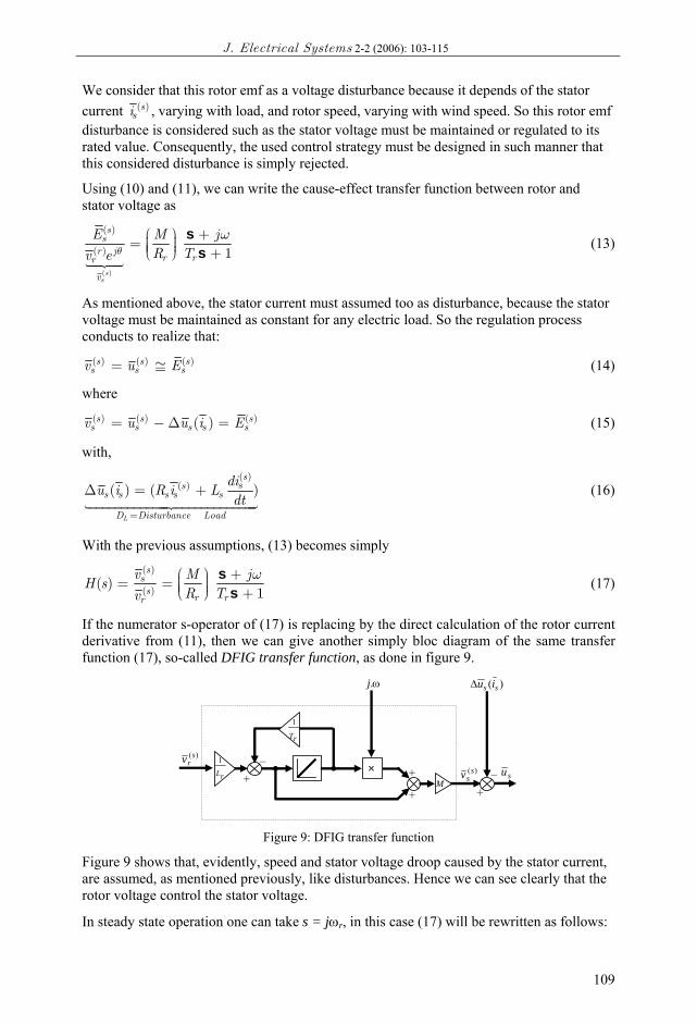
If the numerator s-operator of (17) is replacing by the direct calculation of the rotor current derivative from (11), then we can give another simply bloc diagram of the same transfer function (17), so-called DFIG transfer function, as done in figure 9.
ω.j )( ss iuΔ
− +
)(srv
)(ssv su − +
rL
1
rT
1
× +
+ M
Figure 9: DFIG transfer function
Figure 9 shows that, evidently, speed and stator voltage droop caused by the stator current, are assumed, as mentioned previously, like disturbances. Hence we can see clearly that the rotor voltage control the stator voltage.
In steady state operation one can take s = jωr, in this case (17) will be rewritten as follows:
S. Drid et al: Doubly Fed Induction Generator Modeling and Scalar Controlled for Supplying...
110
( )
( ) 1
ss ss
r r rr
v M jR j Tv
ωω
⎛ ⎞⎟⎜= ⎟⎜ ⎟⎜⎝ ⎠ + (18)
Where,
s rω ω ω= + (19)
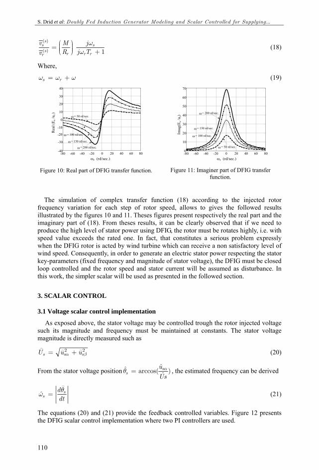
-80 -60 -40 -20 0 20 40 60 80-40 -30 -20 -10
0 10 20
30
40
ω = 200 rd/sec.
ω = 150 rd/sec.
ω = 100 rd/sec.
ω = 50 rd/sec.
Rea
l (E s
/ur )
ωr (rd/sec.) Figure 10: Real part of DFIG transfer function.
-80 -60 -40 -20 0 20 40 60 800
10
20
30
40
50
60
70
ω = 50 rd/sec.
ω = 100 rd/sec.
ω = 150 rd/sec.
ω = 200 rd/sec.
ωr (rd/sec.)
Imag
(Es /
u r)
Figure 11: Imaginer part of DFIG transfer
function.
The simulation of complex transfer function (18) according to the injected rotor frequency variation for each step of rotor speed, allows to gives the followed results illustrated by the figures 10 and 11. Theses figures present respectively the real part and the imaginary part of (18). From theses results, it can be clearly observed that if we need to produce the high level of stator power using DFIG, the rotor must be rotates highly, i.e. with speed value exceeds the rated one. In fact, that constitutes a serious problem expressly when the DFIG rotor is acted by wind turbine which can receive a non satisfactory level of wind speed. Consequently, in order to generate an electric stator power respecting the stator key-parameters (fixed frequency and magnitude of stator voltage), the DFIG must be closed loop controlled and the rotor speed and stator current will be assumed as disturbance. In this work, the simpler scalar will be used as presented in the followed section.
3. SCALAR CONTROL
3.1 Voltage scalar control implementation
As exposed above, the stator voltage may be controlled trough the rotor injected voltage such its magnitude and frequency must be maintained at constants. The stator voltage magnitude is directly measured such as
2 2s s sU u uα β= + (20)
From the stator voltage position ˆˆ arccos( )ˆs
suUs
αθ = , the estimated frequency can be derived
ˆ ss
ddtθω = (21)
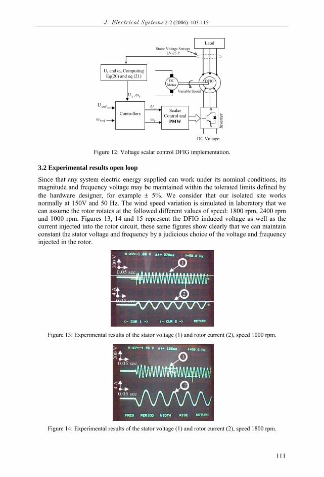
The equations (20) and (21) provide the feedback controlled variables. Figure 12 presents the DFIG scalar control implementation where two PI controllers are used.
J. Electrical Systems 2-2 (2006): 103-115
111
srefω rω
rUsrefU
Laod
DFIG
Inve
rter
Controllers
Us and ωs Computing Eq(20) and eq (21)
ssU ω,
Stator Voltage Sensors LV-25 P
Variable Speed
Scalar Control and
PMW
DC Motor
DC Voltage Figure 12: Voltage scalar control DFIG implementation.
3.2 Experimental results open loop
Since that any system electric energy supplied can work under its nominal conditions, its magnitude and frequency voltage may be maintained within the tolerated limits defined by the hardware designer, for example ± 5%. We consider that our isolated site works normally at 150V and 50 Hz. The wind speed variation is simulated in laboratory that we can assume the rotor rotates at the followed different values of speed: 1800 rpm, 2400 rpm and 1000 rpm. Figures 13, 14 and 15 represent the DFIG induced voltage as well as the current injected into the rotor circuit, these same figures show clearly that we can maintain constant the stator voltage and frequency by a judicious choice of the voltage and frequency injected in the rotor.
0.05 sec
200
V
0.05 sec
4 A
1
2
Figure 13: Experimental results of the stator voltage (1) and rotor current (2), speed 1000 rpm.
0.05 sec
200
V
0.05 sec
4 A
1
2
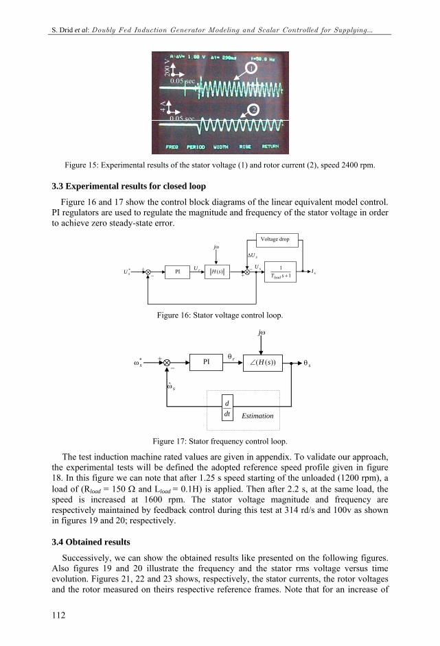
Figure 14: Experimental results of the stator voltage (1) and rotor current (2), speed 1800 rpm.
S. Drid et al: Doubly Fed Induction Generator Modeling and Scalar Controlled for Supplying...
112
0.05 sec
200
V
0.05 sec
4 A
1
2
Figure 15: Experimental results of the stator voltage (1) and rotor current (2), speed 2400 rpm.
3.3 Experimental results for closed loop
Figure 16 and 17 show the control block diagrams of the linear equivalent model control. PI regulators are used to regulate the magnitude and frequency of the stator voltage in order to achieve zero steady-state error.
PI )(sH 1
1+sTload
Voltage drop
+ −
− +
*sU sI
sUΔ
sU
ωj
rU
Figure 16: Stator voltage control loop.
PI ))(( sH∠+ −
*sω sθ
ωj
dtd
Estimation
sω
rθ
Figure 17: Stator frequency control loop.
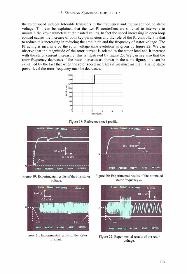
The test induction machine rated values are given in appendix. To validate our approach, the experimental tests will be defined the adopted reference speed profile given in figure 18. In this figure we can note that after 1.25 s speed starting of the unloaded (1200 rpm), a load of (Rload = 150 Ω and Lload = 0.1H) is applied. Then after 2.2 s, at the same load, the speed is increased at 1600 rpm. The stator voltage magnitude and frequency are respectively maintained by feedback control during this test at 314 rd/s and 100v as shown in figures 19 and 20; respectively.
3.4 Obtained results
Successively, we can show the obtained results like presented on the following figures. Also figures 19 and 20 illustrate the frequency and the stator rms voltage versus time evolution. Figures 21, 22 and 23 shows, respectively, the stator currents, the rotor voltages and the rotor measured on theirs respective reference frames. Note that for an increase of
J. Electrical Systems 2-2 (2006): 103-115
113
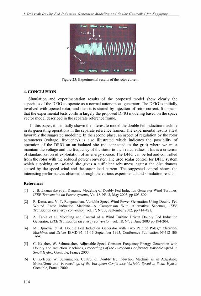
the rotor speed induces tolerable transients in the frequency and the magnitude of stator voltage. This can be explained that the two PI controllers are solicited to intervene to maintain the key-parameters at their rated values. In fact the speed increasing in open loop control causes the increase of both key-parameters and the role of the PI controllers is that to reduce this increasing in reducing the amplitude and the frequency of stator voltage. The PI acting is incarnate by the rotor voltage time evolution as given by figure 22. We can observe that the magnitude of the rotor current is related to the stator load and it increase with the stator current increasing; this is illustrated by figure 23. We can see also that the rotor frequency decreases if the rotor increases as shown in the same figure, this can be explained by the fact that when the rotor speed increases if we must maintain a same stator power level the rotor frequency must be decreases.
0 1 2 3 4 50
200
400
600
800
1000
1200
1400
1600
Time (sec.)
Spee
d (
rpm
)
Figure 18: Reference speed profile.
20 V/ div
0.5 s/ div
0
0 sec.
Figure 19: Experimental results of the rms stator
voltage.
100 (rd/s)/ div
0.5 s/ div 0
0 s
Figure 20: Experimental results of the estimated
stator frequency ωs
1 A/ div
0.2 s/ div
1 s 3 s
0
Figure 21: Experimental results of the stator
current.
10 V/ div
0.5 s/ div
0
0 sec.
Figure 22: Experimental results of the rotor
voltage.
S. Drid et al: Doubly Fed Induction Generator Modeling and Scalar Controlled for Supplying...
114
4 A/ div
0.5 s/ div
0
0 sec.
Figure 23: Experimental results of the rotor current.
4. CONCLUSION
Simulation and experimentation results of the proposed model show clearly the capacities of the DFIG to operate as a normal autonomous generator. The DFIG is initially involved with opened rotor, and then it is started by injection of rotor current. It appears that the experimental tests confirm largely the proposed DFIG modeling based on the space vector model described in the separate reference frame.
In this paper, it is initially shown the interest to model the double fed induction machine in its generating operations in the separate reference frames. The experimental results attest favorably the suggested modeling. In the second place, an aspect of regulation by the rotor parameters (voltage, frequency) is also illustrated which indicates the possibility of operation of the DFIG on an isolated site (no connected to the grid) where we must maintain the voltage and the frequency of the stator to their rated values. This is a criterion of standardization of exploitation of an energy source. The DFIG can be fed and controlled from the rotor with the reduced power converter. The used scalar control for DFIG system which supplying an isolated site gives a sufficient robustness against the disturbances caused by the speed wind and the stator load current. The suggested control shows the interesting performances obtained through the various experimental and simulation results.
References [1] J. B. Ekanayake et al, Dynamic Modeling of Doubly Fed Induction Generator Wind Turbines,
IEEE Transaction on Power systems, Vol.18, N°. 2, May 2003, pp 803-809.
[2] R. Datta. and V. T. Ranganathan, Variable-Speed Wind Power Generation Using Doubly Fed Wound Rotor Induction Machine—A Comparison With Alternative Schemes, IEEE Transaction on energy conversion, vol.17, N°. 3, September 2002, pp 414-421.
[3] A. Tapia et al, Modeling and Control of a Wind Turbine Driven Doubly Fed Induction Generator, IEEE Transaction on energy conversion, vol. 18, N°. 2, June 2003 pp 194-204.
[4] M. Djurovic et al, Double Fed Induction Generator with Two Pair of Poles,” Electrical Machines and Drives IEMD’95, 11-13 September 1995, Conference Publication N°412 IEE 1995.
[5] C. Keleber, W. Schumacher, Adjustable Speed Constant Frequency Energy Generation with Doubly Fed Induction Machines, Proceedings of the European Conference Variable Speed in Small Hydro, Grenoble, France 2000.
[6] C. Keleber, W. Schumacher, Control of Doubly fed induction Machine as an Adjustable Motor/Generator, Proceedings of the European Conference Variable Speed in Small Hydro, Grenoble, France 2000.

J. Electrical Systems 2-2 (2006): 103-115
115
[7] S. Drid, M-S. Nait-Said, M. Tadjine, The Doubly Fed Induction Machine Modeling In The Separate Reference Frames, Journal of Electrical Engineering, JEE. Vol.4, N°1, 2004, pp: 11-16.
[8] W. Leonhard, Control Electrical Drives, Springer verlag Berlin Heidelberg 1985. Printed in Germany.
[9] S. Drid, M-S. Nait-Said, M. Tadjine, “The Doubly Fed Induction Generator Modeling in the Separate Reference Frames for an Exploitation in an Isolated Site with Wind Turbine,” Third IEEE International Conference on Systems, Signals & Devices SSD'05, March 21-24, 2005, Sousse - Tunisia
Appendix
Rated Data of the Induction motor with wound rotor • Rated values: 0.8 kW ; 220/380 V-50 Hz ; 3.8/2.2 A
• Rotor-star connected: 3×120 V; 4.1 A ; 1420 rpm