Double-Shift High Schools and School Performance: Evidence from a Regression Discontinuity Design

Carlos Martín Muñoz Pedroza

1

Abstract

Policymakersindevelopingcountriesoftenresorttodouble‐shiftschoolingsystemsinordertomaximizeschoolingsupplyundertightbudgetconstraints.Thereishoweversome concern that this strategy trades off equality in school quality for costeffectiveness.Inthispaperweinvestigatewhetherornotthisisthecase.Inordertoovercometheselectionproblemsintheassignmenttothedifferentshifts,weexploitthediscontinuityintheassignmentofstudentstotheafternoonshiftgiventheirmiddleschoolGPA.UsingdatafromadministrativerecordsandasocioeconomicsurveyinahighschoolsysteminMexicoCity,wefindthatbeingassignedtotheafternoonshiftleadstoa12percentagepointsincreaseintheprobabilityofdroppingoutforfemalestudents,anda12.4percentagepointsdecreaseinthisprobabilityformalestudents.Wethenexploreonthemechanismsbehindthisasymmetricresponse,andconcludethatwomenaremorenegativelyaffectedbyworsepeersthanmen,menrespondmorepositively tohavingmorehomogenousgroups,andmenrespondmorepositively totheirrelativerankingintheirclassthanwomen.

Keywords:Drop‐outrates;highschool;double‐shiftschools;RDD;schooling;Mexico.

JELCodes:I20,I21,I24,I28,O54.

2

1. Introduction

Developingcountriesfaceseriousbudgetconstraintsthathindertheirabilitytoexpand

the education supply. As a result, policymakers have often resorted to double‐shift

schools(DSS)toincreasethesupplyofschoolspaces:theschoolopensforamorning‐

shift andanafternoon‐shift effectivelydoubling the amountof spaces available in a

schoolwithouttheneedtobuildadditionalinfrastructure.Thereare,however,some

drawbacks to double‐shift schools. It is argued that the afternoon‐shifts have lower

quality professors and lower quality students due to negative self‐selection. In

consequence, students attending the afternoon shift may have lower school

performancevis‐à‐visthestudentsinthemorningshift.Ananalysisofthecausaleffect

of the double‐shifts on school performance is difficult precisely because of this

selection. In this paper,we aim to overcome this estimation challenge by using the

exogenousassignmentrule(basedonmiddleschoolgradepointaverage)ofstudents

to the morning and afternoon shifts in Mexican high schools, which allows us to

implementaregressiondiscontinuitydesign.

TheMexicanMinistryofEducationbeganusingmultiple‐shiftsduringthesixties

asawaytoexpandschoolingsupply.1Currently, thedouble‐shiftsareawidespread

practiceinpublicschoolsatallschooling levels.Atthehighschool level,Mexicohas

achieved100%coverageofthestudentsapplyingtohighschool.However,thedropout

ratesinhighschoolarestillveryhigh:only62percentoftheenteringclassfinisheshigh

school.Inadditiontothis,ifonelooksatthedropoutratesinthemorningandafternoon

shift,onefindsastarkdifference.Inthemorningshift75percentofstudentsareable

to complete high school,whereas in the afternoon shift only 36 percentmanage to

completehighschool.2Thisdifferenceinhighschoolcompletionbetweenshiftsledus

toaskourselves if,despite itscost‐effectiveness, the implementationof themultiple

1Eventhoughwewillbetalkingaboutdoubleshifts(amorningandanafternoonshift),somepublicschoolsinMexicoofferthreedifferentshifts:morning,afternoonandnightshifts.Thenightshiftsaremostlyusedbyadults.2ThesefigurescomefromadministrativerecordsfromtheSchoolofSciencesandHumanities(CCHforitsSpanishacronym)whichareahighschoolsystempertainingtotheNationalAutonomousUniversityof Mexico (UNAM for its Spanish acronym). The Ministry of Education does not have statisticsdisaggregatedbyshiftsatthenationallevel.

3

shifts is leading to inequality of opportunities between students. Specifically, is the

afternoon shift hindering the opportunities of students to have access to schooling

quality, or is this just the effect of negative selection in the distribution of students

acrossshifts?

ThepossibilitythattheDSSpreventsomestudentstofinishhighschoolcould

have major economic effects. Zimmerman (2014) uses a regression discontinuity

design(RDD)toshowthatthegaininincomeassociatedwithadmissiontouniversity

ofamarginalstudentishigh.Studentsjustabovethecutoffgradeofhighschoolearn

anaverageof$1,593permonthmorethanthosewhoarejustbelow,thisrepresentsa

considerableefficiencygain.Theseimplicationscouldbegeneralizedtothecaseofhigh

schoolstudentswhocouldsee their future truncatedwhen theyareassignedto the

afternoonshift,andthislosscouldevenexceedthesavingsgeneratedbytheuseofDSS.

Inhisanalysis,Bray(2000)highlightsthatthemainbenefitofadoptingDSSis

thereductionoftheunitaryeducationcost.Thisismainlyachievedbecauseofthree

factors:amoreefficientuseofeducational infrastructure,even ifmaintenancecosts

increase;amoreefficientuseofhumancapitalbecauseprofessorsmaybeallowedto

teachinbothshifts;andareductionintheeffectiveeducationtimeforprofessorsand

students that can be invested in other activities, which is due to the reduction of

availableclassroomtime.Incontrast,somepotentialcostsarisingfromtheadoptionof

DSSare:1)thenecessitytohirechildcareservicesforworkingparents,2)thenecessity

ofadditionaltutoringtocompensatethereductionsonclassroomtime,and3)social

problemsarisingfromthebaduseofstudents’leisuretime.

The figureson schooldesertion support the commonbelief that themorning

shiftis“better”thantheafternoonshiftamongparentsandstudents.Infact,parents

strive to get their children enrolled in morning shift instead of the afternoon one.

However,thereisnoevidencetosupportthesebeliefs;thatis,thattheafternoonshift

isinherentlyoflowerquality(Linden,2001).Peoplejustifythisprioronthebasisthat

the afternoon shift receives the worst students, but there is no consensus among

researchersthatthisisactuallytrue.Infact,thereisveryscantliteratureontheimpact

ofthiseducationpolicy,andmostoftheevidencedoesnothaveacausalinterpretation.

4

Theschoolprincipalstendtofirstallocatestudentstothemorningshift,andoncethe

spacesareexhaustedinthisshifttheybeginenrollingstudentsintheafternoonshift.

Ingeneral,principalsdonotfollowauniformcriteriaintheallocationofstudentstothe

differentshifts.Notwithstanding,students’characteristicsineachshiftdiffermakingit

verydifficult toestimate the causal effectof thispolicy. Inhis study,Linden (2001)

compared one‐shift schools vis‐à‐vis double‐shift schools in OECD countries, and

concludesthatthelatterschoolsofferanadequateeducationandcouldbeusedasa

convenienteducationalpolicy.

Cardenas (2011)carriedoutanextensivereviewof the literatureonDSS.He

summarizesitinthreegeneralpoints:first,hefindslittleempiricalevidenceaboutthe

differences in performance between shifts; second, he concludes that principals,

teachersandstudentsfacedifferentchallengesineveryturn;andfinally,hesaysthat

previousresearchhasidentifiedasegregationsystemthatassignsstudentsbasedon

their socioeconomic profile (Saucedo‐Ramos, 2005). He also shows that, when

comparingbothshifts,onaveragetherearemorepoorstudents,lowerperformanceon

standardizedtests,aswellashigherdropoutandfailureratesintheafternoonshift.

Neitherauthoriscapabletogiveacausalargument,sincetheiridentificationstrategy

cannotcontroltheselectionproblemsintheallocationofshift.

Sagyndykova(2013)studiestheeffectofDSSinMexicanelementaryschoolsand

concludesthatDSSisanappropriatesolutionforcountrieswithlimitedbudgets.She

applies the Heckman selection model to measure the effects of observable

characteristicsonstudentperformance,andfindsapositiveeffectforbeingassignedto

themorningshift.However,the"OaxacaDecomposition"showsthatthiseffectcanbe

explainedbyobservablecharacteristicsofthestudent,schoolandteachers.Herresults

show that the self‐selection of students explains the apparent achievement gap

betweenstudentsfromdifferentshifts.

Inthispaper,weaimtodetermineifDSS,whichhashelpedtoprovideuniversal

accesstoschoolinginMexico, leadstoareductioninschoolquality intheafternoon

shift. Inparticular,weare interestedonwhether theobserveddifferences in school

performancebetweenthemorningandafternoonshiftsarecausal.Tothiseffect,we

5

willuseseveralmeasuresofperformance,butourmainfocuswillbeondropoutrates.

Inordertoidentifythecausaleffectoftheafternoonshiftonschoolperformancewe

willexploittherulesofassignmentinasystemofUNAM’shighschoolsknownforits

acronym, CCH (School of Sciences and Humanities). CCH’s assign students to the

morningandafternoonshiftsbasedontheirmiddleschoolgradepointaverage(GPA).

Dependingonthequalityoftheenteringclass,theadministrativeauthoritiesinCCH

determineathresholdlevel,8.5(outof10)inmostcases,sothatstudentsbelowthis

threshold are assigned to the afternoon shift. This assignment rule allows us to

implementafuzzyregressiondiscontinuitydesign(RDD)toidentifytheeffectofbeing

allocated to theafternoonshift, so thatwepurgeourestimatesof thenegativeself‐

selection that usually plagues this kind of analysis (Van der Klaauw, 2002). To our

knowledge,thisisthefirstpaperthatstudiestheeffectofmultipleshiftsusinganRDD.

This assignment rulemay generate differentmechanisms throughwhich the

school performance of a studentmaybe affected. For instance, the assignment rule

amountstoatrackingsystemusesstudents’academicabilitytoseparatethestudents

intothetwoshiftssothateachshiftisrelativelymorehomogenousinitscomposition

(Hidalgo‐Hidalgo,2011).Trackingsystemshavetwopotentialeffects.Ontheonehand,

itallowsprofessorstotargettheirteachingleveltothemeanofthegroupbydecreasing

theabilitygapbetweenthemostablestudentandtheleastablestudent.Ontheother

hand, theremaybeapeereffectwithineachshift:highabilitystudentsmaybenefit

morefromtheirinteractionwithotherhighabilitystudents,andlowabilitystudents

maydecreasetheirperformanceevenfurtherwheninteractingwithotherlowability

students.Thislattereffectwouldincreaseinequalityinperformancebetweenthetwo

shifts.

BettsandShkolnik(1999)concludethatdespitetheemergingconsensusthat

high‐achieving students arebenefited in tracking schools and that lowperformance

studentsareaffected,thisconsensusisbasedoninvalidcomparisons.Whencomparing

similarstudentstheyconcludethattheeffectonlow‐performancestudentsisnulland

that high‐performance students improve. More recently, Duflo, Dupas and Kremer

(2011)conductedanexperimentinKenyainwhichtheyexamineddifferencesbetween

6

schoolswithandwithouttrackingandalsoanalyzedtheimpactforstudentsindifferent

partsoftheperformancedistribution.Theyfindevidencethatseparationintogroups

byperformancepositivelyaffectsacademicperformanceforeveryone.

Anothermechanismthatwewill investigateistherelativerankingeffect.The

assignmentrulechangestheincentivesofstudentswhobarelymadeittothemorning

shiftandthosewhobarelymissedthemorningshift.Thefirstgroupofstudentshave

thelowestrank,basedontheirmiddleschoolGPA,intheirclass‐shift.Thesecondgroup

ofstudents,thosewhobarelymissedthemorningshift,havethehighestrankinthe

class‐shift. These relative rankings may change the subjective perception that the

studentshaveabouttheirownability,suchthatanincreaseintherelativerankingmay

induce them to exert more effort and thus improve their school performance.

WeinhardtandMurphy(2014)measurethelongtermimpactoftheordinalrankingof

studentsinanelementaryschool.Theyshowthattohaveahighrankingamongpeers

hasagreatpositiveeffectonyourlong‐termacademicperformance.

IftheeffectofDSSdependsonthesetwomechanisms,aswehypothesize,then

theoveralleffectisamatterofempiricalanalysis.Ifpeereffectsaremoreimportant,

thenwewouldexpectstudentsintheafternoonshiftofdecreasetheirperformance.If

trackingworksinfavorofallstudentsasinDuflo,DupasandKremer(2011),theeffect

oftheafternoonshiftwilldependontherelativesizeoftheincreasesinperformance.

Finally,ifrelativerankingmatters,wewouldexpectstudentswhobarelymissedthe

morningshift,andarethusintheafternoonshift,toincreasetheirperformancerelative

tostudentswhobarelymadeitintotheafternoonshift.

Inourestimates,weuseddatafromadministrativerecordsoftheCCHs,allof

them located inMexicoCity, and a socioeconomic survey collected at enrollment in

everyCCH.Inthedataweareabletoidentifyeachstudentduringthetimesheremains

enrolled in a CCH, so the data has a longitudinal structure.We have data for eight

differententeringclassesbetween2005and2014.Theserecordshavedataongrades,

highschoolcompletion,admissiontoUNAM,campusofenrollment,class,shift,gender,

andmanyothervariables.EachCCHhasapproximately3,600studentsperentering

class.

7

Wefindthatthereareheterogenouseffectsoftheafternoonshiftonthedropout

ratesofmenandwomen,andothergroupsofinterest.Inthecaseofmen,beinginthe

morning shift decreases de probability of dropping out by 12.4 percentage points,

whereas for women we find an increase in the probability of dropping out of 12

percentagepoints.Ourexplorationofthemechanismsbehindthesechangessuggests

thattheeffectonmenismostlydrivenbychangesintherelativeranking,whereasthe

change in women is mostly driven by negative peer effects. We also find that the

studentswhoworkarethemostbenefitedbytheirassignmenttotheafternoonshift:

theirprobabilityofdroppingoutdecreasesby14.7percentagepoints.

Inaddition,wefindthatwomenintheafternoonshifthaveahigherprobability

ofchoosingascience, technology,engineeringormathematics(STEM)major (an11

percentage point increase), whereas this probability decreases by 19.4 percentage

pointsformalestudents.Wealsofindthattheprobabilityofbeingadmittedtoamajor

in high demand at UNAM decreases by 14.3 percentage points for women, but it

increasesby17.1percentagepointsformen.Wesuggestthatthesegenderdifferences

inmajorselectionarearesultofachangeinthegendercompositionofeachshift.

Ourmaincontributioninthispaperisourabilitytomeasurethecausaleffectof

the afternoon shifts in DSS on school performance. Our identification strategy

eliminates theselectionproblemthatpreviousresearchhasnotbeenable to tackle,

even ifweareonlyable to identifya local average treatment effect. Inaddition,we

provideevidenceofgenderdifferencestonegativeincentives,peereffectsandattitudes

towardscompetitioninanon‐laboratorysetting.Finally,weprovidesomesuggestive

evidencethatthecompositionofthegroup(i.e.proportionofmenandwomeninthe

group)affectsmajorpreferencesofindividuals.

Therestofthepaperisorganizedasfollows.Section2describestheresearch

design. In this sectionwe describe the identification strategy, the data used in our

estimationsandsomebackgroundaboutCCHs inorder tounderstand thesourceof

identification.Section3presentsthemainresults.Section4presentsadiscussionof

ourresultsandconcludesthepaper.

8

2. Researchdesign

In this section we will explain our research design. We will first present the

identificationstrategy,thenthedatathatwewillusetoproduceourestimates,andwe

willalsogivesomebackgroundaboutCCHsinMexicoCity.

2.1. Identificationstrategy

Ourobjectiveistoestimatethecausaleffectofbeingassignedtotheafternoonshifton

school performance. If the assignment were randomized, we could estimate the

followingequation:

(1)

wheretheoutcomevariable isequalto1ifthestudentdroppedoutofschooland

equalto0ifshesuccessfullyconcludedhighschool; isequalto1ifthestudent

wasassignedtotheafternoonshiftandequalto0ifshewasassignedtothemorning

shift;and isarandomerror.Inthiscase,theparametermeasuringtheeffectwould

be .

However, as inmost of applied research, the afternoon shift is not randomly

assigned;thatis,thereissomeformofselectionintothedifferentshifts.Thisselection

inducesabiasontheestimatorof ,sincetherewouldbesomedependencebetween

and .Hence, | 0andbecauseoftheendogeneityof ,theOLS

estimatorwillbeinconsistentandlackcausalinterpretation.Inourcontext,weobserve

thatstudentswithhigherperformanceareassignedtothemorningshiftandtherestto

theafternoonshift.There isaclearselectionproblem.Asaresult, theprobabilityof

droppingoutinthemorningshiftcouldbedifferentfromtheprobabilityintheevening

shift;however, this isnotnecessarily theeffectofbeing intheafternoonshift,buta

confoundedeffectofshift,andstudentsobservedandunobservedcharacteristic(such

as,theirability).

9

In order to eliminate the selection bias, we exploit the assignment rule of

students to the afternoon shift. After talking to the administrative staff of CCHs, it

becameveryclear tous that theassignmentrulewasrelated tomiddleschoolGPA:

those students with a GPA higher than a cutoff had a greater probability of being

assigned to the morning shift. Hence, the assignment methodology creates a

discontinuityintheprobabilityoftreatment.Thissuggeststhatthetreatmenteffectcan

beconsistentlyestimatedusingafuzzyregressiondiscontinuitydesign(RDD)(Imbens

andLemieux,2008).Theintuitionbehindthisapproachisthatstudentswhoarejust

abovethecut‐offpointareverysimilarinobservableandunobservablecharacteristics

tothosejustbelowit.Thisallowsustocomparetheresultsshownbystudentswhoare

near the threshold. The identification strategy is based on the assumption that all

characteristicsthataffectthestudent’sresults,buttheprobabilityofassignmenttothe

afternoon shift, change smoothly over the threshold. As a result, any change in the

outcomevariablecanbesolelyattributedtoenrollmentintheafternoonshift.

The fuzzyRDD can be estimated using instrumental variables as long as the

orderofthesmoothingpolynomialandtheestimationbandwidthusedforthefirstand

forthesecondstagesarethesame(VanDerKlaauw,2002).Thefirstandthesecond

stagesinthiscaseare:

(2)

(3)

where istheoutcomevariableofinteresttothestudent ,fromcampus andclass ;

isanindicatorequalto1ifthestudentisassignedtotheafternoonshiftand

equalto0ifsheisassignedtothemorningshift; isacharacteristic

functionindicatingwhetherthestudent’smiddleschoolGPA( isbelowthe

cutoff of campus and class ; is a vector of the student’s observable

characteristics; and arefixedeffectsforcampusandclass,respectively; and

are random error terms. Finally, is the polynomial control for the

regression discontinuity. is still the parameter of interest, which, under the

identification assumptions, constitutes a local average treatment effect. That is, the

10

effectcorrespondstothosestudentswhowouldbeassignedtotheafternoonshift if

theyhadhadanaveragesecondarygradebelowthecut‐off,butwouldbeassignedto

themorningiftheyhadhadanaveragesecondarygradeoverthecut‐off.

Inordertodeterminethedegreeofthesmoothingpolynomial ,we

willusetheAkaikeinformationcriterion.Wewillestimatetheequationsaboveusinga

bandwidth around the cutoff, which will be determined following Imbens and

Kalyanaraman(2008).Forrobustness,wewillalsousedifferentbandwidthsaround

the cutoff grade.Theaim is to restrict the sample and to compare similar students,

identifyingtheaforementionedlocalaveragetreatmenteffect.Finally,sincethemiddle

schoolGPA inourdatabase is rounded toonedecimalpoint, thedistributionof the

runningvariableisdiscrete.Standarderrorsare,thus,clusteredatmiddleschoolGPA

levelasrecommendedbyLeeandCard(2008).

2.2. Data

ThedatacomesfromasystemofhighschoolsadministeredbyUNAM,theColegiode

CienciasyHumanidades(CCH),whichconsistsof5campuses:Naucalpan,Azcapotzalco,

Vallejo,East,andSouth.Eachenteringclasshas3,600studentsdividedbetweenthe

morningandafternoonshifts.Ourdatabasecomesfromtwosources:administrative

data provided by the General Directorate of CCH, and data from a socioeconomic

questionnaireappliedbytheDirectorateGeneralofPlanningandEvaluationatUNAM.3

Thesampleiscomposedofobservationsatthestudentlevelandcoveringeightclasses

inaperiodfrom2005to2014.Forthepurposeofthisanalysis,allcampusesandclasses

havebeencombinedintoasinglesample.

The administrative database contains information on the academic record of

eachstudentenrolledintheCCHduringtheperiodofanalysis.IthasmiddleschoolGPA,

highschoolGPApersemester,numberofapprovedcourses,admissiontoUNAM,and

information on school desertion, school expulsion or graduation. This database is

3ThedatawasrequestedthroughthetransparencyofficeofUNAM,No.applicationF10897.

11

complementedbyasocioeconomicquestionnaire,whichincludesinformationonthe

personal and family characteristics of the student such as: type of middle school

(public/private), shift inmiddle school, age, gender, academic habits and attitudes,

parents’ schooling level, student employment status, and household income, among

others.

Therestrictedsampleconsistsofstudentsbetween14and16yearsold,where

15yearsoldistheregularentryage.4Welimitourdatatothisagerangebecausewe

presumethatstudentsover16yearsofageareunderdifferentcircumstanceswhich

mayleadtoabiasinourresults.Thefinalsampleincluded73%oftheoriginalsample,

that is, 96,794 students. Four campuses of the 2007 generationdo not have all the

required informationandwereexcluded from thedataset.Given theRDdesign, the

sampleislimitedtostudentswithinabandwidthof0.40GPApointsaroundthecutoff.5

Restricting the sample to observations around the threshold leaves uswith 31,372

students.

Table1showsdescriptivestatisticsbyshift.PanelApresentsinformationfor

theentiresample.Inthemorningshift61%ofstudentsarewomen,averageentryage

is15.15years,averagemiddleschoolGPAis9.11,and11%ofthestudentswork.When

we compare the statisticsof themorning shiftwith thoseof theafternoon shift,we

observedstatisticallysignificantdifferencesinthepercentageofwomen(44%inthe

afternoonshift)and inaveragemiddleschoolGPA(7.91 intheafternoonshift).The

significantdifferencesinthosevariablessuggestthatgenderandmiddleschoolGPAare

correlated with shift assignment. Although all the differences are statistically

significant,themagnitudeofthedifferenceintherestofthevariablesdoesnotseem

economicallysignificant.

4About10%ofthosewhowereadmittedwere16yearsoldatentry.5TheoptimalbandwidthwasdeterminedfollowingImbensandKalyanaraman(2011).

12

2.3. AdmissionandshiftassignmentinCCHs

Theadmissionprocessfortheentirepublichighschoolsysteminthemetropolitanarea

of Mexico City is rare and is done on an annual basis. The process is led by the

Metropolitan Commission of Public Institutions for Higher Secondary Education

(COMIPEMS for its Spanish acronym). Admission is determined based on the score

obtainedonthestandardizedadmissiontestandonthepreferencesoftheapplicant

overtheparticipatinginstitutions.TheCOMIPEMSthendetermineswhichstudentsare

admitted toeachpublichighschool inMexicoCity.TheCCHshaveacceptancerates

rangingfrom22%to48%.6

Once the student is admitted to a CCH, it is assigned to one of two shifts.

AccordingtotheguidetoadmissiontotheUNAMhighschoolsystem, theallocation

processisrandom;thatis,assignmenttotheafternoonshiftdoesnotdependonthe

middle school GPA, gender or age, nor any other characteristic of the student. The

allocationisonlysupposedtobalancethenumberofstudentspergroup.However,a

detailedanalysisofthedatashowsthattheallocationofshiftisconditionalatleaston

threeobservablestudentcharacteristics:themiddleschoolGPA,genderandage,with

theGPAalmostfullydeterminingtheshift.

Assignmenttotheafternoonshiftalsodependsonthecharacteristicsofstudents

beingadmittedeachyear.Inparticular,thecutoffvalueofmiddleschoolGPAmaybe

differentforeachgender,campusandenteringclassbecauseitdependsonthenumber

ofapplicantsandthedistributionofthemiddleschoolGPAofthoseaccepted.Also,the

assignmentrulegivesprioritytowomen,whichmaycausetheexistenceofdifferent

cutoff points for men and women. The minimum average grade necessary to be

assigned to the morning shift is not known in any case. These differences in the

thresholdoftheassignmentrulearetakenintoaccountinourRDDestimation.Since

thecutoffforeachcampus‐class‐genderisnotknown,wefirstestimatethecutoffvalues

usingthemethodologyproposedbyCard,MasandRothstein(2008)andalsousedby

6Basedondatafromtheenteringclassof2013,inwhich55,190applicantscompetedfor18,000availablespaces.

13

Ozier(2011).Oncewehavethecutoffvaluesforeachclassandcampus,were‐center

therunningvariablearoundeachcutoffatthegender‐campus‐classlevel.

The identification of the cutoff values or discontinuity points is based on

structuralchangeanalysis(Cardetal.,2008).Thefirststepistoestimatearegression

of the treatment variable (afternoon shift) against a hypothetical discontinuity

indicator,whichrangesfrom7.0to10.0inincrementsofone‐tenthcontrollingfora

flexible polynomial of the running variable (middle school GPA). This procedure is

performedindependentlyforeachclass,campusandgender.Foreachcombinationof

class,campusandgender,therealpointofdiscontinuity(cut‐offpoint)istheonewhose

regressionproducesthehighestR‐squared.

IngeneralwefindthatthepointsofdiscontinuityareataGPAof8.5(outof10)

formenandwomen.However,insomeyearswomenshowsomecutoffpointsataGPA

of8.9.Assupplementaryevidence,thesameprocedureisappliedtothewholesample,

separatingonlybetweenmenandwomen.Theresultshowsthatthecutoffpointisa

GPAof8.5formenandwomen.TheresultisshowninFigure1.

Aswementionedabove,sincethecutoffpointsvarybygender‐class‐campus,we

re‐centeredtherunningvariableinsteadofusingtheactualvalueofthemiddleschool

GPA.Thereare twoalternatives for re‐centering theGPA: (1) re‐center the running

variableusingthecutoffat8.5forallstudents,assuggestedbythestructuralchange

analysis for the whole sample; or (2) re‐center the running variable using the

correspondingcutoffpointappliedtoeachstudent,accordingtohergender,classand

campus. Figure 2 shows graphically the cutoff point and thediscontinuity for both

alternatives.Asarobustnesstest,weusebothalternativeinourestimatesofthecausal

effectoftheafternoonshift,buttheresultsareshownonlyforthesecondalternative.7

PanelBofTable1presentsthedescriptivestatisticsforthediscontinuitysampleusing

thesecondre‐centeringalternativewithabandwidthof0.40pointsaroundthecutoff.

7Theresultsarerobusttobothre‐centeringalternatives.

14

3. Empiricalresults

3.1. TestingfortheidentificationassumptionsoftheRDD

Inordertogiveacausal interpretationtoourestimates, theRDDmustsatisfysome

identificationassumptions.Themainconcernisthatassignmenttotheafternoonshift

aroundthethresholdisnotasifitwererandomized;thatis,thatsomehowstudents

know the treatment assignment rule and they are able tomanipulate theirmiddle

schoolGPAinordertobeassignedtothemorningshift,which isarguablythemost

desirable.

Manipulationofthetreatmentassignmentrulecouldhappenifstudentscould

convincetheir teacherstochangetheirmiddleschoolGPAor if theycould finetune

theireffortinordertogetaGPArightabovethecutoffGPAinordertobeadmittedto

themorningshift.Inouropinion,itisverydifficulttomanipulatethisGPAinorderto

barely get into themorning shift. This ismostly duebecause of the following three

reasons.First,middleschoolGPAdependsontheeffortexertedinschoolduringthree

years.Itisobtainedbytakingtheaverageof30differentcourses,manyofthosetaught

bydifferentteachers.SofinetuningtheGPAsuchthatitisrightabove8.5seemslikea

very unlikely event. Second, as wementioned in the previous section the guide to

admission to UNAM’s high schools falsely claims that assignment to the shifts is

randomized.Hence,studentsarguablydonotknowthetreatmentassignmentrule.And

finally,evenifstudentshaveanideathattheyneedacertainGPAtogetenrolledinthe

morningshift,wefoundthatthecutoffmayvary,thuscreatinguncertaintyonthevalue

ofthecutoffforeachgender‐campus‐classcombination.Asaresult,sortingaroundthe

thresholdmaybeunlikely.

If there were self‐selection around the cutoff, we would expect to find a

discontinuityinthedistributionofmiddleschoolGPAaroundthethresholdrequiredto

beenrolledinthemorningshift;thatis,adisproportionatenumberofstudentswould

sortthemselvesintobeingrightabovethecutoffascomparedtothoserightbelowthe

15

cutoff. Figure 3 shows the distribution of middle school GPA. We do not see any

clusteringofobservationsrightabovethecutoff.Inaddition,weperformedMcCrary’s

(2008)densitytesttoformalizethisnotion.8Wefoundthatthediscontinuityaround

the threshold is not statistically significant, and thus we conclude that there is no

manipulation of the running variable in ourRDdesign.9Another possible source of

selection of the studentswould be if observationswithmissing values are selected

around the threshold. Figure 4 shows the percentage of observationswithmissing

valuesovertherangeoftherunningvariable,andwedonotobserveanydiscontinuity

atthecutoffeither.

AnotheralternativetotestthevalidityoftheRDDistoexamineiftheobservable

characteristicsofthestudentsarecontinuousaroundthethreshold.Figure5presents

the graphical evidence on this assumption for age, gender, admission test score,

student’s employment status, and parents’ schooling level. We do not observe any

discontinuitiesinthesevariables.

ThelasttwocolumnsofPanelBinTable1showthedifferenceofthemeansof

themorningandtheafternoonshift,andthep‐valueofat‐testtocheckwhetherthe

differenceisstatisticallysignificantaroundthethreshold.Weobservesmalldifferences

aroundthethresholdandtheyareallstatisticallysignificant.However,wedonotthink

that any of these differences are big enough in magnitude to be considered

economicallyrelevant,especiallygiventhelargeamountofobservations.Forinstance,

the7percentdifferenceinthenumberofwomenbetweenthemorningshiftandthe

afternoonshiftamountstohaving126additionalwomeninthemorningshiftforeach

class‐campusonaverage.Forthesereasons,wewillconcludethatthetreatmentand

control groups are relatively comparable. In any case, we will also control for

observable characteristics in our estimations, and we will also do estimations for

8Inessence,McCrary’stestisatestofthecontinuityoftherunningvariabledensityfunction.Thetestisanextensionoflocallinearregressionwithestimatesofasmootheddensityoftherunningvariablemadeseparatelyonbothsidesofthethreshold.Astatisticallysignificantdifferenceintheinterceptsofbothregressionswouldimplythatthereisadiscontinuityintherunningvariableatthethreshold.Thetestisvalid only ifmanipulation ismonotonic; that is, studentsmanipulate their GPA only to get into themorningshift,butnottogetintotheafternoonshift.9Theestimateddiscontinuityisequalto‐0.0023withastandarderrorof0.0155.

16

subgroups of the population (women,men, and by employment status), whichwill

makethetreatmentandcontrolgroupsevenmorecomparable.

3.2. First‐stage:discontinuityintheprobabilityoftreatment

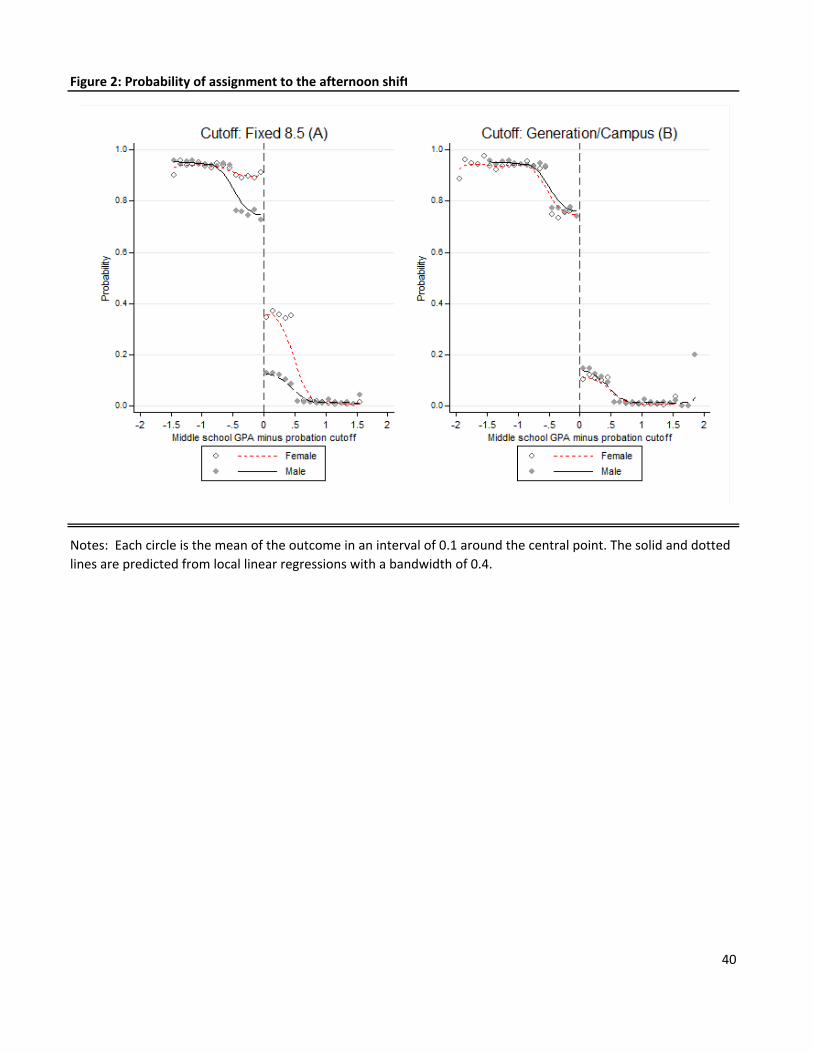
InFigure2weshowedthatthereisadiscontinuityintheprobabilityofbeingassigned

totheafternoonshift.Recallwewillbere‐centeringtherunningvariableusingallthe

estimatedcutofflevelsatthegender‐campus‐classlevel.Inthegraphthemagnitudeof

thediscontinuityisofabout0.6,whichmeansthatstudentswithascorerightbelow

the cutoff decrease the probability of being enrolled in the morning shift by 60

percentage points. Table 2 formalizes this graphical analysis by estimating the first

stageinequation(2).Columns1to3presenttheresultsusingthewholesample,the

nextthreecolumnsusethesampleofwomen,andthelastthreecolumns,thesampleof

men. We report the estimates without and with the smoothing polynomial on the

runningvariable.10Wechoseathird‐degreepolynomialwithdifferentslopesoneither

sideofthethresholdusingtheAkaikecriterion.11Inaddition,wealsocontrolforage,

gender,parents’yearsofschooling,student’semploymentstatus,dummiesofwhether

thestudenthaschildrenorismarried,andcharacteristicsofhermiddleschool(such

aswhetheritwaspublicorprivate,andtheshiftinwhichshewasenrolled).Wealso

controlledforfixedeffectsatthecampusandclasslevel.

The estimated discontinuity is robust to the different specifications and

subsamples. In our least parsimonious specification, we found that having a score

below the cutoff increases the probability of being in the afternoon shift by 61.6

percentagepoints(pp)forthewholesample,by66.1ppforwomen,andby55.2ppfor

men.The fact that the estimatorswith andwithout controls are very similar in the

10Recallthispolynomialiscrucialintheidentificationstrategy.11 In fact thispolynomial specification is thebest fit even fordifferentvaluesof thebandwidth.TestresultsofrobustnesswithdifferentorderpolynomialsandbandwidthsareshowninTable1ofAppendixA.

17

differentsamplessupportsourconclusionthatthetreatmentandcontrolgroupsare

indeedquitecomparablearoundthethreshold.

3.3. EffectsofafternoonshiftonGPA

Table 3 reports the results on GPA of the first semester, GPA of the last semester,

percentagechangeintheGPAbetweenmiddleschoolandthefirstsemester,percentage

change in the GPA up to the last semester, probability of high school desertion,

probabilityof admission tomajors inhighdemandatUNAM, and theprobabilityof

choosingandbeingadmitted toaSTEMmajoratUNAM.Eachcoefficient inTable3

comes from a different regression of the outcome variable on the afternoon shift

dummyvariable;thatis,eachcoefficientisadifferentestimateof inequation(3).The

firstfourcolumnsofTable3presentfourdifferentspecificationsfortheestimatesusing

thewholesample:withoutandwiththesmoothingpolynomialonmiddleschoolGPA,

withstudent’scharacteristicsandbackgroundcontrols,andwith fixedeffectsat the

campus and class level. The least parsimonious specification controls for the third‐

degreepolynomial,student’scharacteristicsandbackground,campusfixedeffects,and

classfixedeffects.Henceforththiswillbeourpreferredspecificationandthisistheone

weusefortheestimationswiththedifferentsubsamplesincolumns5to8ofTable3.

Wewill firstdescribe the resultsof the impactof theafternoonshiftonhigh

school grades. Grades range from zero to ten points, with six being the minimum

passinggrade.HighschoolinCCHconsistsofsixsemesters.PanelAofTable3presents

theresultsfortheGPAofthefirstsemesterofhighschool.Whenusingthecomplete

sample,wecanseethattheresultsarerobusttotheinclusionofthedifferentcontrols

exceptforthethird‐degreesmoothingpolynomialwhichisnecessaryforidentification

inanRDD.WeestimatethattheeffectoftheafternoonshiftonfirstsemesterGPAis

between0.15and0.14points(outof10).Whenwelookatdifferentsubsamples,we

findthattheeffectsisslightlylargerformen(0.16points)thanforwomen(0.12points).

Wealsoobservethatbeingintheafternoonshiftbenefitsstudentswhoworkthemost:

theirgradesincreasebyalmost0.4pointsascomparedtostudentswhoworkwhoare

18

inthemorningshift.Studentswhodonotworkbenefittheleast,butstillobserveagain

inalmost0.1pointsascomparedtothoseinthemorningshift.12

PanelBofTable3presentstheresultsfortheGPAinthesixthsemester(thelast

oneofhighschool).Whenconsideringthewholesample,theresultsaresimilartothose

inthefirstsemesterwithaneffectoftheafternoonshiftofabout0.14to0.12pointsin

theGPA.However,thedifferencesbetweenmenandwomenbecomemoreacute.Inthe

lastsemesterofhighschool,menintheafternoonshiftexhibitanincreaseof0.25points

ascomparedtomeninthemorningshift;whereaswomenonlyincreasetheirgrades

by0.05points. Thedifferencesbetweenemployed andnon‐employed students also

widen:employedstudentsgainalmost0.6pointsfrombeingenrolledintheafternoon

shift,whereasthosenon‐employedonlygain0.05,ascomparedtothoseinthemorning

shift.

Whenanalyzinggrades,apossibleconcern is that teacherscurvegrades,and

thus change the distribution of grades for bothmorning and afternoon shifts. This

practicewouldrenderthegradesuselesstocompareperformanceacrossshifts.Figure

6presentsascatterplotofthemeanGPAinthefirstandlastsemesterswithrespectto

therunningvariable(there‐centeredmiddleschoolGPA).Ifteacherswerecurvingthe

grades,thenthebeststudentsineachshiftwouldget10orsomethingcloseto10(i.e.

anA+)andtherestwouldbeassignedagradethatcorrespondstotheirplaceinthe

distribution of grades. If this were true and grades in high school are positively

correlatedwithgradesinmiddleschool,inFigure6weshouldthenseetwoincreasing

lines on each side of the threshold which would be more or less parallel. The

discontinuityatthethresholdwouldthusbeverylarge(ofabout4pointsconsidering

thattheminimumpassinggradeis6).Sothediscontinuityingradesthatweestimate

maybeonlyanartifactduetocurvedgrades.Figure6showsthatthisisnotthecase.

Gradesareinfactincreasingoverthewholerangeoftherunningvariableimplyingthat

teachersarenotcurvingthegradeswithinshifts.Inaddition,thediscontinuityatthe

12Pleasekeepinmindthattheinterpretationofallourresultsareforthesamplearoundthecutoff;thatis,thoseobservationswithinthe+/‐0.4bandwidth.

19

thresholdissmallinmagnitude;asweexplained,withacurve,thediscontinuitywould

bemuchlarger.

Wenowturnourattentiontochangesingradesbetweenmiddleschoolandhigh

school.Figure7presentsthepercentagechangeofgradesinhighschool(firstandsixth

semesters)ascomparedtomiddleschoolGPA.Wefindthatallstudentsdecreasetheir

gradesbetweenmiddleschoolandhighschoolonaverage(therangeofthepercentage

changeinthey‐axisisalwaysnegative).Rosenkranzetal.(2014)explainthatthisdrop

ingradesisduetochangesinattendanceandeffortinthetransitionfrommiddleschool

tohighschool.Theyarguethatstudentsinhighschoolhavegreaterlibertiesandthus

perceiveattendanceandeffortasachoiceratherthananobligation.

Inadditiontoageneralizeddecreaseingrades,wealsoobservethatthestudents

withhighergradesinmiddleschoolexhibitthelargestdropingradesascomparedto

studentswithlowermiddleschoolgrades.Weobserveadiscontinuityatthethreshold

implyingthatthoseintheafternoonshiftdonotdroptheirgradesasmuchasthosein

themorningshift.PanelsCandDofTable3presenttheseresults.Forthewholesample,

we estimate an increase of about 1.3 pp and 1 pp for the first and last semesters,

respectively,onthepercentagechangeofgradeswithrespecttomiddleschoolGPA.

Again,menandemployedstudentsexhibitthelargestgainsfrombeingenrolledinthe

afternoonshiftascomparedtothoseinthemorningshiftaroundthethresholdlevel.

Thegenderdifferences,andworkingstatusdifferencesalsowidenbetweenthe first

andlastsemester,asexpected.

Insum,wefindthatstudentsintheafternoonshiftdisplayahigherperformance,

asmeasured by grades, than students in themorning shift around the cutoff value.

Althoughallstudentsdroptheirgradesinhighschool,studentsintheafternoonshift

droptheirgradesbylessthanstudentsinthemorningshift.Wepresentedevidence

thatthisisnotduetothecurvingofgrades(whichmaybethemostobviousdifference

inacademicstandards).Itmaybeduetoadifferenceinmonitoringofstudents,maybe

teachersconsiderthatstudentsintheafternoonshiftareabitmoreproblematicand

thus monitor them more strictly. But we cannot offer any evidence on this latter

hypothesis.

20

3.4. Outcome:Highschooldesertion

The outcome of greatest interest to us is high school desertion. This is a more

straightforwardmeasureofhighschoolperformance that isnotsubject to thesame

criticisms as grades. According to the Organization of Economic Cooperation and

Development(OECD,2013),inMexicomorethan40percentofstudentsbetween15

and19yearsoldarenotenrolledin(high)school.Partofthispercentageisduetothe

studentsdroppingoutoftheeducationsystembeforeenrollingtohighschool.Ofthose

whoenrollinhighschool,15percentdecidetodropoutnationwide(ascomparedto7

percent in the US). CCH desertion rates are much larger; as we mentioned in the

introduction,38percentofCCHstudentsdropout.

Figure8showstheimpactoftheafternoonshiftondrop‐outratesforthewhole

sample.Thereisnodiscernibleeffectofassignmenttotheafternoonshiftondrop‐out

rates, but this result ismasking some interesting facts. Figure 9 presents the same

graph,butdividedbysubgroupsofthepopulation:women,men,employedandnon‐

employed. In this figure,we can identify twogroupswhosedrop‐out rates increase

whentheyareenrolledintheafternoonshift:womenandnon‐employedstudents.In

contrast,menandemployed studentsdecrease their chancesof droppingoutwhen

theyareenrolledintheafternoonshift.

Panel E of Table 3 presents the formal estimates of those effects. Using the

complete sample,we find that studentswhoare justbelow thecutoffhaveahigher

probabilityofdroppingoutthanstudentsjustabovethecutoffof2.1pp(Column4).

For women, however, the increase in drop‐out rates is of 12 pp and for men the

decreaseindrop‐outratesis12.4pp.Employedstudentsalsodecreasetheirprobability

ofdesertingby14.7pp,whereasnon‐employedstudentsincreasetheirprobabilityby

4.9pp.

The fact that employed students are the oneswho gain themost frombeing

enrolledintheafternoonmakesintuitivesense.Workingandstudyingmaybemore

compatiblewhenstudentsareenrolledintheafternoonshift,thanwhenthestudents

areinthemorningshift.However,thegenderdifferencesinperformanceattributedto

21

theshiftarenotasintuitive.Maleandfemalestudentsaretaughtthesamecoursesand

bythesameteachers.Unless,teacherstreatthemdifferently,thenwewouldnotexpect

toobservethesedifferencesapriori.Wecannotprovideanyevidenceonhowteachers

treattheirstudents,sincethisisunobservabletous.Wewilllookintootherhypothesis

inordertoexplainthesegenderdifferences.

Our findings so far contradict the common belief that parents have: the

afternoonshiftisworsethanthemorningshift.Wehavefoundthat,inacomparableset

ofstudents,studentsintheafternoonshifthavehighergrades,droptheirhighschool

grades by less as compared tomiddle school, andmen have lower desertion rates,

althoughwomenhavehigherdrop‐outrates.Whyisthisthecase?Wehavetwomain

hypothesis:atrackingeffectandarelativerankingeffect.

The treatment assignment rule in our case is almost analogous to a tracking

system: thebeststudentsare left in themorningshift,while theworststudentsare

enrolledintheafternoonshiftonthebasisofthemiddleschoolGPA.AccordingtoDuflo,

Dupas and Kremer (2011), tracking has two different effects. First, splitting the

studentsinthisfashionmakesthegroupsmorehomogenoussothatteacherscanfocus

theiracademicleveltotheaveragestudent.Sincethegroupsaremorehomogenous,

thedistancebetweenthebestandworststudentsandtheaveragestudentislower,and

thuseveryonecanbebenefitedfrommorehomogenousclasses.Ifthiseffectdominates,

performancewouldbehigherinboththemorningandafternoonshift,sotherelative

effectisunknown.Thesecondeffectoftrackingreferstopeereffects.Giventhatthe

beststudentsarealllefttogether,theywillbenefitfrombeingincontactwiththebest.

Incontrast,theworststudentsarelefttogetherandtheir“bad”behaviormayevenget

worse when surrounded by “bad apples”. If this effect dominates, students in the

morningshiftwouldhavebetterperformancerelativetostudentsintheafternoonshift.

Inourdesignwedonotobserveachangefromtheregularsystemtoatracking

system.However,wecanexploitthevariationinthecutoffvaluestoshedsomelighton

theeffectofhavingmorehomogenousgroups.Alowervalueofthecutoffwouldimply

thattheafternoonshiftbecomesmorehomogenousrelativetothemorningshift,and

thusperformanceintheafternoonshiftshouldincreaserelativetothemorningshift.

22

Therewouldalsobealargernegativepeereffectintheafternoonbecausetherewould

beeven less “goodapples”.Thus,witha lowervalueof thecutoff: if thehomogeneity

effectdominates,weshouldobservethattheafternoonshifthasbetterperformancethan

themorningone.Incontrast,ahighervalueofthecutoffwouldimplythattheafternoon

shiftismoreheterogenousrelativetothemorningshift,andhenceperformanceinthe

afternoonshouldfallrelativetothemorning.Thenegativepeereffectsintheafternoon

arenowattenuatedbyadmittingmore“goodapples”.Then,withahighervalueofthe

cutoff:iftheheterogeneityeffectdominatesthepeereffect,thenweshouldobservethat

theafternoonshiftperformsworsethanthemorningshift.

Recall that thecutoffvaluevariesat thegender‐campus‐class level.Usingthe

structuralchangeanalysis,wefoundtwodifferentcutoffvaluesforwomen:8.4and8.9;

and twodifferent cutoffvalues formen:7.9and8.4.Table4presents the resultsof

estimatingtheeffectoftheafternoonshiftondesertionseparatelyforeachcutoffvalue.

Wefindthatanincreaseinthevalueofthecutoffforwomenleadstoanincreaseinthe

performanceoftheafternoonshift:womenadmittedtotheafternoonshiftwithan8.9

cutoffhavealowerdesertionratethanwomenadmittedtotheafternoonshiftwithan

8.4 cutoff. Hencewe can conclude that in the case ofwomen the peer effect is the

dominantone.Incontrast,menwithalowercutoffratedecreasetheirdesertionrates

evenmore,andthusthehomogeneityeffectdominatesinthecaseofmen.

Another interpretation of our results could be that being assigned to the

afternoonshiftrepresentsanegativeincentiveforthestudent,sincethemorningshift

ismoredesirable.Ourresultscontributetotheliteratureongenderdifferencesinthe

responsetoincentives,wherepreviousresearchfindsthatwomenaremoreresponsive

topositiveincentivesthanmen(Lindo,SandersyOreopoulos,2010).Inthispaper,we

find that men respond with a higher performance (a lower desertion rate) to the

negative incentive (afternoon shift), whereas women respond with a lower

performance(higherdesertionrate)tothesamenegativeincentive.

Itisalsoimportanttonoticethatevenwhenbothmenandwomenfacethesame

cutoff,thesignoftheafternoonshifteffectondesertionisdifferentacrossgenders.This

iswherewethinkthesecondmechanismisimportant,therelativerankingeffect.The

23

literatureongenderdifferencesinthepreferencesforcompetitionmayshedsomelight

onthegendergapthatwefind.AccordingtotheexperimentsconductedbyGneezy,

Niederle and Rustichini (2003), and Niederle and Vesterlund (2007), when the

environmentismorecompetitive,menincreasetheirperformance,butwomendonot,

especially if women have to compete against men. This gender difference in the

attitudes towards competition may explain the gender gap in performance in the

afternoonshift.

The assignment rule to the afternoon shiftmechanically changes the relative

ranking that the students havewith respect to their peers. Say the cutoff is 8.5 for

everyone,sothatastudentwith8.5isassignedtothemorning,butastudentwith8.4

isassignedtotheafternoon.AstudentwhohasaGPAof8.4isrankedinthemiddleof

thewholedistributionofstudents,justbelowsomeonewithan8.5,andbothstudents

wereaveragestudentsintheirrespectivemiddleschools.Butifweapplythetreatment

ruleofassignment,thestudentwithan8.5issuddenlyamongtheworstofthemorning

shift,andthestudentwithan8.4isamongthebestoftheafternoonshift.Thesechanges

intherelativerankingsofbothstudentsmayhaveapsychologicaleffectinthestudent.

MurphyandWeinhardt(2014)claimthatself‐confidencemaybethemechanismthat

betterexplainstheirfindingsontheimpactofordinalrankingonschoolperformance.

Other mechanisms could be competitiveness, self‐assessments of ability, or an

environmentthatfavorscertainranks(i.e.teachingdirectedtothetopoftheclass).

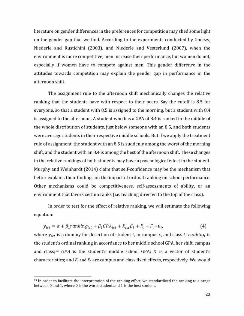
Inordertotestfortheeffectofrelativeranking,wewillestimatethefollowing

equation:

, (4)

where isadummyfordesertionofstudent ,incampus ,andclass ; is

thestudent’sordinalrankinginaccordancetohermiddleschoolGPA,hershift,campus

and class;13 is the student’s middle school GPA; is a vector of student’s

characteristics;and and arecampusandclassfixedeffects,respectively.Wewould

13Inordertofacilitatetheinterpretationoftherankingeffect,westandardizedtherankingtoarangebetween0and1,where0istheworststudentand1isthebeststudent.

24

thusexpect 0;thatis,beingbetterrankedamongtheirpeers,leadsthestudentsto

alowerdesertionrate.

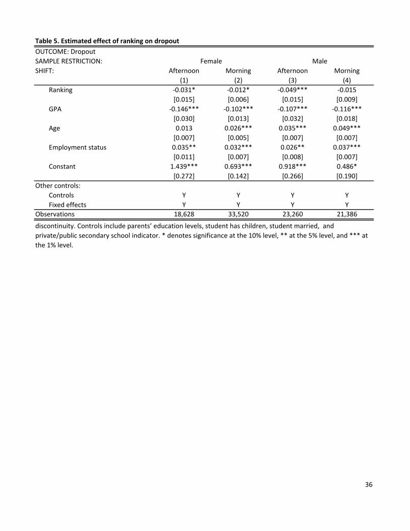
WepresenttheresultsoftheestimatesinTable5.Ingeneralweobservethat

both men and women in all shifts benefit from being better ranked. However, the

estimatesfromtheafternoonshiftare larger inmagnitudethantheestimatesof the

morningshift.Furthermore,menexhibitaneffectofranking58percenthigherthan

womenintheafternoonshift,butnotinthemorningshift.Recallthatthebeststudents

inthemorningshiftdonotreallyseeachangeintheirrelativerankascomparedtohow

they did in middle school. However, the best students in the afternoon shift do

experienceachangeintheirordinalrank.Wethinkthatthisrelativechangeandthe

subsequent boost in their motivation (self‐assessment or self‐confidence) may be

drivingtheseresults.

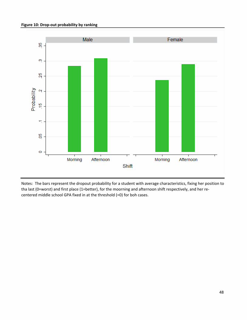
Figure 10 shows the predicted desertion probability for students at the

thresholdusingtheestimatesfromequation(4);thatis,wesettheordinalrankingto1

forafternoonstudents,and0formorningstudents,there‐centeredmiddleschoolGPA

issetatzero(thecutoff),andallothercharacteristicsareevaluatedatthemeanofthe

sample. Our objective here is to see if the relative ranking effect helps explain the

treatmenteffectondesertion.Onceweconsiderranking, thedifference indesertion

ratesbetweentheafternoonandthemorningshiftisnowpositiveformenandequalto

2.6 pp, and forwomen this differences is of 5.2 pp. This suggests thatmost of the

estimated effect of the afternoon shift for men is due to a relative ranking effect.

However, women do not respond as much to the relative ranking. This gender

difference in the response to relative ranking is in accordance to Murphy and

Weinhart’s(2014)findings.

3.5. Collegeadmission(UNAM)

The students who successfully complete high school at CCH earn their right to be

admitted toUNAM for college. This implies that theydonot participate in the very

competitive admission process that students from non‐UNAM high schools have to

25

undergo.However,admissiontocertainhighdemandmajorsisnotguaranteed,sinceit

dependsonhighschoolperformance.

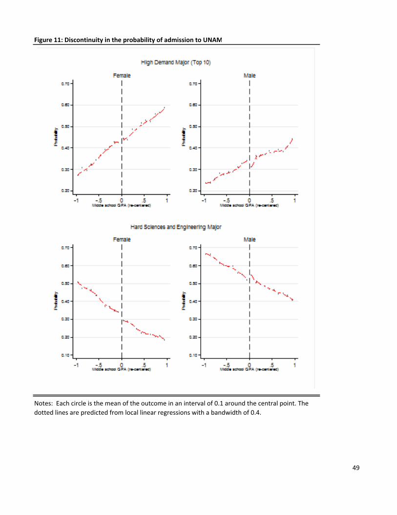
PanelF inTable3presents theeffectof afternoonshifton theprobabilityof

being admitted to a high demandmajor at UNAM (top 10).14Whenwe look at the

complete sample, we find that the afternoon shift leads to a drop of 2.2 pp in the

probability of being admitted to a high demand major. This result again masks

important differences between men and women: whereas women exhibit a lower

probabilityofbeingadmittedtooneofthosemajors(by14.3pp),menpresentahigher

probabilityofadmission(by17.1pp)ascomparedtostudentsinthemorningshift.This

effect is in accordancewith previous results sincewe have found thatmen at have

higheracademicperformancewhencomparedtomeninthemorning;hence,theyare

betterenabledtobeingacceptedtoamorecompetitivemajor.Finally,PanelGinTable

3reportstheeffectontheprobabilityofbeingadmittedtoSTEMmajorsatUNAM.We

findthatfortheoverallsample,theeffectoftheafternoonshiftonthisprobabilityis

negative,implyingadropin1.1pp.However,wefindthatwomenintheafternoonshift

increasetheirchancesofbeingacceptedtoaSTEMmajorby11pp,whilemendecrease

their chances by 19.4 pp as compared to students in the morning shift. Figure 11

presentsthegraphicalrepresentationoftheseresults.

How canwe explain these gender differences in the acceptance rates to the

differenttypesofmajors?InTable6wepresentthepercentageofwomenadmittedto

thetop10majorsindemand(PanelA)andtotheSTEMmajors(B).Weseethatahigh

percentageofwomenareadmittedtohighdemandmajors(63percent),whereasalow

percentageof39percentareadmittedtoSTEMmajors.Razo(2008)describesSTEM

majors as typicallymasculine. The author argues that one of themany factors that

influencewomenintheirmajorchoiceistheopinionoftheirpeers,besidestheopinion

of family members and personal preferences. Only 39 percent of students in the

morningshiftaremen,whereas56percentofstudentsaremenintheafternoonshift.

14 We consider the major with higher demand in 2011, which were: law, medicine, psychology,architecture, dentistry, communication sciences, biology, management, accountancy, and veterinary.Thesehighdemandmajorschangelittleovertime.

26

SoitispossiblethathavingmoremalepeersissteeringmorewomenintoSTEMmajors

thanintothehighdemandmajorswhichseemtobefemale‐dominated.Ourresultson

desertionsuggestedthat females in theafternoonshiftaremore influencedbytheir

peers.Thisinfluencemaygobeyondanegativeeffectondesertionrates,andintothe

collegemajorchoice.

4. Discussionandconclusions

Thereissomeconcernthat,eventhoughdouble‐shiftschooling(DSS)systemsarean

effectiveway to increaseeducation supply at lowcost, they couldbe increasing the

inequalityofopportunitiesacrossstudents in themorningandafternoonshifts. It is

wellknownthattheworststudentstendtobeenrolledintheafternoonshift,thusDSS

systemsmaywidenthegapbetweenthestudentsinbothshifts.Knowingtheeffectof

DSSonstudents’performanceisthusveryimportanttoassesstheoverallcostsofDSS

systems.However, it is very difficult to estimate the effect of being assigned to the

afternoonshiftonschoolingperformancepreciselybecauseofthosenegativeselection

ofstudents.

Inthispaper,wesolveforthisestimationchallengebyexploitingtheassignment

ruletotheafternoonshiftimplementedintheCCHsystemofUNAM’shighschools.The

assignmentrulesinducestudentswithahighGPAinmiddleschooltobeassignedto

themorningshiftwithahigherprobability.TheassignmentruleusesacutoffGPAthat

variesbygender,campus,andclassdependingonthecharacteristicsofeachincoming

class.Wethususethisassignmentruletoimplementafuzzyregressiondiscontinuity

design.

Our results do not support the common beliefs that the afternoon shift is

intrinsicallyworse.Wefindthatstudentsintheafternoonshifthavebettergradesthan

studentsinthemorningshiftaroundthecutoff.Thegainsingradesarelargerformen

thanforwomen,andforemployedstudentsthanfornon‐employedstudents.Wealso

provideevidenceforothermeasuresofperformancesuchasdesertion,andadmission

27

todifferent subsetsofUNAMmajors. In theseothervariables theresultswereeven

moreinterestingbecausewefoundlargeandopposingeffectsformenandwomen.

Women in the afternoon shift desert school with a higher probability than

women in themorning shift;whereasmen desert less than theirmale peers in the

morningshift.Weadvancetwomechanismsonwhythismaybethecase:atracking

effectandarelativerankingeffect.First,thetrackingeffectresultsfromsplittingthe

studentson thebasisofmiddle schoolGPA.The trackingeffect is composedof two

opposingrelativeeffects:theeffectofhavingamorehomogenousgroupthatfacilitates

teachingtothemean,andthepeereffect.Wefindthatmentendtobenefitfromhaving

morehomogenousgroups in theafternoonshift, butwomenarenegativelyaffected

fromhavingworsepeersintheafternoonshift.

Thesecondmechanismthatwetestistherelativerankingeffect.Theassignment

rule to the afternoon shift automatically changes the relative ranking of students

aroundthethresholdlevel.Thoserightabovethethresholdendupinthemorningshift,

buttheyaretheworstamongtheirpeers;while,thoserightbelowthethresholdend

upintheafternoonshift,buttheyarethebestamongtheirpeers.Thesechangesinthe

relativerankingmaychangetheself‐imageofstudents,theself‐confidenceortheself‐

assessment of their capabilities. Whichever the case, research has found that men

respondmoretoordinalrankingthanwomen(MurphyandWeinhart,2014),andwe

confirmthoseresultsinthispaper.Mendecreasetheirdesertionratesmorewhenthey

arerankedrelativelyhigher,andespeciallyiftheyareintheafternoonshift.Although

womenalsorespondpositivelytoranking,wedonotfindlargedifferencesacrossshifts,

whichiswhatreallymattersinourresearchdesign.Westillneedtodofurtherresearch

topinpointtheunderlyingmechanismbehindourresults.

Finally,welookedintotheeffectofbeingenrolledintheafternoononadmission

todifferentsubsetsofmajorsatUNAM,whereCCHstudentswhosuccessfullycomplete

highschoolhaveareservedspace.Weanalyzedtheeffectonbeingadmittedtothetop

tenmajorsindemand,whicharearguablythemostdifficulttogetinto.Wefoundyet

againadifferencebetweenmenandwomen:womenintheafternoonshifthavealower

chanceonbeingadmittedtoahighdemandmajor,whilemenhaveahigherchanceof

28

admission.Theseresultsareinaccordancetoourpreviousfindings.However,whenwe

lookatSTEMmajors,nowwomen in theafternoonshifthaveahigherchance tobe

admittedtoaSTEMmajorthanwomeninthemorningshift,andtheoppositeistrueof

men.Ifwomenaremoreinfluencedbytheirpeers,asourresultsondesertionsuggest,

then women in the afternoon shift, who have more male peers than those in the

morningshift,maychangetheirpreferencestowardsmoremasculinemajorssuchas

theSTEMmajors.

Given our results, our paper contributes to the literature on the impact of

education policies that use double‐ or multiple‐shift schooling in order to increase

schooling supply. Our results contrast with those in Sagyndykova (2013), but she

analyzes students in middle school who may still perceive their schooling as an

obligation. More interestingly, we also contribute to the literature on the gender

differencesintheresponsetoincentives,competition,andpeers.

Therearetwomaindrawbacksinouranalysis.First,wecouldnotgetdataon

thequalityofteacher,instructionaltime,andqualityofinstruction.WetalkedtoaCCH

teacherwhodeclared thatusually theafternoonshifthasexactly thesame teachers

thanthemorningshift.Ifanything,wewouldexpecttheteacherstobemoretiredin

theafternoonthaninthemorning,butthiswouldpointtoworsequalityofinstruction,

which is not consistentwith our results. The seconddrawback is that our research

designonlyallowsustoestimatealocalaveragetreatmenteffect(LATE).Wemaynot

beabletogeneralizeourconclusionstothoseindividualsoutsideofthebandwidththat

weusedinouranalysis.However,wedoresolvetheproblemofhavingatreatmentand

acontrolgroupwhicharecomparable,whichismuchmorethanpreviousliteraturehas

achieved.

29

References

Betts,J.R.andJ.L.Shkolnik(1999).“Keydifficultiesinidentifyingtheeffectsofability

groupingonstudentachievement”.EconomicsofEducationReview,19(1):21‐26.

Bray, M. (2000). Double‐shift schooling: Design and operation for cost‐effectiveness.

London:CommonwealthSecretariatUNESCO.

Card,D.,A.Masand J.Rothstein (2008). “Tippingand thedynamicsof segregation”.

QuarterlyJournalofEconomics,123(1):177‐218.

Cárdenas,S.(2011).“EscuelasdedobleturnoenMéxico:Unaestimacióndediferencias

asociadas con su implementación”. RevistaMexicana de Investigación Educativa,

16(50):801‐827.

Duflo, E., P. Dupas andM.Kremer (2011). “Peer effects, teacher incentives, and the

impact of tracking: Evidence from a randomized evaluation in Kenya”.American

EconomicReview,101(5):1739‐1774.

Gneezy, U., M. Niederle, and A. Rustichini (2003). “Performance in competitive

environments:Genderdifferences”.Quarterly JournalofEconomics,118(3):1049‐

1074.

Hidalgo‐Hidalgo,M.(2011).“Ontheoptimalallocationofstudentswhenpeereffects

areatwork:trackingvs.mixing”.SERIEs,2(1):31‐52.

Imbens,G.andK.Kalyanaraman(2011).“Optimalbandwidthchoicefortheregression

discontinuityestimator”.ReviewofEconomicStudies,79(3):933‐959.

Imbens, G. and T. Lemieux (2008). “Regression discontinuity designs: A guide to

practice”.JournalofEconometrics,142(2):615‐635.

Lee,D. S. andD.Card (2008). “Regressiondiscontinuity inferencewith specification

error”.JournalofEconometrics,142(2):655‐674.

30

Lindo,J.M.,N.J.Sanders,andP.Oreopoulos(2010).“Ability,gender,andperformance

standards:Evidencefromacademicprobation”.AmericanEconomicJournal:Applied

Economics,2(2):95‐117.

McCrary, J. (2008). “Manipulation of the running variable in the regression

discontinuitydesign:Adensitytest”.JournalofEconometrics,142(2):698‐714.

Murphy,R.andF.Weinhardt(2014).“Topoftheclass:Theimportanceofordinalrank”.

CESifoWorkingPaperNo.4815.

Niederle,M.andL.Vesterlund(2007).“Dowomenshyawayfromcompetition?Domen

competetoomuch?”.QuarterlyJournalofEconomics,122(3):1067‐1101.

OECD (2013). “Panorama de la educación 2013: México”. Nota país. Accessed on

January 20, 2016 at

http://www.oecd.org/edu/Mexico_EAG2013%20Country%20note%20(ESP).pdf.

Ozier, O. (2011). “The impact of secondary schooling in Kenya: A regression

discontinuityanalysis”.PhDDissertation,UniversityofCalifornia,Berkeley.

Razo,M.(2008).“Lainsercióndelasmujeresenlascarrerasdeingenieríaytecnología”.

PerfilesEducativos,30(121):63‐96.

Rosenkranz,T.,M.delaTorre,W.D.Stevens,andE.M.Allensworth(2014).Freetofail

oron‐trackcollege:Whygradesdropwhenstudentsenterhighschoolandwhatadults

candoaboutit.Chicago:ConsortiumonChicagoSchoolResearch.

Sagyndykova, G. (2013). “Academic performance in double‐shift schooling”. PhD

Dissertation,UniversityofArizona.

Saucedo‐Ramos, C. (2005). “Los alumnos de la tarde son los peores: prácticas y

discursosdeposicionamientode la identidaddealumnosproblemaen laescuela

secundaria”.RevistaMexicanadeInvestigaciónEducativa,10(26):641‐668.

Van der Klaauw,W. (2002). “Estimating the effect of financial aid offers on college

enrollment:A regressiondiscontinuity approach.” InternationalEconomicReview,

43(4):1249‐1287.

31

Zimmerman,S.D.(2014).“Thereturnstocollegeadmissionforacademicallymarginal

students”.JournalofLaborEconomics,32(4):711‐754.

Mean  S.D. Mean  S.D. Difference P‐value

Panel A. Full Sample

Characteristics

Female 0.61 0.49 0.44 0.50 0.17 0.000

Age 15.15 0.41 15.30 0.49 ‐0.14 0.000

Middle school GPA 9.11 0.51 7.91 0.51 1.20 0.000

Diagnostic entrance test 6.73 0.73 6.45 0.63 0.28 0.000

Employment status 0.11 0.31 0.17 0.37 ‐0.06 0.000

Years of schooling: Mother 10.57 3.54 10.78 3.48 ‐0.21 0.000

Years of schooling: Father 10.85 4.19 11.03 4.21 ‐0.18 0.000

Household income* 2.43 1.27 2.53 1.29 ‐0.10 0.000

Outcomes

High school GPA: 1st semester 8.06 1.01 7.17 1.07 0.88 0.000

High school GPA: Last semester 8.22 0.92 7.30 1.01 0.91 0.000

Admitted: Top 10 majors UNAM 0.46 0.50 0.29 0.45 0.17 0.000

Drop‐out rate 0.36 0.43 0.50 ‐0.27 0.00 0.000

Observations 54,906         41,888        96,794         

Panel B. Discontinuity Sample +/‐ 0.4

Characteristics

Female 0.59 0.49 0.52 0.50 0.07 0.000

Age 15.16 0.41 15.26 0.47 ‐0.10 0.000

Middle school GPA 8.73 0.30 8.39 0.26 0.34 0.000

Diagnostic entrance test 6.70 0.70 6.38 0.59 0.32 0.000

Employment status 0.12 0.32 0.15 0.35 ‐0.03 0.000

Years of schooling: Mother 10.81 3.51 10.56 3.47 0.25 0.000

Years of schooling: Father 11.06 4.22 10.90 4.14 0.16 0.000

Household income* 2.52 1.30 2.43 1.24 0.09 0.000

Outcomes

High school GPA: 1st semester 7.68 0.96 7.47 1.04 0.21 0.000

High school GPA: Last semester 7.87 0.88 7.61 0.98 0.26 0.000

Admitted: Top 10 majors UNAM 0.41 0.49 0.37 0.48 0.04 0.000

Drop‐out rate 0.22 0.41 0.32 0.47 ‐0.11 0.000

Observations 18,030 13,342 31,372

Notes: Panel B shows descriptive statistics restricting the full sample to 0.4 points arround the cutoff point of the 

assignation variable determined for each class/campus/gender.

*Definition of household income vairable is as follows: Categorical Variable = 1: 1‐2 minimum wages, 2: 3‐4 minimum 

wages, 3: 5‐6 minimum wages.

Table 1. Descriptive statistics

Morning shift Afternoon shift

Variable

32

OUTCOME: Afternoon Shift

SAMPLE RESTRICTION:

(1) (2) (3) (4) (5) (6) (7) (8) (9)

Ind(GPA<0) 0.636*** 0.600*** 0.615*** 0.639*** 0.644*** 0.661*** 0.630*** 0.548*** 0.552***

[0.007] [0.000] [0.000] [0.007] [0.000] [0.003] [0.010] [0.000] [0.002]

GPA 0.632*** 0.716*** 0.861*** 0.934*** 0.350*** 0.348***

[0.000] [0.012] [0.000] [0.011] [0.000] [0.027]

GPA x Ind(GPA<0) ‐1.708*** ‐1.608*** ‐1.489*** ‐1.257*** ‐1.894*** ‐1.986***

[0.000] [0.024] [0.000] [0.066] [0.000] [0.035]

GPA2‐3.500*** ‐4.037*** ‐4.366*** ‐4.851*** ‐2.428*** ‐2.718***

[0.000] [0.063] [0.000] [0.095] [0.000] [0.151]

GPA2 x Ind(GPA<0) ‐1.750*** ‐0.287** 1.869*** 4.060*** ‐5.684*** ‐6.164***

[0.000] [0.062] [0.000] [0.467] [0.000] [0.176]

GPA34.988*** 6.012*** 6.155*** 6.996*** 3.525*** 4.545***

[0.000] [0.099] [0.000] [0.184] [0.000] [0.247]

GPA3 x Ind(GPA<0) ‐12.500*** ‐12.150*** ‐8.664*** ‐6.780*** ‐16.186*** ‐18.890***

[0.000] [0.225] [0.000] [0.560] [0.000] [0.287]

Constant 0.119*** 0.099*** ‐1.522*** 0.109*** 0.071*** ‐1.508** 0.133*** 0.136*** ‐1.712***

[0.005] [0.000] [0.278] [0.004] [0.000] [0.284] [0.008] [0.000] [0.249]

Other controls:

Picewise polynomial order Cubic Cubic Cubic Cubic Cubic Cubic

Controls Y Y Y

Fixed effects Y Y Y

R2 0.41 0.41 0.44 0.42 0.42 0.46 0.39 0.39 0.47

Observations 31,372 31,372 31,372 17,458 17,458 17,458 13,914 13,914 13,914

33

Notes: Standard errors, clustered at the GPA level, are in brackets. GPA has been re‐centered at the cutoff. Controls, when indicated, include age, gender (if the sample is not split by gender), parents’ 

education levels, employment status, student has children, student married,  and private/public secondary school indicator. * denotes significance at the 10% level, ** at the 5% level, and *** at the 

1% level.

Table 2. Estimated discontinuity (first stage)

Full Female Male

SAMPLE RESTRICTION: Full Full Full Full Female Male Employed Non‐employed

(1) (2) (3) (4) (5) (6) (7) (8)

Panel A. 1st Semester GPAAfternoon shift ‐0.345*** 0.154*** 0.143*** 0.142*** 0.118*** 0.162*** 0.395*** 0.095***

[0.097] [0.000] [0.003] [0.003] [0.004] [0.007] [0.023] [0.003]

Panel B. 6th Semester GPAAfternoon shift ‐0.402*** 0.139*** 0.122*** 0.130*** 0.045*** 0.255*** 0.563*** 0.050***

[0.099] [0.000] [0.002] [0.003] [0.003] [0.007] [0.024] [0.004]

Panel C. Percent Change in GPA at 1st Semester

Afternoon shift 0.028*** 0.014*** 0.013*** 0.015*** 0.008*** 0.021*** 0.043*** 0.009***

[0.003] [0.000] [0.000] [0.000] [0.000] [0.001] [0.003] [0.000]

Panel D. Percent Change in GPA at 6th Semester

Afternoon shift 0.022*** 0.012*** 0.010*** 0.013*** ‐0.001*** 0.032*** 0.062*** 0.004***

[0.003] [0.000] [0.000] [0.000] [0.000] [0.001] [0.003] [0.000]

Panel E. Dropout probabilityAfternoon shift 0.132*** 0.008*** 0.018*** 0.021*** 0.120*** ‐0.124*** ‐0.147*** 0.049***

[0.025] [0.000] [0.002] [0.001] [0.002] [0.004] [0.010] [0.002]

Panel F. Probability of Admission to High Demand Major in UNAMAfternoon shift ‐0.082*** ‐0.020*** ‐0.025*** ‐0.022*** ‐0.143*** 0.171*** 0.160*** ‐0.052***

[0.022] [0.000] [0.002] [0.002] [0.003] [0.004] [0.012] [0.002]

Panel F. Probability of Admission to Hard Sciences and Engineering Major in UNAMAfternoon shift 0.132*** ‐0.027*** ‐0.016*** ‐0.011*** 0.110*** ‐0.194*** ‐0.227*** 0.023***

[0.025] [0.000] [0.002] [0.002] [0.002] [0.005] [0.011] [0.003]

Other controls:

Picewise polynomial order Cubic Cubic Cubic Cubic Cubic Cubic Cubic

Controls Y Y Y Y Y Y

Fixed effects Y Y Y Y Y

Observations 31,372 31,372 31,372 31,372 17,458 13,914 4,073 27,299

34

Table 3. Estimated effect of assignation to the afternoon shift

Notes: Each coefficient reprents an estimate from a different regression for each outcome variable. Standard errors, clustered at the GPA level, are in brackets. GPA has been re‐centered 

at the cutoff. Controls, when indicated, include age, gender (if the sample is not split by gender), parents’ education levels, employment status, student has children, student married,  

and private/public secondary school indicator. * denotes significance at the 10% level, ** at the 5% level, and *** at the 1% level.

OUTCOME: Dropout

SAMPLE RESTRICTION:

CUT‐OFF: 8.4 8.9 7.9 8.4

(1) (2) (3) (4)

Afternoon shift 0.247*** ‐0.108*** ‐1.144*** ‐0.093***

[0.002] [0.006] [0.080] [0.013]

GPA 1.355*** ‐0.560*** 9.005*** ‐0.119

[0.042] [0.049] [0.939] [0.147]

Age ‐0.001 0.014 0.079 0.033*

[0.013] [0.013] [0.072] [0.015]

Employment status 0.045*** 0.031 0.169* 0.058*

[0.014] [0.017] [0.071] [0.023]

Constant 0.225 0.100 ‐0.324 0.267

[0.186] [0.187] [1.009] [0.242]

Other controls:

Picewise polynomial order Cubic Cubic Cubic Cubic

Controls Y Y Y Y

Fixed effects Y Y Y Y

Observations 9,232 8,226 380 2,649

35

Table 4. Estimated effect on dropout by gender and cutoff

Notes: Standard errors, clustered at the GPA level, are in brackets. GPA has been re centered at the

discontinuity. Controls include parents’ education levels, student has children, student married,  and 

private/public secondary school indicator. * denotes significance at the 10% level, ** at the 5% level, and *** at 

the 1% level.

Female Male (Campus 3)

OUTCOME: Dropout

SAMPLE RESTRICTION:

SHIFT: Afternoon Morning Afternoon Morning

(1) (2) (3) (4)

Ranking ‐0.031* ‐0.012* ‐0.049*** ‐0.015

[0.015] [0.006] [0.015] [0.009]

GPA ‐0.146*** ‐0.102*** ‐0.107*** ‐0.116***

[0.030] [0.013] [0.032] [0.018]

Age 0.013 0.026*** 0.035*** 0.049***

[0.007] [0.005] [0.007] [0.007]

Employment status 0.035** 0.032*** 0.026** 0.037***

[0.011] [0.007] [0.008] [0.007]

Constant 1.439*** 0.693*** 0.918*** 0.486*

[0.272] [0.142] [0.266] [0.190]

Other controls:

Controls Y Y Y Y

Fixed effects Y Y Y Y

Observations 18,628 33,520 23,260 21,386

36

Table 5. Estimated effect of ranking on dropout

, ,

discontinuity. Controls include parents’ education levels, student has children, student married,  and 

private/public secondary school indicator. * denotes significance at the 10% level, ** at the 5% level, and *** at 

the 1% level.

Female Male

Major

Percentage of 

women No. of students

Panel A. High demand majors (Top 10)Global 0.63 37,777

Law 0.60 7,506

Medicine 0.71 5,521

Psychology 0.77 5,123

Dentistry 0.69 3,633

Architecture 0.44 3,474

Biology 0.58 2,896

Business Administration 0.57 2,748

Communications Science 0.67 2,420

Accounting 0.49 2,274

Panel B. STEM majors

Global 0.39 2,274

37

Table 6. Percentage of women admitted by major (UNAM)

Note: The only high demand major in STEM majors is Architecture.

OUTCOME: Dropout

SAMPLE RESTRICTION:

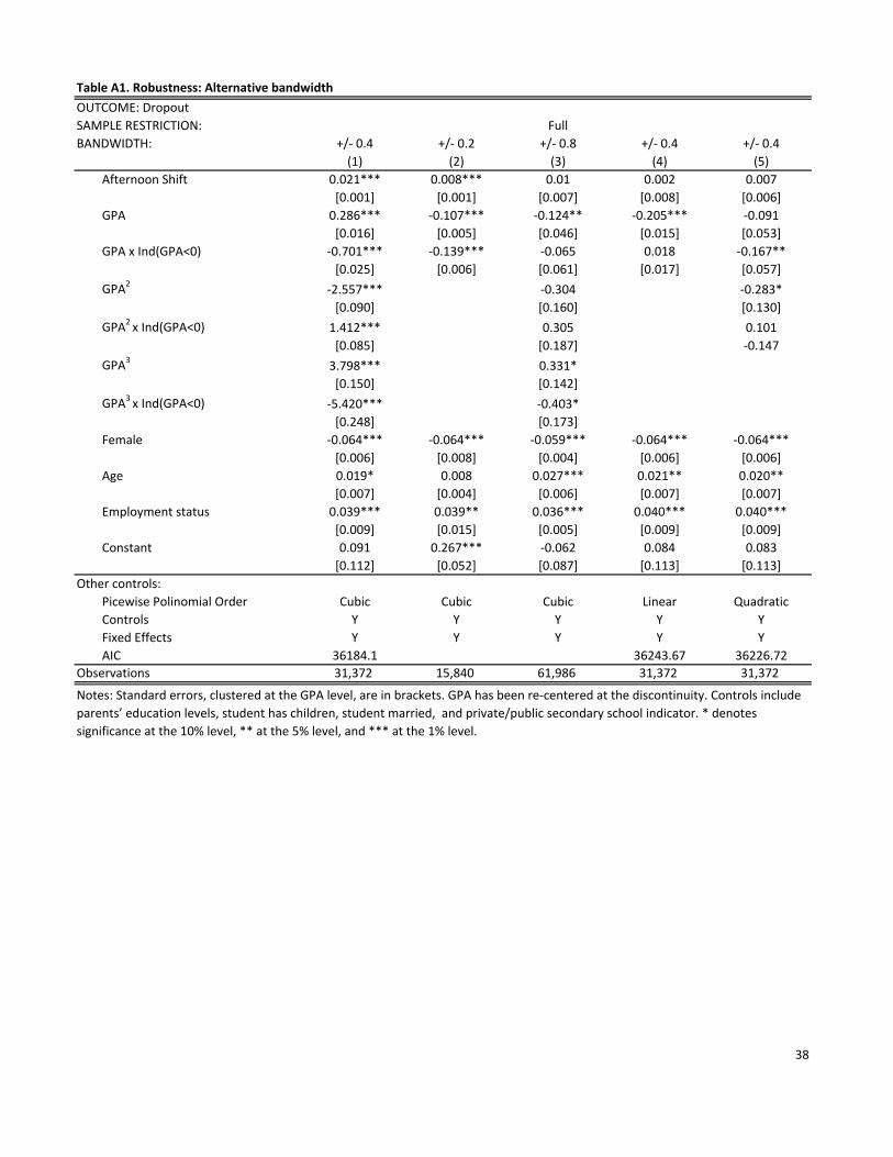
BANDWIDTH: +/‐ 0.4 +/‐ 0.2 +/‐ 0.8 +/‐ 0.4 +/‐ 0.4

(1) (2) (3) (4) (5)

Afternoon Shift 0.021*** 0.008*** 0.01 0.002 0.007

[0.001] [0.001] [0.007] [0.008] [0.006]

GPA 0.286*** ‐0.107*** ‐0.124** ‐0.205*** ‐0.091

[0.016] [0.005] [0.046] [0.015] [0.053]

GPA x Ind(GPA<0) ‐0.701*** ‐0.139*** ‐0.065 0.018 ‐0.167**

[0.025] [0.006] [0.061] [0.017] [0.057]

GPA2‐2.557*** ‐0.304 ‐0.283*

[0.090] [0.160] [0.130]

GPA2 x Ind(GPA<0) 1.412*** 0.305 0.101

[0.085] [0.187] ‐0.147

GPA3

3.798*** 0.331*

[0.150] [0.142]

GPA3 x Ind(GPA<0) ‐5.420*** ‐0.403*

[0.248] [0.173]

Female ‐0.064*** ‐0.064*** ‐0.059*** ‐0.064*** ‐0.064***

[0.006] [0.008] [0.004] [0.006] [0.006]

Age 0.019* 0.008 0.027*** 0.021** 0.020**

[0.007] [0.004] [0.006] [0.007] [0.007]

Employment status 0.039*** 0.039** 0.036*** 0.040*** 0.040***

[0.009] [0.015] [0.005] [0.009] [0.009]

Constant 0.091 0.267*** ‐0.062 0.084 0.083

[0.112] [0.052] [0.087] [0.113] [0.113]

Other controls:

Picewise Polinomial Order Cubic Cubic Cubic Linear Quadratic

Controls Y Y Y Y Y

Fixed Effects Y Y Y Y Y

AIC 36184.1 36243.67 36226.72

Observations 31,372 15,840 61,986 31,372 31,372

38

Table A1. Robustness: Alternative bandwidth

Notes: Standard errors, clustered at the GPA level, are in brackets. GPA has been re‐centered at the discontinuity. Controls include 

parents’ education levels, student has children, student married,  and private/public secondary school indicator. * denotes 

significance at the 10% level, ** at the 5% level, and *** at the 1% level.

Full

39

Figure 1: Structural change analysis

Notes: Estimations based on the methodology used by Card, Mas, y Rothstein (2008).

40

Figure 2: Probability of assignment to the afternoon shift

Notes:  Each circle is the mean of the outcome in an interval of 0.1 around the central point. The solid and dotted 

lines are predicted from local linear regressions with a bandwidth of 0.4.

41

Figure 3: Distribution of students relative to the cutoff

Notes:  Each circle represents the number of students in an interval of 0.1 around the central point. 

The dotted line  is predicted from a local linear regression with a bandwidth of 0.4.

42

Figure 4: Percentage of observations with mising values

Notes:  Each circle is the percent of observations with missing values in an interval of 0.1 around the 

central point.

43

Figure 5: Continuity in observable characteristics

Notes:  Each circle is the mean of the outcome in an interval of 0.1 around the central point. The 

dotted lines are predicted from local linear regressions with a bandwidth of 0.4.

44

Figure 6: Discontinuity in high school GPA

Notes:  Each circle is the mean of the outcome in an interval of 0.1 around the central point. The dotted lines are 

predicted from local linear regressions with a bandwidth of 0.4.

45

Figure 7: Percentage change in high school GPA

Notes:  Each circle is the mean of the outcome in an interval of 0.1 around the central point. The dotted lines are 

predicted from local linear regressions with a bandwidth of 0.4.

46

Figure 8: Discontinuity in the desertion probability

Notes:  Each circle is the mean of the outcome in an interval of 0.1 around the central point. The dotted line is 

predicted from a local linear regression with a bandwidth of 0.4.

47

Figure 9: Discontinuity in the desetion probability by group

Notes:  Each circle is the mean of the outcome in an interval of 0.1 around the central point. The 

dotted lines are predicted from local linear regressions with a bandwidth of 0.4.

48

Figure 10: Drop‐out probability by ranking

Notes:  The bars represent the dropout probability for a student with average characteristics, fixing her position to 

tha last (0=worst) and first place (1=better), for the moorning and afternoon shift respectively, and her re‐

centered middle school GPA fixed in at the threshold (=0) for boh cases.

49

Figure 11: Discontinuity in the probability of admission to UNAM

Notes:  Each circle is the mean of the outcome in an interval of 0.1 around the central point. The 

dotted lines are predicted from local linear regressions with a bandwidth of 0.4.