Embed Size (px)
Citation preview
Double moment microphysics schemes for Numerical Weather
Prediction models: why and how?
F. ChossonM.K. Yau
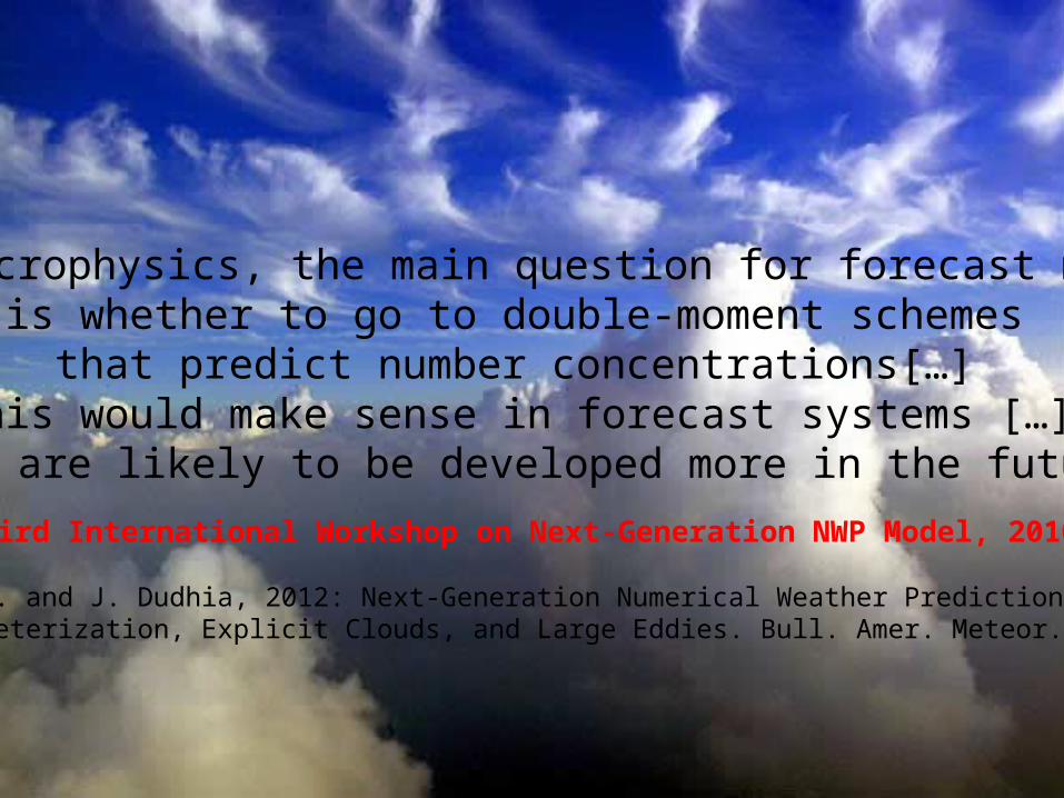
“For microphysics, the main question for forecast models is whether to go to double-moment schemes
that predict number concentrations[…] This would make sense in forecast systems […],
which are likely to be developed more in the future.”
Third International Workshop on Next-Generation NWP Model, 2010.
Hong, S. Y. and J. Dudhia, 2012: Next-Generation Numerical Weather Prediction: BridgingParameterization, Explicit Clouds, and Large Eddies. Bull. Amer. Meteor. Soc.
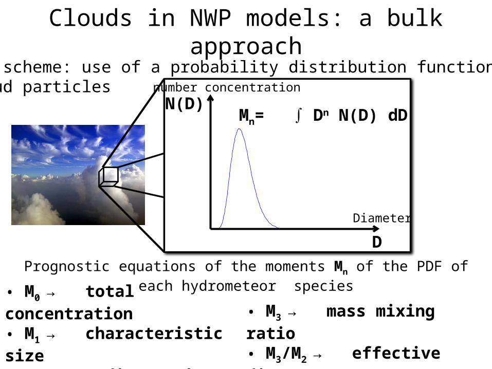
A bulk scheme: use of a probability distribution function (PDF)of cloud particles
N(D)
D
Mn= ∫ Dn N(D) dD
Prognostic equations of the moments Mn of the PDF of each hydrometeor species
number concentration
Diameter
Clouds in NWP models: a bulk approach
• M0 → total concentration• M1 → characteristic size• M2 → sedimentation
fall speed, extinction
• M3 → mass mixing ratio• M3/M2 → effective diameter• M5 → precipitation flux• M6 → radar reflectivity
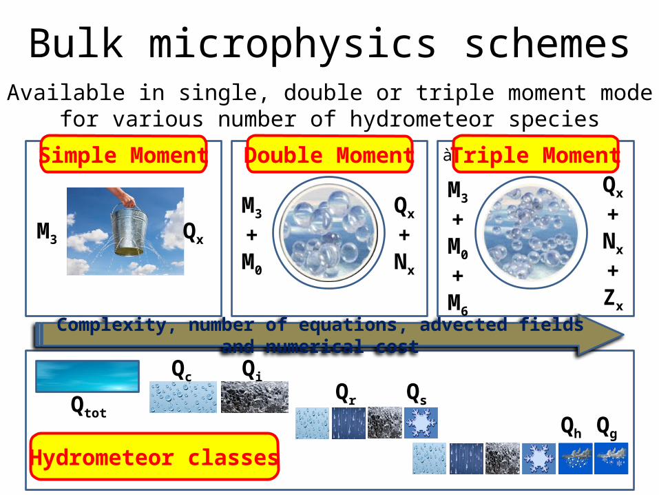
Available in single, double or triple moment mode for various number of hydrometeor species
à Simple Moment à Double Moment à Triple Moment
Qx Qx +Nx
Qx
+Nx
+Zx
Simple Moment Double Moment Triple Moment
M3
M3
+M0
M3
+M0
+M6
Bulk microphysics schemes
Qtot
Qc QiQsQr
QgQh
Hydrometeor classes
Complexity, number of equations, advected fields and numerical cost
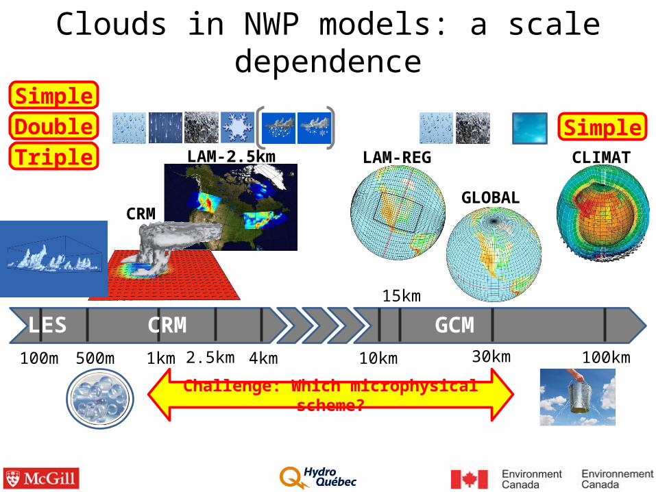
LAM-2.5km LAM-REG
GLOBAL
GCM100m 500m 1km 4km 10km 30km 100km2.5km
15km
CRMLES
Challenge: Which microphysical scheme?
SimpleDoubleTriple
Simple
CRM
CLIMAT
Clouds in NWP models: a scale dependence
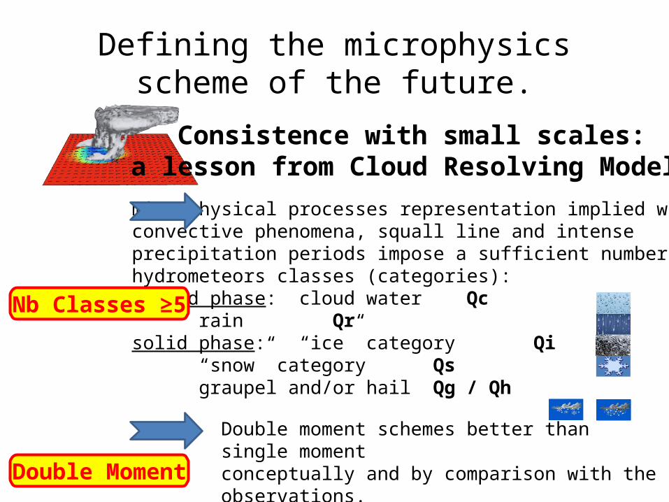
Defining the microphysics scheme of the future.
Consistence with small scales:a lesson from Cloud Resolving Models
microphysical processes representation implied withinconvective phenomena, squall line and intenseprecipitation periods impose a sufficient number ofhydrometeors classes (categories):liquid phase: cloud water Qc
rain Qrsolid phase: “ice” category Qi
“snow” category Qsgraupel and/or hail Qg / Qh
Nb Classes ≥5
Double Moment
Double moment schemes better than single momentconceptually and by comparison with the observations.(e.g. Lim and Hong, 2009; Morrison et al., 2009; Milbrandt et al., 2009?)
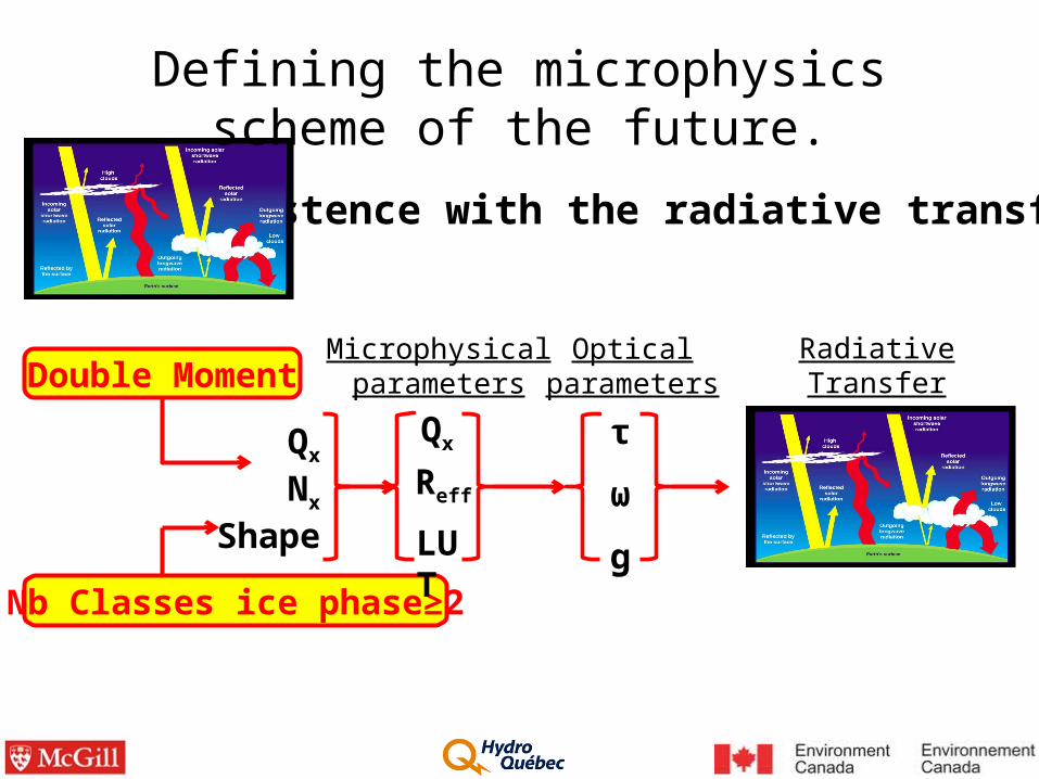
Consistence with the radiative transfer:
Qx
Reff
τ
ω
g
Microphysicalparameters
Opticalparameters
RadiativeTransfer
Qx
Nx
Shape
Double Moment
Nb Classes ice phase≥2
Defining the microphysics scheme of the future.
LUT
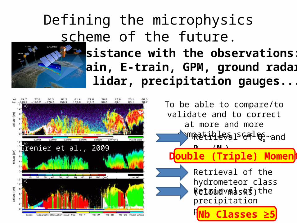
Consistance with the observations:A-train, E-train, GPM, ground radar
and lidar, precipitation gauges...
Grenier et al., 2009Retrieval of Qx and Reff (Nx)
To be able to compare/to validate and to correct at more and more
compatibles scales…
Retrieval of the hydrometeor class (cloud masks)Retrieval of the precipitation profiles
Double (Triple) Moment
Nb Classes ≥5
Defining the microphysics scheme of the future.
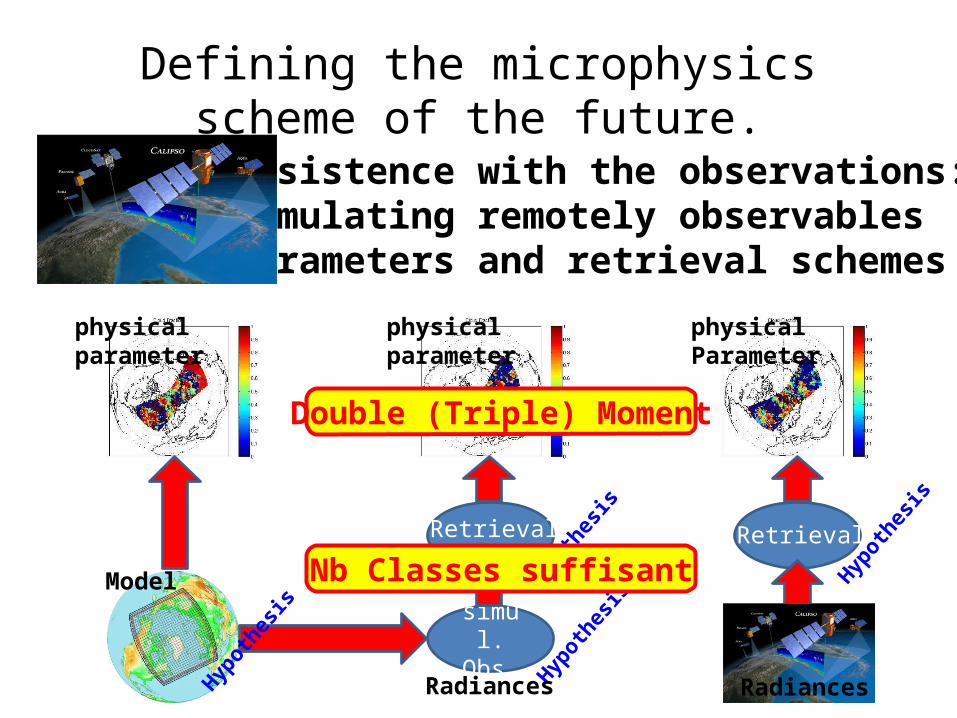
Consistence with the observations:simulating remotely observables parameters and retrieval schemes
simul. Obs.
Retrieval
physicalparameter
physicalparameter
physicalParameter
Model
Hyp
othe
sisH
ypot
hesi
s
Hyp
othe
sis
Hyp
othe
sis
Radiances Radiances
Double (Triple) Moment
Nb Classes suffisant
Defining the microphysics scheme of the future.
Retrieval
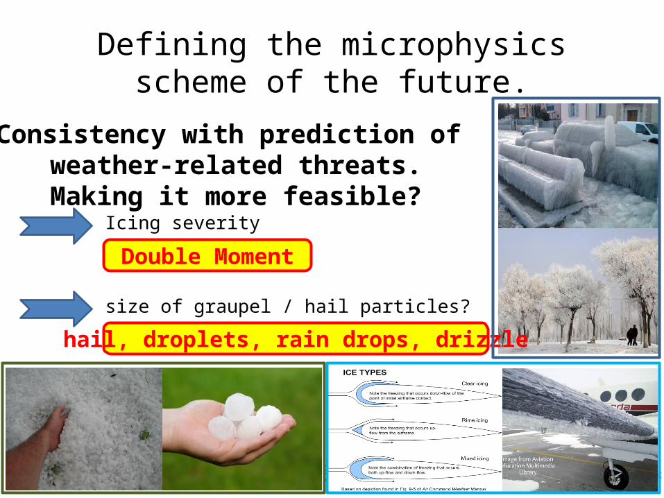
Consistency with prediction of weather-related threats.Making it more feasible?Icing severity
size of graupel / hail particles?
Double Moment
Defining the microphysics scheme of the future.
hail, droplets, rain drops, drizzle
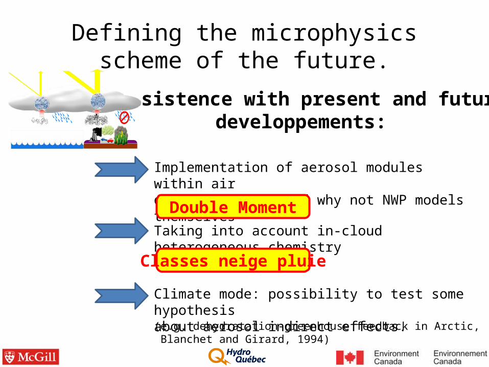
Consistence with present and futurdeveloppements:
Implementation of aerosol modules within air quality models, and why not NWP models themselves
Taking into account in-cloud heterogeneous chemistry
Climate mode: possibility to test some hypothesisabout aerosol indirect effects.(e.g. dehydratation-greenhouse feedback in Arctic, Blanchet and Girard, 1994)
Double Moment
Classes neige pluie
Defining the microphysics scheme of the future.
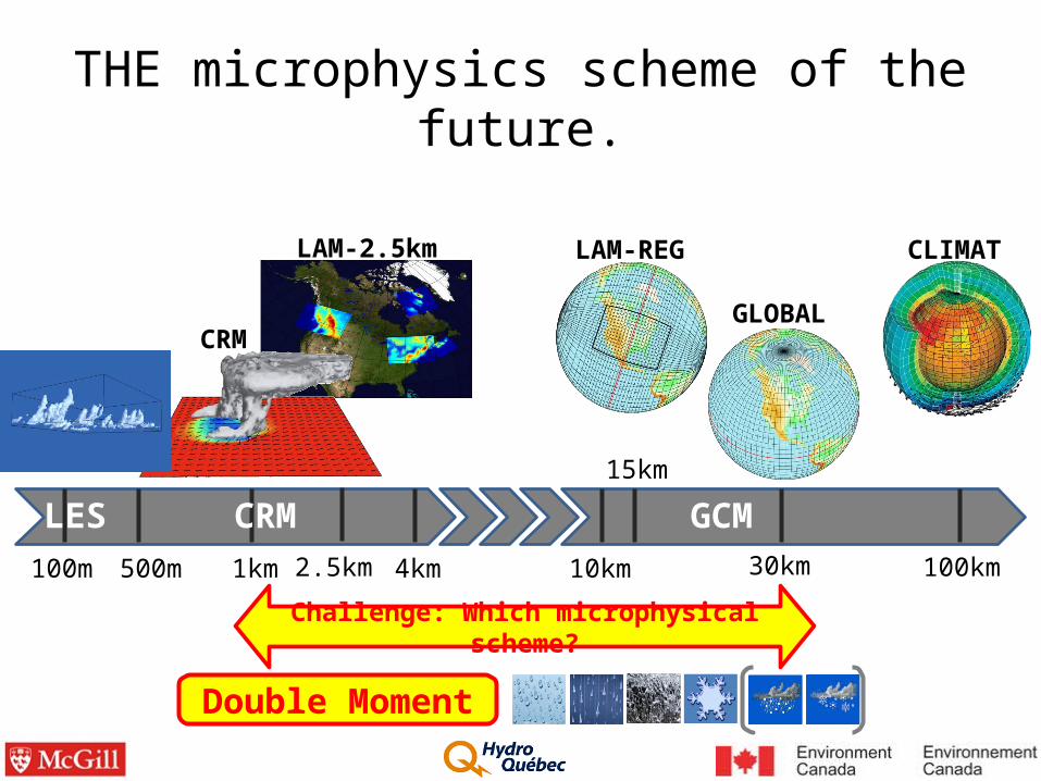
GCM
CRM
LAM-2.5km LAM-REG
GLOBAL
CLIMAT
100m 500m 1km 4km 10km 30km 100km2.5km
15km
Double Moment
Challenge: Which microphysical scheme?
LES CRM
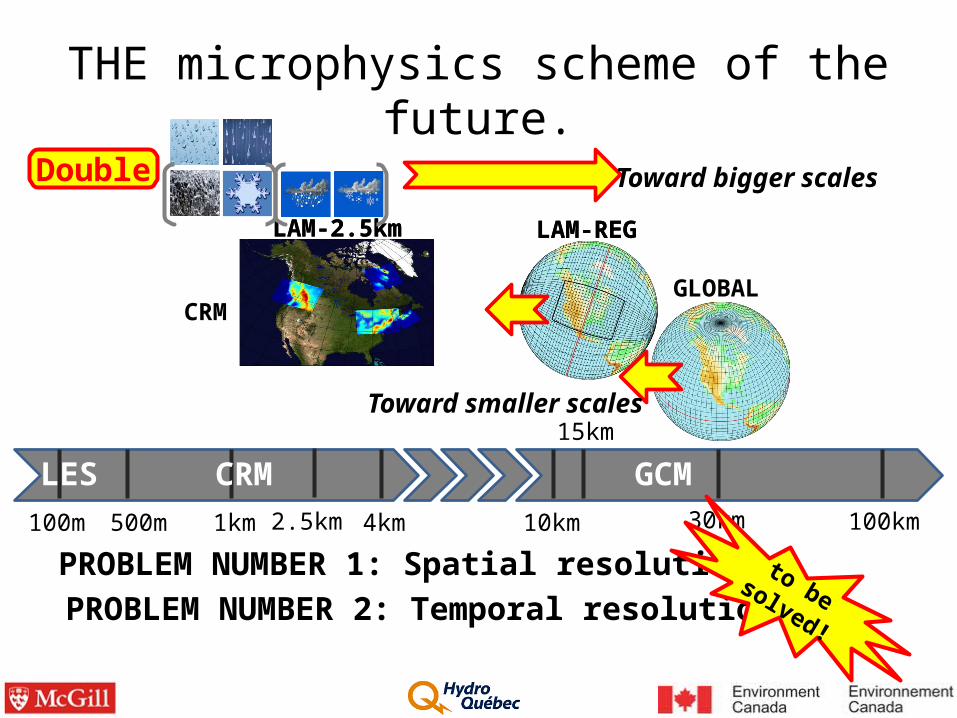
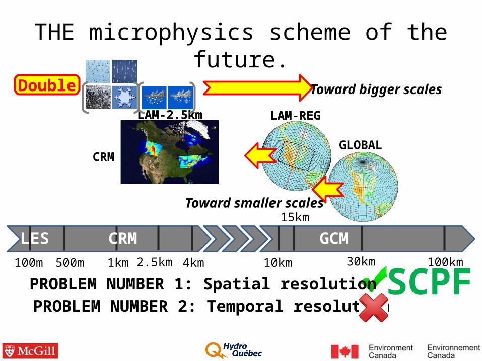
THE microphysics scheme of the future.
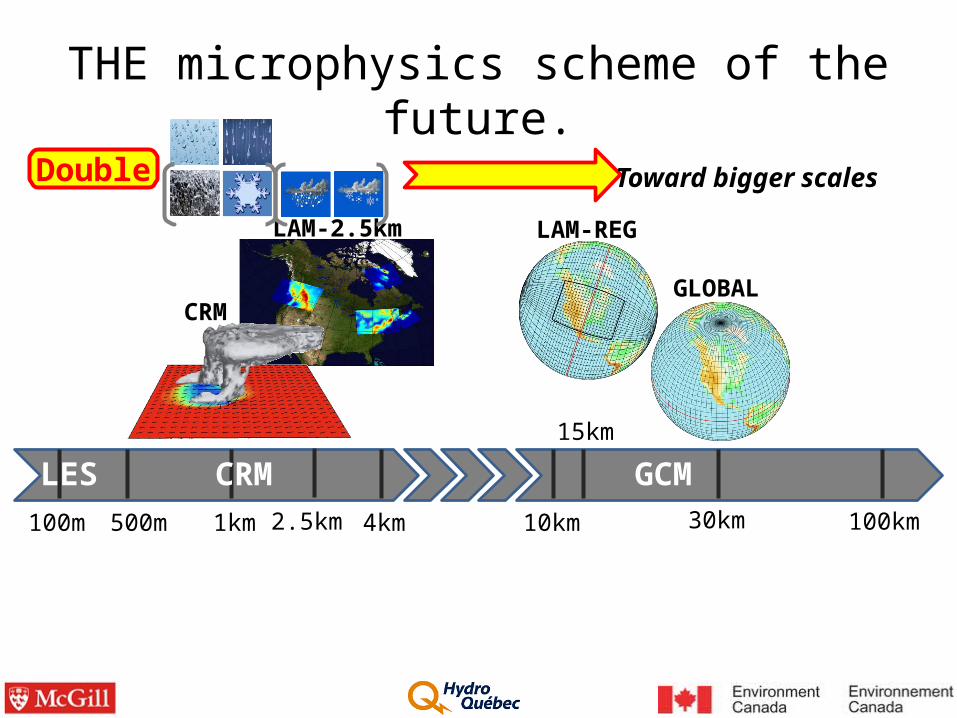
LAM-2.5km LAM-REG
GLOBAL
GCM100m 500m 1km 4km 10km 30km 100km2.5km
15km
CRMLES
Double
CRM
Toward bigger scales
THE microphysics scheme of the future.
GLOBAL
GCM100m 500m 1km 4km 10km 30km 100km2.5km
15km
CRMLES
CRM
LAM-2.5km LAM-REG
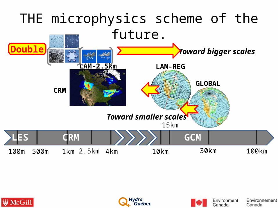
Double Toward bigger scales
Toward smaller scales
THE microphysics scheme of the future.
LAM-2.5km LAM-REG
GLOBAL
GCM100m 500m 1km 4km 10km 30km 100km2.5km
15km
CRMLES
CRM
PROBLEM NUMBER 1: Spatial resolutionPROBLEM NUMBER 2: Temporal resolution
to be solved!
LAM-2.5km LAM-REG
Double Toward bigger scales
Toward smaller scales
THE microphysics scheme of the future.

tqdqPDFa
s
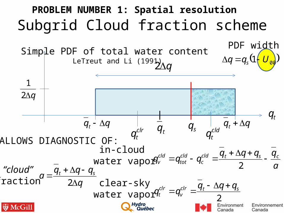
PROBLEM NUMBER 1: Spatial resolution
motto:
keep it simple!
Subgrid Cloud fraction schemeTompkins,
2005
tq
Simple PDF of total water content LeTreut and Li (1991)
q21
tq qq t
q2
qq t sq
cldtqclr
tq
q
qqqa st
2
a
qqqqqqq cstcld
ccldtot
cldv
2
2stclr
vclrt
qqqqq
“cloud”fraction
in-cloud water vapor
clear-skywater vapor
001 Uqq s PDF width
ALLOWS DIAGNOSTIC OF:
PROBLEM NUMBER 1: Spatial resolution
Subgrid Cloud fraction scheme
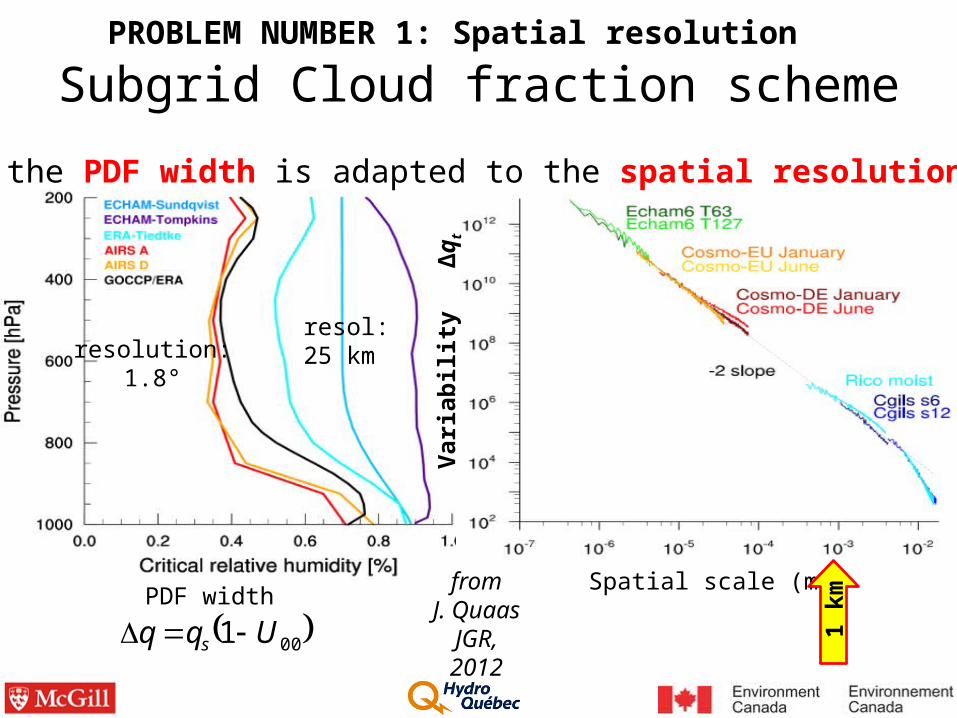
fromJ. Quaas
JGR,2012
001 Uqq s PDF width
Varia
bilit
y ∆
q t
the PDF width is adapted to the spatial resolution!
Spatial scale (m)
1 km
resolution:1.8°
resol:25 km
PROBLEM NUMBER 1: Spatial resolution
Subgrid Cloud fraction scheme
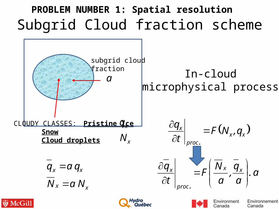
a
subgrid cloudfraction In-cloud
microphysical process
xxproc
x q,NFt
q
.
a.a
q,
a
NF
t
q xx
proc
x
.
CLOUDY CLASSES: Pristine IceSnowCloud droplets x
x
N
q
xx
xx
NaN
qaq
PROBLEM NUMBER 1: Spatial resolution
Subgrid Cloud fraction scheme
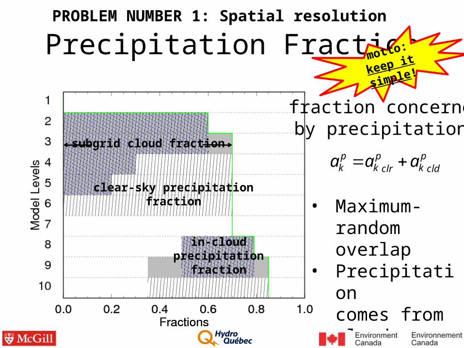
Precipitation Fraction
fraction concernedby precipitation?
cldpkclr
pk
pk aaa
• Maximum-random overlap
• Precipitationcomes from clouds above
subgrid cloud fraction
clear-sky precipitationfraction
in-cloudprecipitation
fraction
PROBLEM NUMBER 1: Spatial resolution
motto:
keep it simple!
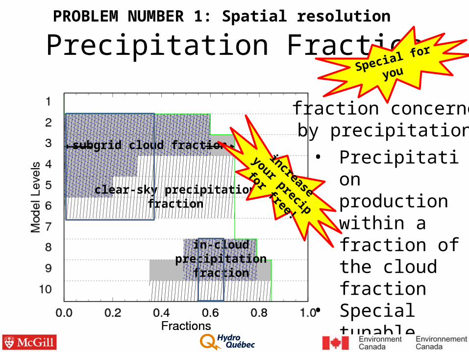
Precipitation Fraction
fraction concernedby precipitation?
• Precipitation production within a fraction of the cloud fraction
• Special tunable parameter!
subgrid cloud fraction
clear-sky precipitationfraction
in-cloudprecipitation
fraction
PROBLEM NUMBER 1: Spatial resolution
Special for you
increase your
precip for free!
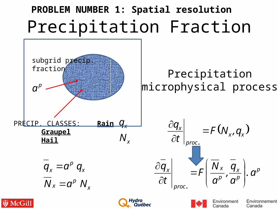
Precipitationmicrophysical process
xxproc
x q,NFt
q
.
ppx
p
x
proc
x a.a
q,
a
NF
t
q
.
PRECIP. CLASSES: RainGraupelHail x
x
N
q
xp
x
xp
x
NaN
qaq
pa
subgrid precip.fraction
Precipitation FractionPROBLEM NUMBER 1: Spatial resolution
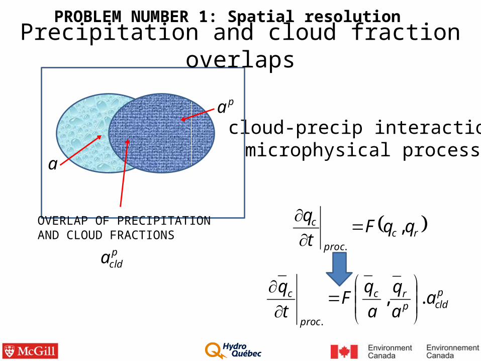
pacloud-precip interactionmicrophysical process
rcproc
c qqFt
q,
.
pcldp
rc
proc
c aa
q
a
qF
t
q.,
.
OVERLAP OF PRECIPITATIONAND CLOUD FRACTIONS
pclda
a
Precipitation and cloud fraction overlapsPROBLEM NUMBER 1: Spatial resolution
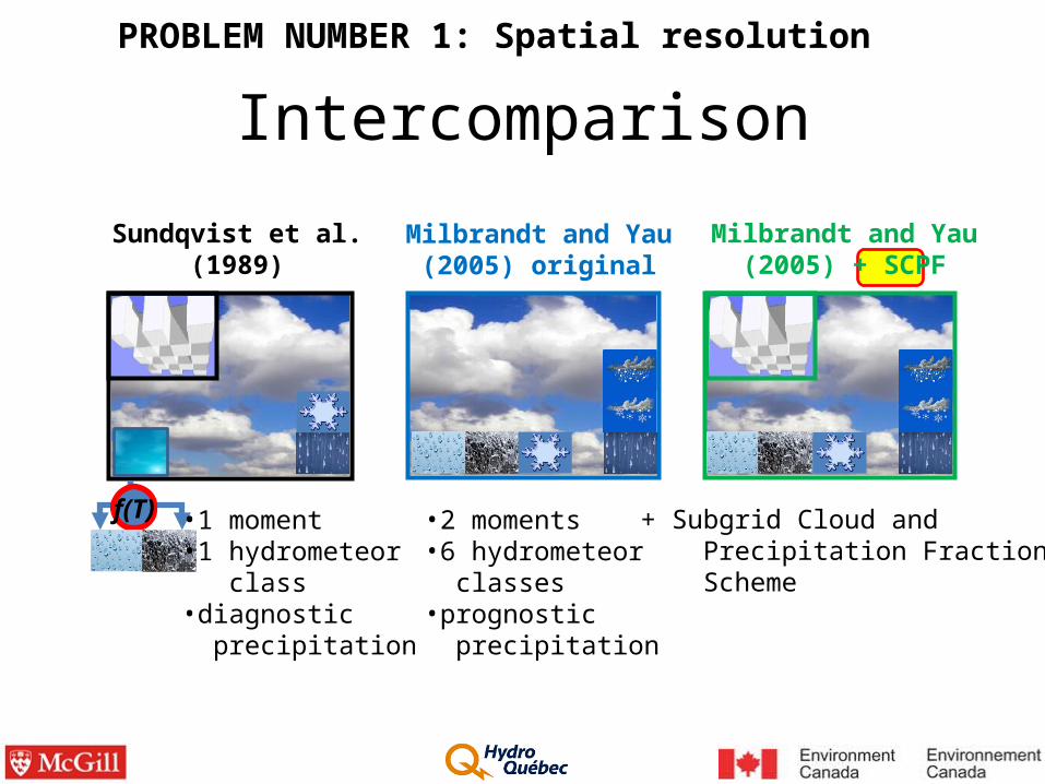
Intercomparison
f(T)
Milbrandt and Yau(2005) original
Milbrandt and Yau(2005) + SCPF
Sundqvist et al.(1989)
•1 moment•1 hydrometeor class•diagnostic precipitation
•2 moments•6 hydrometeor classes•prognostic precipitation
+ Subgrid Cloud and Precipitation Fraction Scheme
PROBLEM NUMBER 1: Spatial resolution
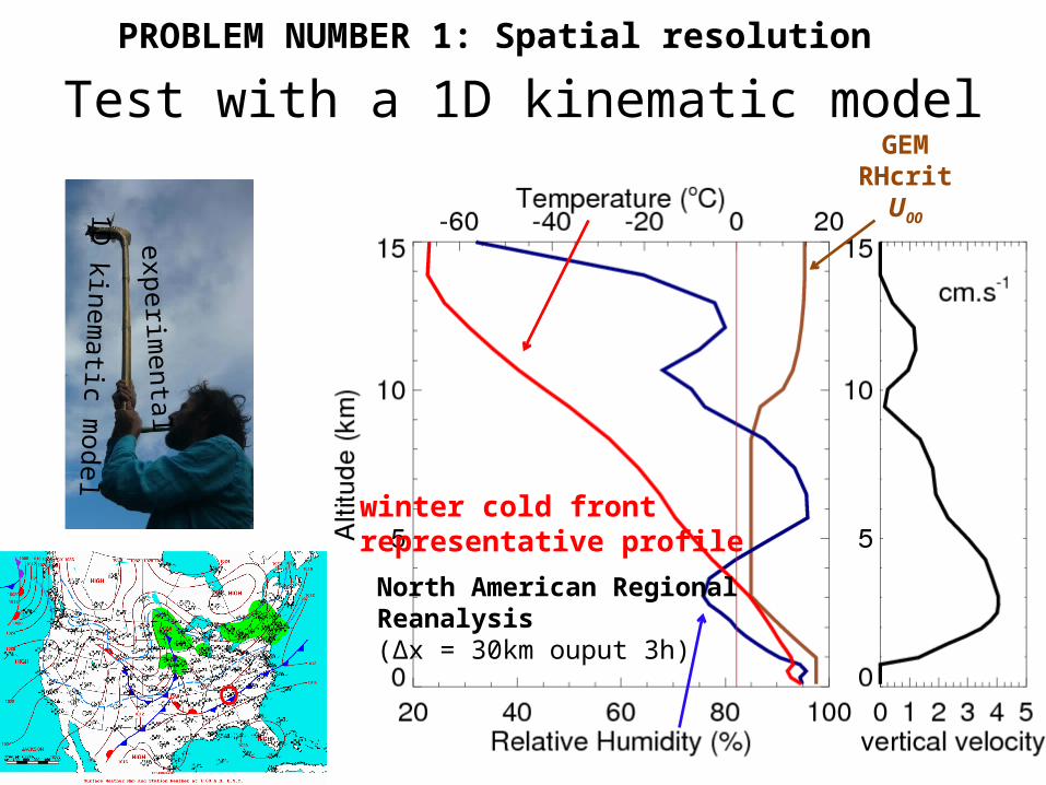
North American RegionalReanalysis(∆x = 30km ouput 3h)
GEMRHcrit
U00
winter cold front representative profile
Test with a 1D kinematic model
experimental
1D kinem
atic model
PROBLEM NUMBER 1: Spatial resolution

1D kinematic intercomparisonMilbrandt & Yau original M&Y with SCPF Sundqvist
+ +
PROBLEM NUMBER 1: Spatial resolution
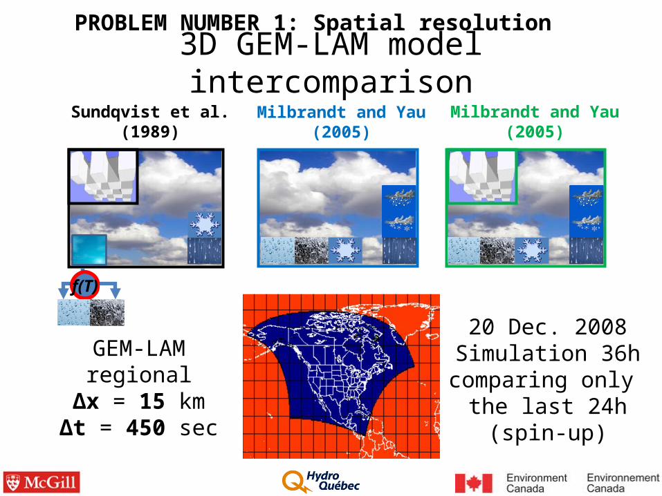
Milbrandt and Yau(2005)
3D GEM-LAM model intercomparison
f(T)
Milbrandt and Yau(2005)
Sundqvist et al.(1989)
GEM-LAMregional
∆x = 15 km∆t = 450 sec
20 Dec. 2008Simulation 36hcomparing only
the last 24h(spin-up)
PROBLEM NUMBER 1: Spatial resolution
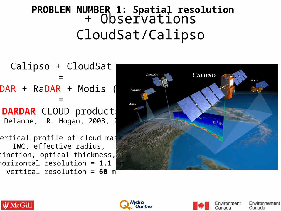
+ Observations CloudSat/Calipso
Calipso + CloudSat=
LiDAR + RaDAR + Modis (IR)=
DARDAR CLOUD products(J. Delanoe, R. Hogan, 2008, 2010)
vertical profile of cloud mask,IWC, effective radius,
extinction, optical thickness, ...horizontal resolution = 1.1 km
vertical resolution = 60 m
PROBLEM NUMBER 1: Spatial resolution
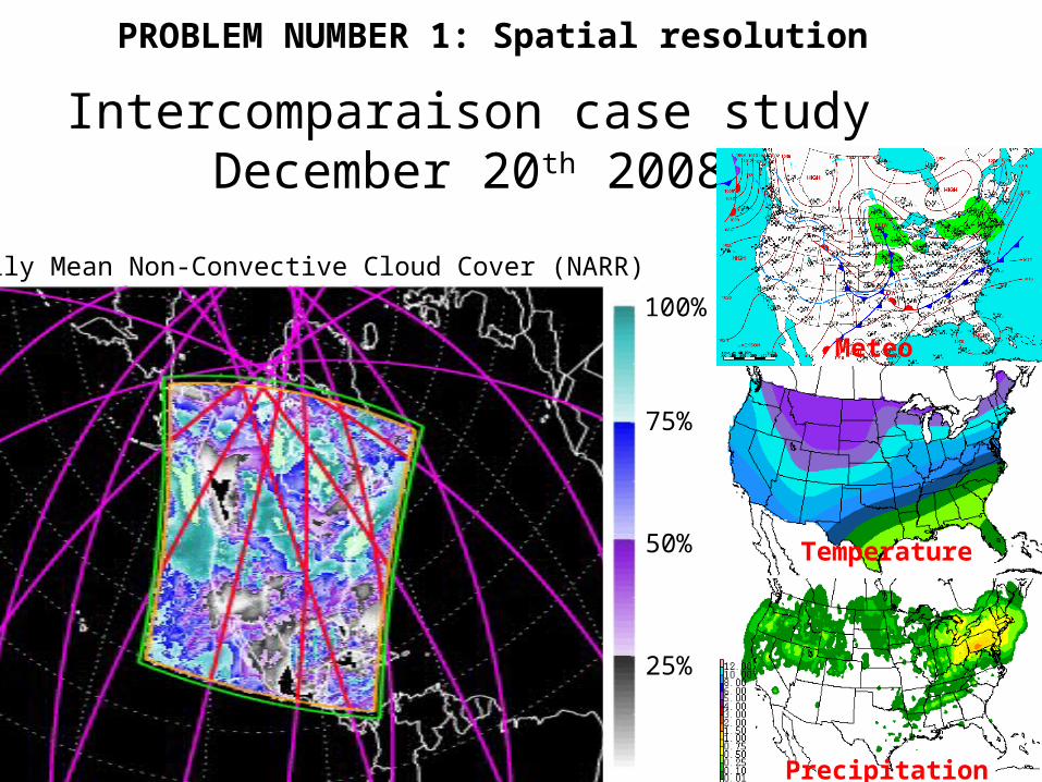
Intercomparaison case study December 20th 2008
Daily Mean Non-Convective Cloud Cover (NARR)
25%
50%
75%
100%
Precipitation
Temperature
Meteo
PROBLEM NUMBER 1: Spatial resolution
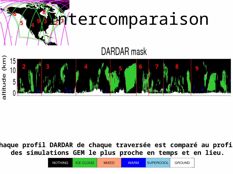
Intercomparaison
2
2345
67
8
9
3 4 5 6 7 8 9
Chaque profil DARDAR de chaque traversée est comparé au profil des simulations GEM le plus proche en temps et en lieu.
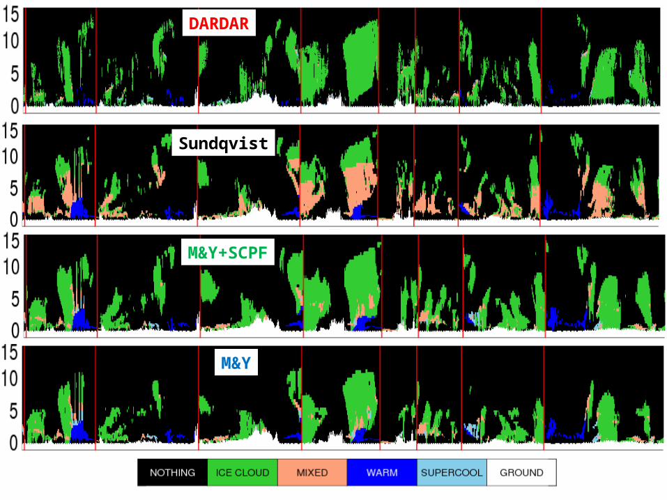
2 3 4 5 6 7 8 9
DARDAR
Sundqvist
M&Y+SCPF
M&Y
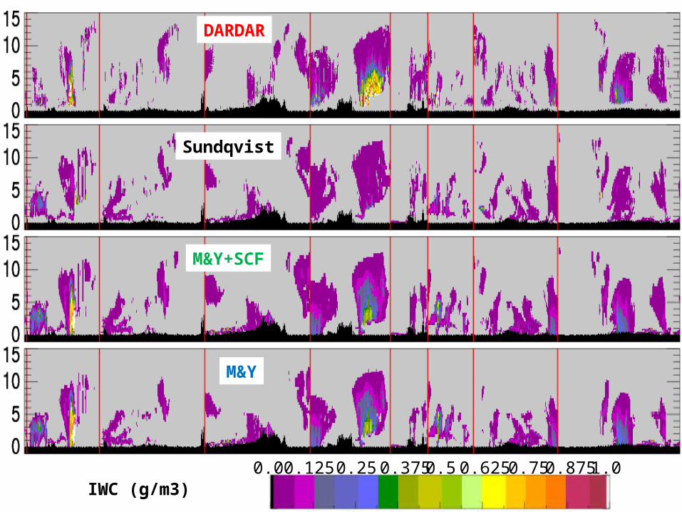
DARDAR
Sundqvist
M&Y+SCF
M&Y
0.0 0.125IWC (g/m3)
0.25 0.375 0.5 0.625 0.75 0.875 1.0
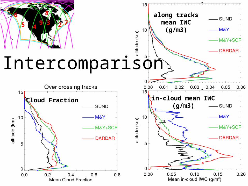
Intercomparison
2345
67
8
9
Cloud Fraction
along tracksmean IWC
(g/m3)
in-cloud mean IWC(g/m3)
LAM-2.5km LAM-REG
GLOBAL
GCM100m 500m 1km 4km 10km 30km 100km2.5km
15km
CRMLES
CRM
PROBLEM NUMBER 1: Spatial resolutionPROBLEM NUMBER 2: Temporal resolution
LAM-2.5km LAM-REG
Double Toward bigger scales
Toward smaller scales
THE microphysics scheme of the future.
SCPF
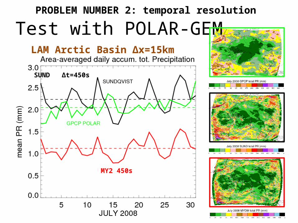
SUND ∆t=450s
LAM Arctic Basin ∆x=15km
Test with POLAR-GEMPROBLEM NUMBER 2: temporal resolution
MY2 450s
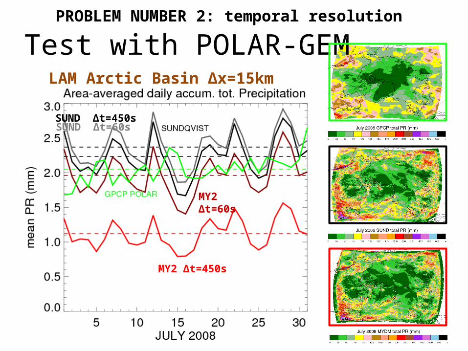
SUND ∆t=450sSUND ∆t=60s
MY2 ∆t=450s
LAM Arctic Basin ∆x=15km
Test with POLAR-GEMPROBLEM NUMBER 2: temporal resolution
MY2 ∆t=60s
PROBLEM NUMBER 2: temporal resolution
Microphysical sub-time step
sedmicradv t
q
t
q
t
q
t
q
t
F
ρ
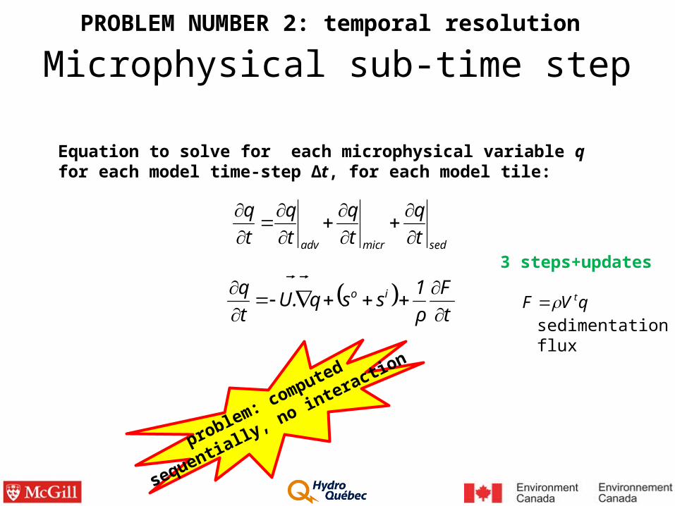
1ssq.U
t
q io
Equation to solve for each microphysical variable qfor each model time-step ∆t, for each model tile:
problem: computed
sequentially, no interaction
3 steps+updates
qVF tsedimentationflux
Microphysical sub-time step
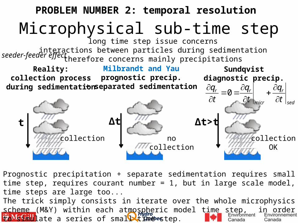
∆t>t
Sundqvistdiagnostic precip.
Milbrandt and Yauprognostic precip.
+ separated sedimentation
long time step issue concernsinteractions between particles during sedimentation
therefore concerns mainly precipitations
collectionOK
nocollection
collection
t ∆t
Reality:collection process
during sedimentation
Prognostic precipitation + separate sedimentation requires small time step, requires courant number = 1, but in large scale model, time steps are large too...The trick simply consists in iterate over the whole microphysics scheme (M&Y) within each atmospheric model time step, in order to simulate a series of small time step.
PROBLEM NUMBER 2: temporal resolution
seeder-feeder effect
sed
r
micr
rr
t
q
t
q
t
q
0
sedmicradv t
q
t
q
t
q
t
q
n
i sedimicriadvi t
q
t
q
t
q
t
q
1
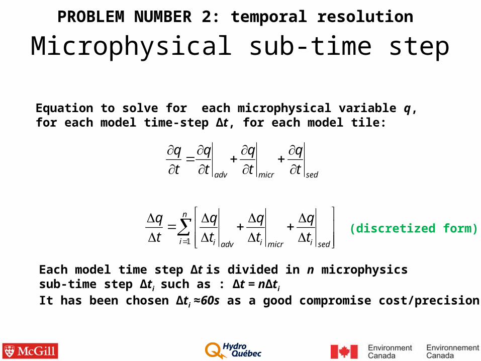
Each model time step ∆t is divided in n microphysicssub-time step ∆ti such as : ∆t = n∆ti It has been chosen ∆ti ≈60s as a good compromise cost/precision.
Equation to solve for each microphysical variable q, for each model time-step ∆t, for each model tile:
(discretized form)
PROBLEM NUMBER 2: temporal resolution
Microphysical sub-time step

LAM Arctic Basin ∆x=15km
Test with POLAR-GEMPROBLEM NUMBER 2: temporal resolution
SUND 450sSUND 60s
MY2 450s
MY2 60sMY2 450s sub-time step at 60s

The problem that resists
Numerical cost!
∆t = 450 sec
reference
x 1.2Other avenues?
x 2.3 !
∆t = 450 sec
dtmicro=60 sec
∆x = 15km Sundqvist
Milbrandt& Yau
PROBLEM NUMBER 2: temporal resolution
∆x= 15km
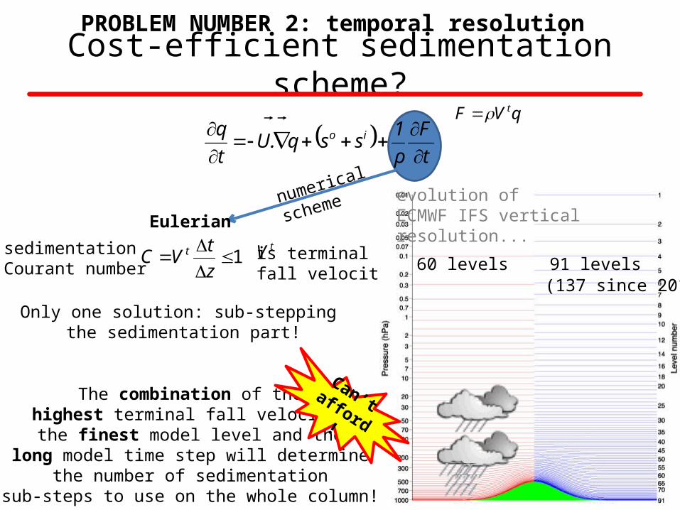
Can’t afford !
Cost-efficient sedimentation scheme?PROBLEM NUMBER 2: temporal resolution
t
F
ρ
1ssq.U
t
q io
Eulerian
qVF t
1
z
tVC t tV is terminal
fall velocitysedimentationCourant number
numerical
scheme evolution ofECMWF IFS verticalresolution...
60 levels 91 levels(137 since 2013)
The combination of thehighest terminal fall velocity,
the finest model level and thelong model time step will determine
the number of sedimentationsub-steps to use on the whole column!
Can’t afford !
Only one solution: sub-stepping the sedimentation part!
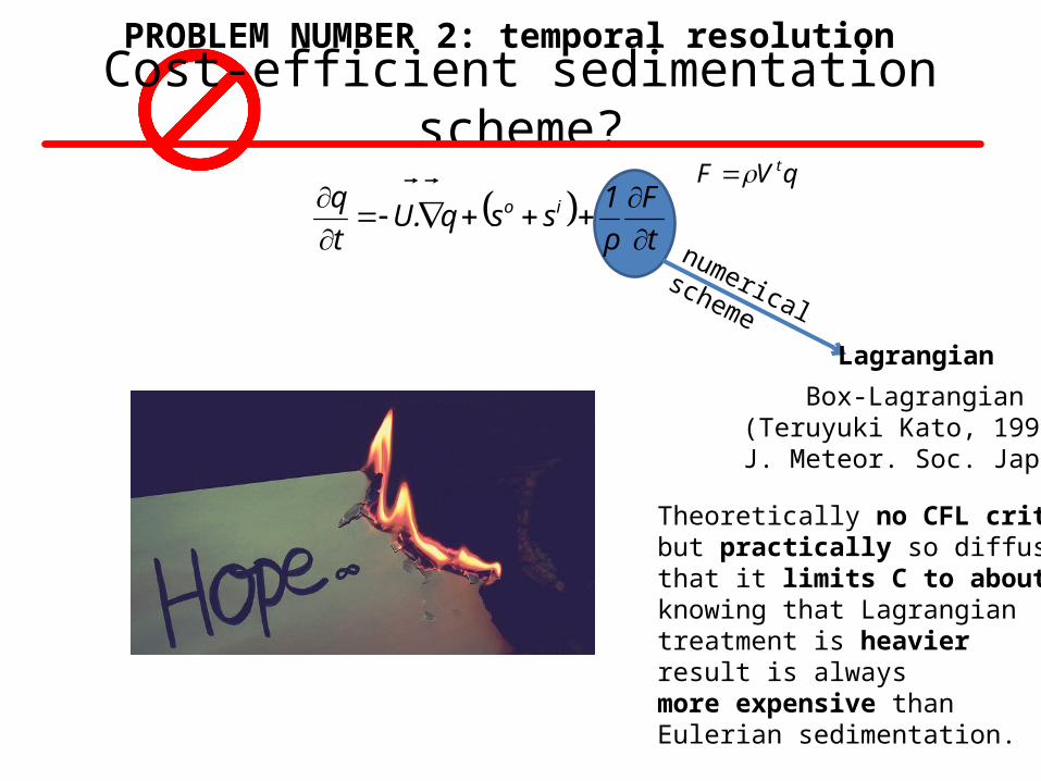
Cost-efficient sedimentation scheme?PROBLEM NUMBER 2: temporal resolution
t
F
ρ
1ssq.U
t
q io
Lagrangian
Box-Lagrangian(Teruyuki Kato, 1995, J. Meteor. Soc. Japan)
qVF t
Theoretically no CFL criteriabut practically so diffusivethat it limits C to about 2-3knowing that Lagrangian treatment is heavierresult is alwaysmore expensive than Eulerian sedimentation.
numericalscheme

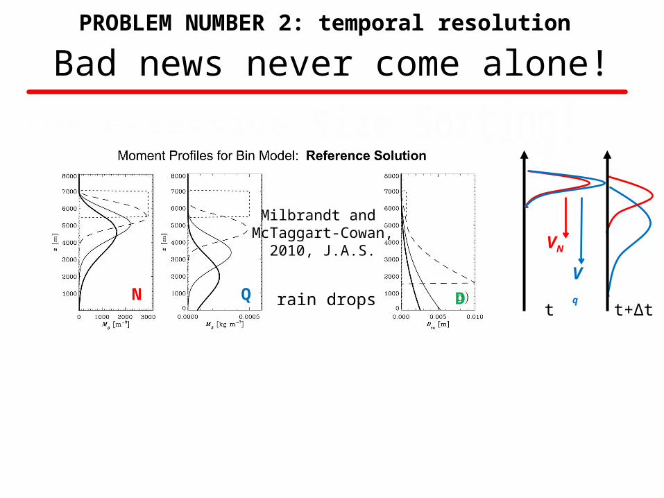
Bad news never come alone!
Mass qx and concentration Nx have different fall velocities Vq > VN
(they are proportional and the proportion p depends on the assumed shape of the size distribution).
t t+∆t
PROBLEM NUMBER 2: temporal resolution
Vq
VN
The goal is to mimic size sorting: bigger particles falls faster
Bad news never come alone!
t t+∆t
PROBLEM NUMBER 2: temporal resolution
Vq
VN
N Q D
Milbrandt and McTaggart-Cowan,
2010, J.A.S.
rain drops
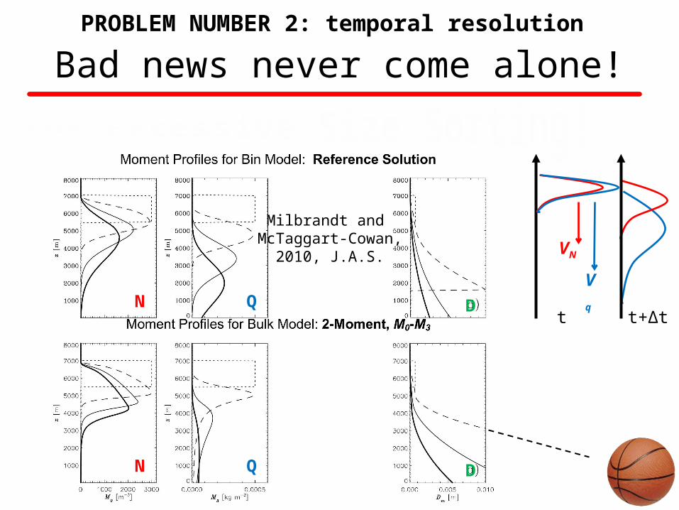
Bad news never come alone!
t t+∆t
PROBLEM NUMBER 2: temporal resolution
Vq
VN
N Q D
N Q D
Milbrandt and McTaggart-Cowan,
2010, J.A.S.

PROBLEM NUMBER 2: temporal resolution
Solutions:rain drop spontaneous break-up?
yes, but... how about ice particles?Limiting mean mass diameter?
yes, but... that implies inventing new particles
Bad news never come alone!
PROBLEM NUMBER 2: temporal resolution
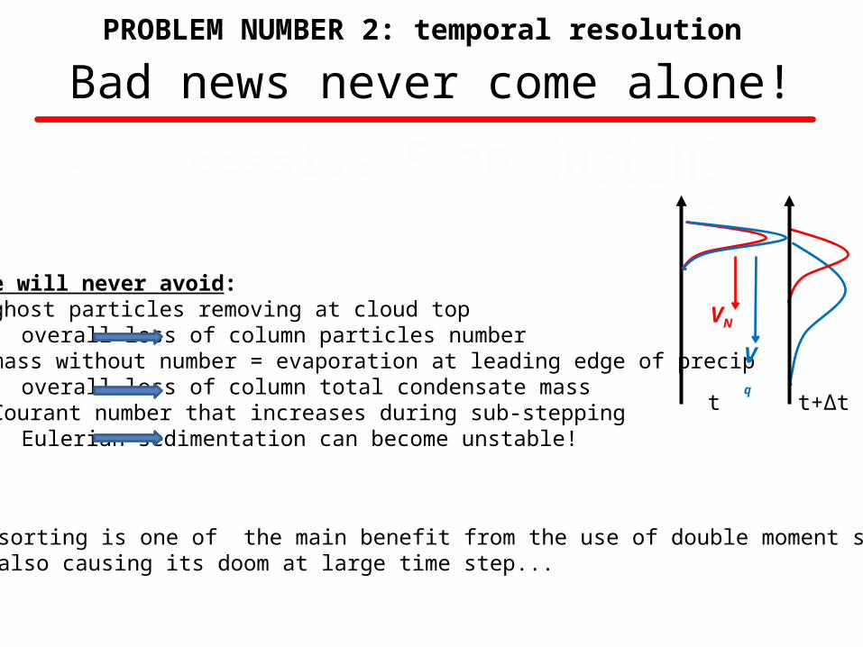
We will never avoid:•ghost particles removing at cloud top
overall loss of column particles number•mass without number = evaporation at leading edge of precip
overall loss of column total condensate mass•Courant number that increases during sub-stepping
Eulerian sedimentation can become unstable!
t t+∆t
Vq
VN
Size sorting is one of the main benefit from the use of double moment schemesit’s also causing its doom at large time step...
Bad news never come alone!
c
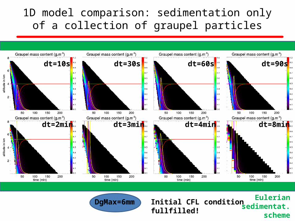
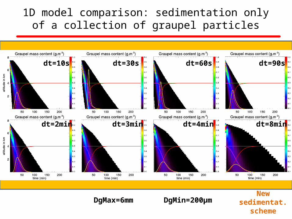
1D model comparison: sedimentation only of a collection of graupel particles
Euleriansedimentat.
scheme
dt=10s dt=30s dt=60s dt=90s
dt=2min dt=3min dt=4min dt=8min
DgMax=6mm Initial CFL conditionfullfilled!
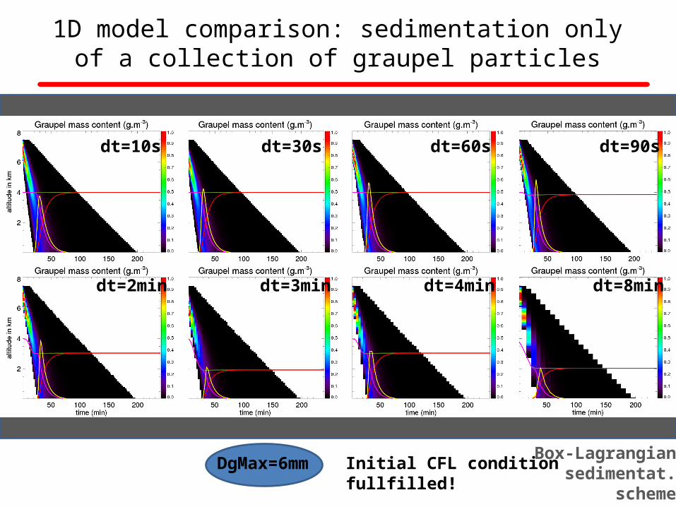
c
1D model comparison: sedimentation only of a collection of graupel particles
Box-Lagrangiansedimentat.
scheme
dt=10s dt=30s dt=60s dt=90s
dt=2min dt=3min dt=4min dt=8min
DgMax=6mm Initial CFL conditionfullfilled!
Cost-efficient sedimentation scheme!PROBLEM NUMBER 2: temporal resolution
We have a Solution for You!
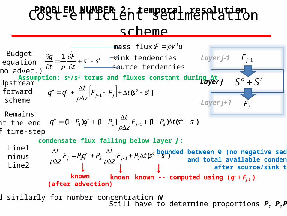
Cost-efficient sedimentation scheme
io ssz
F
t
q
1
mass flux: qVF t
source tendenciessink tendenciesBudget
equation(no advec.)
Upstreamforwardscheme
)( iojj sstFF
z
tqq
1
Assumption: so/si terms and fluxes constant during ∆t Layer j
Layer j-1 1jF
jF
io SS
Remainsat the end
of time-step)()()()( io
j sstPFz
tPqPq
3121 111
Layer j+1
Line1minusLine2
)( iojj sstPF
z
tPqPF
z
t
3121
condensate flux falling below layer j :
bounded between 0 (no negative sedim.)and total available condensate
after source/sink termsknown
(after advection)known known -- computed using (q- + Fj-1 )
... And similarly for number concentration NStill have to determine proportions P1 P2 P3 ...
PROBLEM NUMBER 2: temporal resolution
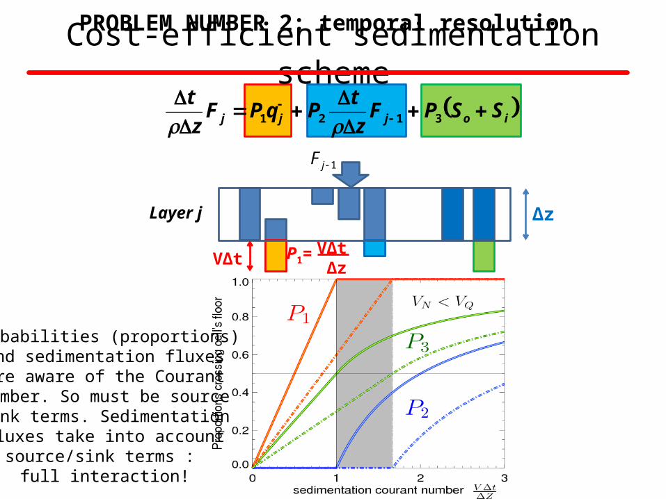
iojjj SSPFz
tPqPF
z
t
3121
V∆tV∆t ∆z
Layer j
1jF
∆z
P1=
Cost-efficient sedimentation schemePROBLEM NUMBER 2: temporal resolution
Probabilities (proportions)and sedimentation fluxesare aware of the Courant
number. So must be sourcesink terms. Sedimentation
fluxes take into accountsource/sink terms :
full interaction!

Cost-efficient sedimentation scheme
Lets fix a maximum mean mass diameter so that D ≤ Dmax (from obs., tunable). It follows that there is a maximum terminal fall velocity It follows that both moment outgoing sedimentation fluxes are related and bounded:
t t+∆t
dqN Dc
pFF
max
Avoiding excessive size sorting
PROBLEM NUMBER 2: temporal resolution
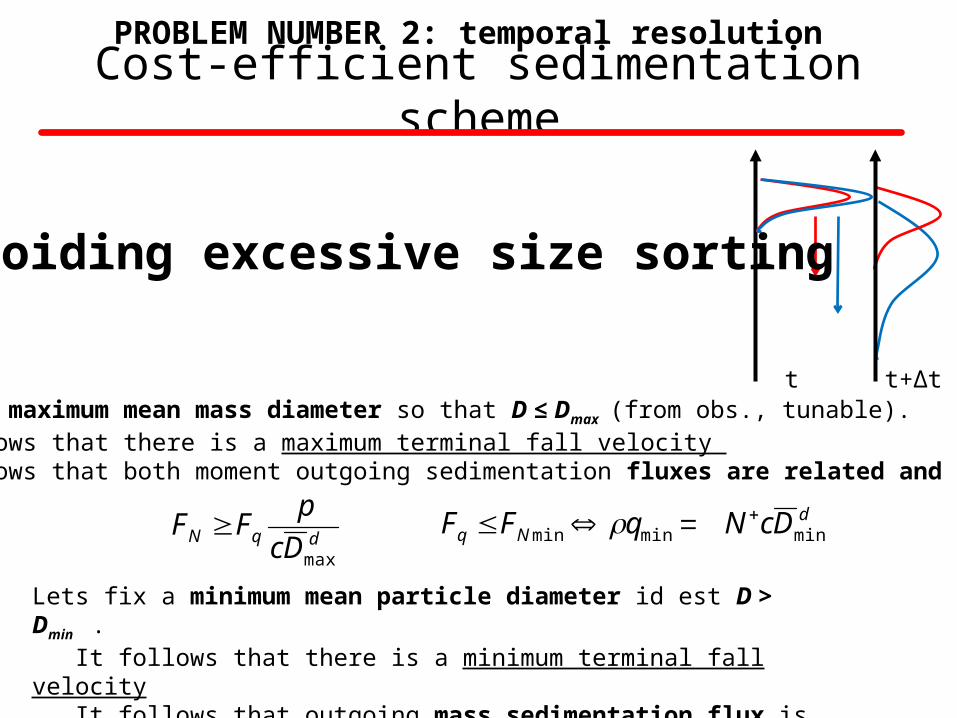
Cost-efficient sedimentation scheme
t t+∆t
dqN Dc
pFF
max
dNq DcNqFF minminmin
Lets fix a minimum mean particle diameter id est D > Dmin . It follows that there is a minimum terminal fall velocity It follows that outgoing mass sedimentation flux is bounded so that the remaining particles (if any, constrained by FN) are always bigger than this minimum.
Lets fix a maximum mean mass diameter so that D ≤ Dmax (from obs., tunable). It follows that there is a maximum terminal fall velocity It follows that both moment outgoing sedimentation fluxes are related and bounded:
Avoiding excessive size sorting
PROBLEM NUMBER 2: temporal resolution
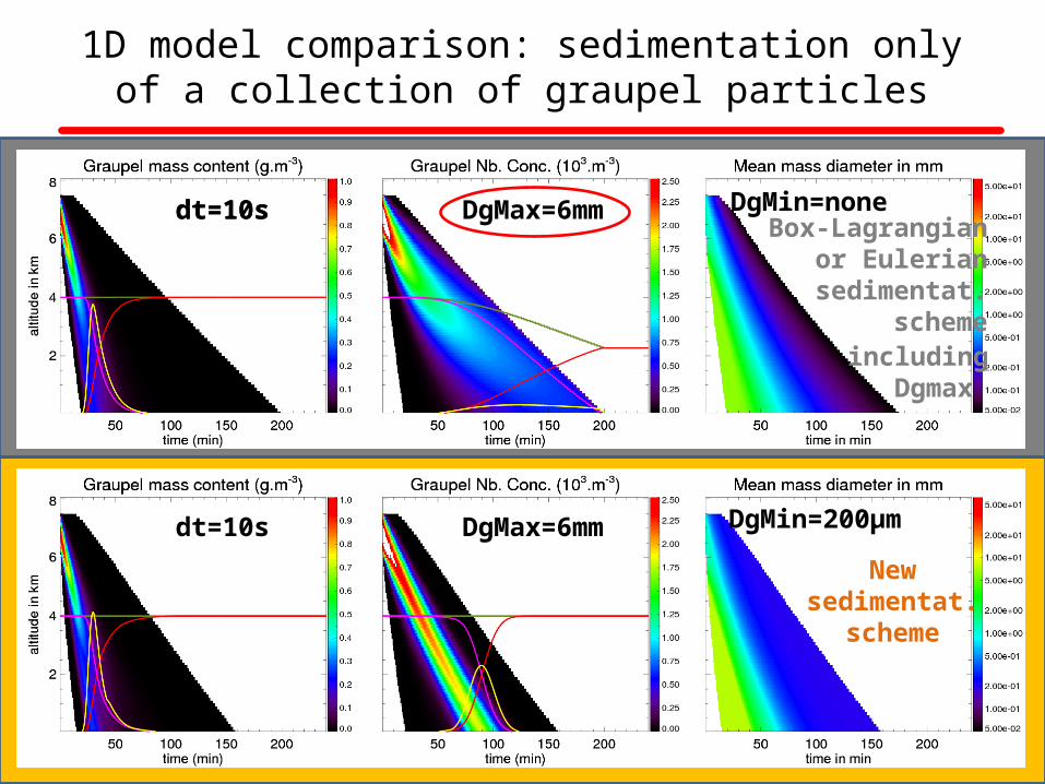
1D model comparison: sedimentation only of a collection of graupel particles
dt=10sdt=10s DgMax=6mm DgMin=noneBox-Lagrangian
or Euleriansedimentat.
schemeincluding
Dgmax
Newsedimentat.
scheme
DgMax=6mm DgMin=200μmdt=10s DgMax=6mm
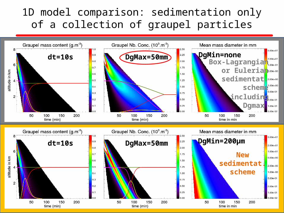
1D model comparison: sedimentation only of a collection of graupel particles
dt=10sdt=10s DgMax=50mm DgMin=noneBox-Lagrangian
or Euleriansedimentat.
scheme
Newsedimentat.
scheme
DgMin=200μm
includingDgmax
dt=10s DgMax=50mm
cdt=2min dt=3min dt=4min dt=8min
1D model comparison: sedimentation only of a collection of graupel particles
Newsedimentat.
schemeDgMax=6mm DgMin=200μm
dt=10s dt=30s dt=60s dt=90s
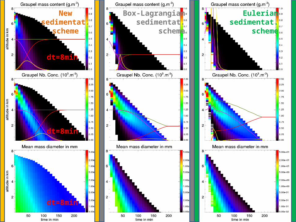
dt=8min
dt=8min
dt=8min
Box-Lagrangiansedimentat.
scheme
Newsedimentat.
scheme
Euleriansedimentat.
scheme
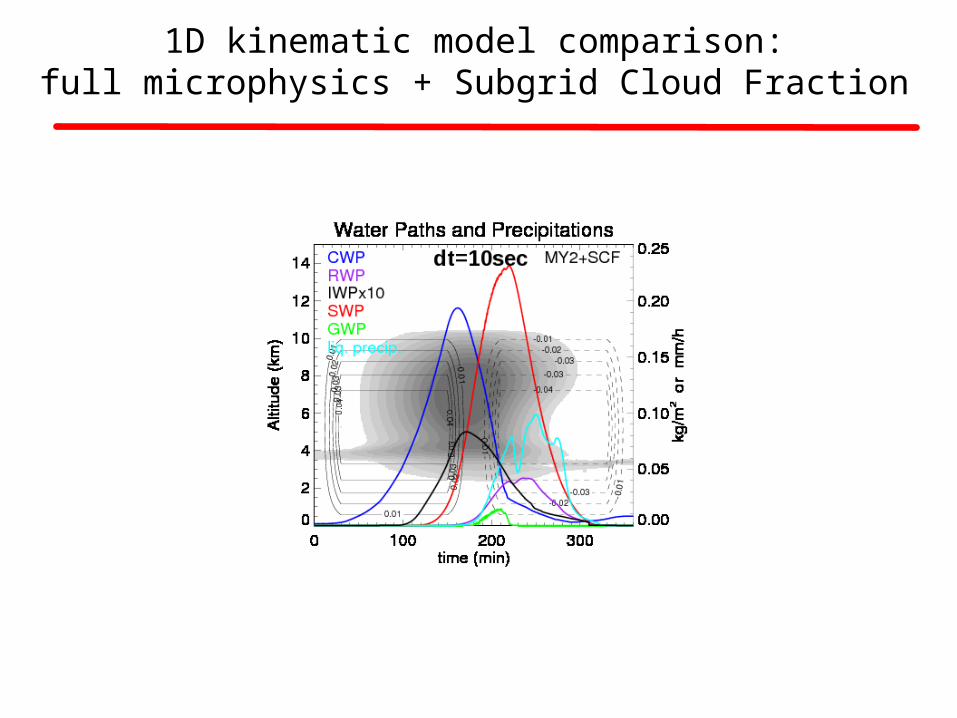
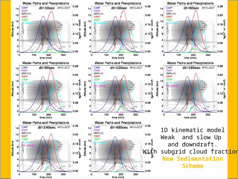
1D kinematic model comparison:full microphysics + Subgrid Cloud Fraction
c
1D kinematic modelWeak and slow Up
and downdraft.With subgrid cloud fraction.
New SedimentationScheme

c
1D kinematic modelWeak and slow Up
and downdraft.With subgrid cloud fraction.
EulerianSedimentation
Scheme

c
1D kinematic modelWeak and slow Up
and downdraft.With subgrid cloud fraction.
Box-LagrangianSedimentation
Scheme
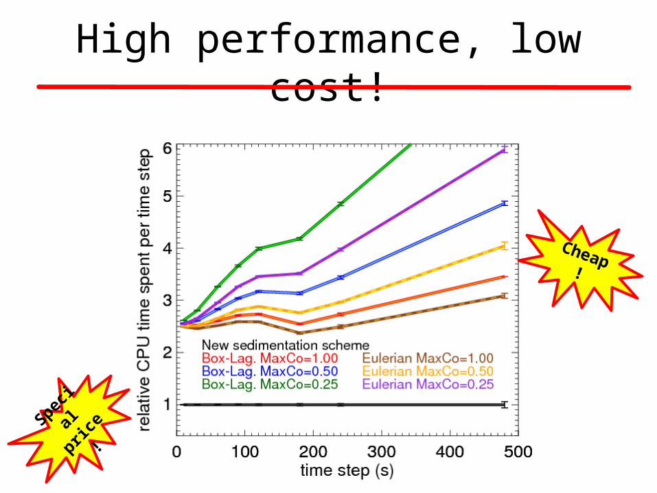
High performance, low cost!
Cheap!
Specia
lpric
e!
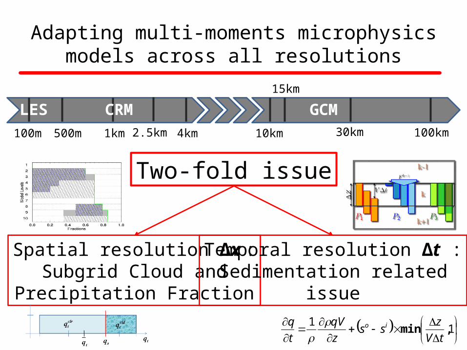
Adapting multi-moments microphysics models across all resolutions
Two-fold issue
GCM100m 500m 1km 4km 10km 30km 100km2.5km
15km
CRMLES
Spatial resolution ∆x :Subgrid Cloud and
Precipitation Fraction
Temporal resolution ∆t :Sedimentation related
issue
11
,mintV
zss
z
qV
t
q io
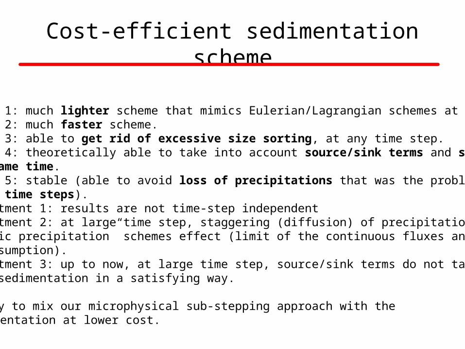
Cost-efficient sedimentation schemeConclusions:
• Advantage 1: much lighter scheme that mimics Eulerian/Lagrangian schemes at short ∆t.• Advantage 2: much faster scheme.• Advantage 3: able to get rid of excessive size sorting, at any time step.• Advantage 4: theoretically able to take into account source/sink terms and sedimentation at the same time.• Advantage 5: stable (able to avoid loss of precipitations that was the problem for long time steps).• Disappointment 1: results are not time-step independent• Disappointment 2: at large time step, staggering (diffusion) of precipitation close to “diagnostic precipitation” schemes effect (limit of the continuous fluxes and source/sink terms assumption).• Disappointment 3: up to now, at large time step, source/sink terms do not take into account sedimentation in a satisfying way.
→ Possibility to mix our microphysical sub-stepping approach with the new sedimentation at lower cost.
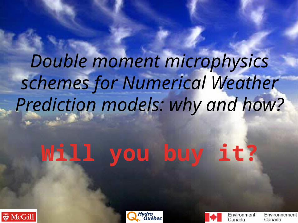
Double moment microphysics schemes for Numerical Weather
Prediction models: why and how?
Will you buy it?
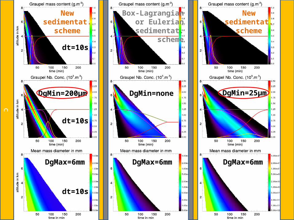
1D model comparison: sedimentation only of a collection of graupel particles
Box-Lagrangianor Eulerian
sedimentat.scheme
Newsedimentat.
scheme
Newsedimentat.
scheme
DgMin=200μm DgMin=25μm
DgMax=6mm DgMax=6mm DgMax=6mm
c
DgMin=none
dt=10s
dt=10s
dt=10s
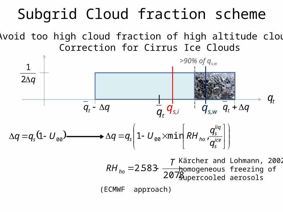
tq
Avoid too high cloud fraction of high altitude clouds:Correction for Cirrus Ice Clouds
q21
tq qq t qq t qs,i qs,w
>90% of qs,w
001 Uqq s
ices
liqs
hos q
qRHUqq ,min1 00
8.207583.2
TRHho
Kärcher and Lohmann, 2002homogeneous freezing of supercooled aerosols
Subgrid Cloud fraction scheme
(ECMWF approach)
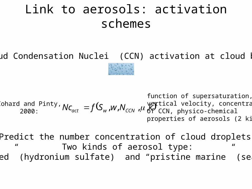
Link to aerosols: activation schemes
Cohard and Pinty,2000: kNwSfNc CCNwact ,,,,
function of supersaturation,vertical velocity, concentrationof CCN, physico-chemical properties of aerosols (2 kinds)
Cloud Condensation Nuclei (CCN) activation at cloud base:
Predict the number concentration of cloud droplets.Two kinds of aerosol type:
“polluted” (hydronium sulfate) and “pristine marine” (sea salt).
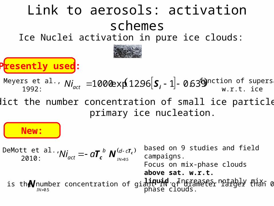
DeMott et al.,2010:
cTc NT cdb
act INaNi
5.0
based on 9 studies and field campaigns.Focus on mix-phase clouds above sat. w.r.t. liquid. Increases notably mix-phase clouds.
Meyers et al.,1992:
639.0196.12exp1000 iSactNi function of supersat.w.r.t. ice
Ice Nuclei activation in pure ice clouds:
Link to aerosols: activation schemes
Presently used:
New:
Predict the number concentration of small ice particles throughprimary ice nucleation.
5.0INN is the number concentration of giant IN of diameter larger than 0.5 microns