DOT/FAA/TC-18/6 Federal Aviation Administration William J. Hughes Technical Center Aviation Research Division Atlantic City International Airport New Jersey 08405

Probabilistic Design for Rotor Integrity October 2018 Final Report This document is available to the U.S. public through the National Technical Information Services (NTIS), Springfield, Virginia 22161. This document is also available from the Federal Aviation Administration William J. Hughes Technical Center at actlibrary.tc.faa.gov.

U.S. Department of Transportation Federal Aviation Administration

NOTICE

This document is disseminated under the sponsorship of the U.S. Department of Transportation in the interest of information exchange. The U.S. Government assumes no liability for the contents or use thereof. The U.S. Government does not endorse products or manufacturers. Trade or manufacturers’ names appear herein solely because they are considered essential to the objective of this report. The findings and conclusions in this report are those of the author(s) and do not necessarily represent the views of the funding agency. This document does not constitute FAA policy. Consult the FAA sponsoring organization listed on the Technical Documentation page as to its use. This report is available at the Federal Aviation Administration William J. Hughes Technical Center’s Full-Text Technical Reports page: actlibrary.tc.faa.gov in Adobe Acrobat portable document format (PDF).

Technical Report Documentation Page 1. Report No.

DOT/FAA/TC-18/6

2. Government Accession No. 3. Recipient's Catalog No.

4. Title and Subtitle

PROBABILISTIC DESIGN FOR ROTOR INTEGRITY

5. Report Date

October 2018

6. Performing Organization Code

7. Author(s)

R. Craig McClung* Jonathan P. Moody* Jonathan P. Dubke† Michael P. Enright* Simeon H. K. Fitch** Robert J. Maffeo†† Yi-Der Lee* Harry R. Millwater*** Michael E. McClure††† Wuwei Liang* Alonso D. Peralta††††

8. Performing Organization Report No.

18-11481

9. Performing Organization Name and Address

* Southwest Research Institute® † Rolls-Royce Corporation 6220 Culebra Road 2001 South Tibbs Avenue

San Antonio, TX 78238 Indianapolis, IN 46241 ** Elder Research, Inc. †† GE Aviation

300 West Main Street #301 1 Neumann Way Charlottesville, VA 229031 Cincinnati, OH 45215

*** University of Texas at San Antonio ††† Pratt & Whitney 6900 North Loop 1604 West 400 Main Street San Antonio, TX 78249 East Hartford, CT 06108

†††† Honeywell 111 South 34th Street

Phoenix, AZ 85072

10. Work Unit No. (TRAIS)

11. Contract or Grant No.

2005-G-005 12. Sponsoring Agency Name and Address

U.S. Department of Transportation Federal Aviation Administration FAA New England Regional Office 1200 District Ave Burlington, MA 01803

13. Type of Report and Period Covered

Final Report April 2005 – August 2011 14. Sponsoring Agency Code

AIR-6A1

15. Supplementary Notes

The FAA William J. Hughes Technical Center Aviation Research Division Technical Monitor was Joseph Wilson. 16. Abstract

This grant supported the efforts of the FAA to develop an enhanced life-management process, based on probabilistic damage-tolerance principles, to address the threat of material or manufacturing anomalies in high-energy rotating components of aircraft engines. Specific outcomes of the grant included enhanced predictive tool capability and supplementary material/anomaly behavior characterization and modeling. The efforts facilitate implementation of official advisory material for circular holes and support evolving methods for surface damage analysis of attachment slots and turned surfaces, while also developing improved analysis methods for inherent anomalies in all materials. Major research products included improved crack-growth life-prediction models and supporting experimental data, new methods for fracture mechanics characterization of cracks in rotors, automated methods for integrity and reliability assessment of actual components, and multiple new versions of the DARWIN® computer code for technology transfer to industry and the FAA. 17. Key Words

Aircraft gas turbine engines, Disks, Rotors, Low cycle fatigue, Fracture mechanics, Probabilistic damage tolerance, Risk assessment, Surface damage, DARWIN

18. Distribution Statement

This document is available to the U.S. public through the National Technical Information Service (NTIS), Springfield, Virginia 22161.

19. Security Classif. (of this report)

Unclassified

20. Security Classif. (of this page)

Unclassified

21. No. of Pages

312

22. Price

Form DOT F 1700.7 (8-72) Reproduction of completed page authorized

iii

ACKNOWLEDGEMENTS

Successful completion of this large, multidisciplinary research project would not have been possible without the significant contributions and assistance of many different people. Some are named as authors in this report, and many others deserve special mention.

Special appreciation is extended to the FAA employees and consultants who provided sustained support, encouragement, and guidance throughout the project. Heartfelt thanks goes to Tim Mouzakis of the Engine and Propeller Directorate in the New England Regional Office, Joe Wilson of the William J. Hughes Technical Center, and FAA consultants Jon Bartos and Nick Provenzano.

The entire project was motivated and guided by the Rotor Integrity Sub-Committee of the Aerospace Industries Association, led by current chairman Michael Gorelik and previous chairman Bill Knowles, both from Honeywell.

Direct leadership was provided by the industry Steering Committee comprising representatives from the four partner companies: GE Aviation (GEA), Honeywell, Pratt & Whitney (P&W), and Rolls-Royce® Corporation (RRC). Current members are chair Jon Dubke (RRC), Mike McClure (P&W), Alonso Peralta (Honeywell), and Bob Maffeo (GEA). Previous members during the term of this program include former chair Darryl Lehmann and Johnny Adamson (both from P&W), Jon Tschopp (GEA), and Ahsan Jameel and Michael Gorelik (both from Honeywell).

The development of high-temperature crack-growth methods was guided by an informal advisory team comprised of Bob Van Stone (formerly GEA), Barney Lawless (GEA), Rick Pettit (formerly P&W), Fashang Ma (P&W), Tom Cook and David Mills (RRC), and Youri Lenets and Terry Richardson (Honeywell).

Barney Lawless and Bob Van Stone led the time-dependent crack-growth program at GEA, with additional methods help from Sue Gilbert. Fashang Ma led the investigation of alternative analysis methods for time-dependent crack growth at P&W.

James Hartman and Gil Mora led fatigue crack-growth testing activities at Honeywell.

Yi-Der Lee (Southwest Research Institute®, SwRI®) performed all development activities for the Flight_Life fracture mechanics module, including generating all stress intensity factor solutions.

Craig McClung and Vikram Bhamidipati (both from SwRI) performed the small-crack study. Special appreciation is extended to Mike Caton (Air Force Research Laboratory, AFRL), Sushant Jha (AFRL), Youri Lenets (Honeywell), Jack Telesman (NASA Glenn Research Center, GRC), and Jim Newman (Mississippi State University) for generously providing their data from other projects and answering many questions. Additional financial support for analysis of the U-720 data was provided by NASA GRC through Contract No. NNC08CB06C (Jack Telesman, project monitor).

DARWIN development was led by Michael Enright (SwRI), with substantial support from Wuwei Liang (SwRI) and Luc Huyse (formerly SwRI). Jonathan Moody (SwRI) and Chris Waldhart (formerly SwRI) led DARWIN testing and validation activities. Simeon Fitch, Ben Guseman, and

iv

Ben Hocking (all Elder Research, formerly known as Mustard Seed Software) performed all graphical user interface development for DARWIN.

Steve Schrantz and Bob McClain (both GEA) provided assistance with finite element method model translation.

Harry Millwater and his students and colleagues provided additional DARWIN support at the University of Texas at San Antonio. Those contributors included Jonathan Moody, Wesley Osborn, Faiyazmehadi Momin, Gulshan Singh, and Tony Castaldo.

The partner companies provided extensive evaluation and testing of new DARWIN releases throughout the program. Key contributors included Mike Hartle (GEA); Alonso Peralta (Honeywell) and Ahsan Jameel (formerly Honeywell); Jon Dubke, Jason Baker, Justin Gilman, and Doug Olsen (all RRC); and Darryl Lehmann and Mike McClure (both P&W).

Birdie Matthews (SwRI) provided superlative clerical assistance in preparing this large final report. Gerry Leverant (SwRI consultant) is thanked for his careful peer review of the report.

v

TABLE OF CONTENTS

Page

EXECUTIVE SUMMARY xvi 

1. INTRODUCTION 1 

1.1 Background 1 1.2 Organization of Research 5

2. ADVANCED DAMAGE TOLERANCE METHODS 6 

2.1 Time-Dependent Fatigue Crack Growth 6

2.1.1 Superposition Models 6 2.1.2 Retardation Models 10

2.2 Non-Isothermal Fatigue Crack Growth 11

2.2.1 Use of Isothermal Fatigue Crack Growth Properties for Non-Isothermal Cycling 11 

2.2.2 Time-Dependent Shakedown During Non-Isothermal Crack Growth 12

2.3 Small Fatigue Cracks 12 2.4 Nickel Anomaly Fatigue Testing 14 2.5 Benchmark Fatigue Crack Growth Data 15

3. ADVANCED FRACTURE ANALYSIS 16 

3.1 New and Enhanced Stress Intensity Factor Solutions 16

3.1.1 New Bivariant SIF Solution for Semi-Elliptical Surface Crack in Plate 16 3.1.2 Extension of Validity Limits for Univariant SIF for Semi-Elliptical

Surface Crack in Plate 17 3.1.3 Improved Integration Methods for Bivariant SIF Solutions 18 3.1.4 Pre-Integration Methods for Univariant SIF Solutions 18 3.1.5 New Univariant SIF Solution for Through Crack in Variable Thickness

Plate 18 3.1.6 New Bivariant and Univariant SIF Solutions for Elliptical Embedded

Crack in Plate 21 3.1.7 Enhanced Bivariant SIF Solution for Corner Crack in Plate with Non-

Normal Corners 21 3.1.8 Integration of New Univariant SIF Solution for Corner Crack in Plate 22 3.1.9 Revisions to Available Crack Model Solutions in DARWIN 22

3.2 Bivariant Shakedown Module 23 

vi

3.3 Facilities for User-Supplied SIF Tables 26 3.4 Alternative Stress Ratio Model Based on Stress Level Sensitivity 27 3.5 HCF Threshold Check 28

4. ADVANCED PROBABILISTIC METHODS 28 

4.1 Computing Life for a Specified Probability of Fracture 28 4.2 Approximate Risk Contours 30

5. ADVANCED ZONING CAPABILITIES 31 

5.1 Treatment of Stress Concentrations in 2D Models 32 5.2 Surface Zoning 35

5.2.1 Risk Assessment for Surface Damage of 2D Models 35 5.2.2 Surface Area of Blade Slots 36

5.3 Auto-Modeling 38

5.3.1 Automatic Construction of Fracture Models 38 5.3.2 Life Contours 44 5.3.3 Autozoning 46 5.3.4 GUI Redesign to Support Autozoning 47

6. GENERAL DARWIN ENHANCEMENTS 49 

6.1 Direct Support for Implementation of Advisory Circulars 50

6.1.1 Special Analysis Modes for Certification Assessments 50 6.1.2 Advisory Circular 33.70-2 for Hole Features 51

6.2 FE2NEU Translator 55 6.3 Improvements for General Inherent Anomalies 59 6.4 Speed and Accuracy Improvements 59

6.4.1 Parallel Processing 60 6.4.2 Enhanced Restart Algorithm 62 6.4.3 Treatment of Shakedown with Stress Scatter 63 6.4.4 Crack Growth Life Interpolation Enhancement 63 6.4.5 Enhanced Mesh Generation Algorithm 64 6.4.6 Computational Speed Improvement for Critical Anomaly Size

Computation 65 6.4.7 Accuracy Improvement for LAF Method 66 6.4.8 Computational Speed Improvements Associated with New Fortran

Compiler 66 6.4.9 Computational Speed Improvements Due to Representation of Text

Strings 66

vii

6.5 Stress Processing Enhancements 66

6.5.1 Enhanced Finite Element Search Algorithm 67 6.5.2 Parsing Data from Stress Results Files 67 6.5.3 Stress Gradient Search Algorithm Enhancement 67 6.5.4 Multiple Load Steps for 3D Models 68 6.5.5 Mission Scaling Factor Enhancements 68

6.6 Database and File Management Enhancements 69

6.6.1 XML Input File/Text Editor 69 6.6.2 Managing Large Files 70 6.6.3 Additional Output for Deterministic Crack Growth Assessments 71 6.6.4 Verification Checks And Keywords 74

6.7 User Interface Enhancements 74

6.7.1 Filtering of GUI Warning Messages 74 6.7.2 GUI Display of Optional Features 76

7. DARWIN TESTING AND EVALUATION 76 

7.1 DARWIN Code Releases 77

7.1.1 DARWIN 6.0 77 7.1.2 DARWIN 6.1 77 7.1.3 DARWIN 7.0 77 7.1.4 DARWIN 7.1 78 7.1.5 DARWIN 7.2 78

7.2 DARWIN Internal Verification Testing 79

7.2.1 Modular Code Development and Verification 79 7.2.2 Incremental Code Releases 79 7.2.3 Automated Verification Testing 80

7.3 OEM Evaluation 81

7.3.1 Quantitative Verification 81 7.3.2 Qualitative Evaluation 81 7.3.3 OEM Review Comments 81

8. TECHNOLOGY TRANSFER 82 

8.1 Progress Reports and Review Meetings 82 8.2 Conference Presentations and Journal Articles 82 

viii

8.3 Darwin Commercial Licensing 82 8.4 Technology Transfer to Other U.S. Government Agencies 83 8.5 Darwin Spin-Off Projects 83

8.5.1 Enhanced Life Prediction Technology for Engine Rotor Life

Extension 84 8.5.2 Extension of Bimodal Failure Distribution Concepts 84 8.5.3 Integrated Processing and Probabilistic Lifing Models for Superalloy

Turbine Disks 85 8.5.4 Three-Dimensional Crack Growth Life Prediction for Probabilistic

Risk Analysis of Turbine Engine Metallic Components 85 8.5.5 Probabilistic Fretting Fatigue Assessment of Gas Turbine Engine

Disks 86 8.5.6 Probabilistic Mission Analysis for Assessment of Alternative Fuels in

Turbine Engines 86 8.5.7 Life and Reliability Prediction for Turbopropulsion Systems 86 8.5.8 Lifing Technology for Powder Metallurgy Alloys 87 8.5.9 Hot Corrosion of Nickel-Based Turbine Disks 87 8.5.10 Extension of DARWIN for Continued Airworthiness Assessment 88

9. SUMMARY 88 

10. REFERENCES 91

APPENDICES

A—TIME-DEPENDENT AND OVERPEAK RETARDATION CRACK GROWTH BEHAVIOR  

B—A NEW ANALYSIS METHOD FOR TIME-DEPENDENT CRACK GROWTH  

C—ANALYTICAL MODELS FOR THERMO-MECHANICAL FATIGUE (TMF) WITH HOT COMPRESSIVE CYCLES  

D—AN INVESTIGATION OF SMALL-CRACK EFFECTS IN VARIOUS AIRCRAFT ENGINE ROTOR MATERIALS

E—NICKEL ANOMALY FATIGUE TESTING FBENCHMARK FATIGUE CRACK GROWTH TESTING  

G—DEVELOPMENT OF NEW AND ENHANCED STRESS INTENSITY FACTOR SOLUTIONS  

H—ADAPTIVE RISK REFINEMENT  

I—LIST OF PUBLICATIONS AND PRESENTATIONS DURING “PROBABILISTIC DESIGN FOR ROTOR INTEGRITY” GRANT  

ix

LIST OF FIGURES

Figure Page

1 The broad vision for an enhanced rotor life management process based on damage tolerance 4 

2 Static crack growth test data for IN-718 at 1100F and 1200F with regression fits to a simple power law equation 8 

3 Static crack growth curves interpolated at intermediate temperatures between two bounding temperatures at 1100F and 1200F using arrhenius function to represent the coefficients for the power law relationship 8 

4 Experimental versus predicted specimen lives using a superposition model or a cyclic crack growth model 10 

5 Focused ion beam notch with surface crack 14 

6 Schematic diagram (not to scale) showing multiple FIB Notches in a flat specimen 14 

7 Schematic for surface crack configuration of SC19 17 

8   Applicable cracked configuration for TC15 A through-thickness crack at the edge of a variable-thickness plate: (a) Thickness variation across the plate section in symmetry to the mid-plane of the plate, and (b) Remote ends subjected to loading normal to the crack 19 

9 Illustration of a new GUI capability that enables the analyst to interactively create and edit fracture models for edge through cracks in plates of non-uniform thickness (TC15): (a) Finite element model with non-uniform width features, (b) Enlarged view of non-uniform width features, (c) TC15 fracture model superimposed on finite element geometry in DARWIN GUI, and (d) TC15 fracture model coordinates and associated stress contour results 20 

10 Notations used for the embedded crack configuration in a rectangular section 21 

11 Illustration of new GUI capability for bivariant corner cracks (CC09) at non-normal corners: (a) Placement of CC09 at a non-normal corner in the finite element model, and (b) Adjustment of CC09 corner angle to match the finite element geometry 22 

12 Comparison of predicted elastic-plastic stress results from bivariant shakedown module with FEA results for MATL-A: (a) Stress variation from elastic FEA, (b) Stress variation from elastic-plastic FEA, and (c) Predicted elastic-plastic stress variation from shakedown module 25 

13 Comparison of predicted elastic-plastic stress results from bivariant shakedown module with FEA results for MATL-B: (a) Stress variation from elastic FEA, (b) Stress variation from elastic-plastic FEA, and (c) Predicted elastic-plastic stress variation from shakedown module 26 

14 GUI window for zone editor showing new capability for user-supplied K tables 27 

15 GUI screens for new HCF threshold check capability in DARWIN 28 

x

16 User specification of a target Pf value in the DARWIN GUI to activate the “life for a specified probability of fracture” capability 29 

17 Illustration of the DARWIN “life for a specified probability of fracture” capability. Life values are displayed at the locations where risk curves intersect the user- specified probability of fracture value (indicated in the as a red horizontal line) 30 

18 Conceptual model for predicting approximate risk contour values in which an anomaly distribution is transformed into a crack growth life distribution via life contours associated with key anomaly sizes 31 

19 Illustration of disk cross sections influenced by stress concentration (Kt) effects: (a) Axial view of disk indicating location of slices, (b) Cross-section through hole and associated Kt region, and (c) Cross-section without holes (without Kt) 32 

20 The Kt feature is enabled by the analyst in the DARWIN “setup” menu. It is currently limited to the general inherent analysis mode 33 

21 Interpolation of stress values at a point located within a virtually-filled hole 33 

22 Illustration of a “Kt-affected” zone at the surface of a hole: (a) Cross-section through hole including effect of Kt (with Kt), and (b) Cross-section without holes (without Kt). Note that the zone volume, crack location, and plate dimensions may differ for the two cross-sections 34 

23 A DARWIN capability was implemented for assessment of turned surfaces near stress concentrations 35 

24 Illustration of the new DARWIN 2D surface damage analysis mode that was developed to assess risk associated with 2D turned surfaces 36 

25 A new capability to quantify the surface area of blade slots in 3D finite element models was implemented in DARWIN. User selection of (a) a Single surface region, and (b) Multiple surface regions 37 

26 The new blade slot area quantification capability includes controls to specify the finite element faces that are included in the assessment 38 

27 Example of plate model for surface crack where orientation is defined by tangency to component boundary 40 

28 (a) Example of plate model for embedded crack where orientation is defined by nearby component boundary; (b) Example of plate model for embedded crack where orientation is defined by significant stress gradient 41 

29 Schematic illustration of plate sizing algorithm 42 

30 Example of plate model for surface crack on non-straight boundary 43 

31 (a) Hoop stress contour plot for part of an axisymmetric ring disk geometry; (b) Corresponding life contour plot 44 

32 (a) Hoop stress contour plot for part of an axisymmetric impeller geometry; (b) Corresponding life contour plot 45 

xi

33 Convergence of disk risk with increasing number of zones using the automated risk refinement approach 47 

34 The user interface was enhanced to enable the analyst to assign component properties directly to finite elements rather than zones 48 

35 DARWIN was enhanced to identify the regions with unique properties 48 

36 DARWIN includes a capability to convert property regions into zones for use in manual zoning 49 

37 DARWIN was enhanced to provide risk contour plots for improved visualization of risk compared to risk contribution factor plots. (a) Example risk contribution factor plot, and (b) Example risk contour plot 49 

38 Redefined DARWIN analysis modes: (a) “General” analysis mode, which provides access to all of the DARWIN capabilities and (b) “FAA certification” analysis mode, restricted to the DARWIN anomaly types and analysis methods currently addressed by FAA advisory circulars 33.14-1 or 33.70-2 50 

39 DARWIN GUI screens for user specification of manufacturing process credits 52 

40 FAA hole feature surface damage report form implemented in DARWIN 7.0 54 

41 Overview of FE2NEU finite element results translator 55 

42 Examples of reduction in the time required to convert an ANSYS file to the DARWIN neutral file format using FE2NEU versus ANS2NEU 56 

43 An example ANSYS named component definition file 57 

44 The finite element filtering process using ANSYS named components 58 

45 Selection of named components filter in FE2NEU 58 

46 Two configurations were identified to model the area of a general inherent anomaly detected using available inspection techniques: (1) Intersection and (2) Projection 59 

47 The computational efficiency associated with the DARWIN parallel processing capability is dependent on the number of processors (CPUs) that are allocated to it 61 

48 DARWIN GUI screen illustrating user specification of the number of processors (CPUs) to be applied to parallel processing computations 61 

49 Schematic illustration of stress scatter distribution and yield stress ( ) 63 

50 Flight_life results based on optimal cycle increments and the interpolated results at user-specified print intervals 64 

51 Mesh discontinuities introduced by the previous DARWIN mesh generation algorithm 65 

52 Illustrative example of onion-skin mesh generation: (a) Unrefined mesh, (b) Previous mesh generation algorithm (DARWIN 6.1), and (c) New mesh generation algorithm (DARWIN 7.0) 65 

53 Schematic illustration of point containment test algorithm 68 

y

xii

54 “Absolute” mission scaling mode implemented in DARWIN GUI 68 

55 XML editor implemented in DARWIN that enables the user to view and edit XML- based input files 70 

56 DARWIN output verbosity control settings 71 

57 DARWIN output verbosity predefined output modes 71 

58 A sample DARWIN deterministic output data file (NOTE: the index numbers “1, 2, 3, 4” following “Kmax” indicate the respective crack tips) 74 

59 DARWIN GUI capability allowing user-specified filtering of warning messages: (a) Activation of the filtering capability, and (b) User interface for specification of filtered messages 75 

60 DARWIN GUI capability allowing the user to view active optional features available in DARWIN 76 

61 Schematic diagram for new Fortran automated verification process 80 

 

xiii

LIST OF TABLES

Table Page

1 Summary of manufacturing process controls and associated credit factors 51 

2 Finite element types supported by FE2NEU 55 

3 File access operations associated with DARWIN 6.0 and 6.1 restart algorithms 62 

4 Summary of deterministic output variables available in DARWIN 72 

xiv

LIST OF ACRONYMS

2D Two-dimensional 2mdw 2-minute dwell 3D Three-dimensional AC Advisory Circular AFRL Air Force Research Laboratory AIA Aerospace Industries Association ARRM Adaptive Risk Refinement Methodology ASC Aeronautical Systems Center BE Boundary element BH Bolt hole CAAM Continued Airworthiness Assessment Methodologies CAPRI Contact Analysis for Profiles of Random Indentors CBM+ Condition Based Maintenance Plus CC(T) Corner crack tension CPCA Compression precracking – constant amplitude CPLR Compression precracking – load reduction CPM Cycles per minute CPU Central processing unit C(T) Compact tension DARWIN Design Assessment of Reliability With INspection DEN Double-edge notch DUS&T Dual-Use Science and Technology EDM Electro-discharge machined EH El Haddad ERLE Engine Rotor Life Extension FAC Fracture Analysis Consultants FCG Fatigue crack growth FE Finite element FEA Finite element analysis FEM Finite element method FEST-Swing Fixtures for Easy Software Testing FIB Focused ion beam GEA General Electric Aviation GRC NASA Glenn Research Center GUI Graphical user interface HA Hard alpha HCF High-cycle fatigue LAF Life approximation function LCF Low-cycle fatigue LR Load reduction LSG Low stress grinding M(T) Middle-crack tension NAVAIR Naval Air Systems Command OEM Original equipment manufacturer OP Overpeak

xv

P&W Pratt & Whitney PDRI Probabilistic Design for Rotor Integrity PWF Point weight function RISC Rotor Integrity Sub-Committee RI Reduction index RRC Rolls-Royce Corporation SBIR Small Business Innovative Research SC Surface crack SC(T) Surface crack tension SF Surface flaw SFTC Scientific Forming Technologies Corporation SGBEM-FEM Symmetric Galerkin Boundary Element Method—Finite Element Method SIF Stress intensity factor SSY Small-scale yielding SwRI Southwest Research Institute TMF Thermo-mechanical fatigue TRMD Turbine Rotor Material Design USAF United States Air Force UT Ultrasonic WF Weight function XML Extensible Markup Language

xvi

EXECUTIVE SUMMARY

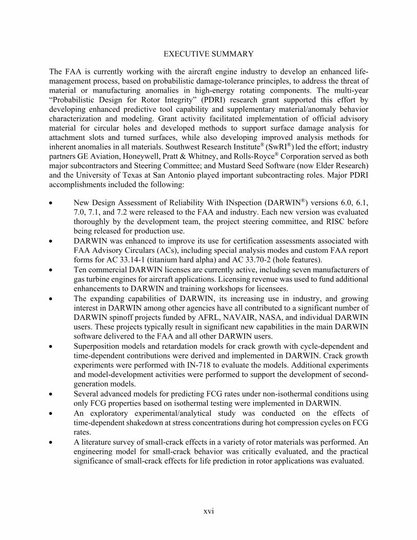
The FAA is currently working with the aircraft engine industry to develop an enhanced life-management process, based on probabilistic damage-tolerance principles, to address the threat of material or manufacturing anomalies in high-energy rotating components. The multi-year “Probabilistic Design for Rotor Integrity” (PDRI) research grant supported this effort by developing enhanced predictive tool capability and supplementary material/anomaly behavior characterization and modeling. Grant activity facilitated implementation of official advisory material for circular holes and developed methods to support surface damage analysis for attachment slots and turned surfaces, while also developing improved analysis methods for inherent anomalies in all materials. Southwest Research Institute® (SwRI®) led the effort; industry partners GE Aviation, Honeywell, Pratt & Whitney, and Rolls-Royce® Corporation served as both major subcontractors and Steering Committee; and Mustard Seed Software (now Elder Research) and the University of Texas at San Antonio played important subcontracting roles. Major PDRI accomplishments included the following:

New Design Assessment of Reliability With INspection (DARWIN®) versions 6.0, 6.1, 7.0, 7.1, and 7.2 were released to the FAA and industry. Each new version was evaluated thoroughly by the development team, the project steering committee, and RISC before being released for production use.

DARWIN was enhanced to improve its use for certification assessments associated with FAA Advisory Circulars (ACs), including special analysis modes and custom FAA report forms for AC 33.14-1 (titanium hard alpha) and AC 33.70-2 (hole features). 

Ten commercial DARWIN licenses are currently active, including seven manufacturers of gas turbine engines for aircraft applications. Licensing revenue was used to fund additional enhancements to DARWIN and training workshops for licensees.

The expanding capabilities of DARWIN, its increasing use in industry, and growing interest in DARWIN among other agencies have all contributed to a significant number of DARWIN spinoff projects funded by AFRL, NAVAIR, NASA, and individual DARWIN users. These projects typically result in significant new capabilities in the main DARWIN software delivered to the FAA and all other DARWIN users. 

Superposition models and retardation models for crack growth with cycle-dependent and time-dependent contributions were derived and implemented in DARWIN. Crack growth experiments were performed with IN-718 to evaluate the models. Additional experiments and model-development activities were performed to support the development of second-generation models.

Several advanced models for predicting FCG rates under non-isothermal conditions using only FCG properties based on isothermal testing were implemented in DARWIN.

An exploratory experimental/analytical study was conducted on the effects of time-dependent shakedown at stress concentrations during hot compression cycles on FCG rates.

A literature survey of small-crack effects in a variety of rotor materials was performed. An engineering model for small-crack behavior was critically evaluated, and the practical significance of small-crack effects for life prediction in rotor applications was evaluated.

xvii

An experimental investigation was conducted to characterize the impact of naturally occurring material anomalies on the fatigue performance of rotor-grade conventional nickel material. Double-melted IN-718 material containing significant anomalies had previously been forged and heat treated to rotor specification. Two tests of fatigue specimens containing embedded anomalies indicated that a significant fraction of the total fatigue life was associated with crack formation at a known anomaly.

FCG data were generated with different specimen geometries for a fine-grained delta-processed IN-718 alloy to facilitate the validation of DARWIN stress intensity factor (SIF) solutions and related FCG algorithms.

New or significantly improved univariant or bivariant weight function SIF solutions were developed, verified, and implemented in DARWIN for an offset semi-elliptical surface crack (SC19 and SC17), an offset elliptical embedded crack (EC04 and EC05), a through-thickness edge crack in a variable-thickness plate (TC15), and a quarter-elliptical corner crack in a plate (CC09) with corner angles of 905. Several enhancements were also derived and implemented to significantly improve the computational efficiency of these and other DARWIN SIF solutions.

A new shakedown module for bivariant stressing was developed and implemented in DARWIN. The method converts a user-provided linear elastic finite element (FE) solution into an elastic-plastic solution.

A new capability was implemented that allows importing an externally generated table of SIF values into DARWIN for use in life and fracture risk computations.

A new capability was implemented in DARWIN that allows the user to include the influence of vibratory (high-cycle fatigue) stress values on fracture risk computations.

An algorithm was developed and implemented in DARWIN to predict the number of flight cycles associated with a user-specified probability of fracture (target risk) value.

A DARWIN capability to address stress concentration factor gradients in two-dimensional (2D) axisymmetric models was developed to support inherent anomaly assessments and surface damage on turned surfaces.

A new surface-zoning capability for 2D axisymmetric FE models was implemented in DARWIN to provide support for risk assessment of turned surfaces. A new capability to characterize surface area at blade slots was also developed to support RISC activities.

Automated modeling capabilities were implemented in DARWIN to reduce cost and human-factors variability in the current analysis process. These capabilities include automatic construction of fracture mechanics models, life contours, and autozoning.

A new FE2NEU FE results translator was developed to convert ANSYS and ABAQUS results to the neutral file format required by DARWIN with expanded capabilities and improved computational efficiency.

A new parallel-processing capability was implemented in DARWIN that automatically distributes the risk-assessment code computations to multiple processors on a single computer using the OpenMP® approach. Testing confirmed substantial reductions in computation time.

Several significant enhancements were implemented to DARWIN software verification procedures.

A number of other general DARWIN enhancements addressed computational efficiency and accuracy as well as database and file management for large application problems.

1

1. INTRODUCTION

1.1 BACKGROUND

The traditional design practice for high-energy aircraft gas turbine rotors, the so-called “safe-life” method, implicitly assumes that all material or manufacturing conditions that may influence the fatigue life of a rotor have been captured in laboratory coupon and full-scale component fatigue testing. This methodology provides a structured approach for design and life management that ensures high levels of safety. However, industry experience has shown that certain material and manufacturing anomalies can potentially degrade the structural integrity of high-energy rotors. These anomalies occur very rarely and, therefore, are not typically present in laboratory test articles. However, on those rare occasions when anomalies are present in manufactured products in service, they represent a significant departure from the assumed nominal conditions, and they can result in such incidents as the Sioux City accident in 1989.

As a result of Sioux City, the FAA requested that industry, through the Aerospace Industries Association (AIA) Rotor Integrity Sub-Committee (RISC), review available techniques to determine whether a damage-tolerance approach could be introduced to produce a reduction in the rate of uncontained rotor events. The industry working group concluded that additional enhancements to the conventional rotor life management methodology could be developed that explicitly addressed anomalous conditions. During the development of this probabilistic damage tolerance approach, it became apparent to RISC that the capabilities and effectiveness of the emerging technology could be significantly enhanced by further research and development. In early 1995, Southwest Research Institute® (SwRI®), in partnership with four major U.S. engine manufacturers and with guidance from RISC, proposed a multiple-year R&D program and was awarded an FAA grant to address identified shortfalls in technology and data. This program, titled “Turbine Rotor Material Design” (TRMD), developed enhanced predictive tool capability and supplementary material/anomaly behavior characterization and modeling with a particular focus on hard alpha (HA) anomalies in titanium rotors.

One of the key outcomes of this work was a probabilistic damage-tolerance computer code called DARWIN® (Design Assessment of Reliability With INspection). DARWIN integrates finite element models (FEMs) and stress analysis results, fracture mechanics models for low-cycle fatigue, material anomaly data, probability of crack detection by nondestructive inspection, and uncertain inspection schedules with a user-friendly graphical user interface (GUI) to determine the probability-of-fracture of a rotor disk as a function of operating cycles with and without inspections. Other major accomplishments under the TRMD grant included the following [1]:

Generation of fatigue crack growth (FCG) data in vacuum (needed to characterize subsurface crack growth) for three titanium rotor alloys [2]

Experimental and analytical characterization of the constitutive and damage properties of bulk titanium HA [3,4]

Experimental characterization of HA cracking in titanium alloy matrix material under monotonic and cyclic loading [5]

Development of a forging microcode capable of predicting the fracture and change of location and shape of HA during reduction from ingot to billet and from billet to final forged shape, and forging experiments to validate the microcode

2

Development of advanced probabilistic methods for risk assessment of components with rare inherent material anomalies [6]

Three versions of an integrated probabilistic damage-tolerance design code (DARWIN) with a user-friendly GUI [7] and an integrated fracture mechanics module (Flight_Life)

Verification and validation of DARWIN against industry software and experience

An incident in Pensacola, Florida in 1996 called special attention to surface anomalies induced during manufacturing. With guidance from the FAA, RISC began to apply and extend the insights and methods developed for inherent material anomalies in titanium rotors to the broader problem of induced surface anomalies in all rotor materials. SwRI, in continuing collaboration with the industry, proposed and was awarded a second FAA grant (“Turbine Rotor Material Design – Phase II”). This project began to address the surface anomaly challenge while completing the titanium HA work. Major accomplishments of TRMD-II included the following [8]:

A mathematical model and computer code to describe the diffusion of nitrogen or oxygen in titanium from an inclusion during metal forming and heat treatment

Detailed NDE and metallography of forgings with known HA anomalies to validate the HA forging microcode

Analytical characterization of the nitrogen contents, temperatures, strain rates, and orientations associated with cracking of HA anomalies during the forging operation

Experimental investigations of the effects of oxygen on tensile, fatigue, and dwell-fatigue behavior of Ti-17

Experimental measurement of the coefficient of thermal expansion of bulk HA with different nitrogen contents

Evaluation of the potential effects of thermally induced residual stresses on fatigue crack initiation and growth at HA inclusions [9]

Spin pit tests and coupon fatigue tests, including periodic nondestructive inspection, along with post-test fractography and metallography, performed with material from the TRMD-Phase I forgings containing natural and synthetic HA anomalies

Vacuum FCG data generated at representative temperatures and stress ratios for one titanium rotor alloy (coarse-grained Ti-6-2-4-2), two nickel rotor alloys (IN-718 and Waspaloy), and one powder metallurgy nickel alloy (Udimet 720)

Thermo-mechanical FCG data for IN-718 generated with diagnostic stress-temperature histories, demonstrating that stress rainflow analysis methods using isothermal data from the temperature at the maximum stress time point exhibit a nonconservative bias

A new weight function (WF) stress intensity factor (SIF) formulation that accommodates general bivariant stress distributions on the crack plane [10]

Highly accurate new WF SIF solutions for select crack geometries under univariant and bivariant stressing using state-of-the-art three-dimensional (3D) boundary-element analysis to generate the reference solutions [10,11,12]

A comprehensive literature survey on the stability and significance of residual stresses in fatigue [13]

Advanced probabilistic methods to improve the efficiency and accuracy of risk assessment computations, including an importance sampling technique and associated confidence bounds that significantly improve the risk computation speed compared to Monte Carlo simulation [14,15,16]

3

A method to assign Monte Carlo samples to zones based on relative risk that dramatically reduces the total number of samples (and computation time) required to predict risk for a specified level of accuracy [16,17]

A sophisticated 3D GUI that enables the user to load and visualize a fully 3D FE model and stress results, select a surface crack (SC) location, slice the 3D model along the principal stress plane at that location, re-mesh the slice to create a two-dimensional (2D) stress model, build a 2D fracture mechanics model on the cut plane, and extract the necessary input for the 2D fracture mechanics life calculation [10]

New DARWIN versions 4.x, 5.x, and 6.0 developed to implement these and other technology advances in a computer program that can easily be used by engine companies for design and certification purposes, and verification and validation of each DARWIN version by comparison with engine company software and experience

An infrastructure for formal software configuration management, code licensing and distribution, and user support, so that engine companies can employ DARWIN for official FAA and company purposes

The broad RISC vision for enhanced life management of high-energy rotors is summarized in figure 1. This vision embraces both inherent anomalies introduced during production of the rotor materials and induced surface anomalies introduced during manufacturing or maintenance of the rotors themselves. All rotor materials are addressed—titanium alloys, conventional cast and wrought nickel alloys, and advanced nickel alloys employing powder metallurgy technologies. The red check mark adjacent to the “titanium hard alpha” box indicates that the methods and supporting technologies to address that threat were developed and then formally defined in FAA AC 33.14. More recently, RISC activities have been primarily focused on anomalies induced during manufacturing, starting with circular holes, and then moving on to begin addressing attachment slots and smooth surfaces. The red check mark adjacent to the “circular hole” box denotes the development and release of FAA AC 33.70-2. Some preparatory work has also been underway in RISC to address inherent anomalies in nickel alloys.

4

Figure 1. The broad vision for an enhanced rotor life-management process based on damage tolerance

The TRMD grants closely mirrored this incremental realization of the RISC vision. TRMD-I focused exclusively on supporting the implementation and planned updating of AC33.14 for titanium HA anomalies, and some TRMD-II activities were dedicated to the completion of those objectives. The primary focus of TRMD-II was to support the development and implementation of probabilistic damage-tolerance methods for induced surface anomalies at circular holes, leading to AC33.70-2. Other TRMD-II activities explored technology issues relevant to new and anticipated RISC efforts to address inherent material anomalies in nickel materials.

A new grant, “Probabilistic Design for Rotor Integrity” (PDRI), was awarded in 2005 to continue this support of the FAA and the aircraft-engine industry as they worked together to address the next steps in the comprehensive rotor integrity vision of figure 1. This grant effort facilitated implementation of the advisory material for circular holes and began developing methods to address surface damage at attachment slots and turned surfaces, while also developing enhanced methods for inherent anomalies in all materials. SwRI led the effort, and industry partners GE Aviation (GEA), Honeywell, Pratt & Whitney (P&W), and Rolls-Royce® Corporation served as both the major subcontractors and the Steering Committee. Mustard Seed Software (now Elder Research) and the University of Texas at San Antonio played important subcontracting roles, and RISC continued to provide oversight and guidance.

This document is a comprehensive final report of all the investigations conducted and results obtained under the PDRI grant. The main body of the report is a summary of the major activities and key results from the project. Additional details are contained in a series of appendices.

5

1.2 ORGANIZATION OF RESEARCH

The PDRI grant was organized in terms of technologies rather than application thrusts because some technology advances were applicable to multiple thrusts and the investigating team was primarily organized along technological lines. Therefore, the project was expressed as seven major tasks, as described in the following paragraphs. These seven tasks are documented in the following seven sections of this final report.

Task 1, Advanced Damage-tolerance Methods, included experimental and analytical studies to understand and model the influence of complex time-temperature-stress histories and small crack size on FCG; testing to understand the fatigue behavior of inherent anomalies in conventional nickel alloys; and the generation of benchmark FCG data for various geometries to validate fracture models.

Task 2, Advanced Fracture Analysis, included the development and implementation of new or enhanced SIF solutions, a new bivariant shakedown module, facilities permitting users to provide their own SIF solutions in tabular form, an alternative stress ratio model, and a high cycle fatigue threshold check.

Task 3, Advanced Probabilistic Methods, included the development of a new capability to predict the number of flight cycles associated with a user-specified probability of fracture, and a model to generate approximate risk contours that can be used to guide the autozoning process.

Task 4, Advanced Zoning Capabilities, focused on the development of new capabilities to automate the zone creation process, including automatic construction of fracture mechanics models, automatic generation of life contours, and automatic generation of risk contours. Additional capabilities were developed to enable application of stress concentration factors to FE stress results, and to provide new capabilities for zoning of selected surfaces of a component.

Task 5, General DARWIN Enhancements, included new features to satisfy specific items in FAA ACs, as well as a variety of numerical accuracy and speed improvements to facilitate the expanding use of DARWIN in production contexts, especially for large models.

Task 6, DARWIN Testing and Evaluation, included formal testing and evaluation of new DARWIN versions by both the primary developer (SwRI) and the engine companies, who validated DARWIN against their own company codes, fleet experience, and test data.

Task 7, Technology Transfer, included all SwRI and engine company activities associated with meetings, telecons, and written reporting, along with the associated program management functions; publication and presentation of research results to the broader gas turbine engine and international technical communities; and transfer of DARWIN and DARWIN technology to other U.S. government agencies. Brief summaries of DARWIN commercial licensing activities and DARWIN-related projects funded by other government agencies or licensees are provided in this report as a courtesy.

6

2. ADVANCED DAMAGE-TOLERANCE METHODS

This task comprised a variety of testing and modeling activities to develop new understandings and new methods for practical damage-tolerance analysis, with a particular emphasis on life-prediction capabilities. Activities included testing and modeling to develop and implement predictive methods for time-dependent FCG, non-isothermal FCG, and growth of small fatigue cracks. Experiments were also conducted to explore the fatigue behavior of naturally occurring nickel anomalies and to validate isothermal, time-independent FCG analysis methods.

2.1 TIME-DEPENDENT FCG

Earlier versions of DARWIN addressed only time-independent FCG conditions in which neither the frequency of stress cycling nor any dwell periods were explicitly considered in the FCG rate calculations. If time-dependent behavior was significant, the user was required to provide FCG properties that implicitly included these time-based effects (based, perhaps, on the test conditions employed to generate the baseline data). This approach appeared to be entirely adequate to address FCG in most titanium alloys (i.e., to address HA problems) because those applications generally involved the “cold” end of the gas turbine engine.

However, as DARWIN began to be applied to the “hot” end of the engine to address hole features in all rotor materials, and especially as DARWIN prepared to address the damage tolerance of attachment slots (where temperatures are generally more severe), these simple approaches were judged to be inadequate. The purpose of this particular subtask was to develop and implement appropriate methods that could explicitly address time-dependent FCG in rotor materials.

2.1.1 Superposition Models

Superposition methods for crack growth have been employed to perform this analytical function for many years. These methods involve independent calculation of (a) cycle-dependent, time-independent FCG per cycle using regular FCG equations and methods, (b) cycle-independent, time-dependent crack growth per cycle using special time-based equations and methods, integrating over the cycle, and (c) the simple summation of the two crack-growth calculations to obtain the total crack growth per cycle. Wei and Landes [18] were the first to propose this functional form for environmentally-assisted FCG, and numerous others have employed a similar form for application to rotor materials at elevated temperatures [19–21]. This methodology has now been implemented in DARWIN. A brief description of the DARWIN methodology follows.

The cyclic (time-independent) and static (time-dependent) components are assumed to be independent of each other, according to the form:

(1)

Load pairs used for the cyclic calculation are commonly the result of a rainflow pairing process, such that only “turning points” (local maximum or minimum points) are used to define the load pairs. For the static crack growth increment atime, the load and temperature points are used in chronological order and may or may not be turning points. All time increments, including ramp-up,

7

ramp-down, and hold (constant load) sessions, contribute to determining atime. In DARWIN, only linear ramps and dwell (constant load) are permitted; users can approximate a sinusoid or parabolic ramp by providing a higher density of time points.

Independent threshold values are employed for cyclic and static terms. The cyclic threshold Kth is a function of temperature and stress ratio, as already defined in DARWIN, and this value is

independent of hold time (thold) and ramp time (tramp). The static threshold for time-dependent calculations is a function of temperature only. Similarly, independent values of fracture toughness Kc can be used for the cyclic and static terms.

The cyclic crack growth equations are the same as those already used in DARWIN in the absence of any time-dependent effects. For time-dependent crack growth, the crack growth rate is given by the simple power-law relationship in terms of K (not ΔK):

ndaCK

dt (2)

Both parameters C and n should be specified as functions of temperature, i.e., C = C(T) and n = n(T). When discrete values of C and n with temperatures are provided, the values of C and n at intermediate temperature are determined using a Arrhenius function such that:

g

(3)

(4)

where the interpolating constants pc, pn, qc, and qn between the two bounding temperatures T1 and T2 are determined using the conditions: C1 and n1 at T = T1 and C2 and n2 at T = T2. The temperature used for interpolation is specified in absolute value with its unit as in the Arrhenius equation (e.g., Rankine for US units and Kelvin for SI units). The value of R is also unit-dependent and given by 1.986 Btu/(lb_mole R) or 8.3145 J/(g_mole K).

This interpolation function ensures monotonic single-valued static crack growth curves at intermediate temperatures. For example, figure 2 shows static crack growth test results for In-718 at 1100F and 1200F (for further background on these tests, see appendix B), along with a regression fit to equation 2. Figure 3 shows the static crack growth curves interpolated at intermediate temperatures between 1100F and 1200F.

8

Figure 2. Static crack growth test data for IN-718 at 1100F and 1200F with regression fits to a simple power law equation

Figure 3. Static crack growth curves interpolated at intermediate temperatures between two bounding temperatures at 1100F and 1200F using arrhenius function to represent

the coefficients for the power law relationship

Kmax, ksiin

10 100

da/

dt,

in/s

ec

10-7

10-6

10-5

10-4

10-3

1100oF1200oFFit for 1100oFFit for 1200oF

Kmax, ksiin

10 100

da/

dt,

in/s

ec

10-7

10-6

10-5

10-4

10-3

11000FInterpolated: 11100FInterpolated: 11200FInterpolated: 11300FInterpolated: 11400FInterpolated: 11500FInterpolated: 11600FInterpolated: 11700FInterpolated: 11800FInterpolated: 11900F12000F

9

Static crack growth per cycle is calculated according to:

(5)

where ts denotes the time when the loading step between two consecutive time points starts or maxthK K and ts is the time when the step ends or max

thK K . To carry out the integration, the maxthK

values at the bounding temperature of the two consecutive time points need to be determined first. These values are to ensure additional crack growth to occur. If the applied K is less than the max

thK

values atime = 0 is assigned. If the applied K is larger than both maxthK values, ts and te will be the

times corresponding to two consecutive time points. If the applied K is between maxthK values at the

bounding temperature at the two consecutive time points, the temperature corresponding to the applied K needs to be determined. The interpolated temperature is then used to determine ts or te.

The computed SIF is also adjusted in this static crack growth model to account for increases in the crack length during the ramp or dwell period [20]. This is defined by

0

computed

aK K

a (6)

where a is the current crack length, a0 is the crack length at the start of the loading segment, and Kcomputed is the SIF directly computed from fracture mechanics modules.

Corresponding modifications were made to the DARWIN GUI to facilitate definition of cumulative elapsed times corresponding to different load steps and selection of appropriate time-dependent material properties. These particular GUI modifications were funded by NAVAIR under a separate project (see section 8.5.7 for more details).

GEA performed a series of experiments on fine-grained IN-718 surface-crack tension (SC(T)) specimens (also known as the Kb bar specimen) at different elevated temperatures to evaluate the suitability of this superposition model to predict time-dependent cyclic crack growth. Baseline properties for the cyclic and static crack growth equations were generated using continuous cycling (20 cycles per minute, CPM) and static crack growth tests, respectively. Additional cyclic tests with interspersed hold times of varying length were also performed, and the methodology just described was used to predict the test results without further calibration. Figure 4 provides a summary comparison of predicted and experimental lifetimes using the superposition model and predictions using a simple cyclic model that neglected all time-dependent effects. Further details of this activity are provided in appendix A.

P&W also performed a series of crack growth experiments with IN-718 in a similar (but not identical) fine-grained form, including continuous cycling (20 Hz and 10 CPM), static, and 2-minute dwell tests at 1100F and 1200F. They considered different specimen geometries, including compact tension (C(T)), SC(T), and a corner-crack-at-hole specimen called the bolt-hole (BH) specimen, as well as different stress ratios. They found that specimen geometry and stress ratio could also have an effect on crack growth rates and threshold values that were not fully

10

characterized by the regular SIF. This led to an effort to develop an alternative superposition methodology to predict time-dependent crack growth rates. The proposed method uses an equivalent SIF that attempts to characterize the effects of local constraint on the crack tip. This alternative method has not yet been fully developed or fully validated, and therefore is not ready for implementation in DARWIN at this time. Further studies are planned in a subsequent grant. Additional details of the P&W test program and alternative methodology are provided in appendix B.

Figure 4. Experimental versus predicted specimen lives using a superposition model or a cyclic crack growth model

2.1.2 Retardation Models

It has long been understood that a single overload cycle could retard crack growth in subsequent fatigue cycling at lower peak loads. This phenomenon can be especially significant for aircraft structures, for which highly irregular variable amplitude loads arising from mission variations or wind gusts can have a profound impact on FCG rates. This effect is generally less significant for low cycle fatigue of engine rotors because the major cycle (which typically has the peak stress) is often the dominant contribution to damage on each mission. Therefore, this effect is often neglected in FCG analysis of rotors, and models to address retardation were not previously included in DARWIN. Neglecting this effect is conservative.

However, it has more recently been observed that overloads can have a profound impact on static crack growth if the overload occurs immediately prior to a slow ramp or dwell period [22]. Even a small overload can substantially reduce the ensuing static crack growth rate. Van Stone and Slavik [22] developed a modified Willenborg model (adapted from the generalized Willenborg model commonly used for load interaction effects in cyclic crack growth) to address dwell overload retardation. Both the generalized Willenborg model for cyclic crack growth and this modified

10

100

1000

10000

10 100 1000 10000

Nexp

Np

red

1:1 Line

+/- 2X scatter band

superposition model

cyclic model

11

Willenborg model for static crack growth have now been implemented in DARWIN, although full GUI support is not yet available.

GEA also performed a series of IN-718 crack growth experiments to demonstrate the cyclic and static retardation effect and to evaluate the proposed models. Further details are provided in the previously cited appendix A.

2.2 NON-ISOTHERMAL FCG

2.2.1 Use of Isothermal FCG Properties for Non-Isothermal Cycling

Traditional methods of analyzing FCG generally employ properties derived from crack growth experiments at constant temperature (i.e., isothermal tests). However, temperatures in gas turbine engines fluctuate during the mission cycle, and so the temperature is likely to be different at different times during even a single fatigue cycle (especially for the major cycle in the mission). This raises the question of how best to employ isothermal crack growth properties to predict crack growth during a non-isothermal cycle.

As noted previously, early applications of DARWIN were focused primarily on the “cold” end of the engine, so temperature effects on crack growth were often relatively minor. Under these conditions, simple methods for non-isothermal crack growth were generally adequate. The standard method used in DARWIN for many years has been to select crack growth properties at the temperature corresponding to the time point at which the maximum stress in the fatigue cycle occurred, and then use these properties to predict the FCG rate for that cycle (even if the temperature was significantly different at other times during the cycle).

As DARWIN applications have broadened and now more often address the “hot” end of the engine, the need has arisen for more sophisticated algorithms to treat non-isothermal FCG. Following discussions with the project steering committee, three additional methods were selected for implementation in DARWIN. These three methods, along with the original default method, are now available for selection by the DARWIN user.

One new method employs the highest temperature among the time points of each paired fatigue cycle (both maximum and minimum points). A second method employs a “damage rainflow” algorithm in which cycles are paired based not on conventional stress rainflow methods, but instead by identifying stress-temperature pairs that would give the largest damage (da/dN) results. After the most damaging pair is identified and removed from further consideration, the remaining possible pairs are evaluated in the same way, until all pairs have been established in descending order of damage. A third method determines the “average” FCG rate for each cycle by integrating calculated da/dN values as a function of temperature over a temperature range between the temperature at the maximum stress time point of that cycle and the maximum temperature in the entire flight.

It should be noted that each of these methods has been successfully used by at least one of the steering committee companies in their own internal methods for some applications. That having been said, the generality of these methods has not yet been fully established. Therefore, the current inclusion of these methods in DARWIN (beginning with DARWIN 7.1) should not be construed

12

as an unqualified endorsement of the method for use in any context. DARWIN users who employ these methods for certification purposes are still responsible for demonstrating the validation of the particular method used in their specific applications, in conjunction with other DARWIN models also selected (specific crack growth equation, stress ratio model, etc.). Studies are continuing in a subsequent grant to evaluate the different methods further and to determine if any specific limitations need to be established for application of specific non-isothermal methods.

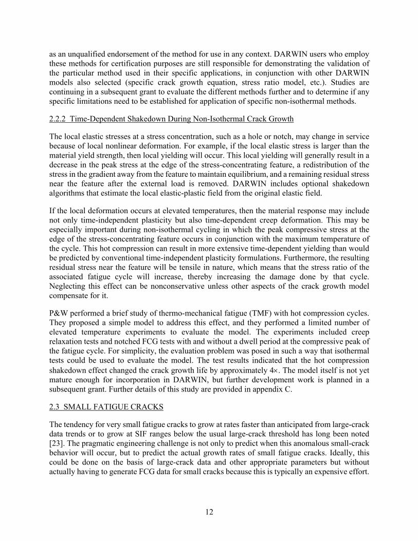
2.2.2 Time-Dependent Shakedown During Non-Isothermal Crack Growth

The local elastic stresses at a stress concentration, such as a hole or notch, may change in service because of local nonlinear deformation. For example, if the local elastic stress is larger than the material yield strength, then local yielding will occur. This local yielding will generally result in a decrease in the peak stress at the edge of the stress-concentrating feature, a redistribution of the stress in the gradient away from the feature to maintain equilibrium, and a remaining residual stress near the feature after the external load is removed. DARWIN includes optional shakedown algorithms that estimate the local elastic-plastic field from the original elastic field.

If the local deformation occurs at elevated temperatures, then the material response may include not only time-independent plasticity but also time-dependent creep deformation. This may be especially important during non-isothermal cycling in which the peak compressive stress at the edge of the stress-concentrating feature occurs in conjunction with the maximum temperature of the cycle. This hot compression can result in more extensive time-dependent yielding than would be predicted by conventional time-independent plasticity formulations. Furthermore, the resulting residual stress near the feature will be tensile in nature, which means that the stress ratio of the associated fatigue cycle will increase, thereby increasing the damage done by that cycle. Neglecting this effect can be nonconservative unless other aspects of the crack growth model compensate for it.

P&W performed a brief study of thermo-mechanical fatigue (TMF) with hot compression cycles. They proposed a simple model to address this effect, and they performed a limited number of elevated temperature experiments to evaluate the model. The experiments included creep relaxation tests and notched FCG tests with and without a dwell period at the compressive peak of the fatigue cycle. For simplicity, the evaluation problem was posed in such a way that isothermal tests could be used to evaluate the model. The test results indicated that the hot compression shakedown effect changed the crack growth life by approximately 4. The model itself is not yet mature enough for incorporation in DARWIN, but further development work is planned in a subsequent grant. Further details of this study are provided in appendix C.

2.3 SMALL FATIGUE CRACKS

The tendency for very small fatigue cracks to grow at rates faster than anticipated from large-crack data trends or to grow at SIF ranges below the usual large-crack threshold has long been noted [23]. The pragmatic engineering challenge is not only to predict when this anomalous small-crack behavior will occur, but to predict the actual growth rates of small fatigue cracks. Ideally, this could be done on the basis of large-crack data and other appropriate parameters but without actually having to generate FCG data for small cracks because this is typically an expensive effort.

13

A literature survey of small-crack effects in a variety of common gas turbine engine rotor materials was performed. The specific materials were Ti-6Al-4V; Ti-6Al-2Zr-4Sn-6Mo; IN-100; Udimet® 720; and Astroloy™. The database included a wide range of microstructures as well as multiple stress ratios and temperatures. Growth rate data for small fatigue cracks were critically compared against corresponding large-crack data. A simple engineering model for small-crack behavior first proposed by El Haddad [24] was critically evaluated by attempting to predict the small-crack growth rates from the large crack data for each material. Different methods of estimating the El Haddad length parameter a0, including the traditional calculation from large-crack threshold and endurance limit properties, as well as a new approach based on empirical scaling from microstructural dimensions, were explored and compared. Strengths and limitations of the simple El Haddad approach for engineering applications were considered, as well as the practical significance of small-crack effects for life prediction. Further description of this study is provided in appendix D.

The literature review revealed a surprising lack of small-crack data for the common nickel-based superalloy IN-718. Therefore, an experimental effort was initiated to generate growth-rate data for small fatigue cracks in this alloy. The activity was conducted at Honeywell using the same 718 alloy and general test procedures being employed in the benchmark FCG studies (see section 2.5 and appendix F for more details).

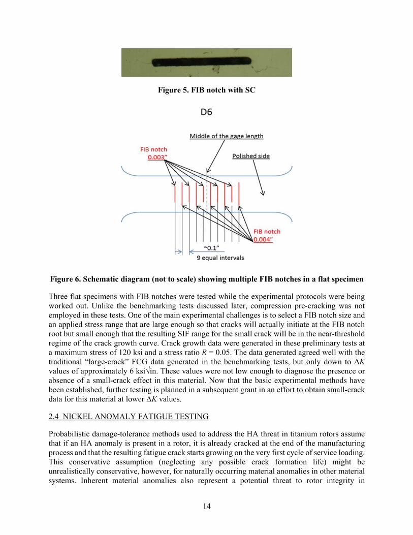
The basic specimen geometry was a flat tensile coupon. Focused ion beam (FIB) notches were machined on one polished face of each specimen so that very small fatigue cracks would form in predictable locations. These FIB notches were extremely small but had distinct and repeatable dimensions. FIB notches had a total surface length of either 0.002″, 0.003″, or 0.004″; a height of less than 0.001″; and a depth of approximately half of the surface length. An example FIB notch with a fatigue crack growing out of the notch is shown in figure 5. This particular notch had a total surface length of 0.003159″. Multiple FIB notches were placed on the same face of the same specimen to generate data for multiple cracks simultaneously. The notches were placed far enough away from each other to avoid crack interactions while the cracks remained in the small-crack size regime. Figure 6 is a schematic diagram (not to scale) showing the arrangement of multiple FIB notches on one of the developmental specimens. Note that the total width of the specimen gauge section was 0.6″.

14

Figure 5. FIB notch with SC

Figure 6. Schematic diagram (not to scale) showing multiple FIB notches in a flat specimen

Three flat specimens with FIB notches were tested while the experimental protocols were being worked out. Unlike the benchmarking tests discussed later, compression pre-cracking was not employed in these tests. One of the main experimental challenges is to select a FIB notch size and an applied stress range that are large enough so that cracks will actually initiate at the FIB notch root but small enough that the resulting SIF range for the small crack will be in the near-threshold regime of the crack growth curve. Crack growth data were generated in these preliminary tests at a maximum stress of 120 ksi and a stress ratio R = 0.05. The data generated agreed well with the traditional “large-crack” FCG data generated in the benchmarking tests, but only down to ΔK values of approximately 6 ksi√in. These values were not low enough to diagnose the presence or absence of a small-crack effect in this material. Now that the basic experimental methods have been established, further testing is planned in a subsequent grant in an effort to obtain small-crack data for this material at lower ΔK values.

2.4 NICKEL ANOMALY FATIGUE TESTING

Probabilistic damage-tolerance methods used to address the HA threat in titanium rotors assume that if an HA anomaly is present in a rotor, it is already cracked at the end of the manufacturing process and that the resulting fatigue crack starts growing on the very first cycle of service loading. This conservative assumption (neglecting any possible crack formation life) might be unrealistically conservative, however, for naturally occurring material anomalies in other material systems. Inherent material anomalies also represent a potential threat to rotor integrity in

15

conventional cast and wrought nickel-based superalloys (such as IN-718), although relatively few reported incidents have been associated with this type of anomaly. The FAA, in conjunction with RISC, may formally address this potential threat in the future. Therefore, it is important to better understand the possible significance of the crack-formation process for these types of anomalies.

Toward that end, P&W conducted a limited experimental investigation to characterize the impact of naturally occurring material anomalies on the fatigue performance of rotor grade conventional nickel material—specifically, double melted IN-718. This investigation involved the identification and procurement of material that appeared to contain significant material anomalies, forging and heat treatment of this material to rotor specification, additional NDE inspections, and the machining and testing of fatigue specimens for characterization. A summary of this investigation is provided in appendix E.

Initial procurement and inspection of billets containing potential anomalies and specimen fabrication from these billets was performed in a previous grant [8]. In the current grant, these billets were machined to create cylindrical fatigue specimens with the indicated material anomaly located in the interior of the gauge section. These specimens were then tested to failure under constant amplitude fatigue cycling. Three specimens were machined and two of these were tested successfully. These two tests were both conducted under load control at 60 CPM (1 Hz) and 1000F with R = 0.05 and a maximum stress of 130 ksi. During the fatigue testing, the specimens received potential drop monitoring, acoustic monitoring, and an HCF “buzz” to assist in understanding the contribution of crack nucleation relative to crack growth life. Post-test fractography was performed to characterize the initiating anomaly and the resulting FCG.

The two successful tests gave fatigue lifetimes of 114,976 cycles and 43,684 cycles, respectively. In both cases, attempts to detect early crack growth using direct current potential drop methods (with some assistance from post-test fractography) suggested that a significant fraction of the total fatigue life was associated with crack formation. The material anomaly cross-section size on the fracture plane was approximately 0.025″ × 0.007″ for the longer life specimen and 0.029″ × 0.052″ for the shorter life specimen.

2.5 BENCHMARK FCG DATA

Engineering SIF solutions are commonly verified analytically by comparison to more sophisticated numerical solutions. However, even the “exact” numerical solutions can exhibit some variability, depending on the quality of the method and the skill of the modeler. SIF solutions developed by different organizations for the same nominal geometry can exhibit noticeable differences. Furthermore, the ability of the mathematical SIF solutions alone to address geometrical effects, such as the interaction of the crack front with adjoining or approaching free surfaces, is remarkably unresolved in the literature. Experimental validation is needed to ensure that SIF solutions are formulated and implemented to give accurate predictions of FCG rate.

In this activity, a reliable database of FCG data on several different specimen geometries was generated for a carefully pedigreed rotor material to facilitate the evaluation of SIF solutions and related crack growth algorithms in the Flight_Life fracture mechanics module. All testing was performed at Honeywell on a fine-grained delta-processed Inconel 718 alloy (DP718) at 600F. Testing was performed on four different specimen geometries: a surface-crack tension (SC(T))

16

geometry at two different thicknesses, a corner-crack tension (CC(T)) geometry, and a center-hole geometry with a corner crack at the hole.

Analysis of the resulting data was performed at SwRI. The SC(T) test results were used to generate baseline FCG properties in the form of a Paris equation. This equation was used to back-predict the SC(T) test results to show consistency, and then the same equation was used to predict the completely independent tests on the other geometries. The results were also used to evaluate the question of whether constraint correction factors should be included in the DARWIN crack growth models for these geometries. The DARWIN SIF solution CC11 for a corner crack in a plate and the current DARWIN practice of including a constraint correction term at both tips of CC11 was shown to give an accurate prediction of the experimentally observed FCG rates. Evaluation of the DARWIN CC08 solution and the corresponding constraint correction for a corner crack at a hole was compromised by scatter in the available test results. Further details of the experiments, the data analysis, and the results are provided in appendix F.

Additional benchmark experiments were originally planned to be performed at SwRI with Ti-6Al-4V specimens testing at room temperature, but these tests could not be performed because of reductions in the grant budget. This work is planned for a subsequent grant.

3. ADVANCED FRACTURE ANALYSIS

Progress in advanced fracture analysis included the development and implementation of several new or enhanced SIF solutions, a new bivariant shakedown module, facilities permitting users to provide their SIF solutions in tabular form, an alternative stress ratio model, and a high-cycle fatigue threshold check.

3.1 NEW AND ENHANCED SIF SOLUTIONS

At the very heart of the damage-tolerance assessment is the calculation of the driving force for crack growth, the SIF, for a crack in a complex component with arbitrary stress gradients. This calculation must be performed both accurately and quickly to support practical reliability assessments. A number of original SIF solutions were generated for earlier versions of DARWIN, most supporting arbitrary stress gradients in one dimension (so-called univariant solutions), and a few supporting arbitrary stress gradients in all directions on the crack plane (so-called bivariant solutions). These were all WF formulations based on the stress distributions at the crack location in the corresponding uncracked body.

Several new WF SIF solutions were developed and implemented under the current grant to address a wider range of geometries and stress gradients commonly encountered in production rotors. In addition, several new integration and pre-integration methods were developed to improve the computational efficiency of the solutions. The details of these new developments are provided in appendix G. A short overview is provided in the following sub-sections.

3.1.1 New Bivariant SIF Solution for Semi-Elliptical SC in Plate

DARWIN previously included a univariant WF SIF solution for a semi-elliptical crack in a plate, denoted as SC17. However, this univariant solution cannot accommodate situations in which the stresses in the uncracked body change significantly along the surface because the only allowable stress

17

gradient extends into the depth (thickness) of the body. Therefore, a new bivariant solution, denoted SC19, was developed for the same crack and plate geometry. This solution was based on the same point weight function (PWF) and dynamic K interpolation methods employed in the corner crack solutions CC09 and CC10 [8,13] but uses slightly different boundary correction terms to account for SC features. Figure 7 shows the SC configuration, where the center of the SC is offset from the plate center by a distance B, and the stress variation is specified in two dimensions, in terms of either the global coordinate system (X,Y) or the local coordinate system (x, y).

The WF requires reference solutions for determining the coefficient defined inside the boundary correction terms. Some of the original reference solutions from the development of SC17 could be used for this purpose. Additional reference solutions were generated using the FADD3D boundary element software [25] for pre-defined cracked configurations subjected to unit tension or unit bending. FADD3D and the commercial FE software FEACrack™ were also used to generate independent solutions for verification of the WF solutions. Further details of the derivation and verification are provided in appendix G. The new SC19 solution was first implemented in DARWIN in Version 6.1.

Figure 7. Schematic for SC configuration of SC19

3.1.2 Extension of Validity Limits for Univariant SIF for Semi-Elliptical SC in Plate

The solution limits for SC17 (SC in plate subjected to univariant stressing along the thickness direction) were extended by taking advantage of the additional reference solutions generated when formulating SC19. In the new version, the offset of the crack can be located up to 90% from the plate center, the maximum crack depth and surface length are 90% of the plate thickness t and the surface ligament (bB), and the maximum crack aspect ratio is a/c = 8. The previous limits were 80% and a/c = 4. The SC17 geometry is the same as the SC19 geometry shown in figure 7.

 

y

2c

a

(X,Y) B

W=2b

t

X, x

Y

O

18

3.1.3 Improved Integration Methods for Bivariant SIF Solutions

The formulation for bivariant WF SIF solutions requires integrating the WFs over the crack surface. Even performing the integration directly using a numerical scheme, such as Gauss-Chebychev quadrature, is relatively time-consuming, especially with a convergence check, when compared with one-dimensional univariant solutions. Several steps have been implemented previously to reduce this computational burden, such as tabulating parts of the integration for interpolation and reducing the effective calls to the SIF modules by interpolating SIF results from dynamic SIF tables. In this effort, an additional algorithm was developed to further reduce the computation time substantially. This new algorithm approximates the customary double integration by a simple double summation based on tabular WF values and interpolated nodal stress. A brief description is provided in appendix G.

3.1.4 Pre-Integration Methods for Univariant SIF Solutions

Current DARWIN univariant SIF solutions for cracks with two or three degrees of freedom use the WFs originally proposed by Shen and Glinka [26]. The SIF solutions are determined by integrating the product of the WF and the stress component normal to the crack plane across the specified crack depth. The selected WF depends on the location of the crack tip (e.g., surface tip or deepest tip).

The integration is performed in one dimension whose direction is along the crack depth and currently is determined using the Gauss-Chebyshev numerical method with an iterative convergence check. However, the iterative process associated with the numerical integration for convergence can become time-consuming for steep stress gradients. Therefore, a new pre-integration method was developed to evaluate the SIF more efficiently.

The essence of this pre-integration scheme is to approximate the stress variation between user-specified stress values by Hermite polynomials and break down the entire integration into one single pass of simple summation such that no further iteration is necessary. The computation time therefore becomes consistent and does not depend on the stress gradient, whereas the results are almost identical with the current numerically integrated results (note that a linear variation between user-specified stress values is assumed in the current version). Further details are provided in appendix G.

3.1.5 New Univariant SIF Solution for Through Crack in Variable Thickness Plate

An approximate SIF solution was developed for a through-thickness edge crack in a variable-thickness plate depicted schematically in figure 8. The new crack configuration is denoted by TC15. The solution requires the thickness variation to be modeled as symmetrical to the mid-plane of the plate. TC15 is an approximate univariant WF solution based on the TC12 edge crack SIF solution and energy considerations. TC15 is the first SIF solution implemented in DARWIN that does not employ a rectangular plate geometry model.

The TC15 GUI allows the user to use the mouse to specify a piecewise linear thickness variation in the model, based on interrogation of the underlying FEM, and to visualize the resulting fracture model immediately. The linear segments can vary in number and length. The GUI is shown in figure 9. This solution was first implemented in DARWIN 7.0.

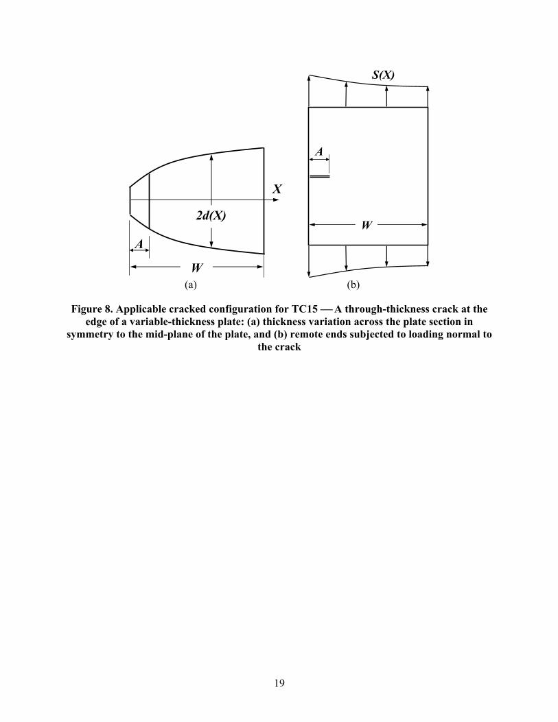
19

(a) (b)

Figure 8. Applicable cracked configuration for TC15 A through-thickness crack at the edge of a variable-thickness plate: (a) thickness variation across the plate section in

symmetry to the mid-plane of the plate, and (b) remote ends subjected to loading normal to the crack

X

2d(X)

A

W

A

W

S(X)

20

(a) (b)

(c) (d)

Figure 9. New GUI capability that enables the analyst to interactively create and edit fracture models for edge through cracks in plates of nonuniform thickness (TC15): (a)

FEM with non-uniform width features, (b) enlarged view of nonuniform width features, (c) TC15 fracture model superimposed on FE geometry in DARWIN GUI, and (d) TC15

fracture model coordinates and associated stress contour results

21

3.1.6 New Bivariant and Univariant SIF Solutions for Elliptical Embedded Crack in Plate

Two SIF solutions for an embedded crack in plate were developed and validated. The solutions are designated as EC04 for an embedded crack subjected to bivariant stressing and EC05 for the crack subjected to univariant stressing. The two solutions are based on the same crack configuration shown in figure 10 and makes use of the same reference solutions. The reference solutions were generated using the FADD3D computer program.

Figure 10. Notations used for the embedded crack configuration in a rectangular section

The methods used for evaluating the SIF are all WF based. The only differences are that (1) EC05 uses a smaller subset of the reference solutions used by EC04, and (2) EC05 makes use of a PWF derived for a 1D domain whereas EC04 uses a PWF for a 2D domain. EC05 was developed to reduce the execution time on the condition that the applied stress variation can be represented as unidirectional. In addition, both EC04 and EC05 solutions have their own polynomial versions when the applied stress can be approximated by a simple polynomial (EC05) or bi-polynomial (EC04) expression. Additional details about the formulation and validation of EC04 and EC05 are provided in appendix G. The new EC04 and EC05 solutions were first implemented in DARWIN 7.0.

Although EC05 duplicates the general capabilities of the previous EC02 univariant solution, the new EC05 solution was derived to preserve full quantitative consistency with the bivariant EC04 solution when the stress fields are truly univariant. EC04 and EC05 also provide a broader geometry range than EC02 because the embedded crack can approach very close to two adjacent free surfaces (EC02 could only approach very close to a single free surface). The old EC02 solution will remain available in DARWIN for some time to facilitate comparisons and the use of input decks from previous DARWIN versions. Limited studies to date have indicated that EC02 and EC05 provide similar results.

3.1.7 Enhanced Bivariant SIF Solution for Corner Crack in Plate With Non-Normal Corners

The SIF solution CC09 for a quarter-elliptical corner crack in a plate with a rectangular cross-section under general bivariant stressing normal to the crack plane has been available in DARWIN for many years. In 3D geometry mode, the solution is applied after a 3D model has been sliced along a principal stress plane to generate a 2D model. However, because of modeling round-

X

Y

x

y

Bt

Bw

b

T

W=2b

t=2T

a c

22

off errors, the resulting corner angle in the 2D slice model is sometimes not exactly perpendicular. In the past, this meant that the CC09 solution could not be applied because the bivariant WF integration schemes were based on a perpendicular corner angle. Therefore, it was desirable to enhance the CC09 solution to permit it to be applied to corner angles that deviated slightly from 90. In this enhanced version, the maximum permissible angular variation of the corner from 90 is 5. Further details about the development of this new feature are provided in appendix G. The corresponding GUI capability is shown in figure 11. This enhanced solution was first implemented in DARWIN 7.1.

(a) (b)

Figure 11. New GUI capability for bivariant corner cracks (CC09) at non-normal corners: (a) placement of CC09 at a non-normal corner in the FEM, and (b) adjustment of CC09

corner angle to match the FE geometry

3.1.8 Integration of New Univariant SIF Solution for Corner Crack in Plate

A new univariant WF SIF solution for a corner crack in a plate, denoted CC11, was implemented in DARWIN. This solution was developed by SwRI under independent NASA funding and made available to DARWIN at no cost. The new crack model was based on FADD3D reference solutions generated previously under FAA funding to support the bivariant WF solution for a corner crack in plate, CC09. The new solution CC11 gives the same result as CC09 for a univariant stress gradient. However, the CC11 computation is faster because the WF formulation is limited to univariant gradients. The efficiency of the new solution was further increased by employing the pre-integration method described in appendix G. The new SC19 solution was first implemented in DARWIN in Version 6.1.

3.1.9 Revisions to Available Crack Model Solutions in DARWIN

Crack model SC02 was renamed SC17 to correspond to the same designation in NASGRO®. Crack model TC12 was renamed TC13 to correspond to the same designation in NASGRO. These changes were first implemented in DARWIN 6.1.

23

The crack-at-hole models formerly designated as SC15, CC05, and TC11 were removed from DARWIN 6.1 and later versions. These models were obsolete solutions that had been previously superseded by SC18, CC08, and TC13 but had been left in place temporarily for continuity.

Corner-crack-in-plate solutions were not previously available in surface damage (1D or 3D) mode. The CC09 bivariant solution and the new CC11 univariant solution were added to the appropriate surface-damage analysis modes beginning in DARWIN 6.1.

Crack-at-hole models SC18, CC08, CC10, and TC13 were not previously available in inherent (2D) mode. This availability was added in DARWIN 6.1 as part of the Kt functionality.

3.2 BIVARIANT SHAKEDOWN MODULE

DARWIN damage-tolerance analysis is customarily based on elastic finite element analysis (FEA) of stresses in the component. However, in some cases, the local elastic stress at a stress concentration feature may exceed the material yield strength. This implies that some local yielding would occur, causing a corresponding reduction and redistribution of the local elastic stress following the yielding event and the formation of a residual stress when the applied loading was removed. This phenomenon is sometimes called “shakedown” to denote that the local yielding occurs the first time that the maximum load is experienced but results in a stable elastic state for the remainder of the load history. Shakedown models provide an approximate calculation of the actual elastic-plastic stress distribution so that a full elastic-plastic FEA is not required. DARWIN has contained a shakedown module for many years that addresses univariant stress gradients. However, this univariant shakedown module was not sufficient to address the multi-dimensional stress gradients associated with bivariant WF solutions.

A new shakedown module for bivariant stressing was developed following a methodology detailed previously [27] but without the more complex material-hardening model. This methodology is for proportional loading and is applicable to 2D rectangular load-bearing sections whose elastic stress results are available and provided by the user as input. It predicts the elastic-plastic stress state after one-time shakedown. The analysis requires all six components of stress across the load-bearing section to determine the elastic-plastic stress state after shakedown, wherein the normal component to the net section is used for load shedding and convergence checks. The user-provided elastic stress variation has to be specified at the coordinate locations where the rectangular grid is defined. The methodology converts the linear elastic solution into an elastic-plastic solution while conserving forces and moments. The new bivariant shakedown module was first implemented in DARWIN 7.0.

Because the relative ratio between the plastic zone and the whole load-bearing section affects the load-shedding process resulting from converting elastic stresses to elastic-plastic stresses and, subsequently, the numerical convergence through iterations, the software module interpolates a set of intermediate stress values based on a more refined mesh of rectangular grid before beginning the shakedown analysis.

24

The bivariant shakedown methodology implemented in DARWIN can be resolved into the following steps:

Step (1): Generation of bivariant stress values at locations of grid points corresponding to a much more refined mesh of rectangular elements than the original mesh that designates the linear elastic solution.

Step (2): Evaluation of the resulting force normal to the load bearing section and the bending moments with respect to the x- and y-axes, based on the interpolated elastic stress variation defined at the refined mesh.

Step (3): Estimation of the plastic zone size, based on the von Mises stress criterion using the interpolated elastic stress variation.

Step (4): Stratification of the elastic stress variation according to the equivalent stress formulation into stress bands such that the area associated with each stress band can be identified and determined. The stress bands play an important role during load shedding process.

Step (5): Evaluation of the load shedding areas associated with the stress bands. It should be noticed that the stress bands are derived from the stratified stress variation that varies iteration by iteration, and thus the area distribution for load shedding changes.

Step (6): Determination of the plastically relaxed stresses for each equivalent stress band by applying Neuber’s rule, where the product of stress and strain is invariant with respect to the provided elastic and elastic-plastic material constitutive relationships between stress and strain. This approximation determines the relaxed equivalent elastic-plastic stress and strain.

Step (7): Determination of the elastic-plastic stress components from the relaxed equivalent elastic-plastic stress through iterations using the elastic stress component as the initial guess.

Step (8): Redistribution or load shedding of the excess incremental load arising from plastic stress relaxation over the area associated with each equivalent stress band. This is designated as local load shedding. To complete all local load shedding, steps 5–8 need to be repeated for each stress band.

Step (9): Calculation and redistribution of the global incremental loads needed to maintain force and moment balance after the plastic stress-relaxation process is completed on the load-bearing section. If convergence is achieved (i.e., force and moment balance are maintained), the iteration stops. Otherwise, steps 3–9 are repeated until global balance is achieved.

Step (10): Evaluation of the shakedown stress derived from the difference between the predicted elastic-plastic stress and the user-provided elastic stress at the locations of grid points designating the refined mesh. The shakedown stress corresponding to the original mesh is then interpolated.

Select comparisons between the elastic-plastic stress variations from FEA and from the bivariant shakedown module are shown in figures 12 and 13. The geometric configuration and load condition are for a notched plate of root radius r subjected to remote tension. The nonlinear elastic-plastic constitutive relationship was governed by the Ramberg-Osgood power law = 0/E[/0

25

+ (/0)]. Two material behaviors were considered: one, denoted by MATL-A, behaves more like an elastic-perfectly-plastic material; the other, denoted by MATL-B, demonstrates large capacity for strain hardening. Figure 12 shows the comparison for MATL-A, in which figures 12(a) and 12(b) plot the stress variations extracted directly from elastic and elastic-plastic FEAs, respectively, and figure 12(c) shows the predicted elastic-plastic stress variation from the shakedown module. The plotted stress component is normal to the load-bearing section originating from the root of the notch. The y-direction is along the bore of the hole, and the x-direction is from the root of the notch along the plate width direction. A similar comparison is shown in figure 13 for MATL-B. As indicated in these comparisons, not only does the shakedown methodology developed in DARWIN capture the salient features of elastic-plastic stress variation due to shakedown, but it also provides an excellent estimate on the quantitative stress values within a few percent.

(a) (b) (c)

Figure 12. Comparison of predicted elastic-plastic stress results from bivariant shakedown module with FEA results for MATL-A: (a) stress variation from elastic FEA, (b) stress

variation from elastic-plastic FEA, and (c) predicted elastic-plastic stress variation from shakedown module

26

(a) (b) (c)

Figure 13. Comparison of predicted elastic-plastic stress results from bivariant shakedown module with FEA results for MATL-B: (a) stress variation from elastic FEA, (b) stress

variation from elastic-plastic FEA, and (c) predicted elastic-plastic stress variation from shakedown module

3.3 FACILITIES FOR USER-SUPPLIED SIF TABLES

The library of SIF solutions in DARWIN are all based on idealized geometrical representations of the crack and cracked body. Cracked bodies are generally rectangular prisms, whereas cracks are planar and have perimeters that are either straight or part-elliptical. These idealizations are required to enable the SIF solutions to be derived/calculated in advance, so that the actual determination of the SIF values during a DARWIN run can be done very quickly. Experience has shown that these idealizations are entirely adequate in many practical rotor analyses, because many fatigue cracks do remain approximately flat and take on approximately straight or elliptical shapes, and irregular component boundaries are often far away from the crack. However, in some unique situations, actual fatigue cracks do not observe these conventions: the plane of crack growth can kink or curve, and the crack boundary can take on irregular shapes. In other cases, the explicit assumption that crack growth does not cause a significant redistribution of the applied loads is violated.

For these unique situations, it is still possible to calculate the SIF (and the crack shape evolution) using rigorous 3D numerical methods, such as boundary element methods or FEMs. In fact, such software as FADD-3D or FEACrack, which have been employed by the project team to derive library solutions can be used to calculate feature-specific solutions. However, there was previously no way to import these specific numerical solutions into DARWIN.

A new capability has now been implemented in DARWIN, beginning with Version 7.1, that allows the user to import a table of SIF values into DARWIN for use in life and fracture risk computations. The crack size is characterized by a single-length parameter with a definition established by the user. The user is responsible for determining the appropriate shape of the crack, including any crack geometry transitions, when generating the SIF solution table. Cracks with multiple dimensions (e.g., length and depth) are assumed to grow with an evolving shape that is the same in the analysis used to generate the input table as in the resulting DARWIN analysis. To use this feature, the user specifies the crack type as KA01 (user-defined K table, where K is a shorthand notation for the SIF) in the GUI zone editor (figure 14), and provides a text file that includes tables consisting of SIFs as a function of crack-size (SIF vs. a) values for the zones that use this crack

27

type. During execution, DARWIN reads the data directly from the file as needed, and uses the SIF values to calculate crack growth rates (the tabulated crack-size values are not used in the growth rate analysis). Additional optional columns in the defined table format can include the characteristic temperature, inspection variables such as the inspection “size” (area or length) corresponding to each index crack size, and stresses at the crack-tip location in the corresponding uncracked body. This capability is initially limited to a single mission and will be enhanced in the future to support multiple missions and SIF values arising from residual stresses.

Figure 14. GUI window for zone editor showing new capability for user-supplied K tables

3.4 ALTERNATIVE STRESS RATIO MODEL BASED ON STRESS LEVEL SENSITIVITY

P&W has developed an alternative stress ratio model for fatigue cycles containing nominally negative (compressive) stresses. This model and its supporting theory were documented in appendix B. The alternative model is particularly needed to use SIF values generated by FE simulations of growing cracks because the conventional definition of stress ratio in terms of Kmin/Kmax is not meaningful when a compressive stress is applied to the model and the crack itself is closed (i.e., Kmin is not defined). This so-called stress level sensitivity (SLS) model was implemented in DARWIN 7.1 as an additional option for a single crack-growth model, the NASGRO equation. This is achieved by modifications to several of the NASGRO equation parameters (e.g., crack closure function f, threshold SIF range) within DARWIN. Following additional study and evaluation of this new model, it may be extended to other DARWIN crack-growth models.

28

3.5 HCF THRESHOLD CHECK

A new capability was implemented in DARWIN 7.1 that allows the user to include the influence of vibratory high-cycle fatigue (HCF) stress values in FCG and fracture risk computations. Fracture is conservatively assumed to occur when the SIF range associated with the HCF stress alone exceeds the HCF FCG threshold property value provided by the user; no calculation of FCG due to HCF stresses is performed. The HCF threshold check is performed once per mission in conjunction with the application of the peak low-cycle fatigue (LCF) stress in the mission, at an average stress defined by that peak LCF stress. The user provides either the range or the amplitude of the HCF stress (figure 15). HCF stresses are not included in the calculation of crack-growth rates associated with LCF cycles.

Figure 15. GUI screens for new HCF threshold check capability in DARWIN

4. ADVANCED PROBABILISTIC METHODS

A new capability was also developed to predict the number of flight cycles associated with a user-specified probability of fracture. A conceptual model was also developed to efficiently generate approximate risk contours that can be used to guide the autozoning process.

4.1 COMPUTING LIFE FOR A SPECIFIED PROBABILITY OF FRACTURE

In previous versions of DARWIN, the probability of fracture was reported for a user-specified number of flight cycles. If users needed to know the number of flight cycles associated with the target risk, they had to adjust the input by trial and error until the desired result was obtained. A capability was developed that predicts the number of flight cycles associated with a user-specified

29

probability of fracture (target risk) value. To use this feature, the user specifies use of a target Pf value and enters the target value in the GUI, as shown in figure 16.

Figure 16. User specification of a target Pf value in the DARWIN GUI to activate the “life for a specified probability of fracture” capability

An algorithm was developed that efficiently estimates the number of flight cycles based on a user-specified probability-of-fracture value. The algorithm estimates an upper-bound target service life using the existing DARWIN Life Approximation Function (LAF) method with a relatively coarse mesh of initial anomaly sizes. This approach is very efficient (it requires only 20 life calculations per zone) but less accurate than the other probabilistic methods in DARWIN (e.g., Monte Carlo simulation, importance sampling). However, because the method is used only to estimate an upper-bound value (a complete DARWIN analysis is performed after the upper-bound target life is identified), the reduced accuracy is more than sufficient for this purpose. Moreover, the algorithm provides treatment for additional factors, including stress concentrations and manufacturing credits.

Figure 17 shows the general format of the results associated with this capability. The red horizontal line indicates the user-specified probability of fracture value, and life values are displayed at the locations where the risk curves intersect this line.

30

Figure 17. DARWIN “life for a specified probability of fracture” capability; life values are displayed at the locations where risk curves intersect the user-specified probability of

fracture value (indicated in the figure as a red horizontal line)

4.2 APPROXIMATE RISK CONTOURS

A conceptual model was developed to efficiently generate approximate risk contours based on the life contours capability in DARWIN. For this model, a family of risk contour values is created for key anomaly sizes associated with the anomaly distribution for a given material. Once the life contours have been identified, the probability density values associated with the individual anomaly sizes are transformed into probability density values associated with crack growth life, as shown in figure 18. The resulting crack-growth life probability density function can be used to compute the probability of fracture associated with a specified service life. Note that this approach considers only the influence of anomaly size, which is the dominant random variable for many materials. This conceptual model will be considered for future application to autozoning, in which the approximate risk contours will be used to guide the dimensions of the initial zone mesh.

31

Figure 18. Conceptual model for predicting approximate risk contour values in which an anomaly distribution is transformed into a crack-growth life distribution via life contours

associated with key anomaly sizes

5. ADVANCED ZONING CAPABILITIES

The overall objective of this task was to provide new capabilities to automate the zone-creation process. Additional objectives were to enable application of stress concentration factors to FE stress results and to provide new capabilities for zoning of selected surfaces of a component.

A DARWIN capability to address stress concentration factor (Kt) gradients in 2D axisymmetric models was developed to support titanium HA anomaly distribution recalibration efforts within RISC. The capability was extended to provide treatment for stress concentrations that are in the vicinity of turned surfaces.

A new surface zoning capability for 2D axisymmetric FE models was implemented in DARWIN to provide support for risk assessment of turned surfaces. A DARWIN capability for surface-damage assessment of blade slots was also developed to support ongoing RISC activities.

Automated modeling capabilities were implemented in DARWIN to reduce the variability in the current analysis process that can be introduced by the human operator. These capabilities consist of automatic construction of fracture mechanics models (autoplate), life contours, and autozoning. The autoplate algorithm automatically determines the initial crack type and the orientation and size of an idealized fracture mechanics plate model associated with 2D FEM geometry and stress results. Autoplate is used to construct life contours based on initial cracks placed at each of the nodes in an FEM. Risk contours are developed in a similar fashion to life contours, except that a distribution of initial crack sizes is applied at each FE. The process of automated risk contour creation is also referred to as autozoning.

ac

a

NTarget N

P(a

)

P(N)

Pf

ac

a

NTarget N

P(a

)

P(N)

Pf

32

These capabilities are described in more detail in the following sections.

5.1 TREATMENT OF STRESS CONCENTRATIONS IN 2D MODELS

A DARWIN capability to address stress concentration factor (Kt) gradients in 2D axisymmetric models was developed to support titanium HA anomaly distribution recalibration efforts within RISC. As shown in figure 19, the capability is used to model the stress values at cross-sections with and without holes (cross-sections I and II, respectively). The analyst provides a 2D axisymmetric FEM with hole elements removed. A GUI menu is provided that allows the analyst to describe the extent of the region over which the Kt gradient is applied. The analyst also provides values of Kt versus physical distance from the starting edge of the Kt region, which defines the length of the Kt region. Stress values within a Kt region are based on the product of Kt values and FE stress results within the region.

(a) (b) (c)

Figure 19. Disk cross sections influenced by stress concentration (Kt) effects: (a) axial view of disk indicating location of slices, (b) cross-section through hole and associated Kt region,

and (c) cross-section without holes (without Kt)

To use this feature, the analyst specifies use of “stress concentration profiles” in the GUI setup menu (figure 20). When the feature is enabled, DARWIN will automatically identify zones that have stress gradients that fall within a Kt region, allowing the user to specify properties with and without the influence of Kt. Note that hole elements are not included in the analyst-provided FEM, so the holes are “virtually filled” for risk computations associated with the cross-section without holes. Stress values at locations within the virtually filled holes are approximated from an interpolation of stress values at nodes along the edges of the hole. For example, the stress at point C shown in figure 21 is based on a linear interpolation of values at points A and B. The stress values at points A and B are based on interpolation of the nearest FE nodes.

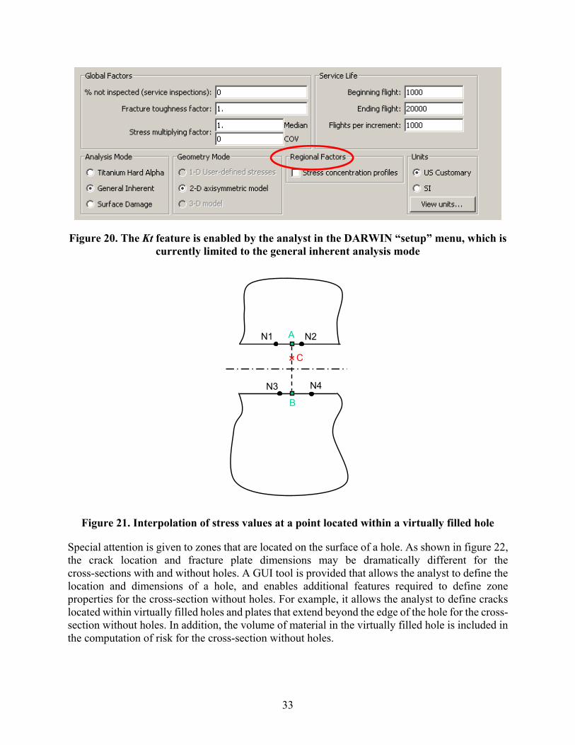
33

Figure 20. The Kt feature is enabled by the analyst in the DARWIN “setup” menu, which is currently limited to the general inherent analysis mode

Figure 21. Interpolation of stress values at a point located within a virtually filled hole

Special attention is given to zones that are located on the surface of a hole. As shown in figure 22, the crack location and fracture plate dimensions may be dramatically different for the cross-sections with and without holes. A GUI tool is provided that allows the analyst to define the location and dimensions of a hole, and enables additional features required to define zone properties for the cross-section without holes. For example, it allows the analyst to define cracks located within virtually filled holes and plates that extend beyond the edge of the hole for the cross-section without holes. In addition, the volume of material in the virtually filled hole is included in the computation of risk for the cross-section without holes.

N1 N2

N3 N4

A

B

C

N1 N2

N3 N4

A

B

C

34

Figure 22. “Kt-affected” zone at the surface of a hole: (a) cross-section through hole including effect of Kt (with Kt) and (b) cross-section without holes (without Kt) (Note that

the zone volume, crack location, and plate dimensions may differ for the two cross-sections)

Risk results are provided for the cross-section with holes (with Kt) and the cross-section without holes (without Kt). Also provided is the combined risk of the two cross sections, defined as:

(7)

where is the zone risk, and are the risks associated with cross sections

with and without holes, respectively, and is the Kt contribution factor.

The growth rates of cracks originating on turned surfaces may also be influenced by stress concentrations near hole features. A capability was implemented for assessment of turned surfaces near stress concentrations. It was based on existing DARWIN features for treatment of turned surfaces (2D Surface Damage Analysis mode) and stress concentration (Kt) effects (General Inherent Analysis mode). As shown in figure 23, the new capability enables the user to define Kt regions near stress concentrations, such as holes. The Kt gradient associated with the Kt region is automatically applied to crack-growth computations for zones with stress gradients that fall within the Kt region.

With Kt Without Kt

Kt region Plate

ZoneAnomaly

AnomalyPlate

Zone

, ,1f Kt f with Kt Kt f without KtP P P

fP ,f with KtP ,f without KtP

Kt

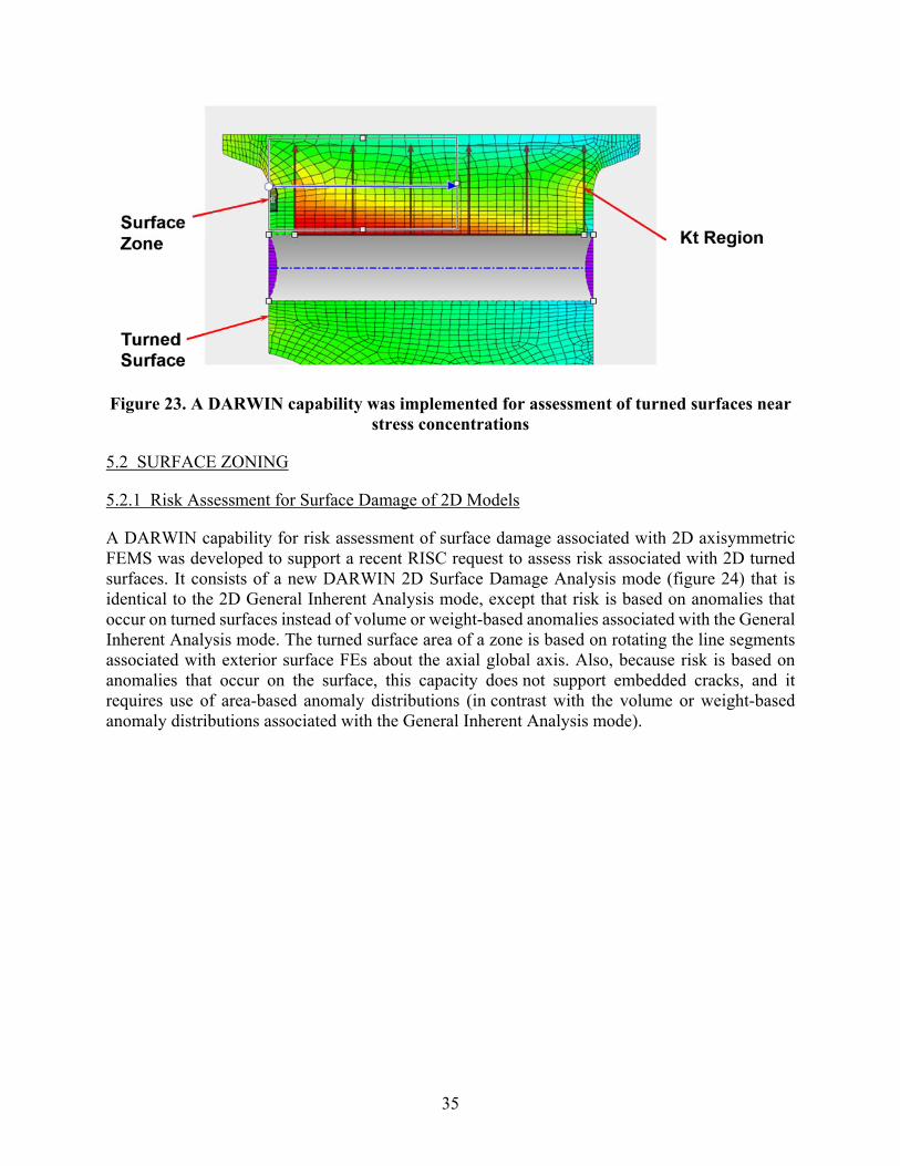
35

Figure 23. A DARWIN capability was implemented for assessment of turned surfaces near stress concentrations

5.2 SURFACE ZONING

5.2.1 Risk Assessment for Surface Damage of 2D Models

A DARWIN capability for risk assessment of surface damage associated with 2D axisymmetric FEMS was developed to support a recent RISC request to assess risk associated with 2D turned surfaces. It consists of a new DARWIN 2D Surface Damage Analysis mode (figure 24) that is identical to the 2D General Inherent Analysis mode, except that risk is based on anomalies that occur on turned surfaces instead of volume or weight-based anomalies associated with the General Inherent Analysis mode. The turned surface area of a zone is based on rotating the line segments associated with exterior surface FEs about the axial global axis. Also, because risk is based on anomalies that occur on the surface, this capacity does not support embedded cracks, and it requires use of area-based anomaly distributions (in contrast with the volume or weight-based anomaly distributions associated with the General Inherent Analysis mode).

36

Figure 24. New DARWIN 2D surface-damage analysis mode that was developed to assess risk associated with 2D turned surfaces

5.2.2 Surface Area of Blade Slots

A DARWIN capability for surface damage assessment of blade slots was developed to support ongoing RISC activities. The risk of fracture at blade slots is dependent on (1) the probability that a crack occurs on the slot surface; and (2) the probability of fracture given that a crack occurs on the slot surface. The probability that a crack occurs on the blade slot surface is based on the anomaly distribution for blade slots per unit area and the surface area of each blade slot. An anomaly distribution for blade slots will be developed by RISC. A new DARWIN capability was needed to identify the area of the blade slots.

As shown in figure 25, a new capability was implemented in DARWIN to assist the user in the quantification of the surface area of blade slots in 3D FEMs. It includes GUI controls that allow the user to specify the FE faces to include in the assessment (figure 26). The capability has been successfully tested on several blade slot attachment models that were provided by GE and P&W.

37

(a)

(b)

Figure 25. A new capability to quantify the surface area of blade slots in 3D FEMs was implemented in DARWIN; user selection of (a) a single surface region and (b) multiple

surface regions

38

Figure 26. The new blade slot area quantification capability includes controls to specify the FE faces that are included in the assessment

5.3 AUTO-MODELING

One of the major efforts for the referenced grant was the development of automated modeling capabilities to assist the user in building fracture mechanics and zone models. These capabilities reduce the variability in the current analysis process that can be introduced by the human operator. The automated modeling consists of automatic construction of fracture mechanics models (autoplate), life contours, and autozoning. The autoplate algorithm automatically determines (without requiring user intervention) the initial crack type and the orientation and size of an idealized fracture mechanics plate model that will give accurate FCG life results, given only a 2D FEM with stress results and the initial location of a crack in the model. To construct a life contour, an initial crack size is placed at each of the nodes in an FEM, autoplate is applied to define the fracture mechanics model at each node, the FCG life is computed at each node, and then a life contour plot is created based on the life values at the nodes. Risk contours are developed in a similar fashion to life contours, except that a distribution of initial crack sizes is applied at each element centroid, and risk values are computed based on the distribution of crack sizes and other random variables as well. The process of automated risk contour creation is also referred to as autozoning.

5.3.1 Automatic Construction of Fracture Models

The unique GUI functionality of DARWIN permits the analyst to quickly construct fracture models from the FEM, using the mouse to fix the location, size, and orientation of a simplified

39

rectangular plate model that is superimposed on the FE slice. However, the quality of the resulting fracture model still depends on the skill and judgment of the analyst, which can be problematic if he or she has limited experience or formal training in fracture mechanics. Furthermore, integrity analysis of components in which fatigue cracks can form at material anomalies located anywhere in the volume of the component (as is the case for titanium HA, for example) may require the construction of large numbers of fracture models. Even with the GUI tools, this can still be a time-consuming and expensive process.

An alternative scheme has been developed for DARWIN that automatically determines (without user input) the orientation, size and stress input for a fracture model that will produce accurate life results, given only the 2D model (or slice) and the initial crack location. The new automatic fracture model generation module (included in DARWIN version 7.0) emulates the judgment of an experienced user by orienting and sizing a rectangular plate fracture model to reflect the actual component boundaries in the vicinity of a surface, corner, or embedded crack. The specific algorithms developed to perform these functions are briefly described in the following paragraphs, accompanied by illustrations from DARWIN.

A first-generation automatic fracture model algorithm based on rectangular plate models was previously developed by Emery et al. [28] as part of a larger effort to develop a multi-scale damage and durability simulation methodology. However, that approach was limited to simplified stress gradients and to semi-infinite geometry models that neglected most boundary effects. Although it performed well for a limited set of simple test coupon geometries used in demonstration problems, it would not be able to address the complex component shapes of mechanical components, such as gas turbine engine rotors.

5.3.1.1 Selecting Plate Orientation

One major challenge to selecting the plate orientation is that the angles of the major and minor plate axes are relative to the component geometry. For cracks on the component surface, this is usually straightforward: one edge of the plate will be tangent to the component boundary at the initial crack location. The crack will then grow away from this edge, and the other boundaries may or may not become significant as the crack grows. This orientation is shown in figure 27 for an axisymmetric impeller model.

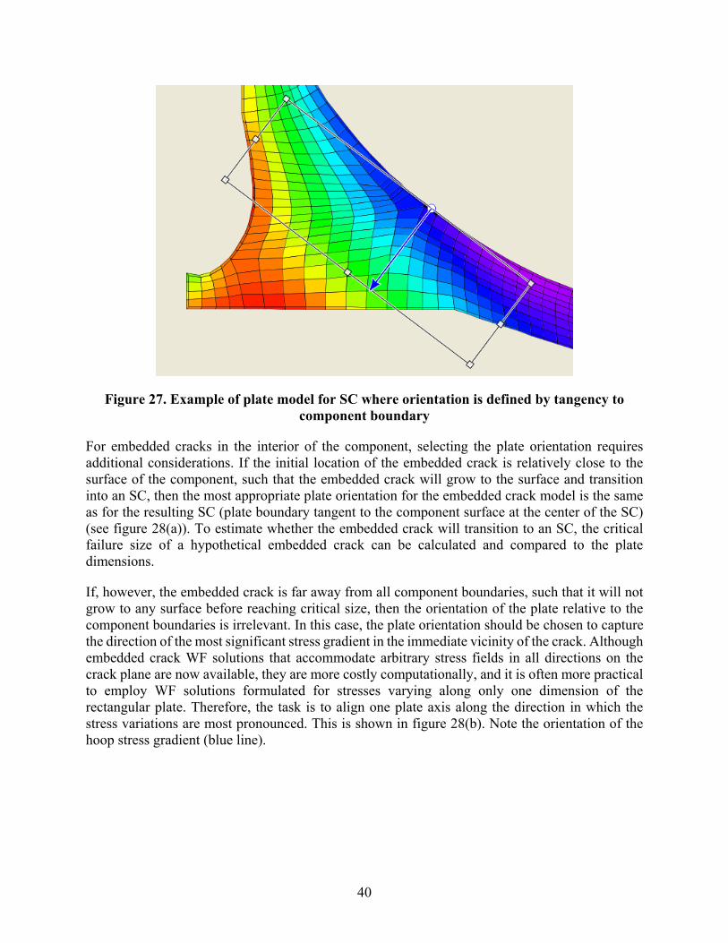
40

Figure 27. Example of plate model for SC where orientation is defined by tangency to component boundary

For embedded cracks in the interior of the component, selecting the plate orientation requires additional considerations. If the initial location of the embedded crack is relatively close to the surface of the component, such that the embedded crack will grow to the surface and transition into an SC, then the most appropriate plate orientation for the embedded crack model is the same as for the resulting SC (plate boundary tangent to the component surface at the center of the SC) (see figure 28(a)). To estimate whether the embedded crack will transition to an SC, the critical failure size of a hypothetical embedded crack can be calculated and compared to the plate dimensions.

If, however, the embedded crack is far away from all component boundaries, such that it will not grow to any surface before reaching critical size, then the orientation of the plate relative to the component boundaries is irrelevant. In this case, the plate orientation should be chosen to capture the direction of the most significant stress gradient in the immediate vicinity of the crack. Although embedded crack WF solutions that accommodate arbitrary stress fields in all directions on the crack plane are now available, they are more costly computationally, and it is often more practical to employ WF solutions formulated for stresses varying along only one dimension of the rectangular plate. Therefore, the task is to align one plate axis along the direction in which the stress variations are most pronounced. This is shown in figure 28(b). Note the orientation of the hoop stress gradient (blue line).

41

(a)

(b)

Figure 28. (a) Example of plate model for embedded crack where orientation is defined by nearby component boundary; (b) example of plate model for embedded crack where

orientation is defined by significant stress gradient

42

5.3.1.2 Selecting Plate Size

Another major challenge is selecting the appropriate size (height and width) of the rectangular plate model. If the component boundaries are far away from the crack, then this is simple; an infinite plate model is adequate. However, if the growing crack approaches component boundaries in any direction, then the finite plate size in that direction is defined so that the effect of the free surface is adequately captured.

One of the algorithms used to fix plate sizes is shown in figure 29. In this example, an embedded crack is located at the origin of the coordinate system, and the coordinate system orientation has been defined by the point of tangency on the component boundary nearest to the crack (because the growing embedded crack will transition to an SC). Trial plate boundaries (blue dashed lines) are defined by the intersection of the plate axes with the component boundaries. Each quadrant is bisected by a diagonal from the crack origin, and updated plate boundaries (dashed red lines) are defined by the minimum distance from the crack origin to the component boundary in each half of each quadrant. These updated boundaries may be further modified by similar constructions in the other quadrants, ensuring that the final plate boundaries represent the minimum size indicated by any quadrant.

Figure 29. Plate-sizing algorithm

The final plate may not necessarily be contained entirely within the component boundaries, but there is generally an adequate net section area elsewhere in the component (outside the plate model) to accommodate this load. The essential constraint is that the crack itself should not grow beyond the component boundaries, and the plate algorithm shown in figure 29 is intended to enforce this constraint for elliptical cracks. Also, most of the FCG life will usually be consumed

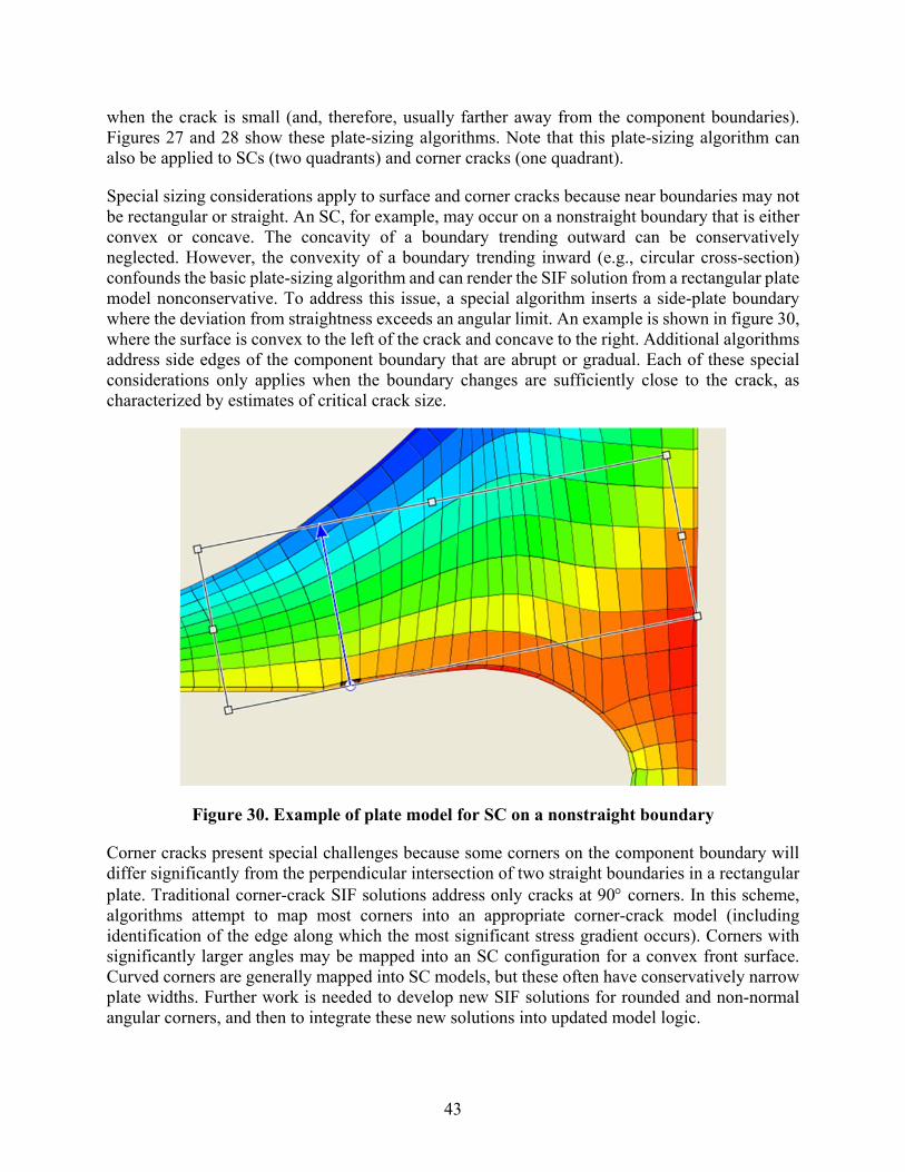
43

when the crack is small (and, therefore, usually farther away from the component boundaries). Figures 27 and 28 show these plate-sizing algorithms. Note that this plate-sizing algorithm can also be applied to SCs (two quadrants) and corner cracks (one quadrant).

Special sizing considerations apply to surface and corner cracks because near boundaries may not be rectangular or straight. An SC, for example, may occur on a nonstraight boundary that is either convex or concave. The concavity of a boundary trending outward can be conservatively neglected. However, the convexity of a boundary trending inward (e.g., circular cross-section) confounds the basic plate-sizing algorithm and can render the SIF solution from a rectangular plate model nonconservative. To address this issue, a special algorithm inserts a side-plate boundary where the deviation from straightness exceeds an angular limit. An example is shown in figure 30, where the surface is convex to the left of the crack and concave to the right. Additional algorithms address side edges of the component boundary that are abrupt or gradual. Each of these special considerations only applies when the boundary changes are sufficiently close to the crack, as characterized by estimates of critical crack size.

Figure 30. Example of plate model for SC on a nonstraight boundary

Corner cracks present special challenges because some corners on the component boundary will differ significantly from the perpendicular intersection of two straight boundaries in a rectangular plate. Traditional corner-crack SIF solutions address only cracks at 90 corners. In this scheme, algorithms attempt to map most corners into an appropriate corner-crack model (including identification of the edge along which the most significant stress gradient occurs). Corners with significantly larger angles may be mapped into an SC configuration for a convex front surface. Curved corners are generally mapped into SC models, but these often have conservatively narrow plate widths. Further work is needed to develop new SIF solutions for rounded and non-normal angular corners, and then to integrate these new solutions into updated model logic.

44

5.3.2 Life Contours

The automatic fracture geometry model capabilities have been employed to generate life contour maps for complex components. A fatigue crack of user-specified constant initial size or area is placed virtually at every node in the FE model. The automatic geometry model process is invoked to generate a fracture model for each crack, and then the FCG lifetime to failure (or runout) is calculated for each model. This life calculation can employ FE stress results at multiple time steps, using rainflow cycle counting to pair individual time steps into appropriate stress cycles. For efficiency reasons, this calculation currently uses only univariant SIF solutions, but this is a limitation that can be removed in future implementations, albeit with some loss of efficiency.

The resulting family of calculated life results can be visualized in the GUI using conventional contouring methods, as is often done for stresses. Example results are shown in figures 31 and 32. The images on the left show the stress contours, and the images on the right show the corresponding FCG life contours. The life contours are shown as the logarithm (base 10) of the calculated life because fatigue lives span a wide range and vary nonlinearly. These figures demonstrate that the stress hot spots (red regions of especially high stress) do not correspond exactly with the life hot spots (regions of especially low FCG life) because of the additional geometry factors that influence FCG life. This capability was first included in DARWIN version 7.1.

(a) (b)

Figure 31. (a) Hoop stress contour plot for part of an axisymmetric ring disk geometry; (b) corresponding life contour plot

45

(a)

(b)

Figure 32. (a) Hoop stress contour plot for part of an axisymmetric impeller geometry; (b) corresponding life contour plot

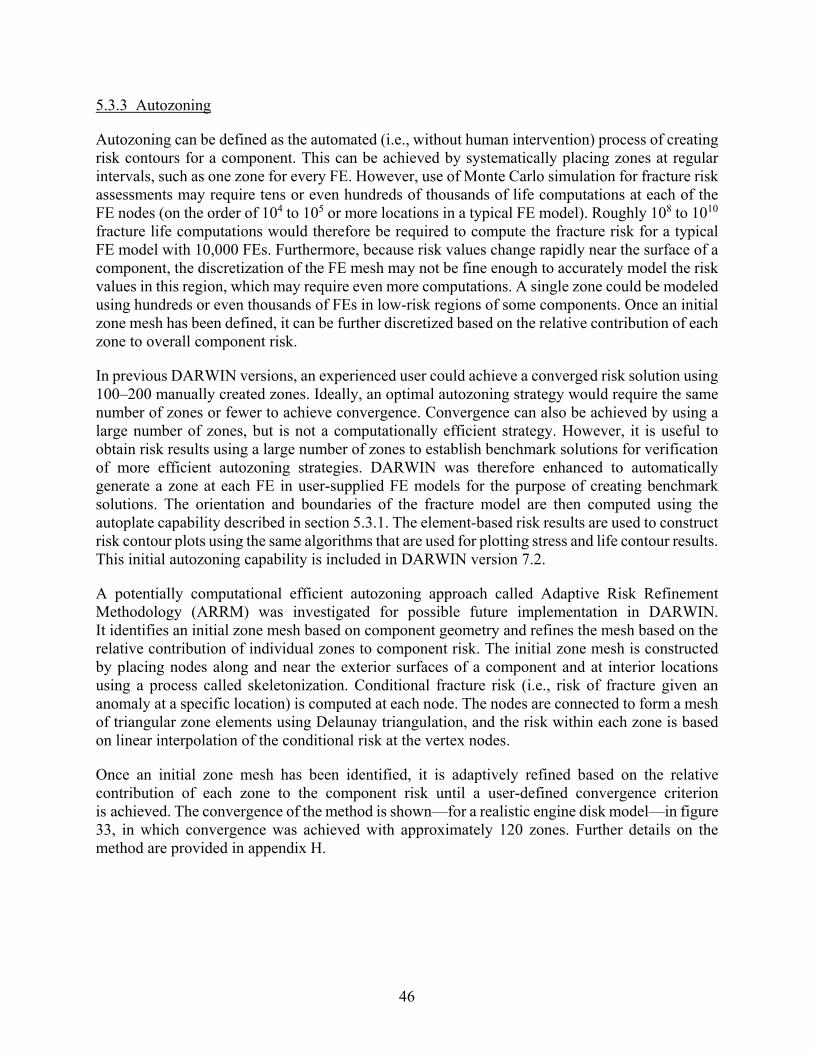
46

5.3.3 Autozoning

Autozoning can be defined as the automated (i.e., without human intervention) process of creating risk contours for a component. This can be achieved by systematically placing zones at regular intervals, such as one zone for every FE. However, use of Monte Carlo simulation for fracture risk assessments may require tens or even hundreds of thousands of life computations at each of the FE nodes (on the order of 104 to 105 or more locations in a typical FE model). Roughly 108 to 1010 fracture life computations would therefore be required to compute the fracture risk for a typical FE model with 10,000 FEs. Furthermore, because risk values change rapidly near the surface of a component, the discretization of the FE mesh may not be fine enough to accurately model the risk values in this region, which may require even more computations. A single zone could be modeled using hundreds or even thousands of FEs in low-risk regions of some components. Once an initial zone mesh has been defined, it can be further discretized based on the relative contribution of each zone to overall component risk.

In previous DARWIN versions, an experienced user could achieve a converged risk solution using 100–200 manually created zones. Ideally, an optimal autozoning strategy would require the same number of zones or fewer to achieve convergence. Convergence can also be achieved by using a large number of zones, but is not a computationally efficient strategy. However, it is useful to obtain risk results using a large number of zones to establish benchmark solutions for verification of more efficient autozoning strategies. DARWIN was therefore enhanced to automatically generate a zone at each FE in user-supplied FE models for the purpose of creating benchmark solutions. The orientation and boundaries of the fracture model are then computed using the autoplate capability described in section 5.3.1. The element-based risk results are used to construct risk contour plots using the same algorithms that are used for plotting stress and life contour results. This initial autozoning capability is included in DARWIN version 7.2.

A potentially computational efficient autozoning approach called Adaptive Risk Refinement Methodology (ARRM) was investigated for possible future implementation in DARWIN. It identifies an initial zone mesh based on component geometry and refines the mesh based on the relative contribution of individual zones to component risk. The initial zone mesh is constructed by placing nodes along and near the exterior surfaces of a component and at interior locations using a process called skeletonization. Conditional fracture risk (i.e., risk of fracture given an anomaly at a specific location) is computed at each node. The nodes are connected to form a mesh of triangular zone elements using Delaunay triangulation, and the risk within each zone is based on linear interpolation of the conditional risk at the vertex nodes.

Once an initial zone mesh has been identified, it is adaptively refined based on the relative contribution of each zone to the component risk until a user-defined convergence criterion is achieved. The convergence of the method is shown—for a realistic engine disk model—in figure 33, in which convergence was achieved with approximately 120 zones. Further details on the method are provided in appendix H.

47

Figure 33. Convergence of disk risk with increasing number of zones using the automated risk-refinement approach

5.3.4 GUI Redesign to Support Autozoning

As mentioned in section 5.3.3, DARWIN 7.2 includes an initial capability for automatic generation of zones for risk assessment of engine components containing inherent material anomalies. In previous versions of DARWIN, the user had to define zones one at a time. This involved selecting the FEs associated with a zone and then assigning component properties (e.g., anomaly distributions, material properties, inspection schedules) to the zone. Because autozoning involves automatic assignment of FEs and component properties to zones without user intervention, the relationship among FEs and component properties must be defined by the user prior to autozoning. In DARWIN 7.2, the user interface was enhanced to enable the analyst to assign component properties directly to FEs rather than zones (figure 34). Once the various properties have been assigned, DARWIN identifies the regions with unique properties, called “property regions” (figure 35).

The FE-centric assignment of component properties associated with this feature can also be applied to manual creation of zones. Once the properties are assigned by the user, DARWIN provides the capability to convert property regions into zones for application to manual zoning (figure 36).

DARWIN was also enhanced to provide risk contour plots for improved visualization of risk compared to risk contribution factor plots (figure 37).

1.0

1.5

2.0

2.5

3.0

40 60 80 100 120 140

Number of Mesh Nodes

Pre

dict

ive/

Act

ual C

umul

ativ

e P

OF Zone Method (64 Zones)

ARRM

48

Figure 34. The user interface was enhanced to enable the analyst to assign component properties directly to FEs rather than zones

Figure 35. DARWIN was enhanced to identify the regions with unique properties

The user then importsproperties from filesor DARWIN libraries

A color contour isdisplayed to indicateproperty assignments

The user selects a property type here

Property 1

Property 2

Unique Regions

49

Figure 36. DARWIN includes a capability to convert property regions into zones for use in manual zoning

(a) (b)

Figure 37. DARWIN was enhanced to provide risk contour plots for improved visualization of risk compared to risk contribution factor plots: (a) example risk contribution factor plot,

and (b) example risk contour plot

6. GENERAL DARWIN ENHANCEMENTS

A number of general enhancements were implemented in DARWIN to address the needs of the FAA, RISC, and DARWIN users. Several enhancements were completed to satisfy specific items in FAA ACs, including a special analysis mode for certification assessment of titanium HA anomalies for AC 33.14-1, and several capabilities for assessment of hole features outlined in AC

Property Regions Zones

50

33.70-2. Several numerical accuracy and speed improvements were implemented to address the increasing run times associated with the steadily growing number of features and file sizes associated with the continuing development of DARWIN and its expanding role within original equipment manufacturers (OEM) organizations. DARWIN was also enhanced to provide treatment for general user needs such as large FEMs and DARWIN models with large numbers of zones. This section provides a summary of these enhancements.

6.1 DIRECT SUPPORT FOR IMPLEMENTATION OF ACS

DARWIN was enhanced to improve its use for certification assessments associated with FAA ACs. For example, a special analysis mode was implemented for certification assessment of titanium HA anomalies covered in AC 33.14-1. DARWIN was also enhanced to provide several capabilities for assessment of hole features outlined in AC 33.70-2, including user specification of manufacturing process credits, an FAA hole feature surface damage report form, and a special analysis mode for certification of hole features.

6.1.1 Special Analysis Modes for Certification Assessments

To guide users in the selection of the appropriate analysis options, DARWIN was enhanced so that all of the analysis modes (for both inherent anomalies or surface damage) were redefined as either “General” or “FAA Certification.” When the user selects the “General” analysis mode (figure 38(a)), the user has access to all of the DARWIN capabilities for assessment of components with either inherent or surface damage anomalies. For certification calculations, the user selects the “FAA certification” analysis mode (figure 38(b)), which restricts the user to the anomaly types and analysis methods that are currently addressed by FAA ACs 33.14-1 and 33.70-2. This feature was first released in Version 6.1.

(a) (b)

Figure 38. Redefined DARWIN analysis modes: (a) “general” analysis mode, which provides access to all of the DARWIN capabilities and (b) “FAA certification” analysis

mode, restricted to the DARWIN anomaly types and analysis methods currently addressed by FAA ACs 33.14-1 or 33.70-2

51

6.1.2 AC 33.70-2 for Hole Features

6.1.2.1 User Specification of Manufacturing Process Credits for Hole Features

FAA AC 33.70-2 Appendix 6 describes a number of manufacturing credits associated with applicable process controls that can be applied to potentially reduce the fracture risk of a component. The AC provides an approach to take credit for company-specific enhancements to the hole-making process that can be directly applied to computation of hole feature risk. A summary of the manufacturing credits in the AC is indicated in table 1.

Table 1. Summary of manufacturing process controls and associated credit factors

Process Control Definition

Credit Factor

Process Validation

A procedure in which it is demonstrated that the Manufacturing Process delivers parts consistent with the Design Intent (see FAA Report Number DOT/FAA/AR-06/3). Process validation is understood in this AC to include an inspection of the part for geometric anomalies (cracks, scratches, dents, scores, etc.) after manufacture. Such an inspection may be visual, enhanced visual, or semi-automatic, such as ECI.

5

Single Point Boring

The removal in a finishing operation of a small depth of material, at least 0.004" deep, in the bore of the hole by use of a single-point boring tool. This credit is allowed for titanium alloys only.

5

Honing The removal of a small depth of material, at least 0.002", by a self-centering grinding operation. This credit is allowed for all materials.

5

Coolant Monitor

A device that ensures a continuous flow of coolant with periodic checks on the pressure and the concentration of the coolant supplemented with the training of operators to ensure the direction of the flow toward the cutting edge (see FAA Report number DOT/FAA/AR-06/3). This credit is allowed for all materials.

5

Power Monitor

A device that continuously monitors the power consumed by the machine tool and which must be shown to be sensitive to such conditions as worn tools, loss of coolant, etc., which give rise to anomalies (see FAA Report Number DOT/FAA/AR-06/3). This credit is allowed for all materials.

For the use of either a power monitor or a feed force monitor, 20. For the use of both a power monitor and a feed force monitor, 30.

Feed Force Monitor

A device that continuously monitors the feed force used by the machine tool and which must be shown to be sensitive to such conditions as worn tools, loss of coolant, etc., which give rise to anomalies (see FAA Report Number DOT/FAA/AR-06/3). This credit is allowed for all materials.

Inspection

In this context, inspection is confined to the use of inspection techniques specifically aimed at detecting nongeometric anomalies, such as highly distorted material, smeared material, white or amorphous layer (see FAA Report Number DOT/FAA/AR-06/3). Generally, this would be an etch inspection specifically targeted at the hole and which must be shown to detect such anomalies. This credit is allowed for all materials.

5

52

When process controls are used, the unconditional probability of fracture of a component is divided by the credit factor indicated in this table. Manufacturing credits can be applied for multiple process controls, where the total manufacturing credit is equal to the sum of the credits for the individual processes. Note that some limitations exist regarding credits for multiple processes (see AC 33.70-2 Appendix 6 note 2 for further details). A DARWIN capability was implemented beginning with Version 7.0 to enable the user to specify manufacturing process credits for surface damage assessments, as shown in figure 39. The credits are applied to probability of fracture values using the approach described in AC 33.702.

Figure 39. DARWIN GUI screens for user specification of manufacturing process credits

53

6.1.2.2 FAA Hole Feature Surface Damage Report Form

DARWIN provides the capability to prepare forms for a concise summary of analysis results that would be appropriate for submission to the FAA in support of the certification process. In previous versions, this capability was limited to titanium HA assessments. Under this project, this capability was extended to generate report forms for surface damage assessment, as described by AC 33.70-2. The content and format of the form were based on guidance from RISC. The form includes the essential assessment data that would be applicable for an FAA review. The FAA Hole Feature Surface Damage Report Form is shown in figure 40. This feature was introduced in Version 7.0.

54

Figure 40. FAA hole feature surface damage report form implemented in DARWIN 7.0

55

6.1.2.3 FAA Certification Mode for Hole Features

In recent years, several DARWIN capabilities were developed to support RISC activities related to assessment of surface damage in various forms (e.g., hole features, turned surfaces, blade slots). Damage-tolerance analysis of hole features in high-energy turbine engine rotors is described in FAA AC 33.70-2, but ACs have not yet been published for the other surface damage capabilities in DARWIN. As noted previously, a special analysis mode was created for FAA certification purposes that restricts the DARWIN surface damage capabilities to assessment of hole features. When this analysis mode is activated, it prevents the user from selecting 2D FEMs (typically used for assessment of turned surfaces), and total disk risk results are presented only for the highest risk feature (zone). This feature was introduced in DARWIN 6.1.

6.2 FE2NEU TRANSLATOR

The FE2NEU FE results translator (figure 41) was developed to convert ANSYS FE results to the neutral file format required by DARWIN. FE2NEU replaced the previous translator (ANS2NEU), which consisted of portions of the SIESTA code previously provided by GE. The translator, introduced in Version 6.1, was developed using a combination of funds from the current project and DARWIN licensing funds.

Figure 41. Overview of FE2NEU FE results translator

The FE2NEU translator supports all of the FE types that were previously supported by ANS2NEU (table 2). It also provides filtering capabilities that are identical to those found in ANS2NEU (i.e., include/exclude certain load cases or elements based on element type, element number, material number, or load case number). The input/output format of FE2NEU is very similar to ANS2NEU and can be called directly by the GUI without significant modifications.

Table 2. FE types supported by FE2NEU

ANSYS Type SIESTA Type Comment

PLANE42 EL2D 4-node quadrilateral

PLANE82 PE2D 8-node quadrilateral

SOLID45 BRI8 Brick or prism

SOLID92 TETS N10 10-node tetrahedron

SOLID95 VANS N20 Brick, prism, or pyramid

56

FE2NEU includes several important features that previously were not available in ANS2NEU. It supports ANSYS version 10 files (and also previous ANSYS versions). FE2NEU provides support for large ANSYS results files (successfully tested for several large files, including a 1.5 GB file with 953226 PLANE82 elements). It allows the user to specify filter commands on a single (200-character) line (ANS2NEU requires multiple lines) and provides output with nodes and elements sorted in ascending order.

FE2NEU is also computationally efficient. For example, FE2NEU completed translation of a 242 MB file in 6.5 seconds, compared to 620 seconds required by the version of ANS2NEU previously available to SwRI (see figure 42). Translation time for large files is also brief (FE2NEU translation time for a 1.5 GB file with nearly 1 million elements was completed in 37 seconds).

Figure 42. Examples of reduction in the time required to convert an ANSYS file to the DARWIN neutral file format using FE2NEU vs. ANS2NEU

FE2NEU was developed with future maintenance in mind. Unlike ANS2NEU, which consists of hundreds of subroutines (more than 100,000 lines of code) written in an outdated programming language (FORTRAN77), FE2NEU consists of only a few primary modules that use advanced FORTRAN90 features (e.g., dynamic memory allocation, derived types) for efficient storage and retrieval of data.

Most FEMs have a large number of elements, making it difficult to identify and list the element numbers that need to be filtered. An element filter was developed in FE2NEU that allows the User to filter FEMs based on element groupings called Named Components. Named Components are defined in the ANSYS Named Component definition file provided by ANSYS (the User can obtain this file by issuing the command “CMWRITE” during an ANSYS session). The Named Components may consist of nodes, elements, lines, areas, and volumes, but only the element-type is used for element filtering in FE2NEU. An example Named Component definition file is shown in figure 43.

0

100

200

300

400

500

600

700

0 400 800 1200 1600

ANSYS result file size (MB)

Co

nvers

ion

tim

e (seco

nd

s)

ANS2NEU

FE2NEU

57

Figure 43. An example ANSYS named component definition file

Figure 44 shows the FE2NEU element filtering process using Named Components. The User first generates the ANSYS FE results file (*.rst file) and ANSYS Named Component definition file (*.cdb file) during an ANSYS session. Next, the User loads the results file into the FE2NEU GUI and selects the associated Named Component definition file. FE2NEU parses the Named Component file and displays all available components. The User selects the Named Components to include or exclude in the output model (figure 45). FE2NEU then translates the results file to the DARWIN neutral file format (*.uif, *.uof) and filters the model based on the elements associated with the Named Components. Note that additional filtering criteria (e.g., material, element numbers, load case numbers) can be applied in conjunction with the Named Components filter.

FE2NEU was also enhanced to provide support for translation of ABAQUS models to the DARWIN neutral file format. With the exception of the Named Components capability, all the filtering features developed for translation of ANSYS models are directly applicable to translation of ABAQUS models. Development of this additional translation capability was supported by DARWIN licensing funds, and it was first released in DARWIN 7.0.

58

Figure 44. The FE filtering process using ANSYS named components

Figure 45. Selection of named components filter in FE2NEU

59

6.3 IMPROVEMENTS FOR GENERAL INHERENT ANOMALIES

DARWIN was originally developed specifically to address the HA threat and to support the corresponding FAA AC 33.14-1. However, as DARWIN evolved, new features were added to address other types of inherent anomalies. These new features, introduced in DARWIN 6.0, included (1) fully 3D anomalies that are defined using six random variables, (2) production inspections and associated POD curves that can be used to simulate a manufacturing inspection that is performed before a component is placed in service, and (3) a crack formation module to simulate a nonzero crack formation period and associated scatter.

For general inherent anomalies with nonspherical shapes, the cross-sectional area detected using available inspection techniques is dependent on the orientation of the anomaly relative to the inspection plane, and on the associated footprint of the anomaly in the inspection plane. Two configurations were implemented in DARWIN 6.0 to model the footprint of the anomaly in the inspection plane: (1) intersection and (2) projection. For the intersection approach (figure 46), the footprint is defined as the area of the intersection of the anomaly and an inspection plane that passes through the center of the anomaly. For the projection approach (also shown in figure 46), the footprint is based on the projection of the exterior anomaly surface on the inspection plane.

Figure 46. Two configurations were identified to model the area of a general inherent anomaly detected using available inspection techniques: (1) intersection and (2)projection

6.4 SPEED AND ACCURACY IMPROVEMENTS

Over the course of this project, the number of features in DARWIN has substantially increased. Computational efficiency improvements were necessary to ensure that users can continue to perform DARWIN assessments within a reasonable amount of time. Numerical accuracy improvements were also implemented as needed to support new features and address bugs.

60

6.4.1 Parallel Processing

A new parallel processing capability was implemented in DARWIN 7.2 that automatically distributes the risk-assessment code computations to multiple central processing units (CPUs) on a single computer. The capability was implemented using the OpenMP approach that is ideally suited for parallel processing on a single multicore computer. From the user’s perspective, execution of the parallel version is identical to the previous (serial) version. It does not require installation of extra files or execution of script files. The parallelization was applied at the zone level in which all of the computations associated with an individual zone are performed by a single processor, and multiple zones can be applied to different processors. This approach enables accelerated computations for nearly all analysis modes, including stress processing, deterministic crack growth life assessment, risk assessment, life contours, and auto-zoning.

The parallel-processing capability can substantially reduce the computation time required for risk-assessment computations. As shown in figure 47, computation speedup factors for risk assessment of a typical gas turbine engine disk were on the order of 4X – 6X when using a single computer with eight processors. Runtime speedup factors are shown for the three probabilistic simulation methods in DARWIN, including Monte Carlo simulation, Monte Carlo simulation using the LAF approach (Monte Carlo w/LAF, described in section 6.4.7), and importance sampling. The DARWIN GUI was enhanced to enable the user to specify the number of processors to be applied to parallel processing computations (figure 48).

A dynamic load-balancing approach was used to efficiently distribute the computational workload among the various CPUs. Unlike the static approach in which computational processes are evenly distributed among CPUs, the dynamic approach distributes processes based on computation time. The computation times can differ substantially from zone to zone, so this approach can provide significant time savings compared to the static approach.

Prior to Version 7.2, zone risk computations were performed sequentially (i.e., one zone after another) and the results were dependent on the sequence in which the zone computations were performed. This approach was sufficient for the serial version because the zone computations were always performed in the same sequence. However, because the sequence can vary considerably for the parallel version, this approach could no longer be used. To address this issue, a new random number generator, known as RNGStreams [29], was implemented, which generates a stream of random numbers that can be subdivided into multiple sub-streams for application to parallel processing. The sub-streams of random numbers are assigned to zones and samples based on the zone and sample numbers independent of the order in which they are processed. This approach guarantees that the risk results are identical for each zone from run to run, regardless of the number of processors that are used.

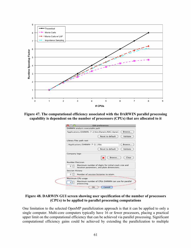
61

Figure 47. The computational efficiency associated with the DARWIN parallel processing capability is dependent on the number of processors (CPUs) that are allocated to it

Figure 48. DARWIN GUI screen showing user specification of the number of processors (CPUs) to be applied to parallel processing computations

One limitation to the selected OpenMP parallelization approach is that it can be applied to only a single computer. Multi-core computers typically have 16 or fewer processors, placing a practical upper limit on the computational efficiency that can be achieved via parallel processing. Significant computational efficiency gains could be achieved by extending the parallelization to multiple

62

computers. High-performance computer clusters may consist of hundreds or even thousands of computers with up to 16 processors each. However, this requires sophisticated communication among the computers, which can usually be achieved only by using some form of MPI-based parallelization. The MPI-approach uses a distributed memory scheme in which data cannot be shared among multiple processes that have common variables. As a result, the available memory of each computer within the cluster can become the limiting factor for the parallelization.

An initial investigation was performed under this project to develop a prototype parallel version of DARWIN that combines the shared memory capability of the OpenMP approach with the multi-computer capability of the MPI approach. In the prototype software, the MPI library was used to identify the number of available processors associated with each computer within a cluster, distribute zone input data to each computer based on the number of processors (distributed memory), and execute the risk-assessment code on each computer. Thereafter, the zone computations were automatically distributed to the available processors within each computer, and the input data were shared among these processors using the previously developed OpenMP approach. Preliminary results suggest that computation times may be substantially reduced without a significant increase in memory usage for any single computer. Further study is required to identify any potential limitations of this approach.

6.4.2 Enhanced Restart Algorithm

A new algorithm was implemented in DARWIN 6.1 that reduces the data-retrieval time associated with restart operations. Previously, the information in the database files was retrieved on a zone-by-zone basis, requiring multiple file access operations (open, parse, search, read, close). The new algorithm stores all information associated with a database file in memory for later use, significantly reducing the number of file-access operations. A comparison of the number of file-access operations associated with the previous and new algorithms is shown in table 3.

Table 3. File access operations associated with DARWIN 6.0 and 6.1 restart algorithms

Restart Algorithm

Open, Parse, and Close Operations Search Operations

Minimum Maximum Minimum Maximum

DARWIN 6.0

DARWIN 6.1

Note: n = number of zones; m = number of database files

nm

2

1mn / 1

2

n n m 2

1nn

m 12 m n

2

1nn

63

6.4.3 Treatment of Shakedown With Stress Scatter

DARWIN includes a module called SHAKEDOWN that converts the results of a linear elastic stress analysis into an approximate elastic-plastic stress distribution by calculating residual stresses resulting from stress relaxation and redistribution due to local plastic deformation. Prior to DARWIN 7.0, shakedown was applied to the maximum deterministic stress value before risk assessment, and the relaxed stress values for all load steps were based on this deterministic residual stress result. Because random stress results are based on the product of the relaxed stress and the stress scatter factor, this approach provided conservative risk results when stress scatter was invoked and stress values exceeded the yield stress.

In Version 7.0, DARWIN was enhanced to perform shakedown during risk assessment when both shakedown and stress scatter options are selected. Because the shakedown process requires significant computational effort, it would be impractical to apply it for every sample in the risk computation. Instead, it is applied only when the maximum stress along the crack growth path exceeds the yield stress (see shaded area in figure 49). If the deterministic maximum stress is far smaller than the yield stress, there will be relatively few (if any) cases in which the scaled maximum stress is greater than the yield stress during the risk-sampling process. The number of shakedown computations is dependent on the relative magnitudes of deterministic maximum stress, yield stress, and stress scatter distribution.

Figure 49. Stress scatter distribution and yield stress ( )

6.4.4 Crack Growth Life Interpolation Enhancement

The DARWIN Flight_Life crack growth life integration algorithm determines the optimal crack growth life-cycle increments (or integration steps/points) to obtain crack propagation life efficiently for a specified precision. The optimal cycle increments usually do not contain all cycle values needed for user-specified result printing and inspection schedules. Prior to Version 7.0, the cycle values at user-specified print/inspection intervals were added to the integration points of the Flight_Life method to obtain results at these cycles. Consequently, the Flight_Life results were influenced by user-specified print/inspection intervals because the numerical integration result was dependent on the number of integration steps.

0.00

0.05

0.10

0.15

0.20

0.25

Stress

Pro

bab

ility

den

sity

y

Deterministic max stress

y

64

An interpolation method was implemented in DARWIN 7.0 to address this issue. The new method uses a nonintrusive approach consisting of two steps. First, the crack-growth life is calculated based on the optimal cycle increments determined by the Flight_Life integration algorithm. Then the results at user-specified print/inspection intervals are obtained from an interpolation of crack-growth life results, as shown in figure 50. Consequently, the results are more consistent because the integration steps are not affected by the user-specified print/inspection intervals.

Figure 50. Flight_life results based on optimal cycle increments and the interpolated results at user-specified print intervals

6.4.5 Enhanced Mesh Generation Algorithm

DARWIN includes a mesh generation algorithm that creates a thin layer of FEs along the surface of an FE geometry to model near-surface embedded anomalies (the so-called “onion skin”). Prior to Version 7.0, the mesh-generation algorithm was based on a translation of surface line segments. This approach introduced small discontinuities in the mesh (figure 51) that could influence the accuracy of GUI contour plots. To resolve this problem, an enhanced mesh algorithm was developed in DARWIN 7.0 that is based on translation of nodes and re-meshing of adjacent FEs. The algorithm first creates nodes along edges attached to the border and removes any nodes that overlap (e.g., where two line segments meet). These nodes are then translated into the component along the interior edges of the surface Fes, based on the value of the onion-skin depth (supplied by the user) and define the boundary for subdivision of the surface elements. The nodes are also used to define the boundary for subdivision of adjacent elements. For some geometries, several different meshes can be formed from the nodes during the subdivision process. In this situation, the GUI selects the final mesh based on the mesh configuration that maximizes the area-to-circumference ratio of the resulting FEs.

0.010

0.011

0.012

0.013

0.014

0.015

0.016

0 1000 2000 3000 4000 5000

Loading Cycles (N)

Cra

ck

Siz

e (

a)

User-specified print intervals

Optimal cycle increments

65

Figure 51. Mesh discontinuities introduced by the previous DARWIN mesh-generation algorithm

An illustrative example of onion-skin mesh generation using the enhanced algorithm is shown in figure 52. The previous algorithm (figure 52(b)) did not support triangular elements. The new algorithm provides treatment for triangular elements and resolves the associated discontinuities (figure 52(c)). The new algorithm also enhances the element-refinement process and permits construction of onion skins along boundaries with single displaced elements protruding from an otherwise smooth surface. The new algorithm provides an improved mesh that is useful for the life contour and autozoning features.

Figure 52. Example of onion-skin mesh generation: (a) unrefined mesh, (b) previous mesh generation algorithm (DARWIN 6.1), and (c) new mesh generation algorithm

(DARWIN 7.0)

6.4.6 Computational Speed Improvement for Critical Anomaly Size Computation

DARWIN uses a bisection method to determine the critical anomaly size for a given target life. For each target-life value, DARWIN initiates the search by computing the life values of the smallest and largest anomaly sizes in the anomaly distribution, and then continues the search using bisection computing lives until the critical anomaly size is found. The computation time required to identify the critical anomaly size is determined primarily by the number of life calculations in the bisection search. Prior to Version 7.0, an independent life calculation was required at each step of the bisection search.

66

DARWIN 7.0 was enhanced to store the intermediate life values in memory (caching table) that are computed during the bisection search process. For the first critical anomaly size, the life values and anomaly sizes obtained during the search are stored in the table. For each subsequent critical anomaly size, DARWIN first searches the caching table to locate the smallest range of anomaly sizes that encompass the target life and then performs bisection iteration within that range. As a result, DARWIN only needs to search from the smallest and largest anomaly sizes for the first critical anomaly size computation. The search range becomes narrower and the associated number of life computations is reduced as additional life results are saved in the cache table. Initial studies indicate that the enhancement results in a 50% reduction in the time required to perform the critical anomaly size computation.

6.4.7 Accuracy Improvement for LAF Method

The LAF method is a response surface method that creates an array (LAF table) of deterministic life and associated crack area values for a family of initial anomalies. For reliability computations, random anomaly sizes are obtained using Monte Carlo simulation, and the associated life and crack areas are interpolated from the LAF table. Crack area values are needed to construct the LAF table, but the crack-growth algorithm (Flight_Life) does not report them at regular intervals. Prior to Version 7.1, the crack areas in the LAF table were computed at fixed intervals by interpolating over the crack areas at nearest cycles in the output of the crack-growth module. Some precision was lost as a result of this interpolation. The LAF method was improved in DARWIN 7.1 by adjusting the LAF table intervals to match the reporting intervals of Flight_Life. This not only improved the accuracy of the LAF method, but also slightly improved efficiency by eliminating the interpolation previously required to construct the LAF table.

6.4.8 Computational Speed Improvements Associated With New Fortran Compiler

A computational speed improvement was recently achieved by selecting a new Fortran compiler (Intel® Visual Fortran) and adjusting the compiler options for optimum performance. Prior to Version 7.1, the Compaq Visual Fortran Compiler was used for the Windows® platform, and G95 was used for the Linux and Mac® OS X platforms. Based on a number of studies, it was determined that the Intel Fortran compiler used for compiling DARWIN beginning with Version 7.1 provided significant speed improvements compared to the other compilers. Verification test results indicated approximately 2 speed improvement compared to the previous DARWIN 7.0 release. Moreover, because the Intel compiler can be used on all supported platforms, it substantially simplified the software verification and release processes.

6.4.9 Computational Speed Improvements Due to Representation of Text Strings

The DARWIN Fortran source code was enhanced so that selected text input data were represented as integers rather than as text strings. This improvement, implemented in Version 7.1, resulted in a 15% speedup in execution time for all supported platforms.

6.5 STRESS PROCESSING ENHANCEMENTS

Stress processing enhancements were implemented to support new features and to improve the computational efficiency of existing capabilities. Two algorithms were developed to improve the

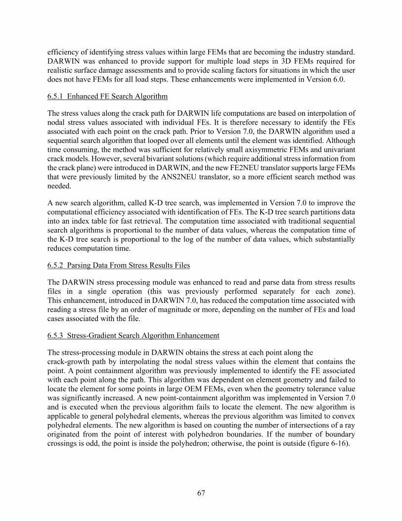
67

efficiency of identifying stress values within large FEMs that are becoming the industry standard. DARWIN was enhanced to provide support for multiple load steps in 3D FEMs required for realistic surface damage assessments and to provide scaling factors for situations in which the user does not have FEMs for all load steps. These enhancements were implemented in Version 6.0.

6.5.1 Enhanced FE Search Algorithm

The stress values along the crack path for DARWIN life computations are based on interpolation of nodal stress values associated with individual FEs. It is therefore necessary to identify the FEs associated with each point on the crack path. Prior to Version 7.0, the DARWIN algorithm used a sequential search algorithm that looped over all elements until the element was identified. Although time consuming, the method was sufficient for relatively small axisymmetric FEMs and univariant crack models. However, several bivariant solutions (which require additional stress information from the crack plane) were introduced in DARWIN, and the new FE2NEU translator supports large FEMs that were previously limited by the ANS2NEU translator, so a more efficient search method was needed.

A new search algorithm, called K-D tree search, was implemented in Version 7.0 to improve the computational efficiency associated with identification of FEs. The K-D tree search partitions data into an index table for fast retrieval. The computation time associated with traditional sequential search algorithms is proportional to the number of data values, whereas the computation time of the K-D tree search is proportional to the log of the number of data values, which substantially reduces computation time.

6.5.2 Parsing Data From Stress Results Files

The DARWIN stress processing module was enhanced to read and parse data from stress results files in a single operation (this was previously performed separately for each zone). This enhancement, introduced in DARWIN 7.0, has reduced the computation time associated with reading a stress file by an order of magnitude or more, depending on the number of FEs and load cases associated with the file.

6.5.3 Stress-Gradient Search Algorithm Enhancement

The stress-processing module in DARWIN obtains the stress at each point along the crack-growth path by interpolating the nodal stress values within the element that contains the point. A point containment algorithm was previously implemented to identify the FE associated with each point along the path. This algorithm was dependent on element geometry and failed to locate the element for some points in large OEM FEMs, even when the geometry tolerance value was significantly increased. A new point-containment algorithm was implemented in Version 7.0 and is executed when the previous algorithm fails to locate the element. The new algorithm is applicable to general polyhedral elements, whereas the previous algorithm was limited to convex polyhedral elements. The new algorithm is based on counting the number of intersections of a ray originated from the point of interest with polyhedron boundaries. If the number of boundary crossings is odd, the point is inside the polyhedron; otherwise, the point is outside (figure 6-16).

68

Figure 53. Point-containment test algorithm

6.5.4 Multiple Load Steps for 3D Models

The DARWIN 3D surface-damage assessment capability was extended in DARWIN 6.1 to address FEMs with multiple load steps to support RISC bolt-hole surface-damage activities. This analysis mode had been previously limited to FEMs with a single load step.

6.5.5 Mission Scaling Factor Enhancements

A new mission scaling mode called “Absolute” was developed in DARWIN 6.1 to support OEM regression models (figure 54). In the Absolute mode, the user can specify stress and temperature values at the initial crack location for all zones within a specified zone group.

Figure 54. “Absolute” mission scaling mode implemented in DARWIN GUI

The stress and temperature values in each zone are multiplied by the ratio of the specified absolute values to the FE stress and temperature values at the crack location in the zone:

(8)

(9)

where and are stress and temperature values at the initial crack location (from FEA results), and are stress and temperature values at any location (from FEA results), and

are user-specified stress and temperature values.

x x xP0

x x xP0

givenFE

crack

givenFE

crack

TT T

T

crack crackT

FE FET

given givenT

69

In contrast, the mission scaling factors in the previously available “Scale” mode are multipliers that are applied to stress and temperature values:

(10)

(11)

where and are the user-specified stress and temperature scaling factors, respectively. In the “Scale” mode, the final stress and temperature values associated with a given load step are obtained by multiplying the stress and temperature values from FEA by their respective scaling factors.

6.6 DATABASE AND FILE-MANAGEMENT ENHANCEMENTS

A number of database and file-management enhancements were performed to address the increasing amount of data associated with DARWIN assessments. The DARWIN input and output files were converted to an Extensible Markup Language (XML) format for improved efficiency and error reduction, and verbosity controls were introduced to enable the user to control the amount of data printed to output files. Additional information was also provided for RISC & Steering Committee assessments and for verification checks.

6.6.1 XML Input File/Text Editor

Prior to DARWIN 6.0, a plain text input file (*.DAT) format was used for the Fortran code which required parsing of the input file. This approach was inefficient and prone to errors. It was estimated that more than 40% of the bugs associated with the code-development process could be attributed to errors associated with parsing of the input file. Furthermore, the data from the GUI were in a different format (*.XML), which had to be translated to the plain text format prior to execution of the risk-assessment code. The GUI had to support both file formats, and two data structures had to be designed whenever a new feature was implemented in DARWIN.

The Fortran code was enhanced to use the GUI XML data format directly. The XML format includes rigorous error checking, which can potentially reduce the number of bugs related to input file processing. Moreover, the use of a single file format for both the GUI and Fortran code completely eliminates the translation errors associated with the two-file format approach.

One of the advantages of the previous plain text format was that it allowed users to manually edit text files easily prior to execution of the risk assessment code. The XML format is efficient for computer processing but unfortunately is difficult to edit in a standard text editor. However, this format is actually easier to edit when viewed in a text editor that supports XML files. As shown in figure 55, an XML editor was implemented in DARWIN 6.0 that enables the user to view and edit XML-based input files. The editor displays the data in a tree-like structure that allows the user to expand and collapse complete data fields, which is very useful for browsing large input files. The editor supports data copying, pasting, and insertion, which are essential for text editing operations.

FE f

FE TT T f

f Tf

70

Figure 55. XML editor implemented in DARWIN that enables the user to view and edit XML-based input files

6.6.2 Managing Large Files

Prior to DARWIN 7.0, the results were written to two files: ASCII format (*.out) and XML format (*.ddb). The *.out file is in a plain-text format that is readable by the User, and the *.ddb file is intended for the GUI. In addition to deterministic fracture mechanics and risk results, these two results files also contain intermediate results, such as stress gradients and material properties at various temperatures. For large models with many load steps, the results files can become extremely large and may be impractical to view in the GUI. Furthermore, some users may not be interested in the intermediate results and may prefer smaller output files to save disk space. To address these needs, a new output verbosity control was implemented in DARWIN 7.0 to allow the User to select specific portions of results to be written to output files shown in figure 56. For instance, instead of outputting a full stress field, the User can choose to output a compact stress field (maximum 10 points in one dimension), to output the stress at the crack only, or to completely turn off the stress field output altogether. This can be very useful, especially for bi-variant stress fields that consist of 100 by 100 matrices in full output format. With this new feature, the user also has the option to completely turn off *.ddb and/or *.out files.

71

Figure 56. DARWIN output verbosity control settings

The user may specify the output options using one of four predefined output modes: “Off,” “Compact,” “Full DDB only,” and “Full” modes (figure 57). For example, in the “DDB Only” mode, the *.out file is completed turned off and the *.ddb file is written in full format.

Figure 57. DARWIN output verbosity predefined output modes

6.6.3 Additional Output for Deterministic Crack Growth Assessments

Prior to DARWIN 7.1, deterministic fracture mechanics results were limited to summary values, such as the number of cycles to failure, the crack size (area, length, depth) versus flight cycles, and the maximum SIF (Kmax, without beta correction) among all crack tips versus flight cycles. The Steering Committee requested that additional output data be provided to support verification and

72

validation activities. A new capability was implemented in DARWIN 7.1 that provides detailed crack state information at the intra-mission load pair level. A summary of the variables provided is shown in table 4.

Table 4. Summary of deterministic output variables available in DARWIN

Data Type Description

Cycle Crack growth integration increments in terms of number of flights

Pair Stress pair ID

a Crack depth

c Crack length

a/c Crack aspect ratio

xd Crack center location along local x-axis

zd Crack center location along local z-axis

Kmaxi SIF associated with the maximum load case in the stress pair

Kmini SIF associated with the minimum load case in the stress pair

Kopeni

SIF including the effect of the Newman’s crack closure function. Kopen = Kmax ƒ where f is the Newman closure function. Kopen is used to compute the effective SIF range for analyses using the Closure stress ratio model.

Kplasi

An adjustment of the maximum SIF (Kmax) that includes a plastic zone-size correction. It is enforced only when Kmax exceeds 90% of the fracture toughness. Note: Kplas is used only for failure checking.

BCFi Known as the beta correction factor, it is a correction factor for surface-breaking crack tips that is applied to the SIF range (dKapp).

dKappi

SIF range dKappi = K = [Kmax]i – [Kmin]i Note: The provided values do not include the effect of the beta correction factor.

73

Table 4. Summary of deterministic output variables available in DARWIN (continued)

Data Type Description

dKeffi

Known as the effective SIF range, it is the adjusted SIF range that includes stress-ratio effects. It applies specifically to analyses that incorporate the Walker Equation or Closure stress ratio models. dKeff = U dKapp

where for the Closure stress ratio model.

da/dN Average crack growth rate of a+ and a- crack tips

dc/dN Average crack growth rate of c+ and c- crack tips

RKi Stress ratio based upon SIFs RKi = Kmini/Kmaxi

GFi

The geometry factor includes the effects of geometric considerations and an applied stress. GF = where σ is an applied stress (i.e., a remote stress) and β is a geometric factor. Therefore, the classical K equation is given by:

where a is the crack depth designated in the hx direction. Note: For a uniformly distributed stress gradient, the value of the applied stress σ is equal to the stress at the crack tip. However, for a non-uniformly distributed stress gradient, the values of the applied stress and crack-tip stress are not equal.

Note that the additional data are primarily for verification and validation activities and do not need to be provided for day-to-day DARWIN assessments. This capability was therefore implemented as a user option that appears in the DARWIN Output Verbosity Menu (figure 57). When this feature is enabled, DARWIN writes an additional output file containing the additional deterministic variables (a sample output file is shown in figure 58).

√ GF

74

Figure 58. A sample DARWIN deterministic output data file (NOTE: the index numbers “1, 2, 3, 4” following “Kmax” indicate the respective crack tips)

6.6.4 Verification Checks and Keywords

A number of additional verification checks were implemented in the DARWIN GUI and risk assessment code in Version 6.0 to ensure that anomaly distributions and POD curves were correctly applied to the crack types and analysis modes that are available in DARWIN. To enforce these checks, a number of new keywords were created for the DARWIN anomaly distribution and POD curve files and are required for successful execution. A summary of these keywords is provided in the DARWIN User’s Guide.

The keywords provide an added level of verification checking of DARWIN input data files. However, input files created using versions of DARWIN earlier than 6.0 do not include the keywords, and cannot be executed in the 6.0 or later versions. A GUI keyword conversion editor was therefore developed to help the user add the required keywords to input files from previous DARWIN versions for compatibility with later versions.

6.7 USER INTERFACE ENHANCEMENTS

DARWIN enhancements were implemented to enable the user to filter the display of warning messages and to view the list of optional features for a GUI session.

6.7.1 Filtering of GUI Warning Messages

The DARWIN GUI includes a feature to check for errors in the input file and provides a list of all error/warning messages. Users may wish to avoid the display of repeated trivial warning messages because these can sometimes occur in such large numbers that truly critical warnings go unnoticed. To address this issue, a warning filter was implemented in Version 7.0 that allows the user to specify the warnings that will appear in the GUI error/warning report. Filter activation and the associated user interface are shown in figure 59.

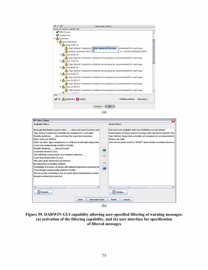
75

(a)

(b)

Figure 59. DARWIN GUI capability allowing user-specified filtering of warning messages: (a) activation of the filtering capability, and (b) user interface for specification

of filtered messages

76

6.7.2 GUI Display of Optional Features

Some of the features that have been implemented in DARWIN are not intended for all users. These features are normally hidden from view, but can be activated by entering the feature name and a special password that is unique to each feature. A GUI capability was implemented in DARWIN 7.0 that allows the user to view active optional features that are available in DARWIN. This capability, called “show active optional features” is located in the GUI tools menu, and is shown in figure 60.

Figure 60. DARWIN GUI capability allowing the user to view active optional features available in DARWIN

7. DARWIN TESTING AND EVALUATION

This task was focused on the formal testing and evaluation of the DARWIN software. New DARWIN versions were evaluated by both the primary developer (SwRI) and the engine companies. DARWIN was first tested internally using automated algorithms that were developed specifically for this purpose. The software was then provided to the engine companies for review via major software releases that occurred approximately once a year. These companies validated DARWIN against their own company codes, fleet experience, and test data. Upon verification, the software was released for use by licensed DARWIN users.

77

7.1 DARWIN CODE RELEASES

DARWIN development was performed throughout the project with major software releases occurring roughly once a year. For each major release, one or more initial (Alpha) versions were submitted to the Steering Committee for a review period lasting at least 3 months. During the review period, the Steering Committee provided feedback regarding the accuracy and usability of the software, and this feedback was addressed by SwRI. Immediately following the Alpha review period, a Beta version was released to RISC for review. During the Beta review period (at least 3 months), RISC provided additional feedback, which also was addressed by SwRI. Following these reviews, a final Production version was released to licensed users. A summary of the features associated with the major software releases is provided in this section.

7.1.1 DARWIN 6.0

An initial DARWIN 6.0 Alpha version was completed under a previous FAA grant [8]. Under the current grant, this version was extensively verified and enhanced to address bugs identified by SwRI and the Steering Committee. The Beta version was released to RISC for review on August 25, 2006. The Production version of DARWIN 6.0 was released to licensed users on December 22, 2006. DARWIN 6.0 included the following new features:

A new analysis mode for titanium HA anomalies Probabilistic treatment of multiple anomalies A user-defined crack-formation module 3D anomaly modeling Production inspection capability Bivariant SIF solution for corner crack at hole Comprehensive verification checks Encryption capability

7.1.2 DARWIN 6.1

The DARWIN 6.1 Alpha version was released to the Steering Committee for review on September 9, 2007. Following an extensive review period, the Beta version was released to RISC for review on April 4, 2008. The Production version was later released to licensed users on July 18, 2008. DARWIN 6.1 included the following new features:

• Stress concentration factors for general inherent analysis mode• New 2D surface damage analysis mode (support for turned surfaces)• New crack types and revision of existing crack types• New fatigue crack growth equations (NASGRO® and smoothed multilinear forms)• Mission scaling factor enhancements• Multiple load steps for 3D surface damage analysis mode• New finite element results translator, FE2NEU

7.1.3 DARWIN 7.0

DARWIN 7.0 Alpha was released to the Steering Committee for review on February 27, 2009. After an extensive review period, the Beta version was submitted to RISC for review on

78

October 30, 2009. The Production version of DARWIN 7.0 was released to licensed users on March 5, 2010. This version included the following capabilities:

Automatic generation of optimum fracture mechanics models New SIF solution for through-edge crack in a variable thickness plate Enhanced SIF solutions for embedded crack in plate Bivariant shakedown module Kt for turned surfaces Surface area of blade slots User specification of manufacturing process credits FAA hole feature surface damage report form ABAQUS Result File Translator in FE2NEU Named components in FE2NEU New configuration for display of GUI warning messages General enhancements

7.1.4 DARWIN 7.1

DARWIN 7.1 Alpha was released to the Steering Committee for review on August 31, 2010. The Beta version was submitted to RISC for review on November 11, 2010. The Production version was released to licensed users on February 25, 2011. This version included the following capabilities:

Deterministic analysis mode FAA hole Feature Surface Damage Analysis Mode automatic generation of Crack Growth Life Contours Treatment of non-normal bivariant corner cracks HCF threshold check User-supplied K tables TMF crack growth Stress level sensitivity stress ratio model for NASGRO FCG format Treatment of material processing-related residual stresses Additional deterministic fracture mechanics output Risk assessment of multiple types of anomalies Compute life for a specified probability of fracture Specify crack location by FE node ID Fleet assessment module Unit conversion Bug report generator LAF accuracy improvement

7.1.5 DARWIN 7.2

DARWIN 7.2 Alpha was released to the Steering Committee for review on July 18, 2011. Because this version was released near the end of this project, the Steering Committee and RISC

79

did not have the opportunity to evaluate it under this project. These reviews will be performed in the next grant. This major release included the following new features:

Automatic zone generation Time-dependent fatigue crack growth assessment Parallel processing

7.2 DARWIN INTERNAL VERIFICATION TESTING

Internal verification of DARWIN consisted of the creation and execution of verification test problems to identify bugs and subsequent software implementation to resolve them. Several internal procedures were developed to reduce the effort associated with this process and to identify bugs as quickly as possible after code was developed. Examples of these procedures include modular code development in which verification was performed on individual modules prior to integrating them into the main source code, incremental code releases in which the software was periodically provided to the Steering Committee for review prior to a major release, and automated verification in which verification testing was automatically performed whenever a code developer uploaded completed source code into the DARWIN source code repository. These improvements resulted in a substantial reduction in the number of bugs in the major code releases and reduced the human time associated with the code maintenance effort.

7.2.1 Modular Code Development and Verification

The DARWIN verification procedure was enhanced to include verification at the module level. Previously, verification was performed only at the integrated code level (i.e., after all subroutines had been assembled into a complete FORTRAN executable). Although this approach was comprehensive, much of the effort was often spent on verification of unchanged source code. Module-based verification focused the verification effort on new code, in which new or modified modules were verified prior to integration with the rest of the source code. Module-based verification was exclusively used during the development of the FE2NEU translator, and was extended to the DARWIN risk-assessment code as well. This approach helped to improve the periodic maintenance of DARWIN.

7.2.2 Incremental Code Releases

Major DARWIN releases typically included a number of features that required extensive Steering Committee review over a number of months. However, because many of the features were developed in a serial fashion, they were instead submitted to the Steering Committee for review in smaller incremental releases. This enabled the Steering Committee and SwRI to focus on a smaller number of features at a time, reduced the calendar time required for OEM review of the Alpha version, and enabled a more thorough investigation of each individual feature. This improved the efficiency of the overall code-development process because the code developers received more immediate feedback on recently developed features.

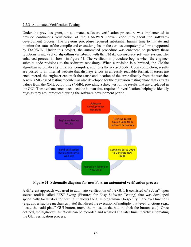
80

7.2.3 Automated Verification Testing

Under the previous grant, an automated software-verification procedure was implemented to provide continuous verification of the DARWIN Fortran code throughout the software-development process. The previous procedure required substantial human time to initiate and monitor the status of the compile and execution jobs on the various computer platforms supported by DARWIN. Under this project, the automated procedure was enhanced to perform these functions using a set of algorithms distributed with the CMake open-source software system. The enhanced process is shown in figure 61. The verification procedure begins when the engineer submits code revisions to the software repository. When a revision is submitted, the CMake algorithm automatically retrieves, compiles, and tests the revised code. Upon completion, results are posted to an internal website that displays errors in an easily readable format. If errors are encountered, the engineer can track the cause and location of the error directly from the website. A new XML-based testing module was also developed for the regression testing phase that extracts values from the XML output file (*.ddb), providing a direct test of the results that are displayed in the GUI. These enhancements reduced the human time required for verification, helping to identify bugs as they are introduced during the software development period.

Figure 61. Schematic diagram for new Fortran automated verification process

A different approach was used to automate verification of the GUI. It consisted of a Java™ open source toolkit called FEST-Swing (Fixtures for Easy Software Testing) that was developed specifically for verification testing. It allows the GUI programmer to specify high-level functions (e.g., add a fracture mechanics plate) that direct the execution of multiple low-level functions (e.g., locate the “add plate” GUI button, move the mouse to the button, click the button, etc.). Once defined, the high-level functions can be recorded and recalled at a later time, thereby automating the GUI verification process.

81

7.3 OEM EVALUATION

The Steering Committee was instrumental in the development of the DARWIN computer program. In addition to providing algorithms and design guidance, the partner companies also participated in substantial code-review efforts to verify the accuracy and usability of the DARWIN software.

7.3.1 Quantitative Verification

DARWIN was evaluated by each of the four PDRI Steering Committee companies throughout the project. The evaluations consisted of a series of studies focused on comparison of DARWIN predictions to experimental data, field experience, and OEM in-house code results. These studies included an extensive set of test cases that were exercised by multiple users within each of the four OEM companies. The studies were performed using DARWIN versions 6.0 through 7.1, primarily on PC computer platforms. OEM evaluation of DARWIN Alpha and Beta versions identified a number of bugs that were fixed prior to the production release of the code and also helped to improve user confidence in the quantitative results.

7.3.2 Qualitative Evaluation

The PDRI Steering Committee performed a series of evaluations to assess the practical use of DARWIN in a design environment. In collaboration with the FAA and the AIA RISC Committee, the Steering Committee identified a number of key enhancements to improve the use of DARWIN as a design and certification tool. Examples include the special analysis mode for certification assessment of titanium HA anomalies for AC 33.14-1, and several capabilities for assessment of hole features outlined in AC 33.70-2, including user specification of manufacturing process credits, an FAA hole feature surface damage report form, and a special analysis mode for certification of hole features. Many additional DARWIN features were improved based on the guidance from the Steering Committee.

7.3.3 OEM Review Comments

Over the course of the PDRI program, the OEMs provided general feedback regarding their experiences with the DARWIN code. The response was very positive, with additional OEMs electing to license DARWIN for certification of new engine rotors and disks. Some OEMs used the deterministic fracture mechanics capability in DARWIN to supplement (or replace) their internal fracture codes.

The OEMs also provided a number of positive comments related to the overall ease of use of DARWIN. Several manufacturers mentioned that the GUI was very easy to understand, and that new users could quickly learn to use it with minimal training. The OEMs also mentioned that the DARWIN User’s Manual was well-documented and provided substantial assistance to both new and experienced users of the code.

82

8. TECHNOLOGY TRANSFER

8.1 PROGRESS REPORTS AND REVIEW MEETINGS

Regular communication with the FAA, the project Steering Committee, and the aircraft engine industry facilitated effective oversight of the research project and timely transfer of important new results. Written reports included brief monthly progress reports and substantially longer interim progress reports, which were issued twice per year to coincide with program review meetings or with major project reports to RISC. One-day program review meetings with the FAA were typically held once per year, with specific schedules directed by the FAA. The project Steering Committee conducted a 1–2 day working meeting in conjunction with each program review meeting. A short status report on program activities was presented at each meeting of the RISC (generally held three times per year). Once per year, the SwRI Program Manager and one of the SwRI co-Principal Investigators attended the RISC meeting in person and made the project presentation. This facilitated additional interaction with the FAA personnel present at the RISC meeting. The Steering Committee often held a working meeting in conjunction with this particular RISC meeting. At other RISC meetings, the SwRI Program Manager typically made the project presentation via a telephone link. Additional face-to-face working meetings were conducted as needed. In addition, the Steering Committee conducted periodic telephone meetings, typically one or two times per month.

8.2 CONFERENCE PRESENTATIONS AND JOURNAL ARTICLES

Important results from this research program were disseminated to a much broader audience in the gas-turbine-engine community or the international technical community in disciplines such as fracture mechanics, or reliability through presentations at conferences and symposia or publications in archival technical journals. A complete listing of these presentations and publications is provided in appendix I.

8.3 DARWIN COMMERCIAL LICENSING

At the request of industry and the FAA, an infrastructure had been developed previously to support the formal use of DARWIN by engine companies for official FAA and company purposes. The DARWIN software was first offered for commercial licensing in 2000. The licensing activity has grown slowly and steadily since that date. DARWIN license fees collected by SwRI are used exclusively to enhance the DARWIN code and to provide user support for the benefit of engine manufacturers, other licensees, and the FAA. No FAA funds from the current project were used to support the licensing activity.

At this writing, a total of ten commercial DARWIN licenses are active, including seven manufacturers of gas turbine engines for aircraft applications, one manufacturer of gas turbine engines for land-based power generation, and two foreign government laboratories. Discussions are continuing with other prospective licensees.

SwRI staff has conducted DARWIN training workshops for specific DARWIN licensee companies by request, with all the costs of presenting the workshop supported by licensing funds. The workshop curriculum was adapted from the curriculum prepared for previous FAA training

83

workshops. Three different workshops for licensee companies were conducted during the term of the current project, and a total of approximately 35 people were trained in these workshops.

In accordance with the terms of the FAA grant agreement, agencies of the U.S. government are entitled to receive a royalty-free license for DARWIN upon request. Licensing to these agencies is described further in section 8.4.

A number of significant enhancements to DARWIN were funded entirely or substantially with licensing revenue. These enhancements include encryption capability for material property data files, two new FCG equations (the NASGRO 4.0 equation and a smoothed multilinear equation), a major GUI redesign to create a deterministic analysis mode, revision of the PC version of DARWIN for compatibility with Windows Vista® and Windows 7, partial funding for development of the FE2NEU translator (including full funding of the translator modulus for ABAQUS), and a host of minor GUI enhancements.

8.4 TECHNOLOGY TRANSFER TO OTHER U.S. GOVERNMENT AGENCIES

DARWIN is available royalty-free to all U.S. government agencies. To date, DARWIN has been distributed to several branches of the Department of Defense, including the Army, Air Force, and Navy. Under the current grant, DARWIN has been distributed for use at the Air Force Research Laboratory (AFRL) (Dayton, OH), the United States Air Force (USAF) Aeronautical Systems Center (ASC) (Dayton, OH), and the Naval Air Systems Command (NAVAIR) (Patuxent River, MD). AFRL is using DARWIN to support their research into fatigue behavior of gas-turbine engine materials. The USAF ASC is investigating the use of DARWIN to supplement remaining life predictions and fleet assessments of aircraft gas-turbine engines in the Air Force. NAVAIR is using DARWIN to assess the influences of inspection and surface treatments on the fatigue lives of aircraft gas-turbine-engine rotating components subjected to fretting and HCF.

SwRI has been collaborating with NASA since 2001 on the development and distribution of the NASGRO analysis software for fracture mechanics and FCG. NASGRO shares some functionality with the Flight_Life fracture mechanics module in DARWIN, and also shares a number of specific SIF solutions. Most of the new or enhanced WF SIF solutions developed under this grant (SC19, SC17, TC15, EC04, and EC05) and the related enhancements to computational efficiency have been implemented in recent versions of NASGRO. As noted earlier, one NASGRO SIF solution (CC11) was implemented in DARWIN. NASGRO is used extensively by NASA, NASA contractors, the European Space Agency, the FAA (especially by FAA Designated Engineering Representatives for damage-tolerance analysis), and many aerospace companies. Industrial NASGRO users in the aircraft, rotorcraft, and gas-turbine-engine businesses include 17 major companies comprising the NASGRO Consortium (Airbus, Alcoa, Boeing, Bombardier, Embraer, Hamilton Sundstrand, Honda [Aircraft Engine R&D Center], Honeywell, Israel Aerospace Industries, Lockheed Martin, Mitsubishi Heavy Industries, Siemens Energy, Sikorsky, SpaceX, Spirit AeroSystems, United Launch Alliance, and Volvo Aero) and more than 300 licensees.

8.5 DARWIN SPINOFF PROJECTS

One of the clearest indications of technology transfer to other government agencies, as well as commercial licensees, is the growing number of independent research projects funded by these

84

other organizations for additional development and implementation of new DARWIN technology that is specifically relevant to their own applications. Although these independent projects have all been modest in size—usually 1 year or less in duration, with limited funding—they have each contributed to the growing capabilities of DARWIN. In most cases, the technology resulting from the project has been implemented in the commercial production version of DARWIN or published, and therefore is available to all DARWIN users.

For convenience, the following sub-sections provide thumbnail sketches of many of these projects. A few projects conducted for individual commercial licensees were proprietary in nature and, therefore, are not mentioned here.

8.5.1 Enhanced Life-Prediction Technology for Engine Rotor Life Extension

AFRL funded this multi-year Dual-Use Science and Technology (DUS&T) project at SwRI to support their Engine Rotor Life Extension (ERLE) program. The ERLE goal is to extend the life of certain life-limiting components, without increasing risk, by systematically improving, and more effectively integrating a number of life-management technologies—life prediction, nondestructive inspection, engine-health monitoring, maintenance, and repair. The project developed physics-based, deterministic, probabilistic, fatigue-life prediction models that support the objectives of ERLE and the broader goals of Condition Based Maintenance Plus (CBM+). The new models incorporated small-crack effects and enabled enhanced fracture mechanics analysis of high-stress gradients associated with residual, contact, and thermal stresses. The importance of uncertainty in mission usage was highlighted, and a statistical method to automatically identify mission type from usage data was introduced. Probabilistic simulations incorporating input from an embedded sensor model were used to demonstrate the effectiveness of engine-health monitoring. Mature technology from the program was incorporated into DARWIN to facilitate technology transfer to AFRL and the turbine-engine community. These DARWIN enhancements included a special model for total fatigue life prediction at severe stress gradients, facilities for superimposing local residual stress fields with service stresses for SC SIF solutions, and facilities for specifying changes to the mission mix as a function of flight cycles. Additional details are available elsewhere [30].

8.5.2 Extension of Bimodal Failure Distribution Concepts

Previous research at AFRL observed that the variability in fatigue lifetimes for laboratory smooth specimens can sometimes be attributed to multiple crack formation mechanisms. A proper probabilistic treatment of this bimodal distribution should provide a more accurate description of lower-bound lifetimes that could be used in design, eliminating the over-conservatism that may occur if both populations are lumped together into a single distribution. The objective of this one-year AFRL-funded project was to build on the strong foundation established at AFRL and develop a more rigorous probabilistic framework for fatigue life prediction when multiple failure mechanisms are operative. This new framework is needed to facilitate application of the predictive schemes to practical component geometries that exhibit a variety of sizes, shapes, and stress distributions. Deterministic and probabilistic life models were developed for crack formation and crack growth in IN-100 at two anomaly types and two locations for four stress levels. These probabilistic life models were combined with anomaly occurrence rates using a series system model to predict lifetime behavior in laboratory coupons using DARWIN. The predictions showed

85

general agreement with observed laboratory coupon behavior. The model provided a rigorous basis to explore fatigue life behavior in alternative specimen sizes. Further details are available elsewhere [31].

8.5.3 Integrated Processing and Probabilistic Lifing Models for Superalloy Turbine Disks

Integrated Computational Materials Engineering aims to merge the computational simulation of materials, manufacturing processes, and component design into a holistic system to optimize components before they are fabricated. AFRL is funding efforts to link computational simulations of manufacturing processes with probabilistic damage-tolerance analysis. DARWIN is being linked with the manufacturing process software tool DEFORM, developed by Scientific Forming Technologies Corporation (SFTC), which can simulate rotor manufacturing processes, including forging, heat treating, and machining.

In an exploratory 9-month Phase I Small Business Innovative Research (SBIR) project conducted jointly by SwRI and SFTC, an initial link was established to transfer DEFORM calculations of location-specific bulk residual stresses that emerge in the rotor during manufacturing into DARWIN, and then use this information in DARWIN to inform FCG life computations. The effect of the manufacturing residual stresses on life and risk results was demonstrated for an idealized rotor geometry.

Based on the success of the Phase I feasibility study, AFRL has awarded SFTC and SwRI a larger two-year Phase II project to extend this DEFORM-DARWIN linkage to address both microstructure (location-specific average grain size) and anomaly characterization (location-specific anomaly orientation), and also to extend the linkage from deterministic descriptions to parametric and probabilistic descriptions of the relevant variables.

8.5.4 Three-Dimensional Crack Growth Life Prediction for Probabilistic Risk Analysis of Turbine Engine Metallic Components

This AFRL-funded effort developed and evaluated a prototype interface between DARWIN and FRANC3D, an existing high-fidelity FE crack growth simulator. The effort was based on the capability to link DARWIN with SIF solutions generated outside of DARWIN through user-provided tables, a capability developed in the current grant and described earlier in section 3.3. The main technical objective was to demonstrate that uncertainty and conservatism in probabilistic life predictions could be reduced by using high-fidelity models for three-dimensional crack growth.

In an exploratory 9-month Phase I SBIR project conducted jointly by SwRI and Fracture Analysis Consultants (FAC), the developer of FRANC3D, DARWIN was modified to write a script for FRANC3D indicating the size, location, and orientation of an initial crack in an ANSYS or ABAQUS FEM. FRANC3D then inserted the crack into the FEM and generated a table of SIF versus crack size as the crack grew, ultimately returning this table back to DARWIN to perform FCG lifetime and probabilistic risk assessments. The prototype interface was verified by performing comparative calculations on two simple geometries for which DARWIN already had built-in WF SIF solutions. Next, the system was applied to a complex integrally bladed rotor (IBR) model for which existing DARWIN SIF solutions were inadequate. The differences in calculated

86

FCG lifetime and probability of fracture for the IBR model demonstrated the potential benefits of the new integrated tool.

Based on the success of the Phase I feasibility study, a larger 2-year SBIR Phase II project has recently been awarded by AFRL to FAC and SwRI for further development and evaluation of the integrated tool.

8.5.5 Probabilistic Fretting Fatigue Assessment of Gas Turbine Engine Disks

The objective of this study (funded by NAVAIR over a 4-year period and performed by SwRI and AFRL) was to assess the influences of inspection and surface treatments on the fatigue lives of aircraft gas-turbine-engine rotating disks subjected to fretting and HCF load effects. This study involved calculation of the stress field in the disk/blade interface of a typical gas-turbine-engine disk using available contact mechanics models, estimation of fretting fatigue life, and probabilistic risk assessment using DARWIN. Contact stresses were calculated using the numerical solution of the singular integral equation that characterizes the contact interface that was applied to the stress results of a FEA model of a gas-turbine-engine blade and disk. Both the CAPRI (Contact Analysis for Profiles of Random Indentors) software and the Worst Case Fret techniques were used for this computation. Fatigue lives and fracture risks were computed using DARWIN. The influences of residual stresses associated with surface treatments and nondestructive inspections were also assessed via DARWIN. The influences of high-cycle fatigue load effects were also considered, first by considering the HCF threshold model in DARWIN and then by modeling the LCF and HCF stresses as separate input variables. The results from this study indicated that surface treatments and scheduled depot inspections had the potential to significantly reduce the probability of fracture associated with fretting fatigue. In addition, it was shown that although HCF stress effects could initiate and propagate small cracks, they could not propagate cracks beyond the contact region of the disk because of the steep gradient in this region. It was shown that HCF stresses were sufficiently large enough to cause blade failures, which was confirmed by NAVAIR field experience.

8.5.6 Probabilistic Mission Analysis for Assessment of Alternative Fuels in Turbine Engines

The objective of this study funded by NAVAIR over a 1-year period and performed by SwRI was to develop a probabilistic mission analysis capability that could ultimately be used for assessment of alternative fuels in turbine engines. Under the recently completed first phase of this project, previously developed algorithms for the nonparametric estimation of engine usages were enhanced and applied to engine RPM data from actual usage histories provided by NAVAIR to develop probabilistic forecasting models of future engine usage for aircraft engine applications. Under the second phase, currently underway, fatigue life and associated fracture risk will be assessed using DARWIN for various aircraft engine fleets based on the usage data provided by NAVAIR.

8.5.7 Life and Reliability Prediction for Turbopropulsion Systems

The objective of this 6-month NAVAIR-funded SBIR Phase I project, performed by Mustard Seed Software and SwRI, was to develop an innovative methodology for life and reliability prediction of hot-section components in advanced turbopropulsion systems. The project focused on addressing the effects of competing time-dependent damage modes, including creep, stress

87

corrosion, and stress rupture on long-term performance and reliability of engine disks made from Ni-based superalloys that could exhibit location-specific microstructures, microstructural variability, or evolution of microstructures after thermal exposures at elevated temperatures for extended time periods. Building on the time-dependent crack-growth framework developed for the current FAA project, a set of three generic time-dependent crack growth models was implemented and integrated into DARWIN, along with GUI enhancements to facilitate entry of material property data and time-dependent mission information. A framework was developed for extending the Phase I methodology to treat crack-growth variability due to microstructural variation using the MicroFaVa probabilistic micromechanics software [32] with a plan for future work and transition to industry.

8.5.8 Lifing Technology for Powder Metallurgy Alloys

NASA Glenn Research Center (GRC) has been independently investigating probabilistic lifing methods for gas turbine rotor materials for many years. GRC funded a 1-year project at SwRI to investigate this technology with a view toward a future integration of GRC methods/models for powder metallurgy nickel rotor alloys into DARWIN. The current status of GRC data and models and the DARWIN software was reviewed, and significant accomplishments, capabilities, and technology gaps were identified. New algorithm development was conducted in three areas. First, a method to estimate anomaly distributions for materials with multiple anomaly types was developed and verified, building on earlier SwRI work for AFRL. Second, an unfolding algorithm to estimate the dimensions and orientations of 3D spheroids based on 2D sectioning measurements was implemented and investigated. Third, the behavior of small fatigue cracks in U720 tests was investigated, and an existing model to predict small-crack behavior was evaluated in conjunction with similar studies of other rotor materials in the current FAA project. Finally, a program plan was outlined for future research, identifying the most significant opportunities to address technology gaps and to develop new DARWIN capabilities. Additional details are available elsewhere [33].

8.5.9 Hot Corrosion of Nickel-Based Turbine Disks

Anticipated increases in turbine inlet temperatures will increase the likelihood of Type II corrosion damage, which is typically characterized by localized corrosion pitting caused by melting of sulfur-containing salts. These Type II hot corrosion pits have been shown to decrease the fatigue resistance of superalloys due to initiation of fatigue cracks at hot corrosion pits. However, the rigorous analytical models and tools needed by turbine engine designers to predict Type II corrosion effects are not currently available. Barron Associates and SwRI were awarded a 9-month SBIR Phase I project to investigate the feasibility of integrating probabilistic models for these effects into DARWIN. The key Phase I innovations included enhanced probabilistic models that are explicitly parameterized by the relevant environmental and material variables. The models are a significant step toward modeling the spatial and temporal evolutions of corrosion pits, setting the stage for the development of fatigue life prediction capability. Based on these preliminary results, the team has also been awarded a 2-year Phase II project, with an ultimate objective of creating a functional prototype of DARWIN that includes Type II hot corrosion effects.

88

8.5.10 Extension of DARWIN for Continued Airworthiness Assessment

In 1991, the AIA created the Continued Airworthiness Assessment Methodologies (CAAM) Committee to develop methods to resolve safety-related problems associated with engines and auxiliary power units installed on transport aircraft. The CAAM Committee developed FAA AC 39-8, which describes a process for characterizing and assessing the risk associated with safety-related events. It specifies per-flight target risk values (risk factors) associated with so-called short-term and long-term risk. It also describes a procedure for computing the risk of safety-related events using Monte Carlo simulation that is similar to the approach that is used in DARWIN to predict the risk of fracture of rotating components. However, AC 39-8 requires a risk assessment of an entire fleet of aircraft that could consist of different types of aircraft and usages, whereas DARWIN was designed to assess the risk associated with a single usage.

In 2006, MTU funded SwRI to develop a fleet-assessment capability to enable the combination of risk results from individual DARWIN runs for engines with different usages and aircraft configurations to aid in the assessment of fleet risk outlined in AC 39-8. The fleet assessment capability is a separate module that is executed from the DARWIN GUI that enables the user to select DARWIN results files and to view the combined risk results over the lifetime of the entire fleet. A capability is included that enables the user to specify the timing that each engine is placed into service for this assessment.

9. SUMMARY

Major accomplishments of the “Probabilistic Design for Rotor Integrity” research grant are summarized in the following paragraphs:

New DARWIN versions 6.0, 6.1, 7.0, 7.1, and 7.2 were released to the FAA and industry. Each new version was evaluated thoroughly by the development team, the project steering committee, and RISC before being released for production use. Specific enhancements are described below. 

DARWIN was enhanced to improve its use for certification assessments associated with FAA ACs. Special analysis modes were implemented for titanium HA anomalies as addressed in AC 33.14-1 and hole features as addressed in AC 33.70-2. DARWIN was further enhanced to support assessment of hole features, including user specification of manufacturing process credits and an FAA report form.

Ten commercial DARWIN licenses are currently active, including seven manufacturers of gas turbine engines for aircraft applications. Licensing revenue was used to fund additional enhancements to DARWIN and training workshops for licensees.

The expanding capabilities of DARWIN, its increasing use in industry, and growing interest in DARWIN among other agencies have all contributed to a significant number of DARWIN spinoff projects funded by AFRL, NAVAIR, NASA, and individual DARWIN users. These projects typically result in significant new capabilities in the main DARWIN software delivered to the FAA and all other DARWIN users. 

Superposition models for crack growth as an independent sum of cycle-dependent and time-dependent terms were derived and implemented in DARWIN. Crack growth experiments were performed on fine-grained IN-718 surface-crack tension specimens at

89

different elevated temperatures with and without dwell periods to demonstrate the suitability of this model to predict time-dependent crack growth in rotor materials.

Additional time-dependent crack growth experiments performed on different specimen geometries and at different stress ratios with another fine-grained IN-718 indicated some possible limitations of conventional superposition methods. An alternative analysis method employing an equivalent SIF that attempts to characterize the effects of local constraint on the crack tip was proposed, but has not yet been fully developed or validated.

Modified Willenborg models for overload retardation effects in both cyclic and dwell crack growth were implemented in DARWIN. A series of IN-718 crack-growth tests were performed to demonstrate the retardation effect and to evaluate the models.

Several advanced models for predicting FCG rates under non-isothermal conditions using only FCG properties derived from isothermal testing were identified and implemented in DARWIN. Each model has been used successfully by at least one of the steering committee companies in their own internal methods for some applications, but further work is needed to establish the general applicability (or any limitations) of each method.

An exploratory experimental and analytical study was conducted on the effects of time-dependent shakedown at stress concentrations during hot compression cycles on the resulting FCG rate. These effects were found to be potentially significant and a simple model was developed to address them.

A literature survey of small-crack effects in a variety of common gas turbine engine rotor materials was performed. A simple engineering model for small-crack behavior was critically evaluated, and the practical significance of small-crack effects for life prediction in rotor applications was evaluated. Because no small-crack data were found in the literature for the common rotor material IN-718, an experimental procedure was developed to generate growth rate data for small fatigue cracks in this alloy.

A limited experimental investigation was conducted to characterize the impact of naturally occurring material anomalies on the fatigue performance of rotor grade conventional nickel material—specifically, double melted IN-718. Material that appeared to contain significant anomalies had previously been identified; forged and heat treated to rotor specification; and inspected. Fatigue specimens containing embedded anomalies were machined and tested. Two successful tests indicated that a significant fraction of the total fatigue life was associated with crack formation at a known anomaly.

FCG data were generated with different specimen geometries for a fine-grained delta-processed IN-718 alloy to facilitate the validation of DARWIN SIF solutions and related FCG algorithms. Analysis results confirmed the suitability of DARWIN methods for the geometries considered, although experimental scatter complicated one assessment.

A new bivariant WF SIF solution (SC19) was developed for an offset semi-elliptical SC, verified, and implemented in DARWIN. Based on this work, the geometry limits for the corresponding univariant solution (SC17) were also increased.

Several enhancements were derived and implemented to significantly improve the computational efficiency of DARWIN SIF solutions. Bivariant solutions were improved by replacing the customary double integration by a simple double summation based on tabular WF values and interpolated nodal stress. Selected univariant SIF solutions were improved by approximating the stress variation between user-specified stress values by Hermite polynomials and then replacing the customary integration with one single pass of simple summation so that no further numerical iteration is required.

90

An approximate SIF solution was developed for a through-thickness edge crack in a variable thickness plate, verified, and implemented in DARWIN. The solution requires the thickness variation to be modeled as symmetrical to the mid-plane of the plate. The corresponding DARWIN GUI allows the user to specify a piecewise linear thickness variation in the model, based on interrogation of the underlying FEM, and to immediately visualize the resulting fracture model.

New bivariant (EC04) and univariant (EC05) WF SIF solutions for an offset elliptical embedded crack in plate were developed, validated, and implemented in DARWIN.

The existing bivariant WF SIF solution CC09 for a quarter-elliptical corner crack in a plate was enhanced to permit use for corner angles that deviated 5 from 90.

A new univariant WF SIF solution for a corner crack in a plate (CC11) was implemented in DARWIN. This solution was developed previously by SwRI under NASA funding.

A new shakedown module for bivariant stressing was developed and implemented in DARWIN. This methodology is for proportional loading and is applicable to 2D rectangular load-bearing sections whose elastic stress results are available and provided by the user as input. The methodology converts the linear-elastic solution into an elastic-plastic solution while conserving forces and moments.

A new capability was implemented that allows importing an externally generated table of SIF values into DARWIN for use in life and fracture risk computations. The crack size is characterized by a single-length parameter with a definition established by the user.

An alternative stress-ratio model for fatigue cycles containing nominally negative (compressive) stresses was derived and implemented in DARWIN. The alternative model is particularly needed to use SIF values generated by FE simulations of growing cracks because the conventional definition of stress ratio may not be meaningful when a compressive stress is applied to the model and the crack itself is closed.

A new capability was implemented in DARWIN that allows the user to include the influence of vibratory HCF stress values in FCG and fracture risk computations. Fracture is conservatively assumed to occur when the SIF range associated with the HCF stress alone exceeds the FCG threshold value.

An algorithm was developed and implemented in DARWIN to predict the number of flight cycles associated with a user-specified probability of fracture (target risk) value.

A DARWIN capability to address stress concentration factor gradients in 2D axisymmetric models was developed to support inherent anomaly assessments. The capability was extended to provide treatment for stress concentrations at turned surfaces.

A new surface-zoning capability for 2D axisymmetric FE models was implemented in DARWIN to provide support for risk assessment of turned surfaces. A new capability to characterize surface area at blade slots was also developed to support RISC activities.

Automated modeling capabilities were implemented in DARWIN to reduce the cost and the human-factors variability in the current analysis process. These capabilities include automatic construction of fracture mechanics models (autoplate), life contours, and autozoning. The autoplate algorithm determines the initial crack type and the orientation and size of an idealized fracture mechanics plate model for 2D FEM geometry and stress results. Autoplate can be used to construct life contours based on initial cracks placed at each of the nodes in a FEM. Risk contours are developed in a similar fashion to life contours, except that a distribution of initial crack sizes is applied at each FE. The process of automated risk contour creation is also referred to as autozoning.

91

The FE2NEU FE results translator was developed to convert ANSYS and ABAQUS FE results to the neutral file format required by DARWIN. The new translator supports all the FE types and filtering capabilities in the previous ANS2NEU translator. New capabilities include support for newer ANSYS versions and large results files, improved computational efficiency, filtering by ANSYS Named Components, and reduced maintenance costs. Supplementary funds for this development were provided by DARWIN licensing revenue.

A new parallel-processing capability was implemented in DARWIN that automatically distributes the risk-assessment code computations to multiple processors on a single computer using the OpenMP approach. The process requires no additional intervention from the user. Testing confirmed substantial reductions in computation time.

A number of other enhancements to DARWIN computational efficiency and accuracy were developed and implemented. These include an enhanced restart algorithm, an alternative treatment of shakedown with stress scatter, a new FCG life interpolation algorithm, an enhanced mesh-generation algorithm for onion skins, a new method for critical anomaly size calculation, a new algorithm for the LAF method, and new software compilation protocols.

Several stress-processing enhancements were developed and implemented in DARWIN to support new features and to improve the computational efficiency of existing capabilities. New algorithms were developed to improve the efficiency of identifying stress values within large FEMs. Other enhancements provide support for multiple load steps in 3D FEMs and load-step scaling factors.

A number of database and file management enhancements were performed to address the increasing amount of data associated with DARWIN assessments. The DARWIN input and output files were converted to an XML format for improved efficiency and error reduction, and verbosity controls were introduced to enable the user to control the amount of data printed to output files. Additional optional deterministic fracture output was provided for verification purposes. Other enhancements enable the user to filter the display of warning messages and to view the list of optional features for a GUI session.

Several significant enhancements were implemented to DARWIN internal verification procedures. These included verification of individual modules prior to integrating them into the main source code, incremental releases of alpha versions, and automated verification whenever a code developer uploads new source code into the DARWIN repository. These improvements resulted in a substantial reduction in the number of bugs in code releases as well as the time and cost associated with the code-maintenance effort.

10. REFERENCES

1. FAA Report. (2000). Turbine Rotor Material Design. (DOT/FAA/AR-00/64).

2. McClung, R.C., Lawless, B.H., Gorelik, M., Date, C., Gill, Y., and Piascik, R.S. (1999) Fatigue Crack Growth of Titanium Rotor Alloys in Vacuum And Air. In R.R. Boyer, D. Eylon, and G. Lutjering (Eds.), Fatigue Behavior of Titanium Alloys, (211–218). Pittsburgh, PA: The Minerals, Metals, and Materials Society.

3. Chan, K.S., Perocchi, L., and Leverant, G.R. (2000). Constitutive Properties of Hard Alpha Titanium. Metallurgical and Materials Transactions A, 31(12), 3029–3040.

92

4. Chan, K.S. (2001). Constitutive Relations for Inelastic Deformation and Damage Accumulation in Hard Alpha Titanium. ASME Transactions, Journal of Engineering Materials and Technology, 123(3), 281–286.

5. McKeighan, P.C., Perocchi, L.C., Nicholls, A.E., and McClung, R.C. (1999). Characterizing the Cracking Behavior of Hard Alpha Defects in Rotor Grade Ti-6-4 Alloy. Fatigue Behavior of Titanium Alloys, (349–356) Pittsburgh, PA: The Minerals, Metals, and Materials Society.

6. Wu, Y.-T., Enright, M. P., and Millwater, H.R. (2002). Probabilistic Methods for Design Assessment of Reliability with Inspection. AIAA Journal, 40(5), 937–946.

7. Millwater, H., Wu, J., Riha, D., Enright, M., Leverant, G., McClung, C., Kuhlman, C., et al. (2000). A Probabilistically-based Damage Tolerance Analysis Computer Program for Hard Alpha Anomalies in Titanium Rotors. Paper 2000-GT-0421. Proceedings from the 45th ASME International Gas Turbine & Aeroengine Technical Congress, Munich, Germany.

8. FAA Report. (2008). Turbine Rotor Material Design—Phase II. (DOT/ FAA/AR-07/13).

9. Laz, P.J., Chan, K.S., McClung, R.C., and Leverant G.R. (2003). Effects of CTE-Induced Residual Stresses Around Hard Alpha Particles on Fatigue Crack Growth in Ti-6Al-4V. Fatigue and Fracture of Engineering Materials and Structures, 26(12). 1145–1157.

10. McClung, R.C., Enright, M.P., Lee, Y.-D., Huyse, L., and Fitch, S. (2004). Efficient Fracture Design for Complex Turbine Engine Components. Paper GT-2004-53323. Proceedings from the 49th ASME International Gas Turbine & Aeroengine Technical Congress, Vienna, Austria.

11. Enright, M.P., Lee, Y.-D., McClung, R.C., Huyse, L., Leverant, G.R., Millwater, H.R., and Fitch, S.K. (2003). Probabilistic Surface Damage Tolerance Assessment Of Aircraft Turbine Rotors. Paper GT-2003-38731. Proceedings from the 48th ASME International Gas Turbine & Aeroengine Technical Congress, Atlanta, Georgia.

12. Lee, Y.-D., R.C. McClung and Chell, G.G. (2008). An Efficient Stress Intensity Factor Solution Scheme for Corner Cracks at Holes under Bivariant Stressing. Fatigue and Fracture of Engineering Materials and Structures, 31(11). 1004–1016.

13. McClung, R.C. (2007). A Literature Survey on the Stability and Significance of Residual Stresses During Fatigue. Fatigue and Fracture of Engineering Materials and Structures, 30(3). 173–205.

14. Wu, Y.-T., Enright, M.P. and Millwater, H.R. (2000). Efficient and Accurate Methods for Probabilistic Analysis of Titanium Rotors. Paper PMC2000-221 Proceedings from the 8th ASCE Joint Specialty Conference on Probabilistic Mechanics and Structural Reliability, Notre Dame, IN.

93

15. Huyse, L., and Enright, M.P. (2003). Efficient Statistical Analysis of Failure Risk in Engine Rotor Disks Using Importance Sampling Techniques. Paper 2003-1838. Proceedings from the 44th Structures, Structural Dynamics, and Materials Conference, Norfolk, VA.

16. Enright, M.P., and Millwater, H.R. (2002). Optimal Sampling Techniques for Zone-Based Probabilistic Fatigue Life Prediction. AIAA Paper 2002-1383. Proceedings from the 43rd Structures, Structural Dynamics, and Materials Conference, Denver, CO.

17. Enright, M.P., Millwater, H.R., and Huyse, L. (2006). Adaptive Optimal Sampling Methodology for Reliability Prediction of Series Systems. AIAA Journal, 44(3) 523–528.

18. Wei, R.P. and Landes, J.D. (1969). Correlation Between Sustained Load and Fatigue Crack Growth in High Strength Steels. Materials Research & Standards, 9(7) 25–46.

19. Solomon H.D. and Coffin, L.F. (1973). Effects of Frequency and Environment on Fatigue Crack Growth in A286 at 1100F. Fatigue at Elevated Temperatures, ASTM STP 520 (112–124). Philadelphia, PA: American Society for Testing and Materials.

20. Air Force Report. (1988). Advanced Cumulative Damage Modeling. (AFWAL-TR-88-4146).

21. Van Stone, R.H. (1990). Elevated Temperature Crack Growth: Comparison of Interpolation and Superposition Models to Predict Time-Dependent Crack Growth in René 95. Paper presented at the Winter Annual Meeting of the American Society of Mechanical Engineers, Dallas, TX.

22. Van Stone, R.H., and Slavik, D.C. (2000). Prediction of Time-Dependent Crack Growth with Retardation Effects in Nickel Base Alloys. Fatigue and Fracture Mechanics, 31st Volume, ASTM STP 1389. (405–426). West Conshohocken, PA: American Society for Testing and Materials.

23. McClung, R.C., Chan, K.S., Hudak, S.H., Jr., and Davidson, D.L. (1996). Behavior of Small Fatigue Cracks. ASM Handbook, Vol. 19: Fatigue and Fracture, (153–158). Novelty, OH: ASM International.

24. El Haddad, M.H., Smith, K.N., and Topper, T.H. (1979). Fatigue Crack Propagation of Short Cracks. Journal of Engineering Materials and Technology, Transactions of the ASME, 101(1) 42–46.

25. Li, S., Mear, M.E., and Xiao, L. (1998). Symmetric Weak-Form Integral Equation Method for Three-Dimensional Fracture Analysis. Computer Methods in Applied Mechanics and Engineering. 151(3–4), 435–539.

26. Shen, G. and Glinka, G. (1991). Weight Functions for a Surface Semi-Elliptical Crack in a Finite Thickness Plate. Theoretical and Applied Fracture Mechanics, 15(3), 247–255.

27. Lee, Y.-D., Chell, G.G., and Hudak, Jr., S.J. (2003). An Efficient Three-Dimensional Elastic-Plastic Stress Analysis Method for Stress Concentration Features in Isotropic and

94

Anisotropic Materials. Presented at the 8th National Turbine Engine High Cycle Fatigue Conference, Monterey, CA.

28. Emery, J.M., Hochhalter, J.D., Wawrzynek, P.A., Heber, G., and Ingraffea, A.R. (2009). DDSim: A Hierarchical, Probabilistic, Multiscale Damage and Durability Simulation System – Part I: Methodology and Level I. Engineering Fracture Mechanics, 76(10) 1500–1530.

29. L’Ecuyer, P., Simard, R., Chen, J., and Kelton, W. (2002). An Object-Oriented Random-Number Package with Many Long Streams and Substreams. Operations Research, 50(6), 1073–1075.

31. Enright, M.P. and McClung, R.C. (2010). A Probabilistic Framework for Gas Turbine Engine Materials with Multiple Types of Anomalies. Paper GT2010-23618. Presented at the 55th ASME International Gas Turbine & Aeroengine Technical Congress, Glasgow, Scotland.

30. Air Force Report. (2008). Enhanced Life Prediction Technology for Engine Rotor Life Extension (ERLE). (AFRL-RX-WP-TR-2008-4287).

32. Chan, K.S., and Enright, M.P. (2006). A Probabilistic Micromechanical Code for Predicting Fatigue Life Variability: Model Development and Application. ASME Transactions, Journal of Engineering for Gas Turbines and Power, 128(4), 889–895.

33. NASA Report. (2011). Integration of NASA-Developed Lifing Technology for PM Alloys into DARWIN, (NASA/CR—2011-216977).

A-1

APPENDIX A—TIME-DEPENDENT AND OVERPEAK RETARDATION CRACK-GROWTH BEHAVIOR

A.1 PROGRAM OBJECTIVES

The objective of this program was to generate time-dependent crack-growth data and overpeak (OP) crack-growth retardation data for a fine-grained Alloy 718 forging at conditions relevant to gas turbine applications to validate previously proposed models for linear superposition of cyclic and static crack-growth rates and modified Willenborg retardation models for both cyclic and time-dependent crack growth [A-1].

A.2 EXPERIMENTAL BACKGROUND

The program was organized into two parts. The first part focused on crack-growth tests with a range of hold times and a significant fraction of time-dependent crack growth. The second part focused on retardation crack-growth tests with significant amounts of either cyclic or static OP retardation. All of these tests were performed at GE Aviation (GEA).

Test specimens were machined from two fine-grained Alloy 718 forged disks. Both disks were in the solution + age heat treat condition. The microstructure and measured grain size for each of the two forgings is shown in figure A-1 below.

Crack growth data were generated using the Kb bar specimen geometry, which is shown in figure A-2. For tests where a cyclic waveform was used (the continuous cycling tests and the multiple [“mission”] OP tests), the thickness and width of the gauge section was 0.168 inch and 0.40 inch, respectively. This specimen is known as the small surface crack (SC) specimen. For both the hold time tests and the single OP tests, the thickness and width of the gauge section was 0.25 inch and 0.60 inch, respectively. This specimen is known as the large SC specimen.

A semi-elliptical fatigue pre-crack was generated from a 5 × 10 mil electro-discharged machined (EDM) starter notch that was placed in one of the wide faces of the specimen. The specimen was then heat tinted to document the pre-crack size. For all tests in this program, the loading mode was axial. Fatigue crack-growth monitoring was performed using an automated DC electrical potential drop method [A-2]. For all tests, the fatigue crack aspect ratio history was documented using periodic heat tinting.

A-2

Figure A-1. Microstructure of fine grain 718 forgings

Figure A-2. Schematic of Kb BAR test specimen geometry

Alloy 718 Forgings (Solution + Age)

Forging #SN1014

ASTM GS 11

Forging #A30856

ASTM GS 10

Alloy 718 Forgings (Solution + Age)

Forging #SN1014

ASTM GS 11

Forging #A30856

ASTM GS 10

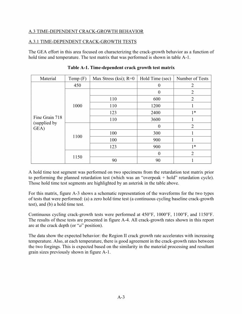
A-3

A.3 TIME-DEPENDENT CRACK-GROWTH BEHAVIOR

A.3.1 TIME-DEPENDENT CRACK-GROWTH TESTS

The GEA effort in this area focused on characterizing the crack-growth behavior as a function of hold time and temperature. The test matrix that was performed is shown in table A-1.

Table A-1. Time-dependent crack growth test matrix

Material Temp (F) Max Stress (ksi); R=0 Hold Time (sec) Number of Tests

Fine Grain 718 (supplied by GEA)

450 0 2

1000

0 2

110 600 2

110 1200 1

123 2400 1*

110 3600 1

1100

0 2

100 300 1

100 900 1

123 900 1*

1150 0 2

90 90 1 A hold time test segment was performed on two specimens from the retardation test matrix prior to performing the planned retardation test (which was an “overpeak + hold” retardation cycle). Those hold time test segments are highlighted by an asterisk in the table above.

For this matrix, figure A-3 shows a schematic representation of the waveforms for the two types of tests that were performed: (a) a zero hold time test (a continuous cycling baseline crack-growth test), and (b) a hold time test.

Continuous cycling crack-growth tests were performed at 450°F, 1000°F, 1100°F, and 1150°F. The results of these tests are presented in figure A-4. All crack-growth rates shown in this report are at the crack depth (or “a” position).

The data show the expected behavior: the Region II crack growth rate accelerates with increasing temperature. Also, at each temperature, there is good agreement in the crack-growth rates between the two forgings. This is expected based on the similarity in the material processing and resultant grain sizes previously shown in figure A-1.

A-4

(a) (b)

Figure A-3. Schematic representations of (a) Continuous cycling waveform, and (b) Hold time waveform

Figure A-4. Continuous cycling (20 CPM) data

The continuous-cycling (20 CPM) data and the hold-time data at 1000°F are plotted on a da/dN (crack growth per cycle) basis in figure A-5. The data show the expected behavior: the crack growth rates systematically increase with increasing hold time. Note the excellent agreement between the two 600-second hold time tests (one from each forging).

The 1100°F 20 CPM data and the 1100°F hold time data are plotted on a da/dN basis in figure A-6. The data again show the expected behavior: the crack growth rates systematically increase with increasing hold time. Note that duplicate 1100°F tests from a single forging (with 900-second hold time) show excellent agreement.

Alloy 718 Continuous Cycling (Baseline)

Time (seconds)

Str

ess

(ksi

)Alloy 718 Hold Time Cycle

Time (seconds)

Str

ess

(ksi

)

One cycle Repeats

1.00E-07

1.00E-06

1.00E-05

1.00E-04

10 100

del K - ksi*sqrt(in)

da/

dN

- i

n/c

ycle SN1014-1, 450F

A30856-25, 450F

SN1014-5, 1000F

A30856-26, 1000F

SN1014-2, 1100F

A30856-27, 1100F

SN1014-6, 1150F

A30856-28, 1150F

A-5

Figure A-5. Continuous cycling (20 CPM) and hold time data at 1000°F

Figure A-6. Continuous cycling (20 CPM) and hold time data at 1100°F

The same da/dN comparison (20 CPM and hold-time data) for 1150°F is shown in figure A-7. Again, the data show the expected behavior, with the 90-second hold-time crack-growth rate greater than the continuous cycling crack-growth rate.

1.00E-06

1.00E-05

1.00E-04

1.00E-03

1.00E-02

10 100

del K - ksi*sqrt(in)

da/

dN

- i

n/c

ycle

A30856-26, 20 cpm

SN1014-5, 20 cpm

A30856-18, 600 sec

SN1014L-1, 600 sec

SN1014L-6, 1200 sec

A30856-25, 2400 sec hold

A30856-19, 3600 sec hold

1.00E-06

1.00E-05

1.00E-04

1.00E-03

1.00E-02

10 100

del K - ksi*sqrt(in)

da

/dN

- i

n/c

yc

le A30856-27, 20 cpm

SN1014-2, 20 cpm

A30856-20, 300 sec

SN1014L-7, 900 sec

SN1014-12, 900 sec

A-6

Figure A-7. Continuous cycling (20 CPM) and hold-time data at 1150°F

A.3.2 TIME-DEPENDENT CRACK GROWTH MODELING

At each temperature, the time-dependent crack growth data were successfully modeled using the linear superposition model of cyclic and static crack growth rates [A-1]:

(A-1)

In this relationship, da/dN is based on K, whereas da/dt is based on Kmax. For the R = 0 test cycle evaluated in this program, K = Kmax. The static crack growth rates (da/dt) were plotted as a function of Kmax in figures A-8, A-9, and A-10 for 1000°F, 1100°F, and 1150°F, respectively.

The static crack-growth rates at 1100°F (Figure A-9) showed little variation. However, the 1000°F, 3600-second hold time test (figure A-8) was approximately two times faster than the remainder of the 1000°F tests at higher Kmax values. It is important to realize that the static crack-growth rates at 1000°F are approximately an order of magnitude slower than at 1100°F and that, in general, the 1000°F tests have a lower contribution of time-dependent crack growth. This makes the experimental determination of static crack growth rates more difficult. The variation of the 1000°F test data will be evaluated more fully later in the report.

1.00E-06

1.00E-05

1.00E-04

1.00E-03

1.00E-02

10 100

delK - ksi*sqrt(in)

da/

dN

- in

/cyc

le

1014L-8, 90 sec

SN1014-6, 20 cpm

A30856-28, 20 cpm

holdtdtdadNdacycletimeholddNda //)(/

A-7

Figure A-8. 1000°F time-dependent data plotted as Kmax vs. Da/Dt

Figure A-9. 1100°F time-dependent data plotted as Kmax vs. Da/Dt

1.00E-08

1.00E-07

1.00E-06

1.00E-05

1.00E-04

10 100

Kmax - ksi*sqrt(in)

da/

dT

- in

/sec

A30856-18, 600 sec

SN1014L-1, 600 sec

SN1014L-6, 1200 sec

A30856-25, 2400 sec hold

A30856-19, 3600 sec hold

Regression fit

1.00E-08

1.00E-07

1.00E-06

1.00E-05

1.00E-04

10 100

Kmax - ksi*sqrt(in)

da/

dT

- in

/sec A308856-20, 300 sec

SN1014L-7, 900 sec

SN1014L-12, 900 sec

Regression fit

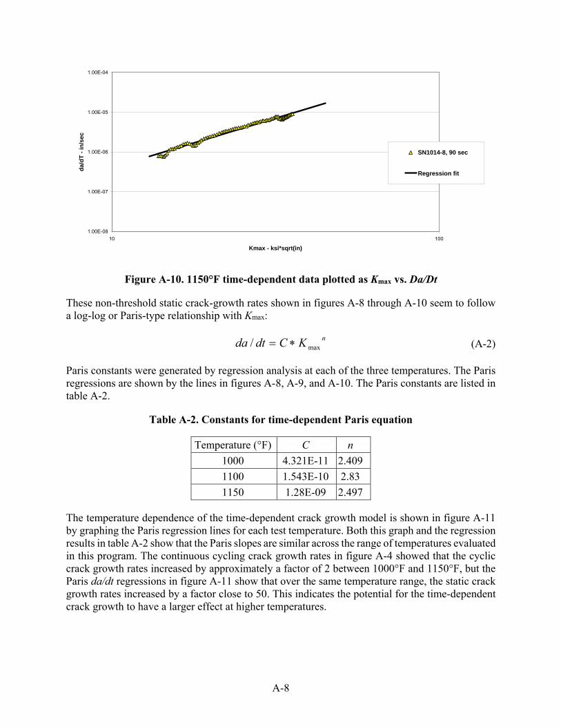
A-8

Figure A-10. 1150°F time-dependent data plotted as Kmax vs. Da/Dt

These non-threshold static crack-growth rates shown in figures A-8 through A-10 seem to follow a log-log or Paris-type relationship with Kmax:

(A-2)

Paris constants were generated by regression analysis at each of the three temperatures. The Paris regressions are shown by the lines in figures A-8, A-9, and A-10. The Paris constants are listed in table A-2.

Table A-2. Constants for time-dependent Paris equation

Temperature (°F) C n

1000 4.321E-11 2.409

1100 1.543E-10 2.83

1150 1.28E-09 2.497

The temperature dependence of the time-dependent crack growth model is shown in figure A-11 by graphing the Paris regression lines for each test temperature. Both this graph and the regression results in table A-2 show that the Paris slopes are similar across the range of temperatures evaluated in this program. The continuous cycling crack growth rates in figure A-4 showed that the cyclic crack growth rates increased by approximately a factor of 2 between 1000°F and 1150°F, but the Paris da/dt regressions in figure A-11 show that over the same temperature range, the static crack growth rates increased by a factor close to 50. This indicates the potential for the time-dependent crack growth to have a larger effect at higher temperatures.

1.00E-08

1.00E-07

1.00E-06

1.00E-05

1.00E-04

10 100

Kmax - ksi*sqrt(in)

da/

dT

- i

n/s

ec

SN1014-8, 90 sec

Regression fit

nKCdtda max/

A-9

Figure A-11. Temperature dependence of the time-dependent model

To assess the accuracy of the time-dependent superposition model, the residual or crack propagation life of each time-dependent specimen was back-predicted using the linear superposition model (equation A-1) with the time-dependent portion calculated using the Paris equation (equation A-2) and the constants in table A-2. In figure A-12, the experimental life is graphed versus the predicted life for each time-dependent specimen. Also shown in figure A-12 are a 1:1 correlation line and a 2X scatter band, which is an industry standard approach for assessment of cyclic crack propagation life prediction. All points fell within the 2X scatter band, and, on average, were in agreement with the 1:1 line. This indicates that the experimental lives were accurately predicted using the time-dependent model developed in this program. Note that all of the 1000°F tests fell well within the 2X scatter bands even though the one 3600-second hold time test in figure A-8 showed the variation previously discussed relative to the Paris regression.

Another representation of the back-predictions is shown in figure A-13. In this figure, the normalized life ratio (experimental life divided by predicted life) is graphed versus hold time. The figure shows that the model displays no bias as a function of temperature or hold time. Again the 1000°F, long hold time test showed some variation, but it was well within the desired 2X variation in predicted life.

In figure A-14, the predictions from figure A-12 were re-plotted along with a set of predictions using the continuous cycling curve only, which does not account for the time-dependent effects behavior. The cyclic predictions were greatly nonconservative and showed that the crack growth in each of these experiments was dominated by time-dependent contributions.

1.00E-08

1.00E-07

1.00E-06

1.00E-05

1.00E-04

10 100

Kmax - ksi*sqrt(in)

da/

dT

- in

/sec 1000F

1100F

1150F

A-10

Figure A-12. Experimental vs. predicted life plotted for all time-dependent specimens

Figure A-13. Normalized life ratio plotted vs. hold time for all time-dependent specimens

Alloy 718

10

100

1000

10000

10 100 1000 10000

Nexp

Np

red

1:1 Line

+/- 2X scatter band

1150F

1100F

1000F

0.1

1

10

10 100 1000 10000

Hold time (sec)

Nex

p/N

pre

d

+/- 2X scatter band1150F1100F1000F

A-11

Figure A-14. Experimental vs. predicted specimen lives using a superposition model or a cyclic crack-growth model

A.4 CRACK-GROWTH RETARDATION BEHAVIOR

A.4.1 CRACK-GROWTH RETARDATION TESTS

The crack-growth retardation test matrix is shown in table A-3. This matrix is a slight modification from the originally proposed matrix. These modifications were made because early test results were different from what was originally anticipated. This is not a total surprise because the original matrix was developed from estimated retardation constants with no Alloy 718 experimental data. These modifications will be discussed in more detail later in the report.

For this matrix, figure A-15 shows a schematic representation of the waveforms for the three types of tests that were performed: (a) a single OP test, (b) a multiple (“mission”) OP test, and (c) an “OP + hold” test. A single OP test (figure A-15a) has a single OP followed by a very large number of lower amplitude fatigue cycles to measure the size of the zone where a single OP reduces or retards the crack growth rate. Two or three of these single OP segments could be applied to a test specimen based on the magnitude of the OP and the available specimen dimensions, and this will be discussed in more detail later. The OP ratio was defined as S1/S2 for this test protocol (and also for the other two types of tests). A mission OP test (figure A-15b) is a simplified mission test with a pre-selected number of minor cycles (5, 10, or 20 minor cycles for this test matrix) before the next OP cycle is applied. In figure A-15b, the schematic shows a test for which five minor cycles follow each major cycle. An OP + hold test (figure A-15c) is a mission hold-time test for which an OP is applied prior to a hold at a lower stress for a specific time.

10

100

1000

10000

10 100 1000 10000

Nexp

Np

red

1:1 Line

+/- 2X scatter band

superposition model

cyclic model

A-12

Table A-3. Crack-growth retardation test matrix

Material Temp

(F) Test Type

OP Stress (ksi)

Cyclic / Hold

Stress (ksi)

OP (%)

Number of Minor Cycles

Hold Time (sec)

Number of Tests

Test Specimen

Fine Grain 718 (supplied by GEA)

450

Single OP

127.5 127.5

85 75

50 70

2 1

Large SC (Kb)

Multiple OP

127.5 127.5 127.5

98 85 85

30 50 50

5 5

10

1 1 1

Small SC (Kb)

1000

Single OP

127.5 127.5

85 75

50 70

2 1

Large SC (Kb)

Multiple OP

127.5 127.5 127.5

98 85 85

30 50 50

5 5

10

1 1 1

Small SC (Kb)

Hold OP

127.5 127.5 127.5

122.6 116

98

4 10 30

2400 1200 1200

1 1 1

Large SC (Kb)

1100

Single OP

127.5 127.5

85 75

50 70

2 1

Large SC (Kb)

Multiple OP

127.5 127.5 127.5

98 85 85

30 50 50

20 5

10

1 1 1

Small SC (Kb)

Hold OP

127.5 127.5 127.5

121.4 116 122.6

5 10 4

90 1200 900

1 1 1

Large SC (Kb)

A-13

(a) (b)

(c)

Figure A-15. Schematic representation of (a) a single OP waveform, (b) a multiple (“mission”) OP waveform, and (c) an “OP + hold” waveform

A.4.2 CRACK-GROWTH RETARDATION MODELING

The crack-growth retardation model used to describe these data was a modified Willenborg model developed by VanStone and Slavik [A-1]. This model was applied both to cyclic retardation (overloads with no hold times) and static retardation (overloads with hold times).

A.4.2.1 Cyclic Retardation

The cyclic retardation constants were determined using the method described by VanStone and Slavik [A-1]. The single OP test segments were used to generate the modified Willenborg constants , , and . In general, three of these OP test segments were performed on each 1.5 OP ratio specimen, and two OP test segments were performed on each 1.7 OP ratio specimen. The higher OP ratio reduces the number of segments per specimen because increasing OP ratios increases the size of the retardation zone.

Examples of the data obtained from a single OP cyclic retardation test can be seen in figures A-16 and A-17 for a 450°F and a 1000°F test, respectively. Also plotted in each figure is the predicted baseline cyclic crack-growth rate without the single OP. The crack-growth rate for the baseline prediction increased with crack depth because the tests were performed in load control and K increases with crack size. In both figures, the amount of crack extension (depth direction)

Alloy 718 Single Overpeak Cycle

Time (seconds)

Str

es

s (

ks

i)

Overpeak applied here

Baseline cycling continues as the crack grows through the retardation zone before the next overpeak is applied

S1S2

Alloy 718 Single Overpeak Cycle

Time (seconds)

Str

es

s (

ks

i)

Overpeak applied here

Baseline cycling continues as the crack grows through the retardation zone before the next overpeak is applied

S1S2

S1S2

Alloy 718 Mult OP Cycle

Time (seconds)

Str

es

s (

ks

i)

One cycle Repeats

Alloy 718 Overpeak + Hold Cycle

Time (seconds)

Str

ess

(ksi

)

One cycle Repeats

A-14

following application of the OP was plotted on the x-axis. The crack-growth rate is plotted on the y-axis. The retardation data showed the expected trends in behavior. The minimum in the crack-growth rate occurred at a small amount of crack extension following application of the OP. For both of these tests, the minimum in the crack-growth rate occurred after a crack extension of approximately 0.7 mil.

Figure A-16. Example of single OP cyclic retardation test data at 450°F

Alloy 718 450F

1.00E-07

1.00E-06

1.00E-05

0 0.005 0.01 0.015 0.02 0.025 0.03

A - Aop

da/

dN

- i

n/c

ycle

Baseline

1.7 Overpeak RatioAt application of OP, K(a) for overpeak = 36.1 ksi*sqrt(in)

Approach baseline behavior at end of retardation zone

Minimum crack growth rate at the max value of

Kreduced

Alloy 718 450F

1.00E-07

1.00E-06

1.00E-05

0 0.005 0.01 0.015 0.02 0.025 0.03

A - Aop

da/

dN

- i

n/c

ycle

Baseline

1.7 Overpeak RatioAt application of OP, K(a) for overpeak = 36.1 ksi*sqrt(in)

Approach baseline behavior at end of retardation zone

Minimum crack growth rate at the max value of

Kreduced

A-15

Figure A-17. Example of single OP cyclic retardation test data at 1000°F

The cyclic retardation constants , , and obtained from the analysis of the single OP test segments are reported in table A-4. The constant describes the distance beyond the OP where the minimum crack growth rate is observed. The constant describes the size of the OP zone (beyond which retardation is no longer observed). Both of these constants exhibited negligible temperature dependence, so a common value was used across all the temperatures evaluated in this program. The constant defines the trend of the reduced K as a function of the crack length within the retardation zone. The behavior defined by was consistent for a given temperature, and exhibited a temperature dependence shown in table A-4.

Table A-4. Cyclic retardation constants for modified Willenborg model

Temp

Cyclic constants

χ λ ρ

450 0.17 5.84 1.55

1000 0.17 5.84 4.15

1100 0.17 5.84 2.3 Mission OP tests were performed to determine the cyclic constant . The constant determines the magnitude of the crack-growth retardation. Increases in the value of result in higher retardation (lower values of K and, therefore, reduced crack-growth rates) and dominates the retardation life benefit. Using the constants , , and , the cyclic is the value that best back-predicts the crack propagation lives of the multiple cyclic mission OP test data at each

Alloy 718 1000F

1.00E-07

1.00E-06

1.00E-05

0 0.004 0.008 0.012

A - Aop

da/

dN

- in

/cyc

le

Baseline

1.5 Overpeak RatioAt application of OP, K(a) for overpeak = 23.6 ksi*sqrt(in)

Approach baseline behavior at end of retardation zone

Minimum crack growth rate at the max value of

Kreduced

Alloy 718 1000F

1.00E-07

1.00E-06

1.00E-05

0 0.004 0.008 0.012

A - Aop

da/

dN

- in

/cyc

le

Baseline

1.5 Overpeak RatioAt application of OP, K(a) for overpeak = 23.6 ksi*sqrt(in)

Approach baseline behavior at end of retardation zone

Minimum crack growth rate at the max value of

Kreduced

A-16

temperature. The cyclic retardation constant obtained from the analysis of the mission OP data is reported in table A-5. The variation of cyclic with test temperature is shown in figure A-18.

Table A-5. Calculated cyclic retardation constants for mission OP data

Temp (F) Cyclic Phi

450 0.56

1000 0.78

1100 0.76

Figure A-18. Values of the cyclic retardation constant plotted as a function of temperature

The cyclic retardation constants , , , and described above constitute the material properties needed to make cyclic crack-growth predictions with the modified Willenborg retardation model. To assess the accuracy of the model, the residual life of each mission OP specimen was back-predicted using the retardation model. In figure A-19, the experimental life is plotted versus the predicted life for each mission OP specimen. In the legend, the specific OP ratio and the number of minor cycles per major cycle are listed for each specimen. Also plotted in figure A-19 are a 1:1 correlation line and a 2X scatter band. All points fell within the 2X scatter band, and, on average, showed exceptional correlation between the predicted and observed lives. This indicates that the fine-grained Alloy 718 experimental lives were accurately predicted using the cyclic retardation model developed in this program.

0

0.2

0.4

0.6

0.8

1

400 600 800 1000 1200

Temp ( F)

Cyc

lic P

hi

Cyclic Phi

A-17

Figure A-19. Experimental versus predicted life plotted for each mission OP specimen. Specimen predictions were performed using a modified Willenborg retardation model

The back-predictions of these mission OP specimens are plotted again in figure A-20 using a common symbol. Also plotted in figure A-20 is a set of predictions for these specimens without the effect of retardation. Figure A-20 shows that the predictions with retardation not included were significantly conservative. Use of the modified Willenborg retardation model can help to remove excessive conservatism in predictions of missions with significant OPs.

Alloy 718 Cyclic Mission OP Tests

100

1000

10000

100 1000 10000

Nexp

Np

red

1:1 Line+ / - 2X scatter band450F, 1.3/5 minor450F, 1.5/5 minor450F, 1.5/10 minor1000F, 1.3/5 minor1000F, 1.5/5 minor1000F, 1.5/10 minor1100F, 1.3/20 minor1100F, 1.5/5 minor1100F, 1.5/10 minor

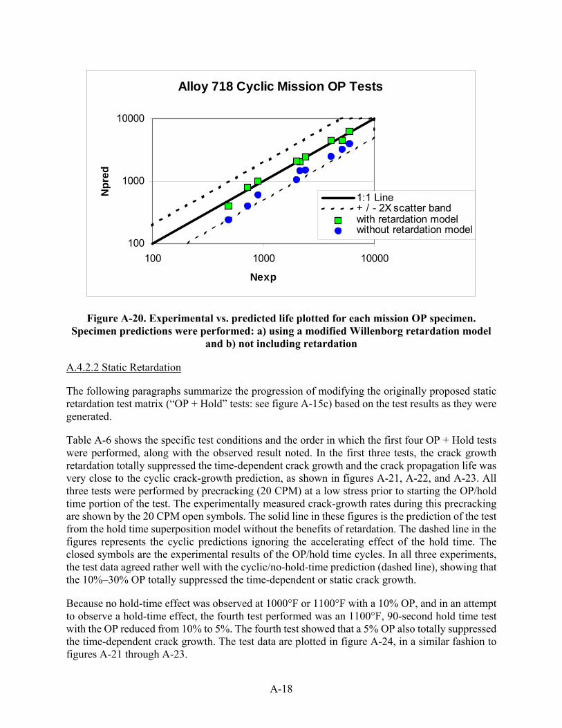
A-18

Figure A-20. Experimental vs. predicted life plotted for each mission OP specimen. Specimen predictions were performed: a) using a modified Willenborg retardation model

and b) not including retardation

A.4.2.2 Static Retardation

The following paragraphs summarize the progression of modifying the originally proposed static retardation test matrix (“OP + Hold” tests: see figure A-15c) based on the test results as they were generated.

Table A-6 shows the specific test conditions and the order in which the first four OP + Hold tests were performed, along with the observed result noted. In the first three tests, the crack growth retardation totally suppressed the time-dependent crack growth and the crack propagation life was very close to the cyclic crack-growth prediction, as shown in figures A-21, A-22, and A-23. All three tests were performed by precracking (20 CPM) at a low stress prior to starting the OP/hold time portion of the test. The experimentally measured crack-growth rates during this precracking are shown by the 20 CPM open symbols. The solid line in these figures is the prediction of the test from the hold time superposition model without the benefits of retardation. The dashed line in the figures represents the cyclic predictions ignoring the accelerating effect of the hold time. The closed symbols are the experimental results of the OP/hold time cycles. In all three experiments, the test data agreed rather well with the cyclic/no-hold-time prediction (dashed line), showing that the 10%–30% OP totally suppressed the time-dependent or static crack growth.

Because no hold-time effect was observed at 1000°F or 1100°F with a 10% OP, and in an attempt to observe a hold-time effect, the fourth test performed was an 1100°F, 90-second hold time test with the OP reduced from 10% to 5%. The fourth test showed that a 5% OP also totally suppressed the time-dependent crack growth. The test data are plotted in figure A-24, in a similar fashion to figures A-21 through A-23.

Alloy 718 Cyclic Mission OP Tests

100

1000

10000

100 1000 10000

Nexp

Np

red

1:1 Line+ / - 2X scatter bandwith retardation modelwithout retardation model

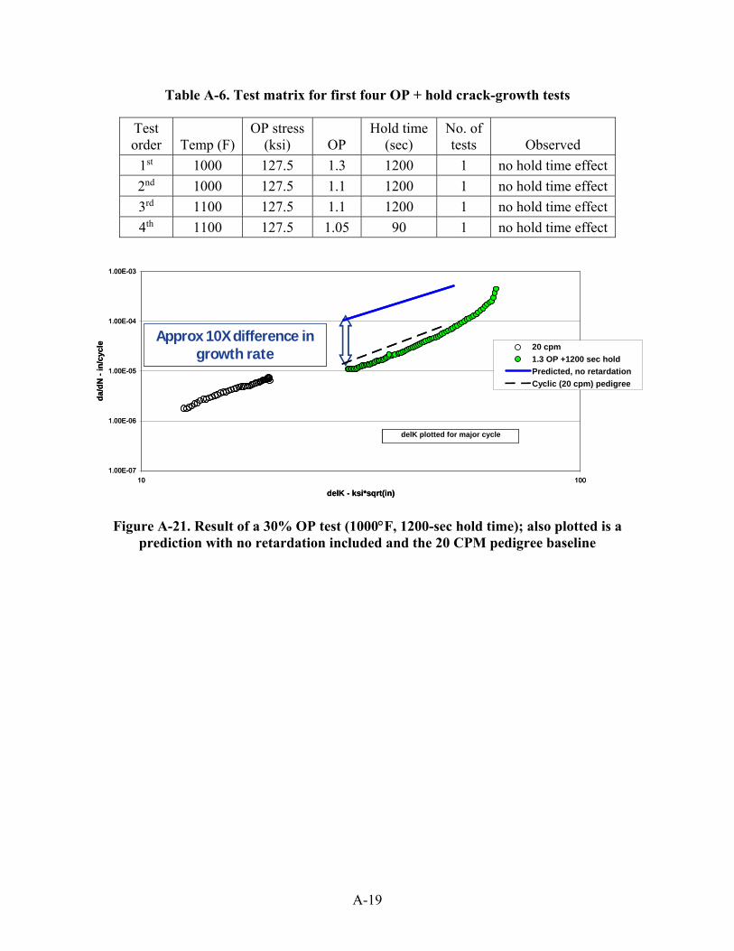
A-19

Table A-6. Test matrix for first four OP + hold crack-growth tests

Test order Temp (F)

OP stress (ksi) OP

Hold time (sec)

No. of tests Observed

1st 1000 127.5 1.3 1200 1 no hold time effect

2nd 1000 127.5 1.1 1200 1 no hold time effect

3rd 1100 127.5 1.1 1200 1 no hold time effect

4th 1100 127.5 1.05 90 1 no hold time effect

Figure A-21. Result of a 30% OP test (1000F, 1200-sec hold time); also plotted is a prediction with no retardation included and the 20 CPM pedigree baseline

Approx 10X difference in growth rate

1.00E-07

1.00E-06

1.00E-05

1.00E-04

1.00E-03

10 100

delK - ksi*sqrt(in)

da/

dN

- i

n/c

ycle 20 cpm

1.3 OP +1200 sec hold

Predicted, no retardation

Cyclic (20 cpm) pedigree

delK plotted for major cycle

Approx 10X difference in growth rate

1.00E-07

1.00E-06

1.00E-05

1.00E-04

1.00E-03

10 100

delK - ksi*sqrt(in)

da/

dN

- i

n/c

ycle 20 cpm

1.3 OP +1200 sec hold

Predicted, no retardation

Cyclic (20 cpm) pedigree

delK plotted for major cycle

A-20

Figure A-22. Result of a 10% OP test (1000°F, 1200-sec hold time); also plotted is a prediction with no retardation included and the 20 CPM pedigree baseline

Figure A-23. Result of a 10% OP test (1100°F, 1200-sec hold time); also plotted is a prediction with no retardation included and the 20 CPM pedigree baseline

1.00E-07

1.00E-06

1.00E-05

1.00E-04

1.00E-03

10 100

delK - ksi*sqrt(in)

da/

dN

- in

/cyc

le

20 cpm1.1 OP + 1200 sec holdPredicted, no retardationCyclic (20 cpm) pedigree

del K plotted for major cycle

Approx 10X difference in growth rate

1.00E-07

1.00E-06

1.00E-05

1.00E-04

1.00E-03

10 100

delK - ksi*sqrt(in)

da/

dN

- in

/cyc

le

20 cpm1.1 OP + 1200 sec holdPredicted, no retardationCyclic (20 cpm) pedigree

del K plotted for major cycle

Approx 10X difference in growth rate

1.00E-06

1.00E-05

1.00E-04

1.00E-03

1.00E-02

10 100

delK - ksi*sqrt(in)

da/

dN

- in

/cyc

le

20 cpm

1.1 OP + 1200 sec hold

Predicted, no retardation

Cyclic (20 cpm) pedigree

del K plotted for major cycle

Approx 45X difference in growth rate

1.00E-06

1.00E-05

1.00E-04

1.00E-03

1.00E-02

10 100

delK - ksi*sqrt(in)

da/

dN

- in

/cyc

le

20 cpm

1.1 OP + 1200 sec hold

Predicted, no retardation

Cyclic (20 cpm) pedigree

del K plotted for major cycle

Approx 45X difference in growth rate

A-21

Figure A-24. Result of a 5% OP test (1100F, 90-sec hold time); also plotted is a prediction with no retardation included and the 20 CPM pedigree baseline

Based on these results, an analytical sensitivity study was performed to select a combination of OP ratio and hold time that would discriminate the test result from both a cyclic (20 CPM) test and a hold time test (with no OP). Based on the predictions from the sensitivity study, the OP ratio for the remaining 1000°F test condition was reduced to 4%, and the hold time was increased to 2400 seconds. For the remaining 1100°F test, the OP ratio was reduced to 4%, and the hold time was increased to 900 seconds. The final modification of the matrix is shown in table A-7.

Table A-7. Test matrix for all OP + hold crack-growth tests

Test order Temp (F)

OP stress (ksi) OP

Hold time (sec)

No. of tests Observed

1st 1000 127.5 1.3 1200 1 no hold time effect

2nd 1000 127.5 1.1 1200 1 no hold time effect

3rd 1100 127.5 1.1 1200 1 no hold time effect

4th 1100 127.5 1.05 90 1 no hold time effect

5th 1100 127.5 1.04 900 1

6th 1000 127.5 1.04 2400 1 For these final two test specimens, three segments of cycling (each a different waveform) were performed on each specimen, as shown in figure A-25. The first segment was a 20 CPM continuously cycled test at a stress below the OP stress (127.5). The second segment of the test was a hold time cycle with the same stress as the hold time portion of the OP/hold test, which was 122.6 ksi (4% lower than 127.5 ksi). The final segment of the test was the 4% OP cycle. The crack growth rates measured in these two experiments can be seen in figures A-26 and A-27.

1.00E-06

1.00E-05

1.00E-04

1.00E-03

1.00E-02

10 100

delK - ksi*sqrt(in)

da/

dN

- in

/cyc

le 20 cpm

1.05 OP + 90 sec hold

Predicted, no retardation

Cyclic (20 cpm) pedigree

del K plotted for major cycle

Approx 5X difference in growth rate

1.00E-06

1.00E-05

1.00E-04

1.00E-03

1.00E-02

10 100

delK - ksi*sqrt(in)

da/

dN

- in

/cyc

le 20 cpm

1.05 OP + 90 sec hold

Predicted, no retardation

Cyclic (20 cpm) pedigree

del K plotted for major cycle

Approx 5X difference in growth rate

Approx 5X difference in growth rate

A-22

In these two experiments with a 4% OP, the retardation partially suppressed the time-dependent crack growth. For the OP + hold waveform, the fatigue cracks grew faster than those predicted from cyclic crack growth, but still significantly slower than that predicted for cyclic plus time-dependent crack growth without the benefit of the OP.

Figure A-25. Schematic representation of the three types of cycles used in the final two OP/hold retardation tests

Time (seconds)

Str

ess

(ksi

)

Time (seconds)

Str

ess

(ksi

)

One cycle Repeats

Time (seconds)

Str

es

s (

ks

i)

One cycle Repeats

Hold time stress the same for segments 2

and 3

1st segment (20 cpm)

2nd segment (hold time)

3rd segment (OP+hold)

Time (seconds)

Str

ess

(ksi

)

Time (seconds)

Str

ess

(ksi

)

One cycle Repeats

Time (seconds)

Str

es

s (

ks

i)

One cycle Repeats

Hold time stress the same for segments 2

and 3

Time (seconds)

Str

ess

(ksi

)

Time (seconds)

Str

ess

(ksi

)

One cycle Repeats

Time (seconds)

Str

es

s (

ks

i)

One cycle Repeats

Hold time stress the same for segments 2

and 3

1st segment (20 cpm)

2nd segment (hold time)

3rd segment (OP+hold)

A-23

Figure A-26. 1100°F crack-growth data from the same specimen using three different waveforms: a) 20 CPM baseline, b) 900-second hold time, and c) 4% OP with a 900 second

hold time

Figure A-27. 1000°F crack-growth data from the same specimen using three different waveforms: a) 20 CPM baseline, b) 2400-second hold time, and c) 4% OP with a

2400-second hold time

The “OP + hold” retardation test data were successfully modeled using the modified Willenborg retardation model [A-1]. The time-dependent or static retardation constants (i.e., “static ”) obtained from the analysis of these data are given in table A-8.

To assess the accuracy of the model, the residual life of each “OP + hold” specimen was back-predicted using the model. In figure A-28, the experimental life is plotted versus the predicted life for each specimen. Also plotted in the figure are a set of cyclic-only predictions and a set of predictions using the superposition model but without retardation. The figure also shows the

1.00E-06

1.00E-05

1.00E-04

1.00E-03

1.00E-02

10 100

del K - ksi*sqrt(in)

da/

dN

- in

/cyc

le

20 cpm

900 sec hold

1.04 OP + 900 sec hold

Cyclic (20 cpm) pedigree

del K plotted for major cycle

1.00E-06

1.00E-05

1.00E-04

1.00E-03

1.00E-02

10 100

del K - ksi*sqrt(in)

da/

dN

- i

n/c

ycle

20 cpm

2400 sec hold

1.04 OP + 2400 sec hold

Cyclic (20 cpm) pedigree

del K plotted for major cycle

A-24

customary 1:1 correlation line, and a 2X scatter band. The experiments with a 4% OP were accurately predicted using the combination of the hold-time superposition and static retardation models (closed triangles). The remaining four experiments were conservatively predicted using this same model. As stated previously, in these four experiments, the magnitude of the OP was sufficiently high to eliminate any crack-growth acceleration due to the hold time. It can also be seen from the figure that the “cyclic only” predictions (open squares) have the potential to be non-conservative; this was clearly demonstrated in the 1100°F test with the 4% OP that had an experimental crack-propagation life of 40 cycles. It was also shown that predictions without considering the benefits of static retardation (closed circles) can be extremely conservative.

Table A-8. Calculated static retardation constants for OP + hold data

Temp (F) Static Phi

1000 19.05

1100 10.9

Figure A-28. Experimental vs. predicted lives for the “OP + hold” specimens. Three sets of predicted lives are plotted: a) using a cyclic curve (“cyclic only”), b) the time-dependent

model, not including retardation (“static, no retard”), and C) including both the time-dependent and the retardation model (“static + retardation”)

A.5 SUMMARY

All of the objectives for the GEA time-dependent crack-growth program were achieved. Time-dependent crack-growth data and crack-growth retardation data were generated for fine-grained Alloy 718 over a range of temperatures important for gas turbine operations. Hold times and OPs were selected for the purpose of calibrating and validating the linear superposition model and the modified Willenborg retardation model. The crack-growth models were generated, and the hold

Alloy 718 OP + Hold Tests

1

10

100

1000

10000

1 10 100 1000 10000

Nexp

Np

red

1:1 Line+ / - 2X scatter bandCyclic onlyStatic, no retardStatic + retardation

4% OP + Hold tests are accurately predicted. Tests not used to determine the

constant (that is, the tests with larger overpeaks) are conservatively predicted.

Only the tests with a 4% overpeak are discerning tests

4% OP + Hold tests are accurately predicted. Tests not used to determine the

constant (that is, the tests with larger overpeaks) are conservatively predicted.

Only the tests with a 4% overpeak are discerning tests

A-25

time and retardation model constants were reported. The residual lives of the hold time tests from the time-dependent matrix were accurately predicted using the linear superposition model. The residual lives of the cyclic mission OP tests from the retardation matrix were accurately predicted using the modified Willenborg model. The residual lives of the “overpeak + hold” tests from the retardation matrix were accurately predicted using the modified Willenborg model.

A.6 REFERENCES

A-1. Van Stone, R.H. and Slavik, D.C. (2000). Prediction of Time-Dependent Crack Growth with Retardation Effects in Nickel Base Alloys. Fatigue and Fracture Mechanics, 31st Volume, ASTM STP 1389, (405–426). West Conshohocken, PA: ASTM International.

A-2. Van Stone, R.H. and Richardson, T.L. (1985). Potential Drop Monitoring of Cracks in Surface Flawed Specimens. Automated Test Methods for Fracture and Fatigue Crack Growth, ASTM STP 877, (148–166). West Conshohocken, PA: ASTM International.

B-1

APPENDIX B—A NEW ANALYSIS METHOD FOR TIME-DEPENDENT CRACK GROWTH

This appendix documents a new analysis method for time-dependent crack growth proposed by Pratt & Whitney (P&W) and a corresponding series of crack-growth experiments performed by P&W

08 to guide and evaluate the new methodology. The proposed method uses an equivalent stress intensity factor (SIF) in a superposition method to predict fatigue crack growth (FCG) at elevated temperatures. The formulation for the equivalent SIF was motivated by crack geometry and load history considerations.

B.1 EXPERIMENTS

B.1.1 TEST PROCEDURES

A series of time-dependent crack-growth tests were performed on double-melt fine-grain IN-718 to guide the development of the methodology. All specimens were machined from a supplier forging, supplier serial number 145, heat number A47466. The forging was solution heat treated and aged per P&W 1085 Specification. The typical yield stress for the material at 1200oF is 153 ksi.

Tests were performed at two temperatures (1100F and 1200F) and are summarized in table B-1. Three specimen geometries were used in the tests: compact tension (CT), surface flaw (SF), and bolt hole (BH). The specimen geometries and dimensions are shown in figure B-1. Four different load-time histories were employed: continuous cycling at 20 Hz and 10 CPM (0.167 Hz), so-called “2-minute dwell” tests (2mdw), and static crack-growth tests. In this report, “cyclic” crack growth denotes crack growth during load cycling, and “static” crack growth denotes crack extension under static load, which may result from environmental or creep mechanisms. Load profiles are characterized in figure B-2. Here tdwell is dwell time, which was 120 seconds for 2mdw tests, and zero for 10 CPM and 20 Hz cyclic tests. The time per cycle (denoted by tcycle) was 6 seconds for 10CPM loading, and 0.05 seconds for 20 Hz load cycle. For static crack-growth tests, the load was kept constant during testing, and the hold time tdwell was the same as the test time. Cyclic crack-growth tests were conducted at three different stress ratios: R = 0.1, 0.3, and 0.7. This test matrix was selected to provide a basis for development of time-dependent crack-growth models that account for temperature, stress ratio, load history, and constraint effects. An additional “mission” test was conducted for future validation efforts.

B-2

Table B-1. P&W test matrix for time-dependent crack growth

Load Conditions

R=0.1 R=0.3 R=0.7 R=1

Mission 10cpm 2mdw 2mdw 2mdw Creep

T=1100F 1 SF

1 SF 1 SF 1 SF 1 SF

1 SF 1 CT 1 CT

1 BH 2 BH

T=1200F 1 SF 1 SF 1 SF 1 SF 1 SF

1 CT 1 CT 1 CT

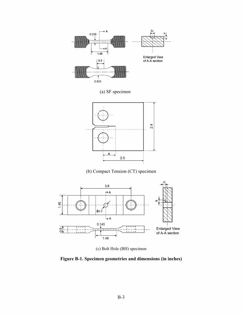
B-3

(a) SF specimen

(b) Compact Tension (CT) specimen

(c) Bolt Hole (BH) specimen

Figure B-1. Specimen geometries and dimensions (in inches)

B-4

(a) Dwell Loading Profile

(b) Cyclic load profile

Figure B-2. Load histories and nomenclature

All tests were conducted using standard FCG test methods in the P&W laboratory. The following maximum cyclic loads were applied to each specimen geometry: CT – 1,700 lbf, SF – 126 ksi, and BH – 16,700 lbf. The SIFs for the CT and SF specimens were calculated by well-known equations [B-1, B-2], and for the BH specimen by the fracture mechanics analysis software FRANC3D, as will be discussed later.

B.1.2 TEST RESULTS

First, all test results are summarized to document the effects of crack geometry, R-ratio, and load history on FCG at elevated temperatures. Because ΔK is widely assumed to dominate FCG, all

Time

App

lied

Load

tdwelltcycle

Time

App

lied

Load

tdwelltcycle

tcycle

Time

App

lied

Load

tcycle

Time

App

lied

Load

B-5

cyclic crack growth data (da/dN) are shown as functions of ΔK, whereas static crack-growth data (da/dt) are shown as functions of maximum K.

Figure B-3 shows the effect of stress ratio on crack-growth rates in 2mdw tests for SF specimens at two temperatures, 1100oF and 1200oF, and three R-ratios, 0.1, 0.3 and 0.7. The crack-growth rates increased substantially as R increased at the same ΔK values, suggesting that ΔK alone does not uniquely control time-dependent crack growth. Similar results for 2mdw tests from CT and BH specimens are shown in figures B-4 and B-5. The influence of R on crack-growth rate for these two geometries was similar to that observed for the SF specimen in figure B-3.

To explore whether crack-growth rates are more dominated by the maximum value of K for time-dependent crack growth, the 2mdw test results were re-plotted as a function of maximum K in figure B-6 for the SF specimen and in figure B-7 for the CT specimen. For both geometries, 2mdw crack-growth rates from different R-ratios showed a very weak R-ratio dependency, whereas 20 Hz crack growth rates increased as R increased at the same Kmax values.

The BH specimen introduced a number of complications. An initial quarter-circular corner notch (0.005″ × 0.005″) was electro-discharge machined in the BH specimen but not fatigue pre-cracked as for the SF and CT specimens. The BH crack-growth data used in model development was taken after the crack had grown four times larger (0.02″) than the initial notch size. The original corner crack changed its shape significantly with crack propagation, as shown in figure B-8 for a specimen at 1100F and R = 0.3. Note that the crack developed a complex tunneled shape as it grew. The crack radial depth, “a”, was recorded as a function of load cycles, as shown in figure B-9. Duplicate R = 0.3 tests were conducted and resulted in different crack-growth responses, even though the test conditions were nominally identical.

B-6

(a) (b)

Figure B-3. Two-minute dwell crack-growth rate as function of ΔK for SF specimen; (a): 1100oF and (b): 1200oF

1.E-06

1.E-05

1.E-04

1.E-03

1.E-02

1 10 100

2MDW, R=0.1

2MDW, R=0.3

2MDW, R=0.7

1100oFda

/dN

(in/c

ycle

)

∆K (ksiin)

1.E-06

1.E-05

1.E-04

1.E-03

1.E-02

1 10 100

2MDW, R=0.1

2MDW, R=0.3

2MDW, R=0.7

1100oFda

/dN

(in/c

ycle

)

∆K (ksiin)

1.E-06

1.E-05

1.E-04

1.E-03

1.E-02

1 10 100

2MDW, R=0.1

2MDW, R=0.3

2MDW, R=0.7

1200oF

da/d

N(in

/cyc

le)

∆K (ksiin)

1.E-06

1.E-05

1.E-04

1.E-03

1.E-02

1 10 100

2MDW, R=0.1

2MDW, R=0.3

2MDW, R=0.7

1200oF

da/d

N(in

/cyc

le)

∆K (ksiin)

B-7

(a) (b)

Figure B-4. Two-minute dwell crack-growth rate as function of ΔK for CT specimen; (a): 1100oF and (b): 1200oF

Figure B-5. Two-minute dwell crack-growth rate as function of ΔK for BH specimen

1.E-08

1.E-07

1.E-06

1.E-05

1.E-04

1.E-03

1.E-02

1 10 100

2MDW, R=0.1

2MDW, R=0.3

20Hz, R=0.1

20Hz, R=0.3

1100oF

da/d

N(in

/cyc

le)

∆K (ksiin)

1.E-08

1.E-07

1.E-06

1.E-05

1.E-04

1.E-03

1.E-02

1 10 100

2MDW, R=0.1

2MDW, R=0.3

20Hz, R=0.1

20Hz, R=0.3

1100oF

da/d

N(in

/cyc

le)

∆K (ksiin)1.E-09

1.E-08

1.E-07

1.E-06

1.E-05

1.E-04

1.E-03

1.E-02

1 10 100

20Hz, R=0.1

20Hz, R=0.3

2MDW, R=0.1

2MDW, R=0.3

1.E-07

1.E-06

1.E-05

1.E-04

1.E-03

1.E-02

10 100

2MDW,R=0.3

2MDW, R=0.3

2MDW, R=0.1

1100oF

da/d

N(in

/cyc

le)

∆K (ksiin)

1.E-07

1.E-06

1.E-05

1.E-04

1.E-03

1.E-02

10 100

2MDW,R=0.3

2MDW, R=0.3

2MDW, R=0.1

1100oF

da/d

N(in

/cyc

le)

∆K (ksiin)

B-8

(a) (b)

Figure B-6. Two-minute dwell crack-growth rate as function of maximum K for SF specimen; (a): 1100oF and (b): 1200oF

(a) (b)

Figure B-7. Two-minute dwell crack-growth rate as function of maximum K for CT specimen; (a): 1100oF and (b): 1200oF

Kmax (ksiin)

da

/dN

(in

/cyc

le)

1.E-06

1.E-05

1.E-04

1.E-03

1.E-02

1 10 100

10CPM, R=0.1

2MDW, R=0.1

2MDW, R=0.3

2MDW, R=0.7

1100oF

Kmax (ksiin)

da

/dN

(in

/cyc

le)

1.E-09

1.E-08

1.E-07

1.E-06

1.E-05

1.E-04

1.E-03

1.E-02

1 10 100

20Hz, R=0.1

20Hz, R=0.3

2MDW, R=0.1

2MDW, R=0.3

B-9

Figure B-8. Crack shape changes with crack growth for a BH specimen

Figure B-9. Crack depth vs. cycles data for BH specimens

0

0.05

0.1

0.15

0.2

0.25

0.3

0.35

0.4

0.45

0 200 400 600 800 1000 1200 1400

Cycles (N)

Cra

ck d

ep

th (

a)

15837, 2MDW, R=0.1 @1100F

15838, 2MDW, R=0.3 @1100F

15839, 2MDW, R=0.3 @1100F

B-10

An equation for the SIF of a tunneled crack at a hole is not available. The FRANC3D fracture-mechanics software was used to calculate the SIF with crack-shape change for the specific crack shapes observed in these tests. This numerical solution was used to calculate the elastic K values in figure B-5. The K value used was calculated at the point the crack depth “a” was measured. The BH specimen cracks were found to grow with similar aspect ratios as a function of crack depth, as shown in figure B-10, and this simplified the generation of K solutions.

Figure B-10. Changes in crack aspect ratio with crack depth for BH specimen

The loads applied to the BH specimen caused appreciable yielding at the edge of the hole. The nominal gross section maximum stress in the specimen was 79.4 ksi, and the peak elastic stress at the edge of the (uncracked) hole was estimated to be approximately 250 ksi. The 0.2% offset yield strength is nominally 153 ksi. An approximate time-independent shakedown calculation for the BH specimen without crack for a first load cycle indicated that loading to maximum stress would result in a much lower peak elastic-plastic tensile stress. Subsequent unloading to zero applied load would result in a local compressive residual stress of approximately 80 ksi at the edge of the uncracked hole. Therefore, the actual local stress ratio (Kmin/Kmax) for the initial crack would have been lower than the nominal applied stress ratio of R=0.1 or 0.3. If additional time-dependent yielding occurred at these high local stresses and temperatures (which is likely), the time-dependent plastic deformation would have developed further, the compressive residual stresses upon unloading would have been even larger, and the related local stress-ratio changes more pronounced. This local plastic deformation may have several other effects, including redistribution of the stress ahead of the notch and the stress ahead of the crack tip, which could in turn affect the crack growth rate.

0

1

2

3

4

0 0.1 0.2 0.3 0.4 0.5

#15838

#15839

Asp

ect

ratio

a/c

Crack depth a (in)

0

1

2

3

4

0 0.1 0.2 0.3 0.4 0.5

#15838

#15839

Asp

ect

ratio

a/c

Crack depth a (in)

B-11

Furthermore, it should be noted that the large stresses applied to the specimen would have caused significant plasticity in the remaining ligament as the crack grew. The remaining ligament on the cracked side of the hole would nominally have been fully plastic by the time the crack length reached approximately a = 0.25″. This plasticity may have caused some load shedding from the cracked side of the hole to the uncracked side of the hole, thereby reducing the driving force for crack extension below nominal values.

Application of crack-growth-rate data from a particular specimen type to engine components requires that the data be expressed in a geometry-independent form, or that the specimen and component share the same critical geometry features. To understand if the time-dependent crack-growth data could be uniquely characterized by the SIF K for different geometries, the crack-growth rates from different specimens were re-plotted in terms of ΔK at identical test conditions (2mdw, 1100F) in figure B-11. The CT specimen generally exhibited slightly faster growth than the SF specimen, whereas the crack-growth rates in the BH specimens were approximately 10 times slower than the CT and SF rates.

Time-dependent crack growth at elevated temperatures is generally understood to be influenced by the combined effects of fatigue, creep, and environmental attack. These interactions may change with load history. To study the effects of load history, three static crack-growth tests were conducted with SF or CT specimens at 1100F and 1200F. Static crack-growth rates da/dt (crack increment per unit time, inches/second) are shown as a function of K in figure B-12. This static crack-growth rate represents one limiting case for time-dependent crack growth if the load is kept constant (the hold time at peak load is very long). The other limiting case for time-dependent crack growth is a high-frequency cyclic load for which the time period per cycle is very short, creep and environmental attacks are very limited, and crack growth can be regarded as a purely fatigue process. In this investigation, the limiting case for the high-frequency cyclic load was taken to be 20 Hz.

Time-dependent crack-growth results are summarized in figures B-13 and B-14 for four load history types and two temperatures. In these figures, the crack-growth rate is da/dN (crack growth per cycle) for cyclic loads (20 Hz, 10 CPM, and 2mdw) and da/dt for static loads (crack growth per second). The correlating parameter here is Kmax. These results suggest that time-dependent crack growth may not be a simple sum of time-independent cyclic crack growth and time-dependent static crack growth.

B-12

(a) (b)

Figure B-11. Two-minute dwell crack growth rates in different specimens at 1100oF; (a): R = 0.1 and (b): R = 0.3

Figure B-12. Static crack growth rate as function of K

1.E-07

1.E-06

1.E-05

1.E-04

1.E-03

1.E-02

1 10 100

2MDW, SF

2MDW, CT

2MDW, BH

R=0.1

da/d

N(in

/cyc

le)

∆K (ksiin)

1.E-07

1.E-06

1.E-05

1.E-04

1.E-03

1.E-02

1 10 100

2MDW, SF

2MDW, CT

2MDW, BH

R=0.1

da/d

N(in

/cyc

le)

∆K (ksiin)

1200oF

1.E-07

1.E-06

1.E-05

1.E-04

1.E-03

1.E-02

1 10 100

2MDW, CT

2MDW, SF

2MDW, BHa

2MDW, BHb

R=0.3

da/d

N(in

/cyc

le)

∆K (ksiin)

1200oF

1.E-07

1.E-06

1.E-05

1.E-04

1.E-03

1.E-02

1 10 100

2MDW, CT

2MDW, SF

2MDW, BHa

2MDW, BHb

R=0.3

da/d

N(in

/cyc

le)

∆K (ksiin)

1.E-08

1.E-07

1.E-06

1.E-05

1.E-04

1.E-03

1 10 100

CT, 1200F

SF, 1200F

SF, 1100F

da/d

t(in

/sec

ond)

K (ksiin)

1.E-08

1.E-07

1.E-06

1.E-05

1.E-04

1.E-03

1 10 100

CT, 1200F

SF, 1200F

SF, 1100F

da/d

t(in

/sec

ond)

K (ksiin)

B-13

(a) (b)

Figure B-13. The effects of load history on crack growth rate at 1100F; (a): R = 0.1 and (b): R = 0.3

(a) (b)

Figure B-14. The effects of load history on crack growth rate at 1200F; (a): R = 0.1 and (b): R = 0.3

1.E-08

1.E-07

1.E-06

1.E-05

1.E-04

1.E-03

1.E-02

1 10 100

10CPM, SF

2MDW, SF

2MDW, CT

20Hz, CT

Creep, SF

da/d

N,

da/d

t

Kmax (ksiin)

R=0.1

da/dt

1.E-08

1.E-07

1.E-06

1.E-05

1.E-04

1.E-03

1.E-02

1 10 100

10CPM, SF

2MDW, SF

2MDW, CT

20Hz, CT

Creep, SF

da/d

N,

da/d

t

Kmax (ksiin)

R=0.11.E-08

1.E-07

1.E-06

1.E-05

1.E-04

1.E-03

1.E-02

1 10 100

10CPM, SF

2MDW, SF

2MDW, CT

20Hz, CT

Creep, SF

da/d

N,

da/d

t

Kmax (ksiin)

R=0.1

da/dt

1.E-08

1.E-07

1.E-06

1.E-05

1.E-04

1.E-03

1.E-02

1 10 100

2MDW, CT

2MDW, SF

20Hz, CT

Creep, SF

Kmax (ksiin)da

/dN

, da

/dt

R=0.3

1.E-08

1.E-07

1.E-06

1.E-05

1.E-04

1.E-03

1.E-02

1 10 100

2MDW, CT

2MDW, SF

20Hz, CT

Creep, SF

Kmax (ksiin)da

/dN

, da

/dt

R=0.3

da/dt

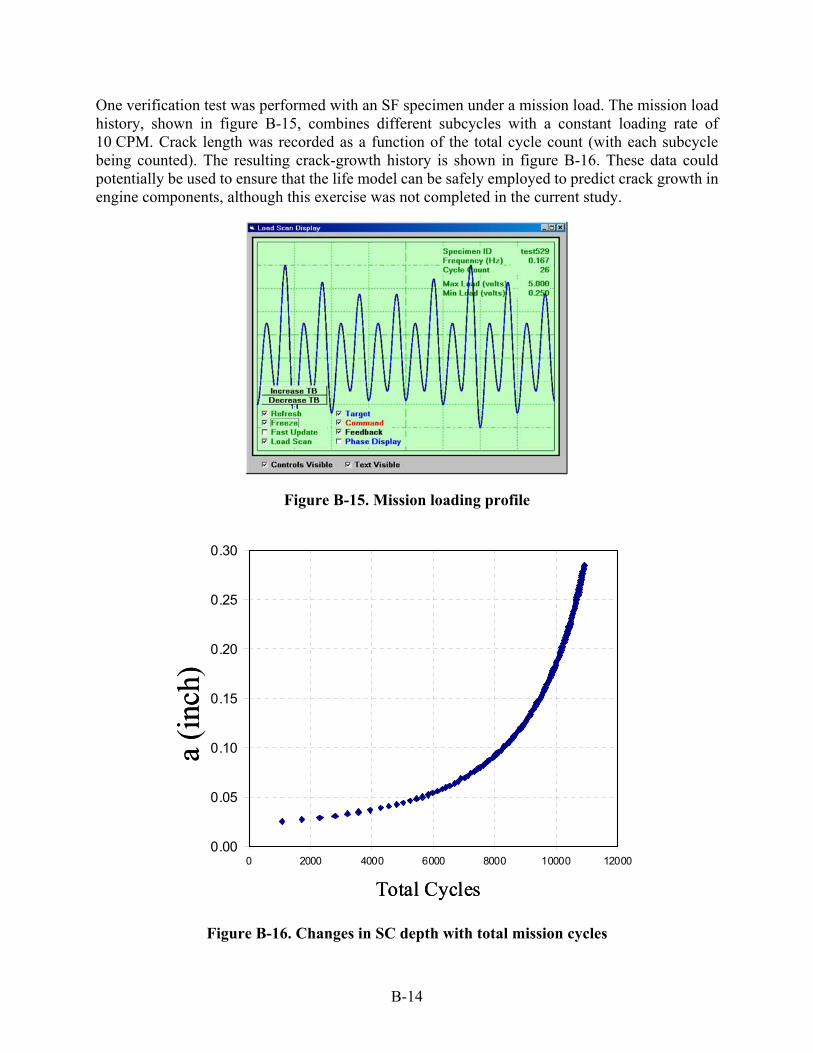
B-14

One verification test was performed with an SF specimen under a mission load. The mission load history, shown in figure B-15, combines different subcycles with a constant loading rate of 10 CPM. Crack length was recorded as a function of the total cycle count (with each subcycle being counted). The resulting crack-growth history is shown in figure B-16. These data could potentially be used to ensure that the life model can be safely employed to predict crack growth in engine components, although this exercise was not completed in the current study.

Figure B-15. Mission loading profile

Figure B-16. Changes in SC depth with total mission cycles

0.00

0.05

0.10

0.15

0.20

0.25

0.30

0 2000 4000 6000 8000 10000 12000

Total Cycles

a (i

nch)

0.00

0.05

0.10

0.15

0.20

0.25

0.30

0 2000 4000 6000 8000 10000 12000

Total Cycles

a (i

nch)

B-15

B.2 AN EFFECTIVE SIF FOR TIME-DEPENDENT FCG

These test data indicated that crack-growth rates and the crack-growth threshold depended on crack geometry and load history. In particular, the BH specimen exhibited significantly different crack-growth rates from the SF and CT specimens. The goal of the methodology development effort in this task is to explain (and ultimately to predict) these geometry and load history effects.

The approach taken here was limited to small-scale yielding (SSY) problems in which the elastic SIF K can be used as the fundamental characteristic crack-tip parameter. In general, plastic deformation and creep can develop in the crack-tip region during time-dependent crack growth. In some cases, however, the crack-tip inelastic zone is small enough that it is adequately contained by the surrounding elastic deformation, and this is assumed to be the case here.

Figure B-17 is a schematic representation of the evolution of local stress and strain at the crack tip for time-dependent crack growth. Although appreciable tensile plastic deformation may occur initially, the local time-dependent cyclic behavior that controls crack growth will often be elastic in nature.

Figure B-17. Schematic representation of stress cycle at the crack tip for inelastic time-dependent material response

However, it is sometimes not the case that a single parameter adequately describes the crack-tip fields and the related crack-tip damage. Previous research in time-independent and time-dependent elastic-plastic fracture mechanics employing the J-integral [B-4] and C(t) [B-5] integrals as correlating parameters indicated that an additional parameter [B-6, B-7] may be needed to properly characterize the near-tip field when the constraint required by single-parameter fracture mechanics is lost because of inelastic deformation. Second parameters—such as the T-stress [B-8, B-9], Q-stress [B-10, B-11], and triaxial stress [B-12, B-13]—have been proposed.

Str

ess

Strain

Crack

B-16

In sections B.2.1-B.2.3, an effective SIF parameter is derived to scale the stress in the crack-tip region. The time-independent plastic effect is addressed with a constraint loss parameter, whereas the time-dependent effect is addressed with an approach motivated by creep considerations.

B.2.1 PLASTIC-ZONE-RELATED CONSTRAINT PARAMETER

The plastic zone near the crack tip can be strongly affected by the nature of the surrounding elastic field arising from the remote load, even under SSY conditions. For example, for plane crack problems, the elastic stress field generally scales with the SIF, but is also influenced by the so-called T-stress, which is the non-singular stress in a direction parallel to the crack. Changes in T-stress can lead to significant changes in both the size and shape of the crack-tip plastic zone [B-8, B-9]. The T-stress approach is an easy way to characterize plastic zone effects on elastic-plastic crack problems under SSY conditions because it uses strictly elastic parameters.

To evaluate whether this approach could be used to characterize the observed dependency of FCG on geometry, the T-stress was calculated using published equations for the SF and CT specimens [B-14, B-15] and using the FRANC3D fracture mechanics software for the BH specimen. The T-stresses were calculated at threshold conditions (initial crack sizes). The initial K values (so-called Kthreshold) for the three specimens are plotted against the calculated T-stress values in figure B-18. However, these T-stress values were not well-correlated with observed crack growth behavior. The SF and CT specimens exhibited very similar crack-growth rates but very different T-stress values, whereas the BH specimen (which might have been expected to have a highly negative T-stress value, based on the observed crack growth rates) actually had a calculated T-stress value similar to the CT specimen. From these results, it was concluded that T-stress was not an appropriate constraint parameter to correlate the threshold for time-dependent crack growth.

Figure B-18. Changes in K-threshold with normalized T-stress by yield stress

0

5

10

15

20

25

30

‐1 ‐0.8 ‐0.6 ‐0.4 ‐0.2 0 0.2

Calculated

Expected

Kth

resh

old

Ts/

CT

BH BH

SF

B-17

This result prompted the search for an alternative parameter that could be used consistently in characterization of constraint changes in crack growth for both plane crack problems and 3D crack problems. It is well known that plastic deformation is the root cause of crack-tip constraint loss. This is also consistent with the earlier observation that extensive plastic deformation likely occurred in the BH specimen, which exhibited significantly different crack-growth rates from the SF and CT specimens with much less plasticity.

The development of plastic zone shape and size depends on both crack geometry and loads, so constraint is a function of crack geometry and load. In fact, several research groups have claimed that the stresses in different crack geometries can be characterized by plastic zone size [B-12, B-16, B-17]. In the present work, it was postulated that the normalized plastic zone length, Lp, along the crack growth direction could be used to characterize the effects of crack geometry on crack growth rate. Here the plastic zone length has been normalized by the SIF and the yield stress according to the form:

(B-1)

where Rp is the actual plastic zone length along the crack-growth direction and is yield stress.

To evaluate this postulate, an FEA for plastic zone length was performed using ANSYS with J2-flow theory for all three specimen geometries (CT, SF and BH). For simplicity, a bi-linear hardening rule was used in this analysis, with a Young’s modulus of 26,500 ksi, a yield stress of 153 ksi, and a hardening modulus of 190 ksi, which is similar to a typical hardening exponent of n = 10 for the Ramberg-Osgood relationship. The ANSYS models explicitly modeled the crack at its initial position at the beginning of the test (initial crack size and shape). The Lp values were not recomputed at larger crack sizes corresponding to later times in the tests.

From the numerical result, the plastic zone length, Rp, was defined as the distance from the crack tip to the point on the crack-growth path at which the effective plastic strain was greater than 10-5. The nondimensional plastic zone length Lp was calculated from equation B-1. Threshold (initial) Kmax values for the three specimens were plotted as a function of Lp in figure B-19. More testing would be required to confirm the shape of the function, but from the plot of Kthreshold versus Lp, it appears that the change of Lp over three specimens is generally consistent with the dependence of threshold value on specimen geometry. Therefore, the plastic zone length, LP, might be capable of characterizing the change of crack-growth rate with crack geometry.

In this part of the formulation, we are considering only the stress intensity for the first few cycles of time-dependent load, for which time-dependent effects have not yet begun. Here, the development of plastic deformation in the crack-tip region depends on the maximum load. Analogous to Q-stress and T-stress (e.g., [11]), we define here an effective plastic SIF Kep as:

(B-2)

20K

RL p

p

0

pep Q

KK

B-18

where Qp is a function of the constraint parameter Lp. Qp is unity when Lp is zero, and increases as Lp increases. The effective SIF is postulated to control crack initiation (threshold) and growth for different crack geometries without load history effects.

Figure B-19. Changes in K-threshold with Lp

As the crack grows, the plastic zone size changes, leading to increases in Qp. To simplify the problem, we rewrite Qp as:

(B-3)

where Qthreshold is defined as the Qp value at the initial (threshold) condition of K= Kthreshold. Qgrowth represents the change in Qp with crack growth. Both Qthreshold and Qgrowth are postulated to be functions of the constraint parameter Lp.

B.2.2 EFFECTS OF LOADING HISTORY ON EFFECTIVE SIF

As the loading frequency decreases, creep and oxidation attacks increase, and crack growth is controlled by time-dependent mechanisms instead of cycle-dependent mechanisms. It is assumed here that the peak stress in the inelastic stress cycle can be related to the creep crack-tip parameter, the C(t)-integral [B-5, B-18]. C(t) is written here as a function of the effective plastic SIF Kep and a time-dependent term as:

(B-4)

where Qc is a function of the creep time td. Riedel and Rice [B-18] have proposed an approximate function for Qc. For time-dependent crack-growth problems, the creep effect is more complex.

0

5

10

15

20

25

30

0 1 2 3 4

Kth

resh

old

Lp

CT

BH

SF

GrowthQ

thresholdthresholdp K

KQQ

2dcepd tQKtC

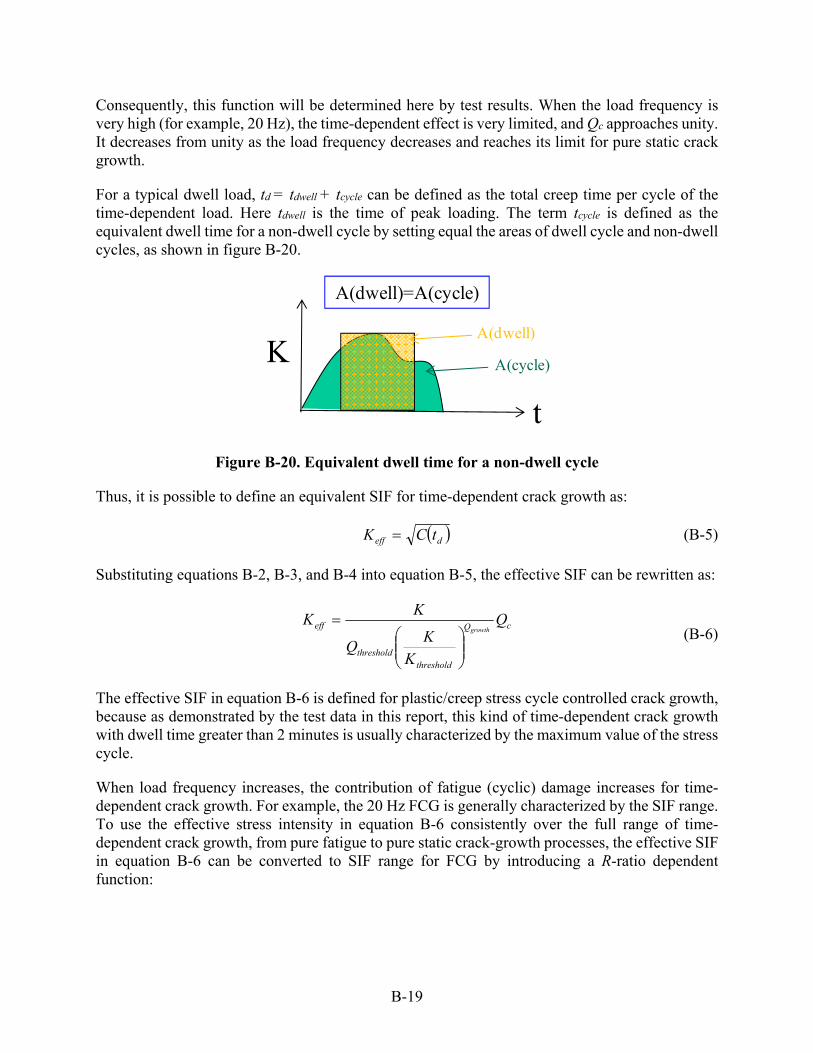
B-19

Consequently, this function will be determined here by test results. When the load frequency is very high (for example, 20 Hz), the time-dependent effect is very limited, and Qc approaches unity. It decreases from unity as the load frequency decreases and reaches its limit for pure static crack growth.

For a typical dwell load, td = tdwell + tcycle can be defined as the total creep time per cycle of the time-dependent load. Here tdwell is the time of peak loading. The term tcycle is defined as the equivalent dwell time for a non-dwell cycle by setting equal the areas of dwell cycle and non-dwell cycles, as shown in figure B-20.

Figure B-20. Equivalent dwell time for a non-dwell cycle

Thus, it is possible to define an equivalent SIF for time-dependent crack growth as:

(B-5)

Substituting equations B-2, B-3, and B-4 into equation B-5, the effective SIF can be rewritten as:

(B-6)

The effective SIF in equation B-6 is defined for plastic/creep stress cycle controlled crack growth, because as demonstrated by the test data in this report, this kind of time-dependent crack growth with dwell time greater than 2 minutes is usually characterized by the maximum value of the stress cycle.

When load frequency increases, the contribution of fatigue (cyclic) damage increases for time-dependent crack growth. For example, the 20 Hz FCG is generally characterized by the SIF range. To use the effective stress intensity in equation B-6 consistently over the full range of time-dependent crack growth, from pure fatigue to pure static crack-growth processes, the effective SIF in equation B-6 can be converted to SIF range for FCG by introducing a R-ratio dependent function:

t

K

A(dwell)=A(cycle)

A(dwell)

A(cycle)

deff tCK

cQ

thresholdthreshold

eff Q

K

KQ

KK

growth

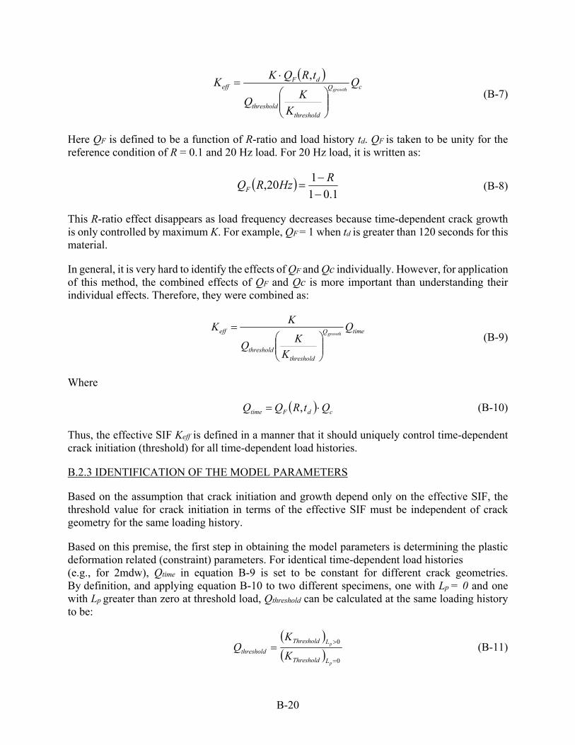
B-20

(B-7)

Here QF is defined to be a function of R-ratio and load history td. QF is taken to be unity for the reference condition of R = 0.1 and 20 Hz load. For 20 Hz load, it is written as:

(B-8)

This R-ratio effect disappears as load frequency decreases because time-dependent crack growth is only controlled by maximum K. For example, QF = 1 when td is greater than 120 seconds for this material.

In general, it is very hard to identify the effects of QF and Qc individually. However, for application of this method, the combined effects of QF and Qc is more important than understanding their individual effects. Therefore, they were combined as:

(B-9)

Where

(B-10)

Thus, the effective SIF Keff is defined in a manner that it should uniquely control time-dependent crack initiation (threshold) for all time-dependent load histories.

B.2.3 IDENTIFICATION OF THE MODEL PARAMETERS

Based on the assumption that crack initiation and growth depend only on the effective SIF, the threshold value for crack initiation in terms of the effective SIF must be independent of crack geometry for the same loading history.

Based on this premise, the first step in obtaining the model parameters is determining the plastic deformation related (constraint) parameters. For identical time-dependent load histories (e.g., for 2mdw), Qtime in equation B-9 is set to be constant for different crack geometries. By definition, and applying equation B-10 to two different specimens, one with Lp = 0 and one with Lp greater than zero at threshold load, Qthreshold can be calculated at the same loading history to be:

(B-11)

cQ

thresholdthreshold

dFeff Q

K

KQ

tRQKK

growth

,

1.01

120,

R

HzRQF

timeQ

thresholdthreshold

eff Q

K

KQ

KK

growth

cdFtime QtRQQ ,

0

0

p

p

LThreshold

LThreshold

threshold K

KQ

B-21

Therefore, Qthreshold can be obtained by fitting test results with different specimen geometries but the same loading history. It is unity for a specimen with Lp = 0, and it is expected to increase as Lp

increases.

After Qthreshold is determined in this manner, the threshold value of the crack-growth rate characterized by the effective SIF is identical for different crack geometries. However, the slope of the crack-growth rate curve depends on the crack-growth constraint function, Qgrowth. For a reference specimen with zero plastic deformation, Lp = 0 and Qgrowth = 0. As Lp increases, Qgrowth increases, and the crack-growth slope decreases. By fitting the crack-growth-rate data for Lp > 0 to match the data for Lp = 0 data by adjusting Qgrowth, Qgrowth can be determined for the specimen.

Figure B-21 shows the procedure used to determine Qthreshold and Qgrowth as functions of Lp for the CT and BH specimens for a 2mdw load history. Because Lp is always close to zero for the CT specimen, the threshold value and crack-growth-rate date were taken as reference for Qthreshold and Qgrowth (i.e., Qthreshold = 1 and Qgrowth = 0 for the CT specimen). For the BH specimen, LP is significantly greater than for the CT specimen. Therefore, Qthreshold and Qgrowth for the BH specimen can be obtained from crack growth data as shown in figure B-21. For SF specimens, the same procedure can be applied, and the functions for Qthreshold and Qgrowth can be obtained, as shown in table B-2. Note that the threshold values for BH and SF were estimated by comparing the region II test data to comparable CT specimen data.

Next, the load-history-related parameters are determined. In general, the development of time-dependent effects in the crack-tip region depend on load frequency and R-ratio. The reference condition to determine Qtime is taken to be R = 0.1 and 20 Hz load. The threshold value for the CT specimen (Lp = 0) is,

(B-12) HzLKK pthresholdthresholdeff 20 ;0

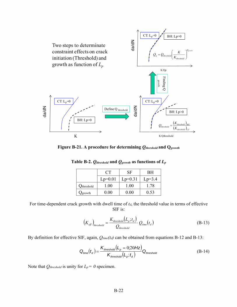
B-22

Figure B-21. A procedure for determining Qthreshold and Qgrowth

Table B-2. Qthreshold and Qgrowth as functions of Lp

CT SF BH

Lp=0.01 Lp=0.31 Lp=3.4

Qthreshold 1.00 1.00 1.78

Qgrowth 0.00 0.00 0.53 For time-dependent crack growth with dwell time of td, the threshold value in terms of effective

SIF is:

(B-13)

By definition for effective SIF, again, Qtime(td) can be obtained from equations B-12 and B-13:

(B-14)

Note that Qthreshold is unity for Lp = 0 specimen.

K

CT: Lp=0

da

/dN

BH: Lp>0

CT: Lp=0

da

/dN

BH: Lp>0

K/Qthreshold

CTthreshold

BHthresholdthreshold K

KQ

CT: Lp=0

da

/dN

BH: Lp>0

K/Qp

growthQ

thresholdthresholdp K

KQQ

Define Q threshold

Find

ing Q

growth

Two steps to determinate constraint effects on crack initiation (Threshold) and growth as function of Lp

dtimethreshold

dpthreshold

thresholdeff tQQ

tLKK

;

threshold

dpthreshold

pthresholddtime Q

tLK

HzLKtQ

;

;200

B-23

Therefore, Qtime(td) can be determined by fitting equation B-14 to test data from identical specimens with different loading histories. Table B-3 summarizes the Qtime(td) values thus determined for temperatures of 1100oF and 1200oF, respectively. Note that the red numbers in these tables were estimated by interpolation, and the blue numbers were calculated based on the assumption that ΔK is the dominant parameter for time-independent FCG.

Table B-3(a). Variation of Qtime with loading history at T = 1100oF

R 20Hz 10 CPM 2 MDW Creep

0.1 1.00 0.87 0.65 0.51

0.3 0.79 0.72 0.65 0.51

0.7 0.33 0.49 0.65 0.51

Table B-3(b). Variation of Qtime with loading history at T = 1200oF

R 20Hz 10 CPM 2 MDW Creep

0.1 1.00 0.87 0.63 0.53

0.3 0.79 0.71 0.63 0.53

0.7 0.33 0.48 0.63 0.53

In summary, the effective SIF includes both Qtime and Qp. Here Qtime represents the time-dependent effects, and Qp represents the constraint effects. By definition, the crack-growth rate must be independent of crack geometry and load history in terms of this effective SIF. Therefore, if the load history is the same (Qtime is same), any difference in the two crack-growth rates results from Qp. Based on this difference, Qp (Qthreshold and Qgrowth) can be determined from test results. For crack-growth rates from different load histories for the same specimen (Qp is same), different threshold values will be adjusted by Qtime to the same value, which is the threshold value in terms of effective SIF. Additional experimental investigations would be required to verify the independence of these parameters.

B.3 TIME-DEPENDENT CRACK GROWTH MODEL.

Using the effective stress intensity defined in section B.2, time-dependent crack growth is assumed to be the sum of contributions from cyclic (fatigue) crack growth and static crack growth. This can be written as:

(B-15)

Here it is assumed that both terms on the right side of equation B-15 are functions of effective stress intensity. If this is true, the time-dependent crack-growth model should work equally well for time-dependent crack growth throughout the range of time scales (for example, 20 Hz, 10 CPM, 2mdw, and static crack growth) and for various crack geometries because the effective SIF defines a threshold that should be independent of cycle duration and crack geometry. It is also independent of R-ratio because this effect has been included in the effective SIF. This is the main

CycleFatiguedependentTime

dtdt

da

dN

da

dN

da

B-24

difference of the proposed time-dependent crack-growth model compared to the widely used simple superposition method in terms of K alone.

With Keff assumed to be the driving force for time-dependent crack growth, Priddle’s FCG model [B-19] can be written as:

(B-16)

where ΔKth is the threshold for FCG, and Kf is the critical value of Keff for unstable crack growth. Both a and p are material constants.

The static crack-growth rate is given by:

(B-17)

where Kth is the threshold for static crack growth, and Kc is the critical value for unstable static crack growth. Both b and q are material constants.

The time-dependent crack-growth rate is a combined static-cyclic problem, and the static mechanisms interact with the cyclic mechanisms. To account for this interaction, an additional interaction term is introduced into the static crack-growth model as:

(B-18)

where and are temperature-dependent material constants.

From P&W test data, the temperature-dependent material constants in equations B-16 and B-18 are summarized in table B-4.

Table B-4. Temperature-dependent material constants in equations B-16 and B-18

Temperature a p ΔKth Kf b q Kth Kc γ β

1100°F 4.70E-05 0.99 7.30 185.0 2.10E-04 1.30 8.30 130.0 0.55 2.00E-03

1200°F 5.50E-05 0.90 7.50 185.0 1.60E-03 1.33 8.30 190.0 0.71 6.90E-03

p

efff

theff

Fatigue KK

KKa

dN

da

q

effc

theff

KK

KKb

dt

da

d

q

effc

theff tKK

KKb

dt

da

exp1

B-25

With the cyclic crack-growth rate and static crack-growth rate defined in equation B-16 and equation B-18, respectively, the total time-dependent crack-growth rate can be obtained from equation B-15 as:

(B-19)

This proposed new time-dependent crack-growth model uses an effective SIF Keff to replace the original K as a crack-growth driving force. Keff includes the effects of crack geometry through the Qthreshold and Qgrowth parameters, whereas the Qtime parameter accounts for different loading history effects. The model first uses plastic constraint parameter Qthreshold and Qgrowth to adjust time-dependent crack-growth data so that it is identical for different crack geometries and then uses Qtime to adjust the time-dependent crack growth threshold to the same value for different load histories. Finally, superposition is used to obtain the total time-dependent crack growth.

To characterize time-dependent crack growth, the crack-growth model, equation B-19, must be calibrated from test data. Figure B-22 shows the crack-growth data for R = 0.1 and T = 1200oF for 20 Hz loading, static loading, and 2mdw loading. Crack growth rate da/dN (crack increment per cycle for fatigue and time-dependent crack growth) and da/dt (crack increment per second for static crack growth) are plotted as functions of the effective SIF, so they are independent of crack geometry and have identical thresholds. The material constants associated with these three equations were determined with the following procedures:

The first step is to calibrate the cyclic crack-growth model, equation B-14, from cyclic crack-growth data. Cyclic crack-growth results from pure cyclic loading for which the loading cycle time is short, so Qtime = 1, and time-dependent mechanisms do not contribute significantly to crack growth. Therefore, equation B-19 is reduced to a regular FCG model, equation B-16. In this case, 20 Hz of test data were used as pure cyclic crack-growth data. Material constants a, p, Kf, and Kth in equation B-14 were determined by fitting equation B-16 to the 20 Hz crack-growth data, as shown in figure B-22. Note that Qp = 1 because the data are from the CT specimen (Lp is close to zero).

Next, the static crack growth model, equation B-13, can be calibrated using static crack-growth data. By fitting equation B-13 to static test data in figure B-22, b, q, Kc, and Kth were determined. The static crack-growth model, equation B-17, is included in this figure for comparison.

The last step is to identify the interaction term in equation B-15. The remaining undetermined material constants in the time-dependent crack-growth model, equation B-15, are and . The 2mdw and 10 CPM crack growth data were used to identify the material constants by fitting equation B-15. Two intermediate times between the pure fatigue (20 Hz) data and the pure static data are needed to fit these constants.

It should be noted that all the currently available test data were used to calibrate this model. All of the comparisons in the following figures are therefore calibrations. No predictions have been performed. Additional testing and analysis would be required to validate the predictive capability of this approach.

Cycle

d

q

effc

theff

q

c

theff

dependentTime

dttKK

KKb

KK

KKa

dN

da)exp(1

max

B-26

Figure B-22. Effective SIF characterized crack-growth data for T = 1200oF and R = 0.1, and different crack model fittings

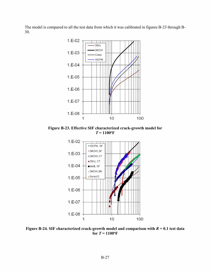
B-27

The model is compared to all the test data from which it was calibrated in figures B-23 through B-30.

Figure B-23. Effective SIF characterized crack-growth model for T = 1100oF

Figure B-24. SIF characterized crack-growth model and comparison with R = 0.1 test data for T = 1100oF

B-28

Figure B-25. SIF characterized crack-growth model and comparison with R = 0.3 test data for T = 1100oF

Figure B-26. SIF characterized crack-growth model and comparison with R = 0.7 test data for T = 1100oF

B-29

Figure B-27. Effective SIF characterized crack-growth model for T = 1200oF

Figure B-28. SIF characterized crack-growth model and comparison with R = 0.1 test data for T = 1200oF

B-30

Figure B-29. SIF characterized crack-growth model and comparison with R = 0.3 test data for T = 1200oF

Figure B-30. SIF characterized crack-growth model and comparison with R = 0.7 test data for T = 1200oF

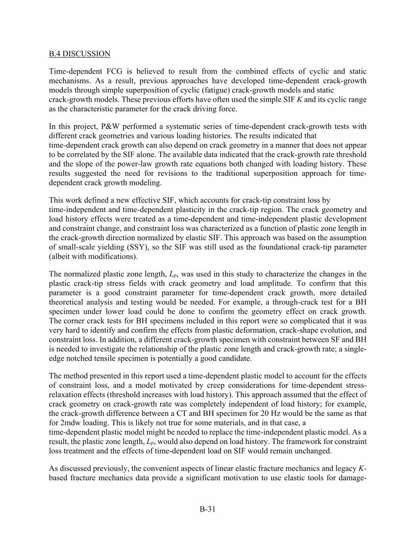
B-31

B.4 DISCUSSION

Time-dependent FCG is believed to result from the combined effects of cyclic and static mechanisms. As a result, previous approaches have developed time-dependent crack-growth models through simple superposition of cyclic (fatigue) crack-growth models and static crack-growth models. These previous efforts have often used the simple SIF K and its cyclic range as the characteristic parameter for the crack driving force.

In this project, P&W performed a systematic series of time-dependent crack-growth tests with different crack geometries and various loading histories. The results indicated that time-dependent crack growth can also depend on crack geometry in a manner that does not appear to be correlated by the SIF alone. The available data indicated that the crack-growth rate threshold and the slope of the power-law growth rate equations both changed with loading history. These results suggested the need for revisions to the traditional superposition approach for time-dependent crack growth modeling.

This work defined a new effective SIF, which accounts for crack-tip constraint loss by time-independent and time-dependent plasticity in the crack-tip region. The crack geometry and load history effects were treated as a time-dependent and time-independent plastic development and constraint change, and constraint loss was characterized as a function of plastic zone length in the crack-growth direction normalized by elastic SIF. This approach was based on the assumption of small-scale yielding (SSY), so the SIF was still used as the foundational crack-tip parameter (albeit with modifications).

The normalized plastic zone length, Lp, was used in this study to characterize the changes in the plastic crack-tip stress fields with crack geometry and load amplitude. To confirm that this parameter is a good constraint parameter for time-dependent crack growth, more detailed theoretical analysis and testing would be needed. For example, a through-crack test for a BH specimen under lower load could be done to confirm the geometry effect on crack growth. The corner crack tests for BH specimens included in this report were so complicated that it was very hard to identify and confirm the effects from plastic deformation, crack-shape evolution, and constraint loss. In addition, a different crack-growth specimen with constraint between SF and BH is needed to investigate the relationship of the plastic zone length and crack-growth rate; a single-edge notched tensile specimen is potentially a good candidate.

The method presented in this report used a time-dependent plastic model to account for the effects of constraint loss, and a model motivated by creep considerations for time-dependent stress-relaxation effects (threshold increases with load history). This approach assumed that the effect of crack geometry on crack-growth rate was completely independent of load history; for example, the crack-growth difference between a CT and BH specimen for 20 Hz would be the same as that for 2mdw loading. This is likely not true for some materials, and in that case, a time-dependent plastic model might be needed to replace the time-independent plastic model. As a result, the plastic zone length, Lp, would also depend on load history. The framework for constraint loss treatment and the effects of time-dependent load on SIF would remain unchanged.

As discussed previously, the convenient aspects of linear elastic fracture mechanics and legacy K-based fracture mechanics data provide a significant motivation to use elastic tools for damage-

B-32

tolerance analysis and design. As a result, elastic stress-based constraint parameters are preferred over plastic analysis-based parameters. This philosophy argues against the use of the plastic zone length (Lp) as a characteristic crack-tip parameter. A preliminary analysis indicated that it may be possible to use an elastic stress at a K-normalized distance ahead of the crack tip to replace the normalized plastic zone length as a constraint parameter. Figure B-31 suggests that this stress could be related to the normalized plastic zone length. If true, this substitution would render the method more practical for industrial application. However, it should be noted that calculation of either the plastic parameter Lp or the normalized elastic stress ahead of the crack would require a three-dimensional FEA of the cracked body (which could be a complex component) at a sufficient level of mesh refinement to provide sufficient accuracy, and without the results being sensitive to mesh refinement and other modeling parameters. This analysis step is not currently included in conventional damage-tolerance analyses; it would require substantial additional numerical effort to derive and validate the method, and to apply it to actual components.

Figure B-31. The variation of normalized plastic zone length with elastic stress at a normalized distance ahead of the crack tip

It should also be noted that tests with more complicated geometries and longer dwell time are lacking. These tests would be needed to further evaluate the validity of the proposed life model. Comparisons to mission loading data (see again figures B-15 and B-16) are also needed.

B.5 REFERENCES

B-1. Newman, J. C., Jr., and Raju, I. S. (1984). Stress-Intensity Factor Equations for Cracks in Three-Dimensional Finite Bodies Subjected to Tension and Bending Load. NASA Technical Memorandum 85793, NASA Langley Research Center, Hampton, VA.

B-2. Anderson, T. L. (1995). Fracture Mechanics: Fundamentals and Applications (2nd Ed.), Boca Raton, FL: Taylor & Francis Group, LLC, CRC Press.

B-33

B-3. Ma, F., Lehmann, D, and Morrison, T. (2009). The Effects of Loading History and Crack Geometry on Time-Dependent Fatigue Crack Growth at Elevated to High Temperatures. Paper presented at the 12th International Conference on Fracture, Ottawa, Canada.

B-4. Rice, J. R. (1968). A Path Independent Integral and the Approximate Analysis of Strain Concentrations by Notches and Cracks. Journal of Applied Mechanics, 35(2), 379–386.

B-5. Bassani, J. L. and McClintock, F. A. (1981). Creep Relaxation of Stress Around a Crack Tip. International Journal of Solids and Structures, 17(5), 479–492.

B-6. Hancock, J. W., Reuter, W. G. and Parks, D. M. (1993). Constraint and Toughness Parameterized by T. Constraint Effects in Fracture, ASTM STP 1171, (21–40). West Conshohocken, PA: ASTM International.

B-7. Roose, E., Eisele, U. and Silcher, H. (1993). Effects of Stress State on the Ductile Fracture Behavior of Large-Scale Specimens. Constraint Effects in Fracture, ASTM STP 1171, (41–63). West Conshohocken, PA: ASTM International.

B-8. Larsson, S. G. and Carlsson, A. J. (1973). Influence of Non-Singular Stress Terms and Specimen Geometry on Small-Scale Yielding at Crack-Tip in Elastic-Plastic Materials. Journal of the Mechanics and Physics of Solids, 21(4), 263–278.

B-9. Rice, J. R. (1974). Limitations to the Small Scale Yielding Approximation for Crack Tip Plasticity. Journal of the Mechanics and Physics of Solids, 22(1), 17–26.

B-10. O’Dowd, N. P. and Shih, C. F. (1991). Family of Crack-Tip Fields Characterized by a Triaxiality Parameter; Part I—Structure of Fields. Journal of the Mechanics and Physics of Solids, 39(8), 989–1015.

B-11. O’Dowd, N. P. and Shih, C. F. (1992). Family of Crack-Tip Fields Characterized by a Triaxiality Parameter; Part II —Fracture Applications. Journal of the Mechanics and Physics of Solids, 40(5), 939–963.

B-12. Ma, F., Sutton M. A., and Deng, X. (2001). Plane Strain Mixed Mode Crack-Tip Stress Fields Characterized by a Triaxial Stress parameter and a Plastic Deformation Extent Based Characteristic Length. Journal of the Mechanics and Physics of Solids, 49(12), 2921–2953.

B-13. Betegon, C. and Hancock, J. W. (1991). Two-Parameter Characterization of Elastic-Plastic Crack–Tip Fields. ASME Journal of Applied Mechanics, 58(1), 104–110.

B-14. Wang, X. (2002). Determination of Weight Functions for Elastic T-Stress from Reference T-Stress Solutions. Fatigue and Fracture of Engineering Materials and Structures, 25(10), 965–973.

B-15. Sherry, A. H., France, C.C., and Goldthorpe, M.R. (1995). Compendium of T-Stress Solutions for Two and Three Dimensional Cracked Geometries. Fatigue and Fracture of Engineering Materials and Structures, 18(1) 141–155.

B-34

B-16. Varias, A. G. and Shih, C. F. (1993). Quasi-Static Crack Advance Under a Range of Constraints Steady-State Fields Based on a Characteristic Length. Journal of the Mechanics and Physics of Solids, 41(5), 835–861.

B-17. Mostafavi, M., Smith D. J., and Pavier, M. J. (2009). Quantification of Constraint Effects in Fracture Mechanism Transition for Cracked Structures under Mixed Mode Loading. Fatigue and Fracture of Engineering Materials and Structures, 32(1) 5–17.

B-18. Riedel, H. and Rice, J. R. (1980). Tensile Crack in Creeping Solids. Fracture Mechanics: Proc. Twelfth National Symposium on Fracture Mechanics, ASTM STP 700, (112–130) West Conshohocken, PA: ASTM International.

B-19. Priddle, E. K. (1976). High Cycle Fatigue Crack Propagation under Random and Constant Amplitude Loadings. International Journal of Pressure Vessels and Piping, 4(2), 89–117.

C-1

APPENDIX C—ANALYTICAL MODELS FOR THERMO-MECHANICAL FATIGUE WITH HOT COMPRESSIVE CYCLES

A stress-level sensitivity approach is proposed for negative R-ratio cycles. This is applicable to isothermal or thermo-mechanical fatigue (TMF) loaded cracks but has special implications for hot compressive TMF. Following a discussion of these time-independent effects, test data associated with time-dependent effects are addressed, integrating crack-growth rate and creep results from other phases of the program. This requires use of an IN-718 crack-growth model produced from data developed under this program. However, because Design Assessment of Reliability With INspection (DARWIN®) did not support stress-level sensitivity at the time of this research, the crack growth model used to make predictions here did not employ stress level sensitivity methods. C.1 NEGATIVE R-RATIO MODELING.

Imagine simulating a physical crack-growth problem numerically using FEA for a cracked body cycling under tension-compression loading. This is typically referred to as the “negative R” regime, because R is nominally defined as σmin/σmax. However, R is more generally defined as Kmin/Kmax because a meaningful value of σmin/σmax is not easily defined for bodies with stress gradients. Note, however, that Kmin as calculated by FEMs will never achieve negative values when contact conditions on the crack faces are included, as demanded by the physics of the actual crack-growth problem. In these situations, the (elastic) physical simulation must give Kmin = 0, and, therefore, R = 0. In this situation, the conventional formulation of the Newman closure equations [C-1] fails to give the correct amount of crack closure. Although it is possible to obtain a fictitious negative Kmin by removing the contact boundary conditions of the crack in the FEA, this can cause errors in nearby contact or displacement boundary conditions and does not correspond to any real physical behavior. A suitable R-ratio cannot, in general, be defined for this class of problems, suggesting that it might be an inappropriate parameter for analysis of compressive cycle problems even in special cases for which it can be defined on a stress basis.

Arguments about the meaning of Kmin for negative loading are by no means new. For example, the consensus ASTM Standard Test Method E647 for measurement of fatigue crack-growth (FCG) rates, originally developed more than 30 years ago, declines to define negative Kmin values for negative loads, instead defining K = Kmax when the nominal R < 0. However, in the laboratory, an acceleration of crack growth is observed for compressive minimum stresses in comparison to true R = 0 (Smin = 0) load conditions, suggesting a sensitivity to compressive stress level at the crack tip. This will now be discussed in the context of the Newman closure model.

First, it is postulated here that stress level effects at positive and negative loads arise from two distinct mechanisms—a far field stress mechanism that occurs when the crack is open and a residual stress “neutralization” mechanism that occurs when the crack is globally closed. The far-field stress effect is revealed by the Dugdale model [C-2] for a center cracked panel (figure C-1), which predicts that the plastic zone grows infinite as the far field stress approaches the flow stress.

C-2

Figure C-1. Schematic of the Dugdale model for a center cracked infinite plate

This approach, while only valid for open cracks in a center cracked infinite panel, can be used to estimate both the maximum stress and cyclic plastic-zone dimensions associated with positive R-ratio cycles, motivating the use of Smax/S0 and Smin/S0 as relevant similarity parameters, or more customarily, Smax/S0 and R. Newman’s FASTRAN strip yield model [C-1] includes additional capability to handle crack closure beginning at the tip of the crack and the nonlinear contact aspect of the problem as closure moves back along the crack during unloading, compressing the expanded material that acts like a wedge in the crack. Some compressive stress neutralization is therefore included at this stage, but to the degree that the crack is open, the local stress and strain in the vicinity of the crack tip is driven by far-field loading more than by local loading.

Assuming a cycle such that the crack continues to unload until the crack becomes globally closed (presumably at Kelastic = 0), the contact nonlinearity associated with the gradually closing crack is no longer present. For a given material, the normalized state of residual stress, Sij/S0 may be presumed to be completely determined at that point by Smax/S0. Any further residual stress neutralization at the crack tip as the crack is now put into global compression is presumably caused by the local elastic compressive stress, Smin(a), superimposed on the residual stress. Therefore, the associated normalized similarity parameter is Smin(a)/S0. For the strip yield model a uniform far field stress is assumed, but the generalization of this as a local elastic stress seems to be a reasonable first approximation for small scale yielding, as shown in figure C-2.

Figure C-2. Schematic of the stress neutralization effect for a globally closed crack

Unlike Smax/S0, which represents a global loading condition only valid for a center cracked panel, Smin(a)/S0 may be considered more generally as a crack tip parameter for the compressive loading regime. While rejecting closure as a phenomenon, Lang [C-3] suggested nearly as much by proposing that stress-ratio effects be plotted in the modified format shown in figure C-3. Here, the Newman steady-state closure expressions have been plotted in standard format and in “Lang space,” showing that closure as currently formulated by Newman is more tightly collapsed in Lang space.

S0

2a

S0

2a

02cos

S

S

a

a

Smin(elastic) Residual stress zone before

compression

After compression

C-3

(a) (b)

Figure C-3. Newman closure equations for different normalized stress levels in standard R-ratio form (a), and lang space (b), Showing better collapse in lang space

Note also that in Lang space there is no longer any need to specify Kmin. This is equivalent to re-writing the Newman closure equations as:

(C-1)

Smin(a) is defined as the actual elastic “stress” at the crack tip location at the most compressive point in the cycle. For the present, we will assume this to be the stress normal to the globally closed crack (neglecting biaxial effects), either extracted from the first contact node back from the crack tip on the crack flank, or taken from an uncracked model with the same boundary conditions. In calculating Smin(a)/S0, the actual flow stress should be used (this usually is approximated by the average of the typical yield and ultimate stress, with C = 1, but the yield stress could be used with C > 1).

Smax/S0 is more difficult to define for general cases, where the applied stress is not uniform on the crack plane. An alternative approach employing Kmax/K0 has been proposed in the literature [C-4] but has not yet been fully validated. However, it is common in engineering software for FCG analysis to neglect the effect of Smax/S0 (typically by selecting Smax/S0 to be a constant value, sometimes user-specified). Because the effect of Smax/S0 on FCG rates is relatively small for

12

1

0071.415.

071.415.

2cos05.34.825.

0),(

)(/

13

312

max1

1

max2

33

221

min1max

AAA

AAAA

RforSS

crackclosedforA

S

SA

RforRRARARAAMAX

crackclosedforSaSCAASS

o

o

o

oo

o

ooop

C-4

tension-tension cycling (positive R values), this simplification should be adequate in the present development.

C.2 EFFECT OF STRESS-LEVEL SENSITIVITY ON TIME-INDEPENDENT HOT COMPRESSIVE TMF

Note that the flow stress is a function of temperature, and under TMF loading, the temperatures at max and min loads may differ. Therefore, the flow stress associated with the temperature of the compressive stress condition Tcomp should be used in the calculation of Smin(a)/S0. This will represent time-independent change in predicted crack-growth rate between isothermal and TMF loading (albeit a small change in most situations).

Also, any residual stress neutralization that occurs at Tcomp will be associated with a change in the residual strain distribution. Although the residual strain distribution does not change with a uniform shift in temperature, the stresses associated with it do scale with the elastic modulus, which does vary with temperature, suggesting the need for some adjustment based on the modulus ratio associated with the temperature range of the load cycle. Because it is based on ideal elastic-plastic behavior, however, the Dugdale model and its implementation in FASTRAN are independent of a modulus. Therefore, temperature effects on closure due to modulus changes will be neglected at this time.

C.3 TIME-DEPENDENT TMF WITH HOT COMPRESSIVE DWELL

C.3.1 CREEP SHAKEDOWN APPROACH

High-temperature dwell has sometimes been viewed in the literature in much the same way, regardless of whether the high temperature occurs during a tensile or compressive portion of the load cycle. Observed crack-growth acceleration has usually been attributed to oxidation or diffusion mechanisms [C-5]. However, smooth sample (surface flaw) isothermal crack-growth data for IN-718 developed under this program does not show any acceleration associated with the compressive dwell, suggesting that these environmental mechanisms are not dominant (at least not time-dependent) at the conditions tested (figure C-4).

C-5

Figure C-4. Comparison of 10 CPM and 2-min compressive dwell crack-growth data in IN-718, along with a corresponding NASGRO® equation model

1.E-10

1.E-09

1.E-08

1.E-07

1.E-06

1.E-05

1.E-04

1.E-03

1.E-02

10 100 1000Delta K Applied

da /

dN

IN718TRMD Modelat T = 1150°F and R = -2.167Specimen 15819A, 10 CPMSpecimen 15818A, 2 Min Comp Dwell

60 ksi

Stress (Load Controlled)

6 sec 2 min 6 sec

TD - TMF No TD- TMF

60 ksi

-130 ksi

Stress (Load Controlled)

6 sec 2 min 6 sec

TD - TMF No TD- TMF

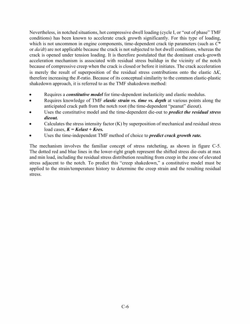
C-6

Nevertheless, in notched situations, hot compressive dwell loading (cycle I, or “out of phase” TMF conditions) has been known to accelerate crack growth significantly. For this type of loading, which is not uncommon in engine components, time-dependent crack tip parameters (such as C* or da/dt) are not applicable because the crack is not subjected to hot dwell conditions, whereas the crack is opened under tension loading. It is therefore postulated that the dominant crack-growth acceleration mechanism is associated with residual stress buildup in the vicinity of the notch because of compressive creep when the crack is closed or before it initiates. The crack acceleration is merely the result of superposition of the residual stress contributions onto the elastic K, therefore increasing the R-ratio. Because of its conceptual similarity to the common elastic-plastic shakedown approach, it is referred to as the TMF shakedown method:

Requires a constitutive model for time-dependent inelasticity and elastic modulus. Requires knowledge of TMF elastic strain vs. time vs. depth at various points along the

anticipated crack path from the notch root (the time-dependent “peanut” dieout). Uses the constitutive model and the time-dependent die-out to predict the residual stress

dieout. Calculates the stress intensity factor (K) by superposition of mechanical and residual stress

load cases, K = Kelast + Kres. Uses the time-independent TMF method of choice to predict crack growth rate.

The mechanism involves the familiar concept of stress ratcheting, as shown in figure C-5. The dotted red and blue lines in the lower-right graph represent the shifted stress die-outs at max and min load, including the residual stress distribution resulting from creep in the zone of elevated stress adjacent to the notch. To predict this “creep shakedown,” a constitutive model must be applied to the strain/temperature history to determine the creep strain and the resulting residual stress.

C-7

Figure C-5. Creep shakedown associated with hot compressive, time-dependent TMF

C.3.2 CONSTITUTIVE MODEL DEVELOPMENT

Before continuing, it should be noted that although, in general, the residual stress accumulates over a range of temperatures, it can be simulated isothermally at a high temperature if the dwell time in tension is reduced to minimize time-dependent effects when the crack is open. For demonstration of the mechanism, isothermal conditions were selected, requiring characterization of creep at only a single temperature (1150F).

Creep relaxation tests were conducted under both cyclic and static strain-controlled conditions, with limit strains corresponding to an initial target stress of 150 ksi allowing the stress to relax over time. These creep relaxation tests were conducted in tension, because an initial attempt to perform the tests in compression at -150 ksi resulted in specimen buckling. It is common to apply tensile creep data to compression problems.

C-8

Data for two successful tests are shown in figure C-6, showing a pronounced difference between cyclic and constant strain creep. Such a large difference was not expected and cannot be attributed to the small difference in max stress actually achieved during the tests. Although it would have been beneficial to be able to duplicate this important result, in the absence of further data, a simple constitutive model that fit the cyclic data was chosen for use in the simulation.

Note that the data are graphed as a residual stress, which accumulates over time, and they were fit to power law creep models that best correlated the observed behavior. For this purpose, the residual stress reported for the ith timepoint is given by:

(C-2)

Here εitest is the imposed instantaneous strain, i

test is the instantaneous stress measured during the test, and E(T) is the elastic modulus corresponding to the test temperature (which in this case is constant).

Figure C-6. Difference in creep behavior between constant strain and cyclic strain loading

The instantaneous stress can be expressed as a result of elastic and inelastic strain components:

(C-3)

)(TEtesti

testi

residuali

1150F1150F

150 ksi

-60 ksi

Elastic stress (strain controlled)

6 sec 2 min

0

10

20

30

40

50

60

70

1 10 100 1000 10000Neq, Equivalent 2 min

TMF Cycles

(Co

mp

ress

ive

) R

esi

du

al S

tre

ss,

ksi .

Specimen 16c-1 (147.7ksi max elastic s tress)Steady Creep ModelSpecimen 16c-2 (143.7 ks i max elastic s tress)Cyclic Creep Model

Constant Strain Test (Creep Relaxation)

2 Min Dwell Cyclic Strain Test

itcreepmech

iii dtE0

C-9

where the creep rate is a function of temperature and time (at least for simple models). For the present isothermal study, a power law model for the creep rate was assumed:

(C-4)

Equation C-5 can then be evaluated numerically, with t = 0 defined when the test load is first applied. The predicted instantaneous residual stress is given by:

(C-5)

By optimizing the parameters in equation C-4 to achieve the best fit, the models in figure C-7 were obtained.

Figure C-7. Creep models for constant strain and cyclic strain loading

C.3.3 NOTCHED FCG TESTS

To evaluate the performance of the method, two notched IN-718 FCG tests were performed at 1150F, one with a 2-minute compressive dwell, and one at 10 CPM. Both tests employed the fixed-grip double-edge-notch (DEN) specimen geometry and the load cycle shown in figure C-8. To provide adequate time for significant inelastic shakedown to occur at the notch, as would happen if cycling was required to initiate a fatigue crack, both specimens were pre-cycled with their respective cycle types for 2000 cycles prior to inserting an approximately 0.005-inch radius

nC

it

creepresiduali dtE

0

max

1.E-09

1.E-08

1.E-07

1.E-06

1.E-05

1.E-04

1.E-03

100 1000Stress (ksi)

Cre

ep S

trai

n ra

te (

1/h

r)

Steady Creep Model

Cyclic Creep Model

65.44)99613.2( Ec

87.19)4579.4( Ec

C-10

semicircular laser preflaw. The laser preflaw was selected because of its tendency to initiate crack growth almost immediately under subsequent cycling because of its highly sharpened geometry, and because it has almost no recast layer at the notch tip. The laser preflaws are shown in figure C-9 (photos here are of sample cutups, not the actual flaws tested). Failure surface photos and heat tint data are presented in figure C-10. Crack growth was also monitored using potential drop techniques, with the heat tint data serving to referee the potential drop data.

The life from preflaw to failure was 6,968 cycles with the compressive dwell, and 29,411 without, indicating an approximate 4× debit in crack-growth life associated with a 2-min compressive dwell.

Figure C-8. DEN specimen gauge section geometry and load cycles tested

Figure C-9. Description of laser preflaws applied to specimen after 2000 pre-cycles

Preflaw centered in notch

(one side only)

Sample photos of laser preflaws in

IN-718 Left: Photo not from this

program, but shows sharpness typical of laser notch.

Right: Photo showing target notch radius of 0.010 inches.

C-11

Figure C-10. Description of specimen failure surfaces

It is noted that the specimen with the compressive dwell also showed multiple-site initiation, although both specimens showed similar crack-shape development otherwise, so the multiple initiation sites probably did not significantly affect the life. Only the compressive dwell specimen showed initiation at the opposite notch, although this is not believed to have had a large effect on the crack-growth life.

C.3.4 DARWIN FCG PREDICTIONS

The radial stress die-out for the DEN geometry was determined via 3D finite element analysis and input to DARWIN in normalized form using the SC17 univariant weight function K solution for an Sc. Small stress variations across the thickness of the specimen were neglected.

To predict the crack-growth life, a crack-growth model is needed. In the interest of doing this in the most transparent manner possible, a somewhat sparsely populated model was created using all available data developed by team members under this grant and related FAA grants. The intent was not to make a production-level model but one that would give reasonable results over a range of conditions and be open to the scrutiny of all team members (as opposed to a proprietary model). It was also desired to perform all predictions in DARWIN to further enhance the transparency and applicability of the results. The NASGRO equation model type was chosen, which uses the

C-12

Newman closure function to model stress-ratio effects (but without stress-level effects). Because data were not available at enough different R values to determine the constraint factor alpha through regression, a “typical” alpha value of 2.5 was imposed in the fit. Also, threshold trends were modeled using the 10 CPM data (not the 20 Hz data), and a typical value of 2.0 was used for the positive threshold fanning factor. An excerpt from a DARWIN.dat input file containing the model parameters is provided in figure C-11.

A graph of the crack-growth model compared to the experimental data available at 1150F was shown previously in figure C-4. These data were generated at a substantial negative R-ratio to help guide the model in this regime. The curvature in region I is not a perfect fit with the NASGRO equation model and, unfortunately, the prediction for the baseline 10 CPM DEN specimen is very sensitive to the threshold, especially for the baseline specimen.

The only tensile data generated under this program were at 1200F, giving a yield strength of 153.4 ksi and an ultimate strength of 171.2 ksi. These values were used to construct an approximate stress-strain curve for use in the shakedown analysis. For the test conditions, the only yielding would be at the compressive end of the cycle. The elastic concentrated stress was very near the typical yield stress of the material, and therefore very little plasticity was anticipated. However, unless the yield curve was reduced (or the threshold artificially reduced), the baseline specimen was not predicted to grow. Recognizing the potential for cyclic softening, the yield and ultimate strengths were reduced to 85 percent of the monotonic, and a nonzero growth prediction was achieved. If a slightly higher yield curve were assumed, however, the specimen would be predicted to grow a little, then arrest. These sensitivities should be kept in mind when considering the actual life predicted for the baseline specimen. The analysis of the compressive dwell specimen was much less sensitive to these model parameters because of the substantial residual stress buildup associated with creep, moving the crack-growth regime away from threshold.

C-13

Figure C-11. Excerpt of crack-growth model data from darwin.DAT file

For the specimen with compressive dwell, the residual stress was predicted at several crack depths by treating the local stress cycle as uniaxial and using equations C-3 through C-5 to estimate the total stress buildup associated with 8923 compressive dwell cycles (2000 precycles + 6923 cycles to failure). The cyclic creep model was used from figure C-7, but when evaluating the creep rate, creep was only accrued during the compressive part of the cycle. This practice recognizes that once the crack appears, no tensile creep can occur in the wake of the crack, as shown in figure C-12. The resulting stress shift is shown in figure C-13. Conservatively, the residual stress associated with all the cycles was assumed to exist at the beginning of the test.

!==========================================================================! ! Material properties. ! !==========================================================================! *MATERIAL INPUT !--------------------------------------------------------------------------! ! Material property 1 ! !--------------------------------------------------------------------------! MATERIAL 1 TITLE IN718_TRMD Model, 10-20 CPM (incl threshold), monotonic 1200F s/strain*.85, RGP 2-25-10 UNITS US DADN DATA !~~~~~~~~~~~~~~~~~~~~~~~~~~~~~~~~~~~~~~~~~~~~~~~~~~~~~~~~~~~~~~~~~~~~~~~~~~! ! dadN for air. ! !~~~~~~~~~~~~~~~~~~~~~~~~~~~~~~~~~~~~~~~~~~~~~~~~~~~~~~~~~~~~~~~~~~~~~~~~~~! AIR FCG_FORMAT NASGRO_EQN STRESS_RATIO_FORMAT NONE TEMPERATURE_INTERPOLATION_FORMAT INTERPOLATE !C n p q alpha Smax/sigo C2 Dk1 Cth+ Cth- alpha(TH) Smax/sigo(TH) a0 KIC sigys Ak Bk Kcut Temp .533E-09 3.2837 0.2 0.4 2.5 .3 3.236 3.44 2. -.173 2.5 .3 0.002 100. 153. 0. 0. 100. 450. .913E-09 3.1861 0.2 0.4 2.5 .3 3.236 3.554 2. -.173 2.5 .3 0.002 100. 153. 0. 0. 100. 800. 259.23E-09 1.6826 0.6 0.4 2.5 .3 3.236 4.2 2. -.173 2.5 .3 0.002 100. 153. 0. 0. 100. 1100. 1417.15E-09 1.3175 0.9 0.4 2.5 .3 3.236 4.45 2. -.173 2.5 .3 0.002 100. 153. 0. 0. 100. 1150. 10088.0E-09 .9218 1.25 0.4 2.5 .3 3.236 4.7 2. -.173 2.5 .3 0.002 100. 153. 0. 0. 100. 1200. !~~~~~~~~~~~~~~~~~~~~~~~~~~~~~~~~~~~~~~~~~~~~~~~~~~~~~~~~~~~~~~~~~~~~~~~~~~! ! Monotonic stress strain. (factored by .85 to mimic cyclic) ! !~~~~~~~~~~~~~~~~~~~~~~~~~~~~~~~~~~~~~~~~~~~~~~~~~~~~~~~~~~~~~~~~~~~~~~~~~~! STRESS_STRAIN_MONOTONIC INPUT_FORMAT RAMBERG-OSGOOD TEMPERATURE_INTERPOLATION_FORMAT INTERPOLATE !epsilon0 sigma0 alpha n yield Temp 0.0047 130.4 0.3652 40.54 130.4 1150.0 0.0047 130.4 0.3652 40.54 130.4 1200.0

C-14

Figure C-12. Compressive-only creep mechanism in the wake of a crack

Figure C-13. Shift in stress die-out associated with creep shakedown

-160

-140

-120

-100

-80

-60

-40

-20

0

20

40

60

80

100

120

0.00 0.05 0.10 0.15 0.20 0.25 0.30

Depth (in)

Str

ess

( K

si)

Plots in bold include creep residual stresses

C-15

DARWIN predictions for both baseline and 2-minute compressive dwell DEN tests are compared with the observed a versus N results based on potential drop and heat-tint data in figure C-14. Predictions were made starting at the pre-flaw dimensions given in figure C-12. The DARWIN analysis neglects the restoring moment associated with the fixed grip condition of the DEN specimen configuration, and would therefore be expected to be somewhat conservative. Remember also that these predictions do not account for stress level sensitivity, which would be expected to yield more life as the crack grows deeper.

Figure C-14. DARWIN predictions compared with observed crack growth behavior

C.4 SUMMARY AND CONCLUSIONS

Double-edge notch specimens tested with and without compressive dwell showed a 4× life debit associated with the time-dependent TMF shakedown effect in the region tested. This difference was approximately predicted by a simple DARWIN crack-growth analysis that accounted for time-dependent shakedown effects during compressive dwell periods.

C.5 REFERENCES

C-1. Newman, J.C., Jr. (1984). A Crack Opening Stress Equation for Fatigue Crack Growth. International Journal of Fracture, 24(4), R131–R135.

C-2. Dugdale, D.S. (1960). Yielding in Steel Sheets Containing Slits. Journal of the Mechanics & Physics of Solids, 8(2), 100–104.

C-3. Lang, M. (2000). A Model for Fatigue Crack Growth,” Parts I and II. Fatigue and Fracture of Engineering Materials and Structures, 23(7), 587–617.

0

0.02

0.04

0.06

0.08

0.1

0.12

0.14

0.16

0.18

0 10000 20000 30000 40000

N (cycles)

a (

in)

17047 10 CPM17036 2 min comp dwellDARWIN, no DwellDARWIN, with TMF Shakedown

1.E-08

1.E-07

1.E-06

1.E-05

1.E-04

1.E-03

1.E-02

0 0.05 0.1 0.15 0.2

Depth (in)

da

/dN

(in

)

17047 10 CPM17036 2 min comp dwellDARWIN, no dwellDARWIN, 2 min comp dwell

C-16

C-4. McClung, R.C. (1994). Finite Element Analysis of Specimen Geometry Effects on Fatigue Crack Closure. Fatigue and Fracture of Engineering Materials and Structures, 17(8), 861–872.

C-5. Liu, A.F. (1994). Assessment of a Time Dependent Damage Accumulation Model for Crack Growth at High Temperature. ICAS Proceedings, 19th Congress of the International Council of the Aeronautical Sciences, Anaheim, CA. 2625–2635.

D-1

APPENDIX D—AN INVESTIGATION OF SMALL-CRACK EFFECTS IN VARIOUS AIRCRAFT ENGINE ROTOR MATERIALS

D.1 ABSTRACT

Multiple sets of growth-rate data for small fatigue cracks in seven different aircraft gas-turbine engine rotor materials, including both titanium alloys and nickel-based superalloys, have been collected and are critically compared against corresponding large-crack data. The database includes a wide range of microstructures, and multiple stress ratios and temperatures. The ability of the simple El Haddad small-crack model and its length parameter a0 to correlate the small-crack and large-crack data by adjusting the small-crack driving force is critically evaluated. Different methods of estimating a0, including the traditional calculation from large-crack threshold and endurance limit properties, as well as a new approach based on empirical scaling from microstructural dimensions, are explored and compared. Strengths and limitations of the simple El Haddad approach for engineering applications and the practical significance of small-crack effects for life prediction are discussed.

D.2 INTRODUCTION

The tendency for small fatigue cracks to grow at rates faster than anticipated from large-crack data trends or to grow at stress intensity factor (SIF) ranges below the usual large-crack threshold has long been noted, and a variety of reasons have been proposed [D-1, D-2]. The pragmatic engineering challenge is not only to predict when this anomalous small-crack behavior will occur but to predict the actual growth rates of small fatigue cracks on the basis of large-crack data and other appropriate parameters (but without actually having to generate fatigue crack growth [FCG] rate data for small cracks, because this is typically an expensive effort).

The focus of this brief investigation is to survey small-crack effects in a variety of common gas-turbine engine rotor materials and to critically evaluate one simple engineering model that can be used to correlate small-crack behavior with corresponding large-crack behavior.

D.3 MATERIALS AND DATA

The small-crack data were collected from the literature and (when possible) from related private communications with the original experimentalists who generated the data. The specific rotor materials and investigators involved included Ti-6Al-4V, reported by Lenets et al. [D-3,D-4] and by Caton et al. [D-5]; Ti-6Al-2Zr-4Sn-6Mo, reported by Jha et al. [D-6]; IN-100, reported by Jha et al. [D-7]; Udimet 720, reported by Kantzos et al. [D-8]; Ti-6Al-4V, reported by Brown and Taylor [D-9]; and IMI 685 and Astroloy™, reported by Hicks and Brown [D-10].

Several criteria were used to screen the small-crack data for this study. First of all, small-crack and large-crack data had to be available for the same heat of material under the same test conditions (temperature and stress ratio). Second, adequate information had to be available to characterize the large-crack threshold and the smooth specimen endurance limit, or, in the absence of these material property values, the material grain size and microstructural character. Third, data on microstructurally small cracks (cracks with sizes on the same order as the grain size) and test conditions involving severe elastic-plastic loading conditions (very high stresses and non-negligible general plasticity) were generally excluded to focus on engineering-analysis methods based on linear

D-2

elastic fracture mechanics. Therefore, the majority of the small cracks considered in this study would generally be regarded as physically small.

D.4 CRACK-GROWTH DATA ANALYSIS METHODS

Two types of crack-growth data analysis methods require explanation. The first set of methods is used to calculate the average crack growth rate, da/dN, from measured crack length versus cycles data. This calculation can be performed using several different methods, including a direct secant method that calculates the slope between each two adjacent (a, N) pairs, and incremental polynomial methods that calculate the slope at the midpoint of a polynomial fit to several data pairs in a moving window of some specified size. Direct secant methods tend to yield data that exhibit greater potential scatter, whereas polynomial methods yield smoothed data that exhibit the same central tendencies as direct secant data but less apparent scatter [D-11].

Small-crack data introduce some additional considerations and challenges for calculating average crack-growth rates [D-12]. First, small-crack data often exhibit greater scatter than corresponding large cracks because of microstructural interactions and erratic near-threshold behavior. Second, the apparent scatter of small-crack data is accentuated by measurement intervals that may be small compared to the measurement precision. Third, relatively small numbers of crack-length measurements may be available, making it less desirable to employ data-smoothing techniques, which ultimately reduce the number of available da/dN points.

Three different analysis methods were used in this study to calculate da/dN when the original (a, N) data were available. Direct secant methods were used when the total number of data pairs was very small. Standard incremental polynomial methods were used when more data were available, typically second-order polynomials with either three-point, five-point, or seven-point windows. When larger numbers of data points were available and when measurement increments were small compared to the measurement precision, modified incremental polynomial methods were used [D-13] to reduce the potential confusion caused by excessive growth-rate scatter.

In some cases, the original (a, N) data pairs were not available. In this situation, the da/dN analysis methods used by the original investigators could not be changed, and sometimes these methods were not known.

The second set of methods is those used to calculate the SIF range from the crack size and applied stress range. Most of the small-crack data were generated with small cylindrical specimens under uniform remote axial tension. In this case, the surface crack (SC) depth was estimated to be equal to half of the measured surface length, and the Forman-Shivakumar solution [D-14] for a thumbnail crack in a solid cylinder (also available in NASGRO as the SC07 solution) was used to calculate the SIF. In a few cases, the original researchers used a different specimen geometry or a different SIF solution, and when the original crack length information was not available, their analytical approach could not be altered.

D.4.1 SMALL-CRACK ANALYSIS METHODS

D-3

A wide variety of analysis methods have been proposed to calculate an enhanced crack driving force for small cracks and, therefore, to predict their accelerated growth rates compared to large cracks with the same nominal driving force. The purpose of this small study was to investigate one simple method that has shown some promise in earlier studies. The method was originally proposed by El Haddad et al. [D-15] based on the so-called Kitagawa [D-16] diagram construction, figure D-1. The Kitagawa diagram integrates the traditional large crack fracture mechanics threshold, Kth, with the traditional smooth specimen endurance limit, σe. The regions on the Kitagawa diagram above the horizontal endurance limit line and above the sloping threshold line is “unsafe” because fatigue failure is predicted to occur. The region below both lines is “safe” because fatigue failure is predicted not to occur. The intersection of the two lines, defined as a0, is given by the equation:

(D-1)

where, for consistency with the smooth specimen endurance limit data, F = 0.67 is the geometry correction factor in the K solution for the semicircular SC in the smooth specimen.

Figure D-1. Schematic Kitagawa diagram relating smooth specimen fatigue endurance limit (Δσe) and large-crack threshold (ΔKth)

The Kitagawa diagram indicates that cracks smaller than a0 must be able to grow at nominal SIF ranges that are less than the large crack threshold because smooth specimens fail by the initiation and growth of microcracks to failure in this regime. El Haddad [D-15] suggested that small cracks could grow below the large-crack threshold because the effective driving force of the small cracks was larger than expected from traditional large-crack fracture mechanics. He proposed that the actual “equivalent” driving force could be calculated by replacing the physical crack size a with the sum (a + a0) according to the relationship:

2

0

1

e

th

F

Ka

e

21

e

tho F

Ka

aF

KS th

D-4

(D-2)

Here F(a) is the crack shape and specimen/component geometry correction factor for the geometry of interest; a0 is not included in the F(a) calculation. Note that the a0 contribution is negligible for large values of a, but becomes increasingly significant for smaller values of a.

Although the El Haddad (EH) concept has been criticized for its apparent lack of physical justification, several researchers have independently derived similar formulations based on detailed micromechanical considerations, and these have been shown to be numerically identical to the EH formulation under typical conditions. Chan [D-17] related a0 to dislocation pileups and mode II shear cracks, and found satisfactory agreement with small-crack data from titanium aluminides. Tanaka [D-18] formulated the problem in terms of a crack-tip slip band propagating across one or more grain boundaries, and demonstrated reasonable agreement between his formulation and a variety of experimental data, mostly for steels and aluminum alloys.

D.5 RESULTS

D.5.1 TITANIUM ALLOYS

Lenets et al. [D-3, D-4] at Honeywell and Caton et al. [D-5] at the Air Force Research Laboratory (AFRL) tested Ti-6Al-4V from a common material source, the major turbine engine high cycle fatigue (HCF) program organized by the U.S. Air Force in the late 1990s. The Ti-6Al-4V was provided in a solution-treated and over-aged (STOA) condition. The microstructure consisted of a 60 volume percent primary alpha phase and 40 volume percent lamellar transformed beta phase. The grain structure was equiaxed and uniform with an average alpha grain size of approximately 10 m (0.0004 in.). The average room temperature tensile properties were a yield strength of 135 ksi (930 MPa) and an ultimate tensile strength of 142 ksi (978 MPa). The cyclically stable yield strength was slightly lower, approximately 113 ksi (780 MPa).

Both sets of small-crack tests were conducted on smooth cylindrical specimens at room temperature. Lenets et al. and Caton et al. both conducted tests at R = 0.1 and R = 0.5, and Caton et al. also conducted tests at R = -1. The Caton et al. small-crack tests all employed a maximum stress of 100 ksi (690 MPa), except for one R = 0.1 test with a maximum stress of 90 ksi (620 MPa). The Lenets et al. small-crack tests were conducted with a maximum stress of 88 ksi (607 MPa) at R = 0.1 and 110 ksi (758 MPa) at R = 0.5. The small SCs in the Caton et al. tests were initiated at focused ion beam (FIB) micro-notches that were approximately 30–40 m wide, 15–20 m deep, and 3–4 m high. The small SCs in the Lenets et al. tests were initiated naturally. Crack growth was monitored in both laboratories with standard cellulose acetate replication methods. Both sets of authors provided the original crack length versus cycles information for all tests except the Lenets et al. R = 0.5 tests, where only the da/dN versus K values were available, and the original crack sizes had to be back-calculated from the K values. The da/dN values were calculated using direct secant methods for the Lenets et al. data, ASTM incremental polynomial methods (seven-point window) for the Caton et al. data at R = 0.1 and 0.5, and the modified incremental polynomial method for the Caton et al. data at R = -1. The different methods were used because the number and spacing of the available experimental measurements differed widely.

0)( aaSaFKeq

D-5

Large-crack data had been generated at the same stress ratios with the same material using both compact tension and surface-crack tension specimens by industrial participants [D-19] in the HCF program, GE Aviation and Pratt & Whitney, and by university participants [D-20] in the HCF program, Boyce and Ritchie at the University of California—Berkeley.

Comparisons of the small-crack and large-crack growth-rate data for the HCF program Ti-6Al-4V are shown in figures D-2, D-4, and D-6 for stress ratios R = 0.1, 0.5, and -1, respectively. The data exhibited a pronounced small-crack effect at the smallest crack sizes for all three stress ratios, growing faster than the corresponding large-crack trends.

The EH small-crack parameter a0 was calculated to be a0 = 0.0021 in. (53 m) from equation D-1, based on available large-crack threshold and smooth-specimen endurance limit [D-21] data for the same material at R = 0.5, R = 0.1, and R = -1 (a0 was calculated to be almost exactly the same at all three stress ratios). The El Haddad-corrected values of K were then calculated from equation D-2 for all data. The results are shown in figures D-3, D-5, and D-7. Following the EH correction, the small-crack data agree very closely with the large-crack data trends for R = 0.1. At R = 0.5, the EH model appears to overcorrect the data at the smallest crack sizes. At R = -1, the EH correlation is reasonably good, although it is difficult to draw definitive conclusions because of the limited large-crack data (only two tests were available, each conducted in a different laboratory with a different specimen geometry—compact tension versus SC tension—at very different applied stress levels).

D-6

Figure D-2. Comparison of small-crack and large-crack growth-rate data for Ti-6Al-4V tested by Lenets et al. [D-3] and Caton et al. [D-5] at R = 0.1

Figure D-3. Comparison of small-crack and large-crack growth-rate data for Ti-6Al-4V tested by Lenets et al. [D-3] and Caton et al. [D-5] at R = 0.1, with small-crack data

adjusted using El Haddad parameter

Ti-6Al-4VR = 0.1

K (ksiin)

1 10 100

da

/dN

(in

/cyc

)

10-9

10-8

10-7

10-6

10-5

10-4

Long CracksAFRL Small CracksHoneywell Small Cracks

Ti-6Al-4VR = 0.1

K (ksiin)

1 10 100

da/d

N (

in/c

yc)

10-9

10-8

10-7

10-6

10-5

10-4

Long CracksAFRL Small Cracks (EH)Honeywell Small Cracks (EH)

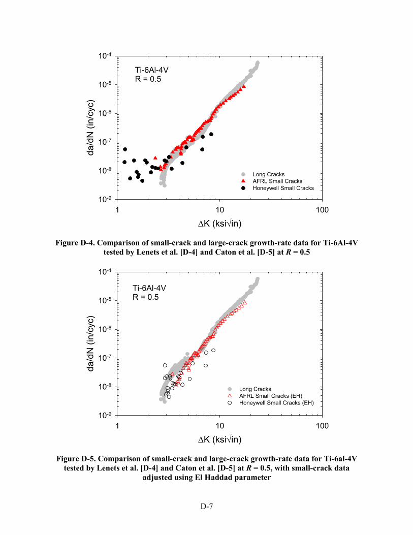
D-7

Figure D-4. Comparison of small-crack and large-crack growth-rate data for Ti-6Al-4V tested by Lenets et al. [D-4] and Caton et al. [D-5] at R = 0.5

Figure D-5. Comparison of small-crack and large-crack growth-rate data for Ti-6al-4V tested by Lenets et al. [D-4] and Caton et al. [D-5] at R = 0.5, with small-crack data

adjusted using El Haddad parameter

Ti-6Al-4VR = 0.5

K (ksiin)

1 10 100

da/d

N (

in/c

yc)

10-9

10-8

10-7

10-6

10-5

10-4

Long CracksAFRL Small CracksHoneywell Small Cracks

Ti-6Al-4VR = 0.5

K (ksiin)

1 10 100

da/d

N (

in/c

yc)

10-9

10-8

10-7

10-6

10-5

10-4

Long CracksAFRL Small Cracks (EH)Honeywell Small Cracks (EH)

D-8

Figure D-6. Comparison of small-crack and large-crack growth-rate data for Ti-6Al-4V tested by Caton et al. [D-5] at R = -1

Figure D-7. Comparison of small-crack and large-crack growth-rate data for Ti-6Al-4V tested by Caton et al. [D-5] at R = -1, with small-crack data adjusted using El Haddad

parameter

Ti-6Al-4VR = -1

K (ksiin)

1 10 100

da/d

N (

in/c

yc)

10-9

10-8

10-7

10-6

10-5

10-4

Long CracksAFRL Small Cracks

Ti-6Al-4VR = -1

K (ksiin)

1 10 100

da/d

N (

in/c

yc)

10-9

10-8

10-7

10-6

10-5

10-4

Long CracksAFRL Small Cracks (EH)

D-9

AFRL researchers also generated similar small-crack and large-crack data at room temperature for the + titanium alloy Ti-6Al-2Zr-4Sn-6Mo (Ti-6-2-4-6) [D-6]. The microstructure consisted of equiaxed primary alpha grains and lath alpha in transformed prior-beta grains, with a prior alpha area fraction around 19%. The room-temperature yield strength was approximately 165 ksi (1140 MPa). The average primary alpha grain size was approximately 3.7 m (0.00015 in.).

Small-crack tests were conducted at R = 0.05 with maximum stresses of 125 ksi, 134 ksi, or 150 ksi (860, 925, or 1040 MPa). All small cracks considered in this study were initiated naturally. A corresponding large-crack growth rate curve was available at R = 0.05. The EH small-crack parameter was estimated as a0 = 0.0008 in. (20 m) based on a large-crack threshold value of 2.55 ksiin (2.8 MPam) and an endurance limit of approximately 76 ksi (523 MPa), both at R = 0.05. Standard incremental polynomial methods with five-point windows were used to calculate da/dN.

The small-crack and large-crack data are compared without the EH correction in figure D-8 and with the EH correction in figure D-9. The differences in the two figures are not as pronounced as for the Ti-6Al-4V R = 0.1 data because the EH parameter a0 for Ti-6-2-4-6 is relatively small, but there is still a distinct small-crack effect in the uncorrected data, and the EH correction is relatively successful at matching small-crack and large-crack data.

Note that the EH parameter a0 is smaller for the Ti-6-2-4-6 than for the Ti-6Al-4V, consistent with the smaller primary alpha grain size for the Ti-6-2-4-6. In both cases, a0 is approximately 5.4 times larger than the primary alpha grain size.

Figure D-8. Comparison of small-crack and large-crack growth-rate data for Ti-6Al-2Zr-4Sn-6Mo tested by Jha et al. [D-6] at R = 0.05

Ti-6Al-2Sn-4Zr-6MoR = 0.05

K (ksiin)

1 10 100

da/d

N (

in/c

yc)

10-9

10-8

10-7

10-6

10-5

10-4

AFRL Small CracksLong Cracks

D-10

Figure D-9. Comparison of small-crack and large-crack growth rate data for Ti-6Al-2Zr-4Sn-6Mo tested by Jha et al. [D-6] at R = 0.05, with small-crack data adjusted using

El Haddad parameter

Additional small-crack data for Ti-6Al-4V were available in the literature. Brown and Taylor [D-9] published room-temperature small-crack and large-crack data for Ti-6Al-4V in two different microstructural forms. One form was a standard mill-annealed microstructure with equiaxed alpha and intergranular beta. A slightly coarser grain structure with the same general phase characteristics was obtained through additional heat treating. The corresponding average grain sizes were quoted as being 4.7 m (0.00019 in.) and 11.7 m (0.00046 in.), respectively. The tensile yield strength was cited as 900 MPa (130 ksi) without specifically referencing either one of the microstructural forms. Small-crack tests were performed with 10 mm square bars in four-point bending at R = 0.2 with a maximum stress of 750 MPa (109 ksi). Crack growth was monitored with plastic replication. The original experimental data were not available, but instead the graphs of da/dN versus K were digitized from the published paper. Because the K relationship used in their study was given in the paper, it was possible to back-calculate the corresponding crack sizes. Brown and Taylor also cited values for the large crack threshold (5 MPam) and the smooth specimen endurance limit (500 MPa), again without specific reference to either specific microstructural form. This gives an EH parameter a0 = 69 m (0.0027 in.).

Comparisons of the small-crack and large-crack data for the coarse-grained and fine-grained microstructures are shown in figures D-10 and D-11, respectively. Each graph shows both the uncorrected small-crack data as well as the small-crack data adjusted with the EH model using the EH parameter cited by Brown and Taylor. The correlation is reasonably successful for the coarse grained material but slightly nonconservative for the fine-grained material; the adjusted small-crack growth rates are still somewhat higher than the large-crack growth-rate trends.

Ti-6Al-2Sn-4Zr-6MoR = 0.05

K (ksiin)

1 10 100

da/d

N (

in/c

yc)

10-9

10-8

10-7

10-6

10-5

10-4

AFRL Small Cracks (EH)Long Cracks

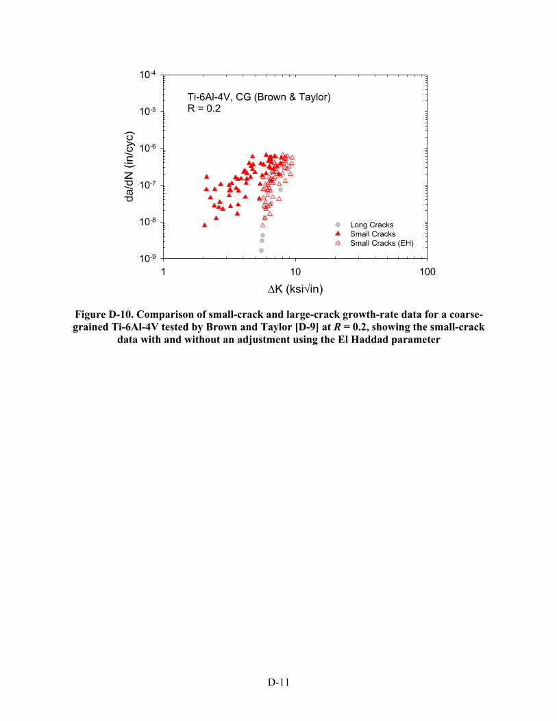
D-11

Figure D-10. Comparison of small-crack and large-crack growth-rate data for a coarse-grained Ti-6Al-4V tested by Brown and Taylor [D-9] at R = 0.2, showing the small-crack

data with and without an adjustment using the El Haddad parameter

Ti-6Al-4V, CG (Brown & Taylor)R = 0.2

K (ksiin)

1 10 100

da/d

N (

in/c

yc)

10-9

10-8

10-7

10-6

10-5

10-4

Long CracksSmall CracksSmall Cracks (EH)

D-12

Figure D-11. Comparison of small-crack and large-crack growth-rate data for a fine-grained Ti-6Al-4V, tested by Brown and Taylor [D-9] at R = 0.2, showing the small-crack

data with and without an adjustment using the El Haddad parameter

Hicks and Brown [D-10] have also published room-temperature small-crack and large-crack data for an IMI 685 titanium alloy with a much larger grain size cited: 3500 m (0.138 in.). Unfortunately, no further information was provided about the microstructure. The yield strength was cited as 780 MPa (113 ksi) and the ultimate tensile strength as 800 MPa (116 ksi). The small-crack tests were conducted on 10 mm square bars in four-point bending at R = 0.1. The original experimental data were not available, so the graphs of da/dN versus K were again digitized to extract the data. The specific maximum stresses were not given in the paper, but they were cited as always being between 80% and 100% of the yield strength. To back-calculate the crack sizes to apply the EH correction, it was assumed that the maximum stress was 90% of the yield strength. By maintaining consistency in both forward and reverse calculations, the potential 10% error in this assumption should have only a minor impact on the overall correlations.

Although large-crack threshold values were evident from the published graphs, Hicks and Brown did not cite an endurance limit, so it was not possible to calculate the EH parameter in the usual way. However, it had previously been noted from analysis of the AFRL Ti-6Al-4V and Ti-6-2-4-6 that a0 scaled with the grain size (approximately 5.4 times larger). In the Brown and Taylor data, the cited a0 was either 5.9 times the cited grain size (for the coarse-grained material) or 15 times the cited grain size (for the fine-grained material). Therefore, it seemed reasonable to assume for the Hicks and Brown data that the unknown EH parameter a0 might also scale with the cited grain size. Choosing a factor of 6 gives an estimated EH parameter a0 = 21 mm (0.826 in.). Unfortunately, this is an absurdly large number, and leads to a completely unsuccessful correlation of the small-crack and large-crack data. See figure D-12. Also included in figure D-12 is a completely empirical selection of an a0 value that approximately lines up the small-crack and large-

Ti-6Al-4V, FG (Brown & Taylor)R = 0.2

K (ksiin)

1 10 100

da/d

N (

in/c

yc)

10-9

10-8

10-7

10-6

10-5

10-4

Long CracksSmall CracksSmall Cracks (EH)

D-13

crack data. This value of a0 was found to be approximately 1.4 mm—still an extremely large value—but over an order of magnitude smaller than the value calculated from the original microstructural scaling. IMI 685 has a Widmanstatten alpha + beta colony structure with a large prior beta grain size, and so the relevant microstructural dimension for this microstructure is probably the colony size instead of the grain size. The Widmanstatten (or lamellar) α + β microstructure is also conducive to crack deflection and roughness-induced crack closure. The large Kth shown in figure D-12 is likely the result of roughness-induced crack closure. If the Kth

was corrected for the effects of crack closure, the a0 value would be reduced, and the agreement with experimental data would likely be improved.

Hicks and Brown [D-10] also showed small-crack and large-crack data for IMI 318, which is the same as Ti-6Al-4V. However, these data had a strong resemblance to the fine-grained Ti-6Al-4V data published in reference [D-9] (see again figure D-11), and because the two papers share a common author, it is likely that they are in fact derived from the same test data, despite some test conditions being reported differently in the two papers.

Figure D-12. Comparison of small-crack and large-crack growth-rate data for IMI 685 tested by Hicks and Brown [D-10] at R = 0.1, showing the small-crack data with and

without an adjustment, using various estimates of the El Haddad parameter

D.5.2 NICKEL-BASED SUPERALLOYS

Jha et al. [D-7] at AFRL performed large-crack and small-crack tests at 650C (1200F) with the nickel-based superalloy IN-100. The material was fine-grained, subsolvus, and powder-processed with a median -grain size approximately 4 m (0.00016 in.). The yield strength at the test

IMI 685 (Hicks & Brown)R = 0.1

K (ksiin)

1 10 100

da/d

N (

in/c

yc)

10-9

10-8

10-7

10-6

10-5

10-4

Long CracksSmall CracksSmall Cracks (EH)Small Cracks (EH empirical)

D-14

temperature was approximately 1100 MPa (160 ksi), the UTS was approximately 1379 MPa (200 ksi), and the % elongation at fracture was approximately 20%.

Small-crack tests were performed at R = 0.05 using mostly cylindrical smooth specimens under uniform tension (one test was conducted with a square bar under bending). Tests were conducted at two different maximum stress values: 1150 MPa (167 ksi) and 1200 MPa (174 ksi). Note that both of these values are greater than the yield strength. Test frequency was 0.33 Hz. Some cracks originated naturally at nonmetallic particles on the surface, whereas other cracks initiated naturally at surface pores. Crack-length measurements were performed with acetate replicas at room temperature during interruptions in the test. The original a versus N data were provided to SwRI for analysis following the protocols of this study. The Forman-Shivakumar solution was used here to calculate K, and second-order polynomial methods with sliding three-point windows were used to calculate da/dN (the secant method was used for one small dataset). Large crack da/dN versus K data generated with C(T) specimens were also provided to SwRI.

Comparisons of the large-crack and small-crack data are shown in figure D-13. Note that the small-crack tests at 1200 MPa exhibited noticeably faster growth rates than the tests at 1150 MPa.

Figure D-13. Comparison of small-crack and large-crack growth-rate data for IN-100, tested by Jha et al. [D-7] at R = 0.05

This difference is not accommodated by linear elastic fracture mechanics (LEFM) approaches based on K, and may arise from the very large maximum stresses (above yield). Also note that the single set of data for a crack originating at a nonmetallic particle exhibited noticeably faster growth rates than the five sets of data for cracks originating at pores at the same stress level; again, this distinction is not accommodated by the simple linear-elastic fracture mechanics approach used here.

IN100 (AFRL)R = 0.05

K (ksiin)

1 10 100

da/d

N (

in/c

yc)

10-9

10-8

10-7

10-6

10-5

10-4

167 ksi (Pore)167 ksi (NMP)174 ksi (Pore)Long Cracks

D-15

Two approaches were used to estimate the EH parameter, one from equation D-1 and one by scaling the grain size. The large-crack threshold was measured to be 12.3 MPam from a single reported large-crack test. Estimating the endurance limit was difficult because smooth-specimen fatigue tests (R = 0.05) were conducted only at maximum stresses of 1000 MPa, 1100 MPa, 1150 MPa, and 1200 MPa. At the lowest stress level tested, failures were observed at lives ranging from 60,000 cycles to nearly 1,000,000 cycles. The earlier failures were mostly associated with crack initiation at subsurface nonmetallic particles. The longer lives (300,000 to 950,000 cycles) were mostly associated with crack initiation at surface pores, which is thought to be more relevant to the EH estimate. Based on extrapolation of the available failure data for surface pore cracks, the endurance limit was crudely estimated to be approximately σe = 900 MPa. This estimate and the measured large-crack threshold led to an estimated EH parameter a0 = 132 m (0.0052 in.). An alternative value was calculated by scaling the median -grain size: six times this dimension (the value derived from the titanium alloy studies) is 24 m (approximately 0.001 in.).

Comparisons of large-crack data and EH-corrected small-crack data are shown in figure D-14. The EH estimate based on equation D-1 overpredicted the small-crack effect (compared to the available large-crack data). The EH estimate based on scaling the median -grain size slightly under-predicted the small-crack effect for some data points, while successfully predicting it elsewhere.

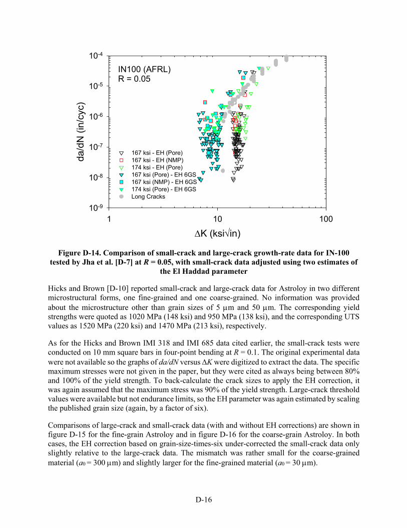
D-16

Figure D-14. Comparison of small-crack and large-crack growth-rate data for IN-100 tested by Jha et al. [D-7] at R = 0.05, with small-crack data adjusted using two estimates of

the El Haddad parameter

Hicks and Brown [D-10] reported small-crack and large-crack data for Astroloy in two different microstructural forms, one fine-grained and one coarse-grained. No information was provided about the microstructure other than grain sizes of 5 m and 50 m. The corresponding yield strengths were quoted as 1020 MPa (148 ksi) and 950 MPa (138 ksi), and the corresponding UTS values as 1520 MPa (220 ksi) and 1470 MPa (213 ksi), respectively.

As for the Hicks and Brown IMI 318 and IMI 685 data cited earlier, the small-crack tests were conducted on 10 mm square bars in four-point bending at R = 0.1. The original experimental data were not available so the graphs of da/dN versus K were digitized to extract the data. The specific maximum stresses were not given in the paper, but they were cited as always being between 80% and 100% of the yield strength. To back-calculate the crack sizes to apply the EH correction, it was again assumed that the maximum stress was 90% of the yield strength. Large-crack threshold values were available but not endurance limits, so the EH parameter was again estimated by scaling the published grain size (again, by a factor of six).

Comparisons of large-crack and small-crack data (with and without EH corrections) are shown in figure D-15 for the fine-grain Astroloy and in figure D-16 for the coarse-grain Astroloy. In both cases, the EH correction based on grain-size-times-six under-corrected the small-crack data only slightly relative to the large-crack data. The mismatch was rather small for the coarse-grained material (a0 = 300 m) and slightly larger for the fine-grained material (a0 = 30 m).

IN100 (AFRL)R = 0.05

K (ksiin)

1 10 100

da/d

N (

in/c

yc)

10-9

10-8

10-7

10-6

10-5

10-4

167 ksi - EH (Pore)167 ksi - EH (NMP)174 ksi - EH (Pore)167 ksi (Pore) - EH 6GS167 ksi (NMP) - EH 6GS174 ksi (Pore) - EH 6GSLong Cracks

D-17

Figure D-15. Comparison of small-crack and large-crack growth-rate data for a fine-grain Astroloy reported by Hicks and Brown [D-10] at R = 0.1, showing the small-crack data

with and without an adjustment using an estimated El Haddad parameter

Figure D-16. Comparison of small-crack and large-crack growth-rate data for a coarse-grain Astroloy reported by Hicks and Brown [D-10] at R = 0.1, showing the small-crack

data with and without an adjustment using an estimated El Haddad parameter

FG AstroloyR = 0.1

K (ksiin)

1 10 100

da/d

N (

in/c

yc)

10-9

10-8

10-7

10-6

10-5

10-4

Small CracksSmall Cracks (EH)Long Cracks

CG AstroloyR = 0.1

K (ksiin)

1 10 100

da/d

N (

in/c

yc)

10-9

10-8

10-7

10-6

10-5

10-4

Small CracksSmall Cracks (EH)Long Cracks

D-18

Kantzos, Telesman, and colleagues at NASA Glenn Research Center have performed extensive research on the nickel-based powder metallurgy alloy Udimet 720 (U720) [D-8]. Powder was consolidated using typical disk alloy processing: hot isostatic pressing followed by extrusion, then isothermal forging into pancakes. All forgings were given a subsolvus solution heat treatment, followed by an oil quench and aging treatment. The resulting microstructure had a typical grain size ASTM 11 (average grain diameter was approximately 8 m).

Small-crack tests were performed at 1200F (650C) on cylindrical, axially loaded fatigue specimens with a 0.40-inch (10.2 mm) diameter. All cracks were initiated naturally at artificially seeded ceramic inclusions with average seed diameters of 0.0021 in. (54 m) or 0.0048 in. (122 m). Crack-size measurements were performed in a special rotational stage in a scanning electron microscope. Fatigue cycling at 20 CPM in ambient laboratory air was periodically interrupted and the specimen transferred to the SEM stage to map and track SC growth. The fatigue cycling was initially performed under strain control at 20 CPM (0.33 Hz) with strain ratios of R = 0 or -1 under strain ranges of 0.6% or 0.8%. Following an initial cycling period during which maximum and minimum loads stabilized, testing continued to failure under load control at a frequency of 5 Hz. The corresponding small-crack load ratios were approximately R = -0.33 or R = -1. The maximum stresses in the small crack tests varied from 154 ksi (1062 MPa) to 163 ksi (1124 MPa) for R = -0.33 and from 107 ksi (737 MPa) to 109 ksi (752 MPa) for R = -1. Telesman provided an extensive database of small-crack results, and only a portion of these tests were selected for detailed examination in this study. Furthermore, data from the first 250 cycles of fatigue testing (the so-called pop-in period) were excluded from the study. Large-crack tests were performed for comparison under load control at 1200F with so-called Kb bar (SC) specimens at R = -0.25 or -1.

Comparisons of large-crack and small-crack data (with and without EH corrections) are shown in figures D-17 and D-18 for R = -0.33 and figures D-19 and D-20 for R = -1. Because endurance limit data were not available, the EH parameter was again estimated by scaling the published grain size by a factor of six. The EH correction was successful in correlating large-crack and small-crack data at R = -0.33. At R = -1, the EH correction undercorrected the small-crack data relative to the large-crack data, although it did successfully consolidate the small-crack data. Unfortunately, only near-threshold small-crack data were available.

D-19

Figure D-17. Comparison of small-crack and large-crack growth-rate data for U720 tested by Kantzos et al. [D-8] at R = -0.33

Figure D-18. Comparison of small-crack and large-crack growth-rate data for U720 tested by Kantzos et al. [D-8] at R = -0.33, with small-crack data adjusted using El Haddad

parameter

U720 (NASA)R = -0.33 (Strain Control R

K (ksiin)

1 10 100

da

/dN

(in

/cyc

)

10-9

10-8

10-7

10-6

10-5

10-4

Long Cracks (R = -0.25)Small Cracks

U720 (NASA)R = -0.33 (Strain Control R

K (ksiin)

1 10 100

da

/dN

(in

/cyc

)

10-9

10-8

10-7

10-6

10-5

10-4

Long Cracks (R = -0.25)Small Cracks (EH)

D-20

Figure D-19. Comparison of small-crack and large-crack growth-rate data for U720, tested by Kantzos et al. [D-8] at R = -1

Figure D-20. Comparison of small-crack and large-crack growth-rate data for U720 tested by Kantzos et al. [D-8] at R = -1, with small-crack data adjusted using El Haddad

parameter

U720 (NASA)R = -1.0 (Strain Control R

K (ksiin)

1 10 100

da

/dN

(in

/cyc

)

10-9

10-8

10-7

10-6

10-5

10-4

Long Cracks (R = -1.0)Small Cracks

U720 (NASA)R = -1.0 (Strain Control R

K (ksiin)

1 10 100

da

/dN

(in

/cyc

)

10-9

10-8

10-7

10-6

10-5

10-4

Long Cracks (R = -1.0)Small Cracks (EH)

D-21

D.6 DISCUSSION

The data evaluated in this study all indicate that common aircraft gas turbine engine rotor alloys typically exhibit accelerated growth rates when crack sizes are very small and that these growth rates tend to merge with large-crack trends as the cracks become larger. A simple model originally proposed by El Haddad in which a small-crack length parameter is added to the physical crack size before calculating the SIF was shown to be reasonably successful in correlating small-crack and large-crack growth-rate data for several different rotor materials. The data evaluated included multiple titanium and nickel-based alloys at different stress ratios and temperatures. In some cases, the El Haddad length parameter could not be calculated directly from threshold and endurance limit values because these were not available, but simple estimates of the EH parameter scaled to the grain size were reasonably successful in correlating large-crack and small-crack data in most cases.

D.6.1 LIMITATIONS AND DIFFICULTIES

Some of the “bounds” of this study (stated at the outset) should be reviewed to emphasize the limited scope of these observations and conclusions. Microstructurally small cracks (cracks on the order of the grain size or smaller) were avoided in most cases, and as a result, crack arrest phenomena (and the complications they introduce) were pushed more into the background. Significant plasticity was also avoided to the extent possible. Staying within these two boundaries generally means that linear elastic fracture mechanics (and, therefore, K) should be approximately valid (this would not be true for microstructurally small cracks or elastic-plastic loading conditions).

There are several practical difficulties associated with the El Haddad approach when a0 is estimated from equation D-1. For example, it is sometimes difficult to define an endurance limit for some materials. Studies during the last two decades in the high-cycle-fatigue and very-high-cycle-fatigue regimes have indicated that many materials do not exhibit a distinct plateau in fatigue strength at very long lives but that the fatigue strength may continue to decrease with further cycling. A stated endurance limit may merely reflect the limits imposed on fatigue-test duration. A shorter test duration may lead to an overestimate of the endurance limit, which will give an underestimate of the EH parameter and potentially an underestimate of small-crack growth rates.

In addition, it is sometimes observed that the failure mode for smooth specimen fatigue tests may shift from surface initiation to subsurface initiation at very long lifetimes. Because equation D-1 requires some assumption about the crack geometry of interest, a shift from an SC to an embedded crack will require a change in the formulation (and may introduce a discontinuity or conflict between data derived from different failure modes). Equation D-1 is applicable only to endurance limits associated with surface failure modes. The failure origins associated with high-cycle-fatigue specimens are not always reported. If the endurance limit for SC behavior is estimated to be too low because it is influenced by subsurface failures at longer lives, then the EH parameter may be estimated to be too large, thereby overestimating small-crack growth rates.

Furthermore, fatigue-failure behavior in some materials may be controlled by populations of inclusions, and the life-limiting crack in a specimen may be associated with a particularly large defect. Any effect of this defect on the growth (or nongrowth) of microcracks (associated, for

D-22

example, with local stress concentrations or residual stresses) is not reflected in the formulation behind equation D-1. In some cases, the defect may be sufficiently large that the initial resulting microcrack is larger than a0, thereby raising additional questions about the formulation. If the intended goal of the EH small-crack formulation is to describe crack-growth behavior in normal matrix material, then properties derived from defect-dominated behavior may be inappropriate. However, if the cracks of interest in the material always arise from such defects, then the formulation may end up being self-consistent.

A different set of difficulties is associated with characterization of the large-crack threshold, the other key input into equation D-1. It is now known that the apparent large-crack threshold can be influenced both by test technique (e.g., traditional load-shedding methods) and specimen geometry (large-crack thresholds generated with C(T) specimens are sometimes observed to be higher than with middle-crack tension (M(T)) specimens). The most common error appears to be an overestimation of Kth based on C(T) tests at R 0 using traditional load-shed methods. Underestimation of Kth appears to be less likely. An overestimate of Kth will contribute to an overestimate of a0 and an overestimate of small-crack growth rates.

Another complication associated with the large-crack threshold is that other environmental factors may influence the apparent value of this threshold (for example, if corrosion product builds up on the crack faces and causes premature arrest due to oxide-induced crack closure). There may also be environmental influences on small SCs in service, but there may not be adequate similitude between the threshold test configuration and the small-crack configuration for the threshold data to be transferable to the EH calculation. Again, an overestimate of Kth would lead to an overestimate of small-crack growth rates by the EH model.

Given these difficulties associated with obtaining appropriate input data to estimate the EH parameter, it is encouraging that some success was observed using microstructurally motivated estimates of a0. It may also be practical to use totally empirical estimates of a0 in some cases, as was also done here in a few cases. However, the more empirical the estimate, the greater the need for adequate small-crack growth-rate data to validate the estimate.

There is no shortage of more sophisticated small-crack growth-rate models in the literature; many are micromechanical models that incorporate the effects of microstructural barriers, local plasticity, crack closure, and other factors. It may be warranted to investigate one or more of these alternative models in subsequent investigations, given the imperfection of the El Haddad model. However, models with more sophistication also introduce more complexity and more need for data to feed them—data which are often not available in traditional industrial material databases. One of the great attractions of the EH model is its simplicity; it is easily fed by existing data or is easily calibrated.

The physical meaning of the EH length parameter also deserves some further discussion. El Haddad originally considered a0 to be an intrinsic crack length in the microstructure. Such an interpretation is troublesome, however, because a0 is on the order of several grain diameters. The FCG threshold value for small cracks is known to increase with crack length, approaching the long-crack value when the crack becomes large. A more reasonable and physically appealing interpretation for a0 is simply that it describes the length scale at which the FCG threshold of the small crack approaches that of the large-crack threshold.

D-23

All data cited in this brief study are based on cracks growing under uniform tension or slight bending gradients. In component applications, small cracks are likely to form in regions with pronounced stress gradients. The applicability of the EH approach to such cracks has not been studied rigorously, but the first author has found some success using these approaches in unpublished research to predict the FCG lifetimes of cracks growing in residual stress fields from shot peening or other surface enhancement methods.

Finally, this brief study has not considered time-dependent effects, such as dwell periods. Jha et al. [7] showed a few IN-100 datasets for large-crack and small-crack behavior with 6-sec dwell periods. The dwell caused little or no change in the large-crack growth rates (possibly a small increase in the threshold value) but a significant change in the small-crack growth rates (a substantial increase). The EH approach would not capture this behavior. However, it is possible that the dwell effect in the small-crack data was affected by the significantly higher maximum stresses in the small-crack tests—higher than the yield strength. Clearly, further work is needed to sort out time-dependent effects on small crack growth rate behaviors and models.

D.6.2 SIGNIFICANCE OF SMALL-CRACK EFFECTS FOR ROTOR APPLICATIONS

Are these small-crack growth rate effects actually significant for life management of aircraft engine rotors in real-world applications? To explore this question, a series of simple analytical studies were performed. The model material was the Ti-6Al-4V alloy from the HCF program cited previously. Crack-growth life predictions were performed for constant amplitude, R = 0.1 stress cycling of a semi-elliptical SC in a semi-infinite plate. The predictions were performed using both conventional large-crack models and the El Haddad small-crack model discussed in this paper (with a0 = 0.0021 in.). In particular, the SIF calculation for the small-crack prediction was modified in accordance with equation D-2. The fracture toughness was assumed to be 60 ksi√in. Predictions were performed for a variety of initial crack sizes, ranging from crack depth a = 0.001 in. to a = 0.015 in., and a variety of stress amplitudes, with maximum applied stresses approaching the cyclic yield strength. The calculations were performed in a special version of DARWIN (with the modified stress-intensity factor expression).

To ensure that the representation of the large-crack data did not unduly influence the results, two different forms were used. The first was a simple tabular representation of the available large-crack data at R = 0.1. The second was a fit of these data to the standard NASGRO 4.0 equation (hereafter denoted as simply the NASGRO equation), assuming a typical value of α = 2.5 for the constraint factor. The small-crack correction term in the NASGRO threshold expression was turned off for these calculations, as explained below. The original tabular data and the NASGRO fit are shown in figure D-21. The two representations had slightly different values of the large-crack threshold. The tabular representation assumed that the lowest ΔK value in the table, 4 ksi√in, was the threshold value. To ensure that the NASGRO fit passed reasonably close to this particular point, it was necessary to specify a slightly lower value of the threshold asymptote, approximately 3.89 ksi√in.

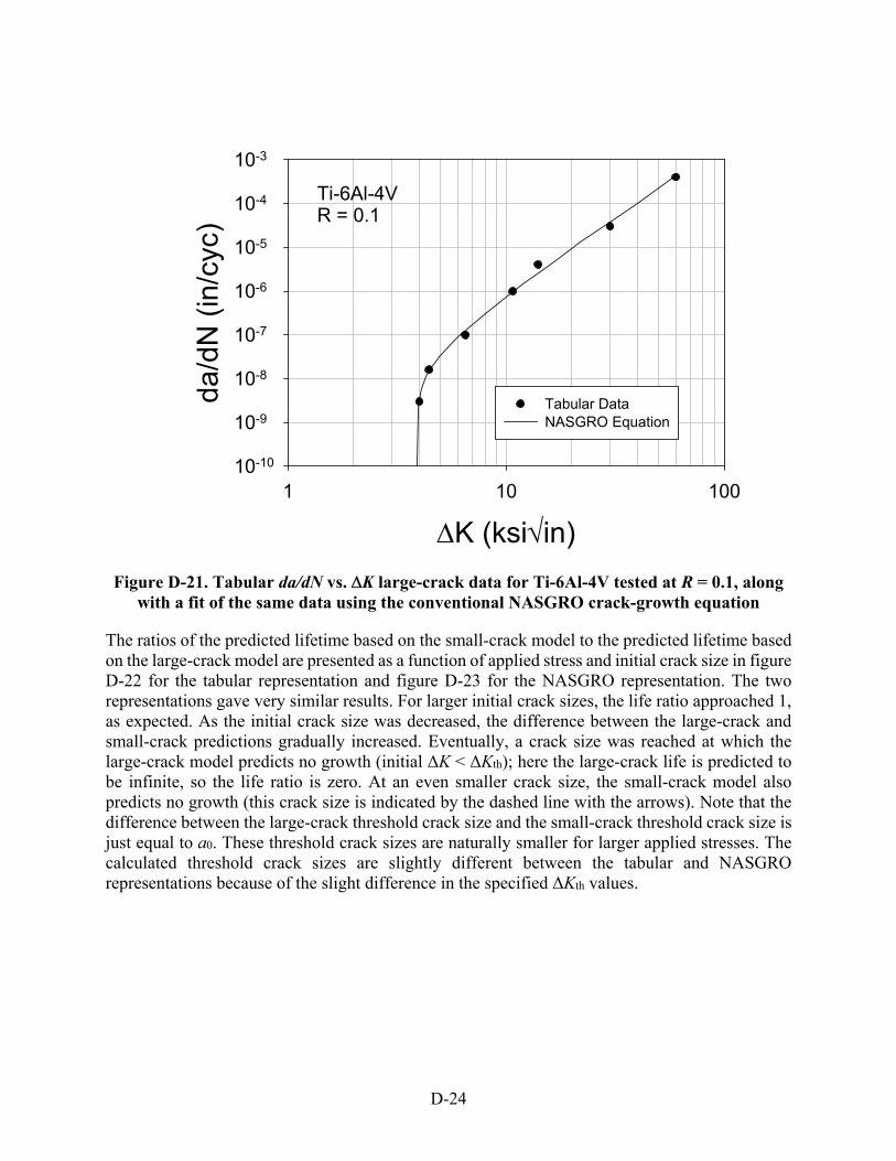
D-24

Figure D-21. Tabular da/dN vs. K large-crack data for Ti-6Al-4V tested at R = 0.1, along with a fit of the same data using the conventional NASGRO crack-growth equation

The ratios of the predicted lifetime based on the small-crack model to the predicted lifetime based on the large-crack model are presented as a function of applied stress and initial crack size in figure D-22 for the tabular representation and figure D-23 for the NASGRO representation. The two representations gave very similar results. For larger initial crack sizes, the life ratio approached 1, as expected. As the initial crack size was decreased, the difference between the large-crack and small-crack predictions gradually increased. Eventually, a crack size was reached at which the large-crack model predicts no growth (initial ΔK < ΔKth); here the large-crack life is predicted to be infinite, so the life ratio is zero. At an even smaller crack size, the small-crack model also predicts no growth (this crack size is indicated by the dashed line with the arrows). Note that the difference between the large-crack threshold crack size and the small-crack threshold crack size is just equal to a0. These threshold crack sizes are naturally smaller for larger applied stresses. The calculated threshold crack sizes are slightly different between the tabular and NASGRO representations because of the slight difference in the specified ΔKth values.

K (ksiin)

1 10 100

da/d

N (

in/c

yc)

10-10

10-9

10-8

10-7

10-6

10-5

10-4

10-3

Tabular Data NASGRO Equation

Ti-6Al-4VR = 0.1

D-25

Figure D-22. Predicted life ratios for small-crack vs. large-crack models assuming tabular da/dN vs. K large-crack data and a small-crack model with a0 in the SIF term

Figure D-23. Predicted life ratios for small-crack vs. large-crack models assuming a NASGRO crack growth equation and a small-crack model with a0 in the SIF term

Initial crack depth, a (inches)

0.000 0.002 0.004 0.006 0.008 0.010 0.012 0.014

Nsm

all c

rack

/Nla

rge

crac

k

0.0

0.2

0.4

0.6

0.8

1.0

= 36 ksi = 45 ksi = 54 ksi = 72 ksi= 90 ksi = 108 ksi

Tabular data with a0 in stress intensity factor

Initial crack depth, a (inches)

0.000 0.002 0.004 0.006 0.008 0.010 0.012 0.014

Nsm

all c

rack

/Nla

rge

crac

k

0.0

0.2

0.4

0.6

0.8

1.0

= 36 ksi = 45 ksi = 54 ksi = 72 ksi = 90 ksi = 108 ksi

NASGRO Equation with a0

in stress intensity factor

D-26

The NASGRO equation itself contains a potential small-crack adjustment in the threshold term. This equation is given by:

(D-3)

Where the threshold parameter ΔKth is described for R > 0 by the form:

(D-4)

With:

(D-5)

Here K1 is conceptually the value of the large-crack threshold as R 1.0. The parameter Cpth is

a “fanning” factor that describes spreading of the da/dN curves with changing R near threshold; the function f in both equations D-3 and D-4 is the Newman crack closure equation [D-22]; and A0 is a term in the Newman equation.

This is an alternative interpretation of the El Haddad model that applies the correction to the material resistance (SIF threshold) term instead of the driving force (applied SIF) term. As such, the small-crack correction should NOT be implemented in both terms simultaneously. Therefore, in the earlier calculations in the present study where a0 was applied to the driving force term, the other “a0” value in the NASGRO threshold expression was set equal to zero.

However, the reverse implementation is also possible: set a0 equal to zero in the driving force term, and use the nonzero a0 value in the threshold term. This is the conventional use of the NASGRO equation (e.g., in the NASGRO software itself). This implementation was explored with a similar analytical study, and the results are shown in figure D-24. The overall trends are the same, and the limiting values at small crack sizes are the same, but the curve shapes are slightly different. Here the ratio of the small-crack and large-crack models approaches 1.0 more quickly and drops off to 0 more sharply with decreasing initial crack size as the large-crack threshold is approached. Essentially, the small-crack effect is slightly less pronounced, except for conditions near or below the large-crack threshold. However, in that regime, the small-crack effect is still strong.

da

dNC

f

RK

KK

KK

nth

p

c

q

1

1

1

1

max

pth

pth

CR

RC

th ARf

RKK )1(

0

)1(

*1 )1/(

][1

1

2/1

01

*1

aa

aKK

D-27

Figure D-24. Predicted life ratios for small-crack vs. large-crack models, assuming a NASGRO crack growth equation and a small-crack model with a0 in the threshold term

The strong similarity between figures D-23 and D-24, which use different formulations of the EH approach, invite a further comparison of the performance of these two formulations. Figure D-25 shows the ratio of the predicted FCG lifetimes using the two small-crack model formulations (a0 appearing in the material resistance [threshold] term or the driving force [applied SIF] term). The results indicate that the differences in the two approaches are relatively inconsequential for life prediction (factors close to 1), except at the smallest initial crack sizes (which are significant only for larger applied cyclic stresses). The differences can be more significant (factors of 2 on life) for initial crack sizes on the order of a0. All these conclusions apply to the specific demonstration problems considered, and their generality to other problems cannot automatically be assumed.

There may be other practical considerations involved in deciding whether to represent the small-crack effect in the threshold term or the applied SIF term. It is relatively simple to alter the value of ΔKth in the NASGRO equation formulation, which does not require changes in other equation parameters to preserve the fit quality elsewhere. However, some other crack-growth equations have threshold terms that are highly correlated to other terms in the equations, and so a change in the threshold value may disrupt the fit elsewhere. Therefore, it may be more robust to implement the small-crack effect in the driving force term for implementation with different representations of material resistance.

Initial crack depth, a (inches)

0.000 0.002 0.004 0.006 0.008 0.010 0.012 0.014

Nsm

all c

rack

/Nla

rge

crac

k

0.0

0.2

0.4

0.6

0.8

1.0

= 36 ksi = 45 ksi = 54 ksi = 72 ksi = 90 ksi = 108 ksi

NASGRO Equation with a0

in threshold term

D-28

Figure D-25. Ratio of predicted lifetimes using small-crack models in which a0 appears in either the threshold term or the driving force term

Van Stone [D-23,D-24] has reported results for experiments involving small cracks in René 95 in which lifetimes were satisfactorily predicted using large-crack data and methods (i.e., no small-crack effect was observed). However, a closer look at those data in the perspective of the current model suggests that a significant small-crack effect would probably not have been expected. Insufficient data were available to calculate a0 directly, but the cited grain size of René 95 was approximately 0.0002 inches (5 microns). Estimating a0 as six times the grain size (a method that was shown to be useful earlier in this study) gives a value of a0 = 0.0012 inches (0.030 mm). The smallest initial crack sizes employed by Van Stone were ai = 0.0025 inches, and other small-crack tests started with initial crack sizes as large as 0.010 inches. Therefore, all tests started with cracks significantly larger than a0. Furthermore, all tests were conducted at reasonably large maximum stress values—100 to 130 ksi (689 to 896 MPa). Although insufficient René 95 data and insufficient information about the specific tests conducted were available to construct diagrams similar to figures D-22–D-24, the earlier numerical studies suggest that, when maximum stresses are large and when initial crack sizes are significantly larger than a0, only small changes in life (10% to 30%) are expected. These subtle differences are smaller than the typical test-to-test life scatter for the data reported by Van Stone at all initial crack depths (including large cracks).

Furthermore, the small cracks tested by Van Stone were not actually naturally occurring small cracks. They were large cracks that had been grown from an electro-discharged machined (EDM) notch, and then the EDM notch had been machined away to reduce the crack size. This particular test method, although practiced occasionally in the early days of small-crack research, has now

Initial crack depth, a (inches)

0.000 0.002 0.004 0.006 0.008 0.010 0.012 0.014Nsm

all c

rack

(th

resh

)/N

sma

ll cr

ack

(S

IF)

1.0

1.2

1.4

1.6

1.8

2.0

2.2

2.4

2.6

2.8

3.0

3.2

= 36 ksi = 45 ksi = 54 ksi = 72 ksi = 90 ksi = 108 ksi

NASGRO Equation, life ratio with a0 in threshold

or a0 in stress intensity factor

D-29

fallen out of favor because researchers have realized that cracks formed in this manner do not necessarily exhibit the same growth rate characteristics as natural small cracks. All the small crack data evaluated earlier in the present study were generated from natural small cracks or were formed at extremely small FIB notches (without any subsequent machining).

Therefore, the Van Stone results do not appear to contradict the present study. Nevertheless, the Van Stone study does demonstrate that small-crack effects may not be significant for some practical applications because of the particular combinations of material microstructure, initial crack size, and applied stress. In particular, when microstructures have very fine grain sizes and when applied stresses are large, crack sizes may have to be extremely small to exhibit a “small-crack” growth rate effect.

The hypothetical results described in figures D-22–D-24 have an interesting implication for conventional damage-tolerance analysis. It is common in gas-turbine-engine life management to calculate the FCG life starting from a semicircular SC with initial depth = 0.015 in. (0.38 mm). The small-crack model that includes a0 in the driving force term (figures D-22 and D-23) implies that ignoring small-crack effects for an initial crack depth of 0.015 inches will result in a life-prediction error of approximately 10% (for the specific material and loading conditions considered). This is a very small error, especially in comparison to customary scatter in lifetime results, but it is a systematic bias in the nonconservative direction. The NASGRO model with a0 in the threshold term (figure D-24) implies that this bias will be almost negligible for an initial crack size of 0.015 inches.

D.6.3 POTENTIAL ISSUES WITH LARGE-CRACK TEST RESULTS NEAR THRESHOLD

One of the longstanding controversies in studies of small fatigue cracks has been whether the small-crack behavior is anomalous or if it is actually the large-crack behavior near threshold that is anomalous. Newman [D-25–D-27], in particular, has raised concerns about load-history effects introduced by common test techniques for generation of near-threshold FCG data. The most commonly used threshold test technique [D-28] involves gradual shedding of load amplitude as the applied SIF decreases to approach the threshold value and the crack-growth rate significantly decreases. Therefore, it has been argued that the effect of the load history on crack closure could artificially reduce the near-threshold crack-growth rate.

Newman has been actively promoting alternative test techniques for large-crack near-threshold testing in an attempt to avoid the anomalous load-history effects in the conventional load-reduction (LR) test method. One such method (compression-precracking, constant amplitude, or CPCA) involves precracking of a compact-tension specimen under a compression-compression load history until the crack arrests naturally, followed by constant amplitude loading at the desired load ratio. Another method employs compression-precracking followed by a load reduction process (CPLR) that starts at a significant smaller initial value of ΔK. Newman has shown that for some materials, CPCA and CPLR methods can give significantly different threshold values than traditional LR methods.

One of the materials that Newman has studied is the same HCF program Ti-6Al-4V alloy cited earlier in this report, for which extensive large-crack and small-crack data are available.

D-30

This coincidence permits a direct comparison, therefore, of small-crack data against large-crack data in which it is thought that potentially anomalous LR threshold behavior has been eliminated.

Figure D-26 compares the Newman et al. [D-27] CPCA large-crack data against the previously cited small-crack data from Lenets et al. [D-3, D-4] and Caton et al. [D-5], as well as the previously cited large-crack data [19, 20]. Near-threshold data in these latter large-crack tests were all generated using LR methods. All of these data are at R = 0.1. The data show that although there is, in fact, a small difference between the CPCA and conventional long crack data in the near-threshold regime, the small cracks exhibit growth rates considerably higher than the CPCA data. Furthermore, the small cracks can grow at ΔK values significantly lower than the apparent ΔKth values exhibited by the CPCA data. Therefore, load shedding effects on long-crack thresholds do not appear to explain fully the differences between long-crack and small-crack data.

Figure D-26. Ti-6Al-4V FCG data generated using compression precracking-constant amplitude (CPCA) test methods in comparison with small-crack and conventional

long-crack data

D.7 CONCLUSIONS

Growth-rate data for small fatigue cracks in seven different aircraft gas turbine engine rotor materials, including both titanium alloys and nickel-based superalloys, were collected and critically compared against corresponding large-crack data. The data base included a wide range of microstructures as well as multiple stress ratios and temperatures. The so-called “small-crack effect” (small cracks growing at rates faster than anticipated from large-crack data trends or

Ti-6Al-4VR = 0.1

K (ksiin)

1 10 100

da

/dN

(in

/cyc

)

10-9

10-8

10-7

10-6

10-5

10-4

Long CracksAFRL Small CracksHoneywell Small CracksNewman CPCA

D-31

growing at SIF ranges below the usual large-crack threshold) was observed for all materials and all test conditions.

The ability of the simple El Haddad small-crack model and its length parameter a0 to correlate the small-crack and large-crack data by adjusting the small-crack driving force was critically evaluated. Different methods of estimating a0, including the traditional calculation from large-crack threshold and endurance-limit properties, as well as a new approach based on empirical scaling from microstructural dimensions, were investigated. The El Haddad method was found to be reasonably successful in most cases.

The potential significance of the small-crack effect for life prediction in practical aircraft engine applications was explored using a series of demonstration calculations. Conditions under which the small-crack effect made a significant difference (or not) in lifetime calculations were identified and discussed.

D.8 REFERENCES

D-1. McClung, R.C. Chan, K.S., Hudak, S.H., Jr., and Davidson, D.L. (1996). Behavior of Small Fatigue Cracks. ASM Handbook, Vol. 19: Fatigue and Fracture, (153–158). Novelty, OH: ASM International.

D-2. Davidson, D. Chan, K. McClung, R. and Hudak, S. (2003). Small Fatigue Cracks. Comprehensive Structural Integrity, Vol. 4: Cyclic Loading and Fatigue, (129–164). Amsterdam, Netherlands: Elsevier.

D-3. Lenets, Y., Bellows, R.S., and Merrick, H.F. (2000). Propagation Behavior of Naturally Initiated Fatigue Cracks in Round Bars of Ti-6Al-4V. From the 5th National Turbine Engine High Cycle Fatigue Conference, Chandler, AZ.

D-4. Lenets, Y., Nelson, R., and Merrick, H. (2002). Growth of Small Cracks at Different Stress Ratios. From the 7th National Turbine Engine High Cycle Fatigue Conference, Palm Beach, FL.

D-5. Caton, M.J., John, R., Porter, W.J., and Burba, M.E. (2012). Stress Ratio Effects on Small Fatigue Crack Growth in Ti-6Al-4V. (AFRL-RX-WP-TP-2009-4133). International Journal of Fatigue 38, 36–45.

D-6. Jha, S.K., Larsen, J.M., and Rosenberger, A.H. (2009). Towards a Physics-Based Description of Fatigue Variability Behavior in Probabilistic Life Prediction. Engineering Fracture Mechanics, 76(5), 681–694.

D-7. Jha, S.K., Caton, M.J., and Larsen, L.M. (2008). Mean vs. Life-Limiting Fatigue Behavior of a Nickel-Based Superalloy. From Superalloys 2008, 11th International Symposium on Superalloys, Champion, PA.

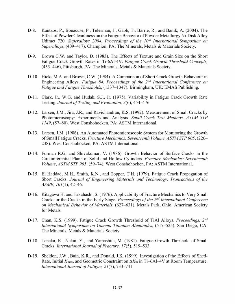
D-32

D-8. Kantzos, P., Bonacuse, P., Telesman, J., Gabb, T., Barrie, R., and Banik, A. (2004). The Effect of Powder Cleanliness on the Fatigue Behavior of Powder Metallurgy Ni-Disk Alloy Udimet 720. Superalloys 2004, Proceedings of the 10th International Symposium on Superalloys, (409–417). Champion, PA: The Minerals, Metals & Materials Society.

D-9. Brown C.W. and Taylor, D. (1983). The Effects of Texture and Grain Size on the Short Fatigue Crack Growth Rates in Ti-6Al-4V. Fatigue Crack Growth Threshold Concepts, (433–446), Pittsburgh, PA: The Minerals, Metals & Materials Society.

D-10. Hicks M.A. and Brown, C.W. (1984). A Comparison of Short Crack Growth Behaviour in Engineering Alloys. Fatigue 84, Proceedings of the 2nd International Conference on Fatigue and Fatigue Thresholds, (1337–1347). Birmingham, UK: EMAS Publishing.

D-11. Clark, Jr., W.G. and Hudak, S.J., Jr. (1975). Variability in Fatigue Crack Growth Rate Testing. Journal of Testing and Evaluation, 3(6), 454–476.

D-12. Larsen, J.M., Jira, J.R., and Ravichandran, K.S. (1992). Measurement of Small Cracks by Photomicroscopy: Experiments and Analysis. Small-Crack Test Methods, ASTM STP 1149, (57–80). West Conshohocken, PA: ASTM International.

D-13. Larsen, J.M. (1986). An Automated Photomicroscopic System for Monitoring the Growth of Small Fatigue Cracks. Fracture Mechanics: Seventeenth Volume, ASTM STP 905, (226–238). West Conshohocken, PA: ASTM International.

D-14. Forman R.G. and Shivakumar, V. (1986). Growth Behavior of Surface Cracks in the Circumferential Plane of Solid and Hollow Cylinders. Fracture Mechanics: Seventeenth Volume, ASTM STP 905. (59–74). West Conshohocken, PA: ASTM International.

D-15. El Haddad, M.H., Smith, K.N., and Topper, T.H. (1979). Fatigue Crack Propagation of Short Cracks. Journal of Engineering Materials and Technology, Transactions of the ASME, 101(1), 42–46.

D-16. Kitagawa H. and Takahashi, S. (1976). Applicability of Fracture Mechanics to Very Small Cracks or the Cracks in the Early Stage. Proceedings of the 2nd International Conference on Mechanical Behavior of Materials, (627–631). Metals Park, Ohio: American Society for Metals

D-17. Chan, K.S. (1999). Fatigue Crack Growth Threshold of TiAl Alloys. Proceedings, 2nd International Symposium on Gamma Titanium Aluminides, (517–525). San Diego, CA: The Minerals, Metals & Materials Society.

D-18. Tanaka, K., Nakai, Y., and Yamashita, M. (1981). Fatigue Growth Threshold of Small Cracks. International Journal of Fracture, 17(5), 519–533.

D-19. Sheldon, J.W., Bain, K.R., and Donald, J.K. (1999). Investigation of the Effects of Shed-Rate, Initial Kmax, and Geometric Constraint on ΔKth in Ti–6Al–4V at Room Temperature. International Journal of Fatigue, 21(7), 733–741.

D-33

D-20. Boyce B.L. and Ritchie, R.O. (2001). Effect of Load Ratio and Maximum Stress Intensity on the Fatigue Threshold in Ti-6Al-4V. Engineering Fracture Mechanics, 68(2), 129–147.

D-21. Slavik, D.C., Dunyak, T., Griffiths, J., and Kurath, P. (2000). Crack Initiation Modeling in Ti-6Al–4V for Smooth and Notched geometries. Proceedings, 5th National Turbine Engine High Cycle Fatigue Conference, Chandler, AZ.

D-22. Newman, J.C., Jr. (1984). A Crack-Opening Stress Equation for Fatigue Crack Growth. International Journal of Fracture, 24(4), R131–R135.

D-23. Van Stone, R.H. (1988). Residual Life Prediction Methods for Gas Turbine Components. Materials Science and Engineering, 103(1) 49–61.

D-24. Van Stone, R.H., Gilbert, M.S., Gooden, O.C., and Laflen, J.H. (1988). Constraint-Loss Model for the Growth of Surface Fatigue Cracks,” Fracture Mechanics: 19th Symposium, ASTM STP 969, (637–656). West Conshohocken, PA: ASTM International.

D-25. Newman, J.C., Jr. (1982). A Nonlinear Fracture Mechanics Approach to the Growth of Small Cracks. Proceedings of the 55th Meeting of the AGARD Structures and Materials Panel (AGARD-CP-328), Toronto, Canada.

D-26. Newman, J.C., Jr. and Yamada, Y. (2010). Compression Precracking Methods to Generate Near-Threshold Fatigue-Crack-Growth-Rate Data. International Journal of Fatigue, 32(6), 879–885.

D-27. Newman, J.C., Jr., Ruschau, J.J., and Hill, M.R. (2011). Improved Test Method for Very Low Fatigue-Crack-Growth-Rate Data. Fatigue and Fracture of Engineering Materials & Structures, 34(4), 270–279.

D-28. ASTM Standard E647-15e1, “Standard Test Method for Measurement of Fatigue Crack Growth Rates,” ASTM International, West Conshohocken, PA, 2015, DOI: 10.1520/E0647-15E01, www.astm.org

E-1

APPENDIX E—NICKEL ANOMALY FATIGUE TESTING

The objective of this activity was to characterize the impact of naturally occurring material anomalies on the fatigue performance of rotor-grade conventional nickel material—specifically, double melted IN-718. This involved the identification and procurement of material that appeared to contain significant material anomalies, forging and heat treatment of this material to rotor specification, additional NDE inspections, and the machining and testing of fatigue specimens for characterization. During the fatigue testing, the specimens received acoustic monitoring and an HCF “buzz” to assist in understanding the contribution of crack nucleation relative to crack growth life.

E.1 INITIAL INSPECTION AND SPECIMEN FABRICATION

Initial procurement and inspection of billets containing potential anomalies and specimen fabrication from these billets were performed in a previous grant (Turbine Rotor Material Design, Phase II) [E-1]. For completeness and convenience, the description of the inspection and specimen fabrication performed in the earlier grant is repeated here in this appendix.

E.1.1 ULTRASONIC INSPECTION OF IN-718 MULTS

Eight double-melt IN-718 billet sections (mults) of approximately 8″ diameter and identified by a supplier as having internal sonic indications were delivered to Pratt & Whitney (P&W) for further ultrasonic (UT) scanning. C-scans were made for each mult using a 5 MHz transducer with a focal length of 5″ and a diameter of 0.68″. The calibration setup was performed using flat entry samples with #1 flat-bottom hole (FBH). Calculations were made using the flaw response model developed at Iowa State University to account for the difference in the response between a flat entry surface and the curved entry surface of the mults. Also, the setup was made so that the #2 FBH response corresponded with 80% full screen height (FSH). Distance amplitude correction (DAC) was applied so that sensitivity was equivalent through the depth of the inspection. Each indication was identified and compared to the #2 FBH signal response and the spatial extent of the indications was recorded where possible.

Figure E-1 shows the c-scan for mult 804085-1A. The indication appeared to extend over a long circumferential distance because it was near the center at a depth of 3.7″. The 60o length of the indication corresponds to 0.31″, and the position of highest amplitude corresponds to approximately 60% of a #2 FBH. It could not be determined from the UT data whether the apparent anomaly contained voids, foreign material, or an aberrant grain structure. It appeared, however, that there was a noisy grain structure because there was weak UT response spread throughout the c-scan. Because the indication was near the centerline, and other regions in the c-scan correspond to the appearance of large grain structure, it is likely that the apparent anomaly was actually due to large grains. The color bar shown in figure E-1 applies to all the c-scan images of the mults and the pancakes.

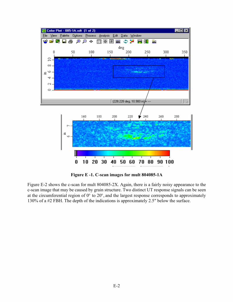
E-2

Figure E -1. C-scan images for mult 804085-1A

Figure E-2 shows the c-scan for mult 804085-2X. Again, there is a fairly noisy appearance to the c-scan image that may be caused by grain structure. Two distinct UT response signals can be seen at the circumferential region of 0 to 20, and the largest response corresponds to approximately 130% of a #2 FBH. The depth of the indications is approximately 2.5″ below the surface.

E-3

Figure E-2. C-scan images for mult 804085-2X: (a) full c-scan and (b) concentrated re-scan in region of largest reflectors

The c-scan image for mult 804085-3A is shown in figure E-3, and the “noisy” structure is apparent. What appears to be an inclusion at 90% of #2 FBH sensitivity may be a higher concentration of large grains. The grain noise is most apparent nearer the center of the billet because the noise is amplified by the application of DAC, and the values plotted in the c-scan are primarily from near the billet center.

(a)

(b)

(a)

(b)

E-4

Figure E-3. C-scan image for 804085-3A

Figure E-4 shows the c-scan image for mult 804085-3X, and it is apparent that six distinct features are present. All of the features are at depths between 2.25″ and 2.5″, and the largest reflector has an amplitude that is 190% of a #2 FBH. The calculated beam width at a depth of 2.5″ is 0.3″ in the circumferential direction and 0.23″ in the axial direction, and those are the approximate dimensions of the features identified in the c-scan. Therefore, the features have spatial extent that is less than the dimensions of the beam and can be considered point reflectors.

E-5

Figure E-4. C-scan image of mult 804085-3X

Figure E-5 shows the c-scan image for mult 804618-5A1 with a distinct feature near the center of the billet. The feature has an amplitude of 200% of a #2 FBH and is at a depth of approximately 3.7″.

E-6

Figure E-5. C-scan image for 804618-5a1: (a) full c-scan and (b) concentrated re-scan without signal saturation

Mult 804618-5A2 is a separate billet section from the mult labeled 5A1. The c-scan image for 5A2 is shown in figure E-6. The indication is at a depth of 3.3″ and is likely smaller than the dimensions of the beam. The reflected amplitude for this indication is approximately 40% of a #2 FBH.

(a)

(b)

(a)

(b)

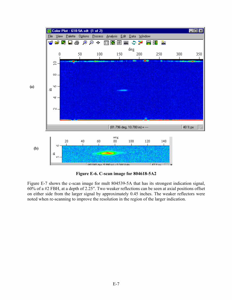
E-7

Figure E-6. C-scan image for 804618-5A2

Figure E-7 shows the c-scan image for mult 804539-5A that has its strongest indication signal, 60% of a #2 FBH, at a depth of 2.25″. Two weaker reflections can be seen at axial positions offset on either side from the larger signal by approximately 0.45 inches. The weaker reflectors were noted when re-scanning to improve the resolution in the region of the larger indication.

(a)

(b)

(a)

(b)

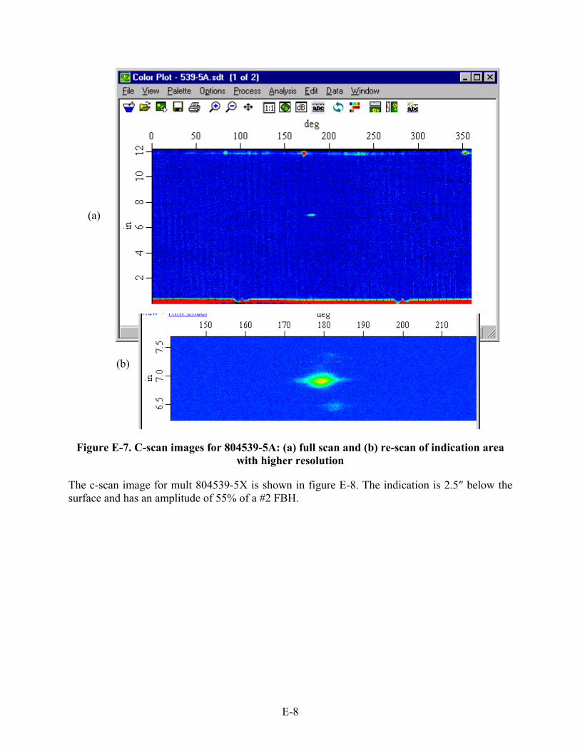
E-8

Figure E-7. C-scan images for 804539-5A: (a) full scan and (b) re-scan of indication area with higher resolution

The c-scan image for mult 804539-5X is shown in figure E-8. The indication is 2.5″ below the surface and has an amplitude of 55% of a #2 FBH.

(a)

(b)

E-9

Figure E-8. C-scan image of 804539-5X

E.1.2 ULTRASONIC INSPECTION OF IN-718 FORGED PANCAKES

After the 8″ diameter mults were forged to the pancake shape of 16″ diameter and 2.9″ thick, UT inspections were performed to determine the positions of the indications. The pancakes as received at P&W had a surface finish with significant machining grooves that caused a high-amplitude ringdown signal in some of the pancakes. An example of the ringdown is shown in figure E-9. This ringdown was thought to be masking the indication signals in some of the pancakes. Indications were seen in only three of the eight pancakes. Efforts within the lab to reduce the effects of the machining grooves with a hand-held grinding wheel were not sufficient, and the pancakes were sent to a supplier that was able to apply a ground surface to the pancakes.

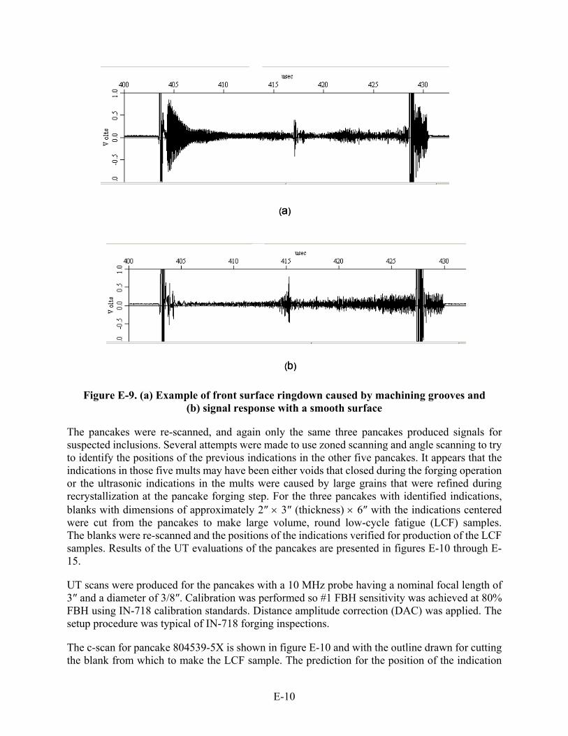
E-10

Figure E-9. (a) Example of front surface ringdown caused by machining grooves and (b) signal response with a smooth surface

The pancakes were re-scanned, and again only the same three pancakes produced signals for suspected inclusions. Several attempts were made to use zoned scanning and angle scanning to try to identify the positions of the previous indications in the other five pancakes. It appears that the indications in those five mults may have been either voids that closed during the forging operation or the ultrasonic indications in the mults were caused by large grains that were refined during recrystallization at the pancake forging step. For the three pancakes with identified indications, blanks with dimensions of approximately 2″ 3″ (thickness) 6″ with the indications centered were cut from the pancakes to make large volume, round low-cycle fatigue (LCF) samples. The blanks were re-scanned and the positions of the indications verified for production of the LCF samples. Results of the UT evaluations of the pancakes are presented in figures E-10 through E-15.

UT scans were produced for the pancakes with a 10 MHz probe having a nominal focal length of 3″ and a diameter of 3/8″. Calibration was performed so #1 FBH sensitivity was achieved at 80% FBH using IN-718 calibration standards. Distance amplitude correction (DAC) was applied. The setup procedure was typical of IN-718 forging inspections.

The c-scan for pancake 804539-5X is shown in figure E-10 and with the outline drawn for cutting the blank from which to make the LCF sample. The prediction for the position of the indication

(a)

(b)

(a)

(b)

E-11

using DEFORM was 5.7″ radially and 1.5″ deep. The position of the indication was very close to the predicted position with a radial position of 5.8″, a depth from one side of the pancake of 1.5″, and a depth from the other side of 1.3″. Figure E-11 shows a higher resolution scan at a shorter water path with a box drawn around the indication of dimension 0.4″ 0.4″. The largest UT response from the features within the box corresponds to ~100% of #1 FBH, but the extent of the indication is obviously larger than the 0.016″ diameter of a #1 FBH.

Figure E-10. C-scan of pancake 804539-5X with setup of #1 FBH sensitivity

2.0”6.5”

804539

5x

2.0”6.5”

804539

5x

E-12

Figure E-11. C-scan of indication in pancake 804539-5X with focus closer to the indication to provide more resolution

The c-scan for pancake 804539-5A is shown in figure E-12 with the outline drawn on the c-scan image for cutting the blank from which to make the LCF sample. The position of the indication is very close to the position predicted by DEFORM. DEFORM predicted a radial position of 4.8″ and a depth of 1.5″, and the indication was actually at 5.0″ radially and 1.3 to 1.5″ deep. Figure E-13 shows a higher resolution scan at a shorter water path with a box drawn around the indication of dimension 0.6″ 0.4″. The largest UT response from the features within the box corresponds to ~50% of #1 FBH, but the extent of the indication is obviously larger than the 0.016″ diameter of a #1 FBH.

E-13

Figure E-12. C-scan of pancake 804539-5A with setup of #1 FBH sensitivity

6.5”

2.0”

804539-5a

6.5”

2.0”

804539-5a

E-14

Figure E-13. C-scan of indication in pancake 804539-5A with focus closer to the indication to provide more resolution

The c-scan for pancake 804618-5A is shown in figure E-14 with the outline drawn on the c-scan image for cutting the blank from which to make the LCF sample. The position of the indication is very close to the position predicted by DEFORM. DEFORM predicted a radial position of 1.2″ and a depth of 1.5″; the actual radial position was 1.4″ and the depth was 1.5″. Figure E-15 shows a higher resolution scan at a shorter water path with a box drawn around the indication of dimension 0.6″ x 0.8″. The largest UT response from the features within the box corresponds to ~125% of #1 FBH, but the extent of the indication is seen to nearly fill the 0.6 0.8″ box and is significantly larger than the 0.016″ diameter of a #1 FBH.

E-15

Figure E-14. C-scan of pancake 804618-5A with setup of #1 FBH sensitivity

6.5”

2.0”

804618-5a

6.5”

2.0”

804618-5a

E-16

Figure E-15. C-Scan of indication in pancake 804618-5A with focus closer to the indication to provide more resolution

After removing the blanks from the three pancakes, scans were made to assure that the features were centered in the blanks. Measurements were made to define the positions of the indications with respect to the edges of the blanks, and the edges of the blanks were determined by scanning the top of the blank with the UT beam focused on the surface. The region of the indication was then re-scanned with the same coordinates system. Based on the resulting measurements, detailed fatigue specimen machining drawings were developed in an attempt to center the inclusions in the gauge section.

E-17

E.2 FATIGUE TESTING

Three cylindrical specimens with 0.5″-diameter gauge sections were machined from the five forgings containing embedded indications. A representative specimen is shown in figure E-16.

Figure E-16. Cylindrical fatigue specimen containing embedded defect

After machining, the specimens were inspected by fluorescent penetrant inspection. One of the specimens contained surface indications believed to be one of the embedded indications, which had become surface connected (see figure E-17). The specimens were shot peened before testing to retard crack formation on the surface and encourage crack formation at the embedded indications.

Figure E-17. IN-718 specimen MWF6116 gauge section prior to shot peening

The specimen test matrix is given in table E-1. The first of the three specimens (MWF6116) fractured prematurely on the initial upload cycle because of a failure of the test rig controller. The second and third specimens (MWF6114 and MWF6115) completed testing successfully, running for 114,976 cycles and 43,684 cycles, respectively.

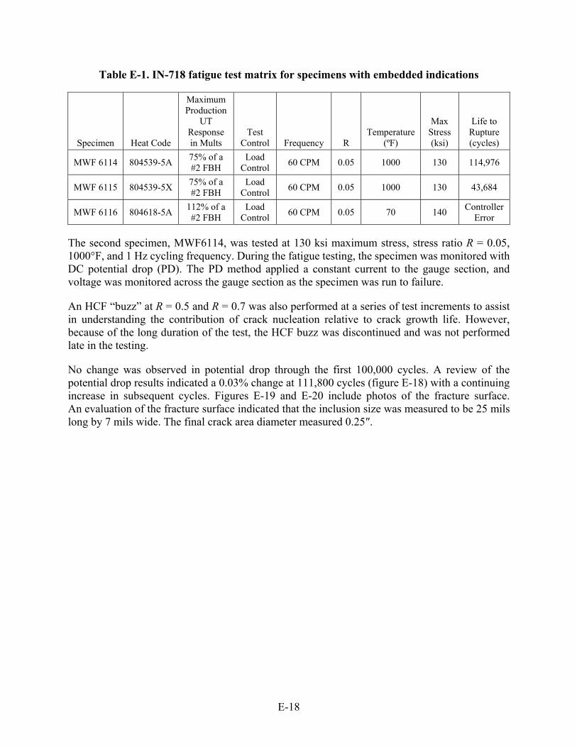
E-18

Table E-1. IN-718 fatigue test matrix for specimens with embedded indications

Specimen Heat Code

Maximum Production

UT Response in Mults

Test Control Frequency R

Temperature (ºF)

Max Stress (ksi)

Life to Rupture (cycles)

MWF 6114 804539-5A 75% of a #2 FBH

Load Control

60 CPM 0.05 1000 130 114,976

MWF 6115 804539-5X 75% of a #2 FBH

Load Control

60 CPM 0.05 1000 130 43,684

MWF 6116 804618-5A 112% of a #2 FBH

Load Control

60 CPM 0.05 70 140 Controller

Error

The second specimen, MWF6114, was tested at 130 ksi maximum stress, stress ratio R = 0.05, 1000°F, and 1 Hz cycling frequency. During the fatigue testing, the specimen was monitored with DC potential drop (PD). The PD method applied a constant current to the gauge section, and voltage was monitored across the gauge section as the specimen was run to failure.

An HCF “buzz” at R = 0.5 and R = 0.7 was also performed at a series of test increments to assist in understanding the contribution of crack nucleation relative to crack growth life. However, because of the long duration of the test, the HCF buzz was discontinued and was not performed late in the testing.

No change was observed in potential drop through the first 100,000 cycles. A review of the potential drop results indicated a 0.03% change at 111,800 cycles (figure E-18) with a continuing increase in subsequent cycles. Figures E-19 and E-20 include photos of the fracture surface. An evaluation of the fracture surface indicated that the inclusion size was measured to be 25 mils long by 7 mils wide. The final crack area diameter measured 0.25″.

E-19

Figure E-18. Potential drop results for Ni anomaly specimen MWF 6114

Figure E-19. Inclusion observed on fracture surface of specimen MWF 6114

E-20

Figure E-20. Fracture surface for specimen MWF 6114

The third specimen, MWF 6115, was tested at the same conditions of 130 ksi maximum stress, stress ratio R = 0.05, 1000°F, and 1 Hz cycling frequency as MWF 6114. The cylindrical, axially loaded sample, with a gauge section diameter of ~0.500 inch, contained a defect in its center. Post-test fractography found that the defect had a 0.0293″ × 0.0522″ cross-section.

Direct-current potential drop (DCPD) measurements were taken in an attempt to monitor fatigue crack growth from the embedded defect. DCPD data were initially stored every 200 cycles and then more often after detection of a crack. A fracture-surface marker band was created after a 0.2% change in DCPD by switching to R = 0.7 for approximately 2000 cycles. A second marker band was created after a 1.4% change in DCPD by switching to R = 0.7 for approximately 1,000 cycles. The sample failed after 43,684 cycles. Figure E-21 shows the fracture surface.

Results of the testing are shown in figure E-22. Here, the crack-length values are based on DCPD measurements, calibrated to post-test fractography. Just as with the earlier test, which failed at 114,976 cycles from a smaller flaw size, this sample exhibited a significant incubation period (flat portion of the crack growth curve) before active crack growth from the defect began.

E-21

Figure E-21. Fracture surface for specimen MWF 6115

Figure E-22. Crack-growth behavior for specimen MWF 6115

0 10000 20000 30000 40000 50000Cycle Count

0.000

0.020

0.040

0.060

0.080

0.100

0.120

0.140

0.160

0.180

0.200

Cra

ck L

ength

(in

)

0.00

0.50

1.00

1.50

2.00

2.50

3.00

3.50

4.00

4.50

5.00

Cra

ck L

eng

th (

mm

)INCO 718R = 0.05

1000 deg F

Symbol Test ID 17213

Crack Size vs. Cycle Count

E-22

Two photographs from the fractographic study are shown in figure E-23. The top photo shows the primary buried defect and the circular marker bands produced on the fracture surface during the test. The defect was found to be aluminum rich. The photo also indicates that a small cluster of secondary buried flaws was found near the primary defect. These secondary flaws did not appear to form any secondary cracks. The primary defect is shown more closely in the bottom photo.

Figure E-23. Photographs of fracture surface from specimen MWF 6115

E-23

E-3. RE-INSPECTION OF NICKEL ANOMALY BILLETS

Other than the three indications used to fabricate fatigue test specimens, none of the other indications originally detected in the initial billet inspection could be found. Efforts to find the remaining eight defects post forging were unsuccessful, despite inspection at DEFORM-predicted depths and angled scans. Subsequent processing of the remaining forgings (see table E-2) included etch inspection and machining of the as-forged surface from the end of the forging for additional sonic inspections.

Table E-2. Billet inspection results

Indication Heat

Maximum Production UT

Response in Mults

Maximum Laboratory UT

Response in Mults

Maximum Laboratory UT

Response in Pancakes

1A 804085 110% of #2 FBH 60% of #2 FBH Not Found

XXX 804085 110% of #2 FBH 130% of #2 FBH Not Found

3A 804085 110% of #2 FBH 90% of #2 FBH Not Found

3X 804085 160% of #2 FBH 190% of #2 FBH Not Found

5A 804618 112% of #2 FBH 200% of #2 FBH 125% of #1 FBH*

804618 75% of #2 FBH 40% of #2 FBH Not Found

5A 804539 75% of #2 FBH 60% of #2 FBH 50% of #1 FBH*

5X 804539 75% of #2 FBH 55% of #2 FBH 100% of #1 FBH* Indications highlighted in blue were machined into test specimens

Additional machining and inspection of one of the forgings was performed in an attempt to find the “missing” defects. This work was supported with funds provided outside of the FAA grant. This pancake forging (see figure E-24) was ultrasonically inspected using both a single-element normal incidence from top, bottom, and side, and a phase array probe. The 10 MHz probe/array found no indications and inspected down to a sensitivity of 8 mils.

Figure E-24. Machined pancake forging (3X, heat 80485)

E-24

P&W shipped two of the remaining forgings, including the forging pictured in figure E-24, to GE Aviation (GEA) for further inspection at GE. GE used a multizone inspection technique based on a customized transducer and sound beam to provide maximum sensitivity. The purpose of this inspection effort was to find anomalies in the forgings (if they existed) with the best inspection technique available at GEA. As such, the inspection technique used would not be considered a production inspection method, but was instead a high-fidelity laboratory inspection technique. The two forgings were inspected with a multizone approach, using ~12 MHz transducers with a depth of field of 0.25″ in metals. All material was inspected within the focal zone of this transducer and, therefore, each 3″ thick forging required 7 scans from each side for full coverage, for a total of 14 scans. Most scans showed nothing of interest. Some indications were found in a small number of scans. These indications fall into three general categories: 1) pockets of material on the part surface, filled in with smeared metal, containing relatively large (up to ~250 mils) defects near the surface; 2) very small “pinpoint” indications, characteristic of very small subsurface defects (<5 mils); and 3) discrete changes in grain structure. No subsurface defects larger than 5 mils were found.

P&W worked with GE to resolve questions regarding how comparable previous inspections conducted by P&W of these two IN-718 forgings were to those recently conducted by GE. The two forging inspections at P&W had been previously reported to have not shown any indications greater than 8 mils in the machined forging and nothing greater than 16 mils in the unmachined forging. Although the more-detailed GE inspections did locate defects in both forgings, neither forging appears to have indications of a size that would merit fabricating new specimens. GE inspections did not refute the inspection findings of the previous P&W inspections.

E.4. INVESTIGATION OF FRECKLES

An additional set of three IN-718 mults containing surface-connected freckles was also obtained during the TRMD Phase II program. The three mults were forged, heat treated, sonic inspected, and macro etched prior to marking the Laves-rich freckles areas to be turned into specimens. The Laves phase is a topologically close packed brittle intermetallic phase that forms as a result of solidification segregation. Fatigue cracks resulting from freckles are expected to originate from cleavage through Laves particles contained in the freckles. A preliminary test plan for samples containing freckles was proposed and agreed on by the PDRI team. This proposed test plan is shown in table E-3.

Table E-3. P&W proposed matrix for IN-718 freckle testing

Temperatures Tensile LCF Crack

Growth

Baseline Defect/ In-situ Stress Level Baseline Defect Defect

(F) (Number) (Number) (Number) (Number)

800 2 4 Hi 4 6 1

Low 4 6

1100 2 4 Hi 4 6 1

E-25

The testing was delayed pending the outcome of proposed RISC activity under which each of the OEMs would contribute existing proprietary freckle test data. These data were to be pooled together and used by the industry in lieu of the originally planned testing under the PDRI program. RISC released a spreadsheet for data collection in July 2009 (see figure E-25) to be filled out by the RISC members. However, this data-collection task was not completed. By the time it became apparent that the data-collection task would not be completed, insufficient time or budget remained in the PDRI program to perform the originally planned testing.

Figure E-25. Spreadsheet circulated to RISC members to collect information on fatigue-testing experience with naturally occurring nickel anomalies

E-26

E.5. REFERENCE

E-1. FAA Report. (2008). Turbine Rotor Material Design—Phase II. (DOT/FAA/AR-07/13)

F-1

APPENDIX FBENCHMARK FATIGUE CRACK-GROWTH TESTING

Engineering stress intensity factor (SIF) solutions are commonly verified analytically by comparison to more sophisticated numerical solutions. However, even the exact numerical solutions can exhibit some variability, depending on the quality of the method and the skill of the modeler. SIF solutions developed by different organizations for the same nominal geometry can exhibit noticeable differences. Furthermore, the ability of the mathematical SIF solutions alone to address geometrical effects, such as the interaction of the crack front with adjoining or approaching free surfaces, is remarkably unresolved in the literature. Experimental validation is needed to ensure that SIF solutions are formulated and implemented to give accurate predictions of fatigue crack growth (FCG) rate.

In this activity, a reliable database of FCG data from several different specimen geometries was generated for a carefully pedigreed rotor material to facilitate the evaluation of SIF solutions and related crack-growth algorithms in the Design Assessment of Reliability With Inspection (DARWIN®) Flight_Life fracture mechanics module. All testing was performed at Honeywell on a fine-grained delta-processed Inconel 718 alloy (DP718) at 600F. Testing was performed on four different specimen geometries: surface-crack tension (SC(T)) specimens with two different thicknesses, a corner-crack tension (CC(T)) specimen, and a center-hole specimen with a corner crack at the hole. Analysis of the resulting data was performed at SwRI®. Additional benchmark experiments were originally planned to be performed at SwRI with Ti-6Al-4V specimens testing at room temperature, but these tests could not be performed because of unexpected reductions in the grant budget. This work is planned for a subsequent grant. F.1 MATERIAL AND SPECIMEN PREPARATION

The material employed in this testing was delta-processed Inconel 718 alloy (DP718) with an ASTM grain size of 10 to 12, a yield strength of 169 ksi, and an ultimate tensile strength of 205 ksi. DP718 billet is made from triple-melt ingot through vacuum-induction melting (VIM), followed by electroslag remelting and finished by vacuum arc remelting (VAR). A DP718 forging derives its strength benefits from a consistently fine microstructure, which is a result of a delta-processing treatment of the raw material when it is being manufactured into billet. The processing occurs during initial ingot breakdown when a special delta-phase precipitation heat treatment is added to the normal billet manufacture. This heat treatment essentially consists of a long soak for 24 hours at approximately 1650ºF. The delta phase consists of Ni3Nb precipitates, which act to inhibit grain growth from any potential recrystallization operations during final billet working. After the delta-phase heat treatment, final billet working is performed at temperatures less than the delta-solvus to ensure fine microstructure. Forging temperatures are generally well below typical delta-solvus temperatures of 1850ºF to 1875ºF, which also ensures that the fine microstructure is maintained.

After forging, the final heat treatment of DP718 consists of a solution treatment below (delta) δ-solvus, followed by a two-step aging process. The solution temperature is typically held near the δ-solvus to avoid grain growth. Because the δ-solvus is in the range of 1850ºF to 1875ºF, the solution temperatures often range from 1800ºF to 1850ºF to maintain a fine microstructure while achieving the best γ precipitation possible. The first and second age cycles result in precipitates,

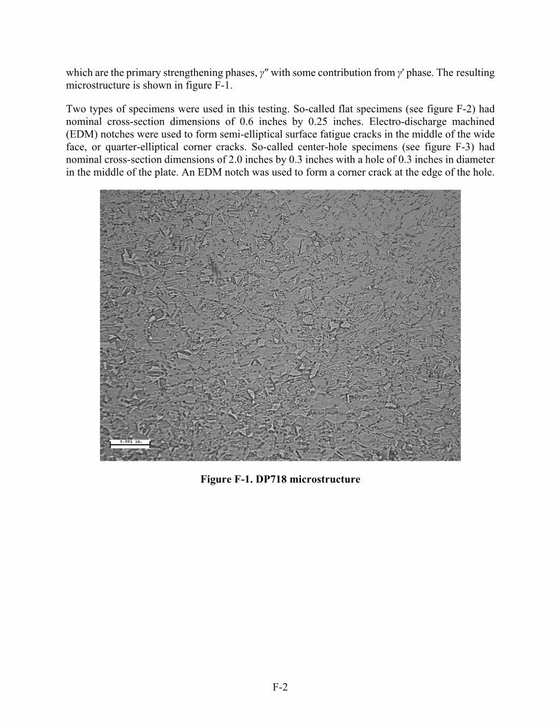
F-2

which are the primary strengthening phases, γ″ with some contribution from γ′ phase. The resulting microstructure is shown in figure F-1.

Two types of specimens were used in this testing. So-called flat specimens (see figure F-2) had nominal cross-section dimensions of 0.6 inches by 0.25 inches. Electro-discharge machined (EDM) notches were used to form semi-elliptical surface fatigue cracks in the middle of the wide face, or quarter-elliptical corner cracks. So-called center-hole specimens (see figure F-3) had nominal cross-section dimensions of 2.0 inches by 0.3 inches with a hole of 0.3 inches in diameter in the middle of the plate. An EDM notch was used to form a corner crack at the edge of the hole.

Figure F-1. DP718 microstructure

F-3

Figure F-2. Flat FCG specimen drawing

Figure F-3. Center-hole FCG specimen drawing

F-4

The near-surface residual stresses remaining after low stress grinding (LSG) machining by MAR-TEST (see figure F-4 for the residual stress distributions) were deemed unacceptably high for the purpose of this study. Therefore, specimens were longitudinally polished (see Table F-1 for the surface residual stress results) and then electro-polished by Lambda Technologies to remove at least 0.0005″ and to reduce the surface residual stress to an acceptable level. The specimens were then returned to MAR-TEST for EDM notching. The material along the anticipated crack trajectory on the specimen face was mechanically polished at Honeywell to facilitate optical observation and measurement.

Figure F-4. Residual stress distribution in the specimen near-surface layer after LSG machining

Table F-1. Surface residual stress in two arbitrarily chosen specimens after longitudinal polishing

LONGITUDINAL RESIDUAL STRESSES IN-718 CRACK GROWTH SPECIMENS

Mid-Length Location After Mar-Test Polishing

Specimen ID Depth RESIDUAL STRESS PEAK WIDTH (deg.)

(in.) (mm) (ksi) (MPa)

B8 0.0005 0.013 +6.2 ± 1 +43 ± 7 1.49

D3 0.0005 0.013 +0.2 ± 2 +1 ± 14 1.88

0 1 2 3 4 5 6 7 8 9 10-80

-70

-60

-50

-40

-30

-20

-10

0

10

20

30

C7

Res

idua

l Str

ess

(ksi

)

Depth (x 10-3 in.)

0 20 40 60 80 100 120 140 160 180 200 220 240

-500

-400

-300

-200

-100

0

100

200

Residual S

tress (MP

a)

Depth (x 10-3 mm)

LONGITUDINAL RESIDUAL STRESS DISTRIBUTION

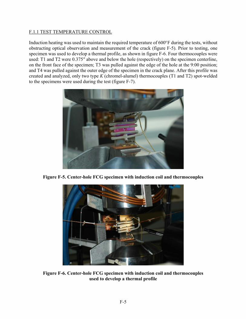
F-5

F.1.1 TEST TEMPERATURE CONTROL

Induction heating was used to maintain the required temperature of 600F during the tests, without obstructing optical observation and measurement of the crack (figure F-5). Prior to testing, one specimen was used to develop a thermal profile, as shown in figure F-6. Four thermocouples were used: T1 and T2 were 0.375″ above and below the hole (respectively) on the specimen centerline, on the front face of the specimen; T3 was pulled against the edge of the hole at the 9:00 position; and T4 was pulled against the outer edge of the specimen in the crack plane. After this profile was created and analyzed, only two type K (chromel-alumel) thermocouples (T1 and T2) spot-welded to the specimens were used during the test (figure F-7).

Figure F-5. Center-hole FCG specimen with induction coil and thermocouples

Figure F-6. Center-hole FCG specimen with induction coil and thermocouples used to develop a thermal profile

F-6

Figure F-7. Center-hole specimen instrumented with two type K (chromel-alumel) thermocouples

F.1.2 CRACK SIZE MEASUREMENT

A long-distance microscope (Questar QM100) was used to observe and periodically measure the crack on the specimen surface during the tests, as shown in figure F-8. In addition, several heat tints were conducted during each test to mark the entire crack front corresponding to the current surface measurements. An example of a heat-tinted fracture surface is shown in figure F-9. Additional measurements were made on the heat-tinted surfaces following completion of each test. Also, several attempts were made to mark the current crack front by altering load parameters. It should be noted that the optical crack-length measurement at the beginning of the test performed on center-hole specimens and flat specimens with corner notches was extremely difficult and time consuming because of rounding of the specimen edges by electro-polishing.

F-7

Figure F-8. Surface crack-size measurements with Questar QM100

Figure F-9. Heat-tinted fracture surface for specimen A3

F.1.3 PRE-CRACKING

Prior to testing, all specimens were pre-cracked in compression at room temperature. Pre-cracking was conducted with a maximum stress of 0 ksi and a minimum stress of -130 ksi for all specimens. To determine the necessary number of cycles, one specimen of each type was periodically

F-8

observed until no further crack growth could be optically detected on the specimen surface. The same number of load cycles was applied to pre-crack all remaining specimens of the same type. Following this procedure, all specimens were subjected to heat tinting to mark the pre-crack.

F.2 TESTING

All specimens were tested in laboratory air at 600F using servo-hydraulic MTS frames with Fracture Technology Associates (FTA) software. The applied stress ratio was R = 0.05. A triangular wave-shape of constant-load amplitude was applied with a frequency of 1 Hz. On several occasions, high-frequency loading (15 Hz sine waveform) was applied temporarily in an attempt to mark the current crack front.

Table F-2 summarizes the specimens and test conditions for the benchmark testing. The stress values in this table are the maximum nominal remote stresses in the SC(T) and CC(T) specimens, and the maximum nominal net-section stresses in the center-hole specimen.

Table F-2. Specimens and test conditions for benchmark FCG testing

ID Specimen Type Maximum

Stress A1 SC(T) 63 ksi A3 SC(T) 63 ksi A4 SC(T) 63 ksi B6 SC(T) 110 ksi C5 CC(T) 63 ksi C7 CC(T) 64 ksi B5 SC(T) 110 ksi C6 CC(T) 100 ksi C8 CC(T) 100 ksi B8 Thin SC(T) 64 ksi C1 Center Hole 30 ksi C2 Center Hole 30 ksi B2 Center Hole 39.5 ksi

Nine flat specimens with EDM notches were tested. Specimens A1, A3, A4, B5, B6, C5, C6, C7, and C8 had nominal cross-sectional dimensions of 0.6″ by 0.25″, whereas a “thin” specimen B8 had nominal cross-sectional dimensions of 0.6″ by 0.1″. Five of the tested specimens had an SC(T) geometry and four (C5, C6, C7, and C8) had a CC(T) geometry. Crack-length measurements for specimen B6 were not accurate, so the data were not used.

A total of three center-hole specimens were tested. Specimens C1 and C2 were tested at identical conditions, whereas specimen B2 was tested at a larger stress amplitude. Useful data were obtained only from specimens C1 and B2.

F-9

F.3 DATA ANALYSIS

As noted previously, the basic paradigm of the benchmarking process is that FCG data from one simple specimen type are used to establish reliable baseline properties, and then these properties are independently used to predict the crack growth behavior for other specimen types.

For the Honeywell tests on DP718, the results using the SC(T) geometry were used to establish the baseline properties. The DARWIN SC17 solution was used to calculate the SIF for each measured crack length. The value of ΔK at the surface tip (the c-tip) was multiplied by the DARWIN constraint correction factor (β = 0.9 at R = 0.05). The crack-growth rate da/dN was calculated from the raw a versus N data using standard ASTM seven-point incremental polynomial methods.

As noted previously, crack-length measurements were obtained by two different methods. Optical measurements were taken on the specimen surface throughout the test. Post-test fractography was used to determine the surface length and depth of the crack at a limited number of heat tints. The two-dimensional shape information could then be used to estimate the crack depth for those optical measurements without a directly corresponding heat-tint measurement, by interpolation from the nearest heat-tint measurements. However, in several cases, the measured surface crack (SC) length obtained from direct optical and fractographic heat-tint methods did not agree for the same cycle count in the test. In these situations, some judgment was required to adjust the optical measurements and the corresponding crack depths to generate a consistent set of data.

Compression pre-cracking methods have been shown to influence FCG data during the regular cycling that occurs after the compression pre-cracking has been completed, until the crack has grown beyond the influence of the crack-tip plastic zone from the compression pre-cracking (generally approximately two or three times the final crack-tip plastic zone width). Therefore, some early data from the regular cycling were censored so that anomalous behavior would not be included in the generation of baseline properties or in the benchmarking comparisons.

The resulting da/dN versus ΔK data for the combined SC tests are shown in figure F-10. Also shown in this graph is the regression line for the Paris equation fit to the data. Note that only the surface length (“c” tip) values are shown, and only the surface length values were used in the regression to determine the Paris equation constants.

F-10

Figure F-10. Crack-growth rate data for SC(T) specimens and corresponding Paris equation regression line

Figure F-11 shows how this Paris equation fit was used in DARWIN to predict the crack-length-versus-cycles data from one of the baseline SC(T) tests. The close agreement between the predicted and actual crack-length curves confirms that the Paris equation was an acceptably accurate fit to the original data. Note that data from both the “a” tip and the “c” tip are included in this graph. Similar direct comparisons are more difficult to perform for the other SC(T) tests because they included non-negligible crack growth during marker band cycling at different stress ratios for which baseline growth rate data were not available.

Once the baseline crack growth properties (Paris equation constants) were established from the SC(T) specimens, these same properties were used to predict the crack-growth behavior in the flat CC(T) specimens. No data from the CC(T) specimens were employed to predict growth in the CC(T) specimens; the predictions were truly independent. The DARWIN CC11 solution was used to calculate the SIF. As for the SC(T) tests, some adjustments were required to reconcile the optical and heat-tint measurements, and some early data were censored to remove the anomalous influence of the compression pre-cracking.

K (ksiin)

1 10 100

dc/d

N (

in/c

ycle

)

1e-7

1e-6

1e-5

1e-4

Test data (SCT)Paris fit

F-11

Figure F-11. Experimental and predicted crack-growth history for SC(T) specimen A1

Figures F-12, F-13, and F-14 compare the predicted and measured crack-length-versus-cycles results for CC(T) specimens C-5, C-6, and C-8, respectively. Note that both the a tip and c tip data are included on these graphs. There are also two sets of predicted curves on each graph. In one prediction, the same constraint correction factor (β) is employed at both tips. In the other prediction, the constraint correction factor is NOT employed at either tip. The reason for making this comparison is described in the following two paragraphs.

For the SC(T) geometry used to generate the baseline data, numerous researchers over the years have demonstrated that the constraint correction factor is necessary to make accurate predictions. The uncorrected SIF solution for this geometry is approximately 10% higher at the surface tip (“c” tip) than at the maximum depth tip (“a” tip). This would predict that the stable aspect ratio a/c of a growing semi-elliptical SC under uniform tension fatigue loading should be less than 1. However, numerous experimental studies have shown that the stable shape of this crack is approximately 1 in most cases. This result is properly predicted if the constraint correction factor β = 0.9 is applied to the surface tip ΔK values.

For the CC(T) geometry, this comparison is not as easy to make, because the constraint correction factor should be applied (or not) at both tips, so the aspect ratio of the crack would not change. As a result, it has never been clearly established in the research literature whether the constraint correction factor should be applied to corner cracks in fatigue. Some protocols and computer codes (including both DARWIN and NASGRO) have included the factor for CC(T) analysis, and some have not included it. To determine whether it should be included, it is necessary to generate very-high-quality data—which is the design of this study.

Surface Crack Tension (A1)

N (cycles)

0.0 2.0e+4 4.0e+4 6.0e+4 8.0e+4 1.0e+5 1.2e+5 1.4e+5

a &

c (

in)

0.00

0.05

0.10

0.15

0.20

0.25

Test (a-tip)Test (c-tip)Prediction (a-tip)Prediction (c-tip)

F-12

Figure F-12. Comparison of experimental and independently predicted crack-growth behavior for CC(T) specimen C5

Figure F-13. Comparison of experimental and independently predicted crack-growth behavior for CC(T) specimen C6

Corner Crack Tension (C5)

N (cycles)

0 2e+4 4e+4 6e+4 8e+4 1e+5

a &

c (

in)

0.00

0.05

0.10

0.15

0.20

0.25

0.30

Test (c-tip)Test (a-tip)Prediction (no beta correction, c-tip)Prediction (no beta correction, a-tip)Prediction (beta correction, c-tip)Prediction (beta correction, a-tip)

Corner Crack Tension (C6)

N (cycles)

0 5000 10000 15000 20000 25000 30000

a &

c (

in)

0.00

0.05

0.10

0.15

0.20

0.25

0.30

Test (c-tip)Test (a-tip)Prediction (no beta correction, c-tip)Prediction (no beta correction, a-tip)Prediction (beta correction, c-tip)Prediction (beta correction, a-tip)

F-13

Figure F-14. Comparison of experimental and independently predicted crack-growth behavior for CC(T) specimen C8

With respect to figures F-12–F-14, it appears that the predictions that do employ the constraint correction factors are, on average, better than the predictions that do not employ the constraint correction factors. This determination must also consider the natural test-to-test scatter that has occurred in these three tests. The predictions, including β, are slightly conservative for specimen C5 (figure F-12), quite accurate for specimen C6 (figure F-13), and slightly nonconservative for specimen C-8 (figure F-14). In contrast, the predictions that do not include β are very conservative for C5, conservative for C6, and relatively accurate for C8. This result appears to confirm that the DARWIN approach of using the CC11 SIF solution with the constraint correction factor included gives accurate crack-growth predictions. However, caution should be observed regarding drawing definitive conclusions from one dataset.

The baseline properties derived from the SC(T) tests were also used to predict the corner-crack-at-hole tests. To perform this prediction using DARWIN, it was first necessary to build a three-dimensional ANSYS model of the test specimen from which the appropriate stress gradients could be extracted on the stress plane. The univariant CC08 SIF solution was used. The transition to a through-crack geometry was not included in the comparisons. Once again, as in the studies of the corner-crack-in-plate geometry, two calculations were performed. One calculation (the default DARWIN mode) included the constraint correction at both surface tips of the corner crack. A second calculation removed this constraint correction for comparison.

The experimental a versus N results for tests B2 and C1 are shown in figure F-15, along with predictions for B2. The test results for B2 fall between the two predictions, somewhat closer to the predictions that do not include the constraint correction. Unfortunately, the experimental results

Corner Crack Tension (C8)

N (cycles)

0 5000 10000 15000 20000 25000 30000

a &

c (

in)

0.00

0.05

0.10

0.15

0.20

0.25

0.30

Test (c-tip)Test (a-tip)Prediction (no beta correction, c-tip)Prediction (no beta correction, a-tip)Prediction (beta correction, c-tip)Prediction (beta correction, a-tip)

F-14

indicate some scatter that may call into question the diagnostic comparison. Although the two test results agree closely, the applied stresses in the two tests are significantly different—a nominal (remote) applied stress of 33.36 ksi versus 26.78 ksi. This difference in applied stress would have been expected to result in approximately a 2 difference in crack-growth lifetime, but the actual difference was negligible. Both DARWIN predictions (with and without β) for test C1 would give lifetimes much longer than the actual observed life. This may indicate some problems with one or both of the experiments, or it may merely indicate the difficulty of properly interpreting a 40% difference in life (the implications of the constraint correction) in the context of larger experimental scatter. Further work is needed to resolve these questions.

Figure F-15. Comparison of experimental and independently predicted crack-growth behavior for center-hole specimens B2 and C1

Corner Crack at Hole in Tension

N (cycles)

0.0 2.0e+4 4.0e+4 6.0e+4 8.0e+4 1.0e+5 1.2e+5 1.4e+5

a &

c (

in)

0.0

0.1

0.2

0.3

0.4

0.5

0.6

Test B2 (max = 33.36 ksi)

Test C1 (max = 26.78 ksi)

Prediction B2 (no beta, max = 33.36 ksi)

Prediction B2 (beta, max = 33.36 ksi)

G-1

APPENDIX G—DEVELOPMENT OF NEW AND ENHANCED STRESS INTENSITY FACTOR SOLUTIONS

G.1 INTRODUCTION

At the very heart of the damage-tolerance assessment is the calculation of the driving force for crack growth, the stress intensity factor (SIF), for a crack in a complex component with arbitrary stress gradients. This calculation must be performed accurately and quickly to support practical reliability assessments. A number of original SIF solutions were generated previously for earlier versions of Design Assessment of Reliability With Inspection (DARWIN®), most supporting arbitrary stress gradients in one dimension (so-called univariant solutions), and a few supporting arbitrary stress gradients in all directions on the crack plane (so-called bivariant solutions). These were all weight function (WF) formulations based on the stress distributions at the crack location in the corresponding uncracked body. Several new WF SIF solutions were generated under the current grant to address a wider range of geometries and stress gradients commonly encountered in production rotors. These include bivariant SIF solutions for a semi-elliptical surface crack (SC) in a plate, an elliptical embedded crack in a plate, and a quarter-elliptical corner crack in a plate with slightly nonrectangular corners. New univariant SIF solutions were generated for a through crack in a plate of nonuniform thickness and an elliptical embedded crack in a plate. A univariant SIF solution for a quarter-elliptical corner crack in a plate that had been developed in an independent project was also implemented in DARWIN. Some older SIF solutions with more-limited capabilities were removed from DARWIN. In addition, several new integration and pre-integration methods were developed to improve the computational efficiency of the univariant or bivariant WF SIF solutions. The formulation, implementation, and validation of these new developments are summarized in this appendix.

G.2 NEW BIVARIANT WF SIF SOLUTION FOR SEMI-ELLIPTICAL SC IN PLATE

DARWIN previously included a univariant WF SIF solution for a semi-elliptical crack in a plate, denoted as SC17. However, this univariant solution cannot accommodate situations in which the stresses in the uncracked body change significantly along the surface; this is because the only allowable stress gradient extends into the depth (thickness) of the body. Therefore, a new bivariant solution, denoted SC19, was developed for the same crack and plate geometry. This solution was based on the same PWF and dynamic K interpolation methods employed in the corner-crack solutions CC09 and CC10 [G-1, G-2] but uses slightly different boundary-correction terms to account for SC features. Figure G-1 shows the SC configuration, in which the center of the SC is offset from the plate center by a distance B, and the stress variation is specified in two dimensions, in terms of either the global coordinate system (X,Y) or the local coordinate system (x,y).

G-2

Figure G-1. Schematic for SC configuration of SC19

The WF requires reference solutions for determining the coefficient defined inside the boundary-correction terms. The reference solutions are based on the SIF results calculated using the FADD3D boundary element software [G-3] for pre-defined cracked configurations subjected to three distinct reference stresses: unit tension, unit bending along the x-axis, and unit bending along the y-axis. Four dimensionless geometric parameters were used to define these cracked configurations and to generate the reference solution array. These parameters are the geometric ratios B/b, a/t, a/c, and c/(bB), where B is the offset of the crack center from the plate center, b is one-half the plate width W, a is the crack depth along the plate-thickness direction, t is the plate thickness, and 2c is the SC length. Table G-1 lists the specific geometric ratios used for generating the reference solutions. The validity limits of the solution module, based on these reference solutions, are therefore defined to be crack dimensions up to 90% of the offset and the thickness. The crack aspect ratio can be as large as a/c = 8.

Table G-1. Geometric ratios used for generating SC19 reference solutions

B/b a/t a/c c/(bB)

0 0.1, 0.2, 0.5, 0.8, 0.9 0.1, 0.2, 0.4, 1, 2, 4, 8 0.1, 0.4, 0.6, 0.8, 0.9

0.8 0.1, 0.2, 0.5, 0.8, 0.9 0.1, 0.2, 0.4, 1, 2, 4, 8 0.8, 0.9

0.9 0.1, 0.2, 0.5, 0.8, 0.9 0.1, 0.2, 0.4, 1, 2, 4, 8 0.8, 0.9

The solution module has two sets of switches for activating the dynamic K interpolation and choosing between the polynomial solution scheme and the WF method. The dynamic K interpolation is activated during FCG computation to minimize the execution time. For one single call to the solution module, this option is deactivated to disable constructing the K tables. The polynomial solution scheme gives users a faster solution but provides less control on specifying the stress gradient. Currently, users can specify only the bivariant crack-opening stress (the stress

 

y

2c

a

(X,Y) B

W=2b

t

X, x

Y

O

G-3

acting on the crack plane, perpendicular to the crack plane) in terms of the following polynomial function:

(G-1)

Limited analytical verification has been performed. The results of one selective cracked configuration with geometric aspect ratios B = 0, a/t = 0.8, a/ c= 2, c/b = 0 are presented in this report. Five different crack opening stress variations in terms of local coordinates were applied separately. Their designations (cv1, cv2, , cv5) and definitions are listed as follows:

(G-2)

Figure G-2 visualizes these local stress variations within the rectangle enclosing the SC whose center is located at (0,0). The WF results presented here were determined by applying the solution scheme to every location along the crack perimeter, in contrast to the design of the DARWIN module, which provides the solutions for two surface tips and one deepest tip only.

33

33

32

23

23

32

3

13

22

22

3

31

3

03

2

12

2

21

3

31

2

0211

2

20011000,

t

y

Bb

xa

t

y

Bb

xa

t

y

Bb

xa

t

y

Bb

xa

t

y

Bb

xa

t

y

Bb

xa

t

ya

t

y

Bb

xa

t

y

Bb

xa

Bb

xa

t

ya

t

y

Bb

xa

Bb

xa

t

ya

Bb

xaayx

33

111

a

y

c

xcv

a

y

c

xcv

cos1cos1

4

12

a

y

c

cx

cv

cos1

2

1

cos14

13

2

14

a

ycv

22

115

a

y

c

xcv

G-4

(a) (b)

(c) (d)

(e)

Figure G-2. Local crack opening stresses used for verifying the bivariant WF formulation: (a) cv1, (b) cv2, (c) cv3, (d) cv4, and (e) cv5

0

2

4

6

8

10

-0.50.0

0.51.0

0.00.2

0.40.6

0.81.0

cv1

x/c

y/a

0.0

0.2

0.4

0.6

0.8

1.0

1.2

-0.50.0

0.51.0

0.00.2

0.40.6

0.81.0

cv2

x/c

y/a

0.0

0.2

0.4

0.6

0.8

1.0

1.2

-0.50.0

0.51.0

0.00.2

0.40.6

0.81.0

cv3

x/c

y/a 0.0

0.2

0.4

0.6

0.8

1.0

1.2

-0.50.0

0.51.0

0.00.2

0.40.6

0.81.0

cv4

x/c

y/a

0.0

0.2

0.4

0.6

0.8

1.0

1.2

-0.50.0

0.51.0

0.00.2

0.40.6

0.81.0

cv5

x/c

y/a

G-5

Figure G-3 shows comparisons between three sets of results derived from: (1) the WF solution SC19, (2) the commercial 3D finite element (FE) software FEACrack™, and (3) the boundary element (BE) software FADD3D. In these graphs, the elliptical angle denotes the crack tip location along the crack perimeter: = 0 represents the surface tip at x = c; = /2, or 2/ = 1 denotes the deepest tip at y = a; and = or 2/ = 2 denotes the other surface tip at x = c. The comparisons indicate these solutions are in good agreement. The only exception is the comparison for the applied stressing cv5, where a slight divergence between FE and BE results occurs near the surface tips; this may require further mesh refinement to verify. The predicted results for cv5 by SC19, as expected, agree with those by BE near the surface tips but slightly over-predict the results at the deepest tip, perhaps due to the kink in the stress field at x = X = 0 artificially induced by the absolute sign. In summary, for the different stress variations introduced for verification that account for the effects of symmetry and antisymmetry, steep and gentle gradients, and univariance and bivariance, the SC19 solution module provides stable solutions in good agreement with other more elaborate numerical methods.

G-6

(a) (b)

(c) (d)

(e)

Figure G-3. Comparisons of predicted SIF results by the bivariant WF solution for SC in plate (SC19) with results computed using FE (FEACrack) and boundary element

(FADD3D) methods: the results are for the cracked configuration with B = 0, a/t = 0.8, a/c = 2, and c/b = 0, under vivariant stressing: (a) cv1, (b) cv2, (c) cv3, (d) cv4, and (e) cv5. The

crack tip location along the crack perimeter is denoted by , where 2/ = 0 represents the surface tip at x = +c; 2/ = 1 denotes the deepest tip at y = a; and 2/ = 2 the other

surface tip at x = c

2/

0.0 0.4 0.8 1.2 1.6 2.0

No

rmal

ized

SIF

w.r

.t. a-

tip

0

1

2

3

4

5

FADD3DSC19FEA-Crack

2/

0.0 0.4 0.8 1.2 1.6 2.0

No

rmal

ized

SIF

w.r

.t. a-

tip

0.0

0.1

0.2

0.3

0.4

0.5

0.6

0.7

FADD3DSC19FEA-Crack

2/

0.0 0.4 0.8 1.2 1.6 2.0

No

rmal

ized

SIF

w.r

.t.

a-t

ip

0.0

0.2

0.4

0.6

0.8

1.0

FADD3DSC19FEA-Crack

2/

0.0 0.4 0.8 1.2 1.6 2.0

No

rmal

ized

SIF

w.r

.t.

a-t

ip

0.0

0.2

0.4

0.6

0.8

1.0

1.2

FADD3DSC19FEA-Crack

2/

0.0 0.4 0.8 1.2 1.6 2.0

No

rmal

ized

SIF

w.r

.t. a-

tip

0.00

0.05

0.10

0.15

0.20

FADD3DSC19FEA-Crack

G-7

G.3 IMPROVED INTEGRATION METHODS FOR BIVARIANT SIF SOLUTIONS

The formulation for bivariant WF SIF solutions requires integrating the WFs over the crack surface. Even performing the integration directly using a numerical scheme such as Gauss-Chebychev quadrature is relatively time-consuming, especially with a convergence check, when compared with one-dimensional univariant solutions. Several steps have been implemented previously to reduce this computational burden, such as tabulating parts of the integration for interpolation and reducing the effective calls to the SIF modules by interpolating SIF results from dynamic SIF tables. In this effort, an additional algorithm was developed to further reduce the computation time substantially. A brief description follows.

To begin with, each term in the bivariant SIF formulation is written in terms of the elliptical coordinate system. For a/c<1 and fixed geometric ratios, the bivariant SIF solutions for corner crack can be represented by:

(G-3)

The integration was carried out separately into two parts to circumvent integrating over the singularity at (x,y)=(x0,y0) or (,)=(0,0), the location of interest along the crack perimeter; in

this case, it designates either a- or c-tip. The superscript in denotes the elliptical angle

associated with a- and c-tips. Because of consistency with the reference solutions, these angles were taken at 3 inside the free surface. Assume the applied crack-opening stress field can be represented by discrete stress values at the locations at which two families of curvilinear coordinate curves and , orthogonal to each other, intersect. The intermediate stress value defined in the area confined within ii+1 and jj+1 can be approximated by the linear interpolation given by:

(G-4)

where i,j defines the stress value at the node where =i and =j intersect, and the local

coordinates (s,t) associated with this area are defined by , with

the parameters given by , , , and

. N1, N2, N3 and N4 are interpolation functions among nodal values at four

corner nodes and they are given by:

(G-5)

ddFb

ddFb

ddFb

K

ca

cacaca

caca

0

,0

0,

0

0

0

2 ,000 0

,00

0

2

0

,00,

,:,,1

,:,,1

,:,,1

ca,0

tsNtsNtsNtsN jijijiji ,,,,, 41,31,12,11,

imis j

mjt

21 iimi 21 jj

mj 21 iii

21 jjj

tstsN

tstsN

tstsN

tstsN

1125.0,

1125.0,

1125.0,

1125.0,

4

3

2

1

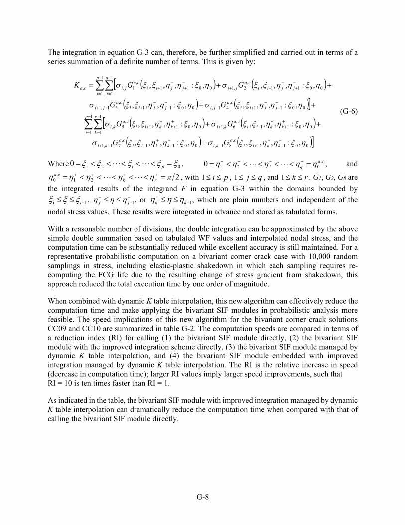
G-8

The integration in equation G-3 can, therefore, be further simplified and carried out in terms of a series summation of a definite number of terms. This is given by:

(G-6)

Where , , and

, with , , and . G1, G2, G8 are

the integrated results of the integrand F in equation G-3 within the domains bounded by

, , or , which are plain numbers and independent of the

nodal stress values. These results were integrated in advance and stored as tabulated forms.

With a reasonable number of divisions, the double integration can be approximated by the above simple double summation based on tabulated WF values and interpolated nodal stress, and the computation time can be substantially reduced while excellent accuracy is still maintained. For a representative probabilistic computation on a bivariant corner crack case with 10,000 random samplings in stress, including elastic-plastic shakedown in which each sampling requires re-computing the FCG life due to the resulting change of stress gradient from shakedown, this approach reduced the total execution time by one order of magnitude.

When combined with dynamic K table interpolation, this new algorithm can effectively reduce the computation time and make applying the bivariant SIF modules in probabilistic analysis more feasible. The speed implications of this new algorithm for the bivariant corner crack solutions CC09 and CC10 are summarized in table G-2. The computation speeds are compared in terms of a reduction index (RI) for calling (1) the bivariant SIF module directly, (2) the bivariant SIF module with the improved integration scheme directly, (3) the bivariant SIF module managed by dynamic K table interpolation, and (4) the bivariant SIF module embedded with improved integration managed by dynamic K table interpolation. The RI is the relative increase in speed (decrease in computation time); larger RI values imply larger speed improvements, such that RI = 10 is ten times faster than RI = 1.

As indicated in the table, the bivariant SIF module with improved integration managed by dynamic K table interpolation can dramatically reduce the computation time when compared with that of calling the bivariant SIF module directly.

0011

,81,0011

,71,1

1

1

1

10011

,6,10011

,5,

0011,

41,0011,

31,1

1

1

1

10011

,2,10011

,1,,

,:,,,,:,,,

,:,,,,:,,,

,:,,,,:,,,

,:,,,,:,,,

kkiica

kikkiica

ki

p

i

r

kkkii

cakikkii

caki

jjiica

jijjiica

ji

p

i

q

jjjii

cajijjii

cajica

GG

GG

GG

GGK

0210 pi caqj

,0210

221,

0 rk

ca pi 1 qj 1 rk 1

1i i

1jj

1kk

G-9

Table G-2. Comparison of computation times for calling the bivariant SIF module CC10 with and without the improved integration scheme and dynamic K table integration

Dynamic K Table Interpolation

Improved Integration Scheme Reduction Index

No No 1

Yes No 24

No Yes 15

Yes Yes 356

G.4 PRE-INTEGRATION METHODS FOR UNIVARIANT SIF SOLUTIONS

Current DARWIN univariant SIF solutions for cracks with 2 or 3 degrees of freedom use the WFs originally proposed by Shen and Glinka [G-4]. The SIF solutions are determined by integrating the product of the WF and the stress component normal to the crack plane across the specified crack depth. The selected WF depends on the location of the crack tip (surface tip or deepest tip).

The integration is performed in one dimension with a direction along the crack depth and currently is determined using the Gauss-Chebyshev numerical method with iterative convergence check. However, the iterative process associated with the numerical integration for convergence can become time consuming for steep stress gradients. Therefore, a new pre-integration method was developed to more efficiently evaluate the SIF.

The essence of this pre-integration scheme is to approximate the stress variation between user-specified stress values by Hermite polynomials and to break down the entire integration into one single pass of simple summation such that no further iteration is necessary. The computation time therefore becomes consistent and does not depend on the stress gradient, whereas the results are almost identical with the current numerically integrated results (note that a linear variation between user-specified stress values is assumed in the current version).

The formulation makes use of the following integral equations for SIF solutions in which is the variation of stress component normal to the crack, Wa and Wc denote Shen-Glinka WFs, and the SIF solutions are Ka and Kc where the subscripts a and c designate the crack tip locations the deepest tip and the surface tip, respectively.

(G-7)

The expansion of the integrand was derived based on the Glinka WF and the Hermite polynomial approximation of stress variation. The Shen-Glinka WFs are three terms of series expansion with

respect to the crack tip singularity (i.e., at a-tip and at c-tip respectively) and are given by:

a

cca

a

a dxx:aWxK,dxx:aWxK00

xa 1 x1

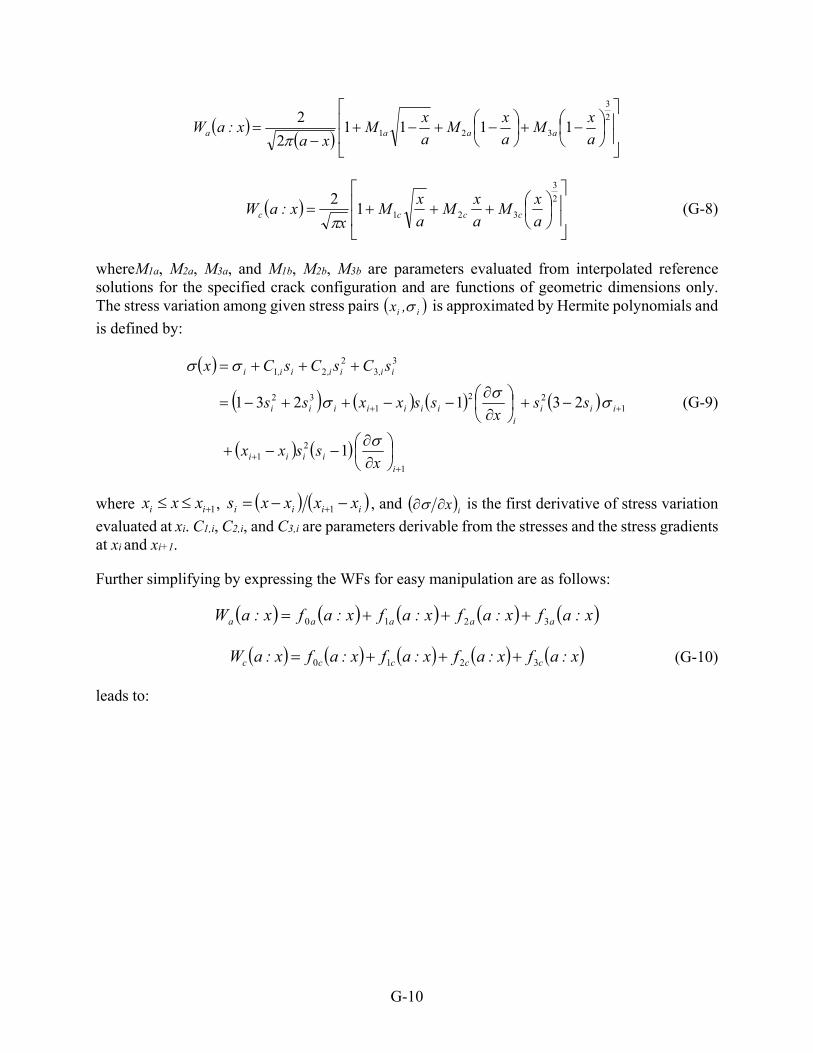
G-10

(G-8)

whereM1a, M2a, M3a, and M1b, M2b, M3b are parameters evaluated from interpolated reference solutions for the specified crack configuration and are functions of geometric dimensions only. The stress variation among given stress pairs is approximated by Hermite polynomials and

is defined by:

(G-9)

where , , and is the first derivative of stress variation

evaluated at xi. C1,i, C2,i, and C3,i are parameters derivable from the stresses and the stress gradients at xi and xi+1.

Further simplifying by expressing the WFs for easy manipulation are as follows:

(G-10)

leads to:

2

3

321 11112

2

a

xM

a

xM

a

xM

xax:aW aaaa

2

3

32112

a

xM

a

xM

a

xM

xx:aW cccc

ii ,x

1

21

122

132

33

221

1

231 231

iiiii

iiii

iiiiiii

ii,ii,ii,i

xssxx

ssx

ssxxss

sCsCsCx

1 ii xxx iiii xxxxs 1 ix

x:afx:afx:afx:afx:aW aaaaa 3210

x:afx:afx:afx:afx:aW ccccc 3210

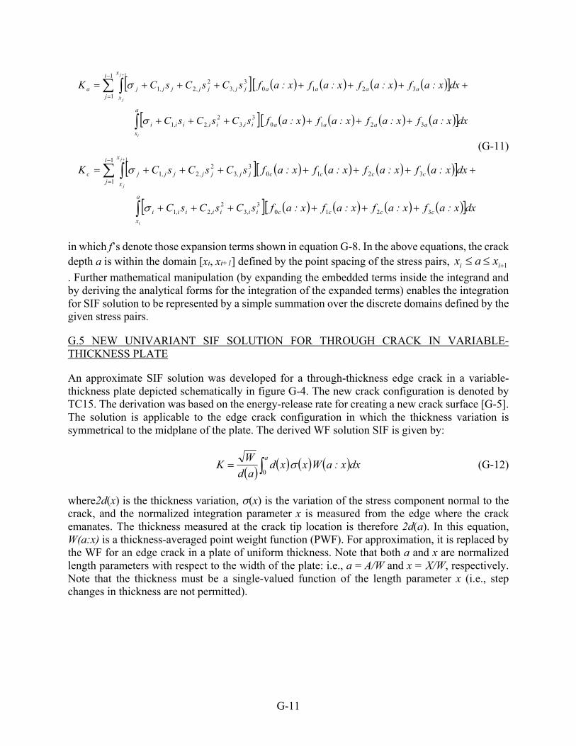
G-11

(G-11)

in which f’s denote those expansion terms shown in equation G-8. In the above equations, the crack depth a is within the domain [xi, xi+1] defined by the point spacing of the stress pairs,

. Further mathematical manipulation (by expanding the embedded terms inside the integrand and by deriving the analytical forms for the integration of the expanded terms) enables the integration for SIF solution to be represented by a simple summation over the discrete domains defined by the given stress pairs.

G.5 NEW UNIVARIANT SIF SOLUTION FOR THROUGH CRACK IN VARIABLE-THICKNESS PLATE

An approximate SIF solution was developed for a through-thickness edge crack in a variable-thickness plate depicted schematically in figure G-4. The new crack configuration is denoted by TC15. The derivation was based on the energy-release rate for creating a new crack surface [G-5]. The solution is applicable to the edge crack configuration in which the thickness variation is symmetrical to the midplane of the plate. The derived WF solution SIF is given by:

(G-12)

where2d(x) is the thickness variation, (x) is the variation of the stress component normal to the crack, and the normalized integration parameter x is measured from the edge where the crack emanates. The thickness measured at the crack tip location is therefore 2d(a). In this equation, W(a:x) is a thickness-averaged point weight function (PWF). For approximation, it is replaced by the WF for an edge crack in a plate of uniform thickness. Note that both a and x are normalized length parameters with respect to the width of the plate: i.e., a = A/W and x = X/W, respectively. Note that the thickness must be a single-valued function of the length parameter x (i.e., step changes in thickness are not permitted).

dxx:afx:afx:afx:afsCsCsC

dxx:afx:afx:afx:afsCsCsCK

aaaa

a

x

ii,ii,ii,i

aaaa

i

j

x

x

jj,jj,jj,ja

i

j

j

32103

32

21

3210

1

1

33

221

1

dxx:afx:afx:afx:afsCsCsC

dxx:afx:afx:afx:afsCsCsCK

cccc

a

x

ii,ii,ii,i

cccc

i

j

x

x

jj,jj,jj,jc

i

j

j

32103

32

21

3210

1

1

33

221

1

1 ii xax

dxx:aWxxdad

WK

a

0

G-12

(a) (b)

Figure G-4. Applicable cracked configuration for TC15 a through-thickness crack at the edge of a variable-thickness plate: (a) thickness variation across the plate section in

symmetry to the midplane of the plate and (b) remote ends subjected to loading normal to the crack

Given the following PWF for an edge crack in a plate of uniform thickness:

(G-13)

the integration for SIF solutions can be carried out numerically where the parameters i are interpolated from tables based on a given crack depth a.

Validation of this approximate solution has been performed against the results obtained using the 3D boundary element program, FADD3D. The numerical results for five different crack depths in a body with a linear-thickness variation were determined. The applied loading is remote tension. The linear variation of thickness is 1 + X/W, and the normalized crack depths in the comparison are 0.1, 0.2, 0.4, 0.6, and 0.8. Figure G-5 shows the boundary element model with the normalized crack length equal to 0.4. The comparison of the predicted results using the developed TC15 fracture mechanics module with the results from FADD3D is shown in figure G-6, and the two are in very good agreement.

X

2d(X)

A

W

A

W

S(X)

2

35

1

1 2

1

i

ii a

xa

a)x:a(W

G-13

Figure G-5. Boundary element model used for validating the TC15 SIF solution: the thickness variation is linear and given by 1+X/W; the normalized crack depth (a/w) shown

in the figure is 0.4, and the loading is remote tension

Figure G-6. Comparison of predicted results using the TC15 fracture mechanics module with FADD3D results: the continuous lines indicate the predicted results using the TC15

fracture mechanics modules, and the SIF results from FADD3D were taken at the intersection of the perimeter of the edge crack with the mid-plane of the plate

The pre-integration method described earlier was also applied to the integral equation for SIF solutions described in equation G-12 to break the integration into a simple summation over

A/W

0.0 0.2 0.4 0.6 0.8 1.0

No

rmal

ized

SIF

0

2

4

6

8

20304050

d(x)=1+X/Wd(x)=1FADD3D for d(x)=1+X/W

G-14

analytically derived terms. This derivation is applicable to the univariant WF solution for cracks with only 1 degree of freedom. The complication resulting from the variation in thickness (in addition to the stress variation), which leads to two sets of point spacing during integration, was resolved by introducing a dual indexing system. The indexing associates the integration bounds with the locations of data pairs defined in the thickness and stress variations, such that the integration domain of each interval can be clearly defined.

In this pre-integration method, both variations are assumed in their own point-spacing domains. The stress variation among the given stress pairs is expressed in terms of Hermite

polynomials given by:

(G-14)

where , , and is the first derivative of the stress

variation evaluated at xi. C1,i, C2,i, and C3,i are parameters derivable from the stresses and the stress gradients at xi and xi+1.

The thickness variation can be specified in two ways: either linearly interpolated or Hermite interpolated. Assuming the thickness pairs are given as , the linear variation is simply based

on the linear interpolation among data pairs defined by:

(G-15)

whereas the Hermite variation is in terms of Hermite polynomials and is given by:

(16)

where , , and is the first derivative of the thickness

variation evaluated at xj. D1,j, D2,j, and D3,j are parameters derivable from the thicknesses and the thickness gradients at xj and xj+1.

The analytical form can be derived after substituting the expansion forms for stress (see equation G-14), thickness (see equation G-15 or equation G-16), and WF (see equation G-8) into equation G-12, and the integration is then replaced by a simple summation over small intervals whose

ii ,x

1

21

122

132

33

221

1

231 231

iiiii

iiii

iiiiiii

ii,ii,ii,i

xssxx

ssx

ssxxss

sCsCsCx

1 ii xxx iiii xxxxs 1 ix

jj d,x

1 1 jjjj dtdtxd

1

21

122

132

33

221

1

231 231

jjjjj

jjjj

jjjjjjj

jj,jj,jj,j

x

dttxx

dttx

dttxxdtt

tDtDtDdxd

1 jj xxx jjjj xxxxt 1 jxd

G-15

domains are defined by the dual indexing system. In view of the lengthy expansion contributed by those functions, the details are excluded in this report.

A study of the relative computation speed was performed for four scenarios based on different combinations of point spacing and variations for thickness and stress, as described in table G-3. The thickness variation in Scenario I is linearly interpolated, in contrast to the thickness variation based on equally divided point spacing in Scenario II. Both scenarios use the Gauss-Chebychev numerical-integration scheme with convergence check to determine the SIF solutions. In contrast, Scenarios III and IV use the pre-integration method for the solutions. Note that the computation scheme used in Scenario II is the current method for univariant WF solutions in DARWIN. The applied stress gradient is mild (unit tension). The comparison indicates the pre-integration method can reduce the computation time by at least a factor of 2. For more pronounced gradients in both stress and thickness variations, the reduction in computation time is expected to be even more significant.

Table G-3. Study on the computation speed for four scenarios based on various combinations of specified point spacing in thickness and stress: the lower the RI, the faster

the computation speed.

Scenario Thickness Variation Stress Variation Execution Time for 1000 Loops RI

I Linear variation among thickness pairs

Equal point spacing 3 sec 37 ticks 2.46

II Equal point spacing Equal point spacing 3 sec 36 ticks 2.45

III* Linear variation among thickness pairs

Hermite variation among stress pairs

1 sec 37 ticks 1

IV* Hermite variation among thickness pairs

Hermite variation among stress pairs

1 sec 55 ticks 1.13

* For Scenarios III and IV, the pre-integration method was used.

G.6 NEW BIVARIANT AND UNIVARIANT SIF SOLUTIONS FOR ELLIPTICAL EMBEDDED CRACK IN PLATE

A new WF SIF solution for an elliptical embedded crack in a rectangular plate with a general bivariant stress field was also developed. This crack configuration is depicted in figure G-7. Previous DARWIN capabilities for embedded cracks (crack case EC02) addressed only univariant stress fields.

G-16

Figure G-7. Notations used for the embedded crack configuration in a rectangular section

G.6.1 REFERENCE SOLUTIONS

Reference solutions to support the WF method were generated using the new hybrid SGBEM-FEM (Symmetric Galerkin Boundary Element Method—Finite Element Method) feature in the FADD3D computer program [G-6], along with the commercial 3D computer-aided engineering software package, Patran, to develop the geometry models. This approach minimizes the problem size by isolating the complex modeling for the crack, especially along the crack perimeter, using surface boundary elements (BE) while replacing the neighboring domain by simple robust solid FEs. This feature is especially useful for generating reference solutions where repetitively adding or subtracting solid elements is required.

Figure G-8 shows a schematic of this approach in which solutions for different offsets can be modeled simply by modifying the required solid elements.

Figure G-8. How a hybrid FE/BE model (b) is composed of separate definitions (a) of FE solid elements, BE surface elements, BE interface and FE interface

Basic model components for this hybrid approach are (1) a BE submodel describing the crack and its immediate surrounding, (2) a node set containing the nodes along the interface of the BE

X

Y

x

y

Bt

Bw

b

T

W=2b

t=2T

a c

G-17

submodel with the FE submodel, (3) an FE submodel describing the remaining domain of the structure, and (4) a node set composed of the nodes along the interface of the FE submodel with the BE submodel. The specification of the interface between the BE submodel and the FE submodel is not required to be conforming (i.e., sharing the same nodal coordinates along the interface). However, if nonconforming interfacial conditions are used, attention must be given to minimizing the interaction of interfacial boundary and the crack surface by providing enough spacing in the boundary element model that contains the crack.

Modeling the entire structure using surface boundary elements is more straightforward and simple, but the pure BE approach results in a much larger problem size for the numerical computation. The hybrid approach is more balanced and practical: the global problem size is minimized by downplaying the contribution of the BE submodel and maximizing the usage of the FE submodel, reducing the turnaround time for generating large numbers of reference solutions.

The dimensionless parameters used for generating reference solutions for the embedded crack configuration are Bt/T, Bw/b, a/(TBt), c/(bBw), and a/c. These dimensional variables are defined in figure G-7. The discrete values of each parameter for the reference solution matrix are listed in table G-4. Accounting for symmetry conditions, the total number of geometry models required was 510. Because each model must be evaluated with three reference stresses, the total number of required computations becomes 1530. Only the embedded crack configuration in the first quadrant is considered. Results for cracks in the other three quadrants can be obtained through the conditions of symmetry.

Table G-4. Dimensionless parameter values evaluated for embedded crack reference solutions

Bt/T = 0, 0.5, 0.8

Bw/b = 0, 0.5, 0.8

a/(TBt) = 0.1, 0.4, 0.75, 0.99

c/(bBw) = 0.1, 0.4, 0.75, 0.99

a/c = 0.1, 0.3, 0.7, 1.0, 1.429, 3.333, 10.0

The maximum offset of the crack center, 80%, along both the x- and y-axes is determined by the observed behavior shown in figure G-9. The results indicate that, by keeping the other dimensionless parameters unchanged except the offset along the x-axis, the SIF variation along the embedded crack perimeter becomes stabilized once the offset of the crack center is approximately larger than 80%. In other words, the effect of the offset becomes minimal once the crack center is located more than 80% from the plate center. The maximum crack depth depends on the mesh densities. In this investigation, consistent mesh densities were used such that convergent results can be obtained for crack depth up to 99% of the net section.

G-18

Figure G-9. Variations of SIF along the embedded crack perimeter for various crack offsets indicate that the effect of the crack offset becomes minimal once the offset exceeds

approximately 80%; these results are based on c/(bBw)=0.9, a/(TBt)=0.9, a/c=1, and Bt/T=0, and the embedded crack is subjected to remote unit tension

Mesh densities in the numerical models can be evaluated by comparing their results with available analytical results. For embedded cracks in a comparatively large or pseudo-infinite domain, the analytical results by Shah and Kobayashi [G-7] for an embedded crack subjected to remote stress described by a polynomial function of up to the 3rd order were used. Figure G-10 shows the comparison in which three different stress variations were considered to account for any potential interaction between mesh density and stress variation. The graphs show the variations of normalized SIF along the embedded crack perimeter designated by the elliptical angle varying from 0 to 2 in reference to the local x-axis with the crack tip designation as: c-tip at =0, a-tip at =/2, c1-tip at =, and a1-tip at =3/2. The normalized SIF is with respect to the crack depth a and is given by where is the shape factor for an ellipse. In this configuration, the BE size

on the structure surface is relatively insensitive to the element size for the crack front. As shown, the two results are in excellent agreement.

2/

0 1 2 3 4

No

rmal

ized

SIF

1.1

1.2

1.3

1.4

1.5

1.6

1.7

1.8

Bw/b=0

Bw/b=0.5

Bw/b=0.833

Bw/b=0.9

a

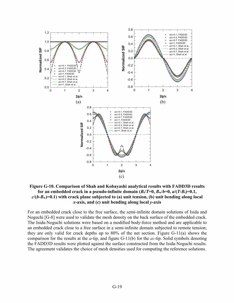
G-19

(a) (b)

(c)

Figure G-10. Comparison of Shah and Kobayashi analytical results with FADD3D results for an embedded crack in a pseudo-infinite domain (Bt/T=0, Bw/b=0, a/(T-Bt)=0.1,

c/(b-Bw)=0.1) with crack plane subjected to (a) unit tension, (b) unit bending along local x-axis, and (c) unit bending along local y-axis

For an embedded crack close to the free surface, the semi-infinite domain solutions of Isida and Noguchi [G-8] were used to validate the mesh density on the back surface of the embedded crack. The Isida-Noguchi solutions were based on a modified body-force method and are applicable to an embedded crack close to a free surface in a semi-infinite domain subjected to remote tension; they are only valid for crack depths up to 80% of the net section. Figure G-11(a) shows the comparison for the results at the a-tip, and figure G-11(b) for the a1-tip. Solid symbols denoting the FADD3D results were plotted against the surface constructed from the Isida-Noguchi results. The agreement validates the choice of mesh densities used for computing the reference solutions.

2/

0 1 2 3 4

No

rmal

ized

SIF

0.0

0.2

0.4

0.6

0.8

1.0

1.2

a/c=0.1, FADD3Da/c=0.3, FADD3Da/c=0.7, FADD3Da/c=1, FADD3Da/c=0.1, Shah et al.a/c=0.3, Shah et al.a/c=0.7, Shah et al.a/c=1, Shah et al.

2/

0 1 2 3 4

No

rmal

ized

SIF

-0.8

-0.6

-0.4

-0.2

0.0

0.2

0.4

0.6

0.8

a/c=0.1, FADD3Da/c=0.3, FADD3Da/c=0.7, FADD3Da/c=1, FADD3Da/c=0.1, Shah et al.a/c=0.3, Shah et al.a/c=0.7, Shah et al.a/c=1, Shah et al.

2/

0 1 2 3 4

No

rmal

ized

SIF

-0.8

-0.6

-0.4

-0.2

0.0

0.2

0.4

0.6

0.8a/c=0.1, FADD3Da/c=0.3, FADD3Da/c=0.7, FADD3Da/c=1, FADD3Da/c=0.1, Shah et al.a/c=0.3, Shah et al.a/c=0.7, Shah et al.a/c=1, Shah et al.

G-20

(a) (b)

Figure G-11. Comparison of computed FADD3D results (solid symbols) with Isida-Noguchi semi-infinite domain solutions (surface) for validating the mesh density used on the back

surface of an embedded crack close to a free surface. The stressing is a unit tension applied remotely. The graphs show the variations of normalized SIF as a function of dimensionless crack aspect ratio a/c and crack depth a/(TBt) for (a) a-tip and (b) a1-tip. Note the Isida-

Noguchi solutions are valid for crack depths up to 80% of the net section.

G.6.2 BIVARIANT WF SIF FORMULATION FOR EMBEDDED CRACK (EC04)

The PWF proposed by Orynyak and Borodii [G-9] for an embedded crack in an infinite domain is used as an approximate PWF and is given by:

(G-17)

This PWF represents the weighting effect of the applied unit point load at Q on a location Q’ along the crack perimeter (see figure G-12). The notation R denotes the distance between QR and Q*, r is the distance between Q and Q*, and the distance between Q and Q’.

0.6

0.8

1.0

1.2

1.4

0.00.2

0.40.6

0.8 0.00.2

0.40.6

0.81.0

No

rma

lize

d S

IF

a/(T-Bt)

a/c

0.6

0.8

1.0

1.2

1.4

0.00.2

0.40.6

0.8 0.00.2

0.40.6

0.81.0

No

rma

lized

SIF

a/(T-Bt)

a/c

2

22

'QQR

rRW

'QQ

G-21

Figure G-12. Embedded crack in an infinite domain

The approximate nature of this PWF can be demonstrated by comparing the infinite-domain solutions with the integrated results over the entire crack surface area using equation G-17 as a basic PWF; they do not converge together. Therefore, a PWF that includes three correction terms was postulated to account for the effects of free surfaces. The functional form is given by:

(G-18)

where Wcorrection represents the correction terms with coefficients 1, 2, and 3, and Q(x,y) denotes the location where the point load is applied. The chord lengths x’ and y’ at (x,y) can be determined by:

(G-19)

SIGN(Q’,y) denotes the sign of the x-coordinate of Q’ and SIGN(Q’,x) the sign of the y-coordinate of Q’. The SIF for any location Q’ along the crack perimeter can thus be written as:

(G-20)

where the integration is carried out over the entire embedded crack surface.

The surface integral can be written in terms of an elliptical coordinate system with its origin at the crack center to facilitate further mathematical manipulations. In that case, Q*, Q and QR are defined to share the same elliptical angle , and Q’ and QR have the same elliptical “radius” 0. The value of 0 depends on the crack aspect ratio = a/c. For a/c < 1 and ,

x

y

QR(0, )

Q(, )

Q*(0, )

Q’(0, 0) a

c

'xx,'QSIGN

x

'yy,'QSIGN

y

R

r

R

rR

WWW

'QQ

correctionbasic

1111 3212

22

2

2

2

2

1 , 1c

xa'y

a

yc'x

A

'Q dAy,xWK

22 acb

G-22

(G-21)

(G-22)

(G-23)

(G-24)

(G-25)

(G-26)

(G-27)

and the integral becomes

(G-28)

The coefficients 1, 2, and 3 are determined by three sets of reference solutions at the preferred crack-tip locations. The surface integral can be determined by the Gauss-Chebyshev numerical integration scheme. To further reduce the computational efforts associated with the numerical integration and convergence check, the pre-integration method for bivariant SIF solutions documented earlier was used.

Severe local stress gradients applied on the crack surface were used to validate the bivariant WF formulation for EC04. Mainly they were local stressing: (x,y) = (1x2/c2)/(1y2/a2), (1x3/c3)/(1y3/a3), and (1x4/c4)/(1y4/a4), where both x and y are in reference to the local coordinate system fixed to the crack center. These stress distributions can be nonsymmetrical. Figure G-13 shows the comparison of predicted results using EC04 with independent FADD3D results when the embedded crack is in the plate center and has a severe crack aspect ratio: Bt/T = Bw/b = 0, a/T = 0.99, c/b = 0.99, and a/c = 0.1. Figure G-13(a) shows the SIF variation along the crack perimeter from FADD3D and the discrete results at crack tips by EC04. Here, the SIF variation was plotted from the c-tip ( = 0) to c1-tip (= ) and then back to the same c-tip (=2), counterclockwise. The symmetrical variation results from the conditions of symmetry exhibited in both cracked geometry and stressing. The symmetrical variation breaks down when the applied stressing is nonsymmetrical, as indicated in figure G-13(b).

Figure G-14 depicts the comparison when the embedded crack is 80% offset from the plate center: Bt/T = Bw/b = 0.8, a/T = 0.99, c/b = 0.99, and a/c = 0.1. Comparing figures G-13(b) and G-14(a) shows that although the weighting of stress variation tends to increase the SIF values in the 3rd and 4th quadrants, as indicated in figure G-13, the offset of the crack brings in the free surface effect, and inevitably the SIF results in the 1st and 2nd quadrants become dominant and overshadow other

sinsinhbycoscoshbx ,

1

10 ln

20

220 sinsinhcoscoscoshbR

222 sinsinhcoscoscoshbr

200

200 sinsinhsinsinhcoscoshcoscoshb'QQ

22

0222

02

, sinsinhsinh

coscosh

'x

x

coscoshcosh

sinsinh

'y

y

ddsinhsinbdA 222

ddsinhsinc,WWK correctionbasic'Q 222

0

2

0

0

G-23

quadrants. Note that the results shown in figures G-13(b) and G-14(a) were based on the same applied stresses.

These validation plots show that the SIF variations among four crack tips can be extremely nonlinear and complex under severe stressing with highly skewed crack aspect ratios. Nevertheless, the proposed EC04 WF formulation is capable of accurately capturing these key features in SIF variations and is in good agreement with the computed results using FADD3D.

(a) (b)

Figure G-13. The comparison of the predicted results using EC04 and independent computed results from FADD3D: (a) (x,y) = (1x2/c2)/(1y2/a2) and (b) (x,y) =

(1x3/c3)/(1y3/a3); the dimensionless geometric parameters are Bt/T = Bw/b = 0, a/T = 0.99, c/b = 0.99, and a/c = 0.1

2

0 1 2 3 4

No

rmal

ized

SIF

, K/[(a

)]

-1

0

1

2

3

4

FADD3DEC04

2

0 1 2 3 4

No

rmal

ized

SIF

, K

/[

( a)

]

-2

0

2

4

6

8

FADD3DEC04

G-24

(a) (b)

Figure G-14. The comparison of the predicted results using EC04 and independent computed results from FADD3D: (a) (x,y) = (1x3/c3)/(1y3/a3) and (b) (x,y) =

(1x4/c4)/(1y4/a4); the dimensionless geometric parameters are Bt/T = Bw/b = 0.8, a/T = 0.99, c/b = 0.99, and a/c = 0.1

G.6.3 UNIVARIANT WF SIF FORMULATION FOR EMBEDDED CRACK (EC05)

Although a univariant WF SIF solution for an embedded crack in a plate (EC02) was already available in DARWIN, a new univariant solution (EC05) was developed so that it would be fully consistent with the new bivariant solution EC04 for cases in which the stress gradient was strictly univariant. This new univariant solution employed an appropriate subset of the same reference solutions as EC04. The formulation of the univariant solution is summarized below.

The PWF was derived based on the assumption that the stress distribution varies in one direction, along the local y-axis. In reference to figure G-15, the 1D basic WF varying along the y-axis for a-, c-, a1- and c1-tips can be determined by integrating the PWF for a penny-shape embedded crack in an infinite domain with a unit load along the chord perpendicular to the y-axis. By preserving the singular terms in the basic WFs and on account of two sets of reference solutions, the approximate 1D WFs were postulated as:

2

0 1 2 3 4

No

rmal

ized

SIF

, K/[

( a)

]

0.0

0.5

1.0

1.5

2.0

2.5

3.0

FADD3DEC04

2

0 1 2 3 4

No

rmal

ized

SIF

, K/[

( a)

]

0.0

0.5

1.0

1.5

2.0

2.5

FADD3DEC04

G-25

Figure G-15. Embedded crack subjected to univariant stressing along local y-axis

(G-29)

(G-30)

(G-31)

The M’s are the coefficients for correction terms and the WF solutions for a-, a1- and c-tips (or c1-tip) are given by:

(G-32)

(G-33)

(G-34)

These coefficients can be determined by boundary conditions and reference solutions. For the a-tip, they are given by:

(G-35)

x

y(y)a

c1 c

a1

x

y(y)a

c1 c

a1

23

321 11112

2

a

yM

a

yM

a

yM

yayW aaaa

23

321 11112

2111

a

yM

a

yM

a

yM

yayW aaaaa

0 if1

1

0 if11

21

21

1

ya

yM

a

yM

y

ya

yM

a

yM

yyWyW

cc

cc

cc

a

a

aaaa dya

yM

a

yM

a

yM

ya

yK

23

321 11112

2

a

a

aaa

a

a

aaaa

dya

yM

a

yM

a

yM

ya

y

dya

yM

a

yM

a

yM

ya

yK

23

321

23

321

11112

2

11112

2

111

1111

dy

a

yM

a

yM

y

yyKK

a cccc

0 2111

ab

au

a K~

QK~

QM

22

15

22

3241

G-26

(G-36)

(G-37)

where and are the normalized reference solutions of and by and Q is the

shape factor for an ellipse. Using a similar approach, the other coefficients can be determined.

Extensive validation has been completed by comparing the computed EC05 results against the results from the older EC02 module and from independent boundary element results using FADD3D. The selective geometric combinations used for validation were:

Bt/T = Bw/b = 0, 0.8

a/(TBt) = c/(bBw) = 0.1, 0.75, 0.99

a/c = 0.1, 0.3, 0.7 1.0

Selective comparison results shown in figure G-16 have the applied stress defined by (y) = (y/a)2. EC05 is in excellent agreement with the FADD3D solutions and (for most cracks) with the EC02 solutions. The largest disagreements between EC02 and the FADD3D results correspond to a/(TBt) = c/(bBw) = 0.99 and a/c = 0.1 and 0.3. This is expected because the EC02 module is not strictly valid for crack depths more than 80% of the net section. However, it should be noted that these errors in EC02 would not generally introduce significant error in FCG lifetime calculations because most of the lifetime is generally consumed when the crack is small compared to the net section. Comparisons of FCG lifetimes and crack aspect ratios between EC05 and EC02 (not shown here) indicated excellent agreement in most cases. Therefore, it is not currently anticipated that replacement of EC02 by EC05 will introduce significant changes in calculated life or risk. However, EC05 should give more accurate answers in some situations, and the answers will be consistent with EC04 for univariant stress fields.

A comparison between EC05 and the old EC03 solution for an embedded crack approaching a free surface can be found in figure G-17. Here the applied stress on the crack plane is uniform tension. The EC05 results are in excellent agreement with the original results by Isida and Noguchi [G-8] on which EC03 was based, while the EC03 results show a small discrepancy at the a1-tip for small crack depths (a/(TBt)0) when the crack aspect ratio approaches a semi-ellipse (a/c1).

ab

au

a K~

QK~

QM

4

45

4

15

2

152

ab

au

a K~

QK~

QM

22

15

23223

auK

~ abK

~ auK a

bK Qa

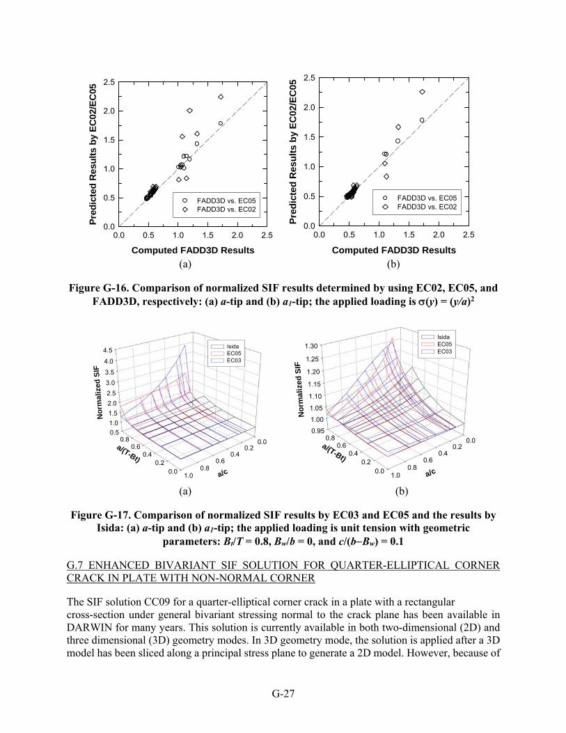
G-27

(a) (b)

Figure G-16. Comparison of normalized SIF results determined by using EC02, EC05, and FADD3D, respectively: (a) a-tip and (b) a1-tip; the applied loading is (y) = (y/a)2

(a) (b)

Figure G-17. Comparison of normalized SIF results by EC03 and EC05 and the results by Isida: (a) a-tip and (b) a1-tip; the applied loading is unit tension with geometric

parameters: Bt/T = 0.8, Bw/b = 0, and c/(bBw) = 0.1

G.7 ENHANCED BIVARIANT SIF SOLUTION FOR QUARTER-ELLIPTICAL CORNER CRACK IN PLATE WITH NON-NORMAL CORNER

The SIF solution CC09 for a quarter-elliptical corner crack in a plate with a rectangular cross-section under general bivariant stressing normal to the crack plane has been available in DARWIN for many years. This solution is currently available in both two-dimensional (2D) and three dimensional (3D) geometry modes. In 3D geometry mode, the solution is applied after a 3D model has been sliced along a principal stress plane to generate a 2D model. However, because of

Computed FADD3D Results

0.0 0.5 1.0 1.5 2.0 2.5

Pre

dic

ted

Res

ult

s b

y E

C02

/EC

05

0.0

0.5

1.0

1.5

2.0

2.5

FADD3D vs. EC05FADD3D vs. EC02

Computed FADD3D Results

0.0 0.5 1.0 1.5 2.0 2.5

Pre

dic

ted

Res

ult

s b

y E

C02

/EC

05

0.0

0.5

1.0

1.5

2.0

2.5

FADD3D vs. EC05FADD3D vs. EC02

0.5

1.0

1.5

2.0

2.5

3.0

3.5

4.0

4.5

0.00.2

0.40.6

0.8 0.00.2

0.40.6

0.81.0

No

rmal

ized

SIF

a/(T-Bt)

a/c

IsidaEC05EC03

0.95

1.00

1.05

1.10

1.15

1.20

1.25

1.30

0.00.2

0.40.6

0.8 0.00.2

0.40.6

0.81.0

No

rmal

ized

SIF

a/(T-Bt)

a/c

IsidaEC05EC03

G-28

modeling round-off errors, the resulting corner angle in the 2D slice model is sometimes not exactly perpendicular. In the past, this meant that the CC09 solution could not be applied because the bivariant WF integration schemes were based on a perpendicular corner angle. Therefore, it was desirable to enhance the CC09 solution to permit it to be applied to corner angles that deviated slightly from 90 degrees. In this enhanced version, the maximum permissible angular variation of the corner from 90 is 5.

The nonrectangular cross section supported by the enhanced CC09 solution is depicted in figure G-18. The initial corner crack site resides at the bottom left corner, which is designated as the first included angle of the cross-section. The remaining included angles are denoted in clockwise order for a unique definition of plate cross-section. By this definition, the second and third angles are 90, and the last/fourth angle is supplemental to the first angle. The nomenclature used in the original DARWIN CC09 crack type for plate thickness and width, and crack depth and width, has been slightly changed, as shown in figure G-18. The dimensions are in reference to the crack origin: the plate width and thickness, hy and hy, are the projected lengths to the side surfaces, and the crack depth and width, a and c, are measured along the surfaces defining the corner.

The definition for the crack-tip perimeter remains consistent with those in the rest of DARWIN crack models. The governing equation is for describing an ellipse (i.e., the elliptical shape is not assumed to be distorted because of the non-perpendicular corner). So, it can be envisioned that for a very small crack shape aspect ratio (small a/c ratio), there could be controversies regarding the proper definition of c-tip and the validity of its SIF solution at the location where the crack tip perimeter intersects with the free surface near an 85 or 95 corner. This particular configuration is unlikely to occur in practice, but the reference solutions must still be generated to facilitate interpolation within the reference solution array.

The stress fields used to generate the reference stress solutions are the same as those used in the original CC09 development: one tensile and two bending stress variations applied separately on the crack surface. They are defined in reference to the coordinate axes. Respectively, they are

given by , , and , where the parameters a and b define the

elliptical crack tip perimeter: . Note that the SC length c is the surface breaking line defined by the intersection of the crack-tip perimeter and the free surface, and this line may not be along the y-axis (see again figure G-18). The maximum permissible angular variation in this enhanced solution was defined to be 5 from the 90 corner.

1 1 2 1 ⁄ 2 1 2

2 2

2 1

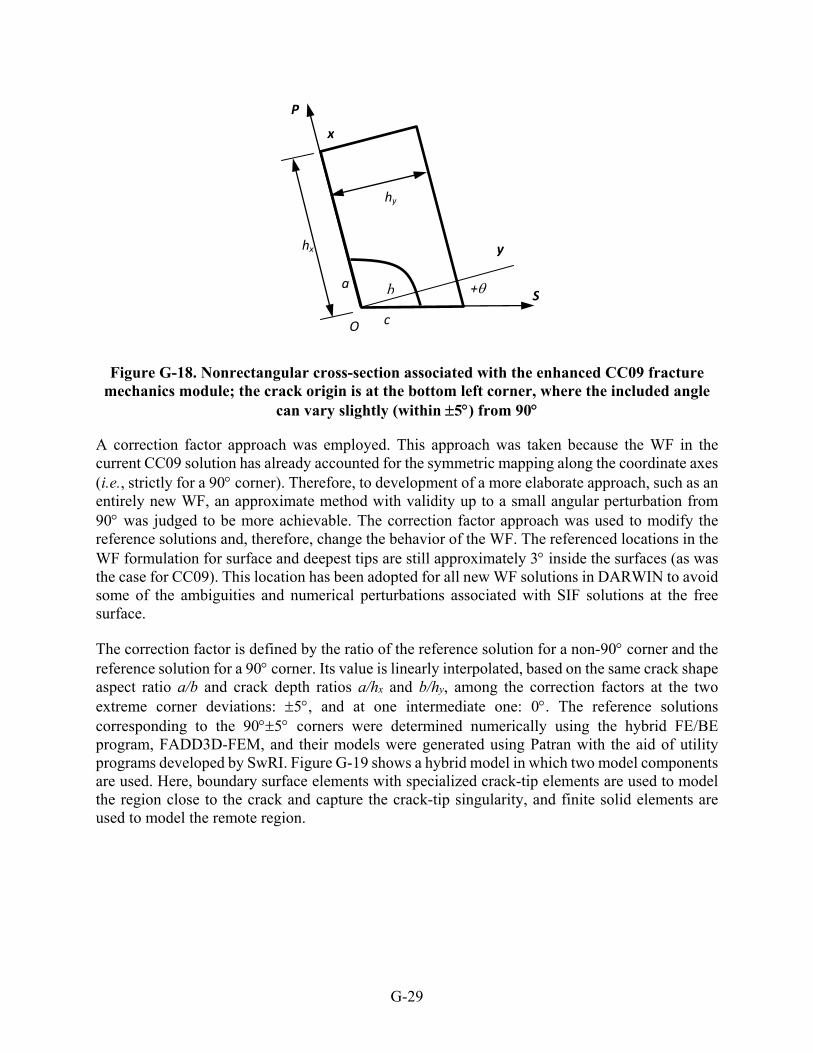
G-29

Figure G-18. Nonrectangular cross-section associated with the enhanced CC09 fracture mechanics module; the crack origin is at the bottom left corner, where the included angle

can vary slightly (within 5) from 90

A correction factor approach was employed. This approach was taken because the WF in the current CC09 solution has already accounted for the symmetric mapping along the coordinate axes (i.e., strictly for a 90 corner). Therefore, to development of a more elaborate approach, such as an entirely new WF, an approximate method with validity up to a small angular perturbation from 90 was judged to be more achievable. The correction factor approach was used to modify the reference solutions and, therefore, change the behavior of the WF. The referenced locations in the WF formulation for surface and deepest tips are still approximately 3 inside the surfaces (as was the case for CC09). This location has been adopted for all new WF solutions in DARWIN to avoid some of the ambiguities and numerical perturbations associated with SIF solutions at the free surface.

The correction factor is defined by the ratio of the reference solution for a non-90 corner and the reference solution for a 90 corner. Its value is linearly interpolated, based on the same crack shape aspect ratio a/b and crack depth ratios a/hx and b/hy, among the correction factors at the two extreme corner deviations: 5, and at one intermediate one: 0. The reference solutions corresponding to the 905 corners were determined numerically using the hybrid FE/BE program, FADD3D-FEM, and their models were generated using Patran with the aid of utility programs developed by SwRI. Figure G-19 shows a hybrid model in which two model components are used. Here, boundary surface elements with specialized crack-tip elements are used to model the region close to the crack and capture the crack-tip singularity, and finite solid elements are used to model the remote region.

  P 

S 

O 

hy 

hx 

+ a 

c 

x 

y 

b

G-30

Figure G-19. Hybrid model consisting of boundary surface elements and finite solid elements for modeling a crack with small crack shape aspect ratio at an 85 corner;

boundary surface elements are used close to the cracked region to better capture the salient features of the crack tip singularity

Figure G-20 shows the crack shapes that result from a small aspect ratio (a/b=0.1) when the included angle of the corner varies from 85 to 95. Both cracks have the same crack-depth ratios. Figure G-20(a) shows the crack shape for an 85 corner, and figure G-20(b) shows the crack shape for a 95 corner. Both shapes lead to a sharp nonperpendicular tri-surface geometric intersection at the c-tip. The SIF variation close to the c-tip in figure G-20(b) can therefore be expected to vary abruptly, resulting from the reduced ligament between the local curvature of the crack-tip perimeter and the free surface. This also indicates the proposed approximate procedure may have some difficulty capturing the salient SIF behavior at the c-tip for small crack shape aspect ratios with these two extreme corner variations. For a crack with a large crack shape aspect ratio, it becomes less of a problem because of the smoother curvature of the crack-tip perimeter at the c-tip and its tendency of the angle at the free surface to approach perpendicularity.

FE Section

FE Section

BE Section

Crack

G-31

Figure G-20. Comparison of crack tip perimeter for corner crack with small crack shape

aspect ratio (a) at an 85 corner and (b) at a 95 corner; both result in a sharp nonperpendicular tri-surface geometric intersection at the c-tip

The resulting SIF solutions vary around the crack-tip perimeter. Figure G-21 shows the results for one specific crack geometry (a/b = 1, a/hx= 0.9 and b/hy = 0.5) as a function of the normalized elliptical angle 2/ for three different corner angles (85, 90, and 95). In these plots, a 95 corner leads to the elliptical angle, starting from a negative value, and an 85 corner, starting from a positive value. The SIF value at the c-tip is generally taken slightly larger than the starting elliptical angle (slightly inside the free surface). 2/ = 0 represents the crack tip location at the y-axis (b-tip), and 2/ = 1 denotes the crack tip location at the x-axis (a-tip). The SIF values are

normalized with respect to where is the shape factor for an ellipse.

Verification was performed by comparing SIF values from the modified CC09 SIF fracture mechanics module with those determined directly by FADD3D calculations. Three reference stresses were used to determine how well the correction factor approach works. Figures G-22 and G-23 show representative comparisons. Figure G-22 compares the SIF results of an 85 corner subjected to tensile reference stress for a variety of a/b, a/hx and b/hy combinations. Figure G-22(a) shows c-tip results, and figure G-22(b) shows a-tip results. Similar comparisons for a 95 corner subjected to reference bending stress with respect to the y-axis are shown in figure A-6, where figure G-23(a) shows c-tip results and figure G-23(b) shows a-tip results. Most of the comparisons exhibit good agreement based on the proposed correction factor approach.

(a) (b)

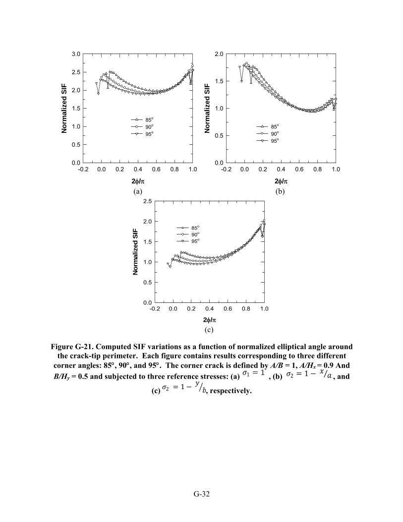
G-32

(a) (b)

(c)

Figure G-21. Computed SIF variations as a function of normalized elliptical angle around the crack-tip perimeter. Each figure contains results corresponding to three different

corner angles: 85, 90, and 95. The corner crack is defined by A/B = 1, A/Hx = 0.9 And

B/Hy = 0.5 and subjected to three reference stresses: (a) , (b) , and

(c) , respectively.

2/

-0.2 0.0 0.2 0.4 0.6 0.8 1.0

No

rmal

ize

d S

IF

0.0

0.5

1.0

1.5

2.0

2.5

3.0

85o

90o

95o

2/

-0.2 0.0 0.2 0.4 0.6 0.8 1.0

No

rmal

ize

d S

IF

0.0

0.5

1.0

1.5

2.0

85o

90o

95o

2/

-0.2 0.0 0.2 0.4 0.6 0.8 1.0

No

rmalize

d S

IF

0.0

0.5

1.0

1.5

2.0

2.5

85o

90o

95o

2 1 ⁄

2 1

G-33

(a) (b)

Figure G-22. Comparison of computed SIF results from the modified Cc09 with the reference solutions determined using FADD3D: (a) c-tip and (b) A-tip; the applied

reference stress is tensile and the included angle of the corner is 85

(a) (b)

Figure G-23. Comparison of computed SIF results from the modified Cc09 with the reference solutions determined using FADD3D: (a) c-tip and (b) A-tip; the applied

reference stress is bending along the y-axis and the included angle of the corner is 95

The problem mentioned earlier involving the c-tip arising from the interaction of the small crack shape aspect ratio at a non-90 corner angle does manifest itself. Figure G-24(a) shows the comparison of SIF results at the c-tip from the modified CC09 with the reference solutions using FADD3D for a crack at an 85 corner subjected to reference bending stress along the x-axis.

Normalized SIF by FADD3D

10-1 100 101

No

rmal

ized

SIF

by

CC

09

10-1

100

101

Normalized SIF by FADD3D

10-1 100 101

No

rmal

ized

SIF

by

CC

09

10-1

100

101

Normalized SIF by FADD3D

10-1 100 101

No

rmal

ized

SIF

by

CC

09

10-1

100

101

Normalized SIF by FADD3D

10-2 10-1 100 101

No

rmal

ized

SIF

by

CC

09

10-2

10-1

100

101

G-34

The data points noticeably above the one-to-one line are those with small crack shape aspect ratios. The comparison shows that the SIF results from the modified CC09 for smaller crack shape aspect ratios are conservative. The SIF results at the a-tip (shown in figure G-24(b)) do not exhibit such a problem.

(a) (b)

Figure G-24. Comparison of computed SIF results from the modified Cc09 with the reference solutions determined using FADD3D: (a) c-tip and (b) a-tip. The applied

reference stress is bending along the x-axis, and the included angle of the corner is 85

G.8 REFERENCES

G-1. FAA Report. (2008). Turbine Rotor Material Design—Phase II. (DOT/FAA/AR-07/13).

G-2. Lee, Y.-D., McClung, R.C., and Chell, G.G. (2008). An Efficient Stress Intensity Factor Solution Scheme for Corner Cracks at Holes under Bivariant Stressing. Fatigue and Fracture of Engineering Materials and Structures, 31(11) 1004–1016.

G-3. Li, S., Mear, M.E., and Xiao, L. (1998). Symmetric Weak-Form Integral Equation Method for Three-Dimensional Fracture Analysis. Computer Methods in Applied Mechanics and Engineering, 151(3–4) 435–539.

G-4. Shen, G., and Glinka, G. (1991). Weight Functions for a Surface Semi-Elliptical Crack in a Finite Thickness Plate. Theoretical and Applied Fracture Mechanics, 15(3) 247–255.

G-5. Akhurst, K. and Chell, G.G. (1983). Methods of Calculating Stress Intensity Factors for Nozzle Corner Cracks. International Journal of Pressure Vessels and Piping, 14(4), 227–257.

G-6. Rungamornrat, J. and Mear, M.E. (2011). SGBEM-FEM Coupling for Analysis of Cracks in 3D Anisotropic Media. International Journal for Numerical Methods in Engineering, 86(2), 224–248.

Normalized SIF by FADD3D

10-1 100 101

No

rmaliz

ed S

IF b

y C

C09

10-1

100

101

Normalized SIF by FADD3D

10-1 100 101N

orm

aliz

ed S

IF b

y C

C09

10-1

100

101

G-35

G-7. Shah, R.C. and Kobayashi, A.S. (1971). Stress Intensity Factor for an Elliptical Crack under Arbitrary Normal Loading. Engineering Fracture Mechanics, 3(1), 71–96.

G-8. Isida, M. and Noguchi, H. (1984). Tension of a Plate Containing an Embedded Elliptical Crack. Engineering Fracture Mechanics, 20(3), 387–408.

G-9. Orynyak, I. V. and Borodii, M.V. (1995). Point Weight Function Method Application for Semi-Elliptical Mode I Cracks. International Journal of Fracture, 70(2), 117–124.

H-1

APPENDIX H—ADAPTIVE RISK REFINEMENT

H.1 INTRODUCTION

Probabilistic fracture mechanics is a well-established approach to assess the probability of fracture (POF) of turbine engine rotor disks subjected to low-cycle fatigue [H-1, H-2]. This methodology uses a zone-based risk-integration scheme to account for the uncertainty of location of randomly distributed anomalies within a disk. A zone is a grouping of material that has a generally uniform stress state, similar fatigue crack-growth properties, inspection schedules, and distribution of anomalies. The risk contribution from each zone is based upon the life-limiting location to ensure a conservative risk solution.

The POF of a zone is given by:

(H-1)

where is the probability of an anomaly in zone i, and is the conditional POF given

an anomaly in zone i. The POF of the entire disk is the probability union of the zone risks:

(H-2)

where is the number of zones, and indicates fracture of an initial anomaly located in zone i.

The accuracy of the disk risk value is dependent upon the number of zones. A coarse discretization of zones yields a less accurate result compared to a fine one. The zone mesh is refined through an iterative process. Figure H-1 shows a sequence of the zone-refinement process for an example rotor disk in which the shaded regions indicate zones that require refinement. The need for refinement is based on the risk contribution factor (RCF) of a zone:

(H-3)

Zones are refined by manually partitioning the domain into two or four subzones for surface and embedded zones, respectively.

The zone-refinement process is a potentially time-consuming process that is performed by a human. Therefore, an adaptive risk refinement methodology (ARRM) was developed to reduce human involvement in the zone discretization process. ARRM includes an adaptive nodal selection feature designed to identify the optimal distribution of nodes on the surface of the component, and it employs constrained Delaunay triangulation (CDT) to connect the nodes into an initial mesh. ARRM numerically integrates the surface of the initial mesh to estimate the cumulative conditional POF. The initial mesh is repeatedly refined until a converged disk-risk solution is obtained.

][ iFP

]|[][][ iiii ABPAPFP

][ iAP ]|[ ii ABP

diskP

K

iiKdisk FPFFFPP

121 ])[1(1][

K iF

disk

ii P

FPRCF

][

H-2

Figure H-1. Sequence of the zone refinement process for a typical gas turbine engine rotor disk

H.2 BACKGROUND

For illustrative purposes, the POF associated with an impeller rotor-disk model (figure H-2(a)) was obtained using a large number of zones. The POF for each zone represents the conditional POF before 20,000 fatigue cycles, given an anomaly originating in that zone. The resulting conditional POF surface shown in figure H-2(b) serves as a benchmark for assessing the effectiveness of ARRM.

(a) (b)

Figure H-2. (a) Impeller rotor disk, and (b) benchmark conditional POF surface based on 1150 nodal coordinates at the life-limiting location of each

Development of a zone-discretization methodology focuses on the conditional POF in rotor disks. Conditional POF responses are high along edges associated with high stresses and abruptly diminish toward the interior of a disk. This generates steep gradients along rotor-disk edges, as shown in the benchmark impeller surface (figure H-2(b)). From a modeling perspective, the slope of the gradient

H-3

is the most important aspect of rotor-disk conditional POF behavior because it is difficult to develop a response surface for steep gradients.

Several methods were considered for modeling the conditional POF response, including ordinary K\kriging (OKR), multivariate adaptive regression splines (MARS), artificial neural networks (ANN), and polynomial regression (PR) [H-3 - H-7]. MARS and ANN are capable of modeling steep gradients associated with rotor disk conditional POF behavior. However, they require a substantially large number of training points, making them computationally expensive. A training point is a nodal response required by a metamodel to build a response surface from which the response at other coordinates can be estimated. PR fails to generate successful models because its data-smoothing nature inhibits it from characterizing abrupt response changes. OKR can model steep gradients using relatively few training points. However, as shown in figure H-3, the accuracy of the OKR model may actually decrease with an increase in the number of training points.

(a) (b)

Figure H-3. The accuracy of the ordinary kriging model may actually decrease with an increase in the number of training points: (a) 40 training points and (b) 50 training points

H.3 GENERATION OF INITIAL MESH

The initial mesh is based on the nodal coordinates of a finite element model (FEM). Mesh generation consists of three steps: (1) surface node selection, (2) embedded node selection, and (3) constrained Delaunay triangulation (CDT). Surface nodes are selected with the intention to accurately model conditional POF along a rotor disk surface using a minimal number of nodes.

10.1.1 H.3.1 Surface Node Selection

The surface node selection process begins with the identification of an initial nodal set. This set is defined as the coordinates of surface nodes located at gradient reversals along the delta stress response curve shown in figure H-4. The POF is predicted at each of the initial approach node locations using the critical defect size (CDS), where CDS is an efficient method for computing the conditional POF [H-1] (figure H-5). Not every member in the nodal set is needed to characterize the CDS response curve. Some nodes can be removed without a significant change in the response, as shown in figure H-6. The area under the estimated CDS curve differs less than 1% from the area under the estimated CDS curve in figure H-5. Estimated CDS curves are created by connecting neighboring nodes using one-dimensional linear elements.

H-4

Figure H-4. Nodal reduction of estimated CDS response curve

Figure H-5. Initial node set is based on stress gradient reversals along the surface of the disk

Figure H-6. The POF is predicted at each node using the CDS approach

The estimated CDS curve is refined through a process called curve refinement, whereby substandard elements are identified and subdivided. A substandard element is an element whose accuracy falls below a threshold value, which is selected depending upon the desired level of accuracy for the refined curve. Accuracy is quantified using the relative difference between the area underneath an element and the area under the actual CDS response curve encompassed by the element’s endpoints. The actual CDS response curve is unknown; therefore, an estimate of the actual curve’s area is used. It is obtained by computing the CDS response at an element’s bisection coordinate, subdividing the element at the bisection node, and computing the cumulative area underneath the resulting subelements. Substandard elements are replaced by their subelements. Figure H-7 shows the result of curve refinement applied to the estimated CDS response curve.

H-5

Figure H-7. Curve refinement improves the accuracy of the estimated CDS response curve

Again, the nodal set passes through the nodal-reduction process (figure H-8(a)). This concludes identification of the nodal set essential to the characterization of conditional POF along a rotor-disk surface. However, as shown in figure H-8(b), the nodal set does not address the rotor-disk geometric profile. Therefore, geometry-based nodes are appended to the response-based nodal set.

(a) (b)

Figure H-8. (a) Nodal reduction is applied a second time to the refined estimated CDS curve, and (b) response-based nodes plotted in 2D geometric plane fail to characterize rotor

disk geometry

Geometry-based nodes are obtained through skeletonization and geometric refinement. Skeletonization is a method that provides the thinnest representation of a geometric outline (skeleton) that preserves the topology. Although many skeletonization techniques exist [H-8–H-11], ARRM approximates rotor-disk skeletons by identifying the Voronoi diagram generated using the FEM surface nodes. The interior segments in the Voronoi diagram provide the rotor-disk skeleton. Figure H-9(a) is the Voronoi diagram of the impeller rotor disk, and figure H-9(b) shows the corresponding skeleton and its endpoints. The skeleton endpoints are important because they identify the apexes of geometric convexities within a rotor disk. Consequently, adding the nodal coordinates of the skeleton endpoints to the response-based nodal set creates an estimated surface model that encompasses the rotor disk. Figure H-10(a) shows the estimated model consisting of both the response-based nodes and skeleton endpoints.

H-6

To improve geometric accuracy, the estimated surface model is refined with respect to the rotor disk geometry using curve refinement. Element accuracy is assessed using the relative error between the length of an element and the length of the actual rotor-disk edge encompassed by the element’s endpoints. Substandard elements are determined by the relative-error threshold. A lower threshold results in a more accurate depiction of the rotor-disk geometry. Substandard elements are subdivided at the FEM surface node whose Euclidean distance to its relative location along the element is greatest. The process is repeated until all elements satisfy the threshold value. The result is shown in figure H-10(b).

(a) (b)

Figure H-9. (a) Voronoi diagram based on the impeller FEM surface nodes, (b) skeleton and corresponding endpoints

(a) (b)

Figure H-10. (a) The addition of skeleton endpoints to response-based nodes provides a model that encompasses the rotor disk, and (b) geometric refinement of the estimated

surface model completes characterization of rotor-disk geometry

H-7

10.1.2 H.3.2 Embedded Node Selection

In an effort to reduce conservatism in the initial mesh, ARRM adds embedded nodes to the nodal set composed of only surface nodes. Distributed judiciously, embedded nodes can restrain high conditional POF responses within small elements along a rotor-disk edge. In turn, the accuracy of the initial mesh is improved. ARRM creates thin mesh surface elements where large conditional POF gradients are present. Definition of the embedded node coordinates requires projection paths along which nodes can exist. A projection path is the shortest route from a surface node to a lower bound determined through a mapping procedure. The mapping procedure calculates the equivalent coordinate along a skeleton for a given surface node. Using a skeleton as the basis for the lower bound prevents projection paths from intersecting, as shown in figure H-11. For computational efficiency, embedded nodes are defined only for surface nodes whose CDS response exceeds a threshold value, (i.e., 10% of the maximum CDS response in the nodal set).

Figure H-11. Projection paths begin at surface nodes and end at the skeleton

An iterative search routine identifies the coordinates of embedded nodes along each projection path for selected surface nodes. The iterative search routine begins by computing the CDS at the lower bound. If the response is below the threshold value, the coordinate shifts along the projection path toward the rotor-disk edge. Otherwise, the coordinate shifts toward the skeleton. This step continues until a specified number of attempts or the threshold value is reached. Each attempt reduces the previous shift distance by a factor of two:

(H-4)

where is the shifting distance, is the length of the projection path, and is the attempt

number. Figure H-12 shows the selected embedded nodes for the impeller using the iterative search routine.

)]2ln(exp[22

ml

d es

sd el m

H-8

Figure H-12. Iterative search routine provides nodal coordinates for embedded nodes

H.3.3 CONSTRAINED DELAUNAY TRIANGULATION

ARRM constructs an initial mesh using the adaptively selected nodes. Meshing is carried out using an advanced form of Delaunay triangulation known as CDT [H-12]. Delaunay triangulation is a meshing technique with which the likelihood of generating degenerate, or highly obtuse, triangular elements is minimized by maximizing the minimum angle of all mesh elements [H-13]. However, along convex edges, Delaunay triangulation is unable to prevent the generation of elements that fall outside of the rotor-disk geometry. CDT prevents the generation of exterior elements. Figure H-13 shows the initial mesh generated for the impeller rotor disk using CDT.

Figure H-13. CDT using adaptively defined initial mesh nodal set

H.4 CUMULATIVE POF ESTIMATION

The cumulative POF is estimated by numerically integrating the conditional POF surface of the rotor-disk mesh. For the surface model of a mesh, ARRM uses superparametric elements [H-14–H-17]. Superparametric elements refer to those whose interpolation shape functions are of a lesser order than their geometric shape functions. ARRM employs linear interpolation shape functions and quadratic geometric shape functions. This results in a linear surface, which guarantees conservatism, and a more accurate geometric fit. The superparametric surface mesh of

H-9

the impeller rotor disk is shown in figure H-14(a). It strongly resembles the benchmark impeller surface shown in figure H-14(b).

(a)

(b)

Figure H-14. Conditional POF response surfaces for two underlying computational models: (a) superparametric surface mesh, and (b) zone-based mesh (benchmark)

H.5 ADAPTIVE MESH REFINEMENT

To obtain a converged disk risk solution, the initial mesh is further refined using adaptive mesh refinement (AMR) [H-18–H-20]. AMR determines the appropriate distribution of the degree of refinement throughout a predefined mesh. Conditioned appropriately, AMR refines an initial mesh using a minimal number of iterations. This is accomplished through an iterative assessment and subdivision process for which refinement is based on RCF and longest-edge bisection (LEB) is employed for subdivision. LEB partitions an element into two subelements by connecting the midpoint of the longest edge to the opposite vertex [H-18]. In turn, the angles of the subsequently refined triangulations are greater than or equal to half of the smallest angle in the initial element. LEB guarantees the construction of nondegenerate and smooth unstructured triangulations.

H-10

Initially, all elements are assessed. Elements that satisfy the RCF threshold remain intact, and elements that fail are subdivided. The process continues until all elements satisfy the RCF threshold. Figure H-15 shows the sequence of refinements for the impeller mesh using a 1% RCF threshold. RCF focuses refinements along the rotor-disk edge where high-risk elements are present.

(a) (b)

(c) (d)

Figure H-15. Adaptive mesh refinement sequence using 1% RCF threshold: a) initial mesh: 43 nodes, b) first refinement: 54 nodes, c) second refinement: 69 nodes, and d) eighth and

final refinement: 119 nodes

Figure H-16 shows the convergence of cumulative conditional POF with respect to the number of mesh nodes. ARRM yields a conservative converged solution, which is approximately 1.8 times greater than the benchmark cumulative conditional POF solution. Conservatism in the final solution is arguably high. However, the solution obtained using ARRM is favorable in relation to the solution obtained from a 64-zone risk analysis model developed in a probabilistic fracture mechanics code.

H-11

Figure H-16. Convergence of cumulative conditional POF

In AMR, RCF directs refinement toward surface elements possessing high conditional POF responses. However, although the risk contribution is high in these elements, the corresponding response surface is fairly accurate in relation to the benchmark model’s surface. Subsequently, ARRM continually refines elements whose subdivision trivially improves the accuracy of the cumulative POF estimation. This is called over-refining, and it is the predominant source of computational inefficiency in ARRM. It is also the primary source of conservatism. Because high-risk elements are targeted, gradient-containing elements with lower risk contributions are prone to being overlooked. Gradient-containing elements account for the majority of the conservatism in the superparametric surface. All things considered, an ideal alternative to RCF is an error-based assessment metric that quantifies the difference between the surfaces of the estimated superparametric surface and the actual surface.

Another source of conservatism originates from initial mesh faults. Recall that ARRM adds embedded nodes to the initial mesh to create thin surface elements that restrain high conditional POF within small localized regions. However, CDT does not guarantee the construction of the intended surface elements. In the instance that CDT does not create a surface element, the response corresponding to a high-risk surface node may extend across the rotor-disk domain, as shown in figure H-17. Element ABC consists of a high-risk surface node A, an embedded node B, and a low-risk surface node C. The conditional POF response at A propagates through the entire element, resulting in an overprediction of the cumulative POF. Ideally, CDT creates segment BD. The result is an initial mesh with elements ABD and DBC. The ideal mesh restrains the conditional POF associated with node A within the small surface element ABD. The effect is a less conservative and more accurate estimate of the cumulative POF.

1.0

1.5

2.0

2.5

3.0

40 60 80 100 120 140

Number of Mesh Nodes

Pre

dict

ive/

Act

ual C

umul

ativ

e P

OF Zone Method (64 Zones)

ARRM

H-12

Figure H-17. The response associated with high-risk surface nodes may extend into the rotor-disk internal domain, which may lead to overprediction of disk risk

H.6 CONCLUSIONS

This paper focuses on modeling conditional POF behavior of gas-turbine-engine rotor disks. An adaptive risk-refinement methodology was presented that consists of a sequence of processes that optimize the accuracy and efficiency of risk predictions. Whereas the adaptive mesh-refinement process provides converged risk solutions, it has some shortcomings. In particular, RCF over-refines high-risk surface elements and fails to sufficiently refine gradient-containing elements. Consequently, the converged risk solution is over-conservative. Future research will focus on replacing RCF with a more efficient assessment metric that directs refinement toward gradient-containing elements. Furthermore, a new constraint will be imposed in conjunction with CDT to prevent surface-element mesh faults, a major source of conservatism in the initial mesh.

H.7 REFERENCES

H-1. Leverant, G. R., Millwater, H. R., McClung, R. C., and Enright, M. P. (2004). A New Tool for Design and Certification of Aircraft Rotors. Journal of Engineering for Gas Turbine and Power, 126(1), 155–159.

H-2. Millwater, H. R., Enright, M. P., and Fitch, S. H. K. (2007). A Convergent Zone-Refinement Method for Risk Assessment of Gas Turbine Disks Subject to Low-Frequency Metallurgical Defects. Journal of Engineering for Gas Turbines and Power, 129(3), 827–835.

H-13

H-3. Simpson, T., Peplinski, J., Koch, P., and Allen, J. (2001). Metamodels for Computer-Based Engineering Design: Survey and Recommendations. Engineering with Computers, 17(2), 129–150.

H-4. Myers, R. and Montgomery, D. (2002). Response Surface Methodology, Hoboken, NJ: John Wiley & Sons, Inc.

H-5. Yang, R.J., Wang, N., Tho, C., Bobineau, J. P., and Wang, B. P. (2005). Metamodeling Development for Vehicle Frontal Impact Simulation. Transactions- American Society of Mechanical Engineers Journal of Mechanical Design, 127(5), 1014–1020.

H-6. Cressie, N.A.C. (1993). Statistics for Spatial Data, Hoboken, NJ: John Wiley & Sons, Inc.

H-7. Santner, T. J., Williams, B. J., and Notz, W.I. (2003). The Design and Analysis of Computer Experiments, New York, NY: Springer-Verlah.

H-8. Reddy, J.M. and Turkiyyah, G.M. (1995). Computation of 3d Skeletons Using a Generalized Delaunay Triangulation Technique. Computer-Aided Design, 27(9), 677–694.

H-9. Kimmel, R., Shaked, D., and Kiryati, N. (1995). Skeletonization Via Distance Maps and Level Sets. Computer Vision and Image Understanding, 62(3), 382–391.

H-10. Sudhalkar, A., Gursoz, L., and Prinz, F. (1996). Box-Skeletons of Discrete Solids. Computer-Aided Design, 28(6/7), 507–517.

H-11. Ivanov, D., Kuzmin, E., and Burtsev, S. (2000). An Efficient Integer-Based Skeletonization Algorithm. Computers & Graphics, 24(1), 41–51.

H-12. Shewchuk, J. R. (2002). Delaunay Refinement Algorithms for Triangular Mesh Generation. Computational Geometry: Theory and Applications, 22(1–3), 21–74.

H-13. Phongthanapanich, S. and Dechaumphai, P. (2004). Adaptive Delaunay Triangulation with Object-Oriented Programming for Crack Propagation Analysis. Finite Elements in Analysis and Design, 40(13–14), 1753–1771.

H-14. Raamachandran, J. (2000). Boundary and Finite Elements, Boca Raton, FL: CRC Press.

H-15. Barrett, K. E. (2004). Multilinear Jacobians for Isoparametric Planar Elements. Finite Elements in Analysis and Design, 40(8), 821–853.

H-16. Dhatt, G. and Touzot, G. (1984). The Finite Element Method Displayed. New York, NY: J. Wiley & Sons, Inc.

H-17. Lancaster, P. and Salkauskas, K. (1986). Curve and Surface Fitting: An Introduction, London, England: Academic Press Inc.

H-18. Suárez, J. P., Plaza, Á., and Carey, G. F. (2005). The Propagation Problem in Longest-Edge Refinement. Finite Elements in Analysis and Design, 42(2), 130–151.

H-14

H-19. Fernandez, F. A., Yang, Y. C., and Ettinger, R. D. (1993). A Simple Adaptive Mesh Generator for 2-D Finite Element Calculations. IEEE Transactions on Magnetics, 29(2), No. 2, 1993, pp. 1882-1885.

H-20. Pica, A. (1996). Geometric Mesh Adaptivity. Engineering Computations, 13(5), 4–12.

I-1

APPENDIX I—LIST OF PUBLICATIONS AND PRESENTATIONS DURING “PROBABILISTIC DESIGN FOR ROTOR INTEGRITY” GRANT

I.1 PUBLICATIONS

Millwater, H.R., and Osborn, R.W., 2006, “Probabilistic Sensitivities for Fatigue Analysis of Turbine Engine Disks,” International Journal of Rotating Machinery, vol. 2006, Article ID 28487, 12 pp., doi:10.1155/IJRM/2006/28487.

McClung, R.C., 2007, “A Literature Survey on the Stability and Significance of Residual Stresses During Fatigue,” Fatigue and Fracture of Engineering Materials and Structures, Vol. 30, No. 3, pp. 173-205.

Millwater, H.R., Enright, M.P., and Fitch, S.H.K., 2007, “A Convergent Zone-Refinement Method for Risk Assessment of Gas Turbine Disks Subject to Low-Frequency Metallurgical Defects,” ASME Journal of Engineering for Gas Turbines and Power, Vol. 129, pp. 827-835.

Enright, M.P., Millwater, H.R., and Moody, J.P., April 2007, “Efficient Integration of Sampling-Based Spatial Conditional Failure Joint Probability Densities,” Paper AIAA-2007-1938, 48th AIAA Structures, Structural Dynamics, and Materials Conference, Honolulu, Hawaii.

Moody, J.P., Millwater, H.R., and Enright, M.P., May 2007, “Automatic Risk Assessment Methodology for Gas Turbine Engines Employing Adaptive Mesh Refinement Techniques,” 52nd ASME International Gas Turbine and Aeroengine Technical Congress, Montreal, Canada, Paper GT2007-27576.

Lee, Y.-D., McClung R.C., and Chell, G.G., 2008, “An Efficient Stress Intensity Factor Solution Scheme for Corner Cracks at Holes under Bivariant Stressing,” Fatigue and Fracture of Engineering Materials and Structures, Vol. 31, No. 11, pp. 1004-1016.

Moody, J.P., Millwater, H.R., and Enright, M.P., April 2008, “Adaptive Risk Refinement Methodology for Gas Turbine Engine Rotor Disks,” 49th AIAA Structures, Structural Dynamics, and Materials Conference, Schaumburg, Illinois, Paper AIAA-2008-2224.

Gorelik, M., Peralta-Duran, A., Singh, S., Moody, J.P., and Enright, M.P., June 2009, “Role of Quantitative NDE Techniques in Probabilistic Design and Life Management of Gas Turbine Components – Part II,” 54th ASME International Gas Turbine & Aeroengine Technical Congress, Orlando, Florida, Paper GT2009-60358.

McClung, R.C., Lee, Y.-D., Enright, M.P., and Fitch, S.H.K., July 2009, “A New Computational Framework for Fatigue Crack Growth Analysis of Components,” 12th International Conference on Fracture (ICF12), Ottawa, Canada.

Momin, F.N., Millwater, H.R., Osborn, R.W., and Enright, M.P., 2010, “A Non-Intrusive Method to Add Random Variables to a Probabilistic Design Code,” Journal of Finite Element Analysis and Design, Vol. 46, pp. 280-287.

I-2

Enright, M.P., Liang, W., Moody, J.P., and Fitch, S.H.K., April 2010, “Development of Risk Contours for Assessment of Aircraft Engine Components,” 51st AIAA Structures, Structural Dynamics, and Materials Conference, Orlando, Florida, Paper AIAA-2010-2846.

McClung, R.C., Lee, Y.-D., Liang, W., Enright, M.P., and Fitch, S.H.K., June 2010, “Automated Fatigue Crack Growth Analysis of Components,” keynote lecture, 10th International Fatigue Congress (Fatigue 2010), Prague, Czech Republic. See also Procedia Engineering, Vol. 2, Issue 1, April 2010, pp. 629-637.

Enright, M.P., McClung, R.C., Liang, W., Lee, Y.-D., Moody, J.P., and Fitch, S., June 2012, “A Tool for Probabilistic Damage Tolerance of Hole Features in Turbine Engine Rotors,” 57th ASME International Gas Turbine & Aeroengine Technical Congress, Copenhagen, Denmark, Paper GT2012-69968.

McClung, R.C., Lee, Y.-D., Enright, M.P., and Liang, W., June 2012, “New Methods for Automated Fatigue Crack Growth and Reliability Analysis,” 57th ASME International Gas Turbine & Aeroengine Technical Congress, Copenhagen, Denmark, Paper GT2012- 69121.

I.2 PRESENTATIONS (NO PUBLISHED MANUSCRIPT)

McClung, R.C., Lee, Y.-D., Enright, M., and Fitch, S., March 2007, “Advances in Fracture Mechanics Methods for Propulsion Applications,” Propulsion – Safety and Affordable Readiness Conference, San Diego, California.

Enright, M., McClung, R.C., and Huyse, L., March 2007, “Probabilistic Life Prediction of Components with Large Numbers of Material Anomalies,” Propulsion – Safety and Affordable Readiness Conference, San Diego, California.

McClung, R.C., March 2007, “Probabilistic Design for Rotor Integrity and DARWIN: A Status Report,” Air Force Research Laboratory, Wright-Patterson Air Force Base, Ohio.

McClung, R.C., July 2007, “Probabilistic Design for Rotor Integrity and DARWIN: A Status Report,” NASA Glenn Research Center, Cleveland, Ohio.

Enright, M.P., July 2008, “DARWIN Overview,” European Aviation Safety Agency, Cologne, Germany.

McClung, R.C., Lee, Y.-D., Liang, W., Enright, M.P., and Fitch, S.H.K, March 2010, “Automated Tools for Fracture Mechanics Life Prediction and Reliability,” Propulsion – Safety and Affordable Readiness Conference, Jacksonville, Florida.

McClung R.C. and Enright, M.P., March 2010, “The View from DARWIN,” AFRL Workshop on Application of Probabilistic Methods to Propulsion System Validation, Jacksonville, Florida.

McClung, R.C., Enright, M.P., Lee, Y.-D., Liang, W., and Fitch, S.H.K., June 2010, “Advanced Software for Integrated Probabilistic Damage Tolerance Analysis Including Residual Stress Effects,” AeroMat 2010 Conference, Bellevue, Washington.

I-3

McClung, R.C., Enright, M.P., Lee, Y.-D., Liang, W., and Fitch, S.H.K., September 2010, “Advanced Software for Integrated Probabilistic Damage Tolerance Analysis Including Residual Stress Effects,” 2010 Residual Stress Summit, Tahoe City, California.

McClung R.C. and Enright, M.P., October 2010, “Verification and Validation of DARWIN,” AFRL Workshop on Development and Application of Probabilistic Methods for Selected Applications, Dayton, Ohio.

McClung R.C. and Enright, M.P., October 2010, “A Status Report on DARWIN,” Air Force Research Laboratory, Wright-Patterson AFB, Ohio.

McClung R.C. and Enright, M.P., February 2011, “Verification and Validation of DARWIN,” AFRL Workshop on Verification and Validation of ICME Methods and Models for Aerospace Applications, Dayton, Ohio.

Enright, M.P., McClung, R.C., Liang, W., Lee, Y.-D., Moody, J.P., and Fitch, S.H.K., March 2011, “Automated Fracture Mechanics and Probabilistic Models for Risk Assessment of Gas Turbine Engine Materials,” Propulsion – Safety and Affordable Readiness Conference, Jacksonville, Florida.

McClung R.C. and Enright, M.P., September 2011, “DARWIN Current Capabilities, Recent Enhancements, and Future Plans,” Air Force Research Laboratory and USAF Aeronautical Systems Center, Dayton, Ohio.

McClung, R.C., Lee, Y.-D., Chan, K.S., and Enright, M.P., March 2012, “Methods for Temperature Effects in Probabilistic Damage Tolerance Analysis,” Propulsion – Safety and Affordable Readiness Conference, Jacksonville, Florida.

McClung, R.C., and Bhamidipati, V., March 2012, “An Investigation of Small-Crack Effects in Various Aircraft Engine Materials,” Propulsion – Safety and Affordable Readiness Conference, Jacksonville, Florida.