Don’t fight the Fed Model!

Jacob Thomas Yale University

School of Management (203) 432-5977

jake.thomas@yale.edu

Frank Zhang Yale University

School of Management (203) 432-7938

frank.zhang@yale.edu

Current Version: April, 2008 We received helpful comments from Jing Liu, Ed Maydew, Shiva Shivakumar, Jim Ohlson, Scott Richardson, Jay Ritter, seminar participants at Boston University, Indian School of Business, Purdue University, 2005 JAAF Conference, University of Toronto, 2003 Yale SOM Accounting Conference, 2005 UNC/FEA Conference, and Yale SOM Lunch Series, and especially Tuomo Vuolteenaho. We thank Juliet Cao and Foong Soon Cheong for excellent research assistance, the Yale SOM for financial assistance, and Thomson Financial Services, Inc. for the I/B/E/S data provided as part of a broad academic program to encourage earnings expectation research.

Don’t fight the Fed Model

Abstract

Over the past decade two remarkable regularities have been uncovered regarding the impact of expected inflation on earnings yields and growth. The first regularity, known as the Fed model, is that stocks are priced like Government bonds: forward earnings yields for stocks move with long-term risk-free rates and expected inflation. This finding has raised fears of inflation illusion; i.e., while investors should project the same real growth during high and low inflation periods, since firms hold real assets, they mistakenly project the same nominal growth. For example, Cliff Asness, in his 2003 FAJ paper, urges investors to “fight” the Fed model. The second regularity, which is not as well known, confirms that analysts’ forecasts of nominal earnings growth have indeed remained remarkably steady even though expected inflation has varied a lot. Despite the logic and evidence supporting inflation illusion, the investor naiveté implied is so large that it strains credulity, given that markets appear to be reasonably sophisticated in other contexts. We take the opposite tack and investigate the possibility that these two findings are consistent with a rational market that does not suffer from inflation illusion. We consider the accounting rules underlying reported earnings to show why the recording of inflationary holding gains causes earnings yields to move with inflation (the first regularity). And we show that growth forecasts are confirmed by observed growth; i.e., it is rational to forecast nominal growth that does not vary with inflation (the second regularity) because real growth is in fact negatively related to expected inflation. Overall, readers should embrace the Fed model because it yields important insights about stock market valuation.

1

Don’t fight the Fed Model

1. Introduction

Two startling market-level empirical regularities have been uncovered in the past decade:

a) forward earnings yields (ratio of earnings forecast for next year to stock market value) covary

with long Treasury bond yields and with expected inflation, and b) forecast nominal earnings

growth has remained relatively constant despite considerable variation in expected inflation.

Financial economists are uncomfortable with the first finding, which is often referred to as the

“Fed model”. Asness (2003), for example, calls for FAJ readers to fight the Fed model because it

implies that investors suffer from inflation illusion and erroneously project the same nominal

growth rate for real assets during high and low inflation. The second finding can thus be viewed

as further confirmation of inflation illusion. Despite the seemingly overwhelming support for

inflation illusion, we examine critically the arguments and evidence. We conclude that both

findings are consistent with a rational stock market that does not suffer from inflation illusion

and encourage readers to embrace the Fed model because of the important insights it offers.

As background, the first regularity was mentioned in a July 1997 Federal Reserve

Monetary Policy Report, which showed that forward earnings yields over the prior 15 years

gravitate toward 10-year Government bond yields (see pp. 23-24 of http://www.federalreserve

.gov/boarddocs/hh/1997/july/fullreport.htm). While the Fed report focuses on temporary

deviations between the two yields, our interest is in the comovement between the two yields.

That is, although many view the Fed model as a market timing tool (overweight equities when

earnings yields exceed bond yields and underweight when below), we refer to the Fed model as a

description of how earnings yields move with nominal long-term risk-free rates and expected

inflation (to the extent that real interest rates do not vary much). The second regularity, which

has remained relatively obscure, was noted in Claus and Thomas (2001) and Sharpe (2002).

2

Despite a steady decline in expected inflation from the early 1980’s, analysts’ forecasts for

nominal earnings growth rates have hovered around 12 percent.

Financial economists (e.g., Ritter, 2002) believe that a) earnings yields should be

unrelated to inflation, because earnings yields for firms that hold real assets should be “real”, and

b) nominal growth should comove with inflation, because real growth should be unrelated to

inflation. The Fed model is counterintuitive because it suggests the opposite. To illustrate,

consider the Gordon (1962) dividend growth model, described in equation (1).

grirrgrrgrpd

pfpf −++=−+=−=0

1 (1)

where p0 = current ex-dividend price, at the end of year 0; d1 = dividends expected to be paid next year (year 1); g = expected nominal dividend growth rate that can be sustained in perpetuity; r = expected nominal rate of return required for investing in equities = rf + rp; rf = long-term nominal risk-free rate = long-term real risk-free rate (rrf) + expected inflation (i); rp = long-term risk premium demanded by investors to hold equities.

If the equity risk premium (rp), real interest rates (rrf), and real dividend growth (g-i) are

relatively unaffected by expected inflation (i), forward dividend yields—and by analogy forward

earnings yields—should remain relatively constant over time. Puzzled by the evidence of

earnings yields moving in tandem with expected inflation, financial economists conclude that

investors must suffer from the inflation illusion described in Modigliani and Cohn (1979); i.e.,

investors adjust r for inflation, but not g. Since investors incorrectly project the same nominal

growth rate, g, during high and low inflation, stocks must then be overvalued (undervalued)

when inflation rates are low (high).

This discussion is based on a static analysis, which compares the same firm operating in

two different worlds, one with low expected inflation and another with high expected inflation.

3

Real world data however, are generated dynamically, where expected inflation varies over time.

It is important to keep the two analyses separate, since insights obtained from static analyses are

not easily transferred to dynamic worlds and vice versa.

Despite the widely-held belief that evidence consistent with the Fed model suggests

investors suffer from inflation illusion, we believe the massive inefficiency implied (see, for

example, estimates of mispricing in Campbell and Vuolteenaho, 2004) is at odds with the

sophistication displayed by stock market participants1. Why would investors incorporate

inflation in discount rates but not in growth rates? This inconsistency is more apparent given that

the Fed model does not describe US stock markets between 1915 and 1960 nor does it describe

some other markets in recent years (e.g., Japan). Why would investors in US stock markets

suffer from inflation illusion generally but not between 1915 and 1960, and why would investors

today exhibit inflation illusion in some markets but not others?

We consider in this paper the possibility that investors are in fact rational and investigate

three key underpinnings of the inflation illusion argument. First, to respond to the logical

argument that earnings yields for real assets should not move with inflation, we turn to the

accounting rules used to compute reported earnings. We find that earnings yields should be

higher when expected inflation is high because holding gains due to inflation are included in

reported earnings (for all assets except land). As a result, higher inflation is associated with

higher nominal earnings and therefore higher earnings yields.

1 Based on the decomposition in Campbell and Vuolteenaho (2004), log(D/P) = -5.878 ∑ +Δ− )( e

iti dEρ +

( ta γλ+ ) + tε ,, where the last term (εt) is mispricing. When inflation is the highest in March 1981 (inflation=9.37%), log(D/P) = -3.074 = -5.878 + 0.342 + 1.405 + 1.057. Therefore, D/P = 4.622 percent, which means that P = 21.636D. If the mispricing term is zero, however, then D/P* = 0.01606, which means that P* = 62.276D. (where P* is the efficient price) Taken together, stock prices were 34.74% (=21.636D/62.276D) of what they should be when inflation was at its peak in March 1981.

4

Second, in response to the logical argument that nominal growth rates for real assets

should vary with inflation we point out that the relevant growth rate for nominal earnings yields

is not g, the dividend growth rate that can be sustained in perpetuity given current payout, but gfp,

the dividend growth rate that can be sustained in perpetuity under a full payout policy. Again,

investigation of the rules underlying accounting earnings suggests that gfp does not vary much

with expected inflation. The insight is that requiring the holding gains reported in earnings to be

paid out as dividends limits the relevant reinvestment and growth.

Finally, moving from logical argument based on static analyses to empirical observation

from the dynamic world, we investigate whether earnings growth forecast by analysts for the US

market exhibits inflation illusion. If those relatively constant nominal growth forecasts are

systematically too high (low) when expected inflation is low (high), we should observe forecast

errors (actual minus expected nominal earnings growth) that are positively related to expected

inflation. But our results are inconsistent with these predictions. In fact, these constant nominal

growth rate expectations are not irrational because they are supported by actual outcomes; i.e.,

the stock market expects real growth to be higher (lower) for periods of low (high) inflation.

Apparently, unexpected inflation has a negative impact on real profits and stock value.

If the Fed model is consistent with rational stock markets, a number of important

implications arise. Before discussing those implications it is useful to summarize some additional

features of the data that we provide in this paper. First, the equivalence between earnings yields

and Government bond yields noted in the Fed report is observed over a fairly long period—from

the late 1970’s to the late 1990’s. Second, this equivalence between the two yields is not

observed at the firm level (where forecasts are actually made), but it magically appears when

forecasts and prices are aggregated across the market. Third, similar patterns are observed in

5

many large markets, though Japan is a notable exception. Fourth, the years before and after the

period during which the two yields equal each other exhibit considerable comovement. One

important exception is the US stock market between 1915 and 1960 where the two yields appear

to drift independently.

Turning to implications of the Fed model, the two yields being equal for many markets

and years implies that stock market value is determined simply for those periods: it is the ratio of

next year’s earnings to the long-term risk-free rate. If so, stock prices are not too volatile since

price changes can be explained reasonably by changes in fundamentals (forward earnings and

long term risk-free rates). However, that valuation relation is expected for a risk-free bond with

no growth opportunities, not for equities that are risky and offer growth potential. It must be the

case that growth and risk effects offset each other: full payout growth (gfp) in equation (1) must

then equal the equity risk premium (rp). Given that there is no a priori reason why this offset

should occur, it is indeed a remarkable coincidence that the two effects offset each other for such

a long period in so many markets. Finally, we argue that gfp is in general limited to be relatively

low, which then restricts the level of rp to also be low.2

Moving from the special case where the two yields are similar to the more general result

where they move together, the implication is that risk and growth effects must remain relatively

stationary, as it’s unlikely that they vary but just happen to move together. And the subperiods

where this comovement is absent are potentially points in time where risk and growth effects are

more volatile. We explain how the lack of comovement, especially in Japan, could also be

caused by accounting rules.

2 Whether the equity risk premium (rp) is in the neighborhood of 3 or 4 percent or closer to 7 or 8 percent is an

important unresolved question (see, for example, Claus and Thomas, 2001). Our results suggest that it probably lies in the lower range.

6

2. The relations between expected inflation and earnings yields/full payout growth

To convert the dividend yield relation in equation (1) to one based on earnings yields, we

project the hypothetical case of full payout, as described in equation (2) below.

fppffppffp grirrgrrgrpe

−++=−+=−=0

1 (2)

Since dividends equal earnings for this case, forward dividend yields (d1/p0) can be

replaced by forward earnings yields (e1/p0) and the dividend growth term (g) is replaced by full

payout growth (gfp). 3 While gfp is lower than g, since it excludes growth due to earnings that are

retained, a full payout policy does not require that firm-level growth decline accordingly; firms

can issue new shares in the future to replace increased dividend payout. However, the only

growth that is relevant for earnings yields is the lower growth that can be achieved on existing

shares (gfp) under a full payout policy, not firm-level growth or anticipated dividend growth

under actual dividend policies (g).

To understand how inflation should impact earnings yields and gfp, we compare

accounting numbers for two otherwise identical firms in stock markets with and without

inflation. The discussion below is a summary of the spreadsheet simulations conducted in

Thomas (2007), where differences between the two firms’ reported income are computed for

four generic asset classes: debt instruments, inventory, depreciating plant, and non-depreciable

land.4 That analysis also considers how dividend payout and accounting conservatism (e.g., using

3 We eschew the more conventional approach of linking earnings yields to dividend yields by inserting a payout

ratio, because it assumes that payout ratios and dividend growth (g) are unrelated. It is easy to show that g depends on payout ratio, but that relation is complex and not easily captured by the dividend growth model.

4 These four assets span the different attributes that are relevant to a discussion of earnings yields. Debt instruments have fixed nominal cash flows (e.g., a fixed rate bond), whereas the remaining three assets have cash flows that are fixed in real terms; i.e., the nominal cash flows exactly offset expected inflation. Inventory is purchased, valued at historical costs and sold at inflated prices. Depreciable plant is purchased and valued at historical cost less depreciation based on that historical cost, and this depreciation is deducted each year from the inflated cash flows generated by operating the plant. Land is held at its historical cost, even though it increases in value due to inflation, and generates cash flows each year equal to its inflated rental value.

7

accelerated depreciation instead of economic depreciation for depreciating plant) affects earnings

yields in the two inflation scenarios.5

The main finding is that earnings yields in the inflation scenario are higher than those in

the no-inflation scenario as long as holding gains due to inflation are recognized as accounting

income. This result is not surprising for debt instruments, since earnings are simply the nominal

interest charged, which is clearly higher in the inflation scenario. For inventory, since profits are

computed as the excess of inflated selling prices over historical costs, earnings are higher in the

inflation scenario by the amount of inflationary holding gains. Earnings are again higher in the

presence of inflation for depreciable machinery, since profits are computed based on the excess

of the inflated nominal flows generated from that machine over the depreciation computed on

historical costs.

Non-depreciable land is the only asset for which holding gains are not recognized in

accounting income (assuming that land is not eventually sold and continues to be carried at

historical cost). Since both nominal expected returns from investing in land and the unrecognized

holding gains increase with inflation, the difference between the two, which represents the rental

value recognized as accounting profit, remains relatively unaffected by inflation. Although land

is the one asset for which earnings yields do not comove with expected inflation, we believe that

effect is likely to be small at the market level because land is a small fraction of the total assets

held by publicly-traded firms.6

Consideration of accounting rules also shows why gfp does not generally increase with

inflation. For all assets, except land, reporting holding gains in net income causes higher nominal

dividend payouts in the inflation case, when firms follow a full payout policy. As a result, the 5 Economic depreciation is defined as the decline each year in the present value of remaining cash flows. 6 Note that a substantial portion of land that appears on corporate balance sheets is not purchased land but land

associated with property acquired under capital leases.

8

cash available for reinvestment is similar in the two cases, which causes the nominal dividend

growth rate possible to also be similar.7 Consider the reinvestment that occurs for a depreciable

asset in the inflation and no-inflation cases. Because dividends paid for the inflation case include

inflationary holding gains reported in accounting income, this extra outflow of cash reduces the

level of real investment possible, relative to the no-inflation case.

This discussion suggests that full payout growth for mature economies is likely to be low

(below five percent). A large portion of growth in aggregate earnings is due to the issuance of

new shares (primarily by new firms) and due to reinvestment of earnings not paid out as

dividends. Neither source contributes to full payout growth. The only growth that is relevant here

is that due to positive net present value opportunities that will be harvested in the future, net of

any decline in earnings from projects currently in operation. While such opportunities may be

abundant for certain sectors or during certain periods, it is hard to conceive of substantial net

growth opportunities for the aggregate market that can be sustained in perpetuity.

Another finding from considering accounting rules, which will be relevant when

discussing our empirical results, is that earnings yields decline with accounting conservatism,

and that decline increases as growth increases (or dividend payout decreases). Consider, for

example, the case of accounting income computed using accelerated depreciation versus

economic depreciation on a depreciable machine (depreciation for tax purposes remains

unchanged between the two depreciation scenarios). As long as nominal investment in new

machinery is growing, accelerated depreciation exceeds economic depreciation, and that excess

increases with nominal investment growth. As a result, earnings and earnings yields will be

7 Since the growth formulae in equations (1) and (2) are written on current market capitalization (P0),

reinvestment and growth that is created by future issuance of new shares is not relevant here.

9

lower under conservative accounting, and the gap between earnings yields and long-term bond

rates will increase with the level of conservatism and investment growth rates.

Note that accounting income is computed differently from GDP and other measures of

income more familiar to economists. For example, workers assembling computers may become

more productive over time once adjustments are made for quality improvements in the output

produced, but accounting earnings will show declining profitability if nominal selling prices

decline. Stated differently, observing a positive relation between expected inflation and nominal

growth in GDP does not necessarily imply a positive relation between expected inflation and

nominal growth in full payout accounting earnings (gfp).

3. The evidence

We provide two sets of results regarding the impact of expected inflation on earnings

yields and growth; we use long-term nominal risk-free rates to proxy for expected inflation based

on the assumption that long-term real risk-free rates (rrf) do not vary much over time. First, we

investigate the extent to which earnings yields equal risk-free rates or comove with risk-free rates

for periods and markets beyond that considered in the original Fed report (US data between 1982

and 1997). Second, we investigate the relation between forecast nominal earnings growth rates

and expected inflation (for the US), and whether those forecasts suffer from inflation illusion.

3.1 Earnings yields and risk-free rates

To construct the time-series for aggregate forward earnings yields, we scanned the

I/B/E/S summary files for countries with sufficient firms with available data to construct an

aggregate that was reasonably representative of the overall market. We obtained data for the US

beginning in January, 1976, and for six other markets (Australia, Canada, France, Germany,

Japan, and UK), beginning in January 1987. The summary files provide consensus (mean)

10

earnings per share forecasts, based on all analysts with active forecasts for that stock as of the

middle (the third Friday) of each month. In addition to non-missing earnings per share (eps)

forecasts for the next full fiscal year we require non-missing price per share as of that same date

and number of shares outstanding.8

The aggregation process is straightforward. Each month, we multiply both the price per

share and forecast eps by the number of shares to get market capitalization and forecast earnings

for each firm and then add across all firms with available data that month to calculate aggregate

market capitalization and aggregate forecast earnings. For a country-month to be included, we

require a minimum of 100 firms with available data. The median number of firms across months

in different markets ranges between 321 for Australia and 2804 for the US.

We then calculate the ratio of forecast aggregate earnings to market capitalization to get

the forward earnings yield for that country-month. While the number of firms used to calculate

these aggregates varies across time, the ratio is relatively insensitive to the inclusion or exclusion

of the smaller firms that are likely to drop in and out of the sample from month to month. For the

long-term risk-free rate, we use the 10-year Government bond yields from Global Financial

Data. To align the two yields, we use risk-free rates as of the 20th of each month.9

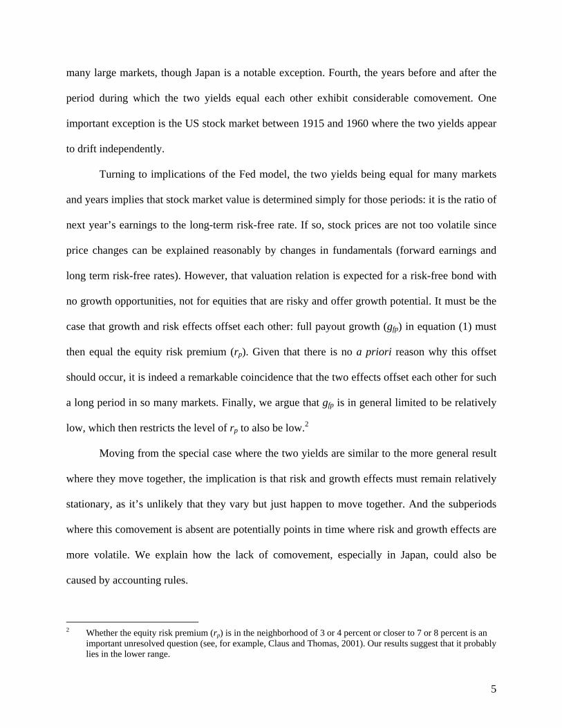
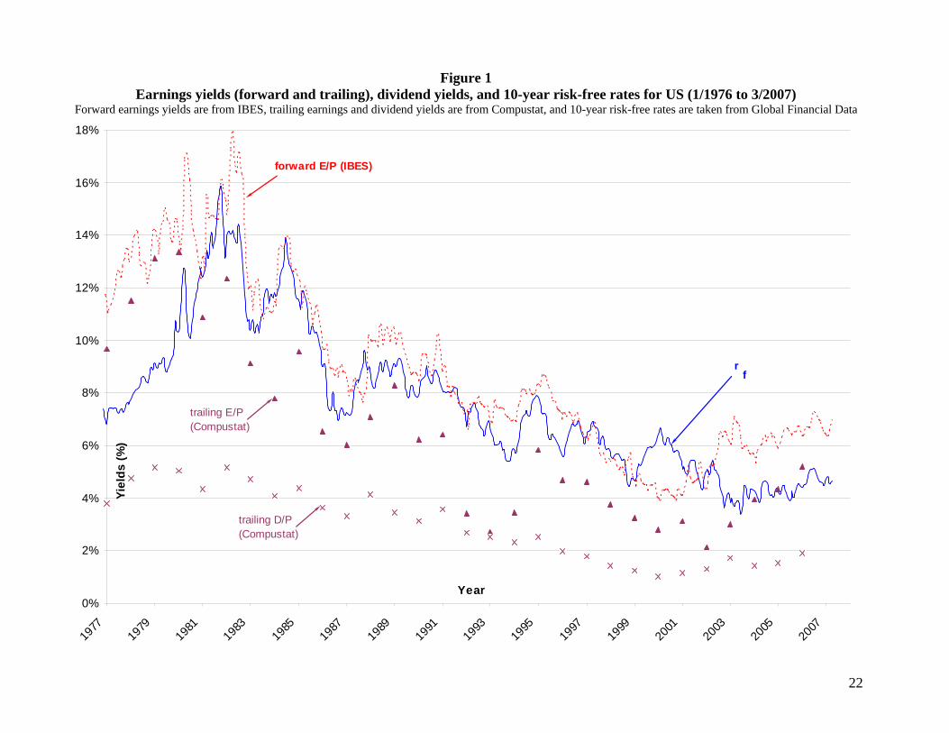
Figure 1 contains the plots for bond yields and forward earnings yields for the US. The

markers on the bottom axis refer to the beginning of each of the years noted; for example, the

data above the 1979 marker corresponds to January, 1979. The main finding is that while the two

series appear to be approximately equal for the period examined in the original Fed report, there

8 If, for example, the month is June 1990, then for a calendar year firm (which would have reported its 1989

earnings some time earlier in 1990), the forecast we use will be for the year 1991. We supplement number of shares outstanding on IBES with data from the CRSP monthly files (for US firms only).

9 For France and Germany, we use the Benchmark 10-year yields as the Government bond series was incomplete. For earlier years for some markets, if the daily data is missing, we substituted the end of the month yields. For the US, prior to April, 1953, we use the yields for Treasury bonds with maturity greater than 10 years.

11

is evidence of the two yields deviating in other subperiods. Specifically, earnings yields exceed

bond yields in the late 1970’s and after 2001, consistent with the equity premium being higher

than the growth term for those years, and there is evidence consistent with the opposite situation

during the late 1990’s.10 More relevant to the question of inflation illusion, the two yields appear

to comove, even during periods when they are not approximately equal to each other.

To supplement these results, we derived forward earnings yields during the 1960’s for a

sample of 174 large US firms described in Cragg and Malkiel (1982). Their data allowed a

calculation of one earnings yield per year, not monthly yields as in Figure 1. While the sample of

firms is relatively small, it consists primarily of large firms and these earnings yields should be

representative of the prevailing aggregate earnings yields. Once again, the results are consistent

with those reported for the 1970’s in Figure 1: forward earnings yields are higher than long–term

rates (about 6 percent vs. about 4 percent), but the two series appear to move together.

Note that analysts’ forecasts for next year (e1) are biased upward, and the 10-year risk-

free rate likely understates the longer-term rate that applies to all future cash flows. While the

extent of bias in forecasted aggregate earnings has not been documented, the median level of

optimism at the firm level is about one percent of price (Table VI in Claus and Thomas, 2001,

for forecasts made between 1985 and 1997).11 And to the extent that 30-year rates are a more

representative estimate of long-term rates than 10-year rates, those rates have exceeded 10-year

rates by about 30 basis points in the US. In effect, adjusting for these two biases suggests that the

10 To be sure, the deviations in the late 1990’s, which coincide with the Internet “bubble”, are also consistent with

stocks being temporarily overpriced in those years. Stated differently, the growth expectations implied by stock prices during those years were unreasonably optimistic.

11 Since the extent of optimism in earnings forecasts declines as the forecasts approach the earnings announcements, and since a majority of US firms have calendar year-ends, forward earnings yields calculated just after annual earnings are announced early in the following year (e.g., in March) will contain more optimism bias than earnings yields calculated just prior to annual earnings announcements (e.g., in January).

12

Fed model can be restated as follows: unbiased estimates of long-term bond yields exceed

unbiased estimates of earnings yields by about 130 basis points.

Readers more familiar with trailing earnings yields or dividend yields may wonder about

the importance of specifying the Fed model in terms of forward earnings yields. To provide

some evidence, we also report in Figure 1 the annual series for trailing earnings yields and

dividend yields (D/P) for all firms with available data on Compustat. Trailing earnings represent

the “bottom line” earnings (including extraordinary items and discontinued operations).

Consider, for example, the markers for trailing earnings and dividends for 1978 which are

reported just to the left of the 1979 tick mark on the horizontal axis. These two markers are based

on earnings and dividends for firm-years ending in December, 1978, as well as all fiscal year-

ends between June, 1978 and May, 1979, and the prices are as of the end of 1978.

While trailing earnings yields lie generally below long-term risk-free rates in Figure 1,

there is clear evidence that trailing yields covary with interest rates. Also, there is a difference of

about 200 basis points between trailing and forward yields, excluding recessions where that gap

increases. There are three reasons why forward yields exceed trailing yields: a) trailing earnings

include write-offs and other charges that are not expected to recur in forward earnings (especially

evident during recessions, such as in the early 1990’s), b) forward earnings for next year include

normal expected growth over the two-year period since the trailing earnings of last year, and

c) analysts’ estimates for forward earnings are optimistic.

Figure 1 also suggests that the Fed model does not apply to trailing dividend yields. Not

only do dividend yields lie far below interest rates, covariation between the two series is harder

to discern, relative to that observed for earnings yields. One reason for this lower level of

covariation is variation over time in dividend payouts: in addition to considerable year to year

13

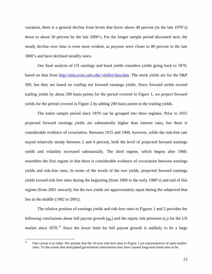
variation, there is a general decline from levels that hover above 40 percent (in the late 1970’s)

down to about 30 percent by the late 2000’s, For the longer sample period discussed next, the

steady decline over time is even more evident, as payouts were closer to 80 percent in the late

1800’s and have declined steadily since.

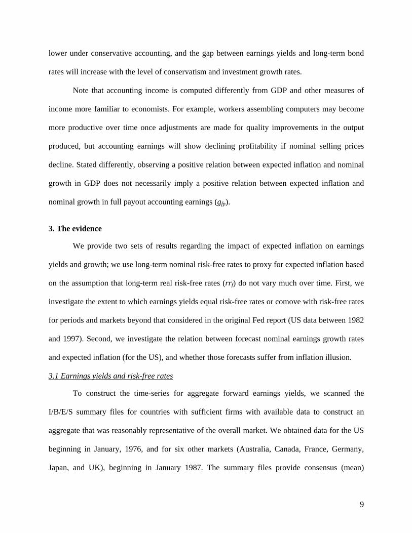
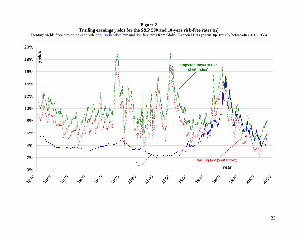
Our final analysis of US earnings and bond yields considers yields going back to 1870,

based on data from http://aida.econ.yale.edu/~shiller/data.htm. The stock yields are for the S&P

500, but they are based on trailing not forward earnings yields. Since forward yields exceed

trailing yields by about 200 basis points for the period covered in Figure 1, we project forward

yields for the period covered in Figure 2 by adding 200 basis points to the trailing yields.

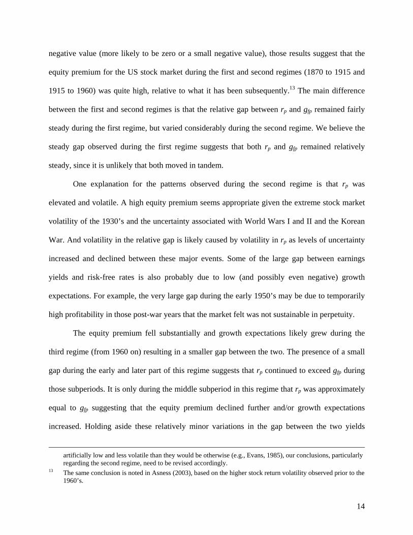
The entire sample period since 1870 can be grouped into three regimes. Prior to 1915

projected forward earnings yields are substantially higher than interest rates, but there is

considerable evidence of covariation. Between 1915 and 1960, however, while the risk-free rate

stayed relatively steady between 2 and 4 percent, both the level of projected forward earnings

yields and volatility increased substantially. The third regime, which begins after 1960,

resembles the first regime in that there is considerable evidence of covariation between earnings

yields and risk-free rates. In terms of the levels of the two yields, projected forward earnings

yields exceed risk-free rates during the beginning (from 1960 to the early 1980’s) and end of this

regime (from 2001 onward), but the two yields are approximately equal during the subperiod that

lies in the middle (1982 to 2001).

The relative position of earnings yields and risk-free rates in Figures 1 and 2 provides the

following conclusions about full payout growth (gfp) and the equity risk premium (rp) for the US

market since 1870.12 Since the lower limit for full payout growth is unlikely to be a large

12 One caveat is in order. We assume that the 10-year risk-free rates in Figure 2 are representative of open market

rates. To the extent that anticipated government intervention may have caused long-term bond rates to be

14

negative value (more likely to be zero or a small negative value), those results suggest that the

equity premium for the US stock market during the first and second regimes (1870 to 1915 and

1915 to 1960) was quite high, relative to what it has been subsequently.13 The main difference

between the first and second regimes is that the relative gap between rp and gfp remained fairly

steady during the first regime, but varied considerably during the second regime. We believe the

steady gap observed during the first regime suggests that both rp and gfp remained relatively

steady, since it is unlikely that both moved in tandem.

One explanation for the patterns observed during the second regime is that rp was

elevated and volatile. A high equity premium seems appropriate given the extreme stock market

volatility of the 1930’s and the uncertainty associated with World Wars I and II and the Korean

War. And volatility in the relative gap is likely caused by volatility in rp as levels of uncertainty

increased and declined between these major events. Some of the large gap between earnings

yields and risk-free rates is also probably due to low (and possibly even negative) growth

expectations. For example, the very large gap during the early 1950’s may be due to temporarily

high profitability in those post-war years that the market felt was not sustainable in perpetuity.

The equity premium fell substantially and growth expectations likely grew during the

third regime (from 1960 on) resulting in a smaller gap between the two. The presence of a small

gap during the early and later part of this regime suggests that rp continued to exceed gfp during

those subperiods. It is only during the middle subperiod in this regime that rp was approximately

equal to gfp suggesting that the equity premium declined further and/or growth expectations

increased. Holding aside these relatively minor variations in the gap between the two yields

artificially low and less volatile than they would be otherwise (e.g., Evans, 1985), our conclusions, particularly regarding the second regime, need to be revised accordingly.

13 The same conclusion is noted in Asness (2003), based on the higher stock return volatility observed prior to the 1960’s.

15

during this third regime, the general pattern of a steady gap for many years in each subperiod

suggests that the equity premium and growth were generally stable over long periods.

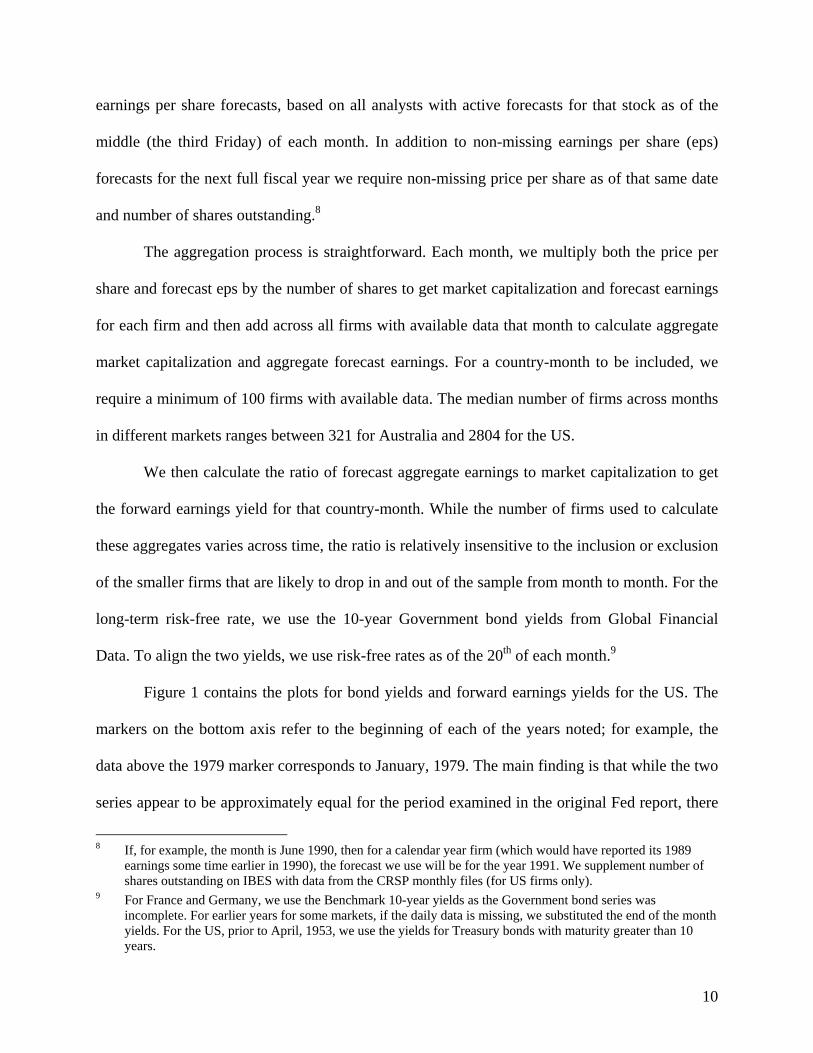
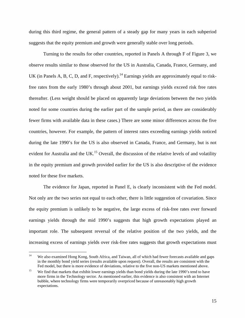
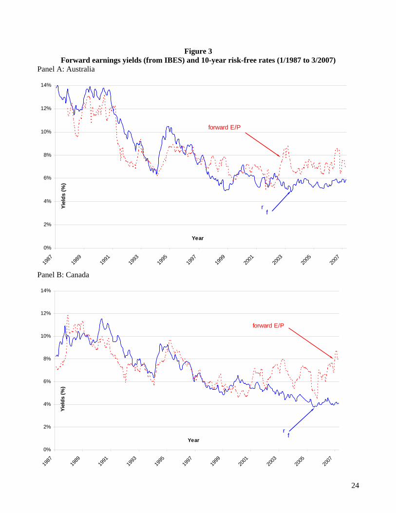
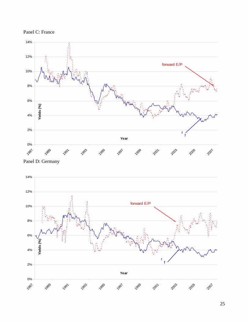
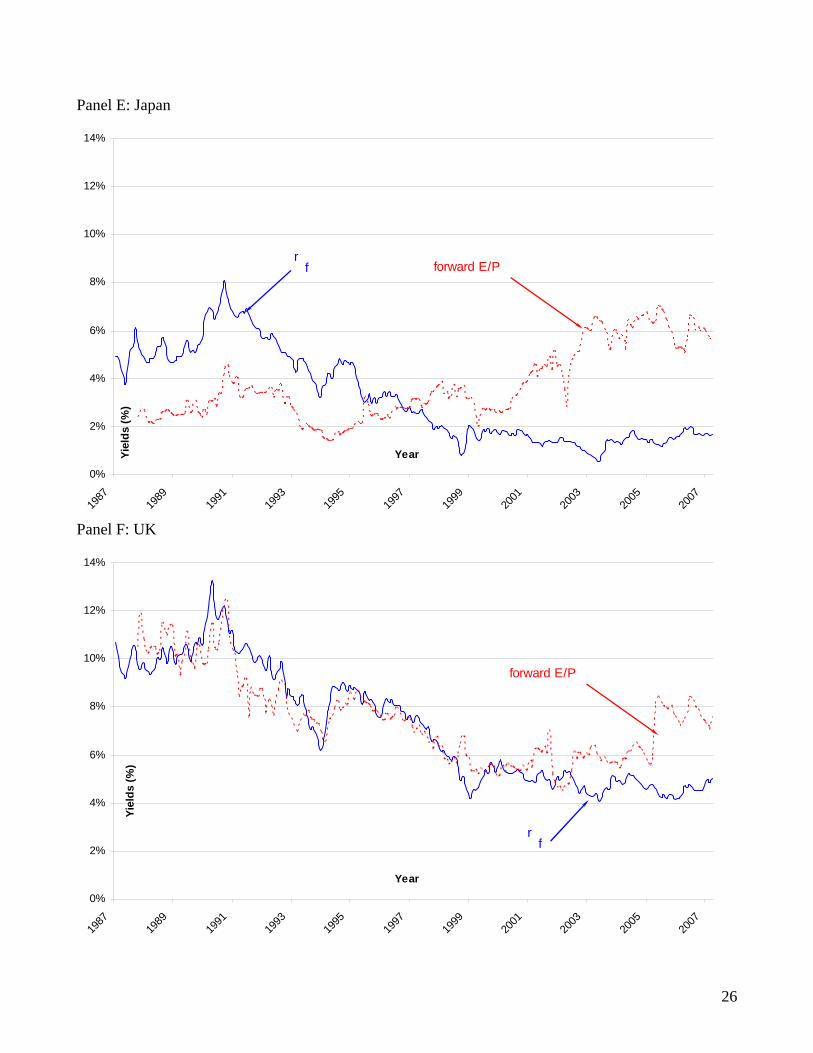
Turning to the results for other countries, reported in Panels A through F of Figure 3, we

observe results similar to those observed for the US in Australia, Canada, France, Germany, and

UK (in Panels A, B, C, D, and F, respectively).14 Earnings yields are approximately equal to risk-

free rates from the early 1980’s through about 2001, but earnings yields exceed risk free rates

thereafter. (Less weight should be placed on apparently large deviations between the two yields

noted for some countries during the earlier part of the sample period, as there are considerably

fewer firms with available data in these cases.) There are some minor differences across the five

countries, however. For example, the pattern of interest rates exceeding earnings yields noticed

during the late 1990’s for the US is also observed in Canada, France, and Germany, but is not

evident for Australia and the UK.15 Overall, the discussion of the relative levels of and volatility

in the equity premium and growth provided earlier for the US is also descriptive of the evidence

noted for these five markets.

The evidence for Japan, reported in Panel E, is clearly inconsistent with the Fed model.

Not only are the two series not equal to each other, there is little suggestion of covariation. Since

the equity premium is unlikely to be negative, the large excess of risk-free rates over forward

earnings yields through the mid 1990’s suggests that high growth expectations played an

important role. The subsequent reversal of the relative position of the two yields, and the

increasing excess of earnings yields over risk-free rates suggests that growth expectations must

14 We also examined Hong Kong, South Africa, and Taiwan, all of which had fewer forecasts available and gaps

in the monthly bond yield series (results available upon request). Overall, the results are consistent with the Fed model, but there is more evidence of deviations, relative to the five non-US markets mentioned above.

15 We find that markets that exhibit lower earnings yields than bond yields during the late 1990’s tend to have more firms in the Technology sector. As mentioned earlier, this evidence is also consistent with an Internet bubble, where technology firms were temporarily overpriced because of unreasonably high growth expectations.

16

be declining substantially. To be sure, an increasing equity premium could also be partially

responsible.

The earlier discussion of accounting rules indicates that deviations from the Fed model

observed in Japan could be due to factors other than growth and risk effects. First, land value

may represent a larger fraction of total asset value for Japanese firms. Historical cost accounting

for land causes earnings yields to be relatively insensitive to expected inflation. Second,

Japanese accounting has traditionally been tied more closely to tax accounting, which results in

more conservative accounting. Since conservatism depresses earnings yields, with the degree of

depression increasing with growth, the lower earnings yields observed before the mid 1990’s

could be driven partially by the combination of conservatism and high growth. Subsequently,

earnings yields may be depressed less as growth expectations declined and the degree of

conservatism also declined as some firms switched from Japanese accounting to International

Accounting Standards. Finally, to the extent that some of the income from Japanese firms is due

to investments in the equity of other firms, each of which represent relatively small percentage

holdings (less than 20%) because of the keiretsu or cross-holding structure that was common in

Japan, the accounting income from those investments is understated because it only includes the

corresponding fraction of dividends paid, not profits earned. To the extent that the fraction of

total income from such holdings has declined in importance, the extent of understatement of

earnings yields would also decline.

3.2 Growth rates and expected inflation

For our second set of results, we return to US analyst data to estimate nominal growth

anticipated by the stock market for the period with I/B/E/S data (since 1977). Whereas financial

economists expect real growth rates to be unrelated to inflation, we show that it is nominal

growth rates that are unrelated to inflation. In fact, analysts’ forecasts of five-year out earnings

17

growth rates remain relatively unchanged over high and low inflation periods. We confirm that

those forecasts of constant growth are not due to inflation illusion by showing that they are

supported by actual growth that is observed subsequently.

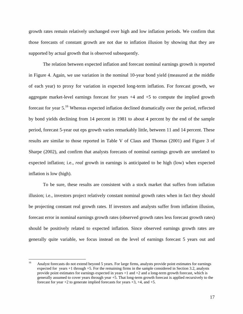
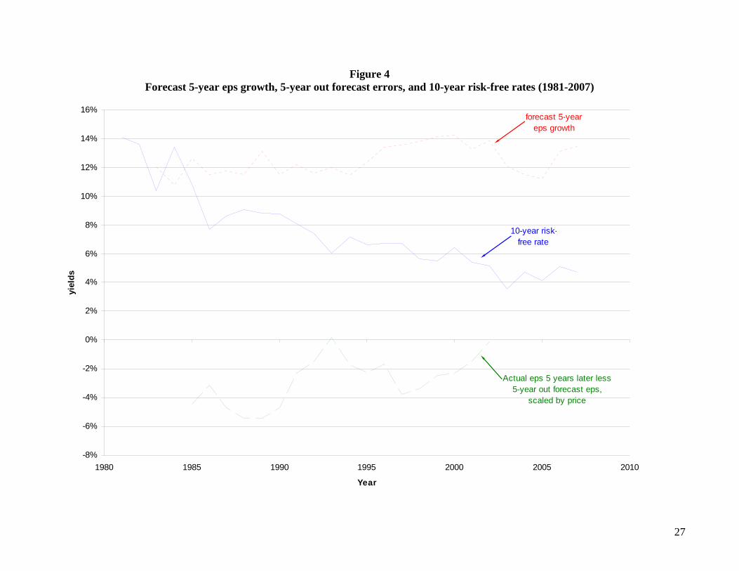
The relation between expected inflation and forecast nominal earnings growth is reported

in Figure 4. Again, we use variation in the nominal 10-year bond yield (measured at the middle

of each year) to proxy for variation in expected long-term inflation. For forecast growth, we

aggregate market-level earnings forecast for years +4 and +5 to compute the implied growth

forecast for year 5.16 Whereas expected inflation declined dramatically over the period, reflected

by bond yields declining from 14 percent in 1981 to about 4 percent by the end of the sample

period, forecast 5-year out eps growth varies remarkably little, between 11 and 14 percent. These

results are similar to those reported in Table V of Claus and Thomas (2001) and Figure 3 of

Sharpe (2002), and confirm that analysts forecasts of nominal earnings growth are unrelated to

expected inflation; i.e., real growth in earnings is anticipated to be high (low) when expected

inflation is low (high).

To be sure, these results are consistent with a stock market that suffers from inflation

illusion; i.e., investors project relatively constant nominal growth rates when in fact they should

be projecting constant real growth rates. If investors and analysts suffer from inflation illusion,

forecast error in nominal earnings growth rates (observed growth rates less forecast growth rates)

should be positively related to expected inflation. Since observed earnings growth rates are

generally quite variable, we focus instead on the level of earnings forecast 5 years out and

16 Analyst forecasts do not extend beyond 5 years. For large firms, analysts provide point estimates for earnings

expected for years +1 through +5. For the remaining firms in the sample considered in Section 3.2, analysts provide point estimates for earnings expected in years +1 and +2 and a long-term growth forecast, which is generally assumed to cover years through year +5. That long-term growth forecast is applied recursively to the forecast for year +2 to generate implied forecasts for years +3, +4, and +5.

18

compare it with the actual earnings reported 5 years later.17 This forecast error is scaled by

current market capitalization.18 If investors should be using a constant real growth rate, forecast

nominal growth rates should be positively related to expected inflation. By projecting constant

nominal growth rates, earnings forecasts should be less optimistic when inflation is high early in

the sample period and should be more optimistic as expected inflation declines over time. That

is, forecast errors should be less negative early in the sample period and then grow increasingly

negative over time.

The bottom line reported in Figure 4 describes variation over time in the 5-year out

forecast error. These forecast errors are generally negative, confirming that analyst forecasts tend

to be optimistic. However, there is no indication that forecasts are becoming increasingly

optimistic over time as expected inflation declined. In fact, the slight upward trend in this line

suggests that optimism may have declined over time. In effect, our results run counter to the

suggestion that real growth rates should be unaffected by changes in inflation and are more

consistent with the negative real effects view; i.e., increases in expected inflation have a negative

impact on real cash flows and valuations (e.g., Fama, 1981, and Lucas, 1996).

While our evidence is consistent with a stock market which rationally forecasts nominal

growth rates to be relatively constant but real growth rates to be lower when inflation is higher,

Campbell and Vuolteenaho (2004) conclude exactly the opposite. Using a VAR model to infer

objective expectations regarding future growth, they find that real expected growth is strongly

positively related to expected inflation; i.e., instead of inflation having negative real effects, it

actually has positive real effects. They also find evidence of stock prices being too low (high) 17 We use here the actual earnings as reported by I/B/E/S, which tends to exclude one-time earnings components.

We repeated the plots using actual earnings as reported (from Compustat) and observed similar results. 18 To ensure that the general increase in market capitalization over the sample period does not attenuate the

scaled forecast error, we repeat the plots using total asset instead of market capitalization as the scaling variable. The results remain similar.

19

when inflation is high (low) consistent with the market suffering from inflation illusion caused

by using growth expectations that are systematically too low (high) at those points. Thomas and

Zhang (2007) reinvestigate their dataset and find that their results are sensitive to the period

employed to estimate their model.19 Specifically, when the post-1960 period is used, the VAR

analysis suggests that rational expectations of real expected dividend or earnings growth are

strongly negatively related to expected inflation and there is no evidence of mispricing that is

consistent with inflation illusion. It seems odd that the pre-1960 period is necessary to document

evidence of inflation illusion, since the Fed model does not hold in those years and no inflation

illusion is expected based on the data from that period.

4. Discussion

If the Fed model describes rational stock markets, stock price movements can generally

be explained by two fundamentals: changes in forward earnings and changes in interest rates. In

contrast, attempts to relate market valuations with dividends, both contemporaneous and paid in

the future, have typically met with little success. A number of prior papers have concluded that

this weak relation between stock prices and fundamentals (level of dividends and expected

returns) is evidence in support of the view that stock prices are too volatile, in the sense that they

deviate often from fundamentals. (see for example Figure 1 from Grossman and Shiller, 1981).

Apparently, moving from observed future dividends to expected earnings changes dramatically

the inferences regarding excess volatility. Moving from the market level to the firm level, there

is now considerable evidence (e.g. Liu and Thomas, 2000) that a substantial fraction of the

variation in stock prices is explained by levels of forecast earnings and long-term interest rates.

19 Thomas and Zhang (2007) also provide additional robustness checks on the Campbell and Vuolteenaho (2004)

dataset, which suggest that results consistent with inflation illusion are sensitive to the choice of inflation measure as well as the choice of dividends or earnings when measuring growth.

20

The equivalence between full payout growth and risk premia implied by the Fed model

offers insights about the level of and variation over time in the equity premium. As indicated by

our discussion of accounting rules (in section 2) we believe that full payout growth aggregate is

relatively low (less than 5 percent). If so, for periods that are described reasonably by the Fed

model, the equity premium will also lie in the same range. While this level of risk premium is

inconsistent with equity premium around seven percent derived from historic stock returns (e.g.,

Ibbotson, 2007), it is consistent with the lower risk premium estimates that have been proposed

recently in the literature (e.g. Claus and Thomas, 2001, and Fama and French, 2002).20 For other

periods where earnings yields are higher than risk-free rates (such as the first regime in the US,

corresponding to the period before 1915), the equity premium was likely much higher than it is

in more recent periods.

Turning to time-variation in the equity premium, the steady gap between the risk and

growth effects implied by the general evidence of covariation between earnings yields and risk-

free rates suggests that both effects are relatively constant through time. We say so because it

seems unlikely that both risk and growth varied in tandem.

The two pieces of evidence documented that are clearly inconsistent with earnings yields

covarying with interest rates are the results for the US between 1915 and 1960 (Figure 2) and the

results for Japan (Figure 3, Panel E). We do not interpret this contradictory evidence as

suggesting that it is unreasonable to expect the two yields to covary. Rather we believe it

suggests that covariation is generally expected, but the conditions necessary for covariation do

not hold for these two subsamples and offer reasons (such as accounting conservatism) to explain

why covariation is not observed in these two cases. 20 As mentioned in Section 3, analysts’ earnings forecasts are biased upward and the 10-year rate is likely to

understate the true long-term risk-free rate, leaving a net bias effect of about 130 basis points. Incorporating this bias drops the equity premium even further.

21

References

Asness, C., 2003, Fight the Fed model: the relationship between future returns and stock and bond market yields, Journal of Portfolio Management, Fall:11–24.

Campbell, John and Yuomo Vuolteenaho. 2004. Inflation illusion and stock prices. American Economics Review Papers and Proceedings, 19–23.

Claus, J. and J.K. Thomas, 2001. Equity premia as low as three percent? Evidence from analysts’ earnings forecasts for domestic and international stock markets, Journal of Finance. 55: (5), 1629–66.

Cragg, J.G. and B. G. Malkiel. 1982. Expectations and the Structure of Share Prices, University of Chicago Press, Chicago.

Evans, P. 1985. Do Large Deficits Produce High Interest Rates? American Economic Review 75: 68-87.

Fama, Eugene. 1981. Stock returns, real activity, inflation, and money. American Economic Review. 71(4):545–65.

Fama, E.E. and K. R. French, 2002. The equity risk premium. Journal of Finance. (57): 637–59.

Gordon, M., 1962, The Investment, Financing, and Valuation of the Corporation, Irwin, Homewood, IL.

Grossman, S.J., and R.J. Shiller, 1981. The determinants of the variability of stock prices. American Economic Review. (71): 222–7

Liu, J. and J.K. Thomas, 2000. Stock returns and accounting earnings, Journal of Accounting Research. 38: 71-101.

Lucas, Robert, Jr. 1996. Nobel lecture: monetary neutrality. Journal of Political Economy, 104(4): 661–82.

Modigliani, F. and R. Cohn, 1979, Inflation, rational valuation, and the market, Financial Analysts’ Journal. March/April: 24–44.

Riiter, J.R. 2002. The Biggest Mistakes We Teach, Journal of Financial Research. 25: 159–168.

Sharpe, S.A. 2002. Reexamining stock valuation and inflation: The implications of analysts' earnings forecasts, The Review of Economics and Statistics. 84: 632–48.

Thomas, J.K. 2007. Accounting rules and the relation between earnings yields and inflation. Working paper, Yale University, School of Management.

Thomas, J. K. and F. Zhang. 2007. Inflation illusion and stock prices: A comment. Working paper, Yale University, School of Management..

22

Figure 1 Earnings yields (forward and trailing), dividend yields, and 10-year risk-free rates for US (1/1976 to 3/2007)

Forward earnings yields are from IBES, trailing earnings and dividend yields are from Compustat, and 10-year risk-free rates are taken from Global Financial Data

0%

2%

4%

6%

8%

10%

12%

14%

16%

18%

1977

1979

1981

1983

1985

1987

1989

1991

1993

1995

1997

1999

2001

2003

2005

2007

Year

Yiel

ds (%

)

forward E/P (IBES)

trailing E/P (Compustat)

trailing D/P (Compustat)

fr

23

Figure 2 Trailing earnings yields for the S&P 500 and 10-year risk-free rates (rf)

Earnings yields from http://aida.econ.yale.edu/~shiller/data.htm and risk-free rates from Global Financial Data (= tcm10p/ tcm10y before/after 3/31/1953)

0%

2%

4%

6%

8%

10%

12%

14%

16%

18%

20%

1870

1880

1890

1900

1910

1920

1930

1940

1950

1960

1970

1980

1990

2000

2010

Year

yiel

ds

trailing E/P (S&P Index)f

r

projected forward E/P (S&P Index)

24

Figure 3 Forward earnings yields (from IBES) and 10-year risk-free rates (1/1987 to 3/2007)

Panel A: Australia

0%

2%

4%

6%

8%

10%

12%

14%

1987

1989

1991

1993

1995

1997

1999

2001

2003

2005

2007

Year

Yiel

ds (%

)

forward E/P

fr

Panel B: Canada

0%

2%

4%

6%

8%

10%

12%

14%

1987

1989

1991

1993

1995

1997

1999

2001

2003

2005

2007

Year

Yiel

ds (%

)

forward E/P

fr

25

Panel C: France

0%

2%

4%

6%

8%

10%

12%

14%

1987

1989

1991

1993

1995

1997

1999

2001

2003

2005

2007

Year

Yiel

ds (%

)

forward E/P

fr

Panel D: Germany

0%

2%

4%

6%

8%

10%

12%

14%

1987

1989

1991

1993

1995

1997

1999

2001

2003

2005

2007

Year

Yiel

ds (%

)

forward E/P

fr

26

Panel E: Japan

0%

2%

4%

6%

8%

10%

12%

14%

1987

1989

1991

1993

1995

1997

1999

2001

2003

2005

2007

YearYiel

ds (%

)

forward E/Pfr

Panel F: UK

0%

2%

4%

6%

8%

10%

12%

14%

1987

1989

1991

1993

1995

1997

1999

2001

2003

2005

2007

Year

Yiel

ds (%

)

forward E/P

fr

27

Figure 4 Forecast 5-year eps growth, 5-year out forecast errors, and 10-year risk-free rates (1981-2007)

-8%

-6%

-4%

-2%

0%

2%

4%

6%

8%

10%

12%

14%

16%

1980 1985 1990 1995 2000 2005 2010

Year

yiel

ds

forecast 5-year eps growth

10-year risk-free rate

Actual eps 5 years later less5-year out forecast eps,

scaled by price