Embed Size (px)
Citation preview

Introduction to Mixed Modelsfor Longitudinal Continuous Data
Don HedekerUniversity of Illinois at Chicago
[email protected]/∼hedeker/ml.html
Chapters 4 and 5 in Hedeker & Gibbons (2006), Longitudinal Data Analysis, Wiley.
Hedeker, D. (2004). An introduction to growth modeling. In D. Kaplan (Ed.),Quantitative Methodology for the Social Sciences. Thousand Oaks CA: Sage.
1
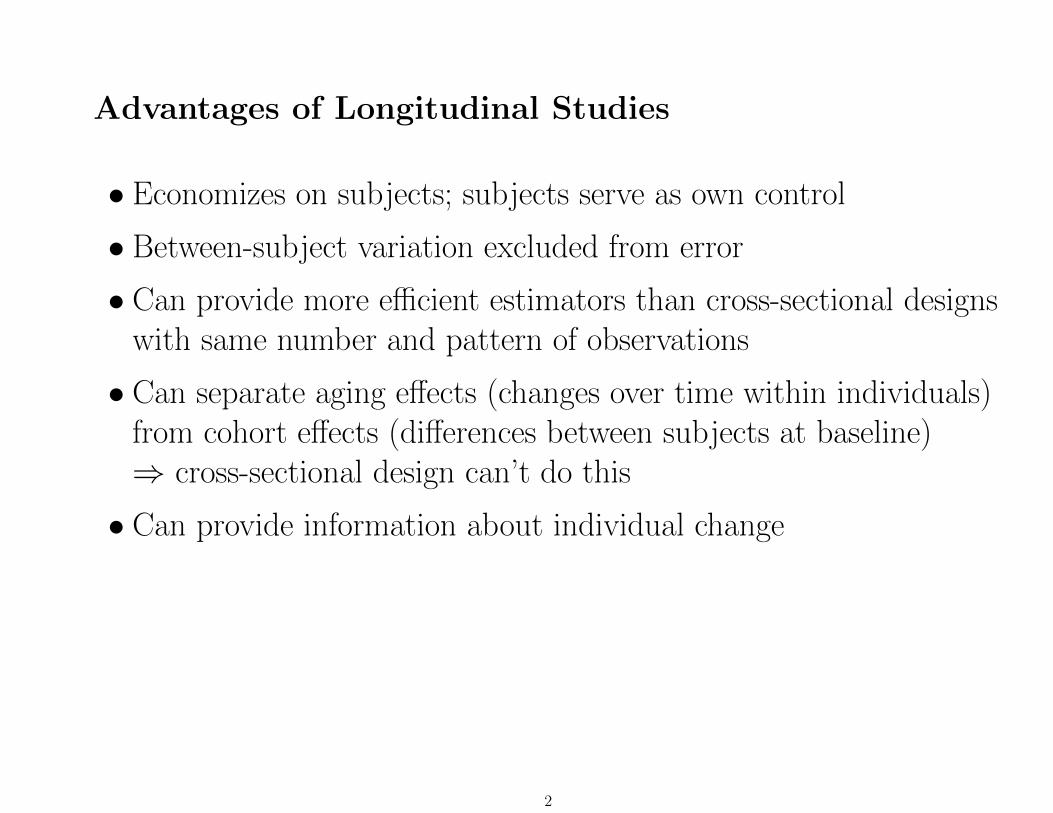
Advantages of Longitudinal Studies
• Economizes on subjects; subjects serve as own control
• Between-subject variation excluded from error
• Can provide more efficient estimators than cross-sectional designswith same number and pattern of observations
• Can separate aging effects (changes over time within individuals)from cohort effects (differences between subjects at baseline)⇒ cross-sectional design can’t do this
• Can provide information about individual change
2
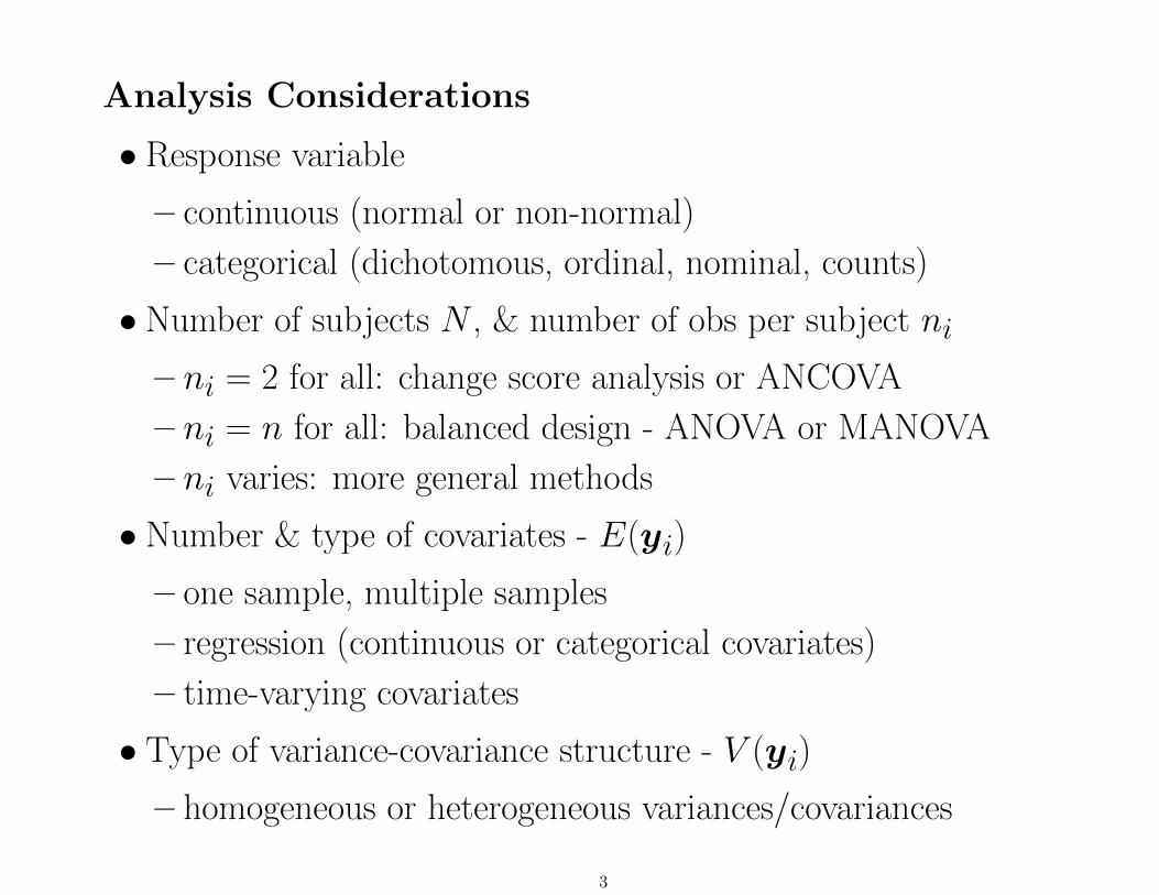
Analysis Considerations
• Response variable
– continuous (normal or non-normal)
– categorical (dichotomous, ordinal, nominal, counts)
• Number of subjects N , & number of obs per subject ni
– ni = 2 for all: change score analysis or ANCOVA
– ni = n for all: balanced design - ANOVA or MANOVA
– ni varies: more general methods
• Number & type of covariates - E(yi)
– one sample, multiple samples
– regression (continuous or categorical covariates)
– time-varying covariates
• Type of variance-covariance structure - V (yi)
– homogeneous or heterogeneous variances/covariances
3

General Approaches
• Derived variable: not really longitudinal, per se, reduce therepeated observations into a summary variable
– average across time, change score, linear trend across time, lastobservation
• Longitudinal Analysis
– ANOVA/MANOVA for repeated measures
– Mixed-effects regression models
– Covariance pattern models
– Generalized Estimating Equations (GEE) models
– Structural Equations Models
– Transition Models
4
Advantages of Mixed-effects Regression Models (MRM)
1. MRM explicitly models individual change across time
2. MRM more flexible in terms of repeated measures
(a) need not have same number of obs per subject
(b) time can be continuous, rather than a fixed set of points
3. Flexible specification of the covariance structure among repeatedmeasures ⇒ methods for testing specific determinants of thisstructure
4. MRM can be extended to higher-level models ⇒ repeatedobservations within individuals within clusters
5. Generalizations for non-normal data
5
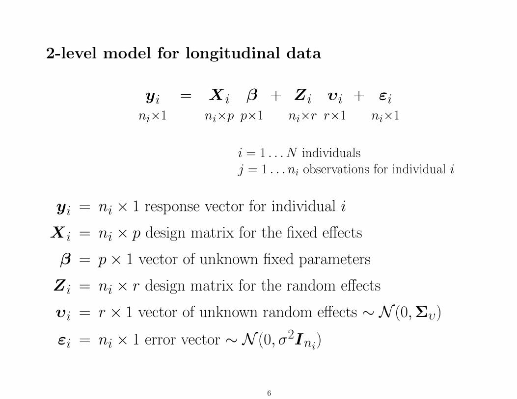
2-level model for longitudinal data
yini×1
= Xini×p
βp×1
+ Zini×r
υir×1
+ εini×1
i = 1 . . . N individualsj = 1 . . . ni observations for individual i
yi = ni × 1 response vector for individual i
Xi = ni × p design matrix for the fixed effects
β = p× 1 vector of unknown fixed parameters
Zi = ni × r design matrix for the random effects
υi = r × 1 vector of unknown random effects ∼ N (0,Συ)
εi = ni × 1 error vector ∼ N (0, σ2Ini)
6
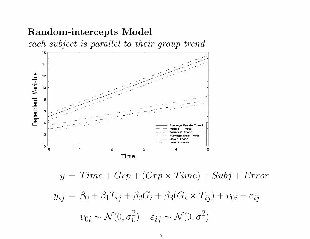
Random-intercepts Modeleach subject is parallel to their group trend
y = Time + Grp + (Grp× Time) + Subj + Error
yij = β0 + β1Tij + β2Gi + β3(Gi × Tij) + υ0i + εij
υ0i ∼ N (0, σ2υ) εij ∼ N (0, σ2)
7
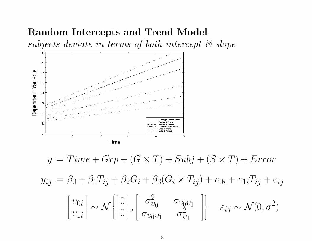
Random Intercepts and Trend Modelsubjects deviate in terms of both intercept & slope
y = Time + Grp + (G× T ) + Subj + (S × T ) + Error
yij = β0 + β1Tij + β2Gi + β3(Gi × Tij) + υ0i + υ1iTij + εijυ0iυ1i
∼ N
00
,σ2υ0
συ0υ1
συ0υ1 σ2υ1
εij ∼ N (0, σ2)
8
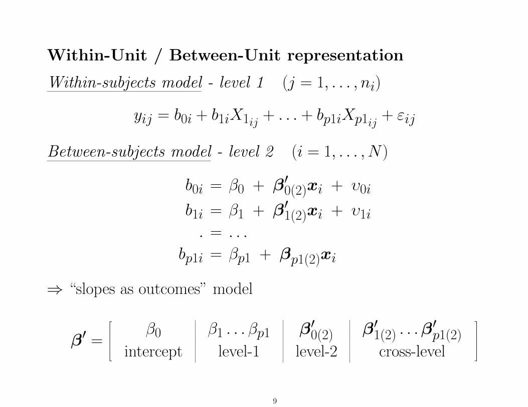
Within-Unit / Between-Unit representation
Within-subjects model - level 1 (j = 1, . . . , ni)
yij = b0i + b1iX1ij + . . . + bp1iXp1ij + εij
Between-subjects model - level 2 (i = 1, . . . , N)
b0i = β0 + β′0(2)xi + υ0i
b1i = β1 + β′1(2)xi + υ1i
. = . . .
bp1i = βp1 + βp1(2)xi
⇒ “slopes as outcomes” model
β′ =
β0 β1 . . . βp1 β′0(2) β′1(2) . . .β
′p1(2)
intercept level-1 level-2 cross-level
9
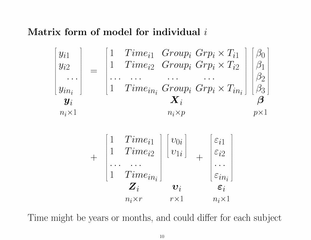
Matrix form of model for individual i
yi1yi2. . .
yini
yini×1
=
1 Timei1 Groupi Grpi × Ti11 Timei2 Groupi Grpi × Ti2. . . . . . . . . . . .1 Timeini Groupi Grpi × Tini
Xini×p
β0β1β2β3
βp×1
+
1 Timei11 Timei2. . . . . .1 Timeini
Zini×r
υ0iυ1i
υir×1
+
εi1εi2. . .εini
εini×1
Time might be years or months, and could differ for each subject
10
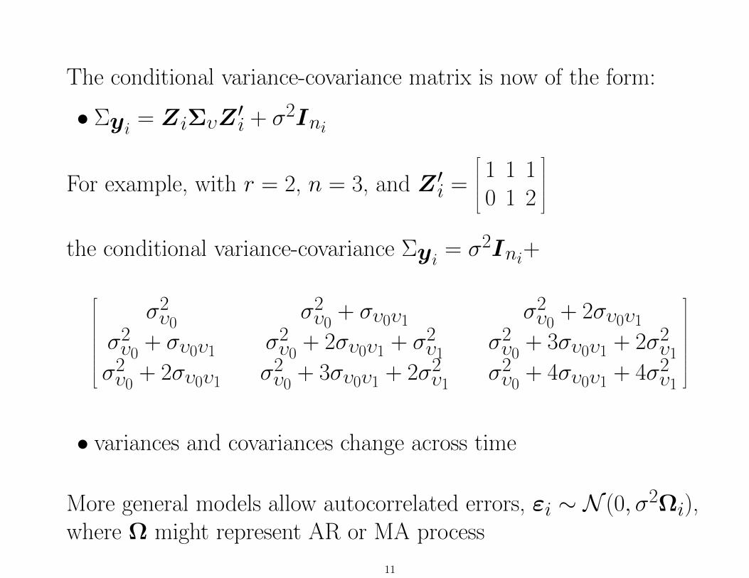
The conditional variance-covariance matrix is now of the form:
• Σyi = ZiΣυZ′i + σ2Ini
For example, with r = 2, n = 3, and Z ′i =
1 1 10 1 2
the conditional variance-covariance Σyi = σ2Ini+
σ2υ0
σ2υ0
+ συ0υ1 σ2υ0
+ 2συ0υ1
σ2υ0
+ συ0υ1 σ2υ0
+ 2συ0υ1 + σ2υ1
σ2υ0
+ 3συ0υ1 + 2σ2υ1
σ2υ0
+ 2συ0υ1 σ2υ0
+ 3συ0υ1 + 2σ2υ1
σ2υ0
+ 4συ0υ1 + 4σ2υ1
• variances and covariances change across time
More general models allow autocorrelated errors, εi ∼ N (0, σ2Ωi),where Ω might represent AR or MA process
11
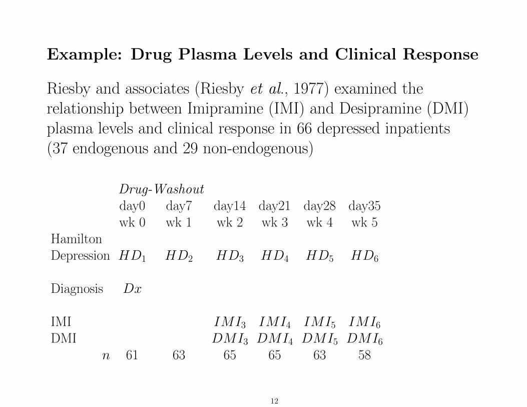
Example: Drug Plasma Levels and Clinical Response
Riesby and associates (Riesby et al., 1977) examined therelationship between Imipramine (IMI) and Desipramine (DMI)plasma levels and clinical response in 66 depressed inpatients(37 endogenous and 29 non-endogenous)
Drug-Washoutday0 day7 day14 day21 day28 day35wk 0 wk 1 wk 2 wk 3 wk 4 wk 5
HamiltonDepression HD1 HD2 HD3 HD4 HD5 HD6
Diagnosis Dx
IMI IMI3 IMI4 IMI5 IMI6
DMI DMI3 DMI4 DMI5 DMI6
n 61 63 65 65 63 58
12
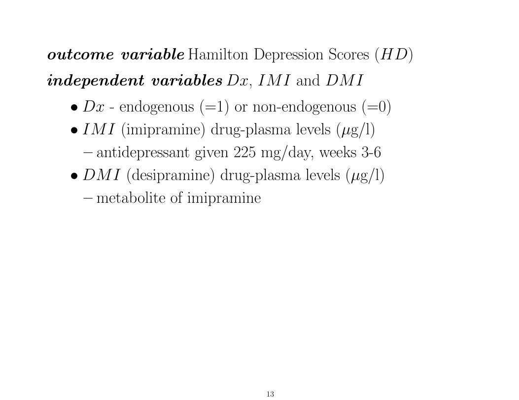
outcome variable Hamilton Depression Scores (HD)
independent variablesDx, IMI and DMI
•Dx - endogenous (=1) or non-endogenous (=0)
• IMI (imipramine) drug-plasma levels (µg/l)
– antidepressant given 225 mg/day, weeks 3-6
•DMI (desipramine) drug-plasma levels (µg/l)
– metabolite of imipramine
13
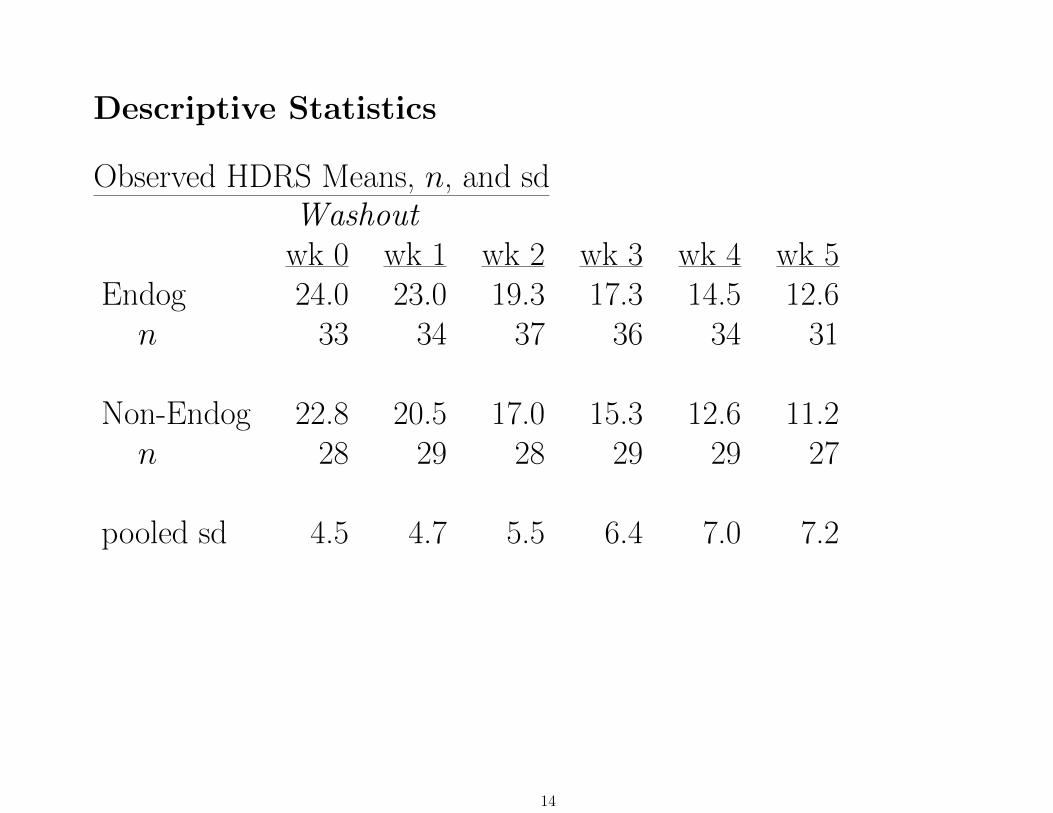
Descriptive Statistics
Observed HDRS Means, n, and sdWashout
wk 0 wk 1 wk 2 wk 3 wk 4 wk 5Endog 24.0 23.0 19.3 17.3 14.5 12.6n 33 34 37 36 34 31
Non-Endog 22.8 20.5 17.0 15.3 12.6 11.2n 28 29 28 29 29 27
pooled sd 4.5 4.7 5.5 6.4 7.0 7.2
14

Correlations: n = 46 and 46 ≤ n ≤ 66
wk 0 wk 1 wk 2 wk 3 wk 4 wk 5week 0 1.0 .49 .41 .33 .23 .18week 1 .49 1.0 .49 .41 .31 .22week 2 .42 .49 1.0 .74 .67 .46week 3 .44 .51 .73 1.0 .82 .57week 4 .30 .35 .68 .78 1.0 .65week 5 .22 .23 .53 .62 .72 1.0
15
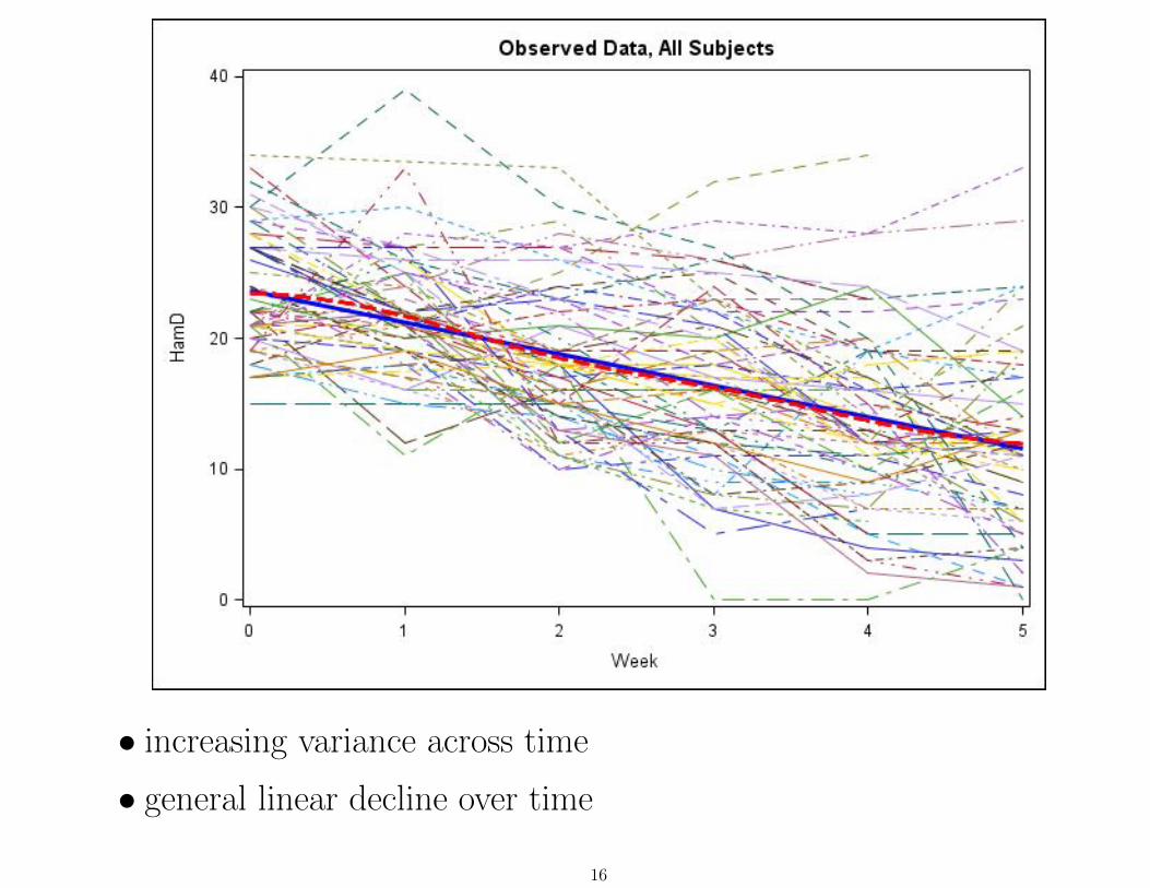
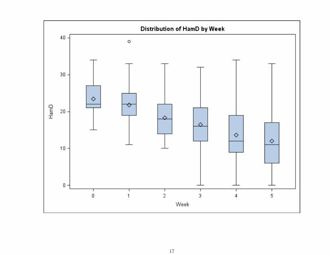
• increasing variance across time
• general linear decline over time
16
17

18
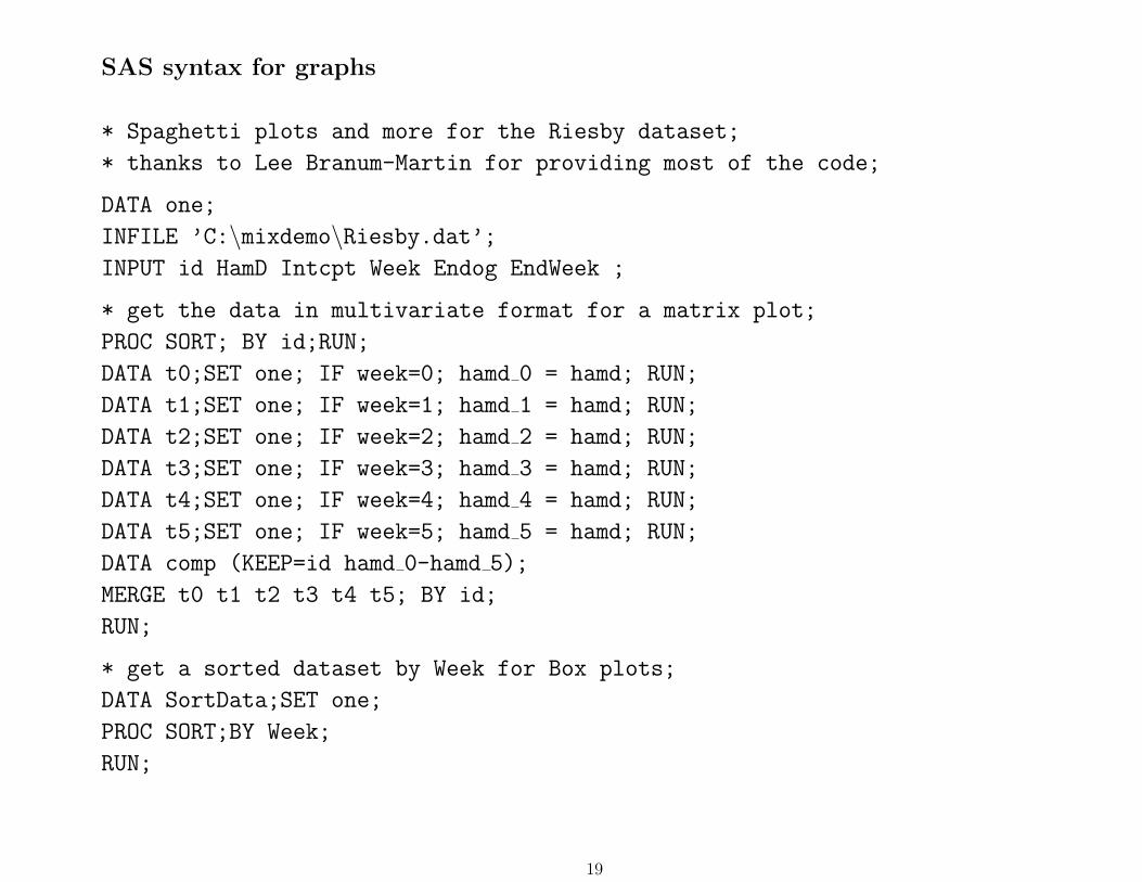
SAS syntax for graphs
* Spaghetti plots and more for the Riesby dataset;
* thanks to Lee Branum-Martin for providing most of the code;
DATA one;
INFILE ’C:\mixdemo\Riesby.dat’;INPUT id HamD Intcpt Week Endog EndWeek ;
* get the data in multivariate format for a matrix plot;
PROC SORT; BY id;RUN;
DATA t0;SET one; IF week=0; hamd 0 = hamd; RUN;
DATA t1;SET one; IF week=1; hamd 1 = hamd; RUN;
DATA t2;SET one; IF week=2; hamd 2 = hamd; RUN;
DATA t3;SET one; IF week=3; hamd 3 = hamd; RUN;
DATA t4;SET one; IF week=4; hamd 4 = hamd; RUN;
DATA t5;SET one; IF week=5; hamd 5 = hamd; RUN;
DATA comp (KEEP=id hamd 0-hamd 5);
MERGE t0 t1 t2 t3 t4 t5; BY id;
RUN;
* get a sorted dataset by Week for Box plots;
DATA SortData;SET one;
PROC SORT;BY Week;
RUN;
19
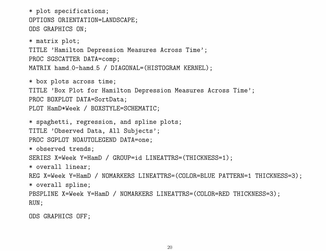
* plot specifications;
OPTIONS ORIENTATION=LANDSCAPE;
ODS GRAPHICS ON;
* matrix plot;
TITLE ’Hamilton Depression Measures Across Time’;
PROC SGSCATTER DATA=comp;
MATRIX hamd 0-hamd 5 / DIAGONAL=(HISTOGRAM KERNEL);
* box plots across time;
TITLE ’Box Plot for Hamilton Depression Measures Across Time’;
PROC BOXPLOT DATA=SortData;
PLOT HamD*Week / BOXSTYLE=SCHEMATIC;
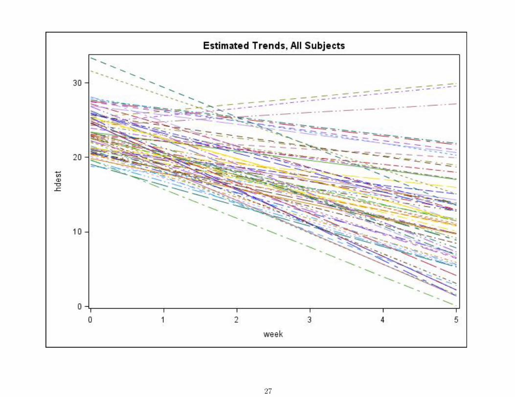
* spaghetti, regression, and spline plots;
TITLE ’Observed Data, All Subjects’;
PROC SGPLOT NOAUTOLEGEND DATA=one;
* observed trends;
SERIES X=Week Y=HamD / GROUP=id LINEATTRS=(THICKNESS=1);
* overall linear;
REG X=Week Y=HamD / NOMARKERS LINEATTRS=(COLOR=BLUE PATTERN=1 THICKNESS=3);
* overall spline;
PBSPLINE X=Week Y=HamD / NOMARKERS LINEATTRS=(COLOR=RED THICKNESS=3);
RUN;
ODS GRAPHICS OFF;
20
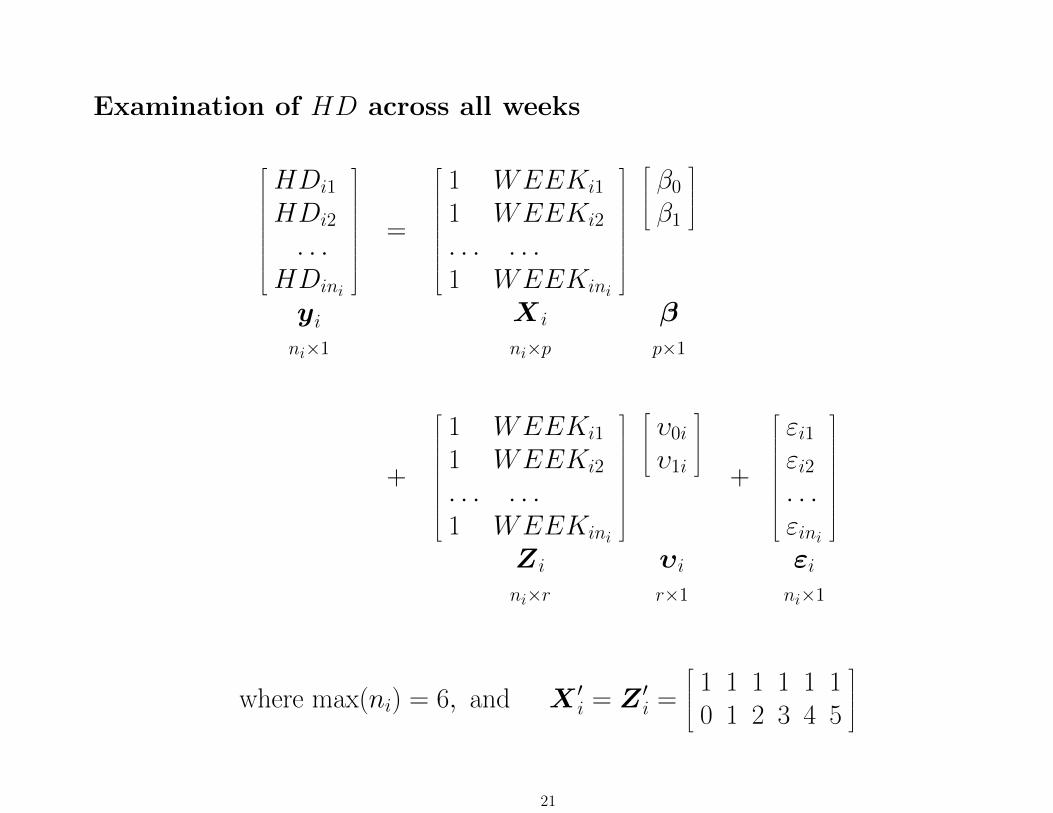
Examination of HD across all weeks
HDi1
HDi2
. . .HDini
yini×1
=
1 WEEKi1
1 WEEKi2
. . . . . .1 WEEKini
X i
ni×p
β0
β1
βp×1
+
1 WEEKi1
1 WEEKi2
. . . . . .1 WEEKini
Z i
ni×r
υ0i
υ1i
υir×1
+
εi1εi2. . .εini
εini×1
where max(ni) = 6, and X ′i = Z ′i =
1 1 1 1 1 10 1 2 3 4 5
21
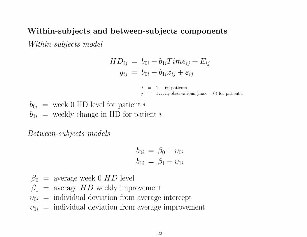
Within-subjects and between-subjects components
Within-subjects model
HDij = b0i + b1iTimeij + Eij
yij = b0i + b1ixij + εij
i = 1 . . . 66 patientsj = 1 . . . ni observations (max = 6) for patient i
b0i = week 0 HD level for patient ib1i = weekly change in HD for patient i
Between-subjects models
b0i = β0 + υ0i
b1i = β1 + υ1i
β0 = average week 0 HD levelβ1 = average HD weekly improvementυ0i = individual deviation from average interceptυ1i = individual deviation from average improvement
22

parameter ML estimate se z p <
β0 23.58 0.55 43.22 .0001β1 -2.38 0.21 -11.39 .0001
σ2υ0
12.63 3.47συ0υ1 -1.42 1.03σ2υ1
2.08 0.50
σ2 12.22 1.11
logL = −1109.52
χ22 = 66.1, p < .0001 for H0 : συ0υ1 = σ2
υ1= 0
συ0υ1 as corr between intercept and slope = -0.28
•Wald tests are dubious for variance parameters, likelihood-ratio tests arepreferred (though divide p-value by 2)
•Wald z-statistics sometimes expressed as χ21 (by squaring z-value)
23
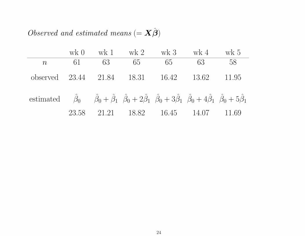
Observed and estimated means (= Xβ)
wk 0 wk 1 wk 2 wk 3 wk 4 wk 5n 61 63 65 65 63 58
observed 23.44 21.84 18.31 16.42 13.62 11.95
estimated β0 β0 + β1 β0 + 2β1 β0 + 3β1 β0 + 4β1 β0 + 5β1
23.58 21.21 18.82 16.45 14.07 11.69
24

Obs. (pairwise) and est. variance-covariance matrix
Σy =
20.55
10.50 22.07
10.20 12.74 30.09
9.69 12.43 25.96 41.15
7.17 10.10 25.56 36.54 48.59
6.02 7.39 18.25 26.31 32.93 52.12
Σy = ZΣυZ′ + σ2I
=
24.85
11.21 24.08
9.79 12.52 27.48
8.37 13.18 18.00 35.03
6.95 13.84 20.73 27.63 46.74
5.53 14.50 23.47 32.44 41.41 62.60
Z ′ =
1 1 1 1 1 1
0 1 2 3 4 5
Συ =
12.63 −1.42
−1.42 2.08
note: from random-int model: σ2υ = 16.16 and σ2 = 19.04
25

26
27

Software for Mixed Models
SAS
• Singer, J. D. (1998). Using SAS PROC MIXED To Fit Multilevel Models, Hierarchical Models, andIndividual Growth Models. Journal of Educational and Behavioral Statistics, 23, 323-355.
• Singer, J. D. (2002). Fitting individual growth models using SAS PROC MIXED. In D. S. Moskowitz &S. L. Hershberger (Eds.), Modeling intraindividual variability with repeated measures data: Methods andapplications (pp. 135-170). Mahwah, NJ: Erlbaum.
• Littell, R.C., Milliken, G.A., Stroup, W.W., Wolfinger, R.D. & Schabenberger, O. (2006). SAS for MixedModels, 2nd edition. Cary NC: SAS Institute.
SPSS
• Peugh, J. L. and Enders, C. K. (2005). Using the SPSS Mixed Procedure to Fit Cross-Sectional andLongitudinal Multilevel Models. Educational and Psychological Measurement, 65, 717-741.
• Painter, J. Notes on using SPSS Mixed Models.http://www.unc.edu/∼painter/SPSSMixed/SPSSMixedModels.PDF
• Heck, R.H., Thomas, S.L., & Tabata, L.N. (2010). Multilevel and Longitudinal Modeling with IBM SPSS.New York: Routledge.
Stata
• Rabe-Hesketh, S. & Skrondal, A. (2012). Multilevel and Longitudinal Modeling using Stata, 3rd edition.College Station, TX: Stata Press.
28
SuperMix
• Free student and 15-day trial editionshttp://www.ssicentral.com/supermix/downloads.html
• Datasets and exampleshttp://www.ssicentral.com/supermix/examples.html
•Manual and documentation in PDF formhttp://www.ssicentral.com/supermix/resources.html
also HLM, MLwiN, lme4 in R, ...
29
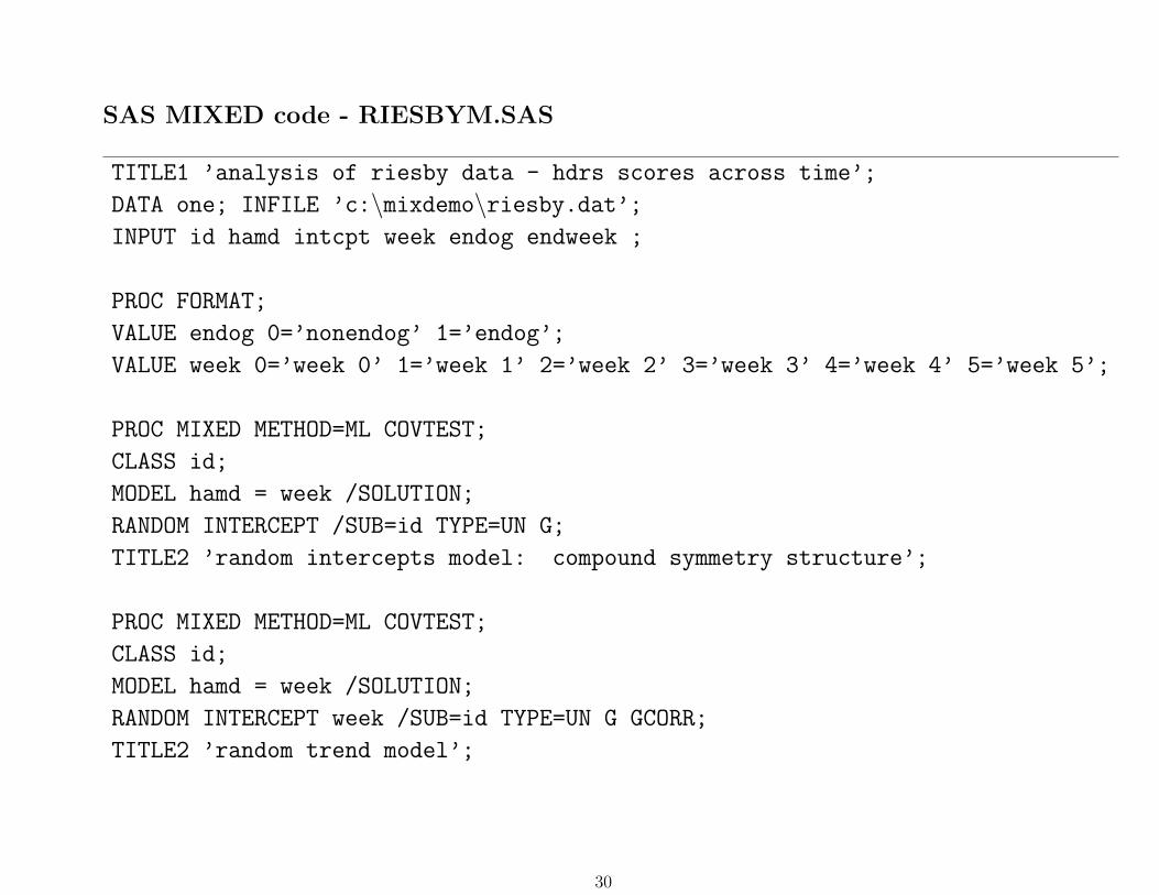
SAS MIXED code - RIESBYM.SAS
TITLE1 ’analysis of riesby data - hdrs scores across time’;
DATA one; INFILE ’c:\mixdemo\riesby.dat’;INPUT id hamd intcpt week endog endweek ;
PROC FORMAT;
VALUE endog 0=’nonendog’ 1=’endog’;
VALUE week 0=’week 0’ 1=’week 1’ 2=’week 2’ 3=’week 3’ 4=’week 4’ 5=’week 5’;
PROC MIXED METHOD=ML COVTEST;
CLASS id;
MODEL hamd = week /SOLUTION;
RANDOM INTERCEPT /SUB=id TYPE=UN G;
TITLE2 ’random intercepts model: compound symmetry structure’;
PROC MIXED METHOD=ML COVTEST;
CLASS id;
MODEL hamd = week /SOLUTION;
RANDOM INTERCEPT week /SUB=id TYPE=UN G GCORR;
TITLE2 ’random trend model’;
30
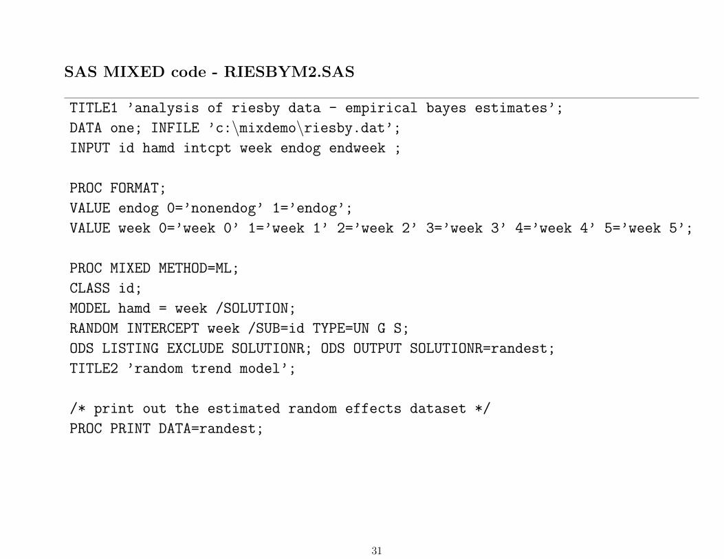
SAS MIXED code - RIESBYM2.SAS
TITLE1 ’analysis of riesby data - empirical bayes estimates’;
DATA one; INFILE ’c:\mixdemo\riesby.dat’;INPUT id hamd intcpt week endog endweek ;
PROC FORMAT;
VALUE endog 0=’nonendog’ 1=’endog’;
VALUE week 0=’week 0’ 1=’week 1’ 2=’week 2’ 3=’week 3’ 4=’week 4’ 5=’week 5’;
PROC MIXED METHOD=ML;
CLASS id;
MODEL hamd = week /SOLUTION;
RANDOM INTERCEPT week /SUB=id TYPE=UN G S;
ODS LISTING EXCLUDE SOLUTIONR; ODS OUTPUT SOLUTIONR=randest;
TITLE2 ’random trend model’;
/* print out the estimated random effects dataset */
PROC PRINT DATA=randest;
31
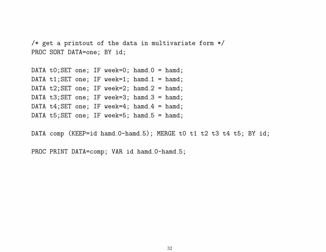
/* get a printout of the data in multivariate form */
PROC SORT DATA=one; BY id;
DATA t0;SET one; IF week=0; hamd 0 = hamd;
DATA t1;SET one; IF week=1; hamd 1 = hamd;
DATA t2;SET one; IF week=2; hamd 2 = hamd;
DATA t3;SET one; IF week=3; hamd 3 = hamd;
DATA t4;SET one; IF week=4; hamd 4 = hamd;
DATA t5;SET one; IF week=5; hamd 5 = hamd;
DATA comp (KEEP=id hamd 0-hamd 5); MERGE t0 t1 t2 t3 t4 t5; BY id;
PROC PRINT DATA=comp; VAR id hamd 0-hamd 5;
32
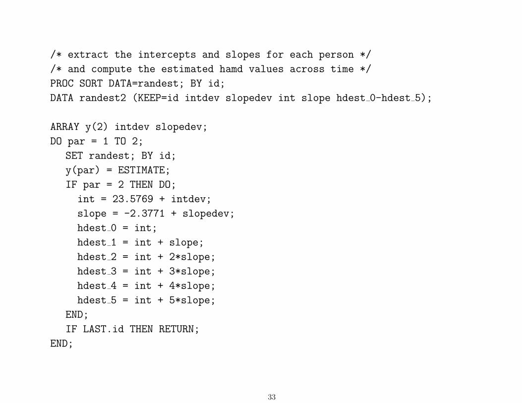
/* extract the intercepts and slopes for each person */
/* and compute the estimated hamd values across time */
PROC SORT DATA=randest; BY id;
DATA randest2 (KEEP=id intdev slopedev int slope hdest 0-hdest 5);
ARRAY y(2) intdev slopedev;
DO par = 1 TO 2;
SET randest; BY id;
y(par) = ESTIMATE;
IF par = 2 THEN DO;
int = 23.5769 + intdev;
slope = -2.3771 + slopedev;
hdest 0 = int;
hdest 1 = int + slope;
hdest 2 = int + 2*slope;
hdest 3 = int + 3*slope;
hdest 4 = int + 4*slope;
hdest 5 = int + 5*slope;
END;
IF LAST.id THEN RETURN;
END;
33

PROC PRINT DATA=randest2; VAR id hdest 0-hdest 5;
PROC PLOT DATA=randest2;
PLOT intdev * slopedev;
PLOT int * slope;
TITLE2 ’plot of individual intercepts versus slopes’;
RUN;
34
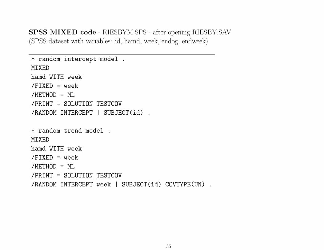
SPSS MIXED code - RIESBYM.SPS - after opening RIESBY.SAV
(SPSS dataset with variables: id, hamd, week, endog, endweek)
* random intercept model .
MIXED
hamd WITH week
/FIXED = week
/METHOD = ML
/PRINT = SOLUTION TESTCOV
/RANDOM INTERCEPT | SUBJECT(id) .
* random trend model .
MIXED
hamd WITH week
/FIXED = week
/METHOD = ML
/PRINT = SOLUTION TESTCOV
/RANDOM INTERCEPT week | SUBJECT(id) COVTYPE(UN) .
35
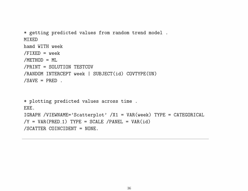
* getting predicted values from random trend model .
MIXED
hamd WITH week
/FIXED = week
/METHOD = ML
/PRINT = SOLUTION TESTCOV
/RANDOM INTERCEPT week | SUBJECT(id) COVTYPE(UN)
/SAVE = PRED .
* plotting predicted values across time .
EXE.
IGRAPH /VIEWNAME=’Scatterplot’ /X1 = VAR(week) TYPE = CATEGORICAL
/Y = VAR(PRED 1) TYPE = SCALE /PANEL = VAR(id)
/SCATTER COINCIDENT = NONE.
36
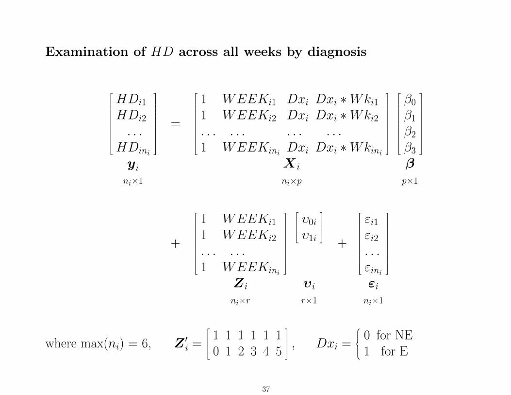
Examination of HD across all weeks by diagnosis
HDi1
HDi2
. . .HDini
yini×1
=
1 WEEKi1 Dxi Dxi ∗Wki11 WEEKi2 Dxi Dxi ∗Wki2. . . . . . . . . . . .1 WEEKini Dxi Dxi ∗Wkini
X i
ni×p
β0
β1
β2
β3
βp×1
+
1 WEEKi1
1 WEEKi2
. . . . . .1 WEEKini
Z i
ni×r
υ0i
υ1i
υir×1
+
εi1εi2. . .εini
εini×1
where max(ni) = 6, Z ′i =
1 1 1 1 1 10 1 2 3 4 5
, Dxi =
0 for NE1 for E
37

Within-subjects and between-subjects components
Within-subjects model
HDij = b0i + b1iTimeij + Eij
b0i = week 0 HD level for patient ib1i = weekly change in HD for patient i
Between-subjects models
b0i = β0 + β2Dxi + υ0i
b1i = β1 + β3Dxi + υ1i
β0 = average week 0 HD level for NE patients (Dxi = 0)β1 = average HD weekly improvement for NE patients (Dxi = 0)β2 = average week 0 HD difference for E patientsβ3 = average HD weekly improvement difference for endogenous patientsυ0i = individual deviation from average interceptυ1i = individual deviation from average improvement
38
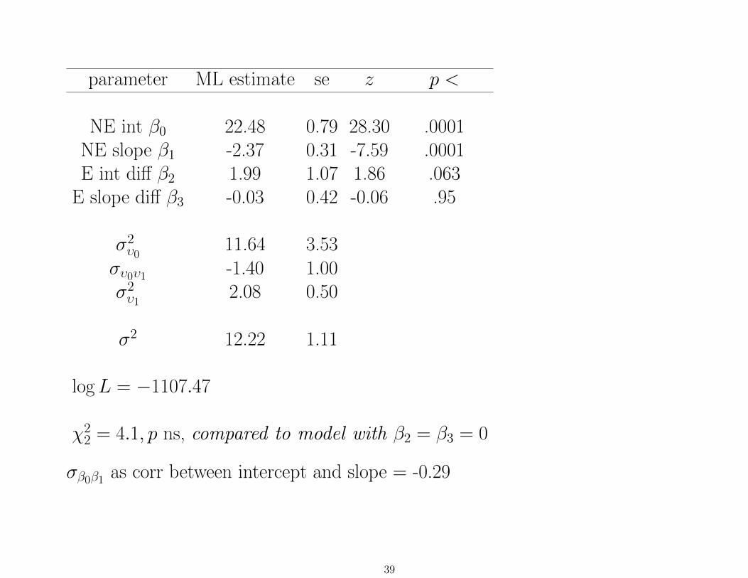
parameter ML estimate se z p <
NE int β0 22.48 0.79 28.30 .0001NE slope β1 -2.37 0.31 -7.59 .0001E int diff β2 1.99 1.07 1.86 .063
E slope diff β3 -0.03 0.42 -0.06 .95
σ2υ0
11.64 3.53συ0υ1 -1.40 1.00σ2υ1
2.08 0.50
σ2 12.22 1.11
logL = −1107.47
χ22 = 4.1, p ns, compared to model with β2 = β3 = 0
σβ0β1 as corr between intercept and slope = -0.29
39
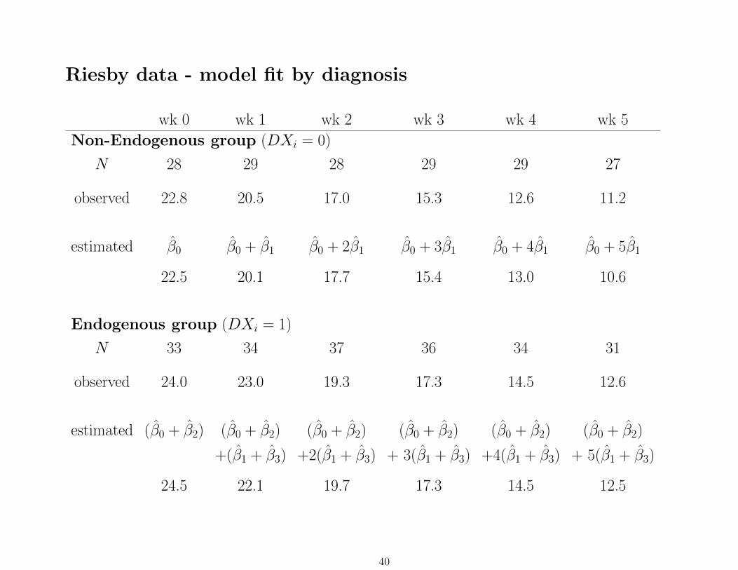
Riesby data - model fit by diagnosis
wk 0 wk 1 wk 2 wk 3 wk 4 wk 5
Non-Endogenous group (DXi = 0)
N 28 29 28 29 29 27
observed 22.8 20.5 17.0 15.3 12.6 11.2
estimated β0 β0 + β1 β0 + 2β1 β0 + 3β1 β0 + 4β1 β0 + 5β1
22.5 20.1 17.7 15.4 13.0 10.6
Endogenous group (DXi = 1)
N 33 34 37 36 34 31
observed 24.0 23.0 19.3 17.3 14.5 12.6
estimated (β0 + β2) (β0 + β2) (β0 + β2) (β0 + β2) (β0 + β2) (β0 + β2)
+(β1 + β3) +2(β1 + β3) + 3(β1 + β3) +4(β1 + β3) + 5(β1 + β3)
24.5 22.1 19.7 17.3 14.5 12.5
40
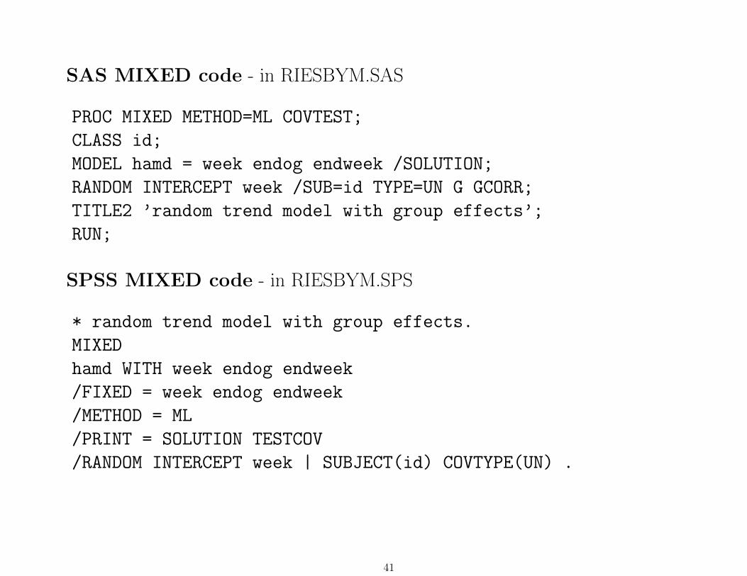
SAS MIXED code - in RIESBYM.SAS
PROC MIXED METHOD=ML COVTEST;
CLASS id;
MODEL hamd = week endog endweek /SOLUTION;
RANDOM INTERCEPT week /SUB=id TYPE=UN G GCORR;
TITLE2 ’random trend model with group effects’;
RUN;
SPSS MIXED code - in RIESBYM.SPS
* random trend model with group effects.
MIXED
hamd WITH week endog endweek
/FIXED = week endog endweek
/METHOD = ML
/PRINT = SOLUTION TESTCOV
/RANDOM INTERCEPT week | SUBJECT(id) COVTYPE(UN) .
41
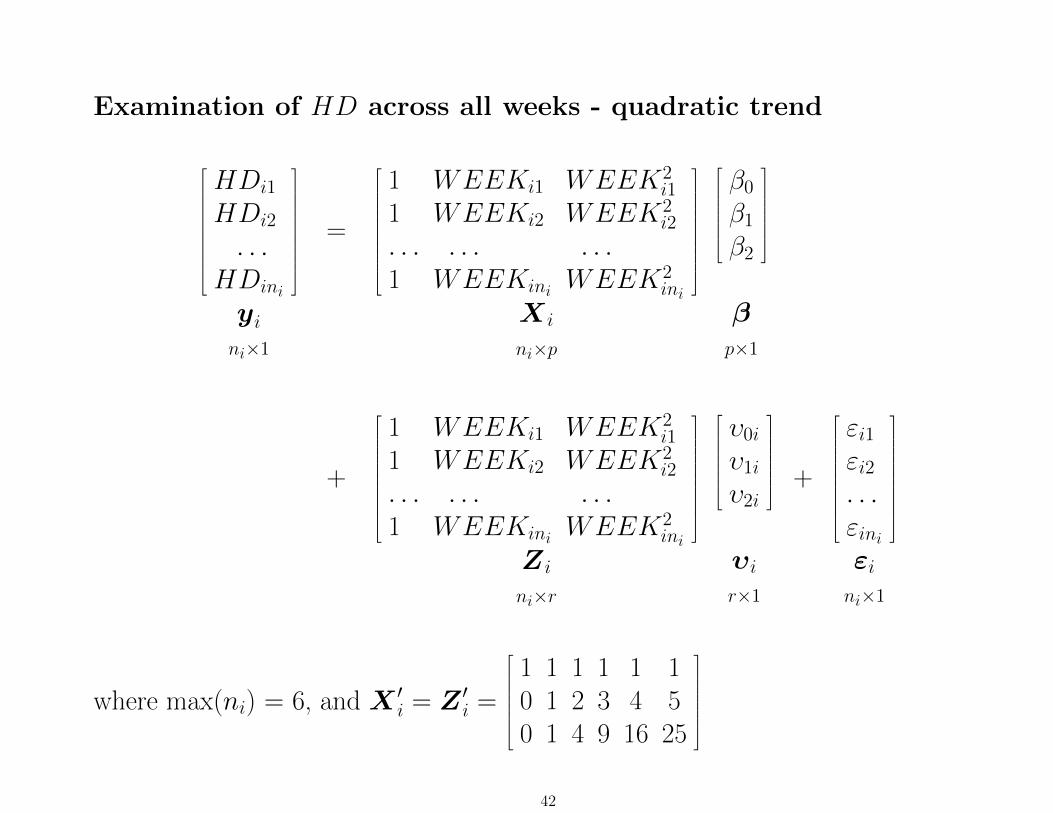
Examination of HD across all weeks - quadratic trend
HDi1
HDi2
. . .HDini
yini×1
=
1 WEEKi1 WEEK2i1
1 WEEKi2 WEEK2i2
. . . . . . . . .1 WEEKini WEEK2
ini
X i
ni×p
β0
β1
β2
βp×1
+
1 WEEKi1 WEEK2i1
1 WEEKi2 WEEK2i2
. . . . . . . . .1 WEEKini WEEK2
ini
Z i
ni×r
υ0i
υ1i
υ2i
υir×1
+
εi1εi2. . .εini
εini×1
where max(ni) = 6, and X ′i = Z ′i =
1 1 1 1 1 10 1 2 3 4 50 1 4 9 16 25
42

Within-subjects and between-subjects componentsWithin-subjects model
HDij = b0i + b1iTimeij + b2iTime2ij + Eij
yij = b0i + b1ixij + b2ix2ij + εij
b0i = week 0 HD level for patient ib1i = weekly linear change in HD for patient ib2i = weekly quadratic change in HD for patient i
Between-subjects modelsb0i = β0 + υ0i
b1i = β1 + υ1i
b2i = β2 + υ2i
β0 = average week 0 HD levelβ1 = average HD weekly linear changeβ2 = average HD weekly quadratic changeυ0i = individual deviation from average interceptυ1i = individual deviation from average linear changeυ2i = individual deviation from average quadratic change
43
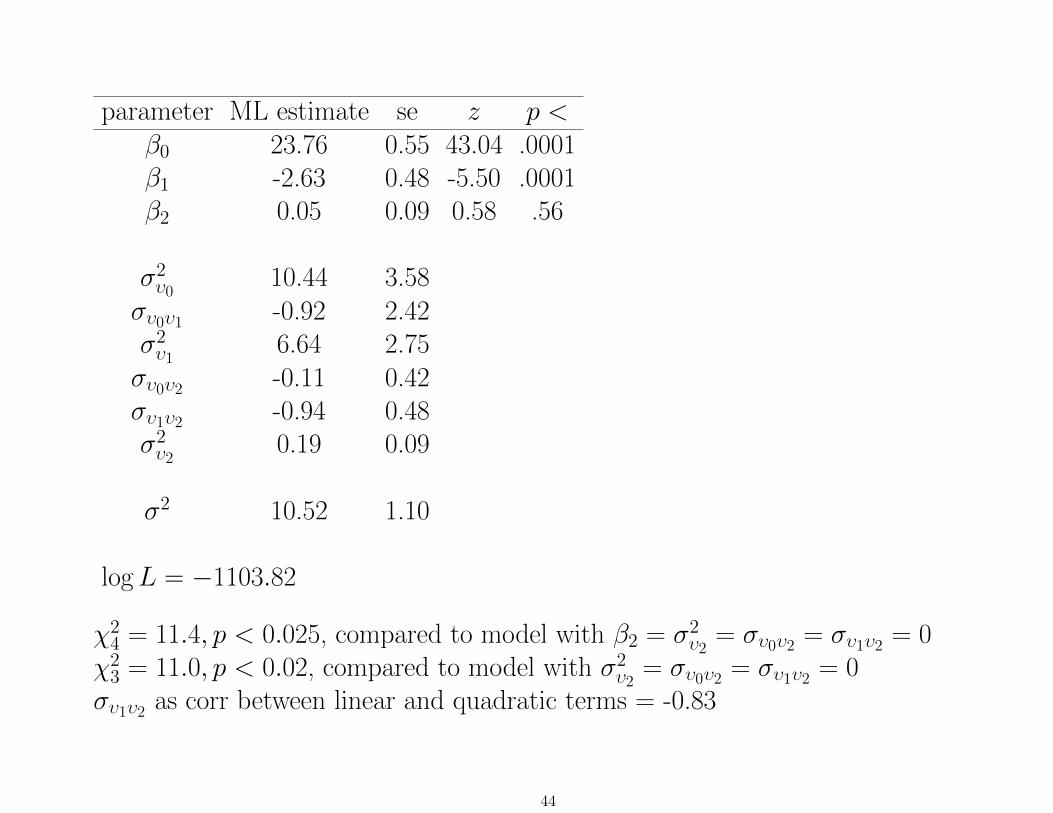
parameter ML estimate se z p <β0 23.76 0.55 43.04 .0001β1 -2.63 0.48 -5.50 .0001β2 0.05 0.09 0.58 .56
σ2υ0
10.44 3.58συ0υ1 -0.92 2.42σ2υ1
6.64 2.75συ0υ2 -0.11 0.42συ1υ2 -0.94 0.48σ2υ2
0.19 0.09
σ2 10.52 1.10
logL = −1103.82
χ24 = 11.4, p < 0.025, compared to model with β2 = σ2
υ2= συ0υ2 = συ1υ2 = 0
χ23 = 11.0, p < 0.02, compared to model with σ2
υ2= συ0υ2 = συ1υ2 = 0
συ1υ2 as corr between linear and quadratic terms = -0.83
44
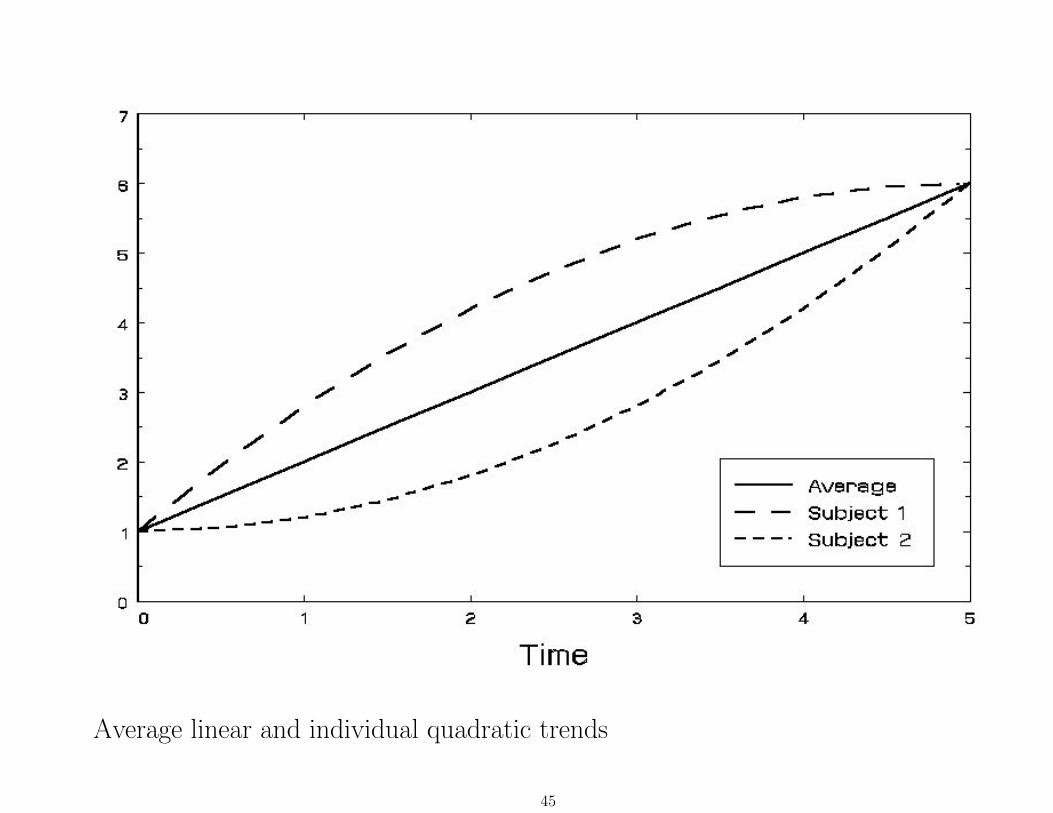
Average linear and individual quadratic trends
45
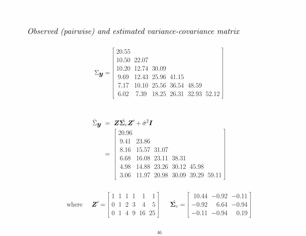
Observed (pairwise) and estimated variance-covariance matrix
Σy =
20.55
10.50 22.07
10.20 12.74 30.09
9.69 12.43 25.96 41.15
7.17 10.10 25.56 36.54 48.59
6.02 7.39 18.25 26.31 32.93 52.12
Σy = ZΣυZ′ + σ2I
=
20.96
9.41 23.86
8.16 15.57 31.07
6.68 16.08 23.11 38.31
4.98 14.88 23.26 30.12 45.98
3.06 11.97 20.98 30.09 39.29 59.11
where Z ′ =
1 1 1 1 1 1
0 1 2 3 4 5
0 1 4 9 16 25
Συ =
10.44 −0.92 −0.11
−0.92 6.64 −0.94
−0.11 −0.94 0.19
46

SAS MIXED code in RIESBYM.SAS
PROC MIXED METHOD=ML COVTEST;
CLASS id;
MODEL hamd = week week*week /SOLUTION;
RANDOM INTERCEPT week week*week /SUB=id TYPE=UN G GCORR;
TITLE2 ’random quadratic trend model’;
RUN;
SPSS MIXED code in RIESBYM.SPS
* compute time squared .
COMPUTE week2 = week*week .
EXECUTE .
* random quadratic trend model .
MIXED
hamd WITH week week2
/FIXED = week week2
/METHOD = ML
/PRINT = SOLUTION TESTCOV
/RANDOM INTERCEPT week week2 | SUBJECT(id) COVTYPE(UN) .
47
Time-varying Covariates - WS and BS effects
Section 4.5.2 in Hedeker & Gibbons (2006), Longitudinal DataAnalysis, Wiley.
48
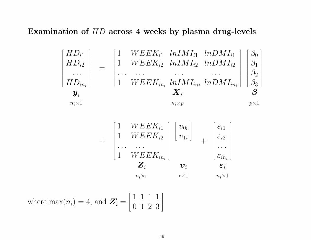
Examination of HD across 4 weeks by plasma drug-levels
HDi1
HDi2
. . .HDini
yini×1
=
1 WEEKi1 lnIMIi1 lnDMIi11 WEEKi2 lnIMIi2 lnDMIi2. . . . . . . . . . . .1 WEEKini lnIMIini lnDMIini
X i
ni×p
β0
β1
β2
β3
βp×1
+
1 WEEKi1
1 WEEKi2
. . . . . .1 WEEKini
Z i
ni×r
υ0i
υ1i
υir×1
+
εi1εi2. . .εini
εini×1
where max(ni) = 4, and Z ′i =
1 1 1 10 1 2 3
49

Within-subjects and between-subjects components
Within-subjects model
HDij = b0i + b1iTij + b2i ln IMIij + b3i lnDMIij + Resij
b0i = week 2 HD level for patient i with both ln IMI and lnDMI = 0b1i = weekly change in HD for patient ib2i = change in HD due to ln IMIb3i = change in HD due to lnDMI
Between-subjects models
b0i = β0 + υ0i
b1i = β1 + υ1i
b2i = β2
b3i = β3
50

β0 = average week 2 HD level for drug-free patientsβ1 = average HD weekly improvementβ2 = average HD difference for unit change in ln IMIβ3 = average HD difference for unit change in lnDMIυ0i = individual intercept deviation from modelυ1i = individual slope deviation from model
Here, week 2 is the actual study week (i.e., one week after the drug washoutperiod), which is coded as 0 in this analysis of the last four study timepoints
51
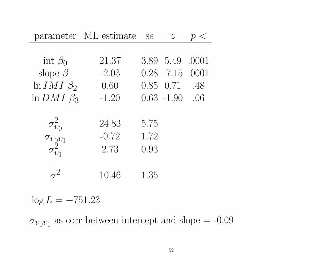
parameter ML estimate se z p <
int β0 21.37 3.89 5.49 .0001slope β1 -2.03 0.28 -7.15 .0001
ln IMI β2 0.60 0.85 0.71 .48lnDMI β3 -1.20 0.63 -1.90 .06
σ2υ0
24.83 5.75
συ0υ1 -0.72 1.72
σ2υ1
2.73 0.93
σ2 10.46 1.35
logL = −751.23
συ0υ1 as corr between intercept and slope = -0.09
52
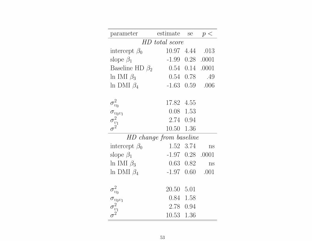
parameter estimate se p <
HD total score
intercept β0 10.97 4.44 .013
slope β1 -1.99 0.28 .0001
Baseline HD β2 0.54 0.14 .0001
ln IMI β3 0.54 0.78 .49
ln DMI β4 -1.63 0.59 .006
σ2υ0
17.82 4.55
συ0υ1 0.08 1.53
σ2υ1
2.74 0.94
σ2 10.50 1.36
HD change from baseline
intercept β0 1.52 3.74 ns
slope β1 -1.97 0.28 .0001
ln IMI β3 0.63 0.82 ns
ln DMI β4 -1.97 0.60 .001
σ2υ0
20.50 5.01
συ0υ1 0.84 1.58
σ2υ1
2.78 0.94
σ2 10.53 1.36
53
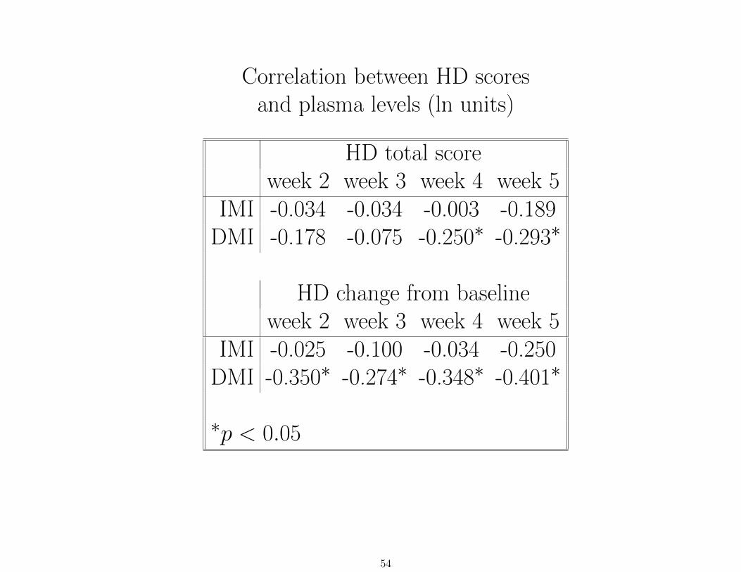
Correlation between HD scoresand plasma levels (ln units)
HD total scoreweek 2 week 3 week 4 week 5
IMI -0.034 -0.034 -0.003 -0.189DMI -0.178 -0.075 -0.250∗ -0.293∗
HD change from baselineweek 2 week 3 week 4 week 5
IMI -0.025 -0.100 -0.034 -0.250DMI -0.350∗ -0.274∗ -0.348∗ -0.401∗
∗p < 0.05
54
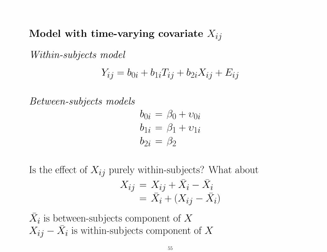
Model with time-varying covariate Xij
Within-subjects model
Yij = b0i + b1iTij + b2iXij + Eij
Between-subjects modelsb0i = β0 + υ0i
b1i = β1 + υ1i
b2i = β2
Is the effect of Xij purely within-subjects? What about
Xij = Xij + Xi − Xi= Xi + (Xij − Xi)
Xi is between-subjects component of XXij − Xi is within-subjects component of X
55
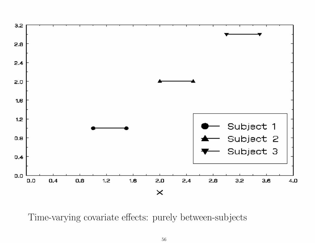
Time-varying covariate effects: purely between-subjects
56
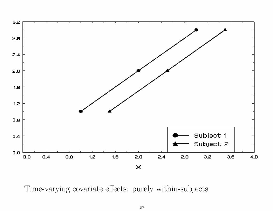
Time-varying covariate effects: purely within-subjects
57
Model with decomposition of time-varying covariate Xij
Within-subjects model
Yij = b0i + b1iTij + b2i(Xij − Xi) + Eij
Between-subjects models
b0i = β0 + βBSXi + υ0i
b1i = β1 + υ1i
b2i = βWS
Notice, effect of X is now βBSXi + βWS(Xij − Xi)
βBS = effect of Xi on Yi BS or “cross-sectional”
βWS = effect of (Xij − Xi) on (Yij − Yi) WS or “longitudinal”
58
Model with only Xij assumes equal BS and WS effects(βBS = βWS)
suppose βBS = βWS = β∗, then in the model with decomposition,
the effect of Xij = β∗Xi + β∗(Xij − Xi) = β∗Xij
⇒ precisely what the model with only Xij assumes
Equal WS and BS effects of Xij?
• can be a dubious assumption
• needs to be tested (by comparing two models via LR test)
• there is no guarantee that βBS and βWS even agree on sign
59

Time-varying covariate effects: opposite sign WS and BS effects
60
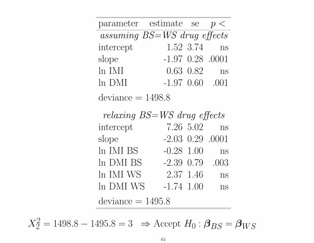
parameter estimate se p <assuming BS=WS drug effectsintercept 1.52 3.74 nsslope -1.97 0.28 .0001ln IMI 0.63 0.82 nsln DMI -1.97 0.60 .001
deviance = 1498.8
relaxing BS=WS drug effectsintercept 7.26 5.02 nsslope -2.03 0.29 .0001ln IMI BS -0.28 1.00 nsln DMI BS -2.39 0.79 .003ln IMI WS 2.37 1.46 nsln DMI WS -1.74 1.00 ns
deviance = 1495.8
X22 = 1498.8− 1495.8 = 3 ⇒ Accept H0 : βBS = βWS
61
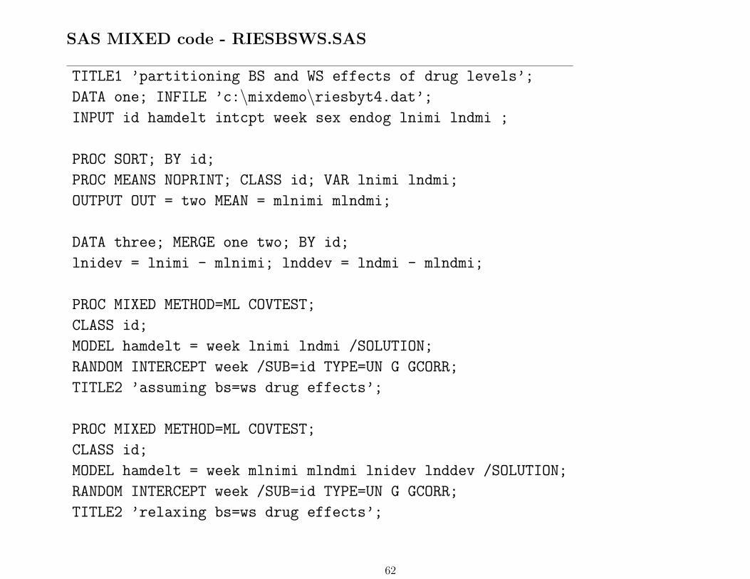
SAS MIXED code - RIESBSWS.SAS
TITLE1 ’partitioning BS and WS effects of drug levels’;
DATA one; INFILE ’c:\mixdemo\riesbyt4.dat’;INPUT id hamdelt intcpt week sex endog lnimi lndmi ;
PROC SORT; BY id;
PROC MEANS NOPRINT; CLASS id; VAR lnimi lndmi;
OUTPUT OUT = two MEAN = mlnimi mlndmi;
DATA three; MERGE one two; BY id;
lnidev = lnimi - mlnimi; lnddev = lndmi - mlndmi;
PROC MIXED METHOD=ML COVTEST;
CLASS id;
MODEL hamdelt = week lnimi lndmi /SOLUTION;
RANDOM INTERCEPT week /SUB=id TYPE=UN G GCORR;
TITLE2 ’assuming bs=ws drug effects’;
PROC MIXED METHOD=ML COVTEST;
CLASS id;
MODEL hamdelt = week mlnimi mlndmi lnidev lnddev /SOLUTION;
RANDOM INTERCEPT week /SUB=id TYPE=UN G GCORR;
TITLE2 ’relaxing bs=ws drug effects’;
62
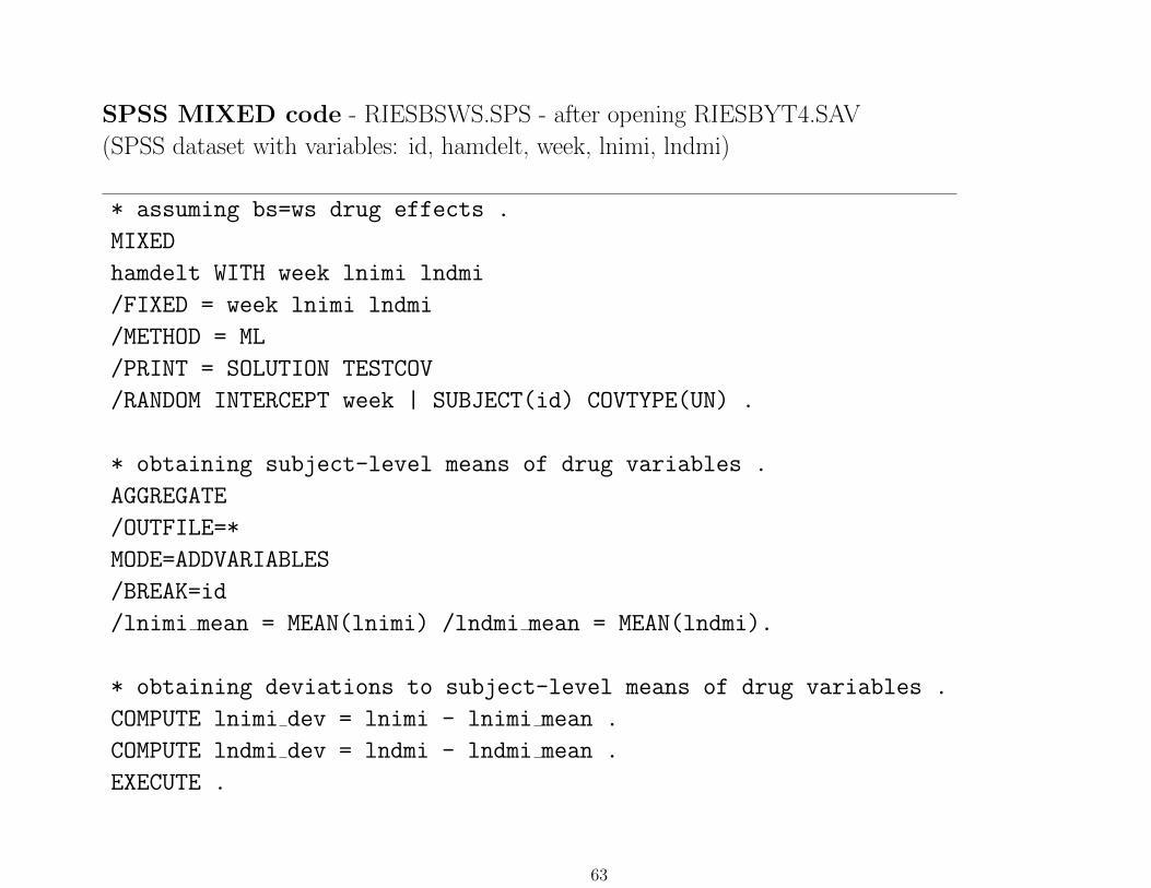
SPSS MIXED code - RIESBSWS.SPS - after opening RIESBYT4.SAV
(SPSS dataset with variables: id, hamdelt, week, lnimi, lndmi)
* assuming bs=ws drug effects .
MIXED
hamdelt WITH week lnimi lndmi
/FIXED = week lnimi lndmi
/METHOD = ML
/PRINT = SOLUTION TESTCOV
/RANDOM INTERCEPT week | SUBJECT(id) COVTYPE(UN) .
* obtaining subject-level means of drug variables .
AGGREGATE
/OUTFILE=*
MODE=ADDVARIABLES
/BREAK=id
/lnimi mean = MEAN(lnimi) /lndmi mean = MEAN(lndmi).
* obtaining deviations to subject-level means of drug variables .
COMPUTE lnimi dev = lnimi - lnimi mean .
COMPUTE lndmi dev = lndmi - lndmi mean .
EXECUTE .
63
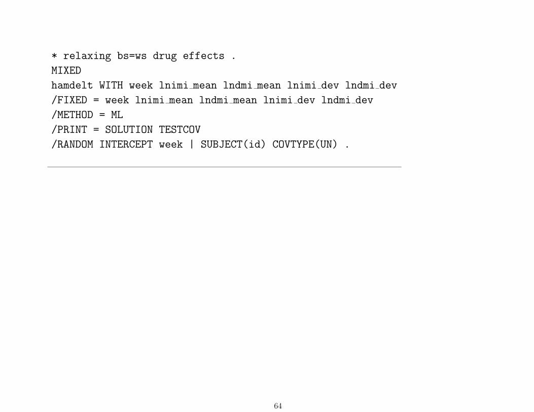
* relaxing bs=ws drug effects .
MIXED
hamdelt WITH week lnimi mean lndmi mean lnimi dev lndmi dev
/FIXED = week lnimi mean lndmi mean lnimi dev lndmi dev
/METHOD = ML
/PRINT = SOLUTION TESTCOV
/RANDOM INTERCEPT week | SUBJECT(id) COVTYPE(UN) .
64