Domokos Peter´ April 19, 2016

Lecture notes on laser spectroscopy and laser cooling

Domokos Peter

April 19, 2016

Contents

1 Review of quantum electrodynamics 11.1 The coupled system of electromagnetic fields and charges . . . . . . . . . 1

1.1.1 The Lorentz-Maxwell equations . . . . . . . . . . . . . . . . . . . 11.1.2 The Maxwell equations in reciprocal space . . . . . . . . . . . . . 21.1.3 Vector and scalar potentials . . . . . . . . . . . . . . . . . . . . . . 4

1.2 The Lagrangian of electrodynamics in the Coulomb gauge . . . . . . . . 61.2.1 Gauge transformations of the Lagrangian . . . . . . . . . . . . . . 8

1.3 The minimal coupling Hamiltonian . . . . . . . . . . . . . . . . . . . . . . 91.4 QED with normal variables . . . . . . . . . . . . . . . . . . . . . . . . . . 10

1.4.1 Discretization of the space . . . . . . . . . . . . . . . . . . . . . . . 11

2 Atom model and dipole interaction with the field 132.1 Dipole approximation . . . . . . . . . . . . . . . . . . . . . . . . . . . . . 13

2.1.1 Unitary transformation into the length gauge . . . . . . . . . . . . 142.1.2 The dipole Hamiltonian . . . . . . . . . . . . . . . . . . . . . . . . 16

2.2 Two-level atom . . . . . . . . . . . . . . . . . . . . . . . . . . . . . . . . . 172.2.1 Pauli spin operators . . . . . . . . . . . . . . . . . . . . . . . . . . 18

3 Spontaneous emission 203.1 Free field and source term in normal order . . . . . . . . . . . . . . . . . 213.2 Markov-approximation . . . . . . . . . . . . . . . . . . . . . . . . . . . . . 213.3 Spontaneous emission rate . . . . . . . . . . . . . . . . . . . . . . . . . . . 233.4 Quantum noise correlation . . . . . . . . . . . . . . . . . . . . . . . . . . . 24

4 Dipole radiation 264.1 Electric field of a dipole source . . . . . . . . . . . . . . . . . . . . . . . . 264.2 The resonant dipole-dipole interaction . . . . . . . . . . . . . . . . . . . . 29

5 The optical Bloch equations 335.1 Transient Rabi oscillations . . . . . . . . . . . . . . . . . . . . . . . . . . . 355.2 Steady-state solution . . . . . . . . . . . . . . . . . . . . . . . . . . . . . . 365.3 Spectrum: intensity and spectral density . . . . . . . . . . . . . . . . . . . 37

6 Light force on an atom 396.1 Semiclassical approximation . . . . . . . . . . . . . . . . . . . . . . . . . . 40

ii

iii

6.1.1 Time scales . . . . . . . . . . . . . . . . . . . . . . . . . . . . . . . 406.1.2 Localization . . . . . . . . . . . . . . . . . . . . . . . . . . . . . . . 40

6.2 Langevin-equation . . . . . . . . . . . . . . . . . . . . . . . . . . . . . . . 436.3 Mean force . . . . . . . . . . . . . . . . . . . . . . . . . . . . . . . . . . . . 44

6.3.1 Radiation pressure . . . . . . . . . . . . . . . . . . . . . . . . . . . 446.3.2 Dipole force . . . . . . . . . . . . . . . . . . . . . . . . . . . . . . . 45

7 Force on a moving atom: Doppler cooling 467.1 Single propagating plane wave . . . . . . . . . . . . . . . . . . . . . . . . 467.2 Single standing plane wave . . . . . . . . . . . . . . . . . . . . . . . . . . 49

8 Force fluctuations and momentum diffusion 528.1 Vacuum field force . . . . . . . . . . . . . . . . . . . . . . . . . . . . . . . 528.2 Vacuum field force fluctutations . . . . . . . . . . . . . . . . . . . . . . . . 538.3 Laser field force fluctuations . . . . . . . . . . . . . . . . . . . . . . . . . . 558.4 Diffusion from polarization noise . . . . . . . . . . . . . . . . . . . . . . . 568.5 Optical molasses, Doppler temperature . . . . . . . . . . . . . . . . . . . 57

9 Polarization-gradient cooling 599.1 Radiation field with polarization gradient . . . . . . . . . . . . . . . . . . 599.2 Atomic multiplet transitions . . . . . . . . . . . . . . . . . . . . . . . . . . 609.3 Jg = 1

2↔ Je = 3

2transition in lin ⊥ lin configuration . . . . . . . . . . . . 61

9.4 The Sisyphus-cooling effect . . . . . . . . . . . . . . . . . . . . . . . . . . 64

10 Basic methods in laser cooling and trapping 6710.1 Magneto-optical trapping . . . . . . . . . . . . . . . . . . . . . . . . . . . 6710.2 Sideband cooling . . . . . . . . . . . . . . . . . . . . . . . . . . . . . . . . 69

Chapter 1

Review of quantum electrodynamics

In this chapter we review the basic laws of electrodynamics and formulate them inthe Lagrangian formalism using Coulomb gauge. We aim at deriving the minimalcoupling Hamiltonian and performing quantization in the canonical manner. This ap-proach establishes the ground to define atoms and to describe their interaction withthe electromagnetic radiation field in the next chapters.

1.1 The coupled system of electromagnetic fields and charges

In this section, starting from the fundamental Maxwell equations, we will identify theindependent degrees of freedom that are the real dynamical variables in the generalsystem of electromagnetic fields interacting with sources. It is very convenient to de-scribe the independent degrees of freedom in terms of the vector and scalar potentials.

1.1.1 The Lorentz-Maxwell equations

The electromagnetic field is described in terms of the real electric E(r, t) and magneticB(r, t) vector fields. Their evolution is governed by coupled partial differential equa-tions, i.e., the Maxwell equations,

∇E(r, t) =1

ε0ρ(r, t) , (1.1a)

∇B(r, t) = 0 , (1.1b)

∇× E(r, t) = − ∂

∂tB(r, t) , (1.1c)

∇×B(r, t) =∂

c2∂tE(r, t) +

1

ε0c2j(r, t) . (1.1d)

These equations contain source terms, that is, the electromagnetic field is generated bycharge and current densities, ρ(r, t) and j(r, t), respectively. If the material componentis a set of charges qν (ν = 1, 2, . . .) in the positions rν moving with velocities vν(t) then

ρ(r, t) =∑ν

qνδ(r− rν(t)) , (1.2a)

j(r, t) =∑ν

qνvνδ(r− rν(t)) . (1.2b)

1

2 CHAPTER 1. REVIEW OF QUANTUM ELECTRODYNAMICS

Having separated the elements of a four-vector, with this definition of the densities theformalism will not be relativistically covariant. Let us check that

∂

∂tρ(r, t) =

∑ν

qν (−∇δ(r− rν(t))) rν(t) = −∑ν

qνvν∇δ(r− rν(t)) , (1.3a)

∇j(r, t) =∑ν

qνvν∇δ(r− rν(t)) , (1.3b)

so that the continuity equation is obeyed,

∂

∂tρ(r, t) +∇j(r, t) = 0 , (1.3c)

which, in general, expresses the conservation of charges. Moreover, in Eq. (1.2), thecharge and current density is defined by labeling given charges, hence the possibilityof pair creation is excluded. Therefore the theory deviates from the non-relativisticquantum electrodynamics that is to be used for high energy physics.

Moving charges generate the electromagnetic field, at the same time, the chargesmove under the effect of the force exerted by the electromagnetic field, i.e., the Lorentzforce,

mνd2

dt2rν(t) = qν (E(rν , t) + vν(t)×B(rν , t)) . (1.4)

The theory of the coupled system of charges and the electromagnetic field is completelygiven by the coupled Lorentz-Maxwell equations. The dynamical variables are the realelectric and magnetic fields (6 real vector components in each space point) and theposition and velocity vectors associated with the charges (six real numbers for eachcharge particle ν). One needs the initial conditions for the variables

E(r, t0),B(r, t0), rν(t0),vν(t0) . (1.5)

However, there are relations between these variables and the number of genuine de-grees of freedom is less. This is what we are going to determine in the following.

1.1.2 The Maxwell equations in reciprocal space

Let us consider the vector fields in reciprocal-space, which is defined by the Fouriertransformation

E(k, t) =1

(2π)3/2

∫d3r E(r, t)e−ikr . (1.6)

The vector fields in reciprocal space are complex, however, the property that the fieldsare real in real space implies

E∗(k, t) = E(−k, t) . (1.7)

Some transformation rules to be noted follows:1

4πr↔ 1

(2π)3/2

1

k2, (1.8a)

r

4πr3↔ 1

(2π)3/2

−ikk2

, (1.8b)

δ(r− rν)↔1

(2π)3/2e−ikrν . (1.8c)

1.1. THE COUPLED SYSTEM OF ELECTROMAGNETIC FIELDS AND CHARGES 3

The main reason to transform the problem into reciprocal space is that the Maxwellequations become local,

ikE(k, t) =1

ε0ρ(k, t) , (1.9a)

ikB(k, t) = 0 , (1.9b)

ik× E(k, t) = − ∂

∂tB(k, t) , (1.9c)

ik× B(k, t) =∂

c2∂tE(k, t) +

1

ε0c2j(k, t) . (1.9d)

This is a very useful, pragmatic representation of the fields in free space which willbe the case for most of the systems to be studied in this course. When one considersa problem in a finite volume enclosed by boundaries, e.g., cavity quantum electrody-namics, the reciprocal space is not necessarily a suitable representation for the calcula-tion. However, the Fourier transform approach makes electrodynamics conceptuallysimple, in general.

1.1.2.1 Longitudinal and transverse vector fields

Any vector field V(r) can be composed of the sum of a longitudinal and a transversevector field, which are defined by

∇×V‖(r) = 0 ↔ k× V‖ = 0 , (1.10a)

∇V⊥(r) = 0 ↔ kV⊥ = 0 , (1.10b)

for all r and k. For example, for the electric field ∇E = qνδ(r− rν), i.e., the divergencevanishes except in the single point of the charge position, but the field is clearly nottransverse since kE(k) ∝ exp (−ikrν) 6= 0.

The decomposition can be made in reciprocal space,

V‖(k) =1

k2k (kV(k)) , (1.11a)

V⊥(k) = V(k)− V‖(k) , (1.11b)

where it is a local relation. This is not the case in real space, for example,

V⊥i(r) =∑j

∫d3r′δ⊥ij(r− r′)Vj(r

′) , (1.12)

where the transverse Dirac-delta is obtained from the definition as

δ⊥ij(r− r′) =1

(2π)3

∫d3keikr

(δij −

kikjk2

)= δijδ(r) +

1

4π

∂2

∂ri∂rj

1

r. (1.13)

1.1.2.2 Longitudinal and transverse electric and magnetic fields

From the Maxwell equation (1.9b) it follows immediately that the magnetic field ispurely transverse, i.e.,

B‖(k, t) = 0 . (1.14a)


For the longitudinal electric field the Eq. (1.9a) can be directly solved,

E‖(k, t) =1

k2k (kE(k)) = −i k

ε0k2ρ(k, t) . (1.14b)

By performing the inverse Fourier transformation and using the rules (1.8), one getsthe electric field

E‖(r, t) =1

4πε0

∫d3r′ρ(r′, t)

r− r′

|r− r′|3=

1

4πε0

∑ν

qνr− rν(t)

|r− rν(t)|3. (1.14c)

The longitudinal component of the electric field is the Coulomb field associated withthe distribution of charges at the same instant t. Since the longitudinal field can be ex-pressed as a function of the position of charges rν(t), it is not a true dynamical variable.

The transverse fields are the real dynamical variables and obey

ik× E⊥(k, t) = − ∂

∂tB(k, t) , (1.15a)

ik× B(k, t) =∂

c2∂tE⊥(k, t) +

1

ε0c2j⊥(k, t) . (1.15b)

For the magnetic field we did not explicitly mark the transverse character here, as itis always transverse. To summarize, the independent field variables are the altogetherfour complex components of the transverse electric and magnetic field vectors in eachpoint of the positive half of the reciprocal space (k > 0, because E⊥(k) and E⊥(−k) arenot independent).

The longitudinal part of Eq. (1.9d), which we did not use so far, has a vanishingleft-hand-side and is equivalent with the continuity equation.

It follows from Eq. (1.14c) that the effect of any displacement of the charges is in-stantaneously transmitted as a change of the field E‖ at remote positions. One can con-clude then that the transverse field E⊥ must also have an instantaneous term whichcompensates the instantaneous effect of the longitudinal field so that the total electricfield obeys causality. The instantaneous component of E⊥ and B⊥ is generated by thelow frequency current j⊥ in the limit ∂/∂t → iω → 0. The longitudinal and transversecomponents of the field, separately, violate then the causality. Nevertheless, as we willsee later, this separation offers an approximately good physical interpretation of atomsas being charge clusters held together by the longitudinal electric field.

1.1.3 Vector and scalar potentials

The electric and magnetic field vectors can be expressed in terms of the so-called vectorpotential A(r, t) and the scalar potential U(r, t) fields,

E(r, t) = −∇U(r, t)− ∂

∂tA(r, t) , (1.16a)

B(r, t) = ∇×A(r, t) . (1.16b)

1.1. THE COUPLED SYSTEM OF ELECTROMAGNETIC FIELDS AND CHARGES 5

With this definition, the Maxwell equations (1.1b,c) are automatically satisfied, and theother two equations lead to

∆U(r, t) = − 1

ε0ρ(r, t)− ∂

∂t∇A(r, t) , (1.17a)(

1

c2

∂2

∂t2−∆

)A(r, t) =

1

ε0c2j(r, t)−∇

(∇A(r, t) +

1

c2

∂

∂tU(r, t)

). (1.17b)

The physically relevant fields, E and B, are invariant under the gauge transformationof the potentials associated with the scalar field F (r, t),

U(r, t)→ U(r, t)− ∂

∂tF (r, t) , (1.18a)

A(r, t)→ A(r, t) +∇F (r, t) . (1.18b)

In reciprocal space, the gauge transformation is

U(k, t)→ U(k, t)− ∂

∂tF(k, t) , (1.19a)

A(k, t)→ A(k, t) + ikF(k, t) . (1.19b)

It follows that an arbitrary function can be added to the longitudinal part of the vectorpotential. We will use this freedom to choose F(k, t) such that the vector potentialbecomes a pure transverse field,

A‖(k, t) = 0 , A(k, t) ≡ A⊥(k, t) (1.20)

This is called the Coulomb gauge. Note that the transverse part of the vector potentialdoes not vary with the gauge transformation. This is in accordance with that A⊥ deter-mines the gauge-invariant magnetic field vector. To summarize, in the Coulomb gauge,the longitudinal and transverse electric fields and the magnetic field are expressed as

E‖(r, t) = −∇U(r, t) , (1.21a)

E⊥(r, t) = − ∂

∂tA(r, t) , (1.21b)

B(r, t) = ∇×A(r, t) , (1.21c)

respectively. As we saw previously, the longitudinal vector field is not a true dynamicalvariable. From the above equations it directly follows that the same holds for the scalarpotential, and it can be readily obtained as a function of the charge coordinates

U(r, t) =1

4πε0

∫d3r′ρ(r′, t)

1

|r− r′|=

1

4πε0

∑ν

qν1

|r− rν(t)|. (1.22)

It is easy to check that the gradient of this scalar potential yields the longitudinal elec-tric field given by Eq. (1.14c). The vector potential obeys the wave equation(

1

c2

∂2

∂t2−∆

)A(r, t) =

1

ε0c2j(r, t) , (1.23)


which can be obtained from Eq. (1.15). This is a second order differential equation withrespect to the time, therefore the initial condition must contain the values A(r, t0) andalso their velocities, A(r, t0). The dynamical variables are then

A(r, t), A(r, t), rν(t), rν(t), (1.24)

which amounts to four real field vector components in each point of the real space.

1.2 The Lagrangian of electrodynamics in the Coulomb gauge

Let us recall first the basic elements of the Lagrangian formalism. The Lagrangian isa function of the coordinates xi in the configurational space (i = 1 . . . N ) and theirvelocities xi such that its integral,

S =

∫ t2

t1

L(xi, xi, t)dt , (1.25)

called the action, has an extremum along the real path of the system xi(t), given the ini-tial and final points, xi(t1) and xi(t2), respectively. This is the principle of least action.Equations of motion can be derived from this principle by a variational method, whichleads to the Euler-Lagrange equations,

d

dt

∂L

∂xi=∂L

∂xi. (1.26)

When the system has a continuum of degrees of freedom, i.e., this is the case for a fieldA(r), the Lagrangian is replaced by a Lagrangian density L,

S =

∫ t2

t1

∫d3rL(Ai(r), Ai(r), ∂jAi(r))dt , i, j = 1, 2, 3 , (1.27)

which depends on the spatial derivatives of the field, too. The Euler-Lagrange equa-tions derive from this density functional as

d

dt

∂L∂Aj

=∂L∂Aj−∑i=x,y,z

∂

∂ri

∂L∂ (∂iAj)

. (1.28)

Note that a full time derivative and a divergence can be added to the Lagrangedensity,

L′ = L+d

dtf0(Ai(r), r, t) +∇f(Ai(r), r, t) , (1.29)

keeping the action S invariant. Therefore, the Lagrangian density L′ defines the samedynamics as L.

The Lagrangian of electrodynamics in the Coulomb gauge is given by

L =∑ν

1

2mν r

2ν − VCoul +

∫d3rLF +

∑ν

qν rνA(rν) , (1.30)

1.2. THE LAGRANGIAN OF ELECTRODYNAMICS IN THE COULOMB GAUGE 7

where ν labels the charges. The free field Lagrangian density reads

LF =ε02

(A2(r, t)− c2 (∇×A(r, t))2

)=ε02

(E⊥

2(r, t)− c2B2(r, t)). (1.31)

Remarkably, it can be expressed in terms of the transverse electric and magneticfields, E(r, t) and B(r, t). The effect of the longitudinal electric field appears in theCoulomb term which is composed of a self-interaction of charges and the instanta-neous Coulomb interaction between different charges, that is,

VCoul = E(self)ν +

1

8πε0

∑ν 6=µ

qνqµ|rν − rµ|

, (1.32)

where the Coulomb self-interaction of charges can be expressed in momentum space,

E(self)ν =

∑ν

q2ν

2ε0(2π)3

∫d3k

1

k2. (1.33)

Without a momentum cutoff this integral is divergent. However, this term does notimply any kind of coupling between the dynamical degrees of freedom, in fact, it canbe eliminated by renormalizing the rest mass of the charge carriers. The coupling ofsources to the radiation field is accounted for by the last term in (1.30). In a moregeneral form this coupling term can be written also as a spatial integral of a Lagrangiandensity,

Lc =

∫d3rLc ≡

∫d3r j(r, t)A(r, t) , (1.34)

which, by using the definition (1.2b) of the current density, reduces to the form given in(1.30). In any way, the coupling of currents and radiation demands the use of the vectorpotential in order to describe the electrodynamics within the Lagrangian formalism.Note that this Lagrangian form assumes that the Coulomb gauge is used and thus

∇A(r, t) = 0 . (1.35)

The Lagrangian (1.30) can be verified by showing the equivalence of the corre-sponding Euler-Lagrange equations with the Maxwell-Lorentz equations. In the firststep, let us derive the equation of motion for the motion of charges. The canonicalmomentum associated with the position rν is defined by

pν =∂L

∂rν= mν rν + qνA(rν , t) . (1.36)

One can show that the term in addition to the kinetic momentum mν rν is just the mo-mentum associated with the longitudinal electric field generated by a charge qν in theposition rν , i.e.,

ε0

∫d3r E‖(r, t)×B(r, t) = qνA(rν , t) . (1.37)

Note that the canonical momentum differs from the kinetic momentum mν rν of theparticles. The total time derivative is

pν = mν rν + qν∂

∂tA(rν , t) + (rν∇)A(rν , t) , (1.38)


which must equal to

∂L

∂rν= qν

∂

∂rν

(−∑µ

qµ4πε0 |rν − rµ|

+ rνA(rν , t)

)= −qν∇U(rν) + qν(rν∇)A(rν , t) + qν rν × (∇×A)(rν , t)) , (1.39)

from which follows

mν rν = −qν(∇U(rν) +

∂

∂tA(rν , t)

)+ qν rν × (∇×A(rν , t)) = qν(E + vν ×B) , (1.40)

that is, the Lorentz force acting on charges is recovered. In the second step, let’s de-rive the wave equation for the vector potential. The canonically conjugate variableassociated with the vector potential components Ai(r, t) is defined by

Πi =∂L

∂Ai= ε0Ai = ε0E⊥ . (1.41)

The right-hand side of the Euler-Lagrange equation (1.28) involves a differentiationwith respect to the spatial derivatives of the vector potential, which appear in the term

(∇×A)2 = (∂2A3 − ∂3A2)2 + (∂3A1 − ∂1A3)2 + (∂1A2 − ∂2A1)2 . (1.42)

It follows that∂L

∂(∂jAi)= 2(∂jAi − ∂iAj) . (1.43)

On assembling the terms of the equation (1.28), one obtains

ε0Ai = ji +ε0c

2

2

∑j

∂j2(∂jAi − ∂iAj) = ji + ε0c2∆Ai , (1.44)

which gives the same wave equation for the vector potential as we got in Eq. (1.23).

1.2.1 Gauge transformations of the Lagrangian

Finally, for the sake of completeness, we present that gauge transformations of electro-dynamics (1.18) can be translated into the transformation of the LagrangianL′ = L+L1

with

L1 = j(r, t)∇F (r, t) + ρ(r, t)∂F (r, t)

∂t, (1.45)

which is

L1 = ∇ (j(r, t)F (r, t)) +∂

∂t(ρ(r, t)F (r, t))−

(∇j(r, t) +

∂ρ(r, t)

∂t

)F (r, t) , (1.46)

the some of a full divergence and a time derivative since the last term vanishes by thecontinuity equation.

1.3. THE MINIMAL COUPLING HAMILTONIAN 9

1.3 The minimal coupling Hamiltonian

The independent degrees of freedom cannot be readily seized in the previous picturebased on the Lagrangian in real space. The reason is the relation ∇A = 0 which leadsto a constraint among the components of the vector potential in adjacent positions.One has to move into the reciprocal space where the Coulomb gauge condition is local,kA = 0. The Fourier transform of the Lagrangian gives

L =∑ν

1

2mν r

2ν −

∫k>0

d3kρ∗ρ

ε0k2

+ ε0

∫k>0

d3k[A∗ · A − c2 k2A∗ · A

]+

∫k>0

d3k [A∗ · j + j∗ · A] . (1.47)

For each point k in the reciprocal space, there are two independent components Aλ(k)

of the vector potentialA(k). The corresponding directions eλ(k), being called the polar-ization, are mutually orthogonal and both are perpendicular to the local vector k. Witheach of the independent variables Aλ(k), where λ = 1, 2 and k is in the positive halfspace, one can associate a canonical momentum

Πλ(k) = ε0Aλ(k) . (1.48)

Going back to vector notation, Π(k) =∑

λ=1,2 eλ(k)Πλ(k).Now, the Hamiltonian can be obtained by the Legendre transformation,

H =∑ν

pν rν +

∫k>0

d3k[ΠA∗ + Π∗A

]− L , (1.49)

and by eliminating the velocities. This canonical method leads to the so-called minimalcoupling Hamiltonian,

H =∑ν

1

2mν

[pν − qνA(rν)]2 + VCoul +HF , (1.50a)

where the radiation field Hamiltonian is

HF = ε0

∫k>0

d3k

[Π∗ · Πε20

+ c2 k2A∗ · A]

=ε02

∫d3r

[E2⊥(r) + c2 B2(r)

], (1.50b)

and the Coulomb interaction is given by Eq. (1.32). This Hamiltonian, describing elec-trodynamics in the presence of sources without approximations, is the main result ofthis chapter.

The quantum theory can now be formulated by the canonical quantization proce-dure which amounts to imposing the commutation relations on the canonically conju-gate variable pairs,

[rν,i, pν′,j] = i~δν,ν′ δij (1.51a)

and for the field [Aλ(k), Πλ′(k

′)]

= 0 , (1.51b)[Aλ(k), Π†λ′(k

′)]

= i~ δλ,λ′δ(k− k′) . (1.51c)


1.4 QED with normal variables

In this last section we introduce the normal variables which allow for the most compactdescription of the fields and for the most suitable representation for calculations.

The normal coordinates of the fields can be defined as a linear combination of thecanonically conjugate variables,

αλ(k) =1

2N (k)

[ωAλ(k) +

i

ε0Πλ(k)

], (1.52a)

α∗λ(−k) =1

2N (k)

[ωAλ(k)− i

ε0Πλ(k)

], (1.52b)

where ω = ck, and N (k) is a normalization constant uninteresting at this stage. Thereare two independent linear combinations of the two variables and, as one can check,there is no complex conjugation relationship between αλ(k) and αλ(−k). Therefore,the αλ(k) are independent variables in the full reciprocal space. From the Hamiltonianequations of motion for the variablesAλ(k) and Πλ(k), one can deduce the equation ofmotion for the normal variable1

αλ(k, t) + iωαλ(k, t) =i

2ε0N (k)eλj(k, t) . (1.53)

This equation of motion reveals the significance of the normal variables of the radiationfield: each of them corresponds to a harmonic oscillator with angular frequency ω,which is driven by the current.

The normal variables of the corresponding quantum theory derive from Eq. (1.52)by substituting the vector potential and its canonical momentum by the respectiveoperators,

aλ(k) =

√ε0

2~ω

[ωAλ(k) +

i

ε0Πλ(k)

], (1.54a)

a†λ(k) =

√ε0

2~ω

[ωA†λ(k)− i

ε0Π†λ(k)

], (1.54b)

which is the pair of bosonic annihilation and creation operators associated with eachof the normal mode harmonic oscillators. The normalization was set, for later conve-nience, as

N (k) =

√~ω2ε0

. (1.55)

which leads to a simple commutation relation between the quantized normal variables.

1The derivation requires the quantity ∂A(rν)/∂A∗λ(k), which can be read out from the expansion

A(rν) =1

(2π)3/2

∑λ=1,2

eλ

∫k>0

d3k(Aλ(k)e

ikrν +A∗λ(k)e−ikrν),

and j(k) = 1/(2π)3/2 qν rν e−ikrν .

1.4. QED WITH NORMAL VARIABLES 11

From the canonical commutation relation Eqs. (1.51b) follows that

[aλ(k), aλ′(k′)] = 0 , (1.56a)[

a†λ(k), a†λ′(k′)]

= 0 , (1.56b)[aλ(k), a†λ′(k

′)]

= δλ,λ′δ(k− k′) . (1.56c)

The inverse of Eq. (Eq. (1.52)) can be carried out and then the Fourier transformleads to the vector potential in real space,

A(r, t) =1

(2π)3/2

∫d3k

∑λ=1,2

√~

2ε0ωeλ

(aλ(k, t)e

ikr + a†λ(k, t)e−ikr

). (1.57)

1.4.1 Discretization of the space

Instead of using a continuum of modes, it is convenient to introduce a fictitious bound-ary box with finite volume (L3) and impose periodic boundary conditions on the modefunctions so that to discretize the Fourier expansion. Physically, this construction doesnot lead to any noticeable modification of the results provided the minimum frequencyωmin = 2πc/L is much smaller than the resolution of the detectors in the actual physicalsetup under consideration. Then we can introduce a discrete set of normal variables

ak,λ =

(2π

L

)3/2

a(k, λ) . (1.58)

The discretized bosonic annihilation and creation operators ak,λ and a†k,λ obey thecommutation relations [

ak,λ, a†k′,λ′

]= δk,k′δλ,λ′ (1.59a)

[ak,λ, ak′,λ′ ] =[a†k,λ, a

†k′,λ′

]= 0 . (1.59b)

The quantized vector potential, electric and magnetic fields read

A(r, t) =∑k,λ

√~

2ε0ωL3eλ

(ak,λ(t)e

ikr + a†k,λ(t)e−ikr

), (1.60a)

E⊥(r, t) = i∑k,λ

√~ω

2ε0L3eλ

(ak,λ(t)e

ikr − a†k,λ(t)e−ikr

), (1.60b)

B(r, t) = i∑k,λ

√~ω

2ε0L3

k

ck× eλ

(ak,λ(t)e

ikr − a†k,λ(t)e−ikr

). (1.60c)

The energy associated with the transverse field Eq. (1.50b) can be expressed as

HF =1

2

∑k,λ

~ω(ak,λa

†k,λ + a†k,λak,λ

)=∑k,λ

~ω(a†k,λak,λ +

1

2

). (1.61)


The 1/2 is the zero-point energy and is an uninteresting shift of the energy in the forth-coming theory. One can check that the Heisenberg equation of motion for the fieldamplitude operator ak,λ renders the free evolution part of Eq. (1.53),

d

dtak,λ =

1

i~[ak,λ,HF] = −iωak,λ . (1.62)

Chapter 2

Atom model and dipole interactionwith the field

In the previous chapter the canonical quantization procedure has been performed, andwe arrived at the minimal coupling Hamiltonian without any approximation (apartfrom the labeling of charges which is not appropriate in general for quantum fieldsrepresenting the charge carriers).

2.1 Dipole approximation

By “atom” we will mean a cluster of charges kept together by the Coulomb attractionbetween the nucleus and the electrons. To label the charges, in the following, we willsplit the index ν to two parts: ν → A, iA, where (i) A labels which atom the chargebelongs to, and (ii) iA labels the charge within the atom A. Then, we will assume thatthe size of the atom (being in the range of the Bohr radius, 0.5 A) is much smaller thanthe characteristic length scale on which the vector potential varies noticeably, i.e., ismuch smaller than the typical wavelength of the excited normal modes (the radiationwavelength, 100 nm. . . 1µm in optics). Therefore, in each clusters, the vector potentialwill be considered in the position of the atom ra (center-of-mass position of the chargesin the cluster). This is the dipole approximation. The minimal coupling Hamiltonian isapproximated by

H =∑A

∑iA

p2iA

2miA

+∑iA 6=jA

1

8πε0

qiAqjA|riA − rjA|

+∑iA

EselfiA

−∑A

∑iA

qiAmiA

piAA(rA) +∑iA

q2iA

2miA

A2(rA)

+∑A 6=B

∑iA,jB

1

4πε0

qiAqjB|riA − rjB |

+HF , (2.1)

where the field Hamiltonian is

HF =∑k,λ

~ω(a†k,λak,λ +

1

2

), (2.2)

13

14 CHAPTER 2. ATOM MODEL AND DIPOLE INTERACTION WITH THE FIELD

and the vector potential is

A(rA, t) =∑k,λ

√~

2ε0ωL3eλ

(ak,λ(t)e

ikrA + a†k,λ(t)e−ikrA

). (2.3)

The expression in the first line seems to properly define an atomic Hamiltonian. How-ever, there are several problems with this approach. First, when separating the canon-ical momentum associated with the center-of-mass position rA, one gets the canonicalmomentum instead of the kinetic one which is the observable quantity in the labora-tory. Moreover, there is a potential acting on the center-of-mass motion represented bythe second term of the second line, which exhibits a weird behaviour: its mean valuedoes not vanish in vacuum, it is even divergent without a cutoff in momentum space.Finally, the last line contains the scalar potential which amounts to an instantaneousdipole-dipole-type Coulomb interaction between remote atoms.

2.1.1 Unitary transformation into the length gauge

In order to properly define the atomic part of the Hamiltonian, we will transform into agauge other than the Coulomb gauge. This is the electric dipole gauge (sometimes calledthe “length gauge”), which is connected to the Coulomb gauge and to the minimalcoupling Hamiltonian by the unitary transformation

T = exp

− i~∑A

dAA(rA)

= exp

∑A

∑k,λ

β∗k,λ,Aak,λ − βk,λ,Aa†k,λ

, (2.4)

where we have introduced the atomic dipole moment operator

dA =∑iA

qiA riA(t) , (2.5)

and the shorthands

βk,λ,A = iek,λdA√2ε0~ωkL3

e−ikrA , and βk,λ =∑A

βk,λ,A . (2.6)

All operators O associated with a physical quantity have to be transformed asO′ = TOT † and, simultaneously, the states |ψ〉 of the system have to be transformedas T |ψ〉, then we get an equivalent formulation of the problem giving the same mea-surable quantities. Let us survey how the physical quantities relevant to the electrody-namics problem transform. With regards to the charged particles, note that T containsonly position operators riA , therefore it commutes with all the positions and r′iA = riA .The same applies for the transform of the vector potential, A′(r) = A(r), since A(r)

commutes with A(rA) everywhere in the real space.For the momentum operators, the effect of the similarity transformation is a dis-

placement, i.e.,

p′iA = e−i~ qiA riAA(rA)piAe

i~ qiA riAA(rA) = piA + qiAA(rA) . (2.7)

2.1. DIPOLE APPROXIMATION 15

The velocities transform as

v′iA = T viA T† =

1

miA

T [piA − qiAA(rA)] T † =piAmiA

, (2.8)

that is, the canonical momentum piA coincides with the kinetic momentum in thelength gauge.

The bosonic operators are also displaced,

a′k,λ = T ak,λ T† = ak,λ + βk,λ , (2.9)

a†′k,λ = T a†k,λ T† = a†k,λ + β†k,λ , (2.10)

where βk,λ =∑

A βk,λ,A. As we mentioned the vector potential is invariant, so is themagnetic field because

B′(r, t) = ∇×A′(r, t) = ∇×A(r, t) = B(r, t) . (2.11)

On the other hand, the transverse electric field vector transforms non-trivially,

E′⊥(r, t) = i∑k,λ

√~ω

2ε0Vek,λ

[(ak,λ + βk,λ)e

ikr − (a†k,λ + β†k,λ)e−ikr

]= E⊥(r, t)−

∑A

∑k,λ

1

2ε0Vek,λ(ek,λdA)

[eik(r−rA) + e−ik(r−rA)

]= E⊥(r, t)− V

(2π)3

∫d3k

(1− k k

k2

)1

2ε0V

[∑A

dA(t)e−ikrA(t)eikr + c.c.

]= E⊥(r, t)− 1

ε0

∑A

δ⊥(r− rA(t))dA(t) , (2.12)

where we used the definition in Eq. (1.13). The physical meaning of the transformedtransverse electric field can be revealed by introducing the charge density in the dipoleapproximation. The charge density, starting from its definition, can be approximatedas

ρ(r, t) =∑A

∑iA

qiAδ(r− riA(t)− rA(t))

≈ −∑A

∑iA

qiAriA(t)∇δ(r− rA(t)) = −∇∑A

dAδ(r− rA(t)) , (2.13)

where we assumed that the coordinates riA are taken with respect to the origin definedby the center-of-mass coordinate rA and are thus small. The above approximation canbe performed, for example, in the reciprocal space,

ρ(k, t) =1

(2π)3/2

∫d3r ρ(r, t)e−ikr =

∑A

∑iA

qiA1

(2π)3/2e−ik(riA+rA)

≈∑A

∑iA

qiA1

(2π)3/2(1− ikriA)e−ikrA = −

∑A

1

(2π)3/2ikdAe

−ikrA (2.14)


One can thus introduce the polarization density within the dipole approximation ofatoms,

P(r, t) =∑A

dA(t)δ(r− rA(t)) , (2.15)

or its Fourier transform

P(k, t) =∑A

1

(2π)3/2dA(t)e−ikrA(t) . (2.16)

The charge density fixes only the longitudinal part of the polarization field, however,with this choice the last expression in Eq. (2.12) can be recognized being equal to

E′⊥(r, t) = E⊥(r, t)− 1

ε0P⊥(r, t) . (2.17)

With this result, one can find the transform of the displacement field,

D′⊥(r, t) = T D⊥(r, t)T † = ε0T E⊥(r, t)T † + T P⊥(r, t)T † = E⊥(r, t)

= i∑k,λ

√~ω

2ε0Vek,λ

[ak,λe

ikr − a†k,λe−ikr

], (2.18)

that is, in the electric dipole gauge the displacement field is the canonical conjugatemomentum to the vector potential. The displacement vector is a purely transversevector field

∇D(r, t) = ∇(ε0E(r, t) + P(r, t)) = ρ(r, t)− ρ(r, t) = 0 , (2.19)

i.e., there are no free charges other than those composing the atoms.

2.1.2 The dipole Hamiltonian

After having calculated the unitary transform of the relevant physical quantities, nowwe can find the Hamiltonian in the new gauge, and express it in terms of the samevariables

ak,λ, a

†k,λ, riA ,piA

. The Hamiltonian transforms differently from the other

physical quantities, H ′ = THT † + i~∂T∂tT †, so that the Schrodinger equation remains

invariant in the new picture. However, the unitary transformation T in Eq. (2.4) doesnot depend explicitly on the time, so this last term vanishes.

As we saw previously, the kinetic energy term of the Hamiltonian transforms as

1

2miA

(piA − qiAA(rA))2 −→p2iA

2miA

. (2.20)

The Coulomb interaction, depending only on the position of charges, is invariant. Theradiation field Hamiltonian, on the other hand, transforms essentially:

H ′F = T HF T† =

∑k,λ

~ωk[(a†k,λ + β†k,λ

)(ak,λ + βk,λ) +

1

2

]

=∑k,λ

~ω(a†k,λak,λ +

1

2

)+∑A

i∑k,λ

√~ω

2ε0Vek,λdA

[ak,λe

ikrA − a†k,λe−ikrA

]+∑A,A′

∑k,λ

~ωkβ†k,λβk,λ . (2.21)

2.2. TWO-LEVEL ATOM 17

The first term counts the photons of the radiation field, the second term describes theinteraction between the atomic dipoles and the radiation field, and it can be written interms of physical quantities as

Hdip =∑A

dAD′⊥(rA, t) . (2.22)

The last term, whenA = A′, gives rise to a dipole self-energy of the atoms, analogouslythe Coulomb self-energy of charges. The remaining summation over the pairs A 6= A′

can be further transformed as∑k,λ

~ωk(ek,λdA)(ek,λdA′)

2ε0~ωkVeik(rA−rA′ )

=1

2ε0(2π)3

∫d3k

(∑iA

qiAriA

)(1− k k

k2

)∑iA′

qiA′riA′

eik(rA−rA′ )

=1

2ε0

1

(2π)3/2

dAdA′ δ(rA − rA′)−∑iA

∑iA′

qiAqiA′

∫d3k

eik[(rA+riA )−(rA′+riA′)]

k2

=

1

2ε0

1

(2π)3/2dAdA′ δ(rA − rA′)−

∑iA

∑iA′

qiAqiA′4πε0 |(rA + riA)− (rA′ + riA′ )|

(2.23)

On passing from the second to the third line, we made use of the neutrality of atoms,∑iAqiA = 0. In the final result, the second term cancels the part of the Coulomb interac-

tion VCoul which describes the instantaneous Coulomb interaction between charges indifferent clusters. Therefore, the only remaining interaction between remote atomsis the one mediated by the transverse displacement field which coincides with thetransverse electric field outside the charge clusters. Therefore, the interaction be-tween atoms in this new picture manifestly obeys the causality. The first term is non-vanishing only if the atoms overlap, and it is called the contact interaction betweenatoms.

In summary, the dipole Hamiltonian in the length gauge is obtained,

H =∑A

[p2iA

2miA

+∑iA<jA

qiAqjA4πε0 |riA − rjA|

+∑iA

EselfiA

+ Eselfdip

]

+∑k,λ

~ω(a†k,λak,λ +

1

2

)+∑A

dAD′⊥(rA, t) +∑A<A′

1

ε0

1

(2π)3/2dAdA′ δ(rA − rA′) . (2.24)

The argument of the first summation is what we call “the atom”. We will not needthe detailed description of it since, in the following, we will use only a phenomeno-logical description of the atom based on obeservables quantities, such as the resonancefrequencies, the linewidths, etc.

2.2 Two-level atom

Let us assume that only two energy eigenstates are relevant in the system. The internaldynamics of the atom can be restricted to the subspace spanned by the ‘ground’ state


|g〉 and the excited state |e〉. These energy levels are separated by the energy Ee−Eg =

~ωA. The internal structure of the atom appears in the coupling to the electromagneticfield via the dipole moment which is projected onto the reduced electronic space asfollows,

d = (|g〉〈g|+ |e〉〈e|) d (|g〉〈g|+ |e〉〈e|)= 〈g| d |g〉 |g〉〈g|+ 〈e| d |e〉 |e〉〈e|+ 〈g| d |e〉 |g〉〈e|+ 〈e| d |g〉 |e〉〈g| (2.25)

The matrix elements can be evaluated in coordinate representation,

dij ≡ 〈i| d |j〉 = −e∫d3rψ∗i (r)rψj(r) , (2.26)

where, for simplicity, we considered a single electron atom. Since the inversion isa symmetry of the atomic Hamiltonian, the energy eigenfunctions have either evenparity, ψi(r) = ψi(−r), or odd parity, ψi(r) = −ψi(−r). In either case they obey|ψi(r)|2 = |ψi(−r)|2. Therefore, for the diagonal elements i = j, changing the inte-gral variable r to −r in Eq. (2.26) leads to a change of the sign of the integral. This is avolume integral which must be independent of such a change of the variable, that is,the integral is zero. Dipole transition can exist only between states with different parity. Thecorresponding matrix element, the induced or transition dipole moment, deg ≡ 〈e| d |g〉,describes the transition strength, and can be derived from the theoretical energy eigen-states of the atom, according to Eq. (2.26). It can be chosen real, i.e., deg = dge, byproperly adjusting the phase of one of the electronic states. Later we will express thetransition dipole moment in terms of the natural linewidth of the given transition,which is an experimentally observable quantity.

2.2.1 Pauli spin operators

There are four operators forming a closed algebra in the space of the atomic internaldegree of freedom: |g〉〈g|, |e〉〈e|, |g〉〈e|, and |e〉〈g|. Note that |g〉〈g| + |e〉〈e| = 1, ex-pressing that we consider only the two-level subspace. It is convenient to introducethe Pauli operators,

σ = |g〉〈e| ,σ† = |e〉〈g| ,

σz =1

2(|e〉〈e| − |g〉〈g|) , (2.27)

which obey the commutation relations,[σ, σ†

]= −2σz (2.28a)

[σ, σz] = σ (2.28b)[σ†, σz

]= −σ† (2.28c)

This is the same algebra as that of a spin-12

particle. The operator σ is referred to asthe polarization, and σz as the population inversion, or briefly, as the population. The

2.2. TWO-LEVEL ATOM 19

Hamiltonian associated with the internal degree of freedom of the atom is given by

HA = ~ωAσz = ~ωAσ†σ −~ωA

2, (2.29)

where the last constant can be safely neglected.

Dipole coupling

The dipole moment operator can be expressed as

d = deg(σ + σ†

). (2.30)

The dipole interaction term of the Hamiltonian takes on the simple form

Hint = i~∑k,λ

gk,λ

(a†k,λe

ikRA − ak,λe−ikRA

) (σ + σ†

). (2.31)

with the coupling constant

gk,λ =

√ω

2~ε0L3eλdeg . (2.32)

The free field mode and the free atom evolves at a frequency ω and ωA, respectively.The coupling is significant if these frequencies are nearly resonant. That is, both fre-quencies fall in the optical range of the electromagnetic spectrum, ω ∼ 2π 1015 s−1. Bycontrast, their interaction yields the atom-field coupling strength gk,λ which is typicallyaround 106 s−1, much less than the optical frequencies. Two of the terms in Eq. (??) os-cillate with angular frequency ω − ωA, the other two oscillate with ω + ωA. While theformer can be comparable with the frequency characteristic of the atom-field coupling,the latter is definitely many orders of magnitude larger. The corresponding counter-rotating terms, σ†a†k,λ and σak,λ, strongly oscillate during the period of time needed forthe atom-field coupling to result in a noticeable evolution, and averages out. Neglect-ing these terms oscillating with the double of the optical frequency is the rotating waveapproximation (RWA). The final form of the interaction Hamiltonian is then

HRWAint = i~

∑k,λ

gk,λ

(a†k,λσe

ikRA − σ†ak,λe−ikRA

). (2.33)

The physical meaning of the two terms is obvious: the first term describes the emissionof a photon while the atom jumps from the state |e〉 to the state |g〉; and the second termcorresponds to the absorption of a photon while the atom jumps up from |g〉 to |e〉. Onecan check that the dipole potential in Eq. (??) leads to the same interaction Hamiltonianas in Eq. (2.33) in the rotating wave approximation.

One might think that the fast counter-rotating terms express unphysical processes,such as the atom emits a photon while stepping from the ground to the excited state,and reversely. These processes, though strongly suppressed by the large energy mis-match, are real and manifest themselves in observable effects, such as the van derWaals interaction between two ground state atoms. It is a fourth-order process in-volving two times co-rotating and two-times counter-rotating interaction terms.

Chapter 3

Spontaneous emission

In this chapter we will discuss the interaction of a two-level atom with the entire set ofelectromagnetic radiation modes being in vacuum state. This interaction is fundamen-tal and cannot be eliminated from the system. In principle, the vacuum state shouldbe replaced by the thermal state, however, at room temperature the population in themodes with optical frequency is practically zero: kBT/~ω ≈ 10−2.

The atom will be assumed immobile, and due to the translational symmetry of thesystem, its position can be assumed the origin, RA = 0. The Hamiltonian of the systemis

H = ~ωAσz +∑k,λ

~ωk,λa†k,λak,λ + i~

∑k,λ

gk,λ

(a†k,λσ − σ

†ak,λ

). (3.1)

Let us go into interaction picture with respect to the free atom and free field Hamil-toniansHA andHtrans, respectively. The fast oscillation is separated,

ak,λ(t) = ak,λ(t)e−iωk,λt

σ(t) = σ(t)e−iωAt ,

and σz is the same in both pictures. In the following we will drop the subscript of ωk,λ

and we will tacitly mean by ω the angular frequency derived from usual dispersionrelation ω = c|k|. The Hamiltonian in interaction picture

HI = i~∑k,λ

gk,λ

(a†k,λσe

i(ω−ωA)t − σ†ak,λe−i(ω−ωA)t). (3.2)

The equations of motion for the system variables derive from

d

dtO =

1

i~

[O,HI ,

],

and readd

dtak,λ = gk,λσe

i(ω−ωA)t , (3.3a)

d

dtσ =

∑k,λ

gk,λ2σzak,λe−i(ω−ωA)t , (3.3b)

d

dtσz = −

∑k,λ

gk,λ

(a†k,λσe

i(ω−ωA)t + σ†ak,λe−i(ω−ωA)t

). (3.3c)

20

3.1. FREE FIELD AND SOURCE TERM IN NORMAL ORDER 21

The equation for σ† is obviously the Hermitian adjoint of that of the operator σ. This isa set of coupled, nonlinear equations which cannot be directly solved.

3.1 Free field and source term in normal order

The first equation of Eq. (3.3) can formally be integrated,

ak,λ(t) = ak,λ(t0) +

∫ t

t0

gk,λσ(t′)ei(ω−ωA)t′dt′

= ak,λ(t0) +

∫ t−t0

0

gk,λσ(t− τ)ei(ω−ωA)(t−τ)dτ . (3.4)

The first term is the solution for the free radiation field, the second one correspondsto the field radiated by the atomic dipole. Note that, although ak,λ(t) commutes withthe operators σ, the above terms, separately, do not. One must be very careful withoperator ordering when the above formal solution is substituted into ak,λ(t). In thefollowing we will chose the so-called normal ordering, in which creation operators (σ†,a†) stand on the far most left, and annihilation operators (σ, a) stand on the far mostright. This is a good choice since the field state is in vacuum, and the effect of theoperator ak,λ(t0) on the state |0〉 can evaluated: it gives zero. Similarly, 〈0| a†k,λ(t0) = 0.

3.2 Markov-approximation

Let us use the formal solution in Eq. (3.4) to rewrite the equations of motion for theatomic operators:

d

dtσ =

∑k,λ

g2k,λ

∫ t−t0

0

dτ 2σz(t)σ(t− τ) e−i(ω−ωA)τ

+∑k,λ

gk,λ 2σz(t)ak,λ(t0)e−i(ω−ωA)t , (3.5a)

d

dtσz = −

∑k,λ

g2k,λ

∫ t−t0

0

dτ(σ†(t)σ(t− τ) e−i(ω−ωA)τ + σ†(t− τ)σ(t) ei(ω−ωA)τ

)−∑k,λ

gk,λ(σ†(t)a(t0) e−i(ω−ωA)t + a†(t0)σ(t) ei(ω−ωA)t

). (3.5b)

In both equations, the first line expresses the effect of the electromagnetic field radiatedby the dipole back on itself. We will invoke the Markov approximation to simplify theseterms. In the second lines the terms have a zero mean, since the operator ak,λ(t0) onthe far most right, or the operator a†k,λ(t0) on the far most left, acts on the vacuum state.These are quantum noise terms

ξ(t) =∑k,λ

gk,λ 2σz(t)ak,λ(t0)e−i(ω−ωA)t , (3.6a)

22 CHAPTER 3. SPONTANEOUS EMISSION

ξz(t) = −∑k,λ

gk,λ(σ†(t)a(t0) e−i(ω−ωA)t + a†(t0)σ(t) ei(ω−ωA)t

), (3.6b)

originating from the vacuum field surrounding the atom, and their properties will bediscussed below.

For calculating the first terms, it is convenient to replace the summation by an inte-gral

∑k,λ

→(L

2π

)3 ∫dk3

∑λ

=

(L

2πc

)3 ∫ ∞0

dωω2

∫ 2π

0

dφ

∫ π

0

dθ sin θ∑λ∑

k,λ

g2k,λ →

1

16π3ε0c3~3

∫ ∞0

dωω3

∫ 2π

0

dφ

∫ π

0

dθ sin θ∑λ

(eλdeg)2 , (3.7)

where θ and φ are the usual Euler angles of the wave vector k. The sum over thepolarization can be eliminated by using the relation

d2eg =

∑λ

(eλdeg)2 + (kdeg)

2 /k2 =⇒∑λ

(eλdeg)2 = d2

eg(1− cos2 θ) . (3.8)

Note that if the argument in the summation a function depending only on the modulusof k, i.e., |k| = cω, but not on its direction, the angular integrals can also be evaluated,which results in ∑

k,λ

g2k,λf(ω) =

d2eg

16π3ε0c3~3

∫ ∞0

dωω3f(ω) . (3.9)

Now we can see that the first terms in Eq. (3.5) contain an integral over the fieldmode frequency ω, and a temporal integral accounting for the dipole polarization intimes prior to the actual time t. On changing the order of the integrals, one gets abroadband frequency integral,∫ ∞

0

dω ω3 e±i(ω−ωA)τ ≈ 0 for any τ 6= 0 . (3.10)

More precisely, one can introduce the notion of reservoir bandwidth Ω into the integral,∫ Ω

−Ω

dω′ (ωA + ω′)3 e±iω′τ = 2Ω

(ωA − i

∂

∂τ

)3sin Ωτ

Ωτ, (3.11)

which has a finite support of the size τc ≈ Ω−1. Since the reservoir bandwidth is farlarger than any other dynamical frequencies of the system in interaction picture, τcamounts to a too short time scale for the system variables to noticeably change. There-fore, the double integral has contribution only from a very small vicinity of τ ≈ 0.The Markov approximation consists in neglecting the variation of the system variablesσ(t), σz(t) in this short period of time around t, and replacing the upper bound of theintegral, t− t0 by∞. Then the system variables can be taken out of the integrand, and

d

dtσ =

∑k,λ

g2k,λ 2σz(t)σ(t)

∫ ∞0

dτ e−i(ω−ωA)τ + ξ(t) , (3.12a)

3.3. SPONTANEOUS EMISSION RATE 23

d

dtσz = −

∑k,λ

g2k,λ

(σ†(t)σ(t)

(∫ ∞0

dτe−i(ω−ωA)τ

)+ σ†(t)σ(t)

(∫ ∞0

dτei(ω−ωA)τ

))−(σz(t) +

1

2

)∑k,λ

g2k,λ

(∫ ∞−∞

dτe−i(ω−ωA)τ

)+ ξz(t) . (3.12b)

In these equations the system variables occur only at the actual time t, i.e., there isno memory effect, and this is why the name ‘Markov’ approximation. In fact, theradiation field modes store the history of the evolution for an extremely short time,which is called the reservoir correlation time scale (τc).

The τ integral can be carried out by using the identity for distributions:∫ ∞0

dτe−i(ω−ωA)τ = −iP 1

ω − ωA+ πδ(ω − ωA) , (3.13)

where P 1ω−ωA

denotes the principal value integral.In the Markov approximation, the equations of motion for the atomic operators can

finally be expressed asd

dtσ = (−i∆− γ)σ + ξ , (3.14a)

d

dtσz = −2γ

(σz +

1

2

)+ ξz , (3.14b)

where

γ = π∑k,λ

g2k,λδ(ω − ωA) , (3.15a)

∆ = P∑k,λ

g2k,λ

ω − ωA, (3.15b)

the natural linewidth (half width at half of the maximum) and the vacuum-inducedlight shift, respectively. This latter is an uninteresting shift of the frequency since thephysically observable frequency of an atomic transition already contains the vacuumshift. That is, the bare atom frequency ωA should be renormalized so that it incorpo-rates ∆ and provides the real, measurable frequency1.

3.3 Spontaneous emission rate

The parameter γ, besides expressing the natural linewidth, gives the rate of sponta-neous emission of an excited atom into the vacuum. On taking the quantum mechani-cal average of Eq. (3.14b),

d

dt〈σz〉 = −2γ

(〈σz〉+

1

2

), (3.16)

1The vacuum induced light shift is manifested in the atomic spectrum when considering the difference in theshifts of different excited states. For example, the lift of the degeneracy of the 2s and 2p states in hydrogen, theLamb-shift, is an important QED effect.

24 CHAPTER 3. SPONTANEOUS EMISSION

and considering an excited atom as the initial condition, 〈σz(t0)〉 = 1/2, the solution is

〈σz(t)〉 = −1

2+ e−2γ(t−t0) , (3.17)

which is an exponential decay to the ground state 〈σz(∞)〉 = −1/2. The decay rate γ,defined in Eq. (3.15), can be evaluated by using the integral form in Eq. (3.7),

γ = πω2Ad

2eg

16π3ε0c3~3

∫ ∞0

dωω

∫ 2π

0

dφ

∫ π

0

dθ sin θ(1− cos2 θ)δ(ω − ωA) (3.18)

which leads to

γ =ω3Ad

2eg

6πc3ε0~. (3.19)

This is one of the fundamental results of quantum electrodynamics. Note that thisexpression permits us to express the transition dipole moment deg in terms of the ex-perimentally observable natural linewidth γ.

3.4 Quantum noise correlation

The operator equations in Eq. (3.14) include dissipation, i.e., the terms associated withspontaneous emission, and quantum fluctuations. These latter can be characterized bythe two-time correlation functions

⟨ξ(t1)ξ†(t2)

⟩. We can directly calculate them from

the definition,⟨ξ(t1)ξ†(t2)

⟩=∑k,λ

∑k′,λ′

gk,λgk′,λ′e−i(ω−ωA)t1ei(ω

′−ωA)t24〈σz(t1)ak,λ(t0)a†k′,λ′(t0)σz(t2)〉

=∑k,λ

g2k,λe

−i(ω−ωA)(t1−t2)4〈σz(t1)σz(t2)〉

+∑k,λ

∑k′,λ′


′−ωA)t24〈σz(t1)a†k′,λ′(t0)ak,λ(t0)σz(t2)〉

= 4γ〈σz(t1)σz(t2)〉δ(t1 − t2)

+∑k,λ

∑k′,λ′


′−ωA)t24〈[σz(t1), a†k′,λ′(t0)

][ak,λ(t0), σz(t2)]〉 (3.20)

The evaluation of the commutators in the last line is not trivial because the operatorsare taken at different times. We can express ak,λ(t0) in terms of the field amplitude attime t2 by using the formal result Eq. (3.4) ‘backward’:∑

k,λ

gk,λe−i(ω−ωA)t1 [ak,λ(t0), σz(t2)] =

∑k,λ

gk,λe−i(ω−ωA)t1

([ak,λ(t2), σz(t2)]−

∫ t2−t0

0

gk,λ [σ(t2 − τ), σz(t2)] ei(ω−ωA)(t2−τ)dτ

).

(3.21)

3.4. QUANTUM NOISE CORRELATION 25

The first, equal-time commutator vanishes, the second term leads to

−∑k,λ

g2k,λ

∫ t2−t0

0

ei(ω−ωA)(t2−t1−τ) [σ(t2 − τ), σz(t2)] dτ =

− γ [σ(t1), σz(t2)] Θ(t2 − t1) . (3.22)

This result can be inserted into the correlation function above,⟨ξ(t1)ξ†(t2)

⟩= γδ(t1 − t2) + γ2Θ(t2 − t1)Θ(t1 − t2) . (3.23)

The second term is negligible since the support of the δ-function is the reservoir corre-lation time, τc, and 1/τc γ.

Chapter 4

Dipole radiation

In the previous chapter we discussed the back action of the field radiated by the atomicdipole on the evolution of the dipole itself. This effect was incorporated in a simpledecay process within the Markov approximation, which leads to a differential equationfor the atomic operators that are independent of the electric field. In the following,we will calculate the radiated electric field and how this field interacts with an otherdipole.

4.1 Electric field of a dipole source

From Eq. (1.60), the quantized electric field is

E⊥(R, t) = i∑k,λ

√~ω

2ε0L3eλ(ak,λ(t)e

ikR −H. c.), (4.1)

which can be separated to free field and dipole radiated field components, accordingto Eq. (3.4). The dipole radiated field mode amplitudes are

a(dip)k,λ = e−iωAtgk,λ

∫ t

0

dt′σ(t′)ei(ωA−ω)(t−t′) , (4.2)

where we transformed back from interaction to normal (Heisenberg) picture, and thetime origin is t0 = 0 for simplicity. The positive frequency part of the dipole radiatedelectric field is

E(+)dip (R, t) =

i e−iωAt

2ε0(2πc)3

∫ ∞0

dω ω3

∫dΩ

(1− k k

k2

)dege

ikR

∫ t

0

dt′σ(t′)ei(ωA−ω)(t−t′) ,

(4.3)where the summation over the polarization is performed by means of the identity

∑λ

ek,λ(ek,λu) =∑λ

(ek,λ ek,λ)u =

(1− k k

k2

)u , (4.4)

for arbitrary vector u. Fixing the z axis into the direction of the position R, and usingthe usual Euler angles θ, φ for the wave vector k, the above projector can be written

26

4.1. ELECTRIC FIELD OF A DIPOLE SOURCE 27

into the matrix form in cartesian basis

1− k k

k2=

1− sin2 θ cos2 φ − sin2 θ cosφ sinφ − sin θ cos θ cosφ

− sin2 θ cosφ sinφ 1− sin2 θ sin2 φ − sin θ cos θ sinφ

− sin θ cos θ cosφ sin θ cos θ sinφ 1− cos2 θ

(4.5)

The angular integral∫ 2π

0dφ diminishes all the matrix elements containing cosφ and

sinφ in the first power. Only the diagonal elements survive, however, the matrix is notisotrope. The zz element can be picked with the operator R R, where R is the unitvector in the direction of R. Similarly, the xx and yy elements are taken out by theoperator (1− R R). Thus, one obtains

E(+)dip (R, t) =

i e−iωAt

2ε0(2π)2c3

∫ ∞0

dω ω3

∫ 1

−1

d(cos θ)[(1− R R)

(1

2+

1

2cos2 θ

)+ R R

(1− cos2 θ

)]dege

ikR cos θ

∫ t

0

dt′(. . .)

=i e−iωAt

4ε0(2π)2c3

∫ ∞0

dω ω3

∫ 1

−1

d(cos θ)[(1 + cos2 θ

)+ R R

(1− 3 cos2 θ

)]dege

ikR cos θ

∫ t

0

dt′(. . .)

=i e−iωAt

4ε0(2π)2c3

∫ ∞0

dω ω3

×[(

1 +∂2

∂(ikR)2

)+ R R

(1− 3

∂2

∂(ikR)2

)]deg

eikR − e−ikR

ikR

∫ t

0

dt′(. . .) ,

(4.6)

where the differentiation with respect to ikR appeared to substitute cos θ in the poly-nomials. The broadband frequency integral includes an exponential function,∫ ∞

0

dωωei(ωA−ω)(t−t′±R/c) ∝ δ(t− t′ ±R/c) , (4.7)

in accordance with Eq. (3.10). Since t′ < t, only the − sign gives non-zero contribution.The differentiation is performed as

∂2

∂x2

ex

x=ex

x

(1− 2

x+

2

x2

), (4.8)

with x = ikR. Continuing the above transformations,

E(+)dip (R, t) =

e−iωAt

4ε0(2π)2c2R

∫ ∞0

dω ω2[1 +

(1− 2

ikR+

2

(ikR)2

)+ R R

(1− 3

(1− 2

ikR+

2

(ikR)2

))]deg

×∫ t

0

dt′σ(t′)ei(ωA−ω)(t−t′−R/c)eiωAR/c

=e−iωA(t−R/c)

2ε0(2π)2c2R

∫ ∞0

dω ω2 σ(t−R/c)2πδ(ωA − ω)[(1− 1

ikR+

1

(ikR)2

)− R R

(1− 3

ikR+

3

(ikR)2

)]deg (4.9)

28 CHAPTER 4. DIPOLE RADIATION

In this step we have used the Markov approximation to evaluate the double integral∫∞0

dω∫ t

0dt′. According to Eq. (4.7), the variation of σ in the time integral can be ne-

glected. σ(t − R/c) can be taken out of the time integral and the remaining integralcan be carried out. Because of the retardation, the relevant time t′ = t − R/c is nowwell within the integral range [0, t]. Therefore, dislike Eq. (3.13) no imaginary part ap-pears and the real part, the Dirac-delta, is doubled. Note that σ(t − R/c)e−iωA(t−R/c) =

σ(t−R/c), i.e., the exponential factor just transforms back into normal picture from theinteraction one.

The final result for the positive frequency part of the electric field (the total field istwice the real part of this)

E(+)dip (R, t) =

1

ε0G(R, 0, t)P(+)(0, t−R/c) , (4.10a)

where P(+)(r, t) = degσ(t) is the atomic dipole at the position r, being the source ofradiation, and the Green-function was obtained as

G(R, 0, t) =k2Ae

ikAR

4πR

[(1− R R

)(1− 1

ikR+

1

(ikR)2

)+ 2R R

(1

ikR− 1

(ikR)2

)],

(4.10b)where kA = ωA/c. The first term in the square bracket presents the tangentially po-larised part of the field (it is in the xy plane, perpendicular to the axis of propagation),and the second term gives the radially polarised part of the field. This latter is purelya near-field decaying fast with the distance kR. The tangential part also has near-fieldcomponents present in a few-wavelength vicinity of the dipole source. The propagat-ing field is a purely transverse spherical wave, and the

(1− R R

)deg leads to the

well-known sin2 θ pattern of the dipole radiation field in the far-field limit.

The Green-function has an 1/R3 singularity in the origin. Its volume integral in thefull space, however, can be calculated provided the angular part is integrated first,

∫dR3G(R, 0) =

k2A

4π

∫dRReikAR[

4π

(1− 1

ikR+

1

(ikR)2

)− 2π

2

3

(1− 3

ikR+

3

(ikR)2

)]=

2

3

∫ ∞0

d(kAR) kAReikAR =

2

3

[xeix]

(1+iε)∞0 − 1

i

∫ (1+iε)∞

0

dxeix

= −2

3. (4.11)

When processes in the vicinity of the atom are of importance (and using a gauge bet-ter describing the atomic length scale), the Green-function, derived above, is comple-mented by 2/3 δ(R) so that the total integral vanish.

4.2. THE RESONANT DIPOLE-DIPOLE INTERACTION 29

4.2 The resonant dipole-dipole interaction

Let us consider the Hamiltonian describing the interaction of many atomic dipoleswith the electromagnetic vacuum

H =∑i

~ωAσ(i)z +

∑k,λ

~ωk,λa†k,λak,λ+i~

∑i

∑k,λ

g(i)k,λ

(a†k,λσie

−ikRi − σ†iak,λeikRi

). (4.12)

In interaction picture

HI = i~∑i

∑k,λ

g(i)k,λ

(a†k,λσie

−ikRiei(ω−ωA)t − σ†iak,λeikRie−i(ω−ωA)t). (4.13)

Take an arbitrary physical quantityQwhich depends on the atomic operators σ. ItsHeisenberg-equation of motion in the interaction picture reads

Q =1

i~[Q,HI ] =

∑i

∑k,λ

g(i)k,λ

(a†k,λe

−ikRiei(ω−ωA)t [Q, σi]−[Q, σ†i

]ak,λe

ikRie−i(ω−ωA)t).

(4.14)

Substituting the form of ak,λ(t) in which the free and the radiated fields are separatedinto the equation of motion leads to

Q =∑i

∑k,λ

gk,λ

(a†k,λ(0) e−ikRi [Q, σi]−

[Q, σ†i

]ak,λ(0) eikRi

)+∑i,j

∑k,λ

g(i)k,λg

(j)k,λ

(e−ik(Ri−Rj)

∫ t

0

dt′σ†j(t′)ei(ω−ωA)(t−t′) [Q, σi]

− eik(Ri−Rj)[Q, σ†i

] ∫ t

0

dt′σj(t′)e−i(ω−ωA)(t−t′)

). (4.15)

The first term is noise and we do not consider it here. We will deal with only thesecond term in the double sum over (i, j), since the evaluation of the first one followsanalogously.

−∑i,j

[Q, σ†i

] 1

2ε0~L3

L3

(2π c)3

∫dωω3

∫dΩ∑λ

(ek,λd(i))(ek,λd

(j))eik(Ri−Rj)

∫ t

0

dt′σj(t′)e−i(ω−ωA)(t−t′)

= −∑i,j

[Q, σ†i

]d(i) 1

2ε0~(2π c)3

∫dω ω3

∫dΩ

(1− k k

k2

)d(j)eikR

∫ t

0

dt′σj(t′)e−i(ω−ωA)(t−t′) , (4.16)

where R = Ri−Rj. This is very similar to the form of the electric dipole radiation fieldgiven in Eq. (4.3), since here the effect of the source field originating from the dipoleσj is calculated on the remote dipole σ†i . Next, we follow the steps of Eq. (4.6). In the


reference frame with R pointing in the z direction, we can first perform the azimuthalpart of the angular integral. Then using the derivative with respect to ikR to replacecos θ, the remaining cos θ dependence can be integrated out. We get

−∑i,j

[Q, σ†i

]d(i) 1

4ε0~(2π)2 c3

∫dω ω3

[(1 +

∂2

∂(ikR)2

)+ R R

(1− 3

∂2

∂(ikR)2

)]d(j) e

ikR − e−ikR

ikR

∫ t

0

dt′σj(t′)e−i(ω−ωA)(t−t′) .

(4.17)

Here we deviate from the derivation that led us to the dipole radiation pattern throughthe approximation in Eq. (4.9). There, we assumed large enough kR which pushedthe relevant contribution of the double frequency and time integrals from t′ ≈ t tot′ ≈ t − R/c, indicating a significant retardation effect. Here the atoms can sit closeenough that during the reservoir correlation time (the inverse of the bandwidth) thelight travels much longer than the interatomic distance. Therefore we need to keepboth e±ikR terms, and we perform first the time integral. It is still true that non-vanishing contribution to the double integral over the frequency space and over thetime domain originates from the region t′ ≈ t ± kR. Of course, the variation of σ(t′)

can safely be neglected during this very short time and, in the spirit of the Markoff-approximation, it can be extracted from the integral:∫ t

0

dt′σj(t′)e−i(ω−ωA)(t−t′) ≈ σj(t)

(−iP 1

ω − ωA+ πδ(ω − ωA)

). (4.18)

The differentiation rule Eq. (4.8) leads us to

− 3γ

2πω3A

∑i,j

[Q, σ†i

] (d(i)/d

) ∫dω ω3

(−iP 1

ω − ωA+ πδ(ω − ωA)

)[(

sin kR

kR+

cos kR

(kR)2− sin kR

(kR)3

)−(

sin kR

kR+ 3

cos kR

(kR)2− 3

sin kR

(kR)3

)R R

] (d(j)/d

),

(4.19)

where we use γ = ω3Ad

2/(6ε0π~c2), half of the spontaneous emission rate, and d is thedipole moment modulus. The complicated expression in the square bracket accountsfor the geometry (the direction and distance between the two atoms (i) and (j)) and thepolarizations. After integrating over ω, one gets the form

γ∑i,j

[Q, σ†i

]σjd

(i)/d

(i−→←−β (R)−

−→←−α (R)

)d(j)/d . (4.20)

The first term in the double sum of Eq. (4.15) results, after interchanging the summationindices i, j, in

−γ∑i,j

σ†i [Q, σj] d(i)/d

(i−→←−β (R)−

−→←−α (R)

)d(j)/d . (4.21)

4.2. THE RESONANT DIPOLE-DIPOLE INTERACTION 31

On combining these two terms, the evolution of the quantum average of the quantityQ is given by

Q = −γ∑i,j

((Qσ†iσj + σ†iσjQ− 2σ†iQσj

) d(i)

d

−→←−α (R)d(j)

d

− i(Qσ†iσj − σ

†iσjQ

) d(i)

d

−→←−β (R)

d(j)

d

). (4.22)

We took the average so that to get rid of the noise terms involving the free field am-plitudes ak,λ(t0). The first part descibes dissipation by means of the usual terms in aquantum Master-equation. These terms cannot be embedded into a Hamiltonian for-malism; they inherently correspond to the irreversible dissipation in the system. It isinteresting to note that the atoms do not feel independent reservoirs. If they are closeenough, i.e., within a wavelength, the decay process is collective. This is the basis forthe effect of superradiance, for example. The dissipative part α belongs to the Dirac-δ(ω − ωA), and can be readily obtained

−→←−α (R) =3

2

[(1− R R

) sin kAR

kAR+(

1− 3R R)(cos kAR

(kAR)2− sin kAR

(kAR)3

)]. (4.23)

The electromagnetic field in vacuum state mediates another type of interaction be-tween atoms, this is represented by the second part of Eq. (4.22), which can be wellincorporated into an effective Hamiltonian:

Vdip−dip = −γ∑i,j

σ†id(i)

d

−→←−β (R)

d(j)

dσj . (4.24)

The conservative potential part originates from the principal value integral. Let us seehow to perform integrals like

P∫

dωsin kR

ω − ωAf(ω) =

1

2iP∫

dxeix − e−ix

x− xAf(x)

=eixA

2iP∫

dxeix

xf(x)− e−ixA

2iP∫

dxe−ix

xf(x) , (4.25)

where f(ω) is an analytic function of ω (a power functions ω, ω2, and ω3 in the specificcases). Using analytic continuation in the complex plane,

P∫

dxeix

x= lim

R→∞,ε→0

(∮−∫S

−∫S′

)dzeiz

zf(z)

= 0− 0− limε→0

i

∫ 0

π

dϕ expiεeiϕ

f(εeiϕ) = iπf(0) . (4.26)

The other term contains the complex conjugate, from which follows

P∫

dωsin kR

ω − ωAf(ω) = π cos kARf(ωA) . (4.27a)


Similarly,

P∫

dωcos kR

ω − ωAf(ω) = π sin kARf(ωA) . (4.27b)

After transforming all terms, the final result is

−→←−β (R) =

3

2

[(1− R R

) cos kAR

kAR−(

1− 3R R)(sin kAR

(kAR)2+

cos kAR

(kAR)3

)]. (4.28)

Chapter 5

The optical Bloch equations

Let us consider a single immobile atom in the free electromagnetic radiation field. Theatom is driven by a quasi-resonant, single-mode laser field. The laser field amplitude isnot a dynamic variable but a fixed complex number (intensity and phase). The systemHamiltonian reads

H = H0 +HL +HAF , (5.1a)

H0 = HA +HF = ~ωAσ†σ +∑k,λ

~ωa†k,λak,λ , (5.1b)

HAF = −i~∑k,λ

gk,λ

(σ†ak,λe

−ikRA − a†k,λσeikRA

), (5.1c)

HL = −dEL(RA, t) . (5.1d)

The laser electric field is

EL(R, t) = ε(R)EL(R) cos (ωLt+ Φ(R)) , (5.2)

where the polarization ε(R), the amplitude EL(R), and the phase Φ(R) vary in space.This is a general description of a single-mode plane wave, including standing waves(EL(R) = cos(kR) and Φ(R) = 0) or propagating plane waves (EL(R) = 1 and Φ(R) =

kR). In the rotating wave approximation, the dipole coupling term can be written as

HL = −~Ω(RA)(σ†e−i(ωLt+Φ(RA)) + σei(ωLt+Φ(RA))

), (5.3)

where the atom-laser interaction strength is described by the spatially dependent Rabifrequency

Ω(RA) = (ε(RA)deg) EL(RA)/2~ . (5.4)

A general laser mode, which is not necessarily a plane wave, e.g. they are frequentlyGaussian modes in the lab, can easily included in this framework by properly definingthe Rabi frequency. The coordinate system will be set to have its origin at the fixedposition of the atom, RA = 0. We will denote Ω(RA = 0) = Ω and Φ(RA = 0) = Φ.

33

34 CHAPTER 5. THE OPTICAL BLOCH EQUATIONS

The Heisenberg equations of motion are

ak,λ = −iωak,λ + gk,λσ , (5.5a)

σ = −iωAσ − i2σzΩe−i(ωLt+Φ) + 2σz∑k,λ

gk,λak,λ , (5.5b)

σz = iΩ(σ†e−i(ωLt+Φ) − σeiωt

)−∑k,λ

gk,λ

(σ†ak,λ + a†k,λσ

)(5.5c)

The vacuum field contribution is eliminated from the dynamics and is incorporatedinto loss terms and fluctuations, as it was discussed in the previous courses. Theselatter disapper when taking the quantum mechanical average of the operators:

〈σ〉 = −(iωA + γ) 〈σ〉 − 2iΩ 〈σz〉 e−i(ωLt+Φ) , (5.6a)

〈σz〉 = iΩ(⟨σ†⟩e−i(ωLt+Φ) − 〈σ〉 ei(ωLt+Φ)

)− 2γ

(〈σz〉+

1

2

). (5.6b)

Let us transform the variables into a frame rotating at the frequency ωL of the drivinglaser in order to eliminate the fast oscillation. One gets the Bloch equations,⟨

˙σ⟩

= (i∆A − γ) 〈σ〉 − 2iΩe−iΦ 〈σz〉 , (5.7a)

〈σz〉 = iΩ(⟨σ†⟩e−iΦ − 〈σ〉 eiΦ

)− 2γ

(〈σz〉+

1

2

), (5.7b)

where the detuning is ∆A = ωL− ωA. These are first-order linear differential equationswith constant coefficients, which can be easily solved. Note that the atomic polar-ization 〈σ〉 is coupled to the population 〈σz〉. This is the reason why, although thedynamics is given by first order differential equations, oscillatory solutions, so-calledRabi oscillations, occur.

There is a customary way of handling the Bloch equations in terms of real variables.Let us introduce the real and imaginary parts, u and v respectively, of the mean of thepolarization operator σ in a frame

u =1

2(〈σ〉 ei(ωLt+Φ) +

⟨σ†⟩e−i(ωLt+Φ)) , (5.8a)

v =1

2i(〈σ〉 ei(ωLt+Φ) −

⟨σ†⟩e−i(ωLt+Φ)) , (5.8b)

w = 〈σz〉 . (5.8c)

One gets then

u = −∆Av − γu , (5.9a)

v = ∆Au− γv − 2Ωw , (5.9b)

w = 2Ωv − 2γ(w + 1/2) . (5.9c)

Note that the last term of the Eq. (5.9c) represents an inhomogeneous driving. Thenthe solution of the linear differential equation is the sum of the general solution of thehomogeneous part and one special solution of the inhomogeneous part. For this latter,

5.1. TRANSIENT RABI OSCILLATIONS 35

a possible good choice is the steady-state, i.e., when u = v = w = 0, and the variablesu, v, w obey the remaining algebraic equation. There is a straightforward physical in-terpretation of this separation. The solution of the homogeneous part describes thetransient oscillations, decaying with the rate about γ, and the system evolves into thesteady state.

5.1 Transient Rabi oscillations

The homogeneous part combines two types of harmonic oscillations: (i) the one withfrequency ∆A due to the detuning between the laser and the atomic frequency, and (ii)the one with the Rabi frequency between the imaginary part of the polarization v andthe population inversion w, which originates from the laser excitation. Subtracting theunit matrix times −γ from the linear 3x3 Bloch-matrix, the remaining non-trivial parthas the characteristic polinom

λ3 + γλ2 + (Ω2 + ∆2A)λ+ γ∆2

A = 0 . (5.10)

In order to extract the oscillation frequency of the transients, one can temporarily setthe loss rate γ to zero (small). Then one gets

λ = ±√

Ω2 + ∆2A , 0 . (5.11)

This is typically the frequency of the Rabi oscillations, i.e., that of the population oscil-lations of a two-level system driven by an external harmonic field. For non-vanishingbut small γ, corrections to it can be derived systematically.

The general case is complicated mixing the Rabi frequency, the detuning and theloss rate in the real and imaginary parts of the eigenvalues. The equation can be castin the form of λ3 + pλ+ q with

p = Ω2 + ∆2A − γ2/3 , and q = γ/3(2∆2

A − Ω2 + 2γ2/9) . (5.12)

If Q = (p/3)3 + (q/2)2 > 0, then there is one real eigenvalue and one pair of complexconjugates.

Let us consider the special case of resonant driving, ∆A = 0. Then one of the eigen-values is −γ + 0, the other two are

λ = −3γ/2±√

(γ/2)2 − Ω2 ≈ −3γ/2± i|Ω| , (5.13)

where the last transformation assumes Ω γ (strong driving). This means three dis-tinct frequencies, the central ‘carrier’ frequency itself, ωL corresponding to λ = 0, andtwo sidebands±Ω away from the center. This is called the Mollow-triplet. Later we willdiscuss the measurable physical signal exhibiting these spectral components.


5.2 Steady-state solution

The steady-state plays a central role in processes slower than the decay rate γ. It followsstraightforwardly that the population is

wst =−1/2

1 + s, (5.14)

where the saturation parameter is

s =2Ω2

∆2A + γ2

. (5.15)

For small saturation (weak laser intensity, Ω ∆2A + γ2), the excited state population

is about ⟨σ†σ⟩

= 〈σz〉+ 1/2 ≈ 1

2− 1

2(1− s) =

s

2=

Ω2

∆2A + γ2

. (5.16)

For high saturation, s → ∞, the excited and ground state populations are equal. Thesteady-state polarization is

ust = Ω−∆A

∆2A + γ2 + 2Ω2

, (5.17a)

vst = Ωγ

∆2A + γ2 + 2Ω2

, (5.17b)

The mean value of the dipole operator in the steady-state regime is given by

〈d〉 = deg(〈σ〉+⟨σ†⟩) = deg

((u+ iv)e−i(ωLt+Φ) + (u− iv)ei(ωLt+Φ)

)=

deg deg~

( −∆A

∆2A + γ2 + 2Ω2

εEL cos (ωLt+ Φ)+

γ

∆2A + γ2 + 2Ω2

εEL sin (ωLt+ Φ))

deg deg~

(−∆A

∆2A + γ2 + 2Ω2

EL(RA, t) +γ

∆2A + γ2 + 2Ω2

EL(RA, t− T/4)

), (5.18)

The atomic dipole has an in-phase and an out-of-phase component with respect tothe temporal phase of the incident laser field. The proportionality factor is the sus-ceptibility (for single atoms one often defines it as polarizability). Assuming a fixedpolarization, the tensor character can be omitted and one gets

χ(ωL) =d2eg

~ε0ωA − ω + iγ

∆2A + γ2 + 2Ω2

. (5.19)

This is not a linear susceptibility because of the Rabi frequency in the denominator.Assuming low excitation, s 1, the susceptibility corresponds precisely to Lorentzianresonance asa function of the laser probe frequency. That is, the unsaturated atomcan be considered a harmonic oscillator. For high excitation non-linear effects becomeimportant due to the saturation. Consequences of this nonlinearity will be studied in afollowing course.

5.3. SPECTRUM: INTENSITY AND SPECTRAL DENSITY 37

The work done by the laser on the atom is

WL =

(d

dtd

)EL(RA, t) = deg(〈σ〉+ 〈σ†〉)EL(RA, t) =

deg[(u+ iv − iωL(u+ iv))e−i(ωLt+Φ) + (u− iv + iωL(u− iv))ei(ωLt+Φ)

]EL(RA, t) ,

(5.20)

where the time derivatives vanish in steady-state. Thus,

WL = ωL [2vst cos (ωLt+ Φ)− 2i ust sin (ωLt+ Φ)] 2~Ω cos (ωLt+ Φ) , (5.21)

and time averaging over one optical period gives

WL = ~ωL 2vΩ = ~ωL 2γΩ2

∆2A + γ2 + 2Ω2

= ~ωL 2γ⟨σ†σ⟩

(5.22)

where the last approximation applies for the weak excitation limit (linear susceptibil-ity). The clear physical meaning is that the work done by the laser on the atom istransmitted into the dipole radiation of the atom into the free electromagnetic modes.

5.3 Spectrum: intensity and spectral density

We will study the spectrum of the radiation field radiated by the atom into the free-space modes. As we have learned previously, the field has a dipole pattern and isgiven by

E(+)(R, t) = ησ(t−R/c) + E(+)0 (R, t) , (5.23)

where the second term corresponds to the vacuum noise (from the initial condition),and the first atom-radiated term includes the Green-function

η =k2Ae

ikAR

4πε0R

[(1− R R

R2

)(1− 1

ikAR+

1

(ikAR)2

)+ 2

R R

R2

(1

ikAR− 1

(ikAR)2

)]deg

(5.24)The calculation of measurable spectral quantities involves the correlation function

C1(t, τ) =⟨E(−)(R, t+ τ)E(+)(R, t)

⟩(5.25)

Thanks to working in normal order, E(+)0 (R, t) gives no contribution to the second-

order correlation function C1. We will consider two quantities, the mean intensity I(t)

and the spectral density I(ω),

I(t) = C1(t, 0) (5.26)

I(ω) =1

2π

∫ ∞−∞

dτ e−iωτC1(t, τ) , (5.27)

respectively.In the steady-state, the correlation function does not depend on t. The intensity is

simply η2〈σ†σ〉, which is proportional to the population in the excited state. It can besplit into a coherent and an incoherent part:

I = η2(〈σ†〉〈σ〉+ 〈δσ† δσ〉

)(5.28)


where the coherent part is

1

η2Icoh = |〈σ〉|2 = |〈(ust + ivst)〉|2 = u2

st + v2st =

1

2

s

(1 + s)2. (5.29)

The incoherent part can be then expressed as

1

η2Iincoh = 〈σ†σ〉 − 1

η2Icoh =

1

2

s

1 + s− 1

2

s

(1 + s)2=

1

2

s2

(1 + s)2. (5.30)

For low saturation, the scattering is dominantly coherent and the intensity of the dipoleemission is proportional to the laser intensity, IL ∝ Ω2. For large saturation, the coher-ent part diminishes and the incoherent scattering is dominant. It saturates and be-comes independent of the incoming intensity: half of the atomic population is in theexcited state so that the absorption and induced emission are balanced. A photon canbe scattered only after a spontaneous emission occurs.

The coherent part has the simple spectral distribution,

Icoh(ω) =η2

2π

∫ ∞−∞

dτ ei(ωL−ω)τ |〈σ〉|2 = Icohδ(ω − ωL) , (5.31)

which reflects the spectrum of the incoming laser radiation. The incoherent part is

Iincoh(ω) =η2

2π

∫ ∞−∞

dτ ei(ωL−ω)τ 〈δσ†(τ)δσ(0)〉

=η2

2π

∫ ∞0

dτ ei(ωL−ω)τ 〈δσ†(τ)δσ(0)〉+ c.c. . (5.32)

This form demands the calculation of two-time averages, which can be accomplishedby using the quantum regression theorem. The Heisenberg–Langevin equations for thefluctuations of the atomic spin operators, δσq ≡ σ0−〈σq〉, can be written in the compactform

δσq(τ) =∑q′

Bqq′δσq′(τ) + ξq(τ) , (5.33)

where Bqq′ is the Bloch-matrix, given in Eq. (5.7), and ξ is the Langevin noise. Now, forτ > 0, the equation of motion for the two-time average follows,

d

dτ〈δσq(τ)δσ(0)〉 =

∑q′

Bqq′〈δσq′(τ)δσ(0)〉 , (5.34)

since the correlation between a system operator and a noise operator, this latter beingtaken at a later time, 〈ξq(τ)δσ(0)〉, vanishes. That is, the two-time correlation functionhas the same linear coupling as that appears in the Bloch equation. The difference isthat the inhomogeneous term in Eq. (5.7) is missing here, and the initial conditionshave to be recalculated, too. The quantum regression theorem finally leads to the inco-herent spectrum, which contains the eigenfrequencies given by the characteristic poli-nomial Eq. (5.10). There are three lines with a finite broadening determined by thenatural atomic linewidth γ, and the other system parameters ∆A and Ω. One specialcase is the resonant driving which gives rise to the Mollow-triplet Eq. (5.13).

Chapter 6

Light force on an atom

In the following chapters we will set up a Langevin-equation for the motion of theatom, where the various force terms are derived from the quantum theory for the elec-tronic degrees of freedom. This chapter is devoted to the general considerations that as-sist us in the course of a systematic derivation of the semiclassical Langevin-equationsstarting from an entirely quantized Hamiltonian problem. As a new feature with re-spect to the Bloch-equations discussed before, here we consider the center-of-mass mo-tion of the atom with the canonically conjugate position and momentum variables RA

and PA,

H =P2A

2M+H0 +HL +HAF , (6.1a)

H0 = HA +HF = ~ωAσ†σ +∑k,λ

~ωa†k,λak,λ , (6.1b)

HAF = −i~∑k,λ

gk,λ

(σ†ak,λe

−ikRA − a†k,λσeikRA

), (6.1c)

HL = −~Ω(RA)(σ†e−i(ωLt+Φ(RA)) + σei(ωLt+Φ(RA))

). (6.1d)

Note that canonical momentum PA coincides with the kinetic momentum MRA in thisdipole coupling Hamiltonian. The Heisenberg-equation of motion for the position andmomentum are

RA =1

i~[RA,H] =

∂H∂PA

=PA

M, (6.2a)

PA =1

i~[PA,H] = − ∂H

∂RA

= −∇ (HL +HAF) ≡ F . (6.2b)

The force is defined as the rate of variation of the momentum. In our specific system,the force operator can be directly expressed from Eq. (6.1) as

FL = ~∇Ω(RA)(σ†e−i(ωLt+Φ(RA)) + σei(ωLt+Φ(RA))

)− i~Ω(RA)∇Φ(RA))

(σ†e−i(ωLt+Φ(RA)) − σei(ωLt+Φ(RA))

), (6.3a)

FAF = ~∑k,λ

kgk,λ

(σ†ak,λe

−ikRA + a†k,λσeikRA

)(6.3b)

39

40 CHAPTER 6. LIGHT FORCE ON AN ATOM

6.1 Semiclassical approximation

6.1.1 Time scales

Let us survey the different characteristic time scales of the full dynamics.

• Reservoir correlation time τc . 1/ωA; This is the far smallest time scale, which al-lows for the elimination of the vacuum field modes in the frame of the Markovianapproximation.

• Relaxation time of the atom τR ≈ 1/γ; The Rabi-frequency Ω and the detuning∆A are typically in the same order of magnitude. These are the characteristic timescales in the dynamics described by the Bloch-equations.

• Time scale of motion induced by laser photons τext = 1/ωrec ≡(

~k2L2M

)−1

. Thischaracteristic time stems from the kinetic energy gained by the atom in a singlelaser photon absorption process. Therefore, photon scattering induces transitionsbetween quantized energy eigenstates separated by this quantity.

For Rubidium τext = 40µs, while τR = 0.05µs. That is the internal dynamics is muchfaster than the translational motion:

τext τR (6.4)

This inequality applies for all the other alkalis. On this basis, we expect that the slowcenter-of-mass dynamics can be treated within an adiabatic approximation. The inter-nal dynamics evolves into the local steady-state and corrections to this steady-state canbe systematically produced.

6.1.2 Localization

The center-of-mass motion can be treated classically if the atom is “pointlike” both inposition and momentum space:

∆R λ −→ kL∆R 1 (6.5a)kL∆P

M γ (6.5b)

Taking the product of these inequalities and considering a minimum uncertainty prod-uct state, i.e. ∆R∆P ≈ ~, one can see that the necessary condition is

~k2L

M γ , (6.6)

which expresses exactly the possibility of separating two distinct time scales, as givenin Eq. (6.4). Note, however, that a sufficient condition is still missing. Morover, evenif at an initial time t = 0 both conditions (6.7) are satisfied, at a later time t, for freemotion one has

∆P (t) = ∆P (0) ,

∆R(t) = ∆R(0) +∆P (0)

Mt , (6.7)

6.1. SEMICLASSICAL APPROXIMATION 41

expressing the spreading of an initial localized wavepacket. Localization on a wave-length scale is maintained during a time t if

kL∆P (0)

Mt 1 . (6.8)

That is, if the wavepacket was localized in momentum space, then, from Eq. (6.7b)the position localization is maintained for a time τR. For times longer than τR manyspontaneous emissions occur and the state of the system is described no longer by awavefunction but by a density matrix.

The spatial coherence at a position difference d is given by

F (d) =

∫d3R 〈R| ρ |R + d〉 =

∫d3P eiPd/~ 〈P| ρ |P〉 , (6.9)

where the second equation results from a simple Fourier transform into the momentumrepresentation. From the normalization of the density matrix ρ follows that F (0) = 1.The coherence length is the characteristic distance |d| in which the coherence functiondecays from 1 down to 0. From the basic properties of Fourier transform pairs fol-low that the narrower the momentum distribution, the longer is the spatial coherencelength. For example, for an atom of mass M being in thermal equilibrium at temper-ature T , the width of the momentum distribution is related to the temperature by theequipartition theorem

kBT =∆P 2

M, (6.10)

and the coherence length is approximately the thermal de Broglie wavelength ∆R =

λT ≡√

2π~2/MkBT .Let us consider the effect of a single photon scattering event on the spatial coherence

function. The initial state of the atomic center-of-mass wavefunction is

|φ〉 =

∫d3Rφ(R) |R〉 =

∫d3K φ(K) |K〉 , (6.11)

in position and momentum (K = P/~) representations, respectively. The scattering ofa photon of initial wavevector ki into one with final wavevector kf is

|K〉 ⊗ |ki〉 → |K + ki − kf〉 ⊗ |kf〉 , (6.12)

where momentum conservation has been taken into account1. This process has an am-plitude S(ki,kf ; K), and the corresponding scattering matrix S can be calculated, forexample, by second order perturbation theory. The scattering matrix S accounts for theenergy conservation. Its dependence on the atomic velocity ~K/M can be attributed tothe Doppler effect. Starting from the initial state of the total system,

|Ψin〉 = |φ〉 ⊗ |ki〉 =

∫d3K φ(K)⊗ |ki〉 , (6.13)

1Note that this condition is not imposed for atoms being trapped in an external potential. As the recoil followingthe scattering is inhibited, the back-action on the state of the atom is suppressed. There are various consequencesof this difference with respect to freely moving scatterers, e.g., the Mossbauer effect.


the final state is

|Ψfin〉 =

∫d3kf

∫d3KS(ki,kf ; K)φ(K) |K + ki − kf〉 ⊗ |kf〉

=

∫d3kf

∫d3KS(ki,kf ; K)ei(ki−kf )Rφ(K) |K〉 ⊗ |kf〉 . (6.14)

Let us assume that the scattering amplitude depends only negligibly on the atomicvelocity around the mean velocity, S(ki,kf ; K) ≈ S(ki,kf ; 〈K〉). That is, we assumethat the Doppler broadening is negligible with respect to the atomic linewidth γ, inaccordance with the momentum localization condition Eq. (6.7b). Then the integralover K can be performed,

|Ψfin〉 ≈∫d3kf S(ki,kf ; 〈K〉)ei(ki−kf )R |φ〉 ⊗ |kf 〉 =

∫d3Rφ(R) |R〉 ⊗ |χR〉 , (6.15)

where|χR〉 =

∫d3kf S(ki,kf ; 〈K〉)ei(ki−kf )R |kf〉 . (6.16)

The form of the final state in Eq. (6.15) reflects that photon scattering is a quantummeasurement of the position: each component |R〉 entangles to the photon state |χR〉given above. The probability distribution of the atomic position is not changed imme-diately after the scattering (the momentum distribution changes, on the other hand).The spatial coherence Eq. (6.9) reduces,

Ffin(d) =

∫d3Rφ(R)φ∗(R + d) 〈χR+d | χR〉 = Fin(d) 〈χd | χ0〉 . (6.17)

The reduction factor is

〈χd | χ0〉 =

∫d3kf |S(ki,kf ; 〈K〉)|2ei(ki−kf )d , (6.18)

being precisely the Fourier transform of the square modulus of the scattering matrix S.The modulus of the final photon momentum is about the initial one, kf ≈ ki, however,its direction spans the whole solid angle according to the dipole pattern. Therefore,in each cartesian direction, the support of the function |S(ki,kf ; 〈K〉)|2 is from −ki toki. The Fourier transform has then the bandwidth of π/ki = λi/2. Spatial positionsseparated by more than half of the wavelength, |d| > λ/2, are resolved in a singlephoton scattering process. In other words, a single spontaneous photon scatteringreduces the coherence length below half of the wavelength. Without proof, we notethat repeated photon scatterings further reduce the coherence length well below theoptical wavelength. The density matrix becomes closely diagonal, which is equivalentto a classical statistical mixture of narrow wavepackets. Each of these wavepacket canbe considered as a classical pointlike particle obeying classical dynamics in accordancewith the Ehrenfest theorem.

In momentum representation the density matrix is also closely diagonal. Here thewidth of the momentum distribution is related to the temperature by the equipartitiontheorem. This is the definition of the temperature in this theory, and experimental mea-surements are made exactly on the momentum spread. This can be performed, e.g., by

6.2. LANGEVIN-EQUATION 43

releasing the atom cloud and measuring the position distribution after a ballistic ex-pansion.

In the following we will introduce a semiclassical model: the interaction of the ra-diation field with internal degrees of freedom is described by quantum theory, whilethe center-of-mass motion is treated classically. The position and momentum variableswill be classical random variables obeying a Langevin-type equation. Then, these clas-sical variables will be inserted, as parameters, in the quantum problem describing theinteraction of the electronic degrees of freedom with the laser and the free electromag-netic field. The validity of this approach can be justified a posteriori, by checking theposition and momentum localization.

6.2 Langevin-equation

Let us consider the following scalar Langevin-equation:

x = p/m , (6.19a)

p = f − β

mp+ ξ(t) . (6.19b)

which includes a deterministic force f , a friction linear in velocity with coefficient β,and a diffusion process represented by the noise term ξ(t). This latter is defined by themoments

〈ξ(t)〉 = 0 , 〈ξ(t)ξ(t′)〉 = Dδ(t− t′) . (6.20)

Because of the Dirac-δ correlated noise, i.e., its Fourier spectrum contains (in-finitely/very) large frequencies, the ∆t −→ 0 limiting procedure in the differentiationof the momentum requires some care. To avoid ambiguities, the noise is defined in theIto sense:

p(t+ ∆t) = p(t) + ∆p = p(t) + (f − β

mp(t))∆t+ ∆ξ(t) , (6.21)

where

∆ξ(t) ≡∫ t+∆t

t

dt′ξ(t′) . (6.22)

Its properties are

〈∆ξ〉 = 0 , (6.23a)

〈p(t)∆ξ〉 = 0 , (6.23b)⟨∆ξ2

⟩= D∆t . (6.23c)

The equation in the middle follows from the fact that the variable p(t) can contain noisecontribution originating from the time before t.

Now, one can check that the discrete time step evolution of the average is well-behaved, ⟨

p(t+ ∆t)− p(t)∆t

⟩= f − β

m〈p〉 , (6.24)


that is, one can simply take the average of the differential equation. On the other hand,this is not the case with the square of the momentum:

p2(t+ ∆t) = p2(t) + 2p(t)∆p+ ∆p2

= p2(t) + 2p(t)(f − β

mp(t))∆t+ 2p(t)∆ξ+

+ (f − β

mp)2∆t2 + 2(f − β

mp)∆t∆ξ(t) + ∆ξ2 , (6.25)

from which, by taking the average,⟨p2(t+ ∆t)− p2(t)

∆t

⟩−→

⟨2p(t)(f − β

mp(t))

⟩+D . (6.26)

As an example, for free motion, f = 0, the momentum square is increased by thediffusion D meanwhile it is damped by the friction β. In equilibrium 〈∆p2/∆t〉 = 0,which implies

kBT =

⟨p2

m

⟩=D

β, (6.27)

known as the Einstein relation for dissipation and fluctuation.

6.3 Mean force

Obviously, the quantum mechanical mean of the force operator will be identified withf of Eq. (6.19).

〈FL〉 = ~∇Ω(RA)2ust − ~Ω(RA)∇Φ(RA))2vst

= −~∇(Ω(RA)2)∆A

∆2A + γ2 + 2Ω2

− ~Ω(RA)2∇(Φ(RA))γ

∆2A + γ2 + 2Ω2

(6.28)

The first term, which is proportional to the real part of the atomic polarizability, c.f.Eq. (5.19), is called the dipole force. As this is intimately related to the process of ab-sorption and stimulated emission into one of the populated modes, this is a dispersiveeffect. The second term, corresponding to the absorptive part of the polarizability, iscalled the radiation pressure2 or scattering force.

6.3.1 Radiation pressure

Assume the driving electric field is a propagating plane wave with wave vector kL

EL(R, t) = εEL cos (ωLt− kLR) , (6.29)2This nomenclature should be used with care and only in connection with atoms. In general, by dipole force

one could mean the Lorentz force acting on a dipole, which certainly comprises both the absorptive and dispersiveparts. On the other hand, when illuminating a mirror by light, the force resulting from the momentum change ofreflected photons is often referred to as radiation pressure. This force, however, is related to coherent redistributionand thus to the dipole force component.

6.3. MEAN FORCE 45

with fixed polarization. Then the Rabi frequency is constant, Ω(R) = Ω, hence thedipole force vanishes (∇Ω(R) = 0). The radiation pressure force, on using Eq. (5.16), is

Frp = ~k2Ω2γ

∆2A + γ2 + 2Ω2

= ~k 2γ⟨σ†σ⟩, (6.30)

which offers a clear physical interpretation: The atom spontaneously emits photonsinto random directions at a rate 2γ

⟨σ†σ⟩, each emission having been preceded by the

absorption of a laser photon with the well-defined momentum ~k.

6.3.2 Dipole force

Consider now a laser standing wave,

EL(R, t) = εEL cos (kLR) cos (ωLt) . (6.31)

This wave in momentum space represents two peaks at ±~k. It could be composed oftwo counter-propagating modes. Photons can be scattered between the two populatedmodes by stimulated emission. As the process behind the dipole force is a coherentredistribution of photons between lasers modes, the force is conservative and derivesfrom a potential

Fdip = −∇Udip ,

Udip(R) =~∆A

2ln(∆2A + γ2 + 2Ω2(R)

)= const.+

~∆A

2ln

(1 +

2Ω2(R)

∆2A + γ2

). (6.32)

For low saturation the logarithmic function can be expanded and one gets

Udip(R) =~Ω2(R)∆A

∆2A + γ2

, (6.33)

It is very important to notice that the potential is substantially dependent on the de-tuning. On resonance, ∆A = 0, there is no force at all. For ∆A < 0, “red detuning”, thepotential minima coincide with the intensity maxima of the electric field. The atom is“high-field seeker”, this makes the possibility of atom trapping. In the opposite case,∆A > 0, “blue detuning” the atom is repulsed from the high intensity regions.

There is an interesting limit of the dipole potential, when the detuning is very large.Far-off-resonance dipole traps (FORT) are commonly used for long-time capturing andlocalization of neutral atoms by laser light fields. The basic idea behind tuning the laserfrequency ωL very far below the atomic resonance ωA resides in the fact that the depthof the trap potential and the spontaneous photon scattering rate scale differently withthe detuning ∆A = ωL − ωA. The former is proportional to Ω2/∆A (see Eq. (6.33) withγ neglected in the denominator), while the latter to Ω2/∆2

A. As a consequence, deeptraps can be formed at a reduced level of the recoil noise generated by spontaneousemissions in the large detuning limit. This scheme of almost conservative trappingpreserves the coherence of the atomic gross motion.

Optical standing wave in three-dimension can be routinely formed by phase-lockedcounter-propagating laser fields. This creates a three-dimensional perfectly periodicpotential for the atoms. The system of atoms organized by the dipole potential intoperfect periodic order is called the “optical lattice”.

Chapter 7

Force on a moving atom: Dopplercooling

In this chapter the mean force on a moving atom will be discussed. The analysis willbe restricted to the case where the atomic center-of-mass is well localized both in realand in momentum spaces. The position R and the velocity V of the atom will be takeninto account parametrically in the internal dynamics. The same model is used as inChapter 5 that introduces the Bloch-equations. The only difference is that the atomicposition is not fixed, therefore the Rabi frequency Ω and the local phase Φ vary in timeaccording to the atomic trajectory. The system Hamiltonian is

H = ~ωAσz + ~Ω(RA(t))(σ†e−i(ωLt+Φ(RA(t))) + σei(ωLt+Φ(RA(t)))

)+HF +Hvac , (7.1)

Due to the variation of the phase, on keeping the definition Eq. (5.8) of the real u, v, wvariables, the Bloch-equations are slightly modified with respect to Eq. (5.9):

u = −(∆A + Φ(RA))v − γu , (7.2a)

v = (∆A + Φ(RA))u− γv − 2Ω(RA)w , (7.2b)

w = 2Ω(RA)v − 2γ(w + 1/2) . (7.2c)

This set of equations can be written in the compact form for the vector s = (u, v, w),

s = Bs+ η ,with B =

−γ ∆A + Φ 0

−(∆A + Φ) −γ −2Ω

0 2Ω −2γ

, and η =

0

0

−γ

. (7.3)

7.1 Single propagating plane wave

We will consider first a single laser mode which is a plane wave propagating in the xdirection with wave number k. The atomic motion is also restricted to one dimension.From the definition of the electric field given in Eq. (5.2), the parameters of the Bloch-equations follow:

Ω(RA) = Ω , independent of time

Φ(RA) = −kx ⇒ Φ = −kvA

46

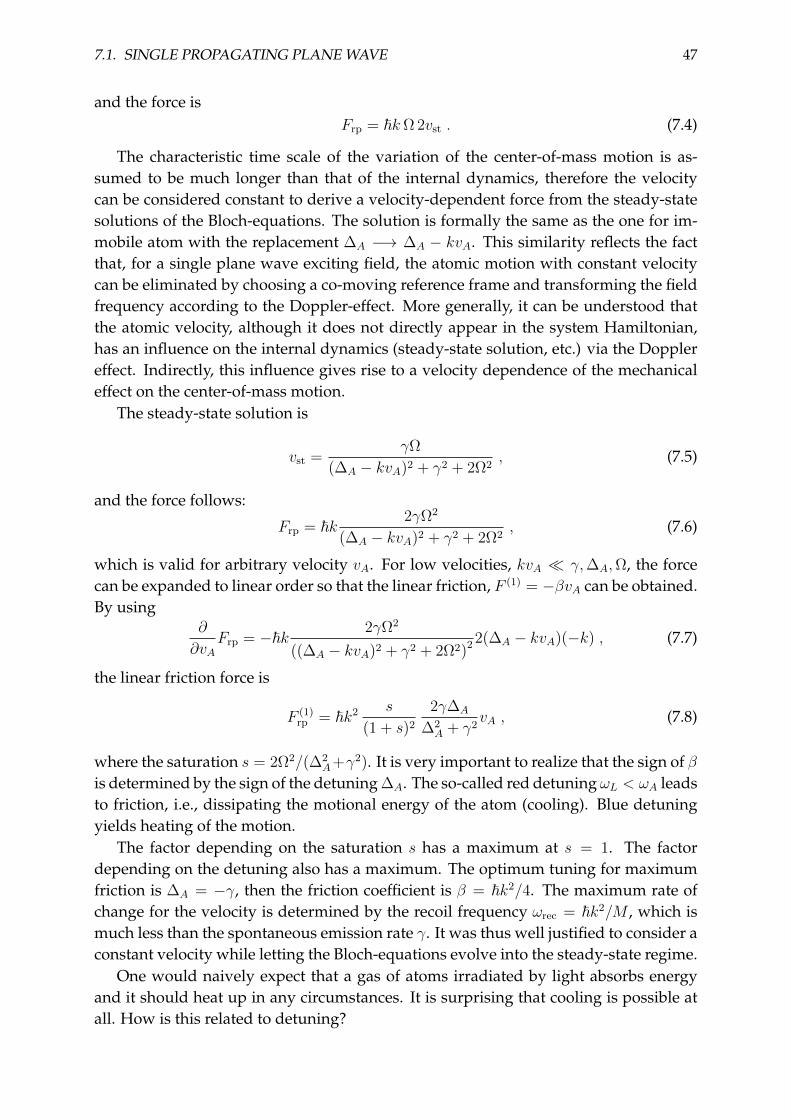
7.1. SINGLE PROPAGATING PLANE WAVE 47

and the force isFrp = ~kΩ 2vst . (7.4)

The characteristic time scale of the variation of the center-of-mass motion is as-sumed to be much longer than that of the internal dynamics, therefore the velocitycan be considered constant to derive a velocity-dependent force from the steady-statesolutions of the Bloch-equations. The solution is formally the same as the one for im-mobile atom with the replacement ∆A −→ ∆A − kvA. This similarity reflects the factthat, for a single plane wave exciting field, the atomic motion with constant velocitycan be eliminated by choosing a co-moving reference frame and transforming the fieldfrequency according to the Doppler-effect. More generally, it can be understood thatthe atomic velocity, although it does not directly appear in the system Hamiltonian,has an influence on the internal dynamics (steady-state solution, etc.) via the Dopplereffect. Indirectly, this influence gives rise to a velocity dependence of the mechanicaleffect on the center-of-mass motion.

The steady-state solution is

vst =γΩ

(∆A − kvA)2 + γ2 + 2Ω2, (7.5)

and the force follows:

Frp = ~k2γΩ2

(∆A − kvA)2 + γ2 + 2Ω2, (7.6)

which is valid for arbitrary velocity vA. For low velocities, kvA γ,∆A,Ω, the forcecan be expanded to linear order so that the linear friction, F (1) = −βvA can be obtained.By using

∂

∂vAFrp = −~k 2γΩ2

((∆A − kvA)2 + γ2 + 2Ω2)2 2(∆A − kvA)(−k) , (7.7)

the linear friction force is

F (1)rp = ~k2 s

(1 + s)2

2γ∆A

∆2A + γ2

vA , (7.8)

where the saturation s = 2Ω2/(∆2A+γ2). It is very important to realize that the sign of β

is determined by the sign of the detuning ∆A. The so-called red detuning ωL < ωA leadsto friction, i.e., dissipating the motional energy of the atom (cooling). Blue detuningyields heating of the motion.

The factor depending on the saturation s has a maximum at s = 1. The factordepending on the detuning also has a maximum. The optimum tuning for maximumfriction is ∆A = −γ, then the friction coefficient is β = ~k2/4. The maximum rate ofchange for the velocity is determined by the recoil frequency ωrec = ~k2/M , which ismuch less than the spontaneous emission rate γ. It was thus well justified to consider aconstant velocity while letting the Bloch-equations evolve into the steady-state regime.

One would naively expect that a gas of atoms irradiated by light absorbs energyand it should heat up in any circumstances. It is surprising that cooling is possible atall. How is this related to detuning?

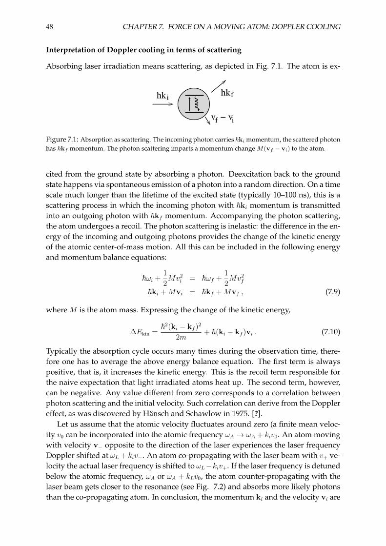
48 CHAPTER 7. FORCE ON A MOVING ATOM: DOPPLER COOLING

Interpretation of Doppler cooling in terms of scattering

Absorbing laser irradiation means scattering, as depicted in Fig. 7.1. The atom is ex-

hki

v − vf i

hkf

Figure 7.1: Absorption as scattering. The incoming photon carries ~ki momentum, the scattered photonhas ~kf momentum. The photon scattering imparts a momentum change M(vf − vi) to the atom.

cited from the ground state by absorbing a photon. Deexcitation back to the groundstate happens via spontaneous emission of a photon into a random direction. On a timescale much longer than the lifetime of the excited state (typically 10–100 ns), this is ascattering process in which the incoming photon with ~ki momentum is transmittedinto an outgoing photon with ~kf momentum. Accompanying the photon scattering,the atom undergoes a recoil. The photon scattering is inelastic: the difference in the en-ergy of the incoming and outgoing photons provides the change of the kinetic energyof the atomic center-of-mass motion. All this can be included in the following energyand momentum balance equations:

~ωi +1

2Mv2

i = ~ωf +1

2Mv2

f

~ki +Mvi = ~kf +Mvf , (7.9)

where M is the atom mass. Expressing the change of the kinetic energy,

∆Ekin =~2(ki − kf )

2

2m+ ~(ki − kf )vi . (7.10)

Typically the absorption cycle occurs many times during the observation time, there-fore one has to average the above energy balance equation. The first term is alwayspositive, that is, it increases the kinetic energy. This is the recoil term responsible forthe naive expectation that light irradiated atoms heat up. The second term, however,can be negative. Any value different from zero corresponds to a correlation betweenphoton scattering and the initial velocity. Such correlation can derive from the Dopplereffect, as was discovered by Hansch and Schawlow in 1975. [?].

Let us assume that the atomic velocity fluctuates around zero (a finite mean veloc-ity v0 can be incorporated into the atomic frequency ωA → ωA + kiv0. An atom movingwith velocity v− opposite to the direction of the laser experiences the laser frequencyDoppler shifted at ωL + kiv−. An atom co-propagating with the laser beam with v+ ve-locity the actual laser frequency is shifted to ωL−kiv+. If the laser frequency is detunedbelow the atomic frequency, ωA or ωA + kLv0, the atom counter-propagating with thelaser beam gets closer to the resonance (see Fig. 7.2) and absorbs more likely photonsthan the co-propagating atom. In conclusion, the momentum ki and the velocity vi are

7.2. SINGLE STANDING PLANE WAVE 49

ωA

ωL

ωL+ kv−

Lω − kv+ γ

vhk i v− +

Figure 7.2: Atomic resonance curve at ωA with width 2γ and Doppler-shifted driving frequencies asso-ciated with velocities v− and v+, respectively.

not independent in the actual scattering processes, and on average

〈kivi〉 ∼ 〈ki(v+ − v−)〉 < 0 . (7.11)

The outgoing photon momentum and the initial velocity are not correlated, 〈kfvi〉 =

0, therefore in Eq. (7.10) the second term is negative. Moreover it can dominate thefirst, recoil term, which leads to cooling. The kinetic energy reduction implies that theoutgoing photon must have a higher frequency than the incoming one.

7.2 Single standing plane wave

Two counter-propagating plane waves, which geometry was invoked above, form astanding wave provided the phases of the two beams are locked. This is not necessarythe case and than the forces exerted independently by the propagating plane wavescan simply be added. When there is a coherence between the beams, in a standingwave laser field mode, the atom-field interaction is substantially different.

In the compact form given in Eq. (5.2), the standing wave field corresponds to thatthere is no local phase, Φ ≡ 0, and only the spatially inhomogeneous Rabi-frequencyΩ(RA(t)) depends on time. The force now originates from the dipole force,

Fdip = ~∇Ω 2ust , (7.12)

which clearly shows the important difference inasmuch as the dispersive part of thesusceptibility ust appears in the force.

By contrast to the propagating plane wave case, here the Bloch matrix B in Eq. (7.3)depends on time. Although this specific problem can be solved for arbitrary velocitywith the continued fraction method, we will resort to a method which applies only tosmall velocities, however, which is a much more general approach.

As time dependence originates partly from motion, the time derivative is replacedby the hydrodynamic derivative and the solution is expanded into a power series ofthe velocity,

d

dt→ ∂

∂t+ v∇ and s = s(0) + s(1)v + . . . , (7.13)

50 CHAPTER 7. FORCE ON A MOVING ATOM: DOPPLER COOLING

respectively. Note that s(1) is a tensor mapping from the 3D space into the abstractspace of the Bloch vector, since all the spatial components of the velocity vx,y,z can havean effect on all the elements of the vector s = (u, v, w). The Bloch-equation becomes(

∂

∂t+ v∇

)(s(0) + s(1)v + . . .

)= B

(s(0) + s(1)v + . . .

)+ η . (7.14)

In steady-state the explicit time derivative vanishes, and one gets the hierarchy of equa-tions to different orders of the velocity v,

0 = Bs(0) + η , (7.15a)

(v∇)s(0) =(Bs(1)

)v , (7.15b)

and so on. The first line yields the steady-state for an atom in fixed position,

s(0) = −B−1η . (7.16)

This solution is needed to determine the solution in the next order,

s(1) = B−1∇ s(0) = −B−1∇ B−1η . (7.17)

In order to avoid the complications imposed by the tensors involved, we will usethis approach in a simplified system. We will consider an atom in the low saturationregime, s 1, where the w component can be eliminated assuming σz = −1/2 inEq. (5.7a): ⟨

˙σ⟩

= (i∆A − γ) 〈σ〉+ iΩ(R) . (7.18)

This is a simple linear equation. Physically this is an important limit of the atomic sys-tem, because it furnishes a microscopic model for linearly polarizable particles whichare ubiquitous in electrodynamics. The commutation relation for the associated quan-tum operator modifies to [

σ, σ†]

= −2σz ≈ 1 , (7.19)

i.e., the atom being close to the ground state behaves as a bosonic system, as if theatom were a harmonic oscillator whose excited states higher than the first one couldbe completely neglected.

Now the expansion method can be illustrated on Eq. (7.18) which is exempt fromthe tensorial character due to the Bloch-vector. The steady-state in zeroth and firstorder read

〈σ〉(0) =−iΩ(R)

i∆A − γ, (7.20a)

〈σ〉(1) =1

i∆A − γ∇−iΩ(R)

i∆A − γ= ∇Ω(R)

2∆Aγ − i(γ2 −∆2A)

(∆2A + γ2)2

, (7.20b)

As u = Re〈σ〉 follows from Eq. (5.8), the force to first order in velocity is

F(1)dip = 2~∇Ω(R)

(u(1)v

)= 2~∇Ω(R) ∇Ω(R)

2∆Aγ

(∆2A + γ2)2

v . (7.21)

7.2. SINGLE STANDING PLANE WAVE 51

For a plane wave Ω(R) = Ω cos(kR), in one dimension the friction force is

F(1)dip = 2~k2 sin2 kx

Ω2

∆2A + γ2

2∆Aγ

∆2A + γ2

v . (7.22)

The friction is maximum at the nodes of the standing wave, where the derivative of themode function is the maximum. On spatially averaging this inhomogeneous result,one gets back the same linear friction force as the one obtained in a propagating planewave. However, this equality holds only for the linear polarizability regime.

Chapter 8

Force fluctuations and momentumdiffusion

In this chapter we will consider the force terms which have vanishing mean value butgive rise to a momentum diffusion process.

8.1 Vacuum field force

The atom, regardless of being laser driven or not, is embedded in the electromagneticradiation field. The Hamiltonian accounting for the coupling of the atom to the elec-tromagnetic modes is

Hvac = −i~∑k,λ

gk,λ

(σ†ak,λe

ikRA − a†k,λσe−ikRA

). (8.1)

This coupling gives rise to a force exerted by the vacuum field. By definition, the forceis

Fvac = −∇Hvac = −∑k,λ

~kgk,λ

(σ†ak,λe

ikRA + a†k,λσe−ikRA

). (8.2)

To evaluate the vacuum force, we use the same separation of the vacuum field intofree field and radiated field components as previously in Chapter 3. The Heisenbergequations of motion for the field amplitudes are

ak,λ = −iωkak,λ + gk,λσe−ikRA , (8.3)

from which the formal solution follows

ak,λ(t) = ak,λ(0)e−iωkt + gk,λ

∫ t

0

dt′σ(t′)e−ikRAe−iωk(t−t′) . (8.4)

On inserting back this solution into the force, one gets two terms,

Fvac =−∑k,λ

~kgk,λ

(σ†(t)ak,λ(0)e−iωkteikRA + a†k,λ(0)σ(t)eiωkte−ikRA

)−∑k,λ

~kg2k,λ

∫ t

0

dt′(σ†(t)σ(t′)e−iωk(t−t′) + σ†(t′)σ(t)eiωk(t−t′)

). (8.5)

52

8.2. VACUUM FIELD FORCE FLUCTUTATIONS 53

The second term is identically zero since the terms belonging±k annihilate in the sum.Physically, the field radiated by the atom has no force acting back on it. Thus thevacuum field force is

Fvac = −∑k,λ

~kgk,λ

(σ†(t)ak,λ(0)e−iωkteikRA + a†k,λ(0)σ(t)eiωkte−ikRA

)(8.6)

The quantum mechanical mean value of this force is obviously zero. However, it makesa huge difference that the operator is not zero, hence there are non-vanishing higherorder moments which we are going to calculate in the following.

8.2 Vacuum field force fluctutations

For later convenience, we assume that there is a dominant carrier frequency ωL anddefine the slowly varying atomic operators σ and σ† in a frame rotating with this fre-quency. Let us study the second-order correlation of the vacuum field force,

〈Fvac(t1) Fvac(t2)〉 = ~2∑k1,λ1

∑k2,λ2

k1 k2 gk1,λ1gk2,λ2(⟨σ†(t1)ak1,λ1(t0)a†k2,λ2

(t0)σ(t2)⟩ei(k1−k2)RAe−i(ω1−ωL)t1 ei(ω2−ωL)t2

+⟨σ†(t1)ak1,λ1(t0)σ†(t2)ak2,λ2(t0)

⟩ei(k1+k2)RAe−i(ω1−ωL)t1 e−i(ω2−ωL)t2

+⟨a†k1,λ1

(t0)σ(t1)a†k2,λ2(t0)σ(t2)

⟩e−i(k1+k2)RAei(ω1−ωL)t1 ei(ω2−ωL)t2

+⟨a†k1,λ1

(t0)σ(t1)σ†(t2)ak2,λ2(t0)⟩e−i(k1−k2)RAei(ω1−ωL)t1 e−i(ω2−ωL)t2

).

(8.7)

In the last three lines, either the operator ak,λ(t0) is on the far most right or a†k,λ(t0) is onthe far most left in the bracket. Therefore all these terms vanish at zero temperature.In the first line, on using the commutation rule

[ak1,λ1(t0), a†k2,λ2

(t0)]

= δk1,k2δλ1,λ2 , onegets

〈Fvac(t1) Fvac(t2)〉 = ~2∑k,λ

k k g2k,λ

⟨σ†(t1)σ(t2)

⟩e−i(ωk−ωL)(t1−t2)

+ ~2⟨σ†(t1)f †(t2) f(t1)σ(t2)

⟩, (8.8)

wheref(t) =

∑k,λ

kgk,λak,λ(t0)eikRAe−i(ωk−ωL)t = −i∇ξ (8.9)

As f †(t2) contains only the operators a†k,λ(t0), its action on the bra state would be zero.Similarly, f(t1) is composed of the annihilation operators ak,λ(t0) and it maps the initialket state to zero. The problem is, however, that the commutation relation with theatomic operators σ and σ† is unknown. This can be calculated with the trick used oncefor the calculation of the quantum noise correlations of ξ at the end of Chap. 3. Let

54 CHAPTER 8. FORCE FLUCTUATIONS AND MOMENTUM DIFFUSION

us express the free field operators at t = t0 from the ones at t = t2 by propagating‘backward’ in time, i.e., using the formal solution in Eq. (3.4),

ak,λ(0) = ak,λ(t2)eiωkt2 + gk,λ

∫ t2

0

dt′σ(t′)e−ikRAei(ωk−ωL)t′ . (8.10)

Operators ak,λ(t2) and σ(t2) commute, since they are at equal times, thus

[ξ(t1), σ(t2)] = −∑k,λ

gk,λeikRAe−i(ωk−ωL)t1gk,λ

∫ t2

t0

dt′e−ikRAei(ωk−ωL)t′ [σ(t′), σ(t1)]x

= −∑k,λ

g2k,λ

∫ t2

t0

dt′ [σ(t′), σ(t2)] ei(ωk−ωL)(t′−t1)

≈ −θ(t2 − t1) [σ(t1), σ(t2)]∑k,λ

g2k,λ

∫ t2

t0

dt′ei(ωk−ωL)(t′−t1)

= −γθ(t2 − t1) [σ(t1), σ(t2)] , (8.11)

where we used the Markov-approximation. This expresses the fact that the noise oper-ators at time t1 commute with the system operators at a prior time t2 < t1. By contrast,at later times t2 > t1 the system operator involves the previous noise and then thecommutation relation becomes non-trivial.

Concerning the second term of Eq. (8.8), it follows that⟨σ†(t1)f †(t2) f(t1)σ(t2)

⟩∝ Θ(t2 − t1) Θ(t1 − t2) , (8.12)

which is zero except for precisely at t1 = t2. At his single point the commutator isnegligibly small with respect to the contribution of the first term of Eq. (8.8).

Finally we arrive at

〈Fvac(t1) Fvac(t2)〉 = ~2∑k,λ

k k g2k,λ

⟨σ†(t1)σ(t2)

⟩e−i(ω−ωL)(t1−t2) . (8.13)

The summation involves a broadband frequency range, therefore any finite time differ-ence |t1 − t2| > 1/ΩB, where ΩB is the reservoir bandwidth, makes the complex phasefactor average out the sum. Again, in the spirit of the Markov approximation,

〈Fvac(t1) Fvac(t2)〉 = ~2k2A γ

⟨σ†σ⟩ 2/5 0 0

0 2/5 0

0 0 1/5

δ(t1 − t2) . (8.14)

This force correlation function with the magnitude Drec can be identified with the dif-fusion coefficient of a classical stochastic process. The diffusion coefficient expressesthat the corresponding Brownian motion has a “stepsize” ~kA with a numerical factoraccounting for the projection onto the different cartesian directions, and random stepsoccur at the rate of the spontaneous emission, 2γ

⟨σ†σ⟩. That is the physical origin is

the recoil, accompanying each spontaneous emission event, into a random direction.

8.3. LASER FIELD FORCE FLUCTUATIONS 55

8.3 Laser field force fluctuations

One effect of the vacuum field modes was discussed in the previous chapter. There isa diffusion of the center-of-mass motion stemming from the random recoil followinga spontaneous emission, and this process is incorporated into the vacuum force termEq. (6.3b). This is not all: the noise due to coupling to the vacuum field penetratesthe system variables and therefore the force originating from the coherent laser fieldalso picks up a fluctuating character. Eq. (6.3a) presents the force due to the laser ir-radiation, having a linear dependence on the atomic polarization operators σ and σ†.Besides the mean value of the laser field force corresponding to the mean polarization,there is an additional diffusion from the quantum fluctuations of the atomic polar-ization. The fluctuations are of quantum nature originating from the coupling to theelectromagnetic radiation field in vacuum state, since the system is considered at zerotemperature. The second order autocorrelation function of the force operator involvesthe correlations such as

⟨δσ(t1)δσ†(t2)

⟩that can be calculated by invoking the quantum

regression theorem, as it was done to calculate the incoherent spectrum of the dipoleradiation in Sec. 5.3.

Here we will adopt a different, more direct approach which reveals some genericproperties of noise processes. In a frame rotating at the laser frequency, the Heisenbergequations of motion for the atomic operators read

˙σ = (i∆A − γ)σ − i2σzΩe−iΦ + Ξ(t) , (8.15a)

σz = −2γ(σz + 1/2) + iΩ(σ†e−iΦ − σeiΦ

)−Ξz(t) , (8.15b)

where Ξ(t) = 2σz(t)ξ(t) , Ξz(t) = σ†(t)ξ(t) + ξ†(t)σ(t) , (8.15c)

with ξ(t) =∑k,λ

gk,λak,λ(0)eikRAe−i(ωk−ωL)t . (8.15d)

The properties of the noise term are descibed by the second-order correlations derivedin Section 3.4.

⟨ξ(t1)ξ†(t2)

⟩=∑k1,λ1

∑k2,λ2

gk1,λ1gk2,λ2

⟨ak1,λ1(t0)a†k2,λ2

(t0)⟩e−i(ω1−ωL)t1ei(ω2−ωL)t2

=∑k,λ

g2k,λe

−i(ωk−ωL)(t1−t2) = γδ(t1 − t2) (8.16a)

〈ξ(t1)ξ(t2)〉 = 0 ,⟨ξ†(t1)ξ†(t2)

⟩= 0 ,

⟨ξ†(t1)ξ(t2)

⟩= 0 . (8.16b)

The linear Bloch equations can be integrated including the quantum noise, Ξ(t) andΞz(t), which represents an inhomogeneous driving term. Besides the decaying ho-mogeneous part, the general solution is a linear combination of the time integratednoise. The noise, evidently, does not contribute to the mean value, however, it has anon-vanishing second-order moment and thus leads to diffusion.

Let us solve this problem in the weak excitation limit, σz ≈ −12, where the Bloch-

equations decouple. The polarization obeys a simple linear equation which can be


integrated as

σ = e(i∆A−γ)tσ(0) + iΩe−iΦ∫ t

0

dt′e(i∆A−γ)(t−t′) −∫ t

0

dt′e(i∆A−γ)(t−t′)ξ(t′)

→ − iΩe−iΦ

i∆A − γ−∫ t

0

dt′e(i∆A−γ)(t−t′)ξ(t′) (8.17)

The quantum correlation of the atomic polarization is⟨σ(t1)σ†(t2)

⟩− 〈σ(t1)〉

⟨σ†(t2)

⟩=

=

∫ t1

0

dt′∫ t2

0

dt′′e(i∆A−γ)(t1−t′)e−(i∆A+γ)(t2−t′′)⟨ξ(t′)ξ†(t′′)

⟩=

∫ t1

0

dt′∫ t2

0

dt′′e(i∆A−γ)(t1−t′)e−(i∆A+γ)(t2−t′′)∑k,λ

g2k,λe

−i(ωk−ωL)(t′−t′′)

=∑k,λ

g2k,λe

(i∆A−γ)t1e−(i∆A+γ)t2

∫ t1

0

dt′e[−i(ωk−ωA)+γ]t′∫ t2

0

dt′′e[i(ωk−ωA)+γ]t′′

=∑k,λ

g2k,λ

(ωk − ωA)2 + γ2e−i(ωk−ωL)(t1−t2) . (8.18)

This result expresses a profound physical effect. Although the quantum noise sourceis supposed to be broadband, corresponding to the relevant frequency range of thevacuum field mode spectrum, the quantum noise associated with the polarization dy-namics is filtered through its Lorentz-type resonance curve. This latter has a width ofγ. The argument that the prefactor of the ‘fast oscillating’ exponential is slowly vary-ing function of the frequency ωk applies only for a frequency range well within thebandwidth γ. That is, the correlation function is strongly peaked around t1 ≈ t2 only ifthe time is resolved on a much larger scale than the natural lifetime 1/γ. However, thisis still a good resolution for the center-of-mass dynamics which takes place on a timescale of 1/ωrec 1/γ. As a consequence, the correlation can be considered a Dirac-δ onthis time scale, ⟨

σ(t1)σ†(t2)⟩− 〈σ(t1)〉

⟨σ†(t2)

⟩=

γ

∆2A + γ2

δ1/γ(t1 − t2) , (8.19)

where we explicitly indicate the physical ‘width’ of the Dirac-δ.

8.4 Diffusion from polarization noise

The dipole force correlation function is

〈δFdip(t1)δFdip(t2)〉 = ~2∇Ω ∇Ω⟨(δσ†(t1)e−iΦ(RA) + δσ(t1)eiΦ(RA)

) (δσ†(t2)e−iΦ(RA) + δσ(t2)eiΦ(RA)

)⟩=

= ~2∇Ω ∇Ω⟨σ(t1)σ†(t2)

⟩= ~2∇Ω ∇Ω

γ

∆2A + γ2

δ1/γ(t1 − t2) . (8.20)

8.5. OPTICAL MOLASSES, DOPPLER TEMPERATURE 57

In a one-dimensional, standing wave laser field, Ω(RA) = Ω cos kLx, the diffusioncoefficient is

Ddip = (~kL)2 γΩ2

∆2A + γ2

sin2 (kLx) . (8.21)

This diffusion is responsible for the spread of the momentum square, thus the increaseof the kinetic energy occurs in units of the recoil energy (~kL)2/M per spontaneousscattering event. This fact justifies again that the characteristic energy scale of thecenter-of-mass dynamics is determined by the recoil frequency.

Note that the recoil diffusion in such a laser field is

Drec =2

5(~kA)2 γΩ2

∆2A + γ2

cos2 (kLx) , (8.22)

being similar in order of magnitude. However, the two types of diffusion process havea maximum shifted in space. With respect to the dipole potential in such a laser field,

U =~∆AΩ2

∆2A + γ2

cos2 (kLx) , (8.23)

the recoil noise is maximum at the antinodes where the excited state population⟨σ†σ⟩

is maximum, while the dipole force fluctuations are maximum at the largest slope ofthe dipole potential.

The radiation pressure force correlation function can be similarly derived,

〈δFrp(t1)δFrp(t2)〉 = −~2Ω2∇Φ ∇Φ⟨(δσ†(t1)e−iΦ(RA) − δσ(t1)eiΦ(RA)

) (δσ†(t2)e−iΦ(RA) − δσ(t2)eiΦ(RA)

)⟩=

= ~2∇Φ ∇ΦΩ2⟨σ(t1)σ†(t2)

⟩= ~2∇Φ ∇Φ

γΩ2

∆2A + γ2

δ1/γ(t1 − t2) . (8.24)

In a one-dimensional propagating plane wave∇Φ = −kL, thus the diffusion reads

Drp = (~kL)2 γΩ2

∆2A + γ2

. (8.25)

8.5 Optical molasses, Doppler temperature

For proper setting of the laser field, the atoms undergo a frictional force damping themotional energy. The atoms irradiated from a pair of counter-propagating laser fieldsfrom each of the three spatial dimensions form what is called the optical molasses. Theatoms are not trapped in a potential, but move diffusively under the strong viscouseffect of the cooling laser beams. Since the friction is linear in velocity, the larger themean kinetic energy, the larger amount of heat is dissipated. This cooling process iscounteracted by the diffusion originating from the recoil diffusion and the one asso-ciated with the polarization fluctuations. The two processes are in balance at a givenvalue of the mean kinetic energy. In this stationary situation, by the equipartition the-orem, the kinetic energy is associated with a temperature.


Assume the atoms move in one dimension along a red detuned standing wave laserfield. Neglecting the localization around field antinodes, the friction can be approxi-mated by spatially averaging the result Eq. (7.22),

β =1

2~k2 2Ω2

∆2A + γ2

2 |∆A| γ∆2A + γ2

. (8.26)

The diffusion coefficient, also spatially averaged, reads

D =1

2

(1 +

2

5

)(~k)2 Ω2γ

∆2A + γ2

, (8.27)

from which the temperature, according to Eq. (6.27),

kBTDoppler ≈D

β=

7

10~γ

∆2A + γ2

2 |∆A| γ. (8.28)

The temperature is limited by the atomic linewidth. This is due to the fact that thedissipation channel is spontaneous emission. The velocity-dependence arises fromthe Doppler effect, finely tuning the resonance of width γ. The optimum detuningto minimize the temperature is ∆A = −γ. With this choice the temperature is aboutkBTDoppler ≈ ~γ, the so-called Doppler temperature. Numerically,

240µK Sodium145µK Rubidium124µK Cesium

. (8.29)

To a large surprise, the measurements yielded somewhat lower temperatures,moreover, the lowest temperature was obtained at a detuning ∆A = −3γ. These ob-servations indicated that there is a mechanism responisble for cooling other than theDoppler-cooling that we have studied so far. For a better understanding, one needs toconsider the multilevel structure of atoms.

Chapter 9

Polarization-gradient cooling

9.1 Radiation field with polarization gradient

Let us consider the field arising from two counterpropagating, monochromatic plane-wave modes having orthogonal linear polarizations. This configuration is called‘lin⊥lin’. The electric field, to be real, has a positive and negative frequency part,

E(z, t) = E (+)(z)e−iωLt + E (−)(z)eiωLt , (9.1)

with the two modesE (+)(z) = E0εe

ikz + E ′0ε′e−ikz . (9.2)

Let us shift the origin of the coordiante space to z → z+λ/8 for later convenience. Thepolarizations are ε = εx and ε′ = εy. For simplicity, the amplitudes are chosen to beequal, i.e., E0 = E ′0. The total amplitude can be expressed in various equivalent forms,

E (+)(z)/E0 = εx1 + i√

2(cos kz + i sin kz) + εy

1− i√2

(cos kz − i sin kz)

=εx + εy√

2(cos kz − sin kz) + i

εx − εy√2

(cos kz + sin kz) (9.3a)

= (1 + i)

(cos kz

εx − iεy√2

+ i sin kzεx + iεy√

2

). (9.3b)

The expression in the second line shows that the field is linearly polarized in the po-sitions where cos kz = ± sin kz. For tan kz = 1, which occurs with periodicity π, thepolarization is εx+εy√

2, while for π/2 shifted positions it is εx−εy√

2. Both directions make an

angle of π/4 with x and y. In the middle positions, i.e., kz = (n + 1/4)π, the field hasa circular polarization alternatively in the ε± directions. These are two basis vectors ofthe spherical coordinate system, defined as

ε+ = − 1√2

(εx + iεy) , (9.4a)

ε0 = εz , (9.4b)

ε− =1√2

(εx − iεy) . (9.4c)

59

60 CHAPTER 9. POLARIZATION-GRADIENT COOLING

In summary the field has a spatially dependent polarization. Any transition with agiven polarization is driven with spatially varying strength, hence the Rabi frequencyhas a gradient because of the varying polarization, not because of the varying inten-sity. At the same time, the atomic internal dynamics cannot be restricted to two levels,since the transitions with different rotational symmetry are excited by the laser field atdifferent positions.

9.2 Atomic multiplet transitions

In the spherical coordinate system defined by the unit ortho-normalized basis vectorsεq, q = ±, 0, the components of a vector can be expressed as,

r+ = − 1√2r sin θeiφ =

(4π

3

)1/2

rY1,1(θ, φ) (9.5a)

r0 = r cos θ =

(4π

3

)1/2

rY1,0(θ, φ) , (9.5b)

r− = − 1√2r sin θe−iφ =

(4π

3

)1/2

rY1,−1(θ, φ) (9.5c)

where YJ,M(θ, φ) are the spherical harmonics. Thus the position vector is

r =

(4π

3

)1/2

r∑

q=−1,0,1

εqY1,q(θ, φ) . (9.6)

The matrix elements of the dipole operator can be conveniently calculated in this basis

〈JeMe| er |JgMg〉 = 〈Je| er |Jg〉∑q

εq

(4π

3

)1/2 ∫dΩY ∗Je,Me

(θ, φ)Y1,q(θ, φ)YJg ,Mg(θ, φ)

= deg

√2Jg + 1

2Je + 1〈Jg100 | Je0〉

∑q

εq 〈Jg1Mgq | JeMe〉 , (9.7)

where we used the relation∫dΩY ∗Je,Me

(θ, φ)Y1,q(θ, φ)YJg ,Mg(θ, φ) = (−1)Me

∫dΩYJg ,MgY1,qYJe,−Me

=((−1)Me

)2(

(2Jg + 1) 3

4π(2Je + 1)

)1/2

〈Jg100 | Je0〉〈Jg1Mgq | JeMe〉 , (9.8)

and the definitiondeg = 〈Je| er |Jg〉 =

∫drr3R∗e,JeRg,Jg . (9.9)

Note that the radial functions depend on the multiplicity J in general (the Coulombproblem is an exception).

Thus the dipole operator for an atomic transition between multiplets can be writtenas

d = deg

√2Jg + 1

2Je + 1〈Jg100 | Je0〉

∑q=0,±1

(εqσq + ε∗qσ

†q

), (9.10)

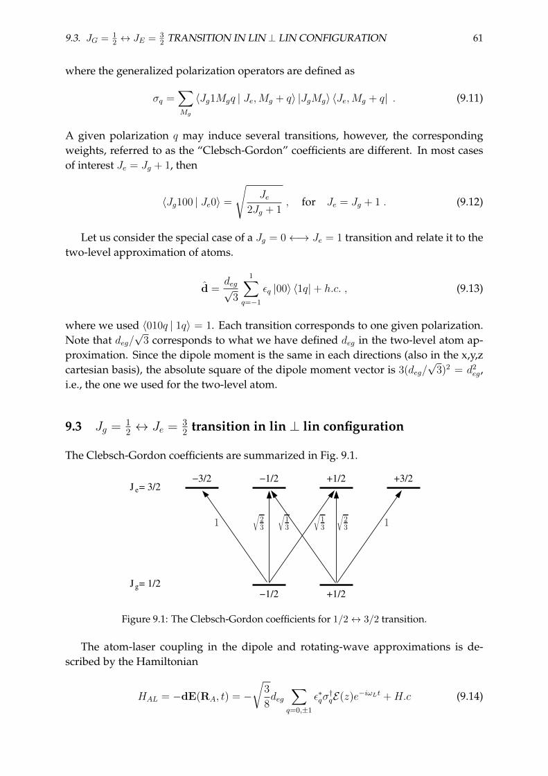
9.3. JG = 12 ↔ JE = 3

2 TRANSITION IN LIN ⊥ LIN CONFIGURATION 61

where the generalized polarization operators are defined as

σq =∑Mg

〈Jg1Mgq | Je,Mg + q〉 |JgMg〉〈Je,Mg + q| . (9.11)

A given polarization q may induce several transitions, however, the correspondingweights, referred to as the “Clebsch-Gordon” coefficients are different. In most casesof interest Je = Jg + 1, then

〈Jg100 | Je0〉 =

√Je

2Jg + 1, for Je = Jg + 1 . (9.12)

Let us consider the special case of a Jg = 0←→ Je = 1 transition and relate it to thetwo-level approximation of atoms.

d =deg√

3

1∑q=−1

εq |00〉〈1q|+ h.c. , (9.13)

where we used 〈010q | 1q〉 = 1. Each transition corresponds to one given polarization.Note that deg/

√3 corresponds to what we have defined deg in the two-level atom ap-

proximation. Since the dipole moment is the same in each directions (also in the x,y,zcartesian basis), the absolute square of the dipole moment vector is 3(deg/

√3)2 = d2

eg,i.e., the one we used for the two-level atom.

9.3 Jg = 12 ↔ Je = 3

2 transition in lin ⊥ lin configuration

The Clebsch-Gordon coefficients are summarized in Fig. 9.1.

e

J = 1/2g−1/2 +1/2

−1/2 +1/2 +3/2−3/2J = 3/2

1

√2

3

√1

3

√1

3

√2

31

1

Figure 9.1: The Clebsch-Gordon coefficients for 1/2↔ 3/2 transition.

The atom-laser coupling in the dipole and rotating-wave approximations is de-scribed by the Hamiltonian

HAL = −dE(RA, t) = −√

3

8deg

∑q=0,±1

ε∗qσ†qE(z)e−iωLt +H.c (9.14)


In a frame rotating at the laser frequency

H = −~∆A

∑Me

|Je,Me〉〈Je,Me|−√

3

8deg√

2E0

∑q=0,±1

1 + i√2ε∗qσ†q(ε− cos kz−iε+ sin kz)+H.c

= −~∆APe − ~Ω cos kz

(∣∣e−3/2

⟩ ⟨g−1/2

∣∣+1√3

∣∣e−1/2

⟩ ⟨g1/2

∣∣+H.c

)−

− i~Ω sin kz

(1√3

∣∣e1/2

⟩ ⟨g−1/2

∣∣+∣∣e3/2

⟩ ⟨g1/2

∣∣−H.c) (9.15)

where Ω is the Rabi frequency. The equations of motion for the mean values are readilyobtained. Denoting the means ρ(ai, bj) = 〈|ai〉〈bj|〉, where a, b = e, g and i, j are theZeeman-sublevel indices, the polarizations evolve as

ρ(g1/2, e3/2) = (i∆A − γ)ρ(g1/2, e3/2)− Ω sin kz(ρ(g1/2, g1/2)− ρ(e3/2, e3/2)

)− iΩ/

√3 cos kzρ(e−1/2, e3/2) ,

ρ(g1/2, e−1/2) = (i∆A − γ)ρ(g1/2, e−1/2) + iΩ/√

3 cos kz(ρ(g1/2, g1/2)− ρ(e−1/2, e−1/2)

)+ Ω sin kzρ(e3/2, e−1/2) ,

ρ(g−1/2, e1/2) = (i∆A − γ)ρ(g−1/2, e1/2)− Ω/√

3 sin kz(ρ(g−1/2, g−1/2)− ρ(e1/2, e1/2)

)− iΩ cos kzρ(e−3/2, e1/2) ,

ρ(g−1/2, e−3/2) = (i∆A−γ)ρ(g−1/2, e−3/2)+ iΩ cos kz(ρ(g−1/2, g−1/2)− ρ(e−3/2, e−3/2)

)+

Ω/√

3 sin kzρ(e1/2, e−3/2) .

The excited state populations evolve as

ρ(e3/2, e3/2) = −2γρ(e3/2, e3/2)− Ω sin kz(ρ(e3/2, g1/2) + ρ(g1/2, e3/2)

),

ρ(e1/2, e1/2) = −2γρ(e1/2, e1/2)− Ω√3

sin kz(ρ(e1/2, g−1/2) + ρ(g−1/2, e1/2)

),

ρ(e−1/2, e−1/2) = −2γρ(e−1/2, e−1/2) +iΩ√

3cos kz

(ρ(e−1/2, g1/2)− ρ(g1/2, e−1/2)

),

ρ(e−3/2, e−3/2) = −2γρ(e−3/2, e−3/2) + iΩ cos kz(ρ(e−3/2, g−1/2)− ρ(g−1/2, e−3/2)

).

Let us consider the weak driving limit realized by a Rabi frequency Ω muchsmaller than the detuning ∆A, or the linewidth γ. There is a small saturation s =

Ω2

∆2A+γ2

1, correspondingly, the population is dominantly in the ground states, i.e.,ρ(g±1/2, g±1/2) = O(1). The polarization associated with each transition is of first or-der in Ω, while the populations in the excited states is of second order in Ω. One cansystematically derive the leading order solution of the total system of equations by

9.3. JG = 12 ↔ JE = 3

2 TRANSITION IN LIN ⊥ LIN CONFIGURATION 63

considering the steady-state polarizations approximated by

ρ(g1/2, e3/2) ≈ − Ω

−i∆A + γsin kzΠ1/2 , (9.16a)

ρ(g1/2, e−1/2) ≈ i√3

Ω

−i∆A + γcos kzΠ1/2 , (9.16b)

ρ(g−1/2, e1/2) ≈ − 1√3

Ω

−i∆A + γsin kzΠ−1/2 , (9.16c)

ρ(g−1/2, e−3/2) ≈ iΩ

−i∆A + γcos kzΠ−1/2 , (9.16d)

where we have introduced the notation Π±1/2 ≡ ρ(g±1/2, g±1/2 for the ground statepopulations. Similarly, the excited state populations are given in leading order by

ρ(e3/2, e3/2) ≈ Ω2

∆2A + γ2

sin2 kzΠ1/2 , (9.17a)

ρ(e1/2, e1/2) ≈ 1

3

Ω2

∆2A + γ2

sin2 kzΠ−1/2 , (9.17b)

ρ(e−1/2, e−1/2) ≈ 1

3

Ω2

∆2A + γ2

cos2 kzΠ1/2 , (9.17c)

ρ(e−3/2, e−3/2) ≈ Ω2

∆2A + γ2

cos2 kzΠ−1/2 , (9.17d)

(9.17e)

The adiabatic dynamics of the ground state populations

The polarizations and the excited state populations evolve fast, the dynamicaltimescale is being given by ∆A and γ, therefore these variables of the system can be“slaved” to the slowly varying ground state populations by the relations Eq. (9.16) andEq. (9.17). An adiabatic Hamiltonian can be constructed from Eq. (9.15) by using theadiabatic solution for the polarizations with the populations retained as operators,

Had = ~∆A s1

3

[(1 + 2 cos2 kz)

∣∣g−1/2

⟩ ⟨g−1/2

∣∣+ (1 + 2 sin2 kz)∣∣g1/2

⟩ ⟨g1/2

∣∣] . (9.18)

This Hamiltonian is diagonal in the ground states∣∣g−1/2

⟩and

∣∣g1/2

⟩, which remain thus

eigenstates of the interacting system in the low saturation limit. Therefore there areno oscillations in the dynamics, only the corresponding eigenenergies are redefined,remarkably, the energies pick up a spatially dependent character. This simple structureof the Hamiltonian originates from the lack of coherent two-photon coupling betweenthe two ground states by the two laser fields. The adiabatic population redistributionbetween the ground states arises solely from decay processes via the virtually excited∣∣e±1/2

⟩states. The slow evolution of the master variables can be obtained from the


original Bloch-equations by using the adiabatic expressions for the slaved variables,

Π−1/2 = iΩ cos kz(ρ(g−1/2, e−3/2)− c.c.

)+

Ω√3

sin kz(ρ(g−1/2, e1/2) + c.c.

)+ 2γ

(ρ(e−3/2, e−3/2) +

2

3ρ(e−1/2, e−1/2) +

1

3ρ(e1/2, e1/2)

)= −2γ s cos2 kzΠ−1/2 −

1

32γ s sin2 kzΠ−1/2

+ 2γ s

(cos2 kzΠ−1/2 +

2

3

1

3cos2 kzΠ1/2 +

1

3

1

3sin2 kzΠ−1/2

)= −2γ s

(2

9sin2 kzΠ−1/2 −

2

9cos2 kzΠ1/2

)≈ −4γ s

9

(Π−1/2 − cos2 kz

), (9.19a)

where in the last step we used Π−1/2 +Π1/2 = 1−O(s). For the other ground state |1/2〉,the derivation follows analogously and leads to

Π+1/2 = −4γ s

9

(Π1/2 − sin2 kz

). (9.19b)

The stationary solution reads

Πst±1/2 =

sin2 kz

cos2 kz+O(s) . (9.20)

This result reflects the effect of optical pumping: the population is irreversibly transferedinto the state

∣∣g−1/2

⟩under the effect of a field with ε− polarization and, reversely, it is

transfered into∣∣g+1/2

⟩in a ε+ polarized driving field. The reason is that the system is

trapped, when the field is ε− polarized, in the∣∣g−1/2

⟩↔∣∣e−3/2

⟩transition. Meanwhile,

the system leaks out from the state∣∣g+1/2

⟩via the state

∣∣e−1/2

⟩, this latter spontaneously

decaying into∣∣g−1/2

⟩. This happens in the positions kz = 0, and the reverse optical

pumping process takes place in the positions kz = π/2.It follows from the differential equations (9.19) that the time scale of this optical

pumping is about (s0γ)−1, much longer than the decay time of the excited states andthat of the polarizations (γ−1). As we learned from the mechanism of Doppler cooling,some non-adiabatic evolution of the internal degrees of freedom is needed to producevelocity dependent forces. For a two-level atom the only time scale characteristic ofthe internal dynamics was γ−1, and velocities as small as kv γ can induce closelyadiabatic variation of the σ operators. By contrast, here we found that the adiabaticlimit is reached at much slower velocities, kv sγ. As a consequence, the coolingmechanism, which we will refer to as polarization gradient cooling, remains efficient formuch lower velocities.

9.4 The Sisyphus-cooling effect

For an atom at rest, the populations reach the local values cos2 kz and sin2 kz in thestate

∣∣g−1/2

⟩and

∣∣g1/2

⟩, respectively. Note that the larger population can be found

in the state having lower energy. Optical pumping in this scheme transfers thus the

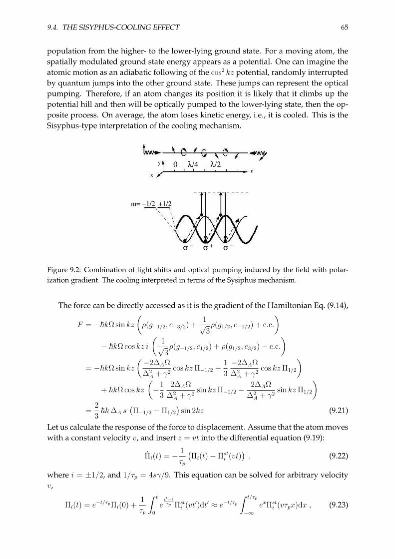
9.4. THE SISYPHUS-COOLING EFFECT 65

population from the higher- to the lower-lying ground state. For a moving atom, thespatially modulated ground state energy appears as a potential. One can imagine theatomic motion as an adiabatic following of the cos2 kz potential, randomly interruptedby quantum jumps into the other ground state. These jumps can represent the opticalpumping. Therefore, if an atom changes its position it is likely that it climbs up thepotential hill and then will be optically pumped to the lower-lying state, then the op-posite process. On average, the atom loses kinetic energy, i.e., it is cooled. This is theSisyphus-type interpretation of the cooling mechanism.

10.4. MECHANICAL FORCE 67

σ − σ −

x

y λ/4 λ/2

σ +

m= −1/2 +1/2

0

Figure 10.2: Combination of light shifts and optical pumping induced by the field withpolarization gradient. The cooling interpreted in terms of the Sysiphus mechanism.

Figure 9.2: Combination of light shifts and optical pumping induced by the field with polar-ization gradient. The cooling interpreted in terms of the Sysiphus mechanism.

The force can be directly accessed as it is the gradient of the Hamiltonian Eq. (9.14),

F = −~kΩ sin kz

(ρ(g−1/2, e−3/2) +

1√3ρ(g1/2, e−1/2) + c.c.

)− ~kΩ cos kz i

(1√3ρ(g−1/2, e1/2) + ρ(g1/2, e3/2)− c.c.

)= −~kΩ sin kz

(−2∆AΩ

∆2A + γ2

cos kzΠ−1/2 +1

3

−2∆AΩ

∆2A + γ2

cos kzΠ1/2

)+ ~kΩ cos kz

(−1

3

2∆AΩ

∆2A + γ2

sin kzΠ−1/2 −2∆AΩ

∆2A + γ2

sin kzΠ1/2

)=

2

3~k∆A s

(Π−1/2 − Π1/2

)sin 2kz (9.21)

Let us calculate the response of the force to displacement. Assume that the atom moveswith a constant velocity v, and insert z = vt into the differential equation (9.19):

Πi(t) = − 1

τp

(Πi(t)− Πst

i (vt)), (9.22)

where i = ±1/2, and 1/τp = 4sγ/9. This equation can be solved for arbitrary velocityv,

Πi(t) = e−t/τpΠi(0) +1

τp

∫ t

0

et′−tτp Πst

i (vt′)dt′ ≈ e−t/τp∫ t/τp

−∞exΠst

i (vτpx)dx , (9.23)


where the initial transient is removed. From the integral∫dx ex cos ax =

ex(cos ax+ a sin ax)

1 + a2, (9.24)

on identifying a = 2kvτp, one arrives at

Π± =1

2∓ 1

2

cos 2kvt+ 2kvτp sin 2kvt

1 + (2kvτp)2 . (9.25)

By using the force in Eq. (9.21), the velocity dependence is obtained,

F (v) =2

3~k∆A s

sin 4kvt+ 4kvτp sin2 2kvt

1 + (2kvτp)2 . (9.26)

Assuming that the atom passes through several wavelength during the time τp, thisinstantaneous force can be averaged over the position, which yields

F (v) =2

3~k2 ∆A s τp

v

1 +(vvc

)2 , (9.27)

where vc = 12kτp

is a characteristic velocity corresponding to the maximum of the forceand it also defines the velocity capture range. The velocity dependent force amountsto friction if the detuning is negative, i.e., ∆A < 0.

The maximum friction coefficient exceeds that of the Doppler cooling scheme by afactor of 1/s, however, the velocity capture range is smaller by a factor of s. Thus thisefficient cooling mechanism operates at low velocities. The friction force depends onlyweakly on s (in higher order powers of v), which shows that the friction cooling ceasesto work when the atom gets trapped in one of the potential wells given by the internalenergy expression Eq. (9.18). The momentum uncertainty arises from the randomnessof the direction of the last scattered photon. The limiting temperature thus is the recoiltemperature kBTrec = ~2k2/2M .

Chapter 10

Basic methods in laser cooling andtrapping

In this chapter we review the basic principles of the most common techniques usednowadays in the laboratories. The magneto-optical trapping (MOT) is the standardmethod to produce cold atomic sample with high density and large atom numbers.This trap has a mechanism which simultaneously confines in space and cools theatoms. The sideband cooling method can be applied to trapped atoms, eventually ina quantized center-of-mass motional state, and results in very low temperatures wellbelow the recoil limit.

10.1 Magneto-optical trapping

The interaction of atoms with a magnetic field via the magnetic moment of atoms hasnot been previously included in the theory which was based on the electric dipoleapproximation. This higher order interaction can be taken into account by the Hamil-tonian term

H = −µB . (10.1)

The atomic magnetic moment isµ = gFµBF , (10.2)

i.e., the product of the Bohr-magneton µB = e~/2me = 9.3×10−24J/T , the Lande-factorgF , and the quantum operator F associated with the total angular momentum of theatom. Let us assume that the atom moves very slowly on the length scale character-izing the magnetic field variation. In that case the moving atom adiabatically followsan eigenstate of the z component of the angular momentum where the orientation ofthe quantization axis is alway defined parallel with the direction of the local magneticfield. Therefore the scalar product can be replaced and the force acting on an atom inan inhomogeneous static magnetic field is

F = gFµBM ∇|B(R)| , (10.3)

where M is the angular momentum projection on the direction of the local magneticfield. The atomic states are characterized by the total electron spin S, the total orbital

67

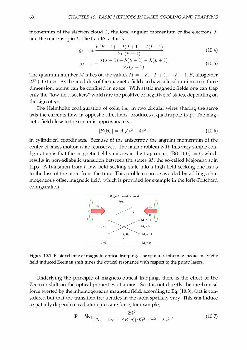
68 CHAPTER 10. BASIC METHODS IN LASER COOLING AND TRAPPING

momentum of the electron cloud L, the total angular momentum of the electrons J ,and the nucleus spin I . The Lande-factor is

gF = gjF (F + 1) + J(J + 1)− I(I + 1)

2F (F + 1)(10.4)

gJ = 1 +J(J + 1) + S(S + 1)− L(L+ 1)

2J(J + 1)(10.5)

The quantum number M takes on the values M = −F,−F + 1, . . . F − 1, F , altogether2F + 1 states. As the modulus of the magnetic field can have a local minimum in threedimension, atoms can be confined in space. With static magnetic fields one can traponly the “low-field seekers” which are the positive or negative M states, depending onthe sign of gF .

The Helmholtz configuration of coils, i.e., in two circular wires sharing the sameaxis the currents flow in opposite directions, produces a quadrupole trap. The mag-netic field close to the center is approximately

|B(R)| = A√ρ2 + 4z2 , (10.6)

in cylindrical coordinates. Because of the anisotropy the angular momentum of thecenter-of-mass motion is not conserved. The main problem with this very simple con-figuration is that the magnetic field vanishes in the trap center, |B(0, 0, 0)| = 0, whichresults in non-adiabatic transition between the states M , the so-called Majorana spinflips. A transition from a low-field seeking state into a high field seeking one leadsto the loss of the atom from the trap. This problem can be avoided by adding a ho-mogeneous offset magnetic field, which is provided for example in the Ioffe-Pritchardconfiguration.

M = −1e

M = 0e

M = +1e

M = 0g

ω L

ω L

σ +

I

ω L

σ −

I

J=0

J=1

z

B(z)

Magneto−optikai csapda

Figure 10.1: Basic scheme of magneto-optical trapping. The spatially inhomogeneous magneticfield induced Zeeman shift tunes the optical resonance with respect to the pump lasers.

Underlying the principle of magneto-optical trapping, there is the effect of theZeeman-shift on the optical properties of atoms. So it is not directly the mechanicalforce exerted by the inhomogeneous magnetic field, according to Eq. (10.3), that is con-sidered but that the transition frequencies in the atom spatially vary. This can inducea spatially dependent radiation pressure force, for example,

F = ~kγ2Ω2

(∆A − kv − µ′B(R)/~)2 + γ2 + 2Ω2, (10.7)

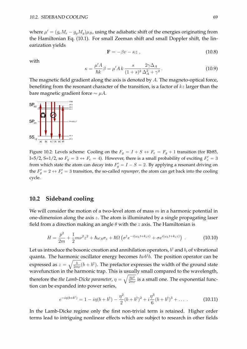
10.2. SIDEBAND COOLING 69

where µ′ = (geMe − ggMg)µB, using the adiabatic shift of the energies originating fromthe Hamiltonian Eq. (10.1). For small Zeeman shift and small Doppler shift, the lin-earization yields

F = −βv − κz , (10.8)

withκ =

µ′A

~kβ = µ′Ak

s

(1 + s)2

2γ∆A

∆2A + γ2

. (10.9)

The magnetic field gradient along the axis is denoted by A. The magneto-optical force,benefiting from the resonant character of the transition, is a factor of kz larger than thebare magnetic gradient force ∼ µA.

Figure 10.2: Levels scheme: Cooling on the Fg = I + S ↔ Fe = Fg + 1 transition (for Rb85,I=5/2, S=1/2, so Fg = 3 ↔ Fe = 4). However, there is a small probability of exciting F ′e = 3

from which state the atom can decay into F ′g = I − S = 2. By applying a resonant driving onthe F ′g = 2 ↔ F ′e = 3 transition, the so-called repumper, the atom can get back into the coolingcycle.

10.2 Sideband cooling

We will consider the motion of a two-level atom of mass m in a harmonic potential inone-dimension along the axis z. The atom is illuminated by a single propagating laserfield from a direction making an angle θ with the z axis. The Hamiltonian is

H =p2

2m+

1

2mν2z2 + ~ωAσz + ~Ω

(σ†e−i(ωLt+kzz) + σei(ωLt+kzz)

). (10.10)

Let us introduce the bosonic creation and annihilation operators, b† and b, of vibrationalquanta. The harmonic oscillator energy becomes ~νb†b. The position operator can be

expressed as z =√

~2mν

(b + b†). The prefactor expresses the width of the ground statewavefunction in the harmonic trap. This is usually small compared to the wavelength,

therefore the the Lamb-Dicke parameter, η =√

~k22mν

is a small one. The exponential func-tion can be expanded into power series,

e−iη(b+b†) = 1− iη(b+ b†)− η2

2(b+ b†)2 + i

η3

6(b+ b†)3 + . . . . (10.11)

In the Lamb-Dicke regime only the first non-trivial term is retained. Higher orderterms lead to intriguing nonlinear effects which are subject to research in other fields

70 CHAPTER 10. BASIC METHODS IN LASER COOLING AND TRAPPING

of quantum optics. The Hamiltonian in interaction picture reads

Hint = −i~Ω η[(σ†e−i∆At − σei∆At

) (be−iνt + b†eiνt

)]. (10.12)

For the most efficient sideband cooling, the laser has to be tuned one vibrationalquantum below the atomic resonance, i.e., ωL = ωA − ν. In the interaction pictureHamiltonian some of the terms become time independent (or slowly oscillating in caseof near resonance, ∆A ≈ −ν), the remaining ones rotate at least with an angular fre-quency of 2ν. When the vibrational frequency is much larger than any other frequencyin the dynamical system, that is, the effective Rabi frequency ηΩ and the spontaneousdecay rate γ, the system is in the resolved sideband limit, and the rotating terms can beneglected (secular approximation). The effective Hamiltonian simplifies to

Hint = −i~Ω (σ†b+ b†σ) . (10.13)

The vibrational motion of the atom in the trap can be dissipated via the spontaneousemission channel. This process will be described in the low saturation limit, when theatom is hardly excited and σz can be replaced by the c-number −1

2. The operators σ

and σ† formally are considered bosonic operators. One gets a simple set of coupledlinear differential equations

b = −ηΩσ , (10.14a)

σ = −γσ + ηΩb+ ξ , (10.14b)

where ξ is the quantum noise associated with the decay process. The eigenfrequenciesof the linear system are

λ± = −γ2±√(γ

2

)2

− (ηΩ)2 ≈ −γ2± γ

2∓ (ηΩ)2

γ+ γO

((ηΩ)

γ

)4

, (10.15)

where, in the approximation, we considered the overdamped limit, ηΩγ 1. The vibra-

tional mode is damped with a characteristic rate (ηΩ)2

γ.

Documents

Domokos Peter´ April 19, 2016