Embed Size (px)
Citation preview

Domain Theory, Computational Domain Theory, Computational Geometry and Differential Calculus Geometry and Differential Calculus
Abbas EdalatImperial College London
www.doc.ic.ac.uk/~ae
With contributions from Andre Lieutier, Ali Khanban, Marko Krznaric and Dirk Pattinson
First SQU Workshop on Topology and its ApplicationsDecember 2004
2
First rudimentary notion of a real numberFirst rudimentary notion of a real number
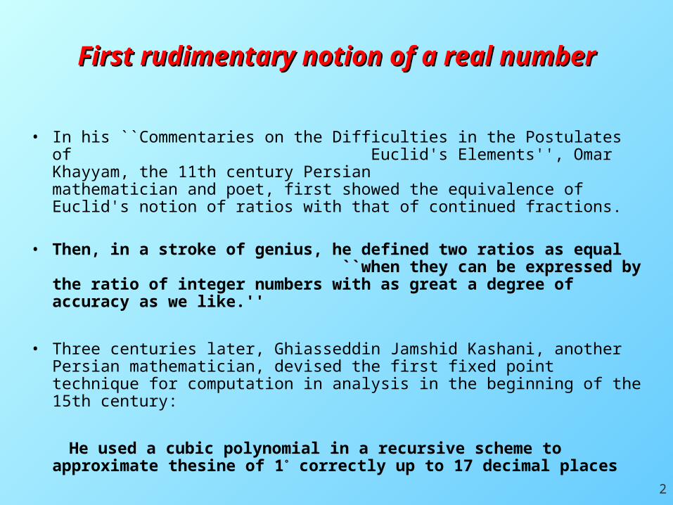
• In his ``Commentaries on the Difficulties in the Postulates of Euclid's Elements'', Omar Khayyam, the 11th century Persian mathematician and poet, first showed the equivalence of Euclid's notion of ratios with that of continued fractions.
• Then, in a stroke of genius, he defined two ratios as equal ``when they can be expressed by the ratio of integer numbers with as great a degree of accuracy as we like.''
• Three centuries later, Ghiasseddin Jamshid Kashani, another Persian mathematician, devised the first fixed point technique for computation in analysis in the beginning of the 15th century:
He used a cubic polynomial in a recursive scheme to approximate thesine of 1° correctly up to 17 decimal places

3
Computational Model for Classical Computational Model for Classical SpacesSpaces
XClassical Space
x
DXDomain
{x}
• Research project since 1993: Reconstruct mathematical analysis in an order-theoretic setting
• Embed classical spaces into the set of maximal elements of suitable partially ordered sets, called domains:

4
Computational Model for Classical Computational Model for Classical SpacesSpaces
• Applications:
Fractal Geometry
Measure & Integration Theory: Generalized Riemann Integration
Topological Representation of Spaces
Exact Real Arithmetic
Computational Geometry and Solid Modelling
Differential Calculus
Quantum Computation

5
Continuous Scott DomainsContinuous Scott Domains
• A directed complete partial order (dcpo) is a poset (A, ⊑) , in which every directed set {ai | iI } A has a sup or lub supiI ai
• The way-below relation in a dcpo is defined by:a ≪ b iff for all directed subsets {ai | iI }, the relation b sup⊑ iI ai implies that there exists i I such that a ⊑ ai
• If a ≪ b then a gives a finitary approximation to b
• B A is a basis if for each a A , {b B | b ≪ a } is directed with lub a
• A dcpo is (-)continuous if it has a (countable) basis
• A dcpo is bounded complete if every bounded subset has a lub
• A continuous Scott Domain is an -continuous bounded complete dcpo

6
Continuous functionsContinuous functions
• The Scott topology of a dcpo has as closed subsets downward closed subsets that are closed under the lub of directed subsets, usually only T0.
• Proposition. If D is a dcpo then f:D D is Scott continuous iff
• (i) f is monotone, i.e. f(x) f(y) if x y, and⊑ ⊑• (ii) f preserves sups of directed subsets, i.e. for any directed set
AD, we have: supaA f(a) = f(supA)
• Fact. The Scott topology on a continuous dcpo A with basis B has basic open sets {a A | b ≪ a } for each b B.

7
• Let IR={ [a,b] | a, b R} {R}
• (IR, ) is a bounded complete dcpo with R as bottom: supiI ai = iI ai
• a ≪ b ao b
• (IR, ⊑) is -continuous:countable basis {[p,q] | p < q & p, q Q}
• (IR, ⊑) is, thus, a continuous Scott domain.
• Scott topology has basis:↟a = {b | ao b} x {x}
R
I R
• x {x} : R IR an embedding
• We identify {x} with x
The Domain of nonempty compact The Domain of nonempty compact Intervals of Intervals of RR

8
Continuous FunctionsContinuous Functions
• Scott continuous f:[0,1]n IR is given by lower and upper semi-continuous functions f -, f +:[0,1]n R with f(x)=[f -(x),f +(x)]
• f : [0,1]n R, f C0[0,1]n, has continuous extension i(f ): [0,1]n IR x {f (x)}
• Scott continuous maps [0,1]n IR with: f ⊑ g x R . f(x) ⊑ g(x)is another continuous Scott domain.
• The function space [0,1]n IR is a continuous Scott domain. : C0[0,1]n ↪ ( [0,1]n IR), with f i(f) is a topological embedding into a proper subset of maximal elements of [0,1]n IR .
• We identify x and {x}, also f and i(f)

9
Step FunctionsStep Functions• Single-step function:
a↘b : [0,1]n IR, with a I[0,1]n, b=[b-,b+] IR:
b x ao x otherwise
• Lubs of finite and bounded collections of single- step functions f= sup1in(ai ↘ bi) are called step functions with N(f):= n (number of pieces)
• Step functions with ai, bi rational intervals give a basis for [0,1]n IR. They are used to approximate C0 functions.

10
Step Functions-An Example in RStep Functions-An Example in R
0 1
R
b1
a3
a2
a1
b3
b2

11
Refining the Step FunctionsRefining the Step Functions
0 1
R
b1
a3
a2
a1
b3
b2
12
Kleene’s Fixed Point TheoremKleene’s Fixed Point Theorem
• Theorem. If D is a dcpo with bottom (least element) d0 and if f : D D is Scott continuous then f has a least fixed point given by supiN f i(d0)
13
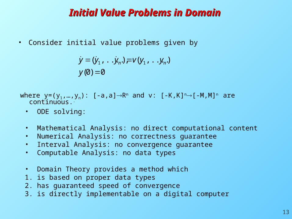
Initial Value Problems in Domain Initial Value Problems in Domain
0)0(
),....,(),....,( 11
y
yyvyyy nn
• Consider initial value problems given by
where y=(y1,…,yn): [-a,a]Rn and v: [-K,K]n[-M,M]n are continuous..
• ODE solving:
• Mathematical Analysis: no direct computational content• Numerical Analysis: no correctness guarantee• Interval Analysis: no convergence guarantee• Computable Analysis: no data types • Domain Theory provides a method which1. is based on proper data types2. has guaranteed speed of convergence3. is directly implementable on a digital computer

14
Picard's Classical TheoremPicard's Classical Theorem
• Proof: For y: [-a, a] [-K, K]n let Pv(y): [-a, a] [-K, K]n with
n1,.....,ifor )y,....,(yvy n1ii
)dty,...,(yvx:(y))(P n1
x
o iiv
• Standard assumption: v: [-K, K]n [-M, M]n and aM ≤K.
• Theorem: Suppose v is Lipschitz: |v(x) - v(y)| ≤ L |x – y| for some L > 0 and all x, y [-K, K]n. then, there exists a unique y: [-a, a] [-K, K]n with
By Banach's fixed point theorem, the sequence yk defined by y0 = any initial continuous function, and yk+1 = Pv(yk) converges to the unique fixed point.

15
Translation to Domain Theory: Road Translation to Domain Theory: Road mapmap
• Formulate the problem as fixed point equation over [-a,a]I[-K,K]n
• Apply Kleene's Theorem to obtain the least fixed point
• Relate domain-theoretic fixed points to the classical problem
• Show that the computations restrict to bases of the involved domains.
• Furthermore, we give: (i) Estimates on the speed of convergence (ii) Estimates on the (algebraic) complexity of the problem.

16
Translation to Domain Theory: Translation to Domain Theory: SolutionsSolutions
• Interval valued approximations to the solution:
• S = { y: [-a, a] I[-K, K]n | y Scott continuous} where
• I[-K, K]n = {A | A [-K, K]n is a compact rectangle} is the sub-domain of rectangles contained in [-K, K]n with reverse inclusion.
• The order on S is pointwise:
• If f, g S then f ⊑ g iff f(x) ⊑ g(x) for all x [-a, a].

17
Translation into Domain Theory: Vector Translation into Domain Theory: Vector FieldField
• Computing v(y) requires vector fields with interval input:
• V= { u: I[-K, K]n I[-M, M]n | u Scott continuous } with pointwise ordering
• Relationship to Classical Vector Fields: Extensions
• u V extends a classical v: [-K, K]n [-M, M]n if
• u({x}) = { v(x) } for all x [-K, K]n.
• The greatest or canonical extension of v is given by
Iv: I[-K, K]n I[-M, M]n with ((Iv)(A))i =vi[A]
18
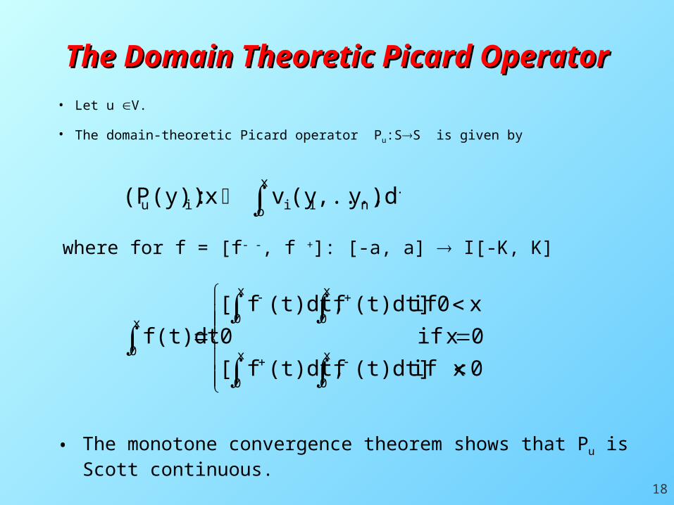
The Domain Theoretic Picard The Domain Theoretic Picard OperatorOperator
where for f = [f- -, f +]: [-a, a] I[-K, K]
)dty,...,(yvx:(y))(P n1
x
o iiu
• Let u V.
• The domain-theoretic Picard operator Pu:SS is given by
• The monotone convergence theorem shows that Pu is Scott continuous.
x
0 x
0
x
0
x
0
x
0
0 xif (t)dt]f(t)dt,f[
0 xif 0
x0 if (t)dt]f(t)dt,f[
f(t)dt

19
Relationship to the Classical ProblemRelationship to the Classical Problem
• Assume u is an extension of v: [-K, K]n [-M, M]n.
• Suppose y is the least fixed point of Pu
• Every solution f satisfies y ⊑ f
• If y = [y-, y+] and y- = y+, then y- is the unique solution.
• That is, we look for fixed points of width 0:
• For (A1, …..,An) I[-K, K]n, we write Ai = [Ai
-, Ai+] and define the width of A by
• w(A)=max{Ai+-Ai
- | 1≤i≤n}
• w(f)=sup{w(f(x))| x[-a,a]}

20
The Lipschitz CaseThe Lipschitz Case
• Recall: The classical proof assumes that v is Lipschitz.
• Suppose u is interval Lipschitz, that is
• w(u(x)) ≤L w(x) for all x I[-K, K]n.
• Then w(Pu(y)) ≤ a L w(y) for all y S.
• Assuming aL < 1 (which can be actually removed), we obtain
• Theorem:
y0 = [-K, K]n and yk+1 = Pu(yk). Then
y = sup kN yk satisfies Pu(y) = y and w(y) = 0.
• In particular, y - = y+ is the unique solution.

21
Approximations of the Vector FieldApproximations of the Vector Field
• Proposition: The map P: V→(S→S) with u→ Pu is Scott continuous.
• This allows us to use approximations of the vector field to obtain the solution:
. Then y = sup k N yk satisfies Pu(y) =y and w(y) = 0.
Speed of Convergence:
• If aL < c < 1 and d(u, uk) < 2Mck (c - aL), then w(yk) ≤ck w(y0), where
niiii
nkk
IRBA,for n}i1|:BA||,BAmax{|B)d(A,
:distance Hausdorff with the}K]I[-K, x| (x))u),sup{d(u(x))ud(u,
)(yPy ku1k k• Theorem: Suppose u = supk uk and y0 = [-K, K]n and

22
Restrinting to a BaseRestrinting to a Base• Let a,K,MQ.
• Denote the class of rational step functions I[-K,K]n→I[-M,M]n by VQ.
• We also have the class SL Q
of rational piecewise linear step functions
f:[-a,a]→I[-K,K]n
We again put N(f) = number of pieces in f In the above example N(f)=3
23
Computing with SComputing with SLLQQ and V and VQQ
• Pu restricts to the base:
• Suppose u VQ and y SLQ then:
• The map u(y) is piecewise constant, hence Pu(y) SLQ Pu(y) SL
Q .
• Pu(y) can be computed in time O(N(u)N(y)), i.e.
• N(Pu(y)) O(N(u)N(y)).

24
SummarySummary
• Suppose u = supk uk with uk VQ , y0= [-K, K]n and then
)(yPy ku1k k
• yk SLQ for all k N
• y = supk yk has width 0 and is the unique solution
• w(yk) O(ck) if d(u, uk) O(ck).
• Given an elementary function u, one can use continued fractions for to obtain uk with the above properties..
• These properties are preserved in an implementation using rational arithmetic.

25
PART II: A Domain-Theoretic Model for PART II: A Domain-Theoretic Model for Differential CalculusDifferential Calculus
• Overall Aim: Synthesize Computer Science with Differential Calculus
• Plan of the talk:1. Primitives of continuous interval-valued function in Rn
2. Derivative of a continuous function in Rn
3. Fundamental Theorem of Calculus for interval-valued functions in Rn
4. Domain of C1 functions in Rn
5. Inverse and implicit functions in domain theory

26
• For a = [a-, a+] IR, b = [b-, b+] IR,and * { +, –, } we have:
a * b = { x*y | x a, y b }
For example:
• a + b = [a- + b-, a+ + b+]
• Recall that for real x, we identify {x} with x.
Operations in Interval ArithmeticOperations in Interval Arithmetic
27
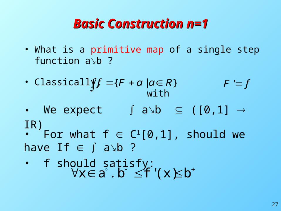
Basic Construction n=1Basic Construction n=1
• What is a primitive map of a single step function a↘b ?
• Classically, with }|{ RaaFf fF '
• We expect a↘b ([0,1] IR)
• For what f C1[0,1], should we have If a↘b ?• f should satisfy:
b(x)' fb .ax

28
• Assume f C1[0,1], a I[0,1], b IR.
• Suppose x ao . b- f ′ (x) b+.
• We think of [b-, b+] as an interval Lipschitz constant for f at a.
Interval Lipschitz contantInterval Lipschitz contant
• Note that x ao . b- f ′(x) b+
iff x1, x2 ao & x1 > x2 ,
b- (x1 – x2) f(x1) – f(x2) b+(x1 – x2), i.e.
b(x1 – x2) ⊑ {f(x1) – f(x2)} = {f(x1)} – {f(x2)}

29
Definition of Interval Lipschitz constantDefinition of Interval Lipschitz constant
• f ([0,1] IR) has an interval Lipschitz constantb IR at a I[0,1] if x1, x2 ao,
b(x1 – x2) ⊑ f(x1) – f(x2).
• The tie of a with b, is
(a,b) := { f | x1,x2 ao. b(x1 – x2) ⊑ f(x1) – f(x2)}
• Proposition. For f: [0,1] IR, we have f (a,b)
iff f(x) Maximal (IR) for x ao (hence f continuous) and Graph(f) is
within lines of slopeb- & b+ at each point (x, f(x)), x ao.
(x, f(x)) b+
a
Graph(f).b-

30
Let f C1[0,1]; the following are equivalent:
• f (a,b)x ao . b- f ′(x) b+
x1,x2 [0,1], x1,x2 ao.
b(x1 – x2) ⊑ f (x1) – f (x2)
• a↘b ⊑ f ′
For Classical FunctionsFor Classical Functions
Thus, (a,b) is our candidate for a↘b .

31
Set of primitive maps Set of primitive maps
: ([0,1] IR) (P([0,1] IR), ) ( P the power set constructor)
a↘b := (a,b)
⊔i I ai ↘ bi := iI (ai,bi)
is well-defined and Scott continuous. f is always a non-empty set.

32
The DerivativeThe Derivative
• Definition. Given f : [0,1] IR the derivative of f is:
: [0,1] IR
= ⊔ {a↘b | f (a,b) }dx
dfdx
df
• Theorem. (Compare with the classical case.)
• is well–defined & Scott continuous.dx
df
dx
df• If f C1[0,1], then
• f (a,b) iff a↘b ⊑
' fdx
df

33
ExamplesExamples
0 ]1,1[
0 fI x
IRR:dx
If d
RR:)sin(:f 12
x
x
xxx
0
0 fI x
IRR:dx
If d
RR:)sin(:f 1
x
x
xxx
|| xx
x
x
x
xx
xx
0 {1}
0 ]1,1[
0 x}1{
x
IRR:dx
If d
IRR:|}{|:If
RR|:|:f
34
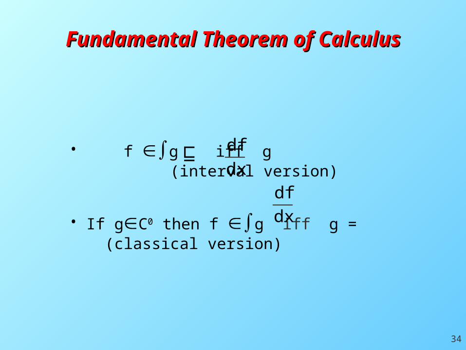
• f g iff g (interval version)
• If gC0 then f g iff g = (classical version)
Fundamental Theorem of CalculusFundamental Theorem of Calculus
dx
df
⊑dx
df

35
• We can approximate ( h, h′ ) in ([0,1] IR)2
i.e. ( f, g) ⊑ ( h ,h′ ) with f ⊑ h and g ⊑h′
• If h C1[0,1] , then
( h , h′ ) ([0,1] IR) ([0,1] IR)
Idea of Domain for Idea of Domain for CC11 Functions Functions
• What pairs ( f, g) ([0,1] IR)2 approximate a differentiable function?

36
• Proposition (f,g) Cons iff there is a continuous h: dom(g) R with f h ⊑ and g .⊑
Function and Derivative ConsistencyFunction and Derivative Consistency
• Define the consistency relation:Cons ([0,1] IR) ([0,1] IR) with(f,g) Cons if (f) ( g)
• In fact, if (f,g) Cons, there are least and greatest functions h with the above properties in each connected component of dom(g) which intersects dom(f) .
dx
dh
37
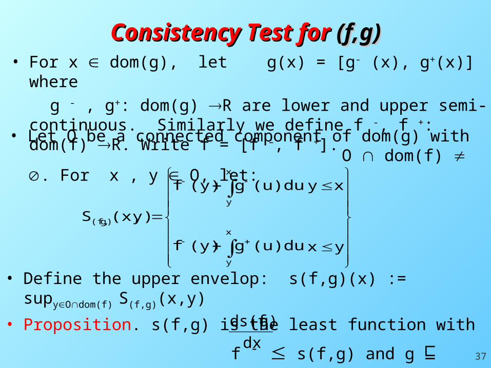
• For x dom(g), let g(x) = [g- (x), g+(x)] where
g - , g+: dom(g) R are lower and upper semi-continuous. Similarly we define f -, f +: dom(f) R. Write f = [f –, f +].
• Let O be a connected component of dom(g) with O dom(f) . For x , y O, let:
Consistency Test for Consistency Test for (f,g)(f,g)
yx(u)dug(y)f
xy(u)dug(y)f
y)(x,Sx
y
x
y
g)(f,
• Define the upper envelop: s(f,g)(x) := supyOdom(f) S(f,g)(x,y)
• Proposition. s(f,g) is the least function with
f - s(f,g) and g ⊑ dx
g)ds(f,

38
• The lower envelop: t(f,g)(x) := inf yOdom(f) (f +(y) + T (f,g) (x,y))
• Proposition. t(f,g) is the greatest function with
t(f,g) f+ and g ⊑
• Theorem. (f, g) Con iff for all component O of dom(g) with O dom(f) and all x O. s (f, g) (x) t (f, g) (x).
yx(u)dug(y)f
xy(u)dug(y)f
y)(x,Tx
y
x
y
g)(f,
Similarly, let:
dx
g)dt(f,

39
Approximating function: f = ⊔i ai↘bi
• (⊔i ai↘bi, ⊔j cj↘dj) Cons is a finitary property:
Consistency for basis elementsConsistency for basis elements
s(f,g) = least function
t(f,g)= greatest function
Approximating derivative: g = ⊔j cj↘dj

40
f
1
1
Function and Derivative Function and Derivative Information Information
g
1
2

41
f
1
1
Least and greatest functionsLeast and greatest functions
g
1
2

42
Decidability of consistencyDecidability of consistency
• Hence s(f,g) is the max of k+2 rational linear maps.
• Similarly for t(f,g)(x).
• Thus, s(f,g) t(f,g) is decidable.
• Theorem. Consistency is decidable.
myy
• Proposition. For x O, we have: s(f,g)(x) = max {f –(x) , limsup f –(y) + S(f,g) (x , y) | ym O dom(f) }
• For (f, g) = (⊔1in ai↘bi , ⊔1jm cj↘dj),
the rational end–points of ai and cj induce a partition y0 < y1 < y2 < … < yk of the connected component O of dom(g).

43
• Lemma. Cons ([0,1] IR)2 is Scott closed.
• Theorem.D1 [0,1]:= { (f,g) ([0,1]IR)2 | (f,g) Cons} is a continuous Scott domain, which can be given an effective structure.
The Domain of The Domain of CC11 FunctionsFunctions
• Theorem. : C0[0,1] D1 [0,1]
f (f , ) is topological embedding, giving a
computational model for continuous functions and their differential properties. It restricts to give an embedding of C1[0,1].
dx
df

44
Functions of several varibalesFunctions of several varibales
• (IR)1× n row n-vectors with entries in IR
• For dcpo A, let
(An)s = smash product of n copies of A:
x(An)s if x=(x1,…..xn) with xi non-bottomor x=bottom
• We work with (IR1× n)s

45
Definition of Interval Lipschitz constantDefinition of Interval Lipschitz constant
• f ([0,1]n IR) has an interval Lipschitz constantb (IR1xn)s in a I[0,1]n if x, y ao,
b(x – y) ⊑ f(x) – f(y).
• Proposition. If f(a,b), then f(x) Maximal (IR) for x ao and
for all x,y ao. |f(x)-f(y)| k ||x-y|| with k=max i (|bi+|, |bi
-|)
• The tie of a with b, is
(a,b) := { f | x,y ao. b(x – y) ⊑ f(x) – f(y)}
46
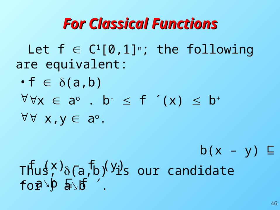
Let f C1[0,1]n; the following are equivalent:
• f (a,b)x ao . b- f ´(x) b+
x,y ao. b(x – y) ⊑ f (x) – f (y)
• a↘b ⊑ f ′
For Classical FunctionsFor Classical Functions
Thus, (a,b) is our candidate for a↘b .

47
Set of primitive mapsSet of primitive maps
: ([0,1]n IR) (P([0,1]n (IR1xn)s), ) ( P the power set constructor)
a↘b := (a,b)
supi I ai ↘ bi := iI (ai,bi)
is well-defined and Scott continuous. g can be the empty set for 2 n
Eg. g=(g1,g2), with g1(x , y)= y , g2(x, ,y)=0

48
The DerivativeThe Derivative
• Definition. Given f : [0,1]n IR the derivative of f is:
: [0,1]n (IR1xn)s
=sup {a↘b | f (a,b) }dx
dfdx
df
• Theorem. (Compare with the classical case.)
• is well–defined & Scott continuous.dx
df
'f Idx
If d
dx
df• If f C1[0,1], then
• f (a,b) iff a↘b ⊑

49
• f g iff g ⊑ (interval version)
• If gC0 then f g iff g = (classical version)
Fundamental Theorem of CalculusFundamental Theorem of Calculus
dx
df
dx
df

50
Relation with Clarke’s gradientRelation with Clarke’s gradient• For a locally Lipschitz f : [0,1]n IR
• ∂ f (x)=convex{ lim mf ´(xm) | x mx}
• It is a non-empty compact convex subset of Rn
• Theorem:
• For locally Lipschitz f : [0,1]n IR, the following holds:
• The domain-theoretic derivative at x , i.e. is the smallest
n-dimensional rectangle with sides parallel to the coordinate planes that contains ∂ f (x)
• In dimension one the two coincide.
dx
df

51
• If h C1[0,1]n , then
( h , h′ ) ([0,1]n IR) ([0,1]n IR)ns
Idea of Domain for Idea of Domain for CC11 Functions Functions
• What pairs ( f, g) ([0,1]n IR) ([0,1]n IR)ns
approximate a differentiable function?
• We can approximate ( h, h´ ) in ([0,1]n IR) ([0,1]n IR)n
s
i.e. ( f, g) ⊑ ( h ,h´ ) with f ⊑ h and g ⊑h´

52
Function and Derivative ConsistencyFunction and Derivative Consistency
• Define the consistency relation:Cons ([0,1]n IR) ([0,1]n IR)n
s with(f,g) Cons if (f) ( g)
• In fact, if (f,g) Cons, there are least and greatest functions h with the above properties in each connected component of dom(g) which intersects dom(f) .
• Proposition (f,g) Cons iff there is a continuous h: dom(g) R with f h ⊑ and g .⊑ dx
dh

53
Basis elementsBasis elements
• Definition. g:[0,1]n (IRn)s the domain of g is dom(g) = {x | g(x) non-bottom}
• Basis element: (f, g1,g2,….,gn) ([0,1]n IR) ([0,1]n IR)ns
• Each f, gi :[0,1]n IR is a rational step function. • Recall: the intersection of a closed and an open set is a crescent.• dom(g) is partitioned by disjoint crescents in each of which g is a constant
rational interval. .
[-2,2]
[-2,2]
[-3,3][-1,1]
Eg. For n=2:
A step function gi with four single step functions with two horizontal and two vertical rectangles as their domains and a hole inside, and with eight vertices.

54
Corners and their coaxial pointsCorners and their coaxial points
[-2,2]
[-2,2]
[-3,3][-1,1]
• Step function
• corners
• their coaxial points• vertices=corners coaxial points

55
Decidability of ConsistencyDecidability of Consistency
• (f,g) Cons if (f) ( g) • First we check if g is integrable, i.e. if g • In classical calculus, g:[0,1]n Rn will be integrable
by Green’s theorem iff for any piecewise smooth closed non-intersecting path
• p:[0,1] [0,1]n with p(0)=p(1)
0dt (t)p'g(p(t))1
0
• We generalize this to the type g:[0,1]n (IRn)s
56
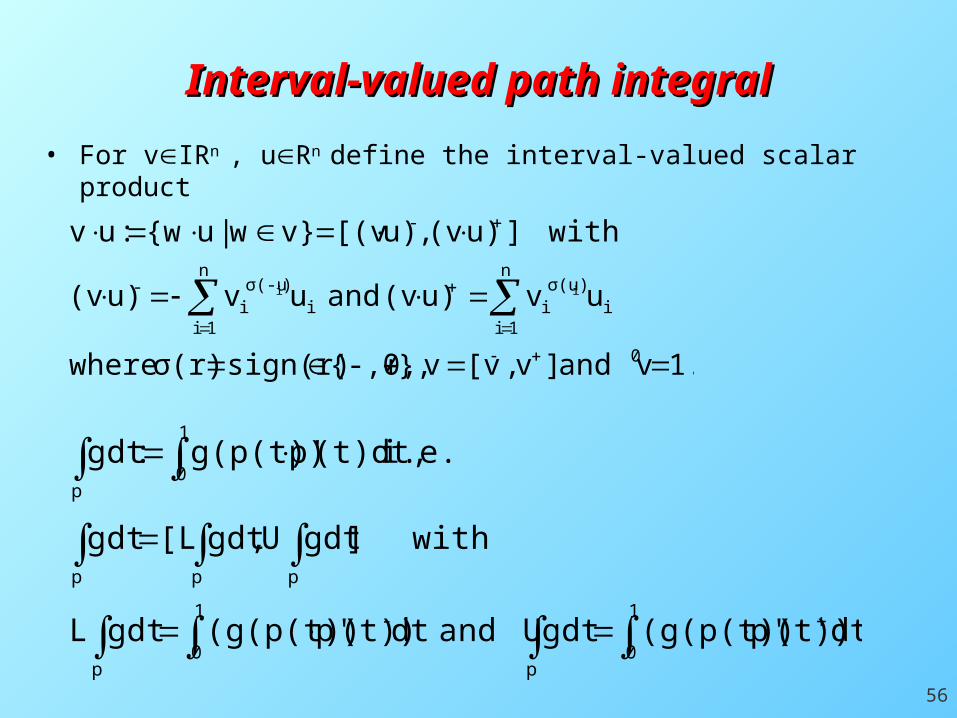
Interval-valued path integralInterval-valued path integral
• For vIRn , uRn define the interval-valued scalar product
1. vand ]v,[vv},{-,0, sign(r)σ(r) where
uvu)(v and uvu)(v
with]u)(v,u)[(vv}w|u{w:uv
0
n
1ii
)σ(ui
n
1ii
)σ(-ui
-
-
ii
dt(t))p' (g(p(t))gdt Uanddt (t))p' (g(p(t))gdtL
with]gdtU,gdt[Lgdt
i.e. (t)dt,p'g(p(t)):gdt
1
0p
-1
0p
ppp
1
0p

57
Generalized Green’s TheoremGeneralized Green’s Theorem
• Theorem. g iff for all piecewise smooth non-intersecting path p:[0,1] dom(g) with p(0)=p(1), we have zero-containment:
1
0(t)dtp'g(p(t))0
• For step functions, we can and will replace “smooth” with “linear”.
• Then, the lower and upper path integrals will depend piecewise linearly on the coordinates of nodes the path, so their extreme values will be reached when these nodes are at the corners of dom(g) or their coaxial points.
• Since there are finitely many of these extreme paths, zero containment can be decided in finite time for all paths.

58
Minimal surface for g Minimal surface for g
• Step function g:[0,1]n (IRn)s with g . Let O be a component of dom(g) . Let x,ycl(O).
• Consider the following supremum over all piecewise linear paths p in cl(O) with p(0 )= y and p(1)= x.
1
0pg (t)dt}p'g(p(t)){Lsupy)(x,V
• The above supremum is attanied.
• For fixed y, the map Vg (. ,y): cl(O) R is a rational piecewise linear function.
• It is the least continuous function or surface with:
• Vg (y ,y)=0 and g ⊑ dx
)(.,dVg y

59
Maximal surface for gMaximal surface for g
• Step function g:[0,1]n (IRn)s . Let O be a component of dom(g) . Let x,ycl(O).
• The following infimum is attained over all piecewise linear paths p in cl(O) with p(0 )= y and p(1)= x.
1
0pg (t)dt}p'g(p(t)){Uinfy)(x,W
• For fixed y, the map Wg (. ,y): cl(O) R is a rational piecewise linear function.
• It is the greatest continuous function or surface with:
• Wg (y ,y)=0 and g ⊑ dx
)(.,dWg y

60
Minimal surface for (f,g)Minimal surface for (f,g)
• (f,g)([0,1]n IR) ([0,1]n IR)ns rational step function
• Assume we have determined that g • Put
and (y)finflimy)(x,Vy)(x,S gg)(f,
dom(g)in x of component theOwith
}O y |y)(x,{S supg)(x)s(f,
x
xg)(f,
• Proposition.
dx
g)ds(f,
Theorem. s(f,g): dom(g) R is the least continuous function with
f - s(f,g) and g ⊑
)}O vertices(y |y)(x,{Smax g)(x)s(f, xg)(f,

61
Maximal surface for (f,g)Maximal surface for (f,g)
and (y)fsuplimy)(x,Wy)(x,T gg)(f,
}O y |y)(x,{T infg)(x)t(f, xg)(f,
dx
g)dt(f,Theorem. t(f,g): dom(g) R is the least continuous function with
t(f,g) f + and g ⊑
)}O vertices(y |y)(x,{Tmin g)(x) t(f,:have We xg)(f,
Theorem. Consistency is decidable.
Proof: In s(f,g)t(f,g) we compare two rational piecewise-linear surfaces, which is decidable.

62
• Lemma. Cons ([0,1]n IR) ([0,1]n IR)ns is Scott closed.
• Theorem.D1 [0,1]n:= { (f,g) | (f,g) Cons} is a continuous Scott domain that can be given an effective structure.
The Domain of The Domain of CC11 FunctionsFunctions
• Theorem. : C0[0,1]n D1 [0,1]n
f (f , ) is topological embedding, and so is its
restriction to C1[0,1]n , giving a computational model for continuous functions and their differential properties.
dx
df

63
ExampleExample
1
f
g
1
1
1
v
v is approximated by a sequence of step functions, v0, v1, …
v = ⊔i vi
We solve: = v(t,x), x(t0) =x0
for t [0,1] with
v(t,x) = t and t0=1/2, x0=9/8.
dt
dx
a3
b3
a2
b2
a1
b1
v3
v2
v1
The initial condition is approximated by rectangles aibi:
{(1/2,9/8)} = ⊔i aibi,
t
t
.

64
SolutionSolution
1
f
g
1
1
1
At stage n we find un
- and un +
.

65
SolutionSolution
1
f
g
1
1
1 .
At stage n we find un
- and un +

66
SolutionSolution
1
f
g
1
1
1 un - and un
+ tend to
the exact solution:f: t t2/2 + 1
.
At stage n we find un
- and un +

67
Computing with polynomial step Computing with polynomial step functionsfunctions

68
Some Open ProblemsSome Open Problems
• Topologically, what sort of a set is (a,b) ?• Topologically, what sort of a set is C0 in the set of maximal
elements of D0=[0,1]IR? Similarly, for C1 as a subset of maximal elements of D1.
• For a domain of twice differentiable functions, is consistency decidable? (It is true for n=1.)
• Decidability of consistency for 3rd and higher derivatives (not known even for n=1).
• Construct a domain for analytic functions.• For solving PDE’s, obtain a domain-theoretic version of the
finite difference and finite element methods.

Part III: Part III: A Domain-Theoretic Model of A Domain-Theoretic Model of
GeometryGeometry
• To develop a model for Computational Geometry and Solid Modelling, so that:
• the model is mathematically sound, realistic;
• the basic building blocks are computable;
• it bridges theory and practice.

70
Why do we need a data type for Why do we need a data type for solids?solids?
Answer: To develop robust algorithms!
Lack of a proper data type and use of real RAM in which comparison of real numbers is decidable give unreliable programs in practice!

71
The Intersection of two linesThe Intersection of two lines
With floating point arithmetic, find the point P of the intersection L1 L2. Then: min_dist(P, L1) > 0, min_dist(P, L2) > 0.
1L
2LP

72
The Convex Hull AlgorithmThe Convex Hull Algorithm
A, B & C nearly collinear A
B
C
With floating point we can get:
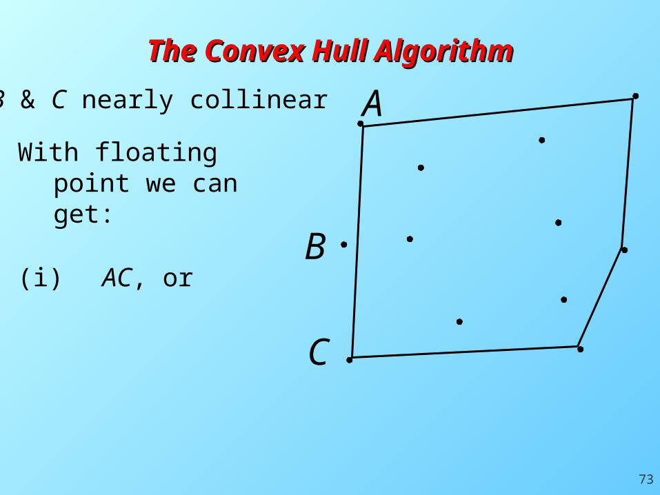
73
A, B & C nearly collinear
The Convex Hull AlgorithmThe Convex Hull Algorithm
A
B
C
With floating point we can get:
(i) AC, or

74
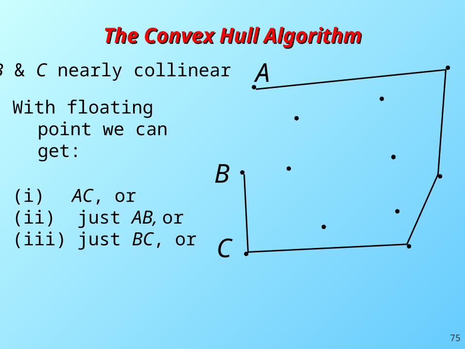
A, B & C nearly collinear
The Convex Hull AlgorithmThe Convex Hull Algorithm
A
B
C
With floating point we can get:
(i) AC, or(ii) just AB, or
75
A, B & C nearly collinear
The Convex Hull AlgorithmThe Convex Hull Algorithm
A
B
C
With floating point we can get:
(i) AC, or(ii) just AB, or(iii) just BC, or

76
A, B & C nearly collinear
With floating point we can get:
(i) AC, or(ii) just AB, or(iii) just BC, or(iv) none of them.
The quest for robust algorithms is the most fundamental unresolved problem in solid modelling and computational geometry.
The Convex Hull AlgorithmThe Convex Hull Algorithm
A
B
C

77
• Subset A X topological space.
Membership predicate A : X {tt, ff }
is continuous iff A is both open and closed.
Axff
Axttx
A Fundamental Problem in Topology A Fundamental Problem in Topology and Geometryand Geometry
• In particular, for A Rn, A , A Rn
A : Rn {tt, ff } is not continuous.
• Most engineering is done, however, in Rn.

78
• There is discontinuity at the boundary of the set.
x
Non-computability of the Non-computability of the Membership PredicateMembership Predicate
• This predicate is not computable:
x If x is on the boundary, we cannot in general determine if it is in or out at any finite stage of computation.
FalseTrue

79
Non-computable Operations in Non-computable Operations in Classical CG & SMClassical CG & SM
• A: Rn {tt, ff} not continuous means it is not computable, even for simple objects like A=[0,1]n.
• x A is not decidable even for simple objects: for A = [0,) R, we just have the undecidability of x 0.
• The Boolean operation is not continuous, hence noncomputable, wrt the natural notion of topology on subsets: : C(Rn) C(Rn) C(Rn), where C(Rn) is compact subsets with the Hausdorff metric.

80
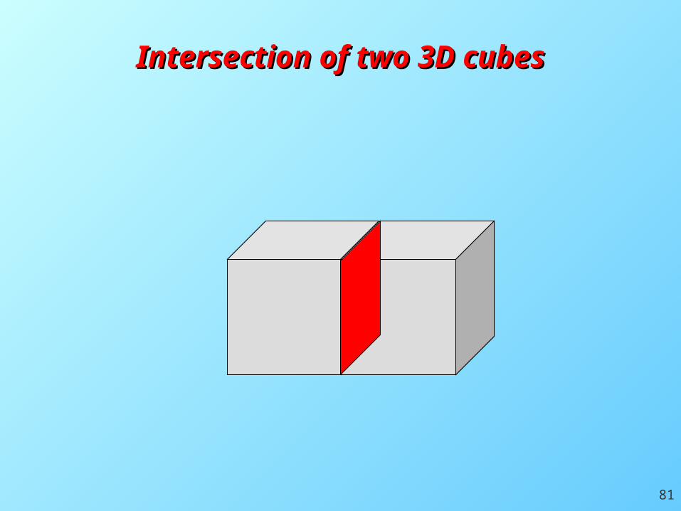
Intersection of two 3D cubesIntersection of two 3D cubes
81
Intersection of two 3D cubesIntersection of two 3D cubes
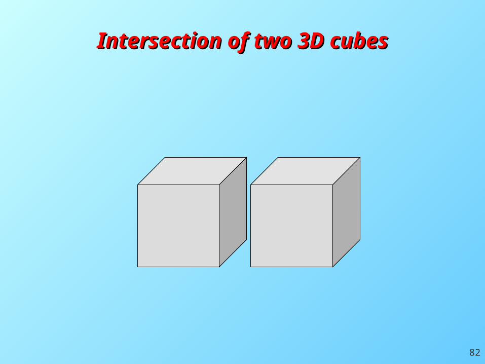
82
Intersection of two 3D cubesIntersection of two 3D cubes

83
This is Really Ironical!This is Really Ironical!
• Topology and geometry have been developed to study continuous functions and transformations on spaces.
• The membership predicate and the binary operation for are the fundamental building blocks of topology and geometry.
• Yet, these fundamental functions are not continuous in classical topology and geometry.
84
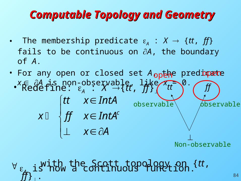
Computable Topology and GeometryComputable Topology and Geometry
• The membership predicate A : X {tt, ff} fails to be continuous on A, the boundary of A.
• For any open or closed set A, the predicate x A is non-observable, like x = 0.
• Redefine: A : X {tt, ff}
with the Scott topology on {tt, ff}.
Ax
IntAxff
IntAxtt
x c
tt ff
open
open
observable observable
Non-observable
A is now a continuous function.

85
Elements of a Computable Elements of a Computable Topology/GeometryTopology/Geometry
• Note that A=B iff int A=int B & int Ac=int Bc,
i.e. sets with the same interior and exterior have the same membership predicate.
• We now change our view: In analogy with classical set theory where every set is completely determined by its membership predicate, we define a (partial) solid object to be given by any continuous map:
f : X { tt, ff }
• Then:f –1{tt} is open; it’s called the interior of the object. f –1{ff} is open; it’s called the exterior of the object.
86
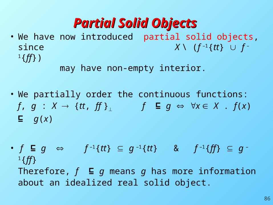
Partial Solid ObjectsPartial Solid Objects • We have now introduced partial solid objects, since
X \ (f –1{tt} f –1{ff}) may have non-empty interior.
• We partially order the continuous functions:f, g : X {tt, ff } f ⊑ g x X . f(x) ⊑ g(x)
• f ⊑ g f –1{tt} g –1{tt} & f –1{ff} g –1{ff}Therefore, f ⊑ g means g has more information about an idealized real solid object.

87
The Geometric (Solid) Domain of The Geometric (Solid) Domain of XX• The geometric (solid) domain S (X) of X is the poset
(X {tt, ff }, ⊑ )
• S(X) is isomorphic to the poset SO(X) of pairs of disjoint open sets
(O1,O2) ordered componentwise by inclusion:
21
212
1
11
),(
otherwise
}){},{(
)( )(
OO
OOOxff
Oxtt
x
fffttff
XSXS O

88
• Theorem For a second countable locally compact Hausdorff space X (e.g. Rn), S(X) is bounded complete and –continuous (i.e. a continuous Scott domain) with (U1, U2) << (V1, V2) iff the closures of U1 and U2 are
compact subsets of V1 and V2 respectively.
• Theorem If X is Hausdorff, then: (O1, O2) Maximal (S X, ⊑) iff
O1= int O2c & O2= int O1
c.
This is a regular solid object: O1=int O1 & O2=int O2
Properties of the Geometric (Solid) Properties of the Geometric (Solid) DomainDomain
• Definition (O1, O2) , O1 ≠ ∅ ≠ O2 , is a classical object if O1 ∪ O2 = X.

89
ExamplesExamples• A = {xR2 |x| ≤ 1} ⃒� [1, 2]
represented in the model byArep = (int A, int Ac) =
( {x | ⃒� x| < 1}, R2 \ A )is a classical (but non-regular) solid object.
• B = {xR2 |x| ≤ 1} ⃒�represented by Brep=
({x | ⃒� x| < 1} , {x | ⃒� x| > 1}) Maximal (SR2, ⊑)is a regular solid object with Arep ⊑ Brep.

90
Boolean operations and Boolean operations and predicatespredicates
Theorem All these operations are Scott continuous and preserve classical solid objects.
),()),( , ),((
:
22112121 BABABBAA
SXSXSX
),(),(
:
1221 OOOO
SXSX
),()),( , ),((
:
22112121 BABABBAA
SXSXSX

91
Subset InclusionSubset Inclusion
otherwise.
)),(),,((
},{:
21
12
2121 BAff
XBAtt
BBAA
ffttSXXSb
• Subset inclusion is Scott continuous.
.)},{( compact} |),{( 221 cb ASXAAXS• Let
92
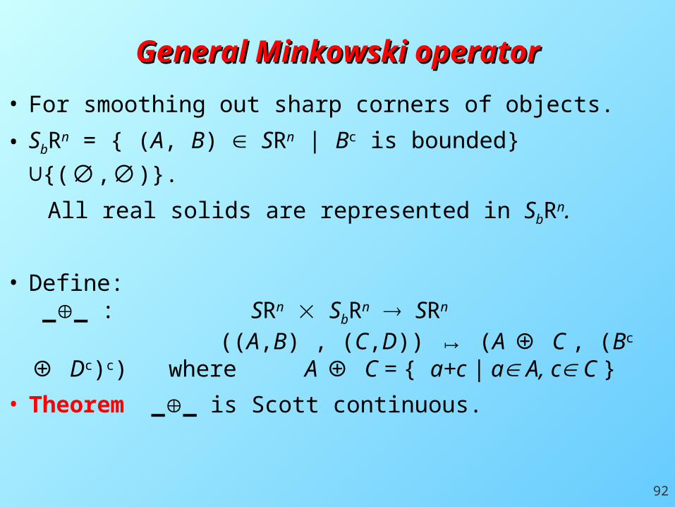
General Minkowski operatorGeneral Minkowski operator
• For smoothing out sharp corners of objects.
• SbRn = { (A, B) SRn | Bc is bounded} {( , )}.∪ ∅ ∅
All real solids are represented in SbRn.
• Define: __ : SRn SbRn SRn
((A,B) , (C,D)) (↦ A ⊕ C , (Bc ⊕ Dc)c) where A ⊕ C = { a+c | a A, c C }
• Theorem __ is Scott continuous.

93
• (A, B) is a computable partial solid object if there exists a total recursive function ß:NN such that : ( K ß(n) ) n 0 is an increasing chain with:
An effectively given solid domainAn effectively given solid domain
• The geometric domain SX can be given effective structure for any locally compact second countable Hausdorff space, e.g. Rn, Sn, Tn, [0,1]n.
• Consider X=Rn. The set of pairs of disjoint open rational bounded polyhedra of the form K = (L1 , L2) , with L1 L2 = , gives a basis for SX.
• Let Kn= (π1 ( K n ) , π2 ( K n) ) be an enumeration of this basis.
(A , B) = supnK ß(n) =( ∪n π1 ( K ß(n) ) , ∪n π2 ( K ß(n) ) )

94
Computing a Solid ObjectComputing a Solid Object
• In this model, a solid object is represented by its interior and exterior.
• The interior and the exterior
are approximated by two
nested sequence of rational polyhedra.

95
Computable Operations on the Computable Operations on the Solid DomainSolid Domain
• F: (SX)n SX or F: (SX)n { tt, ff }
is computable if it takes computable sequences of partial solid objects to computable sequences.
• Theorem All the basic Boolean operations and predicates are computable wrt any effective enumeration of either the partial rational polyhedra or the partial dyadic voxel sets.

96
Quantative Measure of ConvergenceQuantative Measure of Convergence
• In our present model for computable solids, we require a quantitative measure for the convergence of the basis elements to a computable solid.
• We will enrich the notion of domain-theoretic computability in two different ways to include a quantitative measure of convergence.

97
• We strengthen the notion of a computable solid by using the Hausdorff distance d between compact sets in Rn.
• d(C,D) = min{ r>0 | C Dr & D Cr } where Dr = { x | y D. |x-y| r }
• (A , B) S [–k, k]n is Hausdorff computable
if there exists an effective chain Kß(n) of basis elements with ß :NN a total recursive function such that:
(A , B) = ( ∪n π1 ( K ß(n) ) , ∪n π2 ( K ß(n) ) )
with
d (π1 ( K ß(n) ) , A ) < 1/2n , d (π2 ( K ß(n) ) , B) < 1/2n
Hausdorff ComputabilityHausdorff Computability

98
Hausdorff computabilityHausdorff computability
• Two solid objects which have a small Hausdorff distance from each other are visually close.
• The Hausdorff distance gives a natural quantitative measure for approximation of solid objects.
• However, the intersection or union of two Hausdorff computable solid objects may fail to be Hausdorff computable.
• Examples of such failure are nontrivial to construct.

99
Boolean Intersection is not Hausdorff Boolean Intersection is not Hausdorff computablecomputable
nQ
0r 1r 1nr nr r
21
121n
n21
0
.computableleft
rational,
nn
nn
rrr
However:
Q([0,1] {0})= [r,1] {0} R2
is not Hausdorffcomputable.
is Hausdorff computable.
)0,0( )0,1(
)1,1()1,0(

100
Lebesgue ComputabilityLebesgue Computability
• (A , B) S [–k, k]d is Lebesgue computable iff there
exists an effective chain Kß(n) of basis elements with ß
:NN a total recursive function such that:
(A , B) = ( ∪n π1 ( K ß(n) ) , ∪n π2 ( K ß(n) ) )
µ(A) - µ(π1 ( K ß(n) ) ) < 1/2 n & µ(B) - µ(π2 ( K ß(n) ) ) < 1/2
n
• A computable function is Lebesgue computable if it
preserves Lebesgue computable sequences.
• Theorem Boolean operations are Lebesgue computable.

101
• Hausdorff computable ⇏ Lebesgue computableComplement of a Cantor set with Lebesgue measure 1– r with r =lim rn: left computable but non-computable real.
, ,0m
n
0m1 rsrsrrs mnmnnn
0 1
s0
• At stage n remove 2n open mid-intervals of length sn/2n.
• start with
• stage 1
• stage 2
21s
21s

102
Hausdorff and Lebesgue Hausdorff and Lebesgue computabilitycomputability
• Lebesgue computable ⇏ Hausdorff computable
Let 0 < rn Q with rn ↗ r, left computable, non-computable 0 < r < 1.
0r nr r0 1
• Then [r,1] {0} R2 is Lebesgue computable but not Hausdorff computable.

103
• Hausdorff computable ⇏ Lebesgue computable
• Lebesgue computable ⇏ Hausdorff computable
• Theorem: A regular solid object is computable iff it is Hausdorff computable.
• However: A computable regular solid object may not be Lebesgue computable.
Hausdorff and Lebesgue Computable Hausdorff and Lebesgue Computable ObjectsObjects

104
Summary Summary
Our model satisfies: A well-defined notion of computability Reflects the observable properties of geometric objects Is closed under basic operations Captures regular and non-regular sets Supports a methodology for designing robust algorithms

105
Data-types for Computational Data-types for Computational Geometry and Systems of Linear Geometry and Systems of Linear
EquationsEquations
• The Convex Hull
• Voronoi Diagram or the Post Office problem
• Delaunay Triangulation
• The Partial Circle through three partial points
106
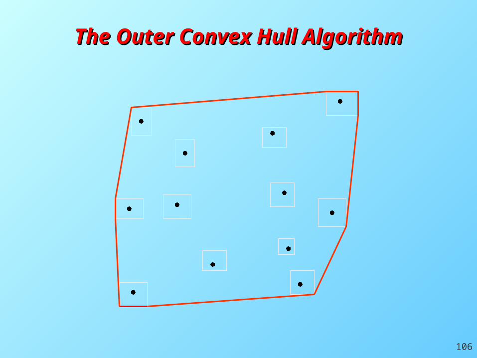
The Outer Convex Hull AlgorithmThe Outer Convex Hull Algorithm

107
The Inner Convex Hull AlgorithmThe Inner Convex Hull AlgorithmTop right cornersTop left corners
bottom right cornersbottom left corners

108
The Convex Hull AlgorithmThe Convex Hull Algorithm

109
The Convex Hull AlgorithmThe Convex Hull Algorithm
110
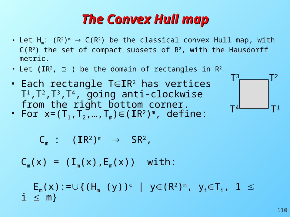
• Let Hm: (R2)m C(R2) be the classical convex Hull map, with C(R2) the set of compact subsets of R2, with the Hausdorff metric.
• Let (IR2, ) be the domain of rectangles in R2.
The Convex Hull mapThe Convex Hull map
• For x=(T1,T2,…,Tm)(IR2)m, define:
Cm : (IR2)m SR2,
Cm(x) = (Im(x),Em(x)) with:
Em(x):={(Hm (y))c | y(R2)m, yiTi, 1 i m}
Im(x):= {(Hm (y))0 | y(R2)m, yiTi, 1 i m}
T1
T2T3
T4
• Each rectangle TIR2 has vertices T1,T2,T3,T4, going anti-clockwise from the right bottom corner.

111
The Convex Hull is Computable!The Convex Hull is Computable!
• Proposition: Em(x)=(H4m((Ti1,Ti
2,Ti3,Ti
4))1im)c
Im(x)=Int({Hm((Tin))1im) | n=1,2,3,4}).
• Theorem: The map Cm : (IR2)m SR2 is Scott continuous, Hausdorff and Lebesgue computable.
• Complexity:
1. Em(x) is O(m log m).
2. Im(x) is also O(m log m).
We have precisely the complexity of the classical convex hull algorithm in R2 and R3.

112
Voronoi DiagramsVoronoi Diagrams• We are given a finite number of points in the plane.
• Divide the plane into components closest to these points.
• The problem is equivalent to the Delaunay triangulation of the points:
(1) Triangulate the set of given points so that the interior of the circumference circles do not contain any of the given points. (2) Draw the perpendicular bisectors of
the edges of the triangles.

113
• Recall that the Voronoi diagram is dual to the Delaunay triangulation: Given a finite number of points of the plane find the triples of points so that the interior of the circle through
any triple does not contain any other points. . .
.. .
.
Voronoi Diagram & Partial CirclesVoronoi Diagram & Partial Circles
• The centre of the circle through the three vertices of a triangle is the intersection of the perpendicular bisectors of the three edges of the triangle.
• The partial circle of three partial points in the plane is obtained by considering the Partial Perpendicular Bisector of two partial points in the plane.

114
Partial Perpendicular Bisector of Two Partial Perpendicular Bisector of Two Partial PointsPartial Points

115
PPBs for Three Partial PointsPPBs for Three Partial Points
Partial Centre

116
Partial CirclesPartial Circles
The Interior is the intersection of the interiors of the three blue circles.
The exterior is the union of the exteriors of the three red circles.
Each partial circle is defined by its interior and exterior. The exterior (interior) consists of all those points of the plane which are outside (inside) all circles passing through any three points in the three rectangles.

117
Partial CirclesPartial CirclesWith more exact partial points, the boundaries of the interior and exterior of the partial circle get closer to each other.

118
Partial CirclesPartial Circles
• In the limit, the area between the interior and exterior of the partial circle, and the Hausdorff distance between their boundaries, tends to zero.
• We get a Scott continuous map C : (IR2)3SR2
• We obtain a robust Voronoi algorithm.

119
Part IVPart IVInverse and Implicit Function TheoremsInverse and Implicit Function Theorems
Domain of ManifoldsDomain of Manifolds
• The mains tool in multi-variable calculus.• In CAD curves and surfaces are built from the implicit
function theorem, f(x,y,z) = 0 for a C1 map f: R3 R
• A domain-theoretic framework can be the basis of a robust CAD.
• Implicit function theorem follows from the inverse function theorem, both
classically and domain-theoretically.

120
Calculus of operations in DCalculus of operations in D11
• For a vector function f = (fi)i := (fi)1≤i≤n we write fD1 ([0,1]n Rn) if fiD1 ([0,1]n R) for 1 ≤i ≤ n
• The following operations are well-defined and Scott continuous:
• - - : D1 ([0,1]n IRn)× D1 ([0,1]n IRn) D1 ([0,1]n IRn)
( f , g ) f g
with (f g)i = ( fi0 gi0 , fi1 gi1 ,…….., fin gin )
• - ◦ - : D1 (Rn IRn)× D1 ([0,1]n IRn) D1 ([0,1]n IRn)
( f , g ) f◦g
)g)(gIf,.....,g)(gIf,)(g(Ifg)(f knjj0
n
1k ikk1jj0
n
1k ikjj0i0i
• This extends the higher dimensional chain rule.

121
Inverse Constructor (function part)Inverse Constructor (function part)
• Idea: First find the inverse of a map which differs from the identity map by a contraction
• Let A=[-a,a]n and B=[-ca,ca]n for a> 0 and 0< c ≤1/2
• V: (A→IB)×(B→IB)→(B→IB)
• (f,g) → - If ◦ (id+g) , where id is the identity map.
• Theorem. Suppose f:[-a,a]n→Rn has Lipschitz constant nc<1 wrt the max norm and f(0)=0. Then
• V(f , .): (B→IB)→(B→IB) has a unique fixed point g satisfying g - = g+ and g(0)=0
• id+f : [-a,a]n→Rn has inverse id+g
In fact: g = - f ◦ (id+g) implies (id +f)◦(id+g) = id+ g – g = id
122
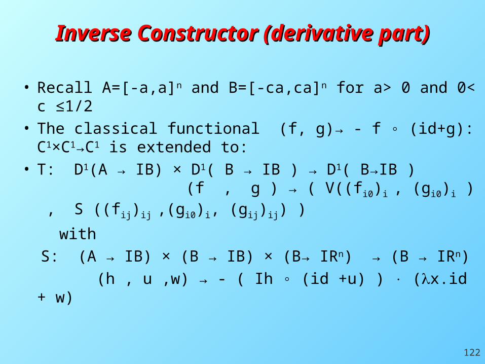
Inverse Constructor (derivative part)Inverse Constructor (derivative part)
• Recall A=[-a,a]n and B=[-ca,ca]n for a> 0 and 0< c ≤1/2• The classical functional (f, g)→ - f ◦ (id+g): C1×C1→C1
is extended to:• T: D1(A → IB) × D1( B → IB ) → D1( B→IB )
(f , g ) → ( V((fi0)i , (gi0)i ) , S ((fij)ij ,(gi0)i, (gij)ij) )
with
S: (A → IB) × (B → IB) × (B→ IRn) → (B → IRn)
(h , u ,w) → - ( Ih ◦ (id +u) ) (x.id + w)

123
Invesre Constructor (derivative part)Invesre Constructor (derivative part)
• Suppose f:[-a,a]n→Rn has Lipschitz constant nc < 1 wrt the max norm and f(0)=0. Then the functional
IB)(BDIB)(BD :) - ),dx
dfT((f, 11
has a unique fixed point ((gi0)i,(gij)ij) where (gi0)i is the unique fixed point of V(f,-) and (gij)ij is the unique fixed point of
IB)(BIB)(B :) - ,)(g,dx
dfS( ii0
• If f '(x) exists for some x[-a,a]n, so does (gi0)i '(x) and we have:
(gi0)i ' (x) = (gij)ij (x)

124
Mean DifferentialMean Differential
• Lemma u: [-a,a]n → Rn has Lipschitz constant nc<1 wrt the max norm iff uiδ([-a,a]n ,[-c,c]) for 1 ≤i ≤ n
]))(xdx
du())(x
dx
du[(
2
1M ij0ij0ij
• Definition. Given u:[-1,1]nRn , the mean differential at x0 :[-1,1]n is the linear map represented by the matrix M with
• Proposition. Suppose the mean differential M of u:[-1,1]n Rn at 0 is invertible with k:=|| M-1 - id || < 1/n. Then, for any c with k< c <1, there exists a>0 such that the map f=M-1 u- id: [-a,a]n → Rn satisfies fiδ([-a,a]n ,[-c,c]) for 1 ≤i ≤ n; thus the map f has Lipschitz constant nc<1 wrt the max norm
(0)dx
du

125
Inverse Function theoremInverse Function theorem
• Theorem. Let u:[-1,1]n Rn and suppose the mean differential
M of u at 0 is invertible with || M-1 - id || < 1/n. Then:(0)dx
du
• The map u has a Lipschitz inverse in a neighbourhood of 0 .
• Given an increasing sequence of linear step functions converging to u, we can effectively obtain an increasing sequence of linear step functions converging to u-1
• If furthermore u is C1 and given also an increasing sequence of linear step functions converging to u' we can also effectively obtain an increasing sequence of polynomial step functions converging to (u-1)'

126
Current and Further WorkCurrent and Further Work
• A domain (w-continuous dcpo)for Lipschitz manifolds with basisgiven by rational piecewise linearmanifold (i.e., polyhedra).
• Construct the kernel of a robust CAD, based on domain-theoretic approximations to curves and surfaces obtained by the implicit function theorem.