DOI:10.5545/sv-jme.2012.677 The Effect of Surface ... coating technology, tool geometry design, ... and selection of ... including pressure die casting tools, extrusion tools, forging

Strojniški vestnik - Journal of Mechanical Engineering 59(2013)2, 124-134 Received for review: 2012-06-26© 2013 Journal of Mechanical Engineering. All rights reserved. Received revised form: 2012-12-03DOI:10.5545/sv-jme.2012.677 Accepted for publication: 2013-01-14

*Corr. Author’s Address: National Formosa University, 64 Wunhua Road, Huwei, Yunlin 632, Taiwan, [email protected]

0 INTRODUCTION

Developments in machine tools tend towards high speed technology, including high-speed machining (HSM) and high-speed cutting (HSC), especially in high speed end milling applications [1] and [2]. High speed technology applications in machine tools are characterised by a high feeding speed, low axial and radial cutting depth, increased metal removal rate, simplified processing, and reduced costs. The thermal effect of workpieces is insignificant since cutting chips remove most of the heat induced by processing, and hence cutting oil is seldom used. This trend contributes to environmental protection efforts. Only a small amount of cutting fluid is available to lubricate green cutting. The primary deformation zone is significantly heated and bears the cutting force. Therefore, major green cutting methods include tool materials, coating technology, tool geometry design, chip control, coefficient of tool-face friction with the workpiece, and selection of cutting. Green cutting-related developments and applications depend on technological advances in machinery and cutting tools.

The grinding precision of cutting tools is determined by the surface roughness of the rake face and relief face, in which precision essentially affects the surface roughness of a workpiece and the tool life during high-speed milling. Generally, a cutting tool manufacturer evaluates the quality of grinding,

first, with respect to the surface finish of end-mill, and then with by the geometrical profile. The surface finish, which influences the abrasion of the end-mill, lubrication, accuracy, and tool life expectancy, depends on the surface roughness of the rake face and relief face.

As the most important and the final procedure in manufacturing, grinding of cutting edges is also critical in determining geometrical shapes, cutting performance, wear on the cutting edge, and tool life [3]. Shaji and Radhakrishnan [4] analysed the grinding parameters with respect to surface characteristics, e.g., wheel, workpiece, processing, and mechanical parameters. Yin et al. [5] examined ultraprecision grinding of cemented carbides from a microstructure perspective. Kwak [6] diagnosed errors in surface grinding processing by Taguchi and response surface methods. Nguyen et al. [7] simulated impact parameters of the precision grinding process.

Owing to its efficiency and systematic approach, the Taguchi method has been extensively adopted in parameter design and experimental planning [8]. Despite its application in optimizing process parameters [9] to [13], the Taguchi method is unsatisfactory for handling multiple performance characteristics. In this study we attempt to derive an efficient solution to overcome the above problem.

Grey relational analysis based on the Taguchi method can be adopted to elucidate the complex relationship among the designated performance

The Effect of Surface Roughness of End-Mills on Optimal Cutting Performance for High-Speed Machining

Chen, C.H. – Wang, Y.C. – Lee, B.Y.Chi-Hsiang Chen1,* – Yung-Cheng Wang2 – Bean-Yin Lee3

1Institute of Mechanical and Electro-Mechanical Engineering, National Formosa University, Taiwan 2Institute of Mechanical Engineering, National Yunlin University of Science & Technology, Taiwan

3Department of Mechanical and Computer-Aided Engineering, National Formosa University, Taiwan

In this study, the effect of surface roughness of end-mills on the cutting performance of high-speed machining has been investigated. A novel optimization design approach of the processing parameters for the high-speed cutting of the DIN 1.2344 tool steel has been also proposed. The characteristics indices of cutting performance selected for this investigation are tool life and metal removal rate. The processing parameters include the surface roughness of the relief face of an end-mill, cutting speed, feed per tooth, axial cutting depth, and radial cutting depth. The process is integrated using multiple performance indices. Consequently, the optimal combination of processing parameters is determined by performing grey relational analysis. The analysis results indicate that the effect of cutting speed and feed per tooth are significant for multiple performance characteristics. Additionally, the surface roughness of the relief face of an end-mill essentially affects the surface roughness of the processed workpiece. Due to a slight effect on the cutting performance characteristics of rough machining, a surface roughness of the relief face of 0.43±0.02 μm for grinding conditions can be used to improve tool grinding efficiency. Verification experiments revealed that the proposed optimization design approach to the processing parameters brings about improvements of 9.1 min in tool life, 1200 mm3/min in metal removal rate, 230616 mm3 in total metal removal volumes, and 0.044 μm in average surface roughness of the workpiece with high-speed cutting.Keywords: high-speed cutting, grey relational analysis, surface roughness, end-mill

Strojniški vestnik - Journal of Mechanical Engineering 59(2013)2, 124-134

125The Effect of Surface Roughness of End-Mills on Optimal Cutting Performance for High-Speed Machining

characteristics. Through this analysis, a grey relational grade is favorably defined as an indicator of the multiple performance characteristics for evaluation. Grey relational analysis is a highly effective means of analysing processes with multiple performance characteristics [14] to [18].

This paper is schemed as follows. In Section 1, we will describe the analysis method. Then, in Section 2, the importance of the surface roughness of the relief face in the workpiece will be investigated. In Section 3 the optimal experimental design and results will be summarized. Section 4 and 5 will describe, the result analyses, discussions and conclusions.. The end-mill with a the-lower-the-better condition can produce improved machining quality and tool life. Therefore, in this study, processing parameters are estimated by adding in the surface roughness of the relief face of an end-mill to the other other processing parameters, which include cutting speed, feed per tooth, axial cutting depth and radial cutting depth. Moreover, the characteristics of the cutting performance are the tool wear rate and the metal removal rate, which belong to the multiple performance characteristics. How to optimize the HSC process based on grey relational analysis and an analysis of cutting performance characteristics in end-milling for HSC are discussed in detail.

1 ANALYSIS METHODS

1.1 Signal-to-Noise Ratio

The Taguchi method is a simple and effective solution for parameter design and experimental planning [19]. In this method, the signal-to-noise (S/N) ratio is used to represent a performance characteristic in which the largest value of the S/N ratio is required. The three S/N ratios are the lower-the-better, the higher-the-better, and the nominal-the-better. The S/N ratio with a lower-the-better characteristic can be illustrated as follows:

ηij n ijj

ny= −

=∑10 1 2

1log . (1)

The S/N ratio with a higher-the-better characteristic can be expressed as follows:

ηij nijj

n

y= −

=

∑10 112

1log ,

where yij is the ith experiment at the jth test and n is the total number of the tests, in this study n = 2.

1.2 Grey Relational Analysis

Grey relational analysis initially generates data preprocessing to normalize the raw data. Here, the S/N ratio is linearly normalized in the range between 0 and 1, which is also called grey-relational generating [20]. The normalized S/N ratio xij for the ith performance characteristic in the jth experiment can be described as follows:

xijij j ij

j ij j ij=

−

−

η η

η η

minmax min

, (3)

where i = 1, …, m; j = 1, …, n. m denotes the number of experimental data items and n represents the number of parameters, with m = 18 and n = 2 in this study. Basically, the larger normalized S/N ratio corresponds to the better performance and the best-normalized S/N ratio is equal to unity.

In gray relational analysis, the evaluation of the relevancy between two systems or two sequences is defined as the gray relational grade. The local gray relation measurement refers to a situation in which only one sequence follows data preprocessing. The gray relation coefficient ζij for the ith performance characteristics in the jth experiment can be expressed as follows:

ζζ

ζij

i j i ij i j i ij

i ij i j i

x x x x

x x x x=

− + −

− + −

min min max max

max max

0 0

0 0iij

, (4)

where xi0 is the ideal sequence for the ith performance

characteristic; xij represents the comparability sequence; ζ refers to the distinguishing coefficient, which is defined in the range 0 ≤ ζ ≤ 1, in this study ζ = 0.5.

The grey relational grade is a weighting-sum of the grey relational coefficients. It is defined as follows:

γ β ζ βj k ijk

m

kk

m

m= =

= =∑ ∑1 1

1 1, , (5)

where γj is the grey relational grade for the jth experiment, βk denotes the weighting value of the kth performance characteristic, and m the number of the performance characteristic. The gray relational grade γj represents the level of correlation between the ideal sequence and the comparability sequence. In other words, optimization of the complicated multiple performance characteristics can be converted into the optimization of a single grey relational grade.


126 Chen, C.H. – Wang, Y.C. – Lee, B.Y.

2 THE IMPACT OF SURFACE INTEGRITY OF THE END-MILL ON THE HSM

The grinding parameters (grit size of the diamond wheel, grinding speed, and feed speed) will directly affect the surface roughness of tool grinding. The dimensional accuracy and surface roughness of the rake face and the relief face will determine the precision of the cutting tool, which will influence the cutting performance of high-speed milling as tool wear, tool life, and surface roughness of the workpiece. Therefore, in this section, the importance of the surface roughness of the relief face in the workpiece will be investigated.

Experiments are performed on a Papars B8 CNC machining center by upward milling operation with compressed air. Fig. 1 schematically depicts the HSC process.

The material compositions of DIN 1.2344 (Hitachi metals DAC) contain 0.39% C, 1.0% Si, 0.4% Mn, 5.15% Cr, 1.4% Mo, 0.8% V, 0.03% P, and 0.01% S, with dimensions of 200×100×100 mm. Table 1 shows the workpiece material properties. The typical uses of the material are hot work applications including pressure die casting tools, extrusion tools, forging dies, hot shear blades, stamping dies, and plastic moulds. End-mills with the same geometrical parameters are ground with different grinding parameters by a 5-axis CNC grinder (TOPWORK TG-5 Plus). TiAlN coating carbide end-mills with 4 flutes are also ground. The end-mills have the following dimensions: diameter of 8 mm, helix angle of 35°, radial rake angle of 8°, radial relief angle of 12°, axial rake angle of 4°, axial relief angle of 8°, end angle of 1.5°, and nose radius of 0.5 mm.

Geometrical dimensions, e.g. diameter, radial rake angle, radial relief angle, axial rake angle and axial relief angle etc. can be measured using a 5-axis CNC measuring machine (Zoller genius 3). The processing parameters are the surface roughness of the relief face (R), cutting speed (V), feed per tooth

Table 2. Cutting - experimental layout and results

NoExperimental layout Experimental results

R[μm]

V[m/min]

F[mm/tooth]

Da[mm]

Dr[mm]

Cutting Time [min]

Average surface roughness of workpiece [μm]

1 0.32 251.32 0.06 1.0 0.75 166.86 0.1992 0.18 251.32 0.06 1.0 0.75 185.84 0.0683 0.41 351.85 0.02 1.0 1.00 79.12 0.2514 0.31 351.85 0.02 1.0 1.00 90.06 0.1645 0.42 452.38 0.10 1.0 0.50 71.46 0.1906 0.29 452.38 0.10 1.0 0.50 74.24 0.101

Table 1. Material properties of DIN 1.2344

Properties ValueTensile 536.67 MPaYield Strength 333.89 MPaYoung’s modulus 210000 MPaElongation 24.93 %Hardness 12±1 HRCMachinability rating 48 %

Fig. 1. High-speed milling method

Fig. 2. Geometrical parameters of an end-mill

(F), axial cutting depth (Da), and radial cutting depth (Dr). Fig. 2 illustrates the surface roughness of the relief face of an end-mill. The configurations of the processing parameters are listed in Table 2.



The experiment ends if flank wear (VB) reaches 0.2 mm (ISO 3002/1). The measurement equipment for surface roughness is a Surfcorder SEF-3500 (Kosaka Laboratory). The described measurand of surface roughness is the arithmetic mean deviation of the surface roughness profile (Ra). In practice, the measurement was performed using an interval of 0.08 mm, a sampling length of 0.4 mm, and a feeding speed of 0.1 mm/s. The experimental results are listed in Table 2.

2.1 Grinding Dimensional Accuracy

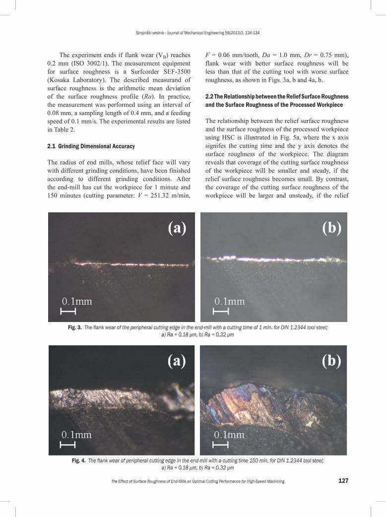
The radius of end mills, whose relief face will vary with different grinding conditions, have been finished according to different grinding conditions. After the end-mill has cut the workpiece for 1 minute and 150 minutes (cutting parameter: V = 251.32 m/min,

F = 0.06 mm/tooth, Da = 1.0 mm, Dr = 0.75 mm), flank wear with better surface roughness will be less than that of the cutting tool with worse surface roughness, as shown in Figs. 3a, b and 4a, b.

2.2 The Relationship between the Relief Surface Roughness and the Surface Roughness of the Processed Workpiece

The relationship between the relief surface roughness and the surface roughness of the processed workpiece using HSC is illustrated in Fig. 5a, where the x axis signifes the cutting time and the y axis denotes the surface roughness of the workpiece. The diagram reveals that coverage of the cutting surface roughness of the workpiece will be smaller and steady, if the relief surface roughness becomes small. By contrast, the coverage of the cutting surface roughness of the workpiece will be larger and unsteady, if the relief

Fig. 3. The flank wear of the peripheral cutting edge in the end-mill with a cutting time of 1 min. for DIN 1.2344 tool steel; a) Ra = 0.18 μm, b) Ra = 0.32 μm

Fig. 4. The flank wear of peripheral cutting edge in the end-mill with a cutting time 150 min. for DIN 1.2344 tool steel; a) Ra = 0.18 μm, b) Ra = 0.32 μm



surface roughness becomes large. The difference between both average surface roughnesses is 0.131 μm. As shown in Figs. 5b and c, even under other cutting conditions, the experiments still result in the same outcome. Thus it has been proved that the relief surface roughness is an important parameter in high-speed milling.

3 EXPERIMENTAL DISIGN AND RESULTS

3.1 Experimental Design

The influences of the surface roughness of the relief face on the cutting performance using HSC and the optimal level determination of processing parameters will be analysed. The cutting performance of the end-mill for HSC is relevantly correlated with the processing parameters (the surface roughness of the relief face (A), cutting speed (B), feed per tooth (C), axial cutting depth (D), and radial cutting depth (E)), which are regarded as controllable factors in the study. The selected processing parameters and their assigned value of the level are listed in Table 3. Here, the grinding parameters of A1 (0.23±0.03 μm) in this study are as follows: grit size of the diamond wheel = M25, grinding speed = 1650 m/min, and feed speed = 600 mm/min. The same parameters of A2 (0.43±0.02 μm) are as follows: grit size of the diamond wheel = D46, grinding speed = 1650 m/min, and feed speed = 900 mm/min. The tool grinding times are 621 and 405 s. Here A1 and A2 indicate the roughnesses of the tool coated with TiAlN after grinding.

Table 3. Processing parameters and their levels

Symbol Processing parameter Level 1 Level 2 Level 3

ASurface roughness of the relief face [μm]

0.23±0.03 0.43±0.02

BCutting speed [m/min]

251.32 351.85 452.38

CFeed per tooth [mm/tooth]

0.02 0.06 0.10

DAxial cutting depth [mm]

0.50 1.00 1.50

ERadial cutting depth [mm]

0.50 0.75 1.00

Selecting the orthogonal array involves the total degree of freedom of the processing parameters. The degree of freedom is defined as the number of comparisons among the process parameters required to optimise the parameters. Here one processing parameter is available for 2 levels and four processing parameters are suitable for 3 levels. This experimental arrangement does not consider the interaction among the processing parameters. The freedom of the processing parameter is the level minus one. Here, the total freedoms are 9 so the L18 orthogonal array is utilized for the experimental plan. Table 4 shows the configuration of processing parameters according to the L18 orthogonal array.

The tool life and wear rate of the cutting edge are analysed. The cutting performance can be evaluated according to the wear rate, which can be classified as peripheral and end wear rate. The metal removal rate governs the removal volume during cutting. A high metal removal rate is generally better, but decreases the tool life. Therefore, in this study an optimal method for processing parameters with a minimum

a) b) c)

0.00

0.10

0.20

0.30

0.40

0.50

0.60

0 50 100 150 200

Ra

(μm

)

Cutting time (min)

Relief face Ra=0.32(μm)


0.00

0.10

0.20

0.30

0.40

0.50

0.60

0 20 40 60 80 100R

a (μ

m)

Cutting time (min)

Relief face Ra=0.41(μm)Relief face Ra=0.31(μm)

0.00

0.10

0.20

0.30

0.40

0.50

0.60

0 20 40 60 80

Ra

(μm

)

Cutting time (min)



Fig. 5. Effect of cutting time on the surface roughness of the workpiece; a) cutting parameters: V = 251.32 m/min, F = 0.06 mm/tooth, Da = 1.0 mm, Dr = 0.75 mm; b) cutting parameters: V = 351.85 m/min, F = 0.02 mm/tooth, Da = 1.0 mm, Dr = 1.0 mm;

c) cutting parameters: V = 452.38 m/min, F = 0.1 mm/tooth, Da = 1.0 mm, Dr = 0.5mm



wear rate and maximum metal removal rate has been proposed. The peripheral wear rate (TWR1), end wear rate (TWR2), and metal removal rate (MRR) are defined in the following equations.

TWR

average width of flank wearof peripheral cutting edg1= ee

cutting time

, (6)

TWR

average width of flank wearof end cutting edge

cutti2 =

nng time , (7)

MRR total metal removal volumscutting time

=

. (8)

3.2 Experimental Results

Based on the experimental layout as illustrated in Table 4, the experiments are performed in series and each specific experiment is repeated two times. The procedures are described as follows:1. The overhang length of the tools is selected at a

fixed value of 20 mm.2. The tool dynamic under test is required to be less

than 0.02 G.

3. The eperiment ends if flank wear (VB) reaches 0.2 mm (ISO 3002/1).The cutting duration and volume of metal

removal are then calculated. Peripheral and end flank wear quantity are measured using a OLYMPUS STM5-BDZ microscope. According to Eqs. (6) to (8), flank wear and metal removal rate can be analysed, with those results listed in Table 4.

4 ANALYSES AND DISCUSSION

The optimisation issue of multiple performance characteristics is analysed by using the grey relation method. Optimal design of processing parameters is described as follows:1. Experimental results converted into S/N ratio.2. Normalization of S/N ratio.3. Analysis of grey relation coefficient.4. Calculation of grey relation grade. 5. Analysis of variation (ANOVA).6. Determination of optimal level of processing

parameters.7. Conduct confirmation experiments.

4.1 Optimal Combination of the Processing Parameters

Performance characteristics are first converted into the S/N ratio using the Taguchi method. Using S/N

Table 4. Experimental layout and results

No.

Experimental layout Experimental and analysis results

A B C D ECutting Time

[min]

Flank wear rate [mm/min]×10-4

MRR [mm3/min]

TWR1 TWR21 2 1 2

1 0.24 251.32 0.02 0.50 0.50 140.39 12.77 13.77 8.05 8.08 2002 0.20 251.32 0.06 1.00 0.75 188.53 8.12 9.30 6.62 6.55 18003 0.20 251.32 0.10 1.50 1.00 156.05 13.83 13.95 9.52 9.97 60004 0.22 351.85 0.02 0.50 0.75 141.40 13.58 12.96 8.82 8.59 4505 0.25 351.85 0.06 1.00 1.00 53.03 30.08 30.55 22.58 22.77 36006 0.22 351.85 0.10 1.50 0.50 98.98 15.48 15.36 13.23 14.04 45007 0.23 452.38 0.02 1.00 0.50 80.55 23.25 22.47 14.87 15.15 8008 0.21 452.38 0.06 1.50 0.75 44.19 47.92 46.85 24.38 23.14 54009 0.25 452.38 0.10 0.50 1.00 43.18 40.99 40.53 41.11 41.46 4000

10 0.42 251.32 0.02 1.50 1.00 119.69 16.19 16.13 10.95 10.42 120011 0.45 251.32 0.06 0.50 0.50 194.43 9.86 9.76 8.49 8.59 60012 0.42 251.32 0.10 1.00 0.75 170.29 7.60 7.66 11.52 10.26 300013 0.45 351.85 0.02 1.00 1.00 79.12 24.90 23.86 11.98 13.30 120014 0.42 351.85 0.06 1.50 0.50 76.59 22.78 22.07 15.44 15.90 270015 0.43 351.85 0.10 0.50 0.75 98.98 18.36 18.41 15.81 15.81 225016 0.45 452.38 0.02 1.50 0.75 37.62 52.89 53.82 23.86 23.39 180017 0.42 452.38 0.06 0.50 1.00 53.03 33.80 33.71 21.17 21.45 240018 0.45 452.38 0.10 1.00 0.50 74.24 29.27 28.76 15.90 16.47 4000



quantity, optimal performance and minimal variance can be designed. A longer tool life generally implies a higher metal removal rate and better cutting performance. Therefore, the wear rate should be at a minimum and the metal removal rate should be at a maximum. The results in Table 4 are substituted in Eqs. (1) and (2). Table 5 lists the S/N ratio of TWR1, TWR2, and MRR. The S/N ratio can be used for performance analysis. Moreover, a higher S/N ratio should improve the performance characteristics. Based on Eq. (3), the S/N ratio in Table 5 can be normalized for a better comparison. To compare with the original sequences (ideal sequences / (1, 1, 1)), they should be converted into grey relational coefficients by Eq. (4) so that the quantities range from 0.33 to 1. A higher relationship with a distinguishing coefficient leads to a higher distinguishing coefficient. The distinguishing coefficient is normally 0.5. By using Eq. (5), Table 5 shows the grey relation grade of multiple performance characteristics. According to this table, the grey relation grade of the second group is at the maximum (0.82), implying that its multiple performance characteristic is the optimum result in 18 groups.

The grey relational grade for each level of the processing parameters is summarised and shown in Table 6. In addition, the total mean of the grey relational grade for the 18×2 experiments is also calculated to be 0.596. Basically, the larger the grey relational grade, the better the multiple performance characteristics. However, the relative importance

among the processing parameters for multiple performance characteristics still needs to be known, so that the optimal combinations of the processing parameter levels can be determined.

4.2 Analysis of Variance

Variance analysis is employed to determine the influence of processing parameters on multiple performance characteristics by a statistical method. Additionally, the F test and P test are performed to verify which end-mill for HSC process parameters significantly affects the performance characteristics. A P-value < α represents a significant difference. In addition, a larger F-value and a smaller P-value indicate more significant differences. In this study, the value of α is 0.05. Table 7 demonstrates that cutting speed (B) and feed per tooth (C) significantly affect the multiple performance characteristics, i.e. tool life and metal removal rate, because their corresponding F ratio is greater than 4.46, corresponding to the ratio of F0.05 (2, 8) and P-value less than 0.05. The surface roughness ratio of the relief face is 3.87% from the results of variance analysis, therefore, this parameter is inconspicuous in terms of the influence of the cutting performance characteristics. The relative error is 9.57% so that in this experiment there are no important factors neglected. The results are thus satisfactory. Based on the above discussion, the optimal processing parameters are as follows: the

Table 5. Optimization process of processing parameters

NoSequences of S/N ratio Normalized S/N ratio Grey relational coefficient Grey relational

gradeOrders

TWR1 TWR2 MRR TWR1 TWR2 MRR TWR1 TWR2 MRR1 -22.47 -18.13 46.02 0.72 0.89 0.00 0.64 0.82 0.33 0.60 72 -18.84 -16.37 65.11 0.93 1.00 0.65 0.88 1.00 0.59 0.82 13 -22.85 -19.78 75.56 0.69 0.79 1.00 0.62 0.70 1.00 0.77 34 -22.46 -18.80 53.06 0.72 0.85 0.24 0.64 0.77 0.40 0.60 65 -29.63 -27.11 71.13 0.29 0.33 0.85 0.41 0.43 0.77 0.54 136 -23.76 -22.70 73.06 0.64 0.60 0.92 0.58 0.56 0.86 0.66 57 -27.18 -23.53 58.06 0.44 0.55 0.41 0.47 0.53 0.46 0.48 178 -33.51 -27.52 74.65 0.06 0.30 0.97 0.35 0.42 0.94 0.57 109 -32.21 -32.32 72.04 0.14 0.00 0.88 0.37 0.33 0.81 0.50 1510 -24.17 -20.58 61.58 0.61 0.74 0.53 0.56 0.65 0.51 0.58 911 -19.83 -18.63 55.56 0.87 0.86 0.32 0.79 0.78 0.42 0.67 412 -17.66 -20.77 69.54 1.00 0.72 0.80 1.00 0.64 0.71 0.78 213 -27.74 -22.06 61.58 0.40 0.64 0.53 0.46 0.58 0.51 0.52 1414 -27.02 -23.90 68.63 0.45 0.53 0.77 0.47 0.51 0.68 0.56 1215 -25.29 -23.98 67.04 0.55 0.52 0.71 0.53 0.51 0.63 0.56 1116 -34.54 -27.47 65.11 0.00 0.30 0.65 0.33 0.42 0.59 0.45 1817 -30.57 -26.57 67.60 0.24 0.36 0.73 0.40 0.44 0.65 0.49 1618 -29.25 -24.18 72.04 0.31 0.51 0.88 0.42 0.51 0.81 0.58 8



surface roughness of relief face at level one 0.23±0.03 μm, cutting speed at level one 251.32 m/min, feed per tooth at level three 0.1 mm/tooth, axial cutting depth at level two 1.0 mm, and radial cutting depth at level two 0.75 mm.

4.3 Verification Experiments

After the optimal level of the processing parameters is obtained, improvement of the performance characteristics must then be verified by using these optimal processing parameters. Table 8 compares the results of the confirmation experiments using the optimal processing parameters (A1, B1, C3, D2, E2) obtained by the proposed method with those of the initial processing parameters (A2, B1, C2, D3, E1), as provided by Li-Hsing Precision Tool Manufacturing Company.

According to Table 8, tool life is defined as the total cutting time before the breakage of cutting edge of the tool or as the flank wear of cutting edge reaches 0.2mm (ISO 3002/1). This table also reveals a 5.37% increase in the tool life (i.e. from 169.43 to 178.53 min), a 75.62% increase in the total metal removal volumes (i.e. from 304974 to 535600 mm3),

a 66.67% increase in the metal removal rate (i.e. from 1800 to 3000 mm3/min), and a 43.14% decrease in the average surface roughness of workpiece (i.e. from 0.102 to 0.058 μm). Figs. 6a and b show the effects of cutting time on flank wear of the cutting edge under the conditions of the initial processing parameters compared with those of the final optimal processing parameters. Consequently, the verification tests reveal that the proposed algorithm for solving the optimal processing parameters decrease the average surface roughness of the workpiece and increases both the tool life and metal removal rate.

4.4 Influence of Cutting Performance on the Surface Roughness of the Relief Face

The ranges of surface roughness of the relief face for this study are from 0.23±0.03 to 0.43±0.02 [μm]. Fig. 7 shows the integrity of the cutting edge enlarged 200 fold by microscope (OLYMPUS STM5-BDZ). In addition, it recognizes the integrity of the surface roughness of the relief face on the cutting edge of the difference. Importantly, Table 6 indicates that the surface roughness of the relief face using gray relational grade analysis for the difference is 0.041. In

Table 6. Response table for the grey relational grade

Symbol Processing parameter Level 1 Level 2 Level 3 Max-Min RankingA Surface roughness of relief face 0.616 0.575 0.041 5B Cutting speed 0.703 0.572 0.512 0.191 1C Feed per tooth 0.537 0.607 0.643 0.106 2D Axial cutting depth 0.570 0.620 0.598 0.051 4E Radial cutting depth 0.591 0.630 0.567 0.063 3

Total mean value of the grey relational grade = 0.596

Table 7. Results of the analysis of variance

Symbol Processing parameter Degree of freedom Sum of square Mean square F value P value Contribution [%]A Surface roughness of relief face 1 0.008 0.008 3.238 0.110 3.87B Cutting speed 2 0.114 0.057 24.459 0.000 58.52C Feed per tooth 2 0.035 0.018 7.498 0.015 17.94D Axial cutting depth 2 0.008 0.004 1.668 0.248 3.99E Radial cutting depth 2 0.012 0.006 2.553 0.139 6.11

Error 8 0.019 0.002 9.57Total 17 0.195 100.00

F0.05(1,8) = 5.32, F0.05(2,8) = 4.46

Table 8. Confirmation test results

Processing combination

Tool life [min]Total metal removal

volumes [mm3]Metal removal rate

[mm3/min]Average surface roughness of

workpiece [μm]Optimal A1B1C3D2E2 178.53 535600 3000 0.058Initial A2B1C2D3E1 169.43 304970 1800 0.102Final gain 9.10 230630 1200 0.044



Table 7, it can be seen that the surface roughness ratio of the relief face reveals a 3.87% difference from the results of the variance analysis.

By comparing the results of the optimal processing parameters (A1 B1 C3 D2 E2) with those of the No.12 experimental processing parameters (A2 B1 C3 D2 E2), there is a 4.84% increase in tool life (i.e. from 170.29 to 178.53 min). From Figs. 6a to c, the effect of cutting time on flank wear of the cutting edge and surface roughness of workpiece under the conditions of comparing the No.12 experimental processing parameters with those of the final optimal processing parameters can be summarized. Therefore, the surface roughness of the relief face parameter is inconspicuous in terms of the influence of the cutting performance characteristics. There are two explanations for this result.

First, Figs 6a and b demonstrate that the surface roughness of the relief face has no significant

influence on flank wear in HSC before 135 min of continuous cutting. In addition, as indicated in the Fig. 6c, the surface roughness of the relief face will essentially affect the surface roughness of the processed workpiece, i.e. with 48.21% decrease in the average surface roughness of workpiece (from 0.112 to 0.058 μm). However, the smaller surface roughness of the relief face (0.22 μm) will induce less flank wear and less surface roughness of the workpiece.

In terms of tool grinding, the surface roughness of relief face for this study will be set at 0.23±0.03 and 0.43±0.02 μm and the corresponding tool grinding times are 621 and 405 s, respectively. As mentioned above, grinding with the surface roughness of relief face at level 1 (0.23±0.03 μm) for the end-mill will lead to a 53.33% increase in grinding cost, but only a 4.84% increase in tool life. Due to a slight effect on cutting performance characteristics of the rough

a) b) c)

0.00

0.05

0.10

0.15

0.20

0.25

0.30

0 70 140 210

Flan

k w

ear

(mm

)

Cutting time(min)

Initial designExperimental No.12Optimal design

0.00

0.05

0.10

0.15

0.20

0.25

0.30

0 70 140 210Fl

ank

wea

r (m

m)

Cutting time (min)


0.00

0.10

0.20

0.30

0.40

0.50

0 70 140 210

Ra

(μm

)

Cutting time(min)


Fig. 6. Effect of cutting time on cutting performance; a) flank wear of the peripheral cutting edge, b) flank wear of the end cutting edge, c) surface roughness of the workpiece

a) b)

Fig. 7. The cutting edge integrity of surface roughness of the relief face; a) Ra=0.23 μm, b) Ra=0.43 μm



machining, A2 grinding conditions can be used to improve tool grinding efficiency.

5 CONCLUSIONS

From the above descriptions and analyses, the optimal processing parameters of DIN 1.2344 tool steel will be determined by grey relational analysis. Clearly, the optimal results are only given under conditions of HSC in DIN 1.2344 tool steel. The results can be summarized as follows.1. The surface roughness of the relief face levels

are set at 0.23±0.03 and 0.43±0.02 μm for this study. According to the variance analysis results, the surface roughness of the relief face of an end-mill slightly influences rough machining in HSC for DIN 1.2344 tool steel. In addition, it will essentially affect the surface roughness of the workpiece, there being a decline of 0.054 μm in the average surface roughness of workpiece (i.e. from optimal processing parameters to No.12 experimental processing parameters). Therefore, A2 grinding conditions (grit size of diamond wheel = D46, grinding speed = 1650 m/min, and feed speed = 900 mm/min) can be used to improve tool grinding efficiency.

2. Based on an analysis of variance, the major controllable factors significantly affecting multiple performance characteristics, i.e. tool life and metal removal rate, are cutting speed and feed per tooth with a desired total contribution of 76.46%.

3. The optimal combination obtained from the proposed method is the processing condition with a surface roughness of the relief face of 0.23±0.03 μm, cutting speed of 251.32 m/min, feed per tooth of 0.1 mm/tooth, axial cutting depth of 1.0 mm, and radial cutting depth of 0.75 mm. The corresponding verification tests indicate an improvement of 9.1 min in tool life, 1200 mm3/min in metal removal rate, 230616 mm3 in total metal removal volumes, and 0.044 μm in average surface roughness of workpiece from the initial parameters to the optimal parameters.

6 REFERENCES

[1] Li, L., He, N., Wang, M., Wang, Z.G. (2002). High speed cutting of Inconel 718 with coated carbide and ceramic inserts. Journal of Materials Processing Technology, vol. 129, no. 1-3, p. 127-130, DOI:10.1016/S0924-0136(02)00590-3.

[2] Dolinsek, S., Sustarsic, B., Kopac, J. (2001). Wear mechanisms of cutting tools in high speed cutting process. Wear, vol. 250, no. 1-12, p. 349-356, DOI:10.1016/S0043-1648(01)00620-2.

[3] Malkin S. (1989). Grinding Technology: Theory and Applications of Machining with Abrasives. Society of Manufacturing Engineers, Michigan.

[4] Shaji, S., Radhakrishnan, V. (2003). Analysis of process parameters in surface grinding with graphite as lubricant based on the Taguchi method. Journal of Materials Processing Technology, vol. 141, no. 1, p. 51-59, DOI:10.1016/S0924-0136(02)01112-3.

[5] Yin, L., Spowage, A.C., Ramesh, K., Huang, H., Pickering, J.P., Vancoille, E.Y.J. (2004). Influence of microstructure on ultraprecision grinding of cemented carbides. International Journal of Machine Tools and Manufacture, vol. 44, no. 5, p. 533-543, DOI:10.1016/j.ijmachtools.2003.10.022.

[6] Kwak, J.S. (2005). Application of Taguchi and response surface methodologies for geometric error in surface grinding process. International Journal of Machine Tools and Manufacture, vol. 45, no. 3, p. 327-334, DOI:10.1016/j.ijmachtools.2004.08.007.

[7] Nguyen, T.A., Butler, D.L. (2005). Simulation of precision grinding process, Part 2: Interaction of the abrasive grain with the workpiece. International Journal of Machine Tools and Manufacture, vol. 45, no. 11, p. 1329-1336, DOI:10.1016/j.ijmachtools.2005.01.006.

[8] Park, S.H. (1996) Robust Design and Analysis for Quality Engineering. Springer, London.

[9] Dhavlikar, M.N., Kulkarni, M.S., Mariappan, V. (2003). Combined Taguchi and dual response method for optimization of a centerless grinding operation. Journal of Materials Processing Technology, vol. 132, no. 1-3, p. 90-94, DOI:10.1016/S0924-0136(02)00271-6.

[10] Korkut, I., Kucuk, Y. (2010). Experimental analysis of the deviation from circularity of bored hole based on the taguchi method. Strojniški vestnik - Journal of Mechanical Engineering, vol. 56, no. 5, p. 340-346.

[11] Çiçek, A., Kıvak, T., Samtaş, G. (2012). Application of taguchi method for surface roughness and roundness error in drilling of AISI 316 stainless steel. Strojniški vestnik - Journal of Mechanical Engineering, vol. 58, no. 3, p. 165-174, DOI:10.5545/sv-jme.2011.167.

[12] Motorcu, A.R. (2010). The optimization of machining parameters using the taguchi method for surface roughness of AISI 8660 hardened alloy steel. Strojniški vestnik - Journal of Mechanical Engineering, vol. 56, no. 6, p. 391-401.

[13] Saglam, H., Yaldiz, S., Unsacar, F. (2007). The effect of tool geometry and cutting speed on main cutting force and tool tip temperature. Materials and Design, vol. 28, p. 101-111, DOI:10.1016/j.matdes.2005.05.015.

[14] Lin, J.L., Lin, J.F. (2006). Grey theory applied to evaluate the tribological performance of the a-C:H(N) coating films prepared by differing the nitrogen content and the film thickness. The International Journal of

http://dx.doi.org/10.1016/S0924-0136(02)00590-3

http://dx.doi.org/10.1016/S0924-0136(02)00590-3

http://dx.doi.org/10.1016/S0043-1648(01)00620-2

http://dx.doi.org/10.1016/S0924-0136(02)01112-3

http://dx.doi.org/10.1016/j.ijmachtools.2003.10.022




http://dx.doi.org/10.1016/S0924-0136(02)00271-6

http://dx.doi.org/10.5545/sv-jme.2011.167

http://dx.doi.org/10.1016/j.matdes.2005.05.015



Advanced Manufacturing Technology, vol. 27, no. 9-10, p. 845-853, DOI:10.1007/s00170-004-2294-1.

[15] Panneerselvam, K., Pradeep, K. Asokan, P. (2012). Optimization of end milling parameters for glass fiber reinforced plastic (GFRP) using grey relational analysis. Procedia Engineering, vol. 38, p. 3962-3968, DOI:10.1016/j.proeng.2012.06.453.

[16] Ilo, S., Just, Ch., Xhiku, F. (2012). Optimisation of multiple quality characteristics of hardfacing using grey-based taguchi method. Materials and Design, vol. 33, p. 459-468, DOI:10.1016/j.matdes.2011.04.050.

[17] Sahoo, A.K., Baral, A.N., Rout, A.K., Routra, B.C. Multi-objective optimization and predictive modeling of

surface roughness and material removal rate in turning using grey relational and regression analysis. Procedia Engineering, vol. 38, p. 1606-1627.

[18] Palanikumar, K. (2011). Experimental investigation and optimisation in drilling of GFRP composites. Measurement, vol. 44, p. 2138-2148, DOI:10.1016/j.measurement.2011.07.023.

[19] Ross, P.J. (1988). Taguchi Techniques for Quality Engineering. McGraw-Hill, New York.

[20] Deng, J.L. (1989). Introduction to Grey system. The Journal of Grey System, vol. 1, no. 1, p. 1-24.

http://dx.doi.org/10.1007/s00170-004-2294-1

http://dx.doi.org/10.1016/j.proeng.2012.06.453

http://dx.doi.org/10.1016/j.matdes.2011.04.050

http://dx.doi.org/10.1016/j.measurement.2011.07.023

http://dx.doi.org/10.1016/j.measurement.2011.07.023

Documents

DOI:10.5545/sv-jme.2012.677 The Effect of Surface ... coating technology, tool geometry design, ... and selection of ... including pressure die casting tools, extrusion tools, forging