DOI: 10.1002/((please add manuscript number)) Article type: Communication

A unified approach for patterning via frontal photopolymerization

Alessandra Vitale,* Matthew G. Hennessy, Omar K. Matar, and João T. Cabral*

Dr. A. Vitale, Dr. M. G. Hennessy, Prof. O. K. Matar, Dr. J. T. CabralDepartment of Chemical Engineering, Imperial College London, South Kensington Campus, London SW7 2AZ, U.K.E-mail: a.vitale@imperial.ac.uk; j.cabral@imperial.ac.uk

Keywords: frontal photopolymerization, 3D patterning, spatio-temporal model, polymer networks

The ability to rapidly pattern polymeric microstructures with prescribed shape and thickness

is desirable for a wide range of applications,[1, 2] including biotechnology,[3, 4] electronics and

optics,[5-7] coating and adhesives,[8] and surface science.[9, 10] Photopolymerization is ubiquitous

in lithography,[11] as well as 3D rapid prototyping[12] and additive manufacturing,[13] and is thus

a pillar of micro and nanofabrication. Photoinitiated polymerization of multifunctional

monomers is an efficient method to synthesize highly crosslinked polymer networks[14, 15] at

room temperature, without the use of solvents, and with very short conversion times. A

powerful type of photoinduced polymerization for three-dimensional patterning is the so-

called frontal photopolymerization (FPP).[16-19] FPP is a process in which a narrow

polymerization zone―a front― develops and propagates as a planar travelling wave into the

monomer material, driven by an external light source. The sharp interfacial profile, between

polymer network and monomer bath, emanates from the surface closest to the illuminating

source and invades the uncrosslinked medium. Frontal photopolymerization is directional and

can be controllably initiated and stopped using collimated light exposure, which is

advantageous from a manufacturing perspective. Further, it enables multi-level patterning by

spatially varying illumination, without resorting to several illumination and alignment steps. 1

FPP is based on free radical photopolymerization of multifunctional monomers, which is the

most widely used type of UV curing as it can be controlled both spatially and temporally

(differently from cationic polymerization, in which the chain reaction continues to proceed

even in the absence of illumination).[20] Both acrylic[21] and thiol-ene[22] systems can

polymerize by a radical-mediated mechanism. FPP’s fabrication versatility has been

demonstrated in numerous applications, from the synthesis of microparticles[23] to

manufacturing of three-dimensional microfluidic devices[16] and hybrid materials.[24]

Many theoretical studies on photoinduced polymerization, and specifically on FPP, have

resulted in a range of mathematical models to predict spatio-temporal photopolymerization

kinetics,[25, 26] both for acrylate[27] and thiol-ene[28-30] photocurable systems. Explicit models

accounting for various reaction steps (minimally, photoinitiation, propagation and

termination) generally require numerical computation and a large number of parameters,

many of which cannot be measured experimentally. Coarse-grained models based on physical

observables,[16, 18, 31] on the other hand, benefit from greater simplicity, thus making them

amenable to both mathematical analysis and predictive FPP fabrication. A well-established

minimal FPP model[16, 18] describes the spatio-temporal evolution of the solidification network

by coupling an equation of motion for a monomer-to-polymer conversion order parameter

(dimensionless and defined 0≤≤1, from neat monomer to polymerization completion), and a

generalized Beer-Lambert law to compute the light intensity throughout the process (further

details are reported in the Supporting Information). In the absence of mass and thermal

diffusion, the shape-invariant conversion profile can be solved to yield:[17]

ϕ ( z , t )=1−exp[−K I 0 exp (−μz ) t ] (1)

where z is the direction normal to the illuminated surface (which is z≡0), t is the UV exposure

time, K is a material constant corresponding to an effective reaction conversion rate, I0 is the

light intensity at the surface, and is the attenuation coefficient (taken to be constant in

photoinvariant polymerization). Equation 1 describes the non-linear monomer-to-polymer 2

conversion profile of within the material. The front position zf, corresponding to the

solidified thickness, can be readily computed by defining a critical threshold conversion

fraction c required to form a network, i.e. zf≡z(=c), resulting in:

z f=ln [K I 0 t / ln (1/(1−ϕc)) ]

μ(2)

which is therefore predicted to grow logarithmically with time t. Such models have recently

been extended to explicitly account for changing optical properties, for instance during photo-

bleaching or darkening,[18, 31] mass[31] and thermal[32] diffusion.

Experimental[19, 33, 34] studies of FPP are relatively limited and focus only on restricted and

selected photopolymerizing materials, such as acrylates[24, 33, 35, 36] and thiol-ene optical

adhesives.[16, 17, 19] A unified FPP patterning strategy, robust to different monomer systems, and

applicable to the fabrication of solid polymer networks with well-defined dimensions, is

evidently lacking and is, thus, the main purpose of our work.

We comparatively investigate the FPP process for a range of representative thiol-ene and

acrylate photocurable systems, establishing the factors governing the profile propagation and

the conditions relevant for pattern formation.

A representative FPP experimental setup is depicted in Figure 1. The planar polymerization

wave emanates from the top, illuminated, transparent surface, which anchors the growing

solid network. The illumination source is typically a collimated UV light lamp. FPP

patterning is generally modulated through a photomask, readily yielding patterns with desired

shapes, although grey-scale masks and reconfigurable stereo-lithographic setups are also

possible. After light exposure and development to remove the uncured material, a crosslinked

polymer sample with thickness zf is obtained. The associated c corresponds to the gel point of

the specific system: above c the network is insoluble upon development, while below c it is

soluble. Generally, the governing parameter is the light dose d, which is defined as the

product of light intensity and exposure time (i.e., d≡I0×t), and Equation 2 thus predicts the

3

thickness zf to grow logarithmically with d. A critical UV dose dc is, however, required for the

solid front to form and start propagating from the illuminated surface. In the framework of our

minimal FPP model,[16, 18] this threshold dose dc corresponds to that required to reach the

critical conversion fraction c; further, the inverse of the slope of the thickness curve on a

logarithmic scale, depicted in Figure 1, corresponds to the optical attenuation coefficient of

the polymerizing material.

Figure 1. Schematic of the FPP experimental setup showing the photopolymerization front propagation from the UV illuminated surface. A photomask defines the lateral pattern shape. Thermocouples were directly embedded to measure the local temperature during reaction. The light-driven solidification wave propagates in a planar fashion from the illuminated surface into the monomer medium. The extent of monomer-to-polymer conversion within the network has a sigmoidal shape profile, moving along z with increasing light exposure dose d. The sample thickness zf increases logarithmically with dose d, after a critical value dc has been exceeded. The threshold dose dc corresponds to a critical conversion fraction c.

We select different thiol-ene and (meth)acrylic photocurable systems for this FPP study:

1,3,5-triallyl-1,3,5-triazine-2,4,6(1H,3H,5H)-trione (triallyl) and trimethylolpropane diallyl

ether (diallyl), both mixed with pentaerythritol tetrakis(3-mercaptopropionate), as model

thiol-ene systems, and poly(ethylene glycol) diacrylate (diacrylate) and trimethylolpropane

trimethacrylate (trimethacrylate) as model acrylic systems. The radical photoinitiator (PI) was

the same for all materials and its concentration kept constant for consistency (unless stated

otherwise). The chemical structures of the monomers are reported in Supporting Information,

Figure S1. For comparison, our study includes a commercial thiol-ene resin (NOA 81),

commonly employed as an adhesive and negative photoresist, whose FPP propagation

kinetics has been previously reported.[16, 17, 19] The photopolymerization kinetics (conversion vs 4

time) for all systems investigated is shown in Figure S2 of Supporting Information. As the

existence of a photopolymerization front is the defining aspect of FPP, contrasting it to

conventional photopolymerization, we first report on the front kinetics by measuring the

thickness of UV cured samples following illumination and removal of the residual liquid

monomer (i.e. development). All the studied systems exhibited a well-defined polymerization

front with a logarithmic growth in thickness with increasing irradiation time, or dose (Figure

2a and b). The equivalence between does and time, for this irradiation intensity range, is

demonstrated in Figure S3 in Supporting Information. The exposure dose is found to finely

control the front position within the reactive mixture in all cases, yielding film thicknesses

ranging from few m to mm. Figure 2c shows that, as expected, polymerization kinetics

varies with monomer chemistry. For instance, each monomer system exhibits a distinct value

of critical dose dc for the onset of the polymerization reaction, due to the different radical

reactivity. However, front kinetics are not found to be affected by the possible shrinkage of

the UV curable systems (Figure S3 in Supporting Information). According to our minimal

model, whose key results are illustrated in Figure 1, the inverse of the slope of curves in

Figure 2c is set by the optical attenuation coefficient of the system, which can be

easily―and independently―measured via the material’s light transmission. From the

experimental data reported in Figure 2, remains nearly constant within the dose range

considered, effectively corresponding to photoinvariant polymerization conditions.

Figure 2d demonstrates how FPP kinetics can be tuned through the attenuation coefficient ,

by modifying the absorbing properties of the material, for instance, via the addition of a filler.

As expected, the log propagation slope (but not the critical onset dc) is readily tuned. The

variation of the photoinitiator concentration has instead a double effect on FPP propagation

and thus on the final sample thickness zf (Figure 2e), as it impacts both absorption of incident

light and polymerization rate (via the radical formation rate). As such, by increasing PI

concentration increases, as the number of absorbing species in the reactive mixture is 5

enhanced (corresponding to a decrease in log slope); however, dc decreases due to the

simultaneous increase of reaction kinetics (i.e. increasing the effective polymerization rate

constant K).

Figure 2. Sample thickness zf dependence on UV dose d, for thiol-ene (a) and acrylic (b) systems. (c) Logarithmic growth of zf with dose, with proportionality constant 1/. The attenuation coefficient values are 3.02, 0.38, 0.53, 0.44, and 0.59 mm-1 for NOA 81, triallyl, diallyl, diacrylate and trimethacrylate, respectively. In (d) and (e), results on the modification of absorbing properties and reaction kinetics parameters for diacrylate by adding a filler (d) and by changing the photoinitiator (PI) concentration (e) are reported. The absorbing filler is TiO2, used in the range 0‒2 wt.%. The PI concentration is 0.5 and 1 wt.%.

FPP differs in nature from thermal and isothermal frontal polymerizations, which are

autocatalytic reaction processes.[37] Although these polymerization methods also develop

wavelike polymerization fronts, their propagation is heat-driven and (self-)sustained by the

thermal energy released from the exothermic polymerization reaction or by a local change in

mobility that disfavors termination (Trommsdorff-Norrish effect).[37, 38] Such propagating

fronts thus continue travelling after ignition, in the absence of an external field. By contrast,

FPP is not autocatalytic: the polymerization is initiated by photocleavage of the photoinitiator,

and the front is then driven forward by the continuous light flux. The reaction can thus be

6

stopped and restarted as desired (Supporting Information, Figure S4), simply by switching on

and off the UV irradiation, which is advantageous for spatial control in fabrication processes.

However, since photopolymerization reactions are generally strongly exothermic, it appears

necessary to consider possible thermal effects in FPP propagation. The spatio-temporal

temperature profiles of our model FPP systems are reported in Figure 3. A set of

thermocouples embedded within the reaction medium (illustrated in the inset of Figure 3a)

measured the temperature at fixed locations (z*) during front propagation. Depending on the

functionality of the monomers and the exothermicity of the polymerization reaction, we

divide the systems into three groups: thiol-ene athermal (NOA 81), thiol-ene thermal (diallyl

and triallyl), and acrylate (diacrylate and trimethacrylate). Faster polymerizations were

generally found to be most exothermic and resulted in a larger temperature rise during FPP.

Indeed, such temperature increase could in turn speed up the travelling front proceeding by

accelerating chain propagation. For all thermal systems, by following the temperature

variation at a reference position (z*), we find that, during irradiation, the temperature first

increases significantly ahead of the approaching polymerization front, reaches a maximum,

and then decreases again after the front passes, beyond the fixed measurement point (Figure

3b and Figure S5 in Supporting Information). It is worth noting that during this ‘heat rush’ the

maximum temperature does not correspond to the front position (the temperature at the front

is indicated with a red star in Figure 3b); rather, the maximum generally occurs behind the

front, due to continued polymerization and crosslinking and, hence, heat generation in this

region. Figure 3c reports the temperature profile at zf (i.e., at the front position) during

photopolymerization as a function of light dose. Once the exposure dose exceeds dc, the

temperature at the front is found to remain nearly constant.

7

Figure 3. (a) Temperature profiles for different polymeric systems during photopolymerization. Temperature was measured with a thermocouple embedded at a distance z*=1.3 mm from the illuminated surface. Red stars correspond to the temperature at the front position (i.e., zf=z*). (b) Temperature evolution with UV dose for triallyl at three distances from the sample surface (z*1=0.5 mm, z*2=1.3 mm, z*3=3 mm). Red stars correspond to the temperature at the front position. (c) Variation of temperature at the front zf during photopolymerization reaction (i.e., increasing the UV dose, with d>dc) of the triallyl system.

While thermal effects can certainly impact FPP kinetics[32] (discussed below), we find that

even temperature rises (ΔT) of up to 30°C do not disrupt appreciably the log kinetics shown in

Figure 2. We next turn our attention to the spatio-temporal monomer-to-polymer conversion

profiles during photopolymerization, which were experimentally probed by Fourier

Transform Infrared (FT-IR) spectroscopy and computed numerically using FPP models.[16, 18,

32] For the thiol-ene athermal system, profiles follow our minimal FPP model:[16, 19] as shown

8

in Figure 4a, all experimental data are well described by Equation 1. The critical conversion

c at the solid/liquid interface is found to be 0.05, as estimated by FT-IR experiments in

attenuated total reflection (ATR) mode on the top surface of the crosslinked sample. This

value is considerably lower than the gel point conversion expected for multifunctional thiol-

ene systems, likely due to the large oligomeric fraction of the commercial NOA 81 reactive

mixture. Since the value of can be independently measured and remains constant, the model

has K as the sole fitting parameter. For this thiol-ene athermal system, the value of K remains

approximately constant during exposure (i.e. with increasing UV dose) and equal K0 (see inset

in Figure 4a). We define K0 as the photopolymerization kinetics constant at the onset of the

reaction, which can hence be related to the experimental critical values for solidification,

defined above and measured directly:

K0=ln( 1

1−ϕc )dc

(3)

As shown in Figure 4b and c, the profiles of thiol-ene thermal systems (both triallyl and

diallyl) can be fitted remarkably well by a simple thermal FPP model which we have reported

recently[32] (fitting results with minimal FPP model and a brief description of the model

considering thermal effects are reported in the Supporting Information, Figure S6). Thermal

effects must be taken into account explicitly due to the strong exothermic nature of the

process. However, even in this case, the value of required for the fitting process corresponds

to the one independently measured from the material‘s light transmission. In the thermal-

modified FPP model,[32] K is assumed to increase with temperature following an Arrhenius

law, describing how the reaction exothermicity improves the polymerization rate and speeds

up the front propagation. The critical c values are measured to be 0.48 and 0.64 for triallyl

and diallyl, respectively, as expected for systems where trifunctional and difunctional enes are

polymerized in equimolar ratio with a tetrafunctional thiol monomer.

9

The experimental profiles for the acrylic systems could only be fitted using both K and as

free fitting parameters (Figure 4d and e). Further details on other fitting results are reported in

the Supporting Information (Figure S7 and S8). Qualitatively, the conversion profiles of the

acrylic systems at the surface layer appear to reach completion but then drop beyond a certain

depth z faster than expected from our FPP models.[16, 18, 31, 32] This drop could be associated

with the fact that, after vitrification of the material, the propagation reaction becomes

diffusion controlled during the autodeceleration regime. Also in this case, K follows the

temperature evolution measured during FPP. We find that the effective values of K and

required to describe the profiles gradually approach K0 and 0 with increasing exposure time

(see Figure 4f), with the attenuation coefficient 0 corresponding to the directly measured

value of during photopolymerysation. We tentatively propose that, with increasing dose, the

system eventually approaches its ‘equilibrium’ profile while, at lower doses (or times), the

propagation is limited by the crosslinking stage (due to low radical mobility). For the

diacrylate and trimethacrylate systems, the measured c values are 0.24 and 0.12, respectively.

As expected, c decreases with increasing monomer functionality, and acrylates have a

considerably lower gel point compared to thiol-enes, which exhibit a delayed gelation due to

the their specific photopolymerization mechanism, which proceeds via alternating

propagation and chain transfer reactions.

Evidently, explicit theoretical polymerization models could be attempted for fitting the

experimental profiles of acrylic systems, accounting for photochemical reaction details

including initiator photolysis, chain initiation, propagation, transfer and termination.

However, the large number of model parameters required and the limited predictive power

from a patterning fabrication point of view lead us to consider an alternative approach.

10

Figure 4. Conversion profiles along the sample depth z for increasing UV dose d for different studied systems. (a) Extent of conversion dependence on z and d for thiol-ene athermal system NOA 81. Photopolymerization was performed with a dose range of 280‒4030 J m-2. Dots are experimental data, while solid lines are minimal FPP model fits (Equation 1). The inset details the values of the fitting parameter K, compared to the initial K0. (b) and (c) show the profiles for thermal thiol-ene systems: triallyl (b) and diallyl (c). The UV dose used is in the range 90‒470 J m-2 for triallyl, and 120‒370 J m-2 for diallyl. Dots are experimental data, while solid lines represent the thermal-modified FPP fits.[32] The insets detail the evolution of the fitting parameter K with UV dose. The kinetics constant K is found to vary during photopolymerization following the temperature of reaction. (d) and (e) depict the monomer-to-polymer conversion as a function of z and d for acrylic systems: diacrylate (d) and trimethacrylate (e). The dose range was 180‒740 J m-2 for diacrylate, and 1470‒5530 J m-2 for trimethacrylate. Points are experimental data, while dashed lines are model fits, conducted with free K and parameters. The black dotted line is the fitting of the experimental data series of at the highest explored dose with the fixed measured 0 value. (f) Values of fitting parameters K and as a function of UV dose for diacrylate, showing their approaching to K0 and 0 respectively.

By inspection of the experimental curves reported in Figure 2 and our minimal FPP model

equations, we obtain a remarkable collapse of all data into a single master curve, shown in

Figure 5a, which holds for all studied systems. The key feature of this curve is that it

accurately describes the relationship between patterned thickness and light exposure,

requiring only readily measurable observables, which can be used as processing parameters.

Specifically, can be rapidly estimated from prior transmittance measurements, i.e. using the

Beer-Lambert law of a section of known material thickness; K0 depends on dc by Equation 3,

and c corresponds to the macroscopic gelation point of the UV curable system, both 11

measurable directly by the critical dose for incipient solidification and/or FT-IR experiments.

Thus, the master curve of Figure 5 fully and self-consistently determines pattern fabrication,

as the important parameters to be controlled are the final pattern thickness zf and the exposure

dose d.

Since the master curve rests upon the minimal FPP model, whose assumptions (viz. athermal

reaction and no mass/heat transfer) are not strictly valid for all systems, a justification for

such level of agreements seems in order. We therefore simulate thermal effects on FPP (inset

of Figure 5a) to establish the range of applicability of this master curve: exothermic reactions

with ΔT≳50 °C (and activation energy Ea=10 kJ mol-1, representative for this class of

systems) are needed for significant departures from linearity. As for all measured systems

ΔT<30 °C, this condition is met and the level of agreement is thus outstanding (additional

details in Supporting Information, Figure S9). The relatively small temperature rises in the

studied FPP systems suggest that thermal instabilities (e.g. spin modes) are unlikely, and the

propagating fronts thus remain planar (see Supporting Information). Also, the shrinkage

induced by the photopolymerization reaction does not influence the universality of the frontal

growth kinetics shown in Figure 5a (see Supporting Information). Further, while the profile

for the acrylate systems (Figure 4d and e) departs from the minimal FPP prediction, the

interplay between the evolving and K results in a time-dependent intersection of and c

that nonetheless closely reflects that of the model. The validity of the approach is next

confirmed in practice.

Using this process control framework, we fabricated polymeric patterns from all studied

systems according to the master curve to yield patterns of prescribed thickness. The lateral

shape is set by the photomask geometry, which does not influence the final pattern thickness

(Figure S10 of Supporting Information). Selected pattern examples are shown in Figure 5b.

12

Figure 5. Master curve for the prediction of final polymeric pattern thickness. (a) Curve representing zf (the final pattern thickness zf, normalized by the material attenuation coefficient ) as a function of ln(dK0/ln(1/(1-c))≡ln(d/dc) for all studied systems, showing collapse of all measurements reported in Figure 2. The x axis of the master curve includes only readily measurable variables: d is the exposure dose, K0 depends on the threshold dc value by Equation 3, and c corresponds to the gel point of the photopolymerizing system. The inset depicts the effect of temperature rise during polymerization for selected ΔT (ranging from 0 to 80°C) as predicted by a model of thermal FPP processes (additional details in Supporting Information). (b) Examples of patterns, obtained with parameters predicted from (a) for diallyl, triallyl, diacrylate, and trimethacrylate monomers, as well as a dense multilevel thiol-ene (NOA81) array. The scale bar is 500 m.

In conclusion, we demonstrate a general and exceptionally well-controlled patterning

approach for photocurable monomers based on the understanding of frontal

photopolymerization reaction kinetics. Our strategy is demonstrated using a range of thiol-ene

and acrylic systems UV cured by FPP, which precisely defines the pattern thickness and

enables multi-level patterning by light modulation. Our minimal FPP model can describe the

evolution of the front profile―the key for quantitative patterning―with high accuracy for all

free radical systems, even when not all model assumptions are strictly valid, which we

rationalize in terms of the impact of physico-chemical (e.g. thermal, optical) effects in the

solidification front kinetics. The model yields a simple master relationship for predictive

pattern control via FPP, which is entirely based on readily measurable parameters. FPP

patterning becomes trivial using this unified approach and holds for all systems investigated

13

so far, becoming hence ideally suited for a wide range of applications such as flexible

electronics, biotechnology, and advanced coatings.

Experimental Section

Materials and methods: 1,3,5-Triallyl-1,3,5-triazine-2,4,6(1H,3H,5H)-trione (triallyl),

trimethylolpropane diallyl ether (diallyl), pentaerythritol tetrakis(3-mercaptopropionate),

poly(ethylene glycol) diacrylate (diacrylate) with a molecular weight of 700 g mol-1, and

trimethylolpropane trimethacrylate (trimethacrylate) were purchased from Sigma-Aldrich and

used as received. Thiol-ene formulations were prepared with an equimolar amount of thiol

and allyl reactive groups. Monomers were added to 1 wt.% photoinitiator 2-hydroxy-2-

methyl-1-phenyl-propan-1-one (Sigma-Aldrich) to obtain the final photocurable reactive

mixtures. The thiol-ene based optical adhesive NOA81 was obtained from Norland Products.

Titania (Aeroxide® TiO2 P25) was purchased from Degussa Evonik, and Sylgard 184 PDMS

elastomer kit from Dow Corning. All other chemicals were obtained from VWR Chemicals.

The photocurable reactive mixtures were placed between a glass slide (top surface) and a

thermally cured PDMS elastomer (bottom surface) with a spacer between them (2‒6 mm thick

PDMS membranes were cut in frames and used as gasket materials). Photocuring was carried

out at room temperature by means of a fiber optic UV lamp (Omnicure S1500, equipped with

a 365 nm filter) with an incident light intensity of 3.1 W m-2. UV irradiation was performed

for different exposure times t, so that a wide UV dose window covering 0–3 kJ m-2 was

investigated.

Characterization: The thickness of the crosslinked samples was measured with a reflection

optical microscope (Olympus BX41M) and, for large thicknesses, with a digital caliper or a

Dektak-XT stylus profiler (Bruker).

Temperature profile during photopolymerization was probed by embedding thermocouples

into the system and registering the temperature values with a digital multimeter (RayTemp8).

14

The photopolymerization conversion was monitored by FT-IR spectroscopy, using a Bruker

Tensor 27 spectrometer coupled to a Hyperion microscope. The crosslinked samples were

cryofractured in thin slices (approximately 200 μm) along their depth (z) with liquid nitrogen.

For each sample different spectra were acquired along z. The decrease of the area of the

absorption band of reactive functionality (S-H thiol groups or C=C acrylic groups centered at

2570 cm-1 and 1640 cm-1, respectively) was observed. Absolute conversions χ were calculated

using the ratio of peak areas to the peak area prior to polymerization, employing the band at

1725 cm-1, assigned to C=O carbonyl groups, as reference. The conversion on the sample

surfaces was measured by FT-IR spectroscopy (Perkin Elmer Spectrum 100), equipped with a

Specac ATR unit. We defined the extent of polymerization as the normalized conversion χ

measured experimentally by FT-IR, i.e. (z,t)≡χ(z,t)/χmax for each polymeric system.

The transmittance Tr of the materials to 365 nm UV was measured by monitoring the light

intensity evolution throughout samples of overall constant thickness during the photochemical

reaction. The samples were placed onto a UV radiometer probe (StellarNet Black Comet) and

irradiated.

Patterning: UV exposure was performed in the presence of a photomask, showing the inverse

of the desired pattern geometry. Different photomasks with features ranging from 100 to 1000

µm were employed. Development of the patterned polymer networks was performed with

appropriate selective solvents, acetone, ethanol or isopropanol, to remove uncrosslinked

material.

Supporting InformationSupporting Information is available from the Wiley Online Library or from the author.

AcknowledgementsWe thank EPSRC for a Manufacturing with Light grant EP/ L022176/1.

15

Received: ((will be filled in by the editorial staff))Revised: ((will be filled in by the editorial staff))

Published online: ((will be filled in by the editorial staff))

[1] X. Chen, H. Fuchs, Soft Matter Nanotechnology: From Structure to Function, Wiley-

VHC, 2015.

[2] Z. Nie, E. Kumacheva, Nat. Mater. 2008, 7, 277.

[3] P. Zorlutuna, N. Annabi, G. Camci-Unal, M. Nikkhah, J. M. Cha, J. W. Nichol, A.

Manbachi, H. Bae, S. Chen, A. Khademhosseini, Adv. Mater. 2012, 24, 1782.

[4] Y. Shao, J. Fu, Adv. Mater. 2014, 26, 1494.

[5] J. A. Rogers, T. Someya, Y. Huang, Science 2010, 327, 1603.

[6] P. F. Moonen, I. Yakimets, J. Huskens, Adv. Mater. 2012, 24, 5526.

[7] X. Wang, X. Lu, B. Liu, D. Chen, Y. Tong, G. Shen, Adv. Mater. 2014, 26, 4763.

[8] L. F. Boesel, C. Greiner, E. Arzt, A. del Campo, Adv. Mater. 2010, 22, 2125.

[9] E. Ueda, P. A. Levkin, Adv. Mater. 2013, 25, 1234.

[10] D. Xia, L. M. Johnson, G. P. López, Adv. Mater. 2012, 24, 1287.

[11] M. J. Madou, Manufacturing Techniques for Microfabrication and Nanotechnology,

Vol. 2, Taylor & Francis, Boca Raton, FL, USA 2011.

[12] C. N. LaFratta, J. T. Fourkas, T. Baldacchini, R. A. Farrer, Angew. Chem. Int. Ed.

2007, 46, 6238.

[13] I. Gibson, D. Rosen, B. Stucker, Additive Manufacturing Technologies: 3D Printing,

Rapid Prototyping, and Direct Digital Manufacturing, Springer New York, USA 2014.

[14] C. N. Bowman, C. J. Kloxin, AlChE J. 2008, 54, 2775.

[15] Y. Yagci, S. Jockusch, N. J. Turro, Macromolecules 2010, 43, 6245.

[16] J. T. Cabral, S. D. Hudson, C. Harrison, J. F. Douglas, Langmuir 2004, 20, 10020.

[17] J. T. Cabral, J. F. Douglas, Polymer 2005, 46, 4230.

16

[18] J. A. Warren, J. T. Cabral, J. F. Douglas, Phys. Rev. E 2005, 72, 021801.

[19] A. Vitale, M. G. Hennessy, O. K. Matar, J. T. Cabral, Macromolecules 2015, 48, 198.

[20] C. Decker, K. Moussa, J. Polym. Sci., Part A: Polym. Chem. 1990, 28, 3429.

[21] J. P. Fouassier, X. Allonas, J. Lalevée, C. Dietlin, in Photochemistry and photophysics

of polymer materials, (Ed: N. S. Allen), John Wiley & Sons, Inc., Hoboken, NJ 2010, 351.

[22] C. E. Hoyle, C. N. Bowman, Angew. Chem. Int. Ed. 2010, 49, 1540.

[23] D. Dendukuri, D. C. Pregibon, J. Collins, T. A. Hatton, P. S. Doyle, Nat. Mater. 2006,

5, 365.

[24] Y. Cui, J. Yang, Y. Zhan, Z. Zeng, Y. Chen, Colloid. Polym. Sci. 2008, 286, 97.

[25] G. Terrones, A. J. Pearlstein, Macromolecules 2001, 34, 8894.

[26] V. V. Ivanov, C. Decker Polym. Int. 2001, 50, 113.

[27] E. Andrzejewska, Prog. Polym. Sci. 2001, 26, 605.

[28] N. B. Cramer, T. Davies, A. K. O'Brien, C. N. Bowman, Macromolecules 2003, 36,

4631.

[29] O. Okay, C. N. Bowman, Macromol. Theory Simul. 2005, 14, 267.

[30] S. K. Reddy, N. B. Cramer, C. N. Bowman, Macromolecules 2006, 39, 3673.

[31] M. G. Hennessy, A. Vitale, O. K. Matar, J. T. Cabral, Phys. Rev. E 2015, 91, 062402.

[32] M. G. Hennessy, A. Vitale, J. T. Cabral, O. K. Matar, Phys. Rev. E in press.

[33] Y. Tao, J. Yang, Z. Zeng, Y. Cui, Y. Chen, Polym. Int. 2006, 55, 418.

[34] Y. Cui, J. Yang, Z. Zeng, Z. Zeng, Y. Chen, Polymer 2007, 48, 5994.

[35] N. Hayki, L. Lecamp, N. Désilles, P. Lebaudy, Macromolecules 2009, 43, 177.

[36] D. Dendukuri, P. Panda, R. Haghgooie, J. M. Kim, T. A. Hatton, P. S. Doyle,

Macromolecules 2008, 41, 8547.

[37] J. A. Pojman, in Polymer Science: A Comprehensive Reference, (Eds: K. Möller, M.

Matyjaszewski), Elsevier, Amsterdam 2012, 957.

17

[38] A. Khan, J. Pojman, in Trends in Polymer Science, Vol. 4, Elsevier Trends Journals,

Cambridge 1996, 253.

18

A unified patterning strategy via frontal photopolymerization that is robust to a wide range of radical photopolymerizing systems, including thiol-ene and acrylic monomers, is reported. The factors governing the spatiotemporal solidification process, including front position, profile shape and thermal effects, are investigated and quantified. We introduce a minimal model that accurately describes the frontal kinetics and is entirely based on physical observables. We then propose a unified mathematical expression for patterning, which is demonstrated in the predictive FPP fabrication of representative radical photopolymerizing networks

Keywords: frontal photopolymerization, 3D patterning, spatio-temporal model, polymer networks

A. Vitale,* M. G. Hennessy, O. K. Matar, J. T. Cabral*

A unified approach for patterning via frontal photopolymerization

19

Copyright WILEY-VCH Verlag GmbH & Co. KGaA, 69469 Weinheim, Germany, 2013.

Supporting Information

A unified approach for patterning via frontal photopolymerization

Alessandra Vitale,* Matthew G. Hennessy, Omar K. Matar, and João T. Cabral*

Figure S1. Chemical structures of model monomers and photoinitiator (PI) used in this work. In (a) the structures of thiol-ene systems are reported: 1,3,5-triallyl-1,3,5-triazine-2,4,6(1H,3H,5H)-trione (triallyl), trimethylolpropane diallyl ether (diallyl), and pentaerythritol tetrakis(3-mercaptopropionate) (tetrathiol). Both triallyl and diallyl monomers were mixed with tetrathiol assuring an equimolar amount of allyl and thiol reactive groups. The chemical structure of the thiol-ene NOA 81 is not represented as it is a commercial resin, employed as an optical adhesive. In (b) the structures of the two acrylate systems are depicted: poly(ethylene glycol) diacrylate (diacrylate) and trimethylolpropane trimethacrylate (trimethacrylate). In (c) the structure of the PI 2-hydroxy-2-methyl-1-phenyl-propan-1-one is shown. Final photocurable reactive mixtures were obtained adding 1 wt.% of PI to the monomers (except in Figure 2e of the main paper).

20

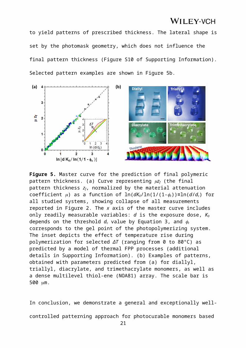
Figure S2. Photopolymerization conversion dependence on exposure time t for five systems investigated: NOA 81 (a), triallyl (b), diallyl (c), diacrylate (d) and trimethacrylate (e). These curves show the typical trend for crosslinking photopolymerization reaction, with a dependence of the conversion kinetics on the monomer reactivity. The UV light intensity was 2.8 W m-2. Reaction conversion was monitored by FT-IR spectroscopy on thin (200 μm) films, for which the crosslinking process could be considered uniform in z. Conversion was calculated monitoring the decrease of the area of the absorption band of the reactive functionality (S-H thiol groups or C=C acrylic groups centered at 2570 cm-1 and 1640 cm-1, respectively) with exposure time. A reference band at 1735 cm-1, assigned to C=O carbonyl groups, was used to calculate conversions, thus avoiding the effect of the possible volume shrinkage on the measurements. UV exposure of acrylic systems was performed in laminated conditions in order to prevent the oxygen inhibition of the reaction.

21

Figure S3. Sample thickness zf dependence on exposure time t for representative thiol-ene NOA 81 (a) and diacrylate (b) systems. Trivially, increasing the irradiation intensity I0, the exposure time required to obtain a given pattern thickness decreases. Illustrative intensity values of 2.2, 3.1 and 5.6 W m-2 are shown. Sample thickness data collapse into a single curve when reported as a function of the UV dose d, which is defined as the product of light intensity and exposure time (i.e., d≡I0×t). The logarithmic growth of zf with dose is shown in (c) for NOA 81 and (d) for diacrylate. The shrinkage induced by the photocuring reaction does not affect the logarithmic growth of the polymerizing front in the experimental conditions tested. In fact, although larger I0 induces larger shrinkage, the front kinetics remains logarithmic and unchanged with dose, even when higher intensity values are employed.

22

Figure S4. Sample thickness zf dependence on UV dose d for thiol-ene triallyl system, showing a comparison between samples cured by one continuous shot (exposure time ti) or two shots (tii=2*ti) of UV irradiation. As FPP is not an autocatalytic reaction, the polymerization front is driven forward only by the continuous flux of UV light, and samples irradiated for the same amount of time present an equivalent final thickness, independently on the number of exposures used to obtain the selected exposure time. The inset shows squared triallyl patterns obtained with one shot (left) and two shots (right) of UV irradiation, exhibiting the same thickness. This demonstrates that FPP reaction can be stopped and restarted as desired, simply by switching on and off the UV light.

Figure S5. Temperature profiles for different polymeric systems during photopolymerization: NOA 81 (a), triallyl (b), diallyl (c), diacrylate (d) and trimethacrylate (e). Temperature was measured with a thermocouple at a distance z*=1.3 mm from the illuminated surface. Dashed lines correspond to the dose required to obtain a 1.3 mm thick sample, and thus indicate the temperature at the front position. For each system, the temperature variation was measured on different samples, irradiated with increasing UV dose. For exothermic systems (i.e., triallyl, diallyl and diacrylate), the temperature increases drastically with the beginning of polymerization reaction, reaches a maximum (which does not correspond to the front position) and then decreases again, once the front has passed the thermocouple location.

23

FPP models

Minimal FPP model

The minimal FPP model[1-3] is based on physical observables and describes their spatio-

temporal evolution during photopolymerization. In particular, our model predicts the profiles

of: (i) the position of the solid/liquid front zf, which corresponds to the final pattern thickness,

and (ii) the light transmission of the material Tr. The model captures the non-linear spatio-

temporal FPP growth through a system of two coupled differential equations (Equation S1

and S2) expressing the extent of monomer-to-polymer conversion (z,t) and the light intensity

I(z,t) as a function of the distance from the illuminating surface z and the exposure time t:[1, 2]

∂ ϕ (z , t)∂ t

=K [1−ϕ ( z ,t ) ] I (z , t) (S1)

∂ I (z , t)∂z

=−μ ( z , t ) I (z ,t ) (S2)

where 1-(z,t) is the fraction of material available for conversion, and K an effective reaction

conversion rate. The transmission Tr is defined as Tr≡I(z,t)/I0, with I0≡I(z=0), and the

attenuation coefficient μ as the weighted average of the attenuation coefficients of the

unexposed monomer (μ0) and fully cured polymer (μ∞) with composition (). Often the optical

attenuation of the polymerized medium remains largely unchanged from the pure monomer (μ

≡μ0=μ∞), and the polymerization reaction is defined as photoinvariant. In this case, the system

of Equation S1 and S2 of the minimal FPP model can be solved analytically and the

conversion fraction becomes:[3]

ϕ ( z , t )=1−exp[−K I 0 exp (−μz ) t ] (S3)

The front position zf, corresponding to the solidified thickness, is then given by:

24

z f=

ln [ K I 0t

ln( 11−ϕc ) ]μ

(S4)

where c is the threshold conversion, needed to first initiate the propagation of the front.

Spatio-temporal conversion profiles of the studied monomers were experimentally measured

by FT-IR spectroscopy. Figure 4a in the main text shows that monomer-to-polymer

conversion profiles of the thiol-ene athermal system accurately follow the minimal FPP

model (Equation S3). As the incident UV light intensity I0 and the exposure time t are fixed

curing parameters, and the attenuation coefficient μ can be easily measured by light

transmission evaluation, the model has only a single fitting parameter (i.e., K). Figure 4a also

shows that for thiol-ene athermal system the value of K is nearly constant with increasing UV

dose and equal to K0, which is the photopolymerization kinetics constant at the onset of the

reaction. K0 can be calculated from the experimental critical dose and conversion values (dc

and c, respectively) by Equation S5:

K0=ln( 1

1−ϕc )dc

(S5)

Thermal FPP model

Our minimal FPP model was recently modified[4] to include thermal effects and consider the

role of heat generation during frontal photopolymerization on front propagation. In fact, as

also shown in the main text, some FPP systems polymerize via an exothermic reaction. Heat

generation and polymerization are hence coupled and reciprocally interact in a non-linear

fashion. The thermal-modified FPP model involves the introduction of an equation governing

the temperature field T=T(z,t). Moreover, it accounts for the temperature dependence of the

polymerization rate constant K, which is assumed to have an Arrhenius form:[4]

25

K (T )=K0 exp[ Ea

R ( 1T 0

− 1T )] (S6)

where Ea is the activation energy, R is the ideal gas constant, and K0 is the value of K at the

onset of the frontal photopolymerization reaction. When the UV dose transferred to the

monomer material reaches the critical value dc, K and T equal K0 and T0 respectively:

K0=K(dc), T0=T(dc).

Figure S6 shows the experimental values for thiol-ene thermal systems fitted with the

minimal model (Equation S3). This model captures the shape of the profiles, but does not take

into account the acceleration of the reaction rate due to polymerization exothermicity. For

exothermic FPP reactions, K follows the system temperature and K0 is no longer valid as

reaction constant for all exposure times.

As reported in Figure 4 of the main text, the profiles of thiol-ene thermal systems (both

triallyl and diallyl) could be instead fitted remarkably well with the thermal-modified FPP

model. Using the measured value for μ and the Arrhenius relationship between the effective

polymerization rate constant K and the temperature T, the only fitting parameter that remains

in the thermal-modified FPP model is the activation energy Ea of the polymerizing system.

Figure S6. Conversion profiles along the sample depth z for increasing UV dose d for thermal thiol-ene systems: triallyl (a) and diallyl (b). Photopolymerization was performed with a dose range of 90‒470 J m-2 for triallyl, and 120‒370 J m-2 for diallyl. Dots are experimental data, while dashed lines are minimal FPP model fits (Equation S3). The attenuation coefficient μ values used for the fitting are 0.38 mm-1 for triallyl and 0.53 mm-1 for diallyl. The value of K0 is 0.0144 and 0.0147 m2 J-1 for triallyl and diallyl, respectively. The failure of the fitting with the minimal FPP model[1, 2] demonstrates that the kinetics constant K varies during photopolymerization, following the temperature of reaction.

26

We fitted experimental profiles of acrylic systems both with the minimal[1-3] and the

thermal-modified[4] FPP models (Figure S7 and S7, respectively). However, in these cases, the

models do not accurately describe the evolution of the monomer-to-polymer conversion

during photopolymerization, as they predict a slow gradient along z, whereas, the

conversions of acrylic systems drop suddenly at a certain depth.

Figure S7. Extent of conversion dependence on sample depth z and dose d for acrylic systems: diacrylate (a) and trimethacrylate (b). Photopolymerization was conducted with a dose range of 180‒740 J m-2 for diacrylate, and 1470‒5530 J m-2 for trimethacrylate. Points are experimental data, while dashed lines are minimal FPP model fits (Equation S3). The values of the attenuation coefficient μ and of the kinetics reaction constant K0 are respectively 0.44 mm-1 and 0.0078 m2 J-1 for diacrylate, and 0.59 mm-1 and 0.0010 m2 J-1 for trimethacrylate.

Figure S8. Monomer-to-polymer conversion as a function of sample depth z and dose d for acrylate systems: diacrylate (a) and trimethacrylate (b). FPP was performed with a dose range of 180‒740 J m-2 for diacrylate, and 1470‒5530 J m-2 for trimethacrylate. Points are experimental data, while dashed lines are fits obtained using the thermal-modified FPP model.[4] The attenuation coefficient μ values employed for the fitting are 0.44 mm-1 for diacrylate and 0.59 mm-1 for trimethacrylate, which correspond to the measured values by materials transmittance analyses. The kinetics constant K varies during photopolymerization reaction (Equation S6), following the temperature of the system.

27

Experimental profiles could be fitted using both K and μ as free fitting parameters (Figure 4

in the main text). The effective reaction constant K obtained by the fitting depends on the

temperature evolution during FPP, as predicted by the thermal-modified model for exothermic

reactions; while the values of the attenuation coefficient μ are more than three times higher

than the measured values for μ0.

The experimental profiles of acrylic systems could be fitted with other theoretical

polymerization models that explicitly address the complex chemistry and kinetics of FPP,

accounting for photochemical reaction details including initiator photolysis, chain initiation,

propagation, transfer and termination. However, the increase of the level of fitting accuracy

causes an increase in the number of model parameters. As the scope of this paper is to present

a unified approach for patterning via FPP, we are more interested in considering the important

parameters for pattern transfer (e.g., curing conditions and final sample thickness), than

obtaining a precise fit for the evolution of the conversion .

Effect of temperature, light intensity and photomask dimensions on pattern thickness

Reaction exothermicity (i.e., temperature rise during FPP process) leads to an increase in the

rate of photopolymerization, and thus influences the propagation of the solidification front

and the final pattern thickness zf (Figure S9). However, numerical simulations of the thermal-

modified FPP model using typical parameter values for photopolymerizing systems[5-7] (i.e.,

Ea=10 kJ mol-1, T0=293 K) suggest that only substantial temperature rises (ΔT>50 K) will lead

to marked departures from the logarithmic behavior of zf predicted by the isothermal model.

For all systems studied in this work, the increase of temperature during polymerization

reaction can be considered small, i.e. ΔT<30 K; therefore the linearity in the master curve

reported in the main text (Figure 5) is maintained.

28

The relatively small temperature rises and activation energies for photopolymerizing systems

ensure also the planarity of the growing front. During non-isothermal frontal polymerization,

wavefronts can become unstable to a spin mode whereby a hot spot emerges on and rotates

along the perimeter of the propagating front, tracing out a helical path that imprints a similarly

helical pattern into the sample. To confirm that spin modes do not occur in our systems, we

estimat the Zeldovich number,[8] defined as:

Z=T f−T 0

T f×

Ea

R T f(S7)

and compare it to the critical value of Zc=8.4 that must be exceeded for this phenomena to

occur; Ea is the activation energy, Tf is the temperature at the front, T0 is the initial

temperature, and R is the ideal gas constant. Taking Ea=10 kJ mol-1, T0=20 °C, and Tf=45 °C,

we find that Z=0.3, which is more than one order of magnitude below the critical value of 8.4.

Figure S9. The interplay between heat generation and front propagation. Under conditions of fast thermal diffusion relative to the rate of polymerization, and limited heat exchange with the environment, the (normalized) temperature remains constant in space but changes with time/dose (a). The temperature has been normalized so that its initial and maximum values are equal to zero and one, respectively, and it has been plotted as a function of the (dimensionless) distance from the illuminating surface, µz, and the (dimensionless) dose, K0d. This normalization implies that T0 and ΔT correspond to the dimensional values of the initial temperature and the maximum temperature rise, respectively. Due Arrhenius reaction kinetics, a temperature rise leads to an increase in the rate of polymerization (b). Here, we have taken the activation energy to be equal to 10 kJ mol-1 and assumed the initial temperature is 293 K. By simulating the thermal model using the rate constant shown in panel (b) and the

29

time-varying temperature profiles with different values of ΔT in panel (c), we can ascertain how heat generation during photopolymerization influences the propagation of the solidification front (d). For temperature rises that are less than 50 K (ΔT<50 K), the dimensionless position of the solidification front, µzf, follows the logarithmic behavior predicted by the isothermal model. There is a temporary departure from this behavior for larger temperature rises (ΔT>50 K).

Photopolymerization-induced shrinkage is generally enhanced by increasing UV light

intensity. Within free radical photopolymerizing systems, thiol-ene monomers show reduced

shrinkage due to the delayed gelation caused by the mechanism of reaction via alternating

propagation and chain transfer. By contrast, (meth)acrylic systems present a higher shrinkage,

whose value depends on the monomer reactivity. For the experimental conditions used in this

work, shrinkage does not influence the universality of the reported front kinetics (Figure 5a).

Indeed, this relationship holds for a wide range of light intensities employed for FPP

patterning. Moreover, we demonstrate that the photomask geometry controls only the pattern

lateral dimensions (xy) but not its thickness (z). Patterns with the same thickness (only

defined by the material kinetics of photopolymerization and irradiation conditions) are

obtained using photomasks with different dimensions (Figure S10).

Figure S10. Effect of photomask dimensions on sample thickness. Diacrylate system was photopolymerized with a dose d=130 J m-2 with a photomask comprising squared patterns of different dimensions (a). The transparent squares of the mask have a nominal dimension of

30

the sides equals to 0.5, 0.75, 1, 1.5, 2, and 2.5 mm. The obtained patterns (b) show all the same thickness (c).

References

[1] J. T. Cabral, S. D. Hudson, C. Harrison, J. F. Douglas, Langmuir 2004, 20, 10020.

[2] J. A. Warren, J. T. Cabral, J. F. Douglas, Phys. Rev. E 2005, 72, 021801.

[3] J. T. Cabral, J. F. Douglas, Polymer 2005, 46, 4230.

[4] M. G. Hennessy, A. Vitale, J. T. Cabral, O. K. Matar, Phys. Rev. E accepted.

[5] W. D. Cook, S. Chausson, F. Chen, L. Le Pluart, C. N. Bowman, T. F. Scott, Polym.

Int. 2008, 57, 469.

[6] G. R. Tryson, A. R. Shultz, J. Polym. Sci.: Polym. Phys. 1979, 17, 2059.

[7] C. E. Hoyle, R. D. Hensel, M. B. Grubb, J. Polym. Sci.: Polym. Chem. 1984, 22, 1865.

[8] J. A. Pojman, S. Popwell, D. I. Fortenberry, V. A. Volpert, V. A. Volpert, in

Nonlinear Dynamics in Polymeric Systems, Vol. 869, American Chemical Society, 2003,

106.

31