Embed Size (px)
Citation preview

Radni materijali EIZ-a
EIZ Working Papers
.
ekonomskiinstitut,zagreb
Travanj April. 2017
Alexander Ahammer and Ivan Zilic
Br No. EIZ-WP-1701
Do Financial Incentives Alter
Physician Prescription Behavior?
Evidence from Random Patient-GP Allocations

Radni materijali EIZ-a EIZ Working Papers
EIZ-WP-1701
Do Financial Incentives Alter Physician Prescription Behavior?
Evidence from Random Patient-GP Allocations
Alexander Ahammer Department of Economics, Johannes Kepler University Linz
Altenberger Strasse 69 4040 Linz, Austria
T. +43(0)732/2468-7372 E. [email protected]
Ivan Zilic Research Assistant
The Institute of Economics, Zagreb Trg J. F. Kennedyja 7
10000 Zagreb, Croatia T. 385 1 2362238 F. 385 1 2335165
www.eizg.hr
Zagreb, April 2017

IZDAVAÈ / PUBLISHER: Ekonomski institut, Zagreb / The Institute of Economics, Zagreb Trg J. F. Kennedyja 7 10000 Zagreb Croatia T. 385 1 2362 200 F. 385 1 2335 165 E. [email protected] www.eizg.hr ZA IZDAVAÈA / FOR THE PUBLISHER: Maruška Vizek, ravnateljica / director GLAVNI UREDNIK / EDITOR: Ivan-Damir Aniæ UREDNIŠTVO / EDITORIAL BOARD: Katarina Baèiæ Tajana Barbiæ Sunèana Slijepèeviæ Paul Stubbs Marina Tkalec Iva Tomiæ Maruška Vizek IZVRŠNA UREDNICA / EXECUTIVE EDITOR: Ivana Kovaèeviæ Tiskano u 50 primjeraka Printed in 50 copies ISSN 1846-4238 e-ISSN 1847-7844 Stavovi izra�eni u radovima u ovoj seriji publikacija stavovi su autora i nu�no ne odra�avaju stavove Ekonomskog instituta, Zagreb. Radovi se objavljuju s ciljem poticanja rasprave i kritièkih komentara kojima æe se unaprijediti buduæe verzije rada. Autor(i) u potpunosti zadr�avaju autorska prava nad èlancima objavljenim u ovoj seriji publikacija. Views expressed in this Series are those of the author(s) and do not necessarily represent those of the Institute of Economics, Zagreb. Working Papers describe research in progress by the author(s) and are published in order to induce discussion and critical comments. Copyrights retained by the author(s).

Contents
Abstract 1
I. Introduction 3
I.1. Related literature and our contributions 5
II. Institutional setting 6
II.1. Country doctors and onsite pharmacies 7
II.2. Weekend prescriptions 8
III. Data 8
IV. Methodology 11
IV.1. Outcome variables 11
IV.2. Identification 12
V. Results 14
V.1. Heterogeneous effects 20
VI. Conclusions 22
VII. Bibliography 23


Do Financial Incentives Alter PhysicianPrescription Behavior?
Evidence from Random Patient-GP Allocations
Alexander Ahammer†,‡ and Ivan Zilic§,†
†Department of Economics, Johannes Kepler University Linz, Austria‡Christian Doppler Laboratory on Aging, Health, and the Labor Market, Linz, Austria
§The Institute of Economics, Zagreb, Croatia
Abstract
Do physicians respond to financial incentives? We address this question by an-alyzing the prescription behavior of physicians who are allowed to dispense drugsthemselves through onsite pharmacies. Using administrative data comprising over 16million drug prescriptions between 2008 and 2012 in Upper Austria, a naïve com-parison of raw figures reveals that self-dispensing GPs induce 33.2% higher drugexpenses than others. Our identification strategy rests on multiple pillars. First, weuse an extensive array of covariates along with multi-dimensional fixed effects whichaccount for patient and GP-level heterogeneity as well as sorting of GPs into onsitepharmacies. Second, we use a novel approach that allows us to restrict our sam-ple to randomly allocated patient-GP matches which rules out endogenous sortingas well as principal-agent bargaining over prescriptions between patients and GPs.Contrary to our descriptive analysis, we find evidence that onsite pharmacies havea small negative effect on prescriptions. Although self-dispensing GPs seem to pre-scribe slightly more expensive medication, this effect is absorbed by a much smallerlikelihood to prescribe in the first place, causing the overall effect to be negative.
Keywords: physician dispensing, drug expenses, physician agency, moral hazardJEL classification: I11, I12
1

Sazetak
Reagiraju li lijecnici na financijske poticaje? Odgovaramo na ovo pitanje anali-zom propisivanja lijekova lijecnika kojima je dopušteno prodavati lijekove u sklopuljekarne u ordinaciji. Koristeci administrativne podatke koji obuhvacaju više od 16milijuna medicinskih konzultacija izmedu 2008. i 2012. godine u Gornjoj Austriji,obicna usporedba pokazuje da postojanje ljekarne u ordinaciji rezultira 33,2% vecimtroškovima lijekova. U svrhu procjene kauzalnog efekta ljekarne u ordinaciji, koris-timo identifikacijsku strategiju koja pociva na sljedecim temeljima: prvo, koristimoširok skup kovarijata u kombinaciji s multidimenzionalnim fiksnim ucincima kojikontroliraju heterogenost pacijenata i lijecnika, kao i sortiranje lijecnika u ordinacijes ljekarnama. Drugo, koristimo novi pristup koji nam omogucuje da ogranicimo uzo-rak na nasumicno spojene parove pacijent-lijecnik što iskljucuje endogeno sortiranjepacijenata kao principala i lijecnika kao agenta. Za razliku od deskriptivne analize,nalazimo da ljekarne u ordinaciji zapravo imaju negativan utjecaj na troškove lije-kova. Iako lijecnici koji rade u ordinaciji s ljekarnom u prosjeku propisuju skupljelijekove, ukupni ucinak na troškove je negativan jer spomenuti lijecnici imaju mnogomanju vjerojatnost propisivanja bilo kojeg lijeka.
Kljucne rijeci: propisivanje lijekova, troškovi lijecenja, moralni hazardJEL klasifikacija: I11, I12
2

I. Introduction 1
Ideally, physicians are perfect agents. They diagnose and provide treatments in a waypatients would if they had perfect information. In reality, however, we observe profoundvariations in the provision of healthcare which cannot be explained by demand-side het-erogeneities. Even after adjusting for prices and patient demographics, Gottlieb et al.(2010), for example, document a $9,324 difference in per capita Medicare spending be-tween Miami, FL and Salem, OR. In general, such regional variations may result eitherfrom demand-side differences in patient health and preferences, from supply-side hetero-geneities such as physicians’ education or preferences over treatments, or from geograph-ical differences, for example, air pollution.
Most of the observed variation in healthcare utilization can be attributed to the firstchannel. Using Austrian matched patient-general practitioner (GP) data, Ahammer andSchober (2016), for example, show that patient needs and preferences explain well over90% of the variation in primary care expenses.2 While the GP explains only a smallfraction (0.12%–4.36%) relative to the variation caused by patient-side heterogeneitiesand stochastic health shocks, they find that the most lenient 10% of GPs induce roughly25% higher expenses than the average GP, which is a sizable portion. With healthcareexpenditures rising across most countries, “policy-makers are under pressure to controlpharmaceutical expenditures without adversely affecting quality of care” (Rashidian et al.2015), so understanding sources of these variations is crucial for policy making.
In this paper we focus on one specific source of variation; namely financial incentives.Under specific conditions, physicians in Austria are allowed to dispense pharmaceuticalsthemselves in the form of onsite pharmacies, which makes them entrepreneurs and agentsat the same time. Onsite pharmacies are permitted primarily for the purpose of ensuringunhindered access to medical drugs in rural areas where regular pharmacies are oftendifficult to reach. Operating an onsite pharmacy, however, allows physicians to earn amark-up on every drug they prescribe. In medical situations where no clinical guidelinesand consensus about treatments prevail, and where the marginal harm for the patient issmall, there is a clear incentive to induce demand.3
Put differently, GPs may exploit their informational advantage to prescribe medicationthe patient’s health status may not necessarily require, for the sole purpose of maximizingtheir own income. There is some causal evidence that doctors in fact do exhibit rent-
1Corresponding author: Alexander Ahammer, Department of Economics, Johannes Ke-pler University Linz, Altenberger Strasse 69, 4040 Linz, ph. +43(0)732/2468-7372, e-mail:[email protected]. We thank Gerald Pruckner, Tom Schober, Rudolf Winter-Ebmer, and sem-inar participants at the econ@JKU workshop in Schlierbach for numerous helpful discussions and valuablecomments. Eorda Sinollari provided excellent research assistance. This work has been supported by Chris-tian Doppler Laboratory “Aging, Health, and the Labor Market” and TVOJ GRANT@EIZ.
2Ahammer and Schober (2016) perform variance decompositions based on components of hierarchicalfixed effects models which contain patient-specific time-varying observables as well as both patient-leveland GP-level fixed effects. Finkelstein et al. (2016) apply a similar methodology to U.S. data with geo-graphical area as the second hierarchical level instead of GPs. They find that region-specific effects accountfor 54% of the total variation in Medicare utilization, while 47% can be explained by the patient.
3Medical situations in which clinical guidance is scarce, and the GP’s benefits of supply-inducing areidiosyncratic to the patient, are coined “gray area of medicine” by Chandra, Cutler, and Song (2012).
3

seeking behavior (e.g., Melichar 2009 or Clemens and Gottlieb 2014, see section I.1),hence we hypothesize that having an onsite pharmacy leads, ceteris paribus, to an increasein drug expenses. In order to verify this conjecture, we use administrative data from theUpper Austrian Sickness Fund (UASF) which covers around 75% of the population inUpper Austria, one of nine provinces in Austria with roughly 1.4 million inhabitants asof 2016. We have access to a total of 23,820,854 observations representing the universeof GP consultations for these insurees. Contrary to our unconditional descriptive analysiswhich reveals that self-dispensing GPs induce on average 33.2% higher per patient drugexpenses than others, first regressions reveal that doctors who run onsite pharmacies arein fact slightly less likely to prescribe medication in the first place, and induce roughlye 2.1 ($2.25 or 5.9%) lower drug expenses than their non-dispensing colleagues.
This is a surprising result, since the existing literature (Burkhard et al. 2015, Kaiserand Schmid 2016) in fact finds large positive effects of dispensing on drug prescriptions.Although our regressions so far control for physician ability and patient health status ina rigorous way, and sorting of GPs into pharmacies can be conditioned on GP-level fixedeffects, there are two other mechanisms we have to worry about: first, through a series ofconsultations, patients and GPs may develop a principal-agent relationship which allowsthe patient to bargain over drug prescriptions. In this case, the onsite pharmacy coefficientmay reflect the patient’s prescription decision rather than the GP’s, which is not what wewant to measure. Second, patients may systematically avoid GPs who operate onsitepharmacies. If this type of endogenous sorting drives our results, we expect the pharmacycoefficient to be biased towards zero.
To avoid these issues, we suggest a novel identification approach which relies on asample of randomly allocated patient-GP matches. In particular, we restrict our sampleto drugs prescribed on weekends and public holidays. On weekends and public holidays,GPs in Austria rotate to provide out-of-hours services for the purpose of ensuring basichealthcare, which is especially important in rural areas where no hospital is in close prox-imity. If a patient decides to consult a physician outside opening hours, assignment canthus be considered random, because it depends only on the community’s rotation sched-ule.4 Using this strategy to account for endogenous sorting, our estimates become evenlarger in magnitude and retain their statistical significance. We interpret this as a sign ofdefensive medicine (Chandra et al. 2012, Lucas et al. 2010): ceteris paribus, GPs seemmore reluctant to induce demand if they are not acquainted with the patient.
Overall, we find evidence that GPs who operate onsite pharmacies may not necessar-ily induce higher drug expenses than others. Although estimates suggest that GPs withonsite pharmacies prescribe slightly more expensive medication (but only if the GP is notacquainted with the patient, i.e., the patient-GP match is random), this effect is absorbedby a much smaller likelihood to prescribe something in the first place, causing the over-all effect to be negative. This is not surprising: for our sample of UASF patients, we
4To our knowledge, there is only one paper using a similar approach: Ahammer (2016) estimates labormarket effects of supply-induced sick leaves. As a robustness check, he restricts his sample to sick leavesstarting on weekends and public holidays as well. Since he does not observe the actual date of certification,however, Ahammer has to assume that it coincides with the start of the sick leave. If they are systematicallydifferent, the allocation mechanism cannot be considered random anymore. In this paper, we decided tofocus solely on drug prescriptions, since for those we know the exact date of consultation.
4

find that self-dispensing GPs earn on average an additional e 109,882.5 ($118,328.65)in revenues per year, for doing the same work as non-dispensing GPs. Thus, the finan-cial incentive to supply-induce may not be as strong as initially thought, and dispensingGPs may even prescribe more defensively due to the additional income. However, whydoes the existing literature find evidence for supply-inducement then? First, Kaiser andSchmid (2016) and Burkhard et al. (2015) may not sufficiently take into account sortingof GPs into onsite pharmacies, which would upward bias their estimated effect on drugexpenses. Second, both studies use Swiss data where in certain cantons, all physicians areallowed to dispense drugs. In our setup, only country doctors are permitted to have onsitepharmacies. In rural areas, however, competition between GPs is low, and competitionhas been shown to be associated with more aggressive prescription behavior (Ahammerand Schober 2016, Léonard et al. 2009, Scott and Shiell 1997). Lastly, onsite pharmaciestypically have a smaller variety of drugs than regular pharmacies (Pruckner and Schober2016). For pharmaceuticals they do not have in stock, incentives to overprescribe are thesame as for other GPs, which also contributes to zero effect.
I.1. Related literature and our contributions
Our paper generally belongs to the broad literature on practice styles and supply-induceddemand (see, e.g., McGuire and Pauly 1991 and Chandra et al. 2012 for overviews).In particular, we contribute to the literature on the role of financial incentives in medi-cal care. A recent example providing causal evidence is Clemens and Gottlieb (2014),who use price shocks triggered by regional Medicare consolidations in 1997 to estimatecare elasticities with respect to reimbursement rates. They find that healthcare suppliedto Medicare patients increases overproportionally with the reimbursement rate. Anothernotable example is Melichar (2009), who exploits within-physician variation in reim-bursement schemes involving different financial incentives for marginal increases in theprovision of healthcare. She finds that GPs spend less time with patients they receiveno marginal revenues for, as compared to patients whose expenses are reimbursed on afee-for-service basis. There is also experimental evidence from the field: Kouides et al.(1998), for example, document that physicians randomly selected to receive a monetarybenefit for increasing their influenza immunization rate eventually achieved a 6.9 percent-age points higher rate than physicians in the control group.
Related is also the literature on the role of onsite pharmacies in the choice of genericversus brand-name drugs in day-to-day medical care. In systems where physicians areallowed to prescribe and dispense drugs at the same time, Liu et al. (2009), Iizuka (2007,2016), and Rischatsch et al. (2013) find that profit incentives significantly affect physicianprescription behavior. Analyzing the interrelations between inpatient and outpatient pre-scription behavior, Pruckner and Schober (2016) find that GPs are less likely to adhere tothe hospital’s treatment choice if they dispense drugs themselves.
There is much less literature on the actual effect of physician self-dispensing on drugexpenses. To our knowledge, there are currently only two studies which specificallyconsider that question: Kaiser and Schmid (2016) exploit geographical variation in dis-pensing regulations across Switzerland. They empirically match physicians from cantonswhere it is permitted to operate onsite pharmacies to physicians from cantons where it
5
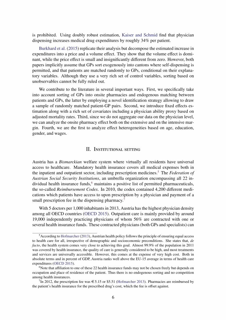
is prohibited. Using doubly robust estimation, Kaiser and Schmid find that physiciandispensing increases medical drug expenditures by roughly 34% per patient.
Burkhard et al. (2015) replicate their analysis but decompose the estimated increase inexpenditures into a price and a volume effect. They show that the volume effect is domi-nant, while the price effect is small and insignificantly different from zero. However, bothpapers implicitly assume that GPs sort exogenously into cantons where self-dispensing ispermitted, and that patients are matched randomly to GPs, conditional on their explana-tory variables. Although they use a very rich set of control variables, sorting based onunobservables cannot be fully ruled out.
We contribute to the literature in several important ways. First, we specifically takeinto account sorting of GPs into onsite pharmacies and endogenous matching betweenpatients and GPs, the latter by employing a novel identification strategy allowing to drawa sample of randomly matched patient-GP pairs. Second, we introduce fixed effects es-timation along with a rich set of covariates including a physician ability proxy based onadjusted mortality rates. Third, since we do not aggregate our data on the physician level,we can analyze the onsite pharmacy effect both on the extensive and on the intensive mar-gin. Fourth, we are the first to analyze effect heterogeneities based on age, education,gender, and wages.
II. Institutional setting
Austria has a Bismarckian welfare system where virtually all residents have universalaccess to healthcare. Mandatory health insurance covers all medical expenses both inthe inpatient and outpatient sector, including prescription medicines.5 The Federation ofAustrian Social Security Institutions, an umbrella organization encompassing all 22 in-dividual health insurance funds,6 maintains a positive list of permitted pharmaceuticals,the so-called Reimbursement Codex. In 2010, the codex contained 4,200 different medi-cations which patients have access to upon prescription by a physician and payment of asmall prescription fee in the dispensing pharmacy.7
With 5 doctors per 1,000 inhabitants in 2013, Austria has the highest physician densityamong all OECD countries (OECD 2015). Outpatient care is mainly provided by around19,000 independently practicing physicians of whom 56% are contracted with one orseveral health insurance funds. These contracted physicians (both GPs and specialists) can
5According to Hofmarcher (2013), Austrian health policy follows the principle of ensuring equal accessto health care for all, irrespective of demographic and socioeconomic preconditions. She states that, defacto, the health system comes very close to achieving this goal. Almost 99.9% of the population in 2011was covered by health insurance, the quality of care is generally considered to be high, and most treatmentsand services are universally accessible. However, this comes at the expense of very high cost. Both inabsolute terms and in percent of GDP, Austria ranks well above the EU-15 average in terms of health careexpenditures (OECD 2015).
6Note that affiliation to one of these 22 health insurance funds may not be chosen freely but depends onoccupation and place of residence of the patient. Thus there is no endogenous sorting and no competitionamong health insurances.
7In 2012, the prescription fee was e 5.15 or $5.51 (Hofmarcher 2013). Pharmacies are reimbursed bythe patient’s health insurance for the prescribed drug’s cost, which the fee is offset against.
6

be accessed free of charge and without a referral; non-contracted physicians, on the otherhand, charge a fee which will partly be reimbursed by the patient’s insurance. Patientsare not obliged to consult their GP before seeking specialist or inpatient treatment, thusgeneral practitioners formally do not serve a gatekeeping function in Austria. Although itis still common to have a family doctor, patients may also switch GPs on a regular basis.
For general practitioners, it is typically preferable to secure a contract with at leastone health insurance fund, as it guarantees a constant influx of patients and has severalbureaucratic advantages (ÖKZ 2007). Contracted positions, however, are limited. Boththe geographical distribution as well as the absolute number of contracted physicians areregulated by the Federation of Austrian Social Security Institutions. Medical profession-als that strive for a GP position thus have to pass through an application procedure wherecandidates are selected based on professional aptitude. Only contracted physicians areallowed to maintain onsite pharmacies.
II.1. Country doctors and onsite pharmacies
In a country where almost half of the population lives in predominantly rural regions(Eurostat 2013), an important pillar of outpatient medical care are country doctors (inGerman called “Landarzte”). Officially, a country doctor is a contracted physician whoeither practices in a community with up to 3,000 inhabitants, or is one of at most two con-tracted physicians in a single community (Austrian Medical Chamber 2013). Accordingto the medical chamber, roughly 40 percent of general practitioners in Austria fall withinthis category. In 2013, this amounted to 1,563 doctors being responsible for over 43% ofthe population.
More than half of these doctors, however, are expected to retire within the next tenyears. This poses an important challenge for officials and policy makers, who have longbeen lamenting about the lack of young doctors applying for vacant insurance contracts inrural areas (Austrian Medical Chamber 2013). Often living and working conditions dis-courage physicians to settle in these areas, thus the average number of applicants per coun-try doctor vacancy in Upper Austria decreased from 5 in 2001 to 1.2 in 2012. Amongstother measures, onsite pharmacies are increasingly instrumentalized by policy makers toattract physicians and counteract the expected shortage of doctors in rural areas (AustrianMedical Chamber 2013).
Onsite pharmacies require physicians to act as entrepreneurs. Typically they purchasea selection of common medications from pharmaceutical wholesalers which they dispensedirectly to the patient upon issuing a prescription. Since prices are fixed through theinsurance’s reimbursement rate, onsite pharmacies cannot compete on prices with regularpharmacies. A country doctor is permitted to operate an onsite pharmacy if (1) she iscontracted with at least one health insurance fund, (2) there is no regular pharmacy in hercommunity, and (3) the next regular pharmacy is more than six kilometers away. In 2016,the government passed a law which allows GPs to keep their onsite pharmacy even whena regular pharmacy opens within their community, as long as the pharmacy is more thanfour kilometers away. If a pharmacy opens within a radius of four kilometers around thephysician’s practice, operating an onsite pharmacy is no longer permitted.
7

II.2. Weekend prescriptions
General practitioners in Upper Austria typically work Monday to Friday. On weekendsand public holidays, each community has a rotation schedule of GPs providing out-of-hours services in order to ensure the provision of basic health care. This institution isespecially important in rural areas, where the nearest hospital is difficult to reach. Insome communities, the rotation schedule is posted on a website or in local newspapers,in others, patients have to call the emergency service (typically the Red Cross) where thedispatcher informs them about the GP on duty. If a patient decides to consult a GP on aweekend or public holiday, assignment is therefore random since it depends solely on thecommunity’s rotation schedule.
As discussed in section IV, our main estimations are based on a sample restrictedto prescriptions filed on weekends or public holidays. Indeed, this sample may also beselected if (1) patients postpone their consultation until after the weekend because theirmedical condition does not require urgent treatment, or (2) they choose to go to a hospitalinstead. As long as patients do not base their decision on whether the GP on duty hasan onsite pharmacy, neither of these selection mechanisms biases our results. In order toavoid learning effects, we use only the first match between patient and GP, so typicallythe patient will not have much information about the doctor.
III. Data
The main source of data for our empirical analysis is the Upper Austrian Sickness Fund(UASF), which gathers detailed information on health care utilization in both the inpatientand outpatient sector for roughly one million insurees. As described in section II, theseinsurees correspond to about three quarters of the Upper Austrian population, composedof private as well as public sector workers, retirees, and unemployed people. We augmentthe data with information on patient education and wages from the Austrian Social Secu-rity Database (Zweimüller et al. 2009) as well as additional demographic information onphysicians from the Upper Austrian Medical Chamber.
For our analysis we draw a sample comprising the universe of medical drug pre-scriptions issued by general practitioners between 2008 and 2012.8 In total, we observe16,341,428 prescriptions issued by 632 GPs to 1,135,893 patients — on average, thisamounts to roughly 14 prescriptions per patient over the entire period. Additionally, weadd all available consultations that did not result in a drug prescription to our data, whichallows us to analyze the effect of financial incentives at the extensive margin, i.e., theoverall probability of receiving medication when a GP is consulted. Our primary cri-terion for including a prescription is whether it is issued by a general practitioner. Forself-dispensing GPs, we also include drugs that are dispensed at a regular pharmacy (i.e.,not sold at the onsite pharmacy).9 In total, this leaves us with a sample of 23,820,854
8Unfortunately, our data does not allow us to analyze outcomes other than medical drug prescriptions,since we do not have an exact date of consultation (which we need to define our weekend sample) fornon-drug health services. Kaiser and Schmid (2016) find that drug and non-drug expenditures are comple-mentary goods for self-dispensing physicians.
9This could, for example, be the case for certain uncommon medications (such as cancer drugs) the GP
8

consultations.
Our main regressions are based on a subset of these data, namely drug prescriptions is-sued on weekends or public holidays (for convenience we call this the “weekend sample”henceforth). If a patient visited the same GP multiple times on weekends or holidays, wekeep only the first consultation in order to avoid learning effects. For reasons discussedin section IV.2, we are primarily interested in weekend and public holiday prescriptionsbecause they provide more reliable estimates than the full sample. Thus, we do not in-clude drug prescriptions by specialists, since they typically do not provide out-of-hoursservices on weekends.
Summary statistics are provided in Table 1, where we provide first and second mo-ments of our most important variables for the full sample, the weekend subsample, anda sample of “changers”. The latter is simply a subset of the full sample comprising thelargest connected set of consultations filed by GPs who opened or closed an onsite phar-macy at least once during our observation period. Because we include GP fixed effects inour estimations, these are in fact the observations which ultimately identify our results.Note that the means of the changer sample are remarkably similar to those obtained fromthe full sample, thus fixed effects estimates should be representative as well.
Our four outcome variables are discussed extensively in section IV. At the exten-sive margin, we estimate the effect of onsite pharmacies on a binary variable indicatingwhether at least one unit of medication is prescribed during the consultation (i.e., drugexpenses are positive), and overall drug expenses of the consultation, including also zerosfor consultations where no drug was prescribed. At the intensive margin, we look at drugexpenses per unit and at the number of units prescribed, both conditional on receiving atleast one unit of medication. On weekends and public holidays, in general it seems thatslightly less medication is prescribed.
Our treatment indicator is a binary variable indicating whether the consulted GP op-erates an onsite pharmacy, and zero otherwise. Around 30% of all GPs operate an onsitepharmacy; this corresponds roughly to the official numbers cited in section II.1. In theweekend sample, the fraction of GPs with onsite pharmacies is higher, which makes sensegiven that weekend consultations are used more by people living in rural areas, where alsoonsite pharmacies are much more common than in densely populated areas. For the GP,we also have information on gender and age: it seems that GPs in Upper Austria are pre-dominantly men aged 50 or older. Again, these numbers coincide with the official figurespresented in section II.1.
At the patient level, we control for age, wages, and health proxies — these are time-varying variables, and their means reflect mostly what we expect a priori. Additionally,we have information on gender, education, and migratory status. Overall, patients aremore likely to be male, around 50% are between 50 and 80 years of age, and their high-est educational degree is most likely apprenticeship training. Health proxies are the sumof drug expenses in the year prior to the consultation (“medication history”) and the ag-gregate number of days spent in hospital the year prior to the consultation (“hospital his-
may not have in stock at her onsite pharmacy. In general, we expect onsite pharmacies to have a smallervariety of medications than regular pharmacies, which is also a result in Pruckner and Schober (2016).
9

Table 1 — Descriptive statistics.
Full sample Weekend sampleaDiff.b Changersc
Mean Std. dev. Mean Std. dev. Mean Std. dev.
OutcomesPositive expenses 0.686 0.464 0.541 0.498 0.145 0.688 0.463Total expenses (in EUR) 35.642 147.779 24.191 156.145 11.451 35.963 201.439Units of medication 2.010 3.899 1.362 3.046 0.648 1.967 3.804
GP characteristicsOnsite pharmacy 0.299 0.458 0.347 0.476 −0.048 0.746 0.435Female 0.122 0.327 0.111 0.314 0.011 0.539 0.498Age
Under 35 0.002 0.039 0.001 0.035 0.0003 0 035 to 40 0.010 0.102 0.009 0.094 0.001 0.079 0.27040 to 45 0.041 0.197 0.032 0.176 0.009 0.243 0.42945 to 50 0.107 0.309 0.088 0.283 0.019 0.311 0.46350 to 55 0.256 0.436 0.233 0.423 0.023 0.212 0.40955 to 60 0.342 0.474 0.360 0.480 −0.018 0.138 0.34560 to 65 0.201 0.401 0.227 0.419 −0.026 0.017 0.128Over 65 0.042 0.200 0.051 0.219 −0.009 0 0
Adjusted mortality 1.000 0.003 1.000 0.003 0.0001 1.000 0.003Patient characteristics
Female 0.564 0.496 0.536 0.499 0.029 0.571 0.495Age
Under 20 0.098 0.297 0.141 0.348 −0.043 0.119 0.32420 to 30 0.076 0.265 0.099 0.299 −0.024 0.076 0.26530 to 40 0.087 0.281 0.109 0.312 −0.023 0.088 0.28440 to 50 0.130 0.336 0.155 0.362 −0.026 0.127 0.33350 to 60 0.159 0.366 0.167 0.373 −0.008 0.155 0.36260 to 70 0.183 0.387 0.144 0.351 0.039 0.177 0.38270 to 80 0.162 0.368 0.116 0.320 0.046 0.167 0.373Over 80 0.106 0.308 0.069 0.253 0.038 0.091 0.287
EducationCompulsory 0.063 0.243 0.073 0.260 −0.010 0.061 0.240Apprenticeship 0.156 0.363 0.198 0.399 −0.042 0.162 0.368High school 0.117 0.322 0.152 0.359 −0.034 0.118 0.323University 0.034 0.182 0.040 0.196 −0.006 0.030 0.170Missing 0.629 0.483 0.537 0.499 0.092 0.629 0.483
Daily wage (in EUR) 27.872 43.745 36.373 46.925 −8.501 27.393 42.628Migrant 0.166 0.372 0.160 0.366 0.006 0.168 0.374Medication historyd 159.829 494.278 122.481 448.909 37.349 154.987 457.232Hospital historye 0.599 3.812 0.463 3.303 0.136 0.562 3.599
ATC medication codeMissing 0.033 0.178 0.039 0.194 −0.006 0.025 0.155Alimentary tract and metabolism 0.108 0.310 0.079 0.270 0.029 0.115 0.319Blood and blood forming organs 0.015 0.122 0.010 0.101 0.005 0.016 0.125Cardiovascular system 0.199 0.399 0.136 0.342 0.063 0.206 0.405Dermatologicals 0.015 0.120 0.012 0.111 0.002 0.014 0.116Genito-urinary system 0.016 0.124 0.010 0.102 0.005 0.017 0.129Systemic hormonal preparations 0.018 0.131 0.014 0.119 0.003 0.018 0.132Antiinfectives for systemic use 0.059 0.236 0.067 0.250 −0.008 0.066 0.249Antineoplastic and imm. agents 0.006 0.078 0.005 0.069 0.001 0.007 0.083Musculo-skeletal system 0.065 0.247 0.051 0.220 0.014 0.066 0.248Nervous system 0.102 0.302 0.073 0.261 0.028 0.088 0.283Antiparasitic products 0.0004 0.020 0.0003 0.018 0.0001 0.0004 0.021Respiratory system 0.044 0.205 0.038 0.190 0.006 0.041 0.198Sensory organs 0.006 0.079 0.005 0.070 0.001 0.008 0.089Various 0.001 0.028 0.001 0.026 0.0001 0.001 0.035
Sample size 23,820,854 2,089,438 — 484,415
Notes: This table presents summary statistics for our sample of consultations.a Sample is restricted to medications prescribed on weekends or public holidays.b Difference in means between the full sample and the weekend sample.c Sample of patients receiving medication from GPs that changed their onsite pharmacy status at least once between 2008 and 2012.d Medication history is the aggregate amount of drug expenses one year prior to the consultation.e Hospital history is the aggregate number of days spent in hospital one year prior to the consultation.
10

tory”). On top of that, we include a full set of region-specific controls in our estimations.10
These are especially important because we want to pick up as much location-specific het-erogeneity as possible.
Finally, we use the Anatomical Therapeutic Chemical (ATC) classification system tocontrol for the type of medication prescribed. Unfortunately, we do not have informationon diagnoses, thus the ATC code serves as a proxy for the medical condition the patientsuffers from. Around 40% of all drugs prescribed fall within one of these categories:alimentary tract and metabolism (e.g., laxatives, antidiarrhoeals, antidiabetics, vitamins,or dietary minerals), cardiovascular system (e.g., beta blockers, cardiac stimulants, orantiarrhythmics), or nervous system (e.g., analgesics, antidepressants, anti-ADHD agents,etc.), with cardiac therapy drugs being the most common.
IV. Methodology
We estimate the following fixed effects model:
yijt = ϑ · 1{ospijt} + Xijtβ′ + Witγ
′ + Z jtδ′ + Miϕ
′ + η j + τt + εijt (1)
where yijt is medical care received by individual i = 1, . . . ,N provided by GP j = 1, . . . , Jat time t = 1, . . . ,Ti, thus subscript ijt uniquely identifies a consultation. The treatmentindicator 1{ospijt} ∈ {0, 1} equals unity if GP j providing medical care to individual imaintains an onsite pharmacy at time t, and zero otherwise — our main coefficient ofinterest is therefore ϑ.
Additionally, the vector Xijt contains consultation-specific control variables such asthe first letter of the prescribed drug’s ATC classification system code, the vector Wit
comprises time-variant patient-level controls such as age, wage, and a full set of commu-nity fixed effects, Z jt captures time-variant GP-level control variables such as age and ameasure of physician ability (adjusted GP-specific mortality rates, see section IV.2 for adetailed description), and Mi contains patient-level time-invariant control variables (e.g.,gender, migratory status, and education). Finally, we include a full set of GP-level fixedeffects η j as well as year and month fixed effects τt.
IV.1. Outcome variables
Let expijt be the sum of prices of all drugs prescribed in consultation ijt in euros, and letvolijt be the number of units of drugs prescribed (typically packages). Then, our vector ofoutcome variables yijt consists of
(1) “positive expenses” 1{expijt > 0} ∈ {0, 1}, an indicator variable which equals unitywhen patient i receives some medication from GP j during the consultation at timet, and zero if the patient does not receive any medication,
10We build geographical clusters based on the first three out of four figures of the patient’s zip code —these correspond roughly to larger communities.
11
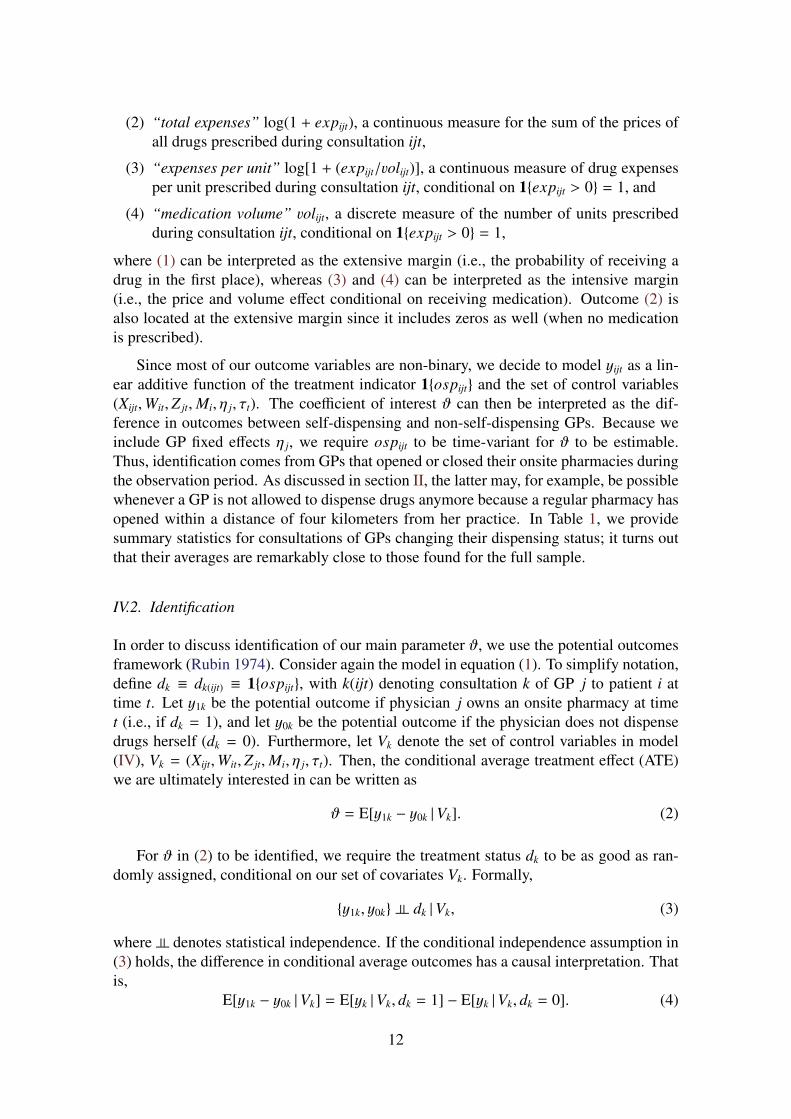
(2) “total expenses” log(1 + expijt), a continuous measure for the sum of the prices ofall drugs prescribed during consultation ijt,
(3) “expenses per unit” log[1 + (expijt/volijt)], a continuous measure of drug expensesper unit prescribed during consultation ijt, conditional on 1{expijt > 0} = 1, and
(4) “medication volume” volijt, a discrete measure of the number of units prescribedduring consultation ijt, conditional on 1{expijt > 0} = 1,
where (1) can be interpreted as the extensive margin (i.e., the probability of receiving adrug in the first place), whereas (3) and (4) can be interpreted as the intensive margin(i.e., the price and volume effect conditional on receiving medication). Outcome (2) isalso located at the extensive margin since it includes zeros as well (when no medicationis prescribed).
Since most of our outcome variables are non-binary, we decide to model yijt as a lin-ear additive function of the treatment indicator 1{ospijt} and the set of control variables(Xijt,Wit,Z jt,Mi, η j, τt). The coefficient of interest ϑ can then be interpreted as the dif-ference in outcomes between self-dispensing and non-self-dispensing GPs. Because weinclude GP fixed effects η j, we require ospijt to be time-variant for ϑ to be estimable.Thus, identification comes from GPs that opened or closed their onsite pharmacies duringthe observation period. As discussed in section II, the latter may, for example, be possiblewhenever a GP is not allowed to dispense drugs anymore because a regular pharmacy hasopened within a distance of four kilometers from her practice. In Table 1, we providesummary statistics for consultations of GPs changing their dispensing status; it turns outthat their averages are remarkably close to those found for the full sample.
IV.2. Identification
In order to discuss identification of our main parameter ϑ, we use the potential outcomesframework (Rubin 1974). Consider again the model in equation (1). To simplify notation,define dk ≡ dk(ijt) ≡ 1{ospijt}, with k(ijt) denoting consultation k of GP j to patient i attime t. Let y1k be the potential outcome if physician j owns an onsite pharmacy at timet (i.e., if dk = 1), and let y0k be the potential outcome if the physician does not dispensedrugs herself (dk = 0). Furthermore, let Vk denote the set of control variables in model(IV), Vk = (Xijt,Wit,Z jt,Mi, η j, τt). Then, the conditional average treatment effect (ATE)we are ultimately interested in can be written as
ϑ = E[y1k − y0k |Vk]. (2)
For ϑ in (2) to be identified, we require the treatment status dk to be as good as ran-domly assigned, conditional on our set of covariates Vk. Formally,
{y1k, y0k} |= dk |Vk, (3)
where |= denotes statistical independence. If the conditional independence assumption in(3) holds, the difference in conditional average outcomes has a causal interpretation. Thatis,
E[y1k − y0k |Vk] = E[yk |Vk, dk = 1] − E[yk |Vk, dk = 0]. (4)
12

Due to the extensive array of control variables, we are confident that most systematicdifferences in patients and GPs which may be correlated with dk are accounted for in ourregressions. However, there are two main threats to identification which we will discussin more detail here, both related to self-selection. First, GPs may self-select into onsitepharmacies. Our main remedy to deal with that issue is to include GP fixed effects inmodel (1), arguing that the unobserved propensity to self-select into dispensing is likelya time-invariant personality trait, or at least a characteristic that does not change overtime. Additionally, we follow Biørn and Godager (2010) and Markussen et al. (2012)and construct adjusted mortality rates as a proxy for physician ability, which is likely alsoa determinant of self-selection into dispensing and potentially time-variant (e.g., throughfurther education). We proceed as follows: first, define a family doctor j for every patient iin the UASF data, and build a yearly panel for i = 1, . . . ,N and t = 1, . . . ,T . Second,perform the following regression:
Pr[1{deadit} = 1] = π1 · ageit + π2 · 1{ f emalei} + Citψ′ + ξit (5)
where 1{deadit} ∈ {0, 1} is a binary variable indicating whether patient i died in year t andCit is a vector of community dummies. Third, average the predicted values obtained fromestimating model (5) via OLS over all patients of GP j: Let Pj be the set of patients ofGP j, and let Pj be the cardinality of Pj, then
Λ j =1
PjT
Pj∑i=1 | i∈Pj
T∑t=1
Pr[1{deadit}] (6)
is the adjusted mortality rate for GP j.
Controlling for physician ability along with age and GP-level fixed effects, we believethat most unobserved factors determining endogenous sorting of GPs into self-dispensingare accounted for in our model. A different sorting mechanism, however, may also im-pede identification, namely endogenous matching of patients to certain GPs. Again, wesuppose that most factors driving these sorting decisions are already controlled for in ourregressions (most importantly physician ability) — however, our results may still be bi-ased if there are unobserved determinants we do not catch. Therefore, we restrict oursample to consultations on weekends and public holidays.
On weekends and public holidays, GP practices in Upper Austria are typically closed.As discussed in section II.2, however, each community has a schedule of GPs rotating toprovide out-of-hours services in order to ensure medical care in emergency cases. Sincepatients do not know which GP is on duty if they get sick on a weekend, the allocationbetween patient and GP is as good as random. In section II.2, we briefly discuss two caseswhere this sample may still be selected on unobservables: (1) if the patient postpones hervisit until after the weekend, and (2) if the patient decides to go to a hospital instead.As long as the patient does not base her decision on whether the GP on duty operates anonsite pharmacy, these cases will not affect identification in our framework.11 Since thepatient does not have any information about the GP on duty (which we ensure by keeping
11Note that, even if the patient considers the dispensing status of the matched GP when deciding whetherto consult the GP, postpone her visit or go to a hospital, our estimates would be lower bounds of the actualeffect.
13

Table 2 — Average per patient per year drug expenses for GPs with and without onsite pharmacies.
Onsite pharmacy
No Yes Difference(1) (2) (3)
Non-adjusted drug expenses (in EUR) 50.75 67.62 33.2%Adjusted drug expenses (in EUR) 16.57 18.65 12.6%
Notes: This table gives the difference in average per patient per year drug ex-penses of GPs who do not maintain an onsite pharmacy (“No”) and those whodo (“Yes”). The adjusted difference is based on residuals from regressing drugexpenses on a third-order polynomial in age and a female dummy.
only the first patient-GP match if there are multiple), we believe that this is a plausibleassumption.
Another appealing feature of using only weekend prescriptions is that it eliminates cer-tain principal-agent dynamics which may have evolved between patient and GP. Througha series of consultations, patients may develop a relationship with their GPs which al-lows them to bargain over drug prescriptions. Because we only use random patient-GPmatches, such dynamics do not distort identification either. In section V, we report re-sults both for the full sample as well as for the weekend sample since comparing theseestimates may provide insight about the effects of patient and GP self-selection on drugprescriptions. Generally, we expect estimated onsite pharmacy effects to be upwards bi-ased if there is endogenous sorting of GPs into onsite pharmacies, and to be downwardsbiased if patients systematically avoid GPs with onsite pharmacies.
V. Results
In Table 2, we present average yearly per patient drug expenses, both for GPs operat-ing an onsite pharmacy and for those who do not dispense drugs themselves. For non-dispensing GPs, non-adjusted drug expenses are based on prescriptions issued by the GPand dispensed at a regular pharmacy. For self-dispensing GPs, in contrast, we consideronly prescriptions that are dispensed directly at the onsite pharmacy, disregarding drugswhich are dispensed at a regular pharmacy.12
Average drug expenses of self-dispensing GPs are e 16.87 ($18.17) or 33.2% higherthan the drug expenses induced by other GPs. Since we only consider drugs dispensedand billed directly by the GP, e 67.62 ($72.82) can be interpreted as the average yearlyrevenue generated through the onsite pharmacy. Self-dispensing GPs have on average1,625 patients; their total average revenue per year is thus e 109,882.5 ($118,328.63),which they earn on top of reimbursements paid by the health insurance for other medical
12As discussed in section III, our data also comprises drugs prescribed by a self-dispensing GP butdispensed by a regular pharmacy instead of the GP herself. The reason is that we are interested in howfinancial incentives affect prescription behavior overall, irrespective of whether the GP in fact sells the drugherself in the end or issues a prescription for a regular pharmacy.
14

Table 3 — Estimation results for full sample.
Extensive margin Intensive margin
Positive Total Expenses Medicationexpenses expenses per unit volume
(1) (2) (3) (4)
Onsite pharmacy −0.022∗∗∗ −0.059∗∗ 0.011 0.014(0.008) (0.028) (0.009) (0.021)
Patient is female 0.013∗∗∗ −0.020∗∗∗ −0.070∗∗∗ 0.014(0.001) (0.004) (0.002) (0.010)
Patient drug historya 0.0001∗∗∗ 0.001∗∗∗ 0.0002∗∗∗ 0.001∗∗∗
(0.00001) (0.0001) (0.00002) (0.0001)
Patient hospital historyb 0.002∗∗∗ 0.019∗∗∗ 0.004∗∗∗ 0.061∗∗∗
(0.0001) (0.001) (0.0003) (0.002)
Patient wage −0.017∗∗∗ −0.054∗∗∗ 0.016∗∗∗ −0.055∗∗∗
(0.001) (0.003) (0.001) (0.005)
Patient is migrant 0.023∗∗∗ 0.025∗∗∗ −0.057∗∗∗ 0.009(0.002) (0.006) (0.004) (0.011)
GP adjusted mortality 0.206∗ 0.665∗ −0.141 2.332∗∗
(0.114) (0.383) (0.154) (1.115)
GP fixed effects Yes Yes Yes YesYear and month Yes Yes Yes YesATC codes — — Yes YesPatient education and age Yes Yes Yes YesGP age Yes Yes Yes YesCommunity fixed effects Yes Yes Yes Yes
Observations 23,820,854 23,820,854 16,341,428 16,341,428Adjusted R2 0.188 0.236 0.176 0.072
Notes: In this table we present results from estimating equation (1) on the full sample of general practitionerconsultations. Every column represents an individual regression estimated by OLS: in column (1), theoutcome is 1{expijt > 0}; in column (2), the outcome is log(1 + expijt); in column (3), the outcome islog[1 + (expijt/volijt)]; and in column (4), the outcome is volijt. Heteroskedasticity-robust and community-level clustered standard errors are given in parentheses below coefficients; stars indicate significance levels:* p < 0.1, ** p < 0.05, *** p < 0.01.a Medication history is the aggregate amount of drug expenses one year prior to the consultation.b Hospital history is the aggregate number of days spent in hospital one year prior to the consultation.
services. The main purpose of this paper is to verify how much of this difference can beascribed to the possibility of self-dispensing, and how much is caused by other factorssuch as patient health or endogenous sorting.
In Table 3, we take a closer look at the determinants of individual drug prescriptions.Before we turn to our main analysis based on a sample of randomly allocated patient-GPmatches, we run our estimations on the universe of drug prescriptions in order to gaina more comprehensive picture. For a detailed discussion of our four outcome variableswe refer the reader to section IV.1 — in general, columns (1) and (2) should captureeffects at the extensive margin (i.e., the overall probability of receiving medication), whilecolumns (3) and (4) consider the intensive margin (i.e., given that the patient receives
15

Table 4 — Estimation results for sample of weekend and public holiday prescriptions, extensivemargin.
Positive expenses Total expenses
(1) (2) (3) (4) (5) (6)
Onsite pharmacy −0.128∗∗∗ −0.125∗∗∗ −0.123∗∗∗ −0.419∗∗ −0.391∗∗ −0.389∗∗
(0.049) (0.046) (0.045) (0.192) (0.175) (0.175)
Patient is female 0.023∗∗∗ 0.022∗∗∗ 0.010∗∗ 0.009∗
(0.001) (0.001) (0.005) (0.005)
Patient drug historya 0.0001∗∗∗ 0.0001∗∗∗ 0.001∗∗∗ 0.001∗∗∗
(0.00001) (0.00001) (0.0001) (0.0001)
Patient hospital historya 0.002∗∗∗ 0.002∗∗∗ 0.016∗∗∗ 0.016∗∗∗
(0.0002) (0.0002) (0.001) (0.001)
Patient wage −0.020∗∗∗ −0.020∗∗∗ −0.050∗∗∗ −0.050∗∗∗
(0.001) (0.001) (0.003) (0.003)
Patient is migrant 0.007∗∗ 0.007∗∗ −0.004 −0.004(0.003) (0.003) (0.010) (0.010)
GP adjusted mortality 0.309 −0.937(0.642) (2.022)
GP fixed effects Yes Yes Yes Yes Yes YesYear and month Yes Yes Yes Yes Yes YesATC codes Yes Yes Yes Yes Yes YesPatient education and age Yes Yes Yes YesGP age Yes YesCommunity fixed effects Yes Yes
Observations 2,089,438 2,089,438 2,089,438 1,130,723 1,130,723 1,130,723Adjusted R2 0.348 0.395 0.396 0.138 0.228 0.229
Notes: In this table we present results from estimating equation (1) on the sample of weekend and publicholiday GP consultations. Every column represents an individual regression estimated by OLS: in columns(1), (2), and (3), the outcome is 1{expijt > 0}; in columns (4), (5), and (6), the outcome is log(1 + expijt).Heteroskedasticity-robust and community-level clustered standard errors are given in parentheses belowcoefficients; stars indicate significance levels: * p < 0.1, ** p < 0.05, *** p < 0.01.a Medication history is the aggregate amount of drug expenses one year prior to the consultation.b Hospital history is the aggregate number of days spent in hospital one year prior to the consultation.
medication, what determines its expenses and volume). Inference is based on analyticalheteroskedasticity-robust and community-level clustered standard errors.
In column (1) we consider the overall probability of receiving medication as an out-come. In contrast to our descriptive analysis, we find that consulting a GP who has anonsite pharmacy in fact decreases the likelihood of receiving medication by 2.2 percent-age points, which corresponds to 3.3% of the sample mean. In column (2), we find asimilar effect: overall expenses decrease by 5.9% — in terms of the sample mean, thiscorresponds to a reduction from e 35.64 ($38.38) to e 33.54 ($36.12). Thus, we findrather small yet statistically significant effects at the extensive margin.
Columns (3) and (4) are only observed conditional on receiving at least one unit ofmedication. For both expenses per unit and the number of units, we find small positive
16

Table 5 — Estimation results for sample of weekend and public holiday prescriptions, intensivemargin.
Expenses per unit Medication volume
(1) (2) (3) (4) (5) (6)
Onsite pharmacy 0.031 0.038∗∗ 0.038∗∗ 0.033 0.032 0.044(0.019) (0.019) (0.019) (0.125) (0.113) (0.118)
Patient is female −0.074∗∗∗ −0.074∗∗∗ −0.072∗∗∗ −0.070∗∗∗
(0.003) (0.003) (0.014) (0.014)
Patient drug historya 0.0002∗∗∗ 0.0002∗∗∗ 0.001∗∗∗ 0.001∗∗∗
(0.00003) (0.00003) (0.0001) (0.0001)
Patient hospital historyb 0.003∗∗∗ 0.003∗∗∗ 0.052∗∗∗ 0.052∗∗∗
(0.0004) (0.0004) (0.003) (0.003)
Patient wage 0.021∗∗∗ 0.021∗∗∗ −0.048∗∗∗ −0.047∗∗∗
(0.001) (0.001) (0.004) (0.004)
Patient is migrant −0.045∗∗∗ −0.044∗∗∗ −0.009 −0.014(0.004) (0.004) (0.013) (0.013)
GP adjusted mortality −0.102 −2.736(0.378) (2.488)
GP fixed effects Yes Yes Yes Yes Yes YesYear and month Yes Yes Yes Yes Yes YesATC codes Yes Yes Yes Yes Yes YesPatient education and age Yes Yes Yes YesGP age Yes YesCommunity fixed effects Yes Yes
Observations 1,130,723 1,130,723 1,130,723 1,130,723 1,130,723 1,130,723Adjusted R2 0.166 0.215 0.217 0.019 0.066 0.066
Notes: In this table we present results from estimating equation (1) on the sample of weekend and publicholiday GP consultations. Every column represents an individual regression estimated by OLS: in columns(1), (2), and (3), the outcome is 1{expijt > 0}; in columns (4), (5), and (6), the outcome is log(1 + expijt).Heteroskedasticity-robust and community-level clustered standard errors are given in parentheses belowcoefficients; stars indicate significance levels: * p < 0.1, ** p < 0.05, *** p < 0.01.a Medication history is the aggregate amount of drug expenses one year prior to the consultation.b Hospital history is the aggregate number of days spent in hospital one year prior to the consultation.
yet statistically insignificant effects. Thus, it seems that GPs with onsite pharmacies areslightly less likely to prescribe medication in the first place which leads also to a small de-crease in overall expenses. Once medication is prescribed, we do not find any statisticallysignificant differences between self-dispensing and non-self-dispensing GPs.
A priori, we would expect the onsite pharmacy effect to be positive. Similar to resultsfrom the available empirical literature, our descriptive analysis also clearly points towardssubstantial excess prescription of dispensing GPs, which would be consistent with the no-tion of physicians simply being profit-maximizing individuals who respond to financialincentives. How can we rationalize this small negative effect? We do not necessarilyneglect the possibility that GPs are profit-maximizing individuals, yet we conjecture thatGPs may not necessarily face a strong enough incentive to overprescribe, because poten-
17

tial benefits do not exceed the cost associated with the risk of harming the patient. Keep inmind that onsite pharmacies yield an average e 109,882.5 ($118,328.63) in revenues forthe same work other GPs earn nothing for. Thus, the additional income generated throughonsite pharmacies may allow the GPs to prescribe more defensively, along the lines ofLucas et al. (2010). Furthermore, onsite pharmacies generally maintain a smaller varietyof drugs, and for drugs they do not have in stock, dispensing GPs have the same incentiveto induce demand as non-self-dispensing GPs. This could also explain a zero effect.
Why does the existing literature find signs of supply-inducement then? First, Kaiserand Schmid (2016) and Burkhard et al. (2015) both assume that sorting of GPs into onsitepharmacies is exogenous. This may cause an upwards bias to their results which we in turnpick up with our GP fixed effects and the physician ability measure. Second, Kaiser andSchmid (2016) and Burkhard et al. (2015) both use Swiss data where in certain cantonsall doctors are allowed to dispense drugs, whereas in Austria only country doctors arepermitted to do so. Country doctors may differ from others in their propensity to inducedemand, which could explain the diverging results. We also know that in rural areascompetition between GPs is small, and competition is typically associated with moregenerous prescription behavior (Ahammer and Schober 2016, Léonard et al. 2009, Scottand Shiell 1997). A lack of competition may explain why our observed doctors inducelower drug expenses in general.
As discussed in section IV, we are worried that endogenous sorting between patientsand GPs may partly drive the effects estimated on the full sample of GP consultations. Wetherefore turn to the sample of weekend and public holiday prescriptions (see section IV.2for details) where matches between patients and GPs are randomized. Estimation resultscan be found in Tables 4 and 5, where Table 4 considers effects at the extensive marginwhile Table 5 gives effects at the intensive margin. In both tables we present three differentspecifications for each outcome: in the first column we show the crude onsite pharmacyeffect only controlling for GP fixed effects, time fixed effects, and the ATC code of themedical drug. In the second column we extend the set of covariates by patient-levelobservables — in particular, gender, age, migratory status, education, health proxies, andwages. In the third column we complete the model and also include time-varying GP levelobservables (i.e., age and ability proxy) as well as community fixed effects.
On the extensive margin we still find a negative and statistically significant effect ofconsulting a self-dispensing GP on drug expenses. The probability of receiving medica-tion in the first place decreases by at least 12.3 percentage points — this is a rather largeeffect, corresponding to a reduction from 54.1% to 41.8% in terms of the sample mean.Since, conversely, the likelihood of having zero medical expenses increases by 12.3 per-centage points, overall expenses also decrease by a large 38.9%. This amounts to a reduc-tion from e 24.2 ($26.1) to e 14.8 ($15.9). These results suggest that the negative effectof having an onsite pharmacy is much more pronounced outside opening hours whenthe patient-GP match is random. Potentially, this could be a sign of defensive medicine(Chandra et al. 2012, Lucas et al. 2010) if GPs encounter patients whom they do notknow, or conversely, of prescribing relatively more aggressively as soon as a relationshipbetween principal and agent has been built and developed.
On the intensive margin (Table 5), we find a positive effect for drug expenses per unit:
18

Figure 1 — Heterogeneous effects for different patient age groups, weekend sample, extensivemargin.
-1.2
-1.0
-0.8
-0.6
-0.4
-0.2
0.0
(0,20] (20,30] (30,40] (40,50] (50,60] (60,70] (70,80] 80+Patient age groups
On-
site
phar
mac
y ef
fect
Positive expenses Total expenses
Notes: This graph depicts estimated onsite pharmacy coefficients and 95% confidence intervals from sep-arate regressions where the sample is stratified on different patient age groups and the outcome variablesare “positive expenses” and “total expenses” (see section IV.1 for a detailed description). The underlyingsample consists of weekend and public holiday consultations.
If at least one unit of medication is prescribed, self-dispensing GPs induce 3.8% higherexpenses per unit. Again, we do not find any effect on medication volume. For patientsthat are unknown to the GP, self-dispensing therefore reduces the likelihood of receivingmedication. If medication is prescribed, however, it is marginally more expensive if theGP is self-dispensing. Since this effect is offset by the smaller probability of prescribingin the first place, the overall effect of onsite pharmacies on drug expenses is negative.
In terms of our other covariates, coefficients largely have their expected sign. Fe-males are more likely to receive medication, yet at lower cost. Sicker patients (indicatedthrough positive coefficients on the drug and hospital) receive more and relatively ex-pensive drugs, migrants receive more but cheaper drugs, and low-ability GPs prescribemore, ceteris paribus. Interestingly, higher wages seem to have a negative effect on theextensive margin, which may also be a result of lower information asymmetry betweenprincipal and agent if we expect wages to be positively correlated with ability. Note alsothat our estimated onsite pharmacy coefficient is fairly stable across specifications, indi-cating a small correlation with other patient and GP-level observables.
19

Figure 2 — Heterogeneous effects for different GP age groups, weekend sample, extensive margin.
-0.9
-0.6
-0.3
0.0
0.3
45 and less (45,60] more than 60GP age groups
On-
site
phar
mac
y ef
fect
Positive expenses Total expenses
Notes: This graph depicts estimated onsite pharmacy coefficients and 95% confidence intervals from sep-arate regressions where the sample is stratified on different GP age groups and the outcome variables are“positive expenses” and “total expenses” (see section IV.1 for a detailed description). The underlying sam-ple consists of weekend and public holiday consultations.
V.1. Heterogeneous effects
In Figures 1, 2, and 3, we depict estimates of the onsite pharmacy coefficients for differ-ent subsamples of the population. We restrict our analysis to outcomes on the extensivemargin in the weekend sample. In all estimations we use the most comprehensive specifi-cation from columns (3) and (6) in Table 4. Figure 1 suggests that the older the patient is,the more reluctant a GP who operates an onsite pharmacy is to prescribe medication. Thepatient-age gradient is nonlinear — while the magnitude of the effect for both measuresof the extensive margin is fairly stable up to 40 years of age, the effect increases dramat-ically for subsequent age groups, until it again stabilizes at the 70 year mark. Figure 2depicts effect heterogeneities for different GP age groups. We find that the negative effecton both outcomes at the extensive margin are mainly driven by mid-aged (45 to 60 yearsold) GPs, while both younger and older ones do not change their prescription behaviorsignificantly if they have onsite pharmacies. For old GPs (above 60 years of age), we finda small positive effect, which is statistically insignificant nonetheless. Figure 3 shows thatthe onsite pharmacy effect increases with decreasing patient education, i.e., dispensingGPs prescribe more defensively when the patient is uneducated.
Finally, Table 6 presents heterogeneous results based on patient gender and wage(where high wage is defined as above median wage, and low wage is defined as belowmedian wage) as well as GP gender for all four outcomes considered before. Interest-
20

Figure 3 — Heterogeneous effects for different patient education groups, weekend sample, exten-sive margin.
-0.6
-0.4
-0.2
0.0
Compulsary Apprenticeship High school UniversityPatient education
On-
site
phar
mac
y ef
fect
Positive expenses Total expenses
Notes: This graph depicts estimated onsite pharmacy coefficients and 95% confidence intervals from sep-arate regressions where the sample is stratified on different patient education groups and the outcomevariables are “positive expenses” and “total expenses” (see section IV.1 for a detailed description). Theunderlying sample consists of weekend and public holiday consultations.
ingly, our estimated onsite pharmacy effects seem to be driven mostly by female doctors.For male doctors effects on the extensive margin are negative as well, yet smaller in mag-nitude and statistically insignificant. We do, however, observe a positive and borderlinesignificant effect on number of units prescribed for males. In terms of patient gender wefind almost equal effects throughout, although they generally seem to be slightly strongerfor females. In terms of patient wage, effects are stronger for those earning below median.
21
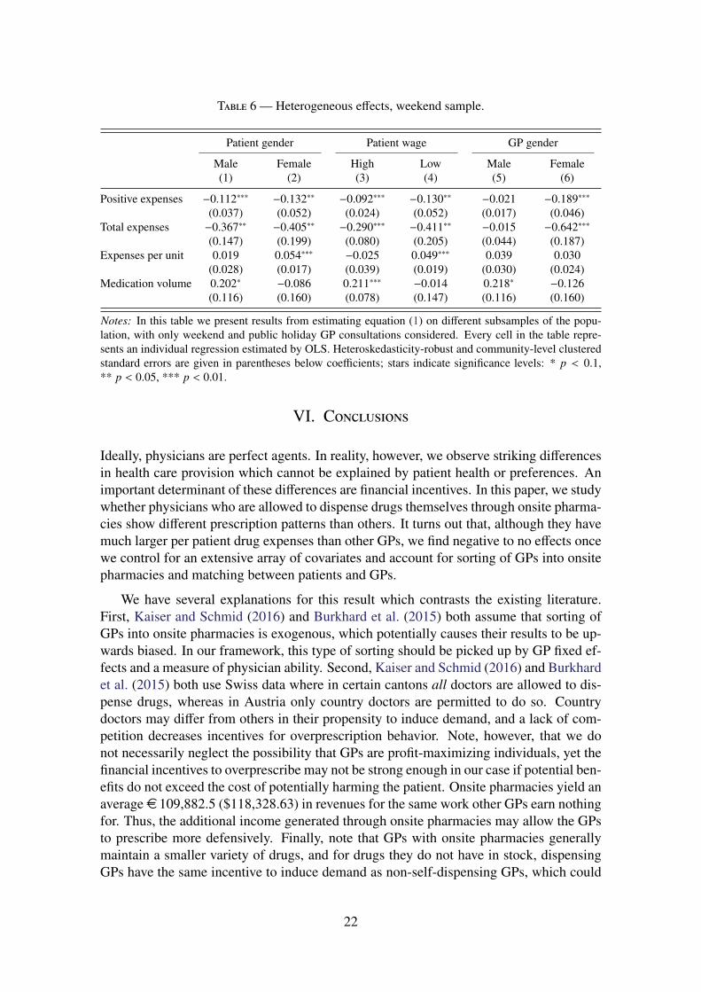
Table 6 — Heterogeneous effects, weekend sample.
Patient gender Patient wage GP gender
Male Female High Low Male Female(1) (2) (3) (4) (5) (6)
Positive expenses −0.112∗∗∗ −0.132∗∗ −0.092∗∗∗ −0.130∗∗ −0.021 −0.189∗∗∗
(0.037) (0.052) (0.024) (0.052) (0.017) (0.046)Total expenses −0.367∗∗ −0.405∗∗ −0.290∗∗∗ −0.411∗∗ −0.015 −0.642∗∗∗
(0.147) (0.199) (0.080) (0.205) (0.044) (0.187)Expenses per unit 0.019 0.054∗∗∗ −0.025 0.049∗∗∗ 0.039 0.030
(0.028) (0.017) (0.039) (0.019) (0.030) (0.024)Medication volume 0.202∗ −0.086 0.211∗∗∗ −0.014 0.218∗ −0.126
(0.116) (0.160) (0.078) (0.147) (0.116) (0.160)
Notes: In this table we present results from estimating equation (1) on different subsamples of the popu-lation, with only weekend and public holiday GP consultations considered. Every cell in the table repre-sents an individual regression estimated by OLS. Heteroskedasticity-robust and community-level clusteredstandard errors are given in parentheses below coefficients; stars indicate significance levels: * p < 0.1,** p < 0.05, *** p < 0.01.
VI. Conclusions
Ideally, physicians are perfect agents. In reality, however, we observe striking differencesin health care provision which cannot be explained by patient health or preferences. Animportant determinant of these differences are financial incentives. In this paper, we studywhether physicians who are allowed to dispense drugs themselves through onsite pharma-cies show different prescription patterns than others. It turns out that, although they havemuch larger per patient drug expenses than other GPs, we find negative to no effects oncewe control for an extensive array of covariates and account for sorting of GPs into onsitepharmacies and matching between patients and GPs.
We have several explanations for this result which contrasts the existing literature.First, Kaiser and Schmid (2016) and Burkhard et al. (2015) both assume that sorting ofGPs into onsite pharmacies is exogenous, which potentially causes their results to be up-wards biased. In our framework, this type of sorting should be picked up by GP fixed ef-fects and a measure of physician ability. Second, Kaiser and Schmid (2016) and Burkhardet al. (2015) both use Swiss data where in certain cantons all doctors are allowed to dis-pense drugs, whereas in Austria only country doctors are permitted to do so. Countrydoctors may differ from others in their propensity to induce demand, and a lack of com-petition decreases incentives for overprescription behavior. Note, however, that we donot necessarily neglect the possibility that GPs are profit-maximizing individuals, yet thefinancial incentives to overprescribe may not be strong enough in our case if potential ben-efits do not exceed the cost of potentially harming the patient. Onsite pharmacies yield anaverage e 109,882.5 ($118,328.63) in revenues for the same work other GPs earn nothingfor. Thus, the additional income generated through onsite pharmacies may allow the GPsto prescribe more defensively. Finally, note that GPs with onsite pharmacies generallymaintain a smaller variety of drugs, and for drugs they do not have in stock, dispensingGPs have the same incentive to induce demand as non-self-dispensing GPs, which could
22

also explain a zero effect.
The target of future research clearly should be to obtain further evidence on the rela-tionship between onsite pharmacies and prescription behavior for other countries. Also,our empirical setup does not allow us to look at outcomes other than drug prescriptions;analyzing effects on non-drug services along the lines of Kaiser and Schmid (2016) woulddefinitely add to our understanding of onsite pharmacies.
VII. Bibliography
A. Ahammer. Physicians Affect Patients’ Employment Outcomes Through Deciding on SickLeave Durations. Working Paper 1605, Johannes Kepler University Linz, Department of Eco-nomics, 2016.
A. Ahammer and T. Schober. Explaining Variations in Health Care Expenditures – What is theRole of Practice Styles? Unpublished manuscript, Johannes Kepler University Linz, Depart-ment of Economics, 2016. Presentation slides including methodological details and main resultsare available on ResearchGate: http://dx.doi.org/10.13140/RG.2.1.2303.4645.
Austrian Medical Chamber. Landmedizin in Österreich – Aktuelle Situation und Zukunft. Press re-lease, 2013. Transcript available under http://www.aerztekammer.at/archiv/-/asset_publisher/h4S0/content/id/2210468, accessed Wednesday 22nd March, 2017.
E. Biørn and G. Godager. Does Quality Influence Choice of General Practitioner? An Analysisof Matched Doctor-Patient Panel Data. Economic Modelling, 27(4):842–853, 2010. ISSN0264-9993. doi: http://dx.doi.org/10.1016/j.econmod.2009.10.016. Special Issue on HealthEconometrics.
D. Burkhard, C. Schmid, and K. Wüthrich. Financial Incentives and Physician Prescription Be-havior: Evidence From Dispensing Regulations. Discussion Paper 15–11, University of Bern,2015.
A. Chandra, D. Cutler, and Z. Song. Who Ordered That? The Economics of Treatment Choicesin Medical Care. In M. V. Pauly, T. E. McGuire, and P. E. Barros, editors, Handbook of HealthEconomics, volume 2. North Holland, 2012.
J. Clemens and J. Gottlieb. Do Physicians’ Financial Incentives Affect Medical Treatment andPatient Health? American Economic Review, 104(4):1320–1349, 2014. ISSN 00028282. doi:10.1257/aer.104.4.1320.
Eurostat. Eurostat Regional Yearbook 2013, chapter 15, ‘Focus on Rural Development’, pages237–275. European Comission, 2013.
A. Finkelstein, M. Gentzkow, and H. Williams. Sources of Geographic Variation in Health Care:Evidence From Patient Migration. Quarterly Journal of Economics, 131(4):1681–1726, 2016.doi: 10.1093/qje/qjw023.
D. J. Gottlieb, W. Zhou, Y. Song, K. G. Andrews, J. S. Skinner, and J. M. Sutherland. Prices Don’tDrive Regional Medicare Spending Variations. Health Affairs, 29(3):537–543, 2010.
M. M. Hofmarcher. Austria: Health System Review 2013. In W. Quentin, editor, Health Systemsin Transition, volume 15. European Observatory on Health Systems and Policies, 2013.
T. Iizuka. Experts’ Agency Problems: Evidence from the Prescription Drug Market in Japan.RAND Journal of Economics, 38(3):844–862, 2007. ISSN 07416261.
23

T. Iizuka. Physician Agency and Adoption of Generic Pharmaceutical. American Economic Re-view, 102(6):2826–2858, 2016.
B. Kaiser and C. Schmid. Does Physician Dispensing Increase Drug Expenditures? EmpiricalEvidence from Switzerland. Health Economics, 25(1):71–90, 2016. ISSN 1099-1050. doi:10.1002/hec.3124.
R. W. Kouides, N. M. Bennett, B. Lewis, J. D. Cappuccio, W. H. Barker, F. M. LaForce, et al.Performance-based Physician Reimbursement and Influenza Immunization Rates in the Elderly.American Journal of Preventive Medicine, 14(2):89–95, 1998.
C. Léonard, S. Stordeur, and D. Roberfroid. Association Between Physician Density and HealthCare Consumption: A Systematic Review of the Evidence. Health Policy, 91(2):121–134, 2009.ISSN 0168-8510. doi: http://dx.doi.org/10.1016/j.healthpol.2008.11.013.
Y. M. Liu, Y. H. K. Yang, and C. R. Hsieh. Financial Incentives and Physicians’ PrescriptionDecisions on the Choice Between Brand-name and Generic Drugs: Evidence from Taiwan.Journal of Health Economics, 28(2):341–349, 2009. ISSN 01676296. doi: 10.1016/j.jhealeco.2008.10.009.
F. L. Lucas, B. E. Sirovich, P. M. Gallagher, A. E. Siewers, and D. E. Wennberg. Variation in Car-diologists’ Propensity to Test and Treat. Circulation: Cardiovascular Quality and Outcomes, 3(3):253–260, 2010. ISSN 1941-7705. doi: 10.1161/CIRCOUTCOMES.108.840009.
S. Markussen, A. Mykletun, and K. Røed. The Case for Presenteeism – Evidence From Norway’sSickness Insurance Program. Journal of Public Economics, 96(11-12):959–972, 2012. ISSN00472727. doi: 10.1016/j.jpubeco.2012.08.008.
T. G. McGuire and M. V. Pauly. Physician response to fee changes with multiple payers. Journalof Health Economics, 10(4):385–410, 1991. ISSN 01676296. doi: 10.1016/0167-6296(91)90022-F.
L. Melichar. The Effect of Reimbursement on Medical Decision Making: Do Physicians AlterTreatment in Response to a Managed Care Incentive? Journal of Health Economics, 28(4):902–907, 2009. ISSN 01676296. doi: 10.1016/j.jhealeco.2009.03.004.
OECD. Health at a Glance 2015. OECD Indicators. OECD Publishing, 2015.
ÖKZ. Vom Jungmediziner zum Kassenarzt. In Das österreichische Gesundheitswesen – DieZeitschrift für das österreichische Gesundheitssystem, volume 48, pages 7–10. Schaffler Verlag,2007.
G. J. Pruckner and T. Schober. Hospitals and the Generic Versus Brand-name Prescription Deci-sion in the Outpatient Sector. Working Paper 1611, Johannes Kepler University Linz, Depart-ment of Economics, 2016.
A. Rashidian, A.-H. Omidvari, Y. Vali, H. Sturm, and A. D. Oxman. Pharmaceutical Policies:Effects of Financial Incentives for Prescribers. Cochrane Database of Systematic Reviews, 8(CD006731), 2015.
M. Rischatsch, M. Trottmann, and P. Zweifel. Generic Substitution, Financial Interests, and Im-perfect Agency. International Journal of Health Care Finance and Economics, 13(2):115–138,2013. ISSN 13896563. doi: 10.1007/s10754-013-9126-5.
D. B. Rubin. Estimating Causal Effects of Treatments in Randomized and Nonrandomized Studies.Journal of Educational Psychology, 66(5):688–701, 1974.
A. Scott and A. Shiell. Analysing the Effect of Competition on General Practitioners’ BehaviourUsing a Multilevel Modelling Framework. Health Economics, 6(6):577–588, 1997. ISSN
24
1099-1050. doi: 10.1002/(SICI)1099-1050(199711)6:6<577::AID-HEC291>3.0.CO;2-Y.
J. Zweimüller, R. Winter-Ebmer, R. Lalive, A. Kuhn, J.-P. Wuellrich, O. Ruf, and S. Büchi. Aus-trian Social Security Database. Working Paper 0903, NRN: The Austrian Center for LaborEconomics and the Analysis of the Welfare State, 2009.
25

9 771846 423001
I S S N 1 8 4 6 - 4 2 3 8