Does Unusual News Forecast Market Stress?

Harry Mamaysky and Paul Glasserman∗

Initial version: July 2015. Current version: August 2016

Abstract

We find that an increase in the “unusualness” of news with negative sentiment pre-

dicts an increase in stock market volatility. Similarly, unusual positive news forecasts

lower volatility. Our analysis is based on more than 360,000 articles on 50 large finan-

cial companies, mostly banks and insurers, published in 1996–2014. We find that the

interaction between measures of unusualness and sentiment forecasts volatility at both the

company-specific and aggregate level. These effects persist for several months. The ob-

served behavior of volatility in our analysis can be explained by attention constraints on

investors.

∗Columbia Business School and Office of Financial Research (OFR). This paper was produced while Paul

Glasserman was a consultant to the OFR. We acknowledge the excellent research assistance of Il Doo Lee. We

thank Paul Tetlock, Geert Bekaert, Kent Daniel, and seminar participants at the Summer 2015 Consortium for

Systemic Risk Analytics conference, Columbia, the Office of Financial Research, the High Frequency Finance

and Analytics conference at the Stevens Institute, the IAQF/Thalesians seminar, the Imperial College London

Quantitative Finance Seminar, the Princeton Quant Trading Conference, the Columbia-Bloomberg Machine

Learning in Finance Workshop, and BNY Mellon’s Machine Learning Day for valuable comments. We thank

the Thomson Reuters Corp. for graciously providing the data that was used in this study. We use the Natural

Language Toolkit in Python for all text processing applications in the paper. For empirical analysis we use the

R programming language for statistical computing.

1 Introduction

Can the content of news articles forecast market stress and, if so, what type of content is

predictive? Several studies have documented that news sentiment forecasts market returns. We

find that a measure of “unusualness” of news text combined with sentiment forecasts stress,

which we proxy by stock market volatility. The effects we find play out over months, whereas

in most prior work the stock market’s response to news articles dissipates in a few days.

The link between sentiment expressed in public documents and stock market returns has

received a great deal of attention. At an aggregate level, Tetlock (2007) finds that negative

sentiment in the news depresses returns; Tetlock, Saar-Tsechansky, and Macskassy (2008), using

company-specific news stories and responses, show this relationship also holds at the individual

firm level. Garcia (2008) finds that the influence of news sentiment is concentrated in recessions.

Loughran and McDonald (2011) and Jegadeesh and Wu (2013) apply sentiment analysis to 10-K

filings. Da, Engelberg, and Gao (2014) measure sentiment in Internet search terms. Manela

and Moreira (2015) find that a news-based measure of uncertainty forecasts returns. Our focus

differs from prior work because we seek to forecast market stress rather than the direction of

the market. We apply new tools to this analysis, going beyond sentiment word counts.

The importance of unusualness is illustrated by the following two phrases, both of which

appeared in news articles from September 2008:

“the collapse of Lehman”

“cut its price target”

Both phrases contain one negative word and would therefore contribute equally to an overall

measure of negative sentiment in a standard word-counting analysis. But we recognize the first

phrase as much more unusual than the second, relative to earlier news stories. This difference

can be quantified by taking into account the frequency of occurrence of the phrases in prior

months. As this simple example suggests, we find that sentiment is important, but it becomes

more informative when interacted with our measure of unusualness.

Research in finance and economics has commonly measured sentiment through what is known

in the natural language processing literature as a bag-of-words approach: an article is classified as

having positive or negative sentiment based on the frequency of positive or negative connotation

words that it contains. The papers cited above are examples of this approach. As the example

above indicates, this approach misses important information: the unusualness of the first phrase

2

lies not in its use of “collapse” or “Lehman” but in their juxtaposition. We therefore measure

unusualness of consecutive word phrases rather than individual words.

Our analysis uses all news articles in the Thomson Reuters Corp. database between January

1996 and December 2014 that mention any of the top 50 global banks, insurance, and real estate

firms by market capitalization as of February 2015. After some cleaning of the data, this leaves

us with 367,331 articles, for an average of 1,611 per month. We calculate measures of sentiment

and unusualness from these news stories and study their ability to forecast realized or implied

volatility at the company-specific and aggregate levels.

The consistent picture that emerges from this analysis is that the interaction of unusual-

ness with sentiment yields the best predictor of future stock market volatility among the news

measures we study.1 Importantly, our analysis shows that news is not absorbed by the market

instantaneously. We also find that the information in news articles relevant for future company-

specific volatility is better reflected in firm-level option prices than macro-relevant information

is reflected in the prices of S&P 500 options.

We first run forecasting regressions of company-specific implied volatility on company-specific

news measures and evaluate results in the cross section. Our interacted measure of unusual

negative news, ENTSENT NEG, provides a statistically and economically significant predictor

of volatility at lags of up to six months. Negative sentiment and unusualness are also significant

separately, but much less so. Across companies, our interacted measure increases R2 by an

average of 0.22, relative to a baseline control model, more than any of the other news measures

we consider.

We then introduce controls for lagged values of implied and realized volatilities and negative

returns, all of which are known to be relevant predictors of volatility; see, for example, Poon and

Granger (2003) and Bekaert and Hoerova (2014). We include these controls in panel regressions

of company-specific volatility measures on company-specific news measures. Even with the

inclusion of the controls, our interacted measures of sentiment (both positive and negative)

and unusualness remain economically and statistically significant at lags of up to two months,

with positive measures forecasting a decrease in volatility and negative measures forecasting an

increase. These results indicate that the information in our news measures is not fully reflected

in contemporaneous option prices.

1Loughran and McDonald (2011) similarly find that sentiment provides a stronger signal when they putgreater weight on less frequently occurring words, but the empirical word weights in Jegadeesh and Wu (2013)are only weakly related to word frequency.

3

For our aggregate analysis we extract aggregate measures of unusualness and sentiment from

our full set of news articles. We estimate vector autoregressions, taking as state variables the

VIX, realized volatility on the S&P 500, and several aggregate news measures. We examine

interactions among the variables through impulse response functions. A shock to either nega-

tive sentiment or our interacted variable ENTSENT NEG produces a statistically significant

increase in both implied and realized volatility over several months. Once again, the effect is

strongest for our interacted measure of unusual negative news. The response of implied and

realized volatility to an impulse in ENTSENT NEG (or negative sentiment, ENTSENT ) is

hump-shaped, peaking at around four months, and remaining significant even after ten months.

This pattern suggests that the information in these news variables is absorbed slowly. We

find similar results (but forecasting a decrease in volatility) for the interaction between positive

sentiment and unusualness, though the effects are stronger for negative news than positive news.

In most prior work that finds a predictive signal in the text of public documents, the in-

formation is incorporated into prices within a few days.2 In contrast, we find that, even after

controlling for known predictors of future volatility, news measures forecast volatility at lags

as long as ten months at the macro level, and two months at the firm level. Furthermore, we

show that company specific news is more fully incorporated into firm level option prices than

aggregate news is incorporated into the price of S&P 500 option – even though both types of

news are useful for forecasting future volatility. These are two of the most intriguing features of

our results, so we suggest potential explanations.

The delayed response of volatility to news can be partly explained by a simple difference

between forecasting volatility and forecasting returns. A predictable increase in realized volatil-

ity in the future — associated, for example, with a scheduled announcement or event — need

not lead to a near-term increase in realized volatility. It should increase implied volatility, but

arbitraging a predictable rise in volatility is more difficult than profiting from a predictable stock

return: the term structure of implied volatility is typically upward sloping, the roll yield on VIX

futures is typically negative, and implied volatility is typically higher than realized volatility,

so trades based on options, futures or variance swaps need to overcome these hurdles. These

arguments are fully consistent with market efficiency.

But this cannot be the entire story. Why does aggregate volatility initially underreact to

news? Furthermore, why do individual firm options better reflect firm level news than S&P 500

options reflect aggregated news flow? One unifying explanation for these phenomena is that

2An exception is Heston and Sinha (2014). By aggregating news weekly, they find evidence of predictabilityover a three-month horizon.

4

market participants have only a limited ability to process the information in tens of thousands

of news articles. A given market participant is better able to to process news about a specific

company than news about the macro economy simply because there is much less company-

specific news.

Rational inattention offers a possible framework for these patterns. Several studies have

found evidence that the limits of human attention affect market prices; see, for example, the

survey of Daniel, Hirshleifer, and Teoh (2004). Models of rational inattention, as developed

in Sims (2003, 2015), attach a cost or constraint on information processing capacity: investors

cannot (or prefer not to) spend all their time analyzing the price implications of all available

information. We interpret the cost or constraint on information processing broadly. It includes

the fact that people cannot read thousands of news articles per day (and having a computer do

the analysis involves some investment); but it also reflects limits on the contracts investors can

write to hedge market stress, given imperfect information on unobservable macro state variables.

The capacity constraint faced by investors forces them to specialize – even among profession-

als, many investors may focus on a narrow set of stocks or industries and may overlook informa-

tion that becomes relevant only when aggregated over many stocks. Indeed, Jung and Shiller

(2005) review empirical evidence supporting what they call Samuelson’s dictum, that the stock

market is micro efficient but macro inefficient. The allocation of attention between indiosyn-

cratic and aggregate information by capacity constrained agents is examined in the models of

Mackowiak and Wiederholt (2009b), Peng and Xiong (2006), Kacperczyk, Van Nieuwerburgh,

and Veldkamp (2016), and Glasserman and Mamaysky (2016). Mackowiak and Wiederholt

(2009b) (with regard to firms) and Glasserman and Mamaysky (2016) (with regard to investors)

find that economic agents favor micro over macro information.3 The equilibrium effect of this,

as shown in Glasserman and Mamaysky (2016), is to make prices more informationally efficient

with regard to micro than macro information. Thus attention constrained investors are one

explanation for why individual firm option prices better reflect company specific information

than S&P 500 options reflect aggregate information.

Furthermore, capacity constrained investors also need to allocate attention across different

time horizons. Dellavigna and Pollet (2007) find that demographic information with long-term

implications is poorly reflected in market prices. A related effect may apply in our setting:

investors may anticipate the possibility of elevated volatility in the future yet not start trading

options to act on that anticipation until their view is confirmed by the arrival of more data.

3Peng and Xiong (2006) reach the opposite conclusion when looking at the information choice of a represen-ative investor.

5

Beyond this qualitative link to rational inattention we develop a precise connection. First, we

argue that although investors would like to hedge aggregate risk, information constraints make

it impossible to write contracts directly tied to unobservable macro state variables. Instead

investors can only design a hedging instrument that tracks these unobservable macro state

variables as closely as possible (in a sense made precise in Section 6). We interpret the VIX as

an example of just such an imperfect hedging instrument. Next we solve for the price of this

imperfect hedge in a formulation consistent with rational inattention, meaning that investors

evaluate the conditional expectation of future cash flows based on imperfect information about

the past. Building on work of Sims (2003, 2015) and Mackowiak and Wiederholt (2009b),

we show that when investors face binding information-processing constraints, the response of

the VIX to an impulse in the macro state variable is hump-shaped rather than monotonically

decaying. This provides a coherent theoretical explanation for the underreaction of aggregate

volatility that we find in the data.

Because the effects we find in the data play out over months, the signals we extract from news

articles are potentially useful for monitoring purposes. Along these lines, Baker, Bloom, and

Davis (2013) develop an index of economic policy uncertainty based (partially) on newspaper

articles. Indicators of systemic risk (see Bisias et al. 2012) are generally based on market prices

or lagged economic data; incorporating news analysis offers a potential direction for improved

monitoring of stress to the financial system. From a methodological perspective, our work

applies two ideas from the field of natural language processing to text analysis in finance. As

already noted, we measure the “unusualness” of language, and we do this through a measure

of entropy in word counts. Also, we take consecutive strings of words (called n-grams) rather

than individual words as our basic unit of analysis. In particular, we calculate the unusualness

(entropy) of consecutive four-word sequences. These ideas are developed in greater detail in

Jurafsky and Martin (2009). See Das (2014)and Loughran and McDonald (2016) for an overview

of text analysis with applications in finance.

The rest of this paper is organized as follows. Section 2 introduces the methodology we

use, and Section 3 discusses the empirical implementation. Section 4 presents results based on

company-specific volatility, and Section 5 examines aggregative volatility. Section 6 discusses

possible explanations of our results and develops the connection with rational inattention. Sec-

tion 7 concludes. An appendix presents evidence that the results in Sections 4 and 5 are robust

across different subperiods of the data, and are not unduly influenced by the financial crisis of

2007-2009.

6

2 Methodology

2.1 Unusualness of language

A text is unusual if it has low probability, so measuring unusualness requires a model of the

probability of language. This problem has been studied in the natural language processing

literature on word prediction. Jurafsky and Martin (2009), a very thorough reference for the

techniques we employ in this paper, gives the following example: What word is likely to follow

the phrase please turn your homework ...? Possibly it could be in or over, but a word like the

is very unlikely. A reasonable language model should give a value for

P (in|please turn your homework)

that is relatively high, and a value for

P (the|please turn your homework)

that is close to zero. One way to estimate these probabilities is to count the number of times

that in or the have followed the phrase please turn your homework in a large body of relevant

text.

An n-gram is a sequence of n words or, more precisely, n tokens.4 Models that compute these

types of probabilities are called n-gram models (in the above example, n = 5) because they give

the probability of seeing the nth word conditional on the first n− 1 words.

To use an example from our dataset, up until October 2011, which is around the start of the

European sovereign debt crisis, the phrase negative outlook on had appeared 688 times, and had

always been followed by the word any. In October 2011, we observe in our sample 13 occurrences

of the phrase negative outlook on France. We would like our language model to consider this

phrase unusual given the observed history.

Consider an N -word sentence w1 . . . wN . We can write its probability as

P (w1 . . . wN) = P (w1)P (w2|w1)P (w3|w1w2) · · ·P (wN |w1w2 . . . wN−1). (1)

4For example, we treat “chief executive officer” as a single token. When we refer to “words” in the followingdiscussion, we always mean tokens.

7

N-gram models are used in this context to approximate conditional probabilities of the form

P (wk|w1 . . . wk−1) when k is so large (practically speaking, for k ≥ 6) that it becomes difficult

to provide a meaningful estimate of the conditional probabilities for most words. In the case of

an n-gram model, we assume that

P (wk|w1 . . . wk−1) = P (wk|wk−(n−1) . . . wk−1),

which allows us to approximate the probability in (1) as

P (w1 . . . wN) ≈N∏k=n

P (wk|wk−n+1 . . . wk−1). (2)

In (2), we have dropped first n− 1 terms from (1).

A text or corpus is a collection of sentences.5 Let us refer to the text whose probability (or

unusualness) we are trying to determine as the evaluation text. Since the true text model is not

known, the probabilities in (2) will have to be estimated from a training corpus, which is usually

very large relative to the evaluation text.

Assuming sentences are independent, the probability of an evaluation text is given by the

product of the probabilities of its constituent sentences. Say the evaluation text consists of I

distinct n-grams {ωi1 ωi2 ωi3 ωi4} each occuring ci times. From (2), we see that the evaluation

text probability can be written as

Peval =I∏i=1

P (ωin|ωi1 · · ·ωin−1)ci . (3)

The probabilities P (ωin|ωi1 · · ·ωin−1) in (3) are estimated from the training corpus. For a 4-

gram {ω1 ω2 ω3 ω4}, the empirical probability of ωi4 conditional on ω1 ω2 ω3 will be denoted by

mi, and is given by

mi =c({ω1 ω2 ω3 ω4})c({ω1 ω2 ω3})

(4)

5This has the effect of only counting as an n-gram a contiguous n-word phrase that does not cross a sentenceboundary. Another option, as suggested by Jurafsky and Martin (2009, p.89), is to use a start and end ofsentence token as part of the language vocabulary and then allow n-grams to lie in adjoining sentences. Thiswould greatly increase the number of n-grams in our study, and due to data sparsity we did not pursue thisoption.

8

where c(·) is the count of the given 3- or 4-gram in the training corpus.6

Taking logs in (3) and dividing by the total number of n-grams in the evaluation text,

w1 . . . wN , we obtain the per word, negative log probability of this text:

Heval ≡ − 1∑k ck

logP (w1 . . . wN) = − 1∑k ck

I∑i=1

ci logmi

= −I∑i=1

pi logmi, (5)

where pi is the fraction of all n-grams represented by the ith n-gram.

The evaluation text is unusual if it has low probability Peval, relative to the training corpus.

Equation (5) shows that, in an n-gram model, the evaluation text is unusual if there are n-grams

that occur frequently in the evaluation text (as measured by pi) but rarely in the training corpus

(as measured by mi).

The quantity in (5) is called the cross-entropy of the model probabilities mi with respect

to the observed probabilities pi (see Jurafsky and Martin (2009) equation (4.62)). We refer to

Heval simply as the entropy of the evaluation text. Based on this definition, unusual texts will

have high entropy.

Lists of n-grams

The definition of entropy in (5) can apply to an arbitrary list of n-grams, as opposed to all the

n-grams in a text, as long as we know the count for each n-gram in the list. For example, we may

want to consider the list of n-grams that include the word “France,” or the list of all n-grams

appearing in articles about banks. For a list j of n-grams, we denote by {cj1(t), . . . , cjI(t)} the

counts of the number of times each n-gram appears in month t. For an n-gram i that does not

appear in list j in month t, cji (t) = 0.

Given these counts, for each n-gram i we can calculate

pji (t) =cji (t)∑i cji (t)

,

6We will address in Section 3.3 how to handle the situation that the n-gram {wk−n+1 . . . wk} was not observedin the training corpus.

9

which is i’s fraction of the total count of n-grams in list j. Given a list of n-grams in month t,

the entropy of that list will be defined as

Hj(t) ≡ −∑i

pji (t) logmi(t), (6)

which is a generalization of (5). As in (4), the mi are conditional probabilities estimated from

a training corpus. We write mi(t) to emphasize that these are estimated from news articles

published prior to month t. As explained in Section 3.3, we use a rolling window to calculate

mi(t).

Alternative Measures

In their analysis of 10-Ks, Loughran and McDonald (2011) find that sentiment measures are

more informative when individual words are weighted based on their frequency of occurrence.

They use what is known in the text analysis literature as a tf-idf scheme because it accounts

for term frequency and inverse document frequency. The weight assigned to each word in each

document depends on the number of occurrences of the word in the document and the fraction

of documents that contain the word. A word in a document gets greater weight if it occurs

frequently in that document and rarely in other documents. This approach is less well suited to

our setting because we do not analyze individual documents and because our unit of analysis is

the n-gram rather than the individual word. The entropy measure allows a more direct measure

of the unusualness of an entire body of text in one period relative to another.

Tetlock (2011) uses measures of similarity between news articles as proxies for staleness

of news. His primary measure is the ratio of the number of words that two articles have in

common to the number of distinct words occurring in the two articles combined. Although

similar measures could potentially be used in our setting, Tetlock’s (2011) approach seems

better suited to comparing pairs of articles than to comparing large bodies of text.

2.2 Sentiment

The traditional approach for evaluating sentiment has been to calculate the fraction of words

in a given document that have negative or positive connotations. To do so, researchers rely

on dictionaries that classify words into different sentiment categories. Tetlock (2007) and Tet-

lock, Saar-Tsechansky, and Macskassy (2008) use the Harvard IV-4 psychosocial dictionary.

10

Recent evidence (Loughran and McDonald (2011) and Heston and Sinha (2014)) shows that

the Laughran-McDonald7 word lists do a better job of sentiment categorization in a financial

context than the Harvard dictionary. We use the Laughran-McDonald dictionary in our work.

Because our core unit of analysis is the n-gram, we take a slightly different approach than

the traditional literature. Rather than counting the number of positive or negative words in a

given article, we classify n-grams as being either positive or negative. An n-gram is classified as

positive (negative) if it contains at least one positive (negative) word and no negative (positive)

words. We can then measure the tone of (subsets of) news stories by looking at the fraction of

n-grams they contain which are classified as either positive or negative.

3 Empirical implementation

Our dataset consists of Thomson Reuters news articles about the top 50 global banks, insurance,

and real estate firms by U.S. dollar market capitalization as of February 2015.8 Almost 90 percent

of the articles are from Reuters itself, with the remainder coming from one of 16 other news

services. Table 1 lists the companies in our sample. Table 2 groups our sample of companies

and articles by country of domicile. The table reports the following statistics about companies

domiciled in a given country: (1) average market capitalization, (2) the percent of all articles

that mention companies from that country, and (3) the number of companies. Our set of news

articles leans heavily towards the English speaking countries (US, UK, Australia, Canada). For

example, even though China has 8 (of a total of 50) companies with market capitalizations

on par with the U.S. companies, under 3 percent of our total articles mention companies from

China.

The raw dataset has over 600,000 news articles, from January 1996 to December 2014. Many

articles represent multiple rewrites of the same initial story. We filter these by keeping only the

first article in a given chain.9 We also drop any article coming from PR Newswire, as these

are corporate press releases. All articles whose headlines start with REG- (regulatory filings)

or TABLE- (data tables) are also excluded. This yields 367,331 unique news stories which we

ultimately use in our analysis. Each article is tagged by Thomson Reuters with the names of the

7See http://www3.nd.edu/~mcdonald/Word_Lists.html.8The survivorship bias in this selection of companies works against the effects we find — firms that disappeared

during the financial crisis are not in our sample.9All articles in a chain share the same Article Id code.

11

companies mentioned in that article. Many articles mention more than one company. Section

A.1 gives more details about our data processing.

Figure 1 shows the time series of article counts in our sample. The per month article count

reaches its approximate steady-state level of 1,500 or so articles in the early 2000’s, peaks around

the time of the financial crisis, and settles back down to the steady state level towards the end

of 2014. The early years of our sample have relatively fewer articles, which may introduce some

noise into our analysis.

Our market data comes from Bloomberg L.P. For each of the 50 companies in our sample

we construct a U.S. dollar total returns series using Bloomberg price change and dividend yield

data. Also, for those firms that have traded options, we use 30-day implied volatilities for at-

the-money options from the Bloomberg volatility surfaces. Our single name volatility series are

20-day realized volatilities of local currency returns, as calculated by Bloomberg. Our macro

data series are the Chicago Board Options Exchange Volatility Index (VIX) and 20-day realized

volatility for the S&P 500 Index computed by Bloomberg from daily returns.10

Throughout the paper, our empirical work is at a monthly horizon, both for our news mea-

sures and our market and volatility data.

3.1 N-grams

In our empirical work, we use a 4-gram model.11

Each article goes through a data-cleaning process to yield more meaningful n-grams. For

example, all company names (and known variations) are replaced with the string company .

Phrases such as Goldman Sachs reported quarterly results and Morgan Stanley reported quarterly

results are replaced with company reported quarterly results thus reducing two distinct 4-grams

into a single one that captures the semantic intent of the originals. In this way we reduce the

number of n-grams in our sample, which will allow us to better estimate conditional probabilities

in our training corpus. In another example, we replace chief executive officer with ceo because

we would like the entity referred to as ceo to appear in n-grams as a single token, rather than a

three word phrase. Appendix A.1 gives more details about our cleaning procedure.

10Month t realized returns are returns realized in that month, whereas the month t VIX level is the close-of-month level.

11Jurafsky and Martin (2009, p. 112) discuss why 4-gram models are a good choice for most training corpora.

12

We collect all 4-grams that appear in cleaned articles.12 As already mentioned, an n-gram

must appear entirely within a sentence. Contiguous words that cross sentences do not count

as an n-gram. For month t we consider various lists of n-grams, such as the list of all n-grams

appearing in time t articles, or the list of n-grams that appear in time t articles that mention a

specific company.

For example, in January of 2013, the 4-gram raises target price to appeared 491 times in

the entire sample (i.e. cAll{raises target price to}(January 2013) = 491 where All is the list of n-grams

appearing in all articles). It appeared 34 times in articles that were tagged as mentioning Wells

Fargo & Co. 26 times in articles that mentioned JPMorgan Chase & Co., but 0 times in articles

that mentioned Bank of America Corp. If we sum across all 50 names in our dataset, this 4-gram

appeared 1,014 times (more than its total of 491 because many articles mention more than one

company).

In each month, we focus on the 5000 most frequently occurring 4-grams. In our 19 year

dataset, we thus analyze 19 × 12 × 5000 = 1.14mm 4-grams. Of these 4-grams, 394,778 are

distinct. The first three tokens in the latter represent 302,973 distinct 3-grams.

3.2 Sentiment

We define sentiment of a given subset of articles as the percentage of the total count of all n-

grams appearing in those articles that are classified as either positive or negative. For example,

we may be interested in those articles mentioning Bank of America, or JPMorgan, or the set of

all articles at time t. If we denote by POS(t) (NEG(t)) the set of all time t n-grams that are

classified as positive (negative), then the positive sentiment of list j is

SENTPOSj(t) =

∑i∈POS(t) c

ji (t)∑

i cji (t)

, (7)

with the analogous definition for SENTNEGj(t).

For the list of n-grams from all time t articles, we will simply omit the superscript. For all

n-grams coming from articles that mention, say, JPMorgan we would write SENTPOSJPM(t).

Figure 2 shows the time series of SENTPOS and SENTNEG in our sample, as well as a

scaled version of the VIX. Note that at the aggregate level, negative sentiment appears to be

12We use the Natural Language Toolkit package in Python for all text processing applications in the paper(see Section A.1).

13

contemporaneously positively correlated with the VIX, whereas positive sentiment is contem-

poraneously negatively correlated. The correlations are 0.458 and -0.373 respectively. Section 5

will study the dynamics of this relationship in depth.

Table 3 shows the average contemporaneous correlation between the 50 individual volatility

(realized and implied) and sentiment pairs. If an individual implied volatility series does not

exist, we use the VIX as a stand-in. Cross-sectional standard errors are also calculated assuming

independence of observations. We see that SENTNEGj (SENTPOSj) is on average positively

(negatively) correlated with single name volatility, which is consistent with what we observe at

the aggregate level.

3.3 Entropy

Our entropy measures come from equation (6). We refer to the measure of unusualness of all

time t articles as ENTALL(t). The unsualness of only those articles which mention a specific

company is ENTALLj(t), where j is the list of n-grams coming from articles that mention the

company in question.

We can also measure the unusualness of subsets of n-grams that do not correspond to all

n-grams that come from some set of articles. For example, we can look at the list of n-grams

which are classified as having negative (positive) sentiment; we refer to this entropy measure

as ENTNEG(t) (ENTPOS(t)). Or we can look at the list of n-grams that have negative

(positive) sentiment that come from the subset of articles in month t that mention company j;

we refer to these measures as ENTNEGj(t) (ENTPOSj(t)).

N-grams from month t articles form the evaluation text (giving us the pji ’s), and n-grams from

rolling windows over past articles form the training corpus (giving us the mi’s). The training

corpus for month t consists of all 3- and 4-grams in our dataset that appeared in the two year

period from month t−27 up to and including month t−4. We use a rolling window, as opposed

to an expanding window from the start of the sample to t− 4 in order to keep the information

sets for all our entropy calculations of roughly the same size.

It is possible that a given 4-gram that we observe in month t never occurred in our sample

prior to month t. In this case mi(t) is either zero (so its log is infinite) or undefined if its

associated 3-gram also has never appeared in the training sample. To address this problem, we

14

modify our definition of mi(t)13 in (4) to be

mi(t) ≡c({ω1ω2ω3ω4}) + 1

c({ω1ω2ω3}) + 4. (8)

This means that a 4-gram/3-gram pair that has never appeared in our sample prior to t will

be given a probability of 0.25. Our intent is to make a never-seen-before n-gram have a fairly,

but not extremely, low conditional probability. The value 0.25 is somewhere between the 25th

percentile and the median mi(t) among all our training sets. For frequently occurring 4-grams,

this modification leaves the value of mi roughly unchanged. Jurafsky and Martin (2009) discuss

many alternative smoothing algorithms for addressing this sparse data problem, but because of

the relatively small size of our training corpus, many of these are infeasible.

We exclude the three months prior to month t from the training corpus because sometimes a

4-gram and its associated 3-gram, in the two year’s prior to month t, may have occurred for the

first time in month t− 1. Furthermore if the associated 3-gram occurred as often in month t− 1

as the 4-gram, the training set (unmodified) probability P (w4|w1 w2 w3) will equal one, and

the associated entropy contribution will be zero. However, this n-gram may still be “unusual”

in month t if it has only been observed in month t − 1 and at no other time in our training

set. For example the 4-gram a failed hedging strategy is one of the top entropy contributors (see

discusion in Section 3.3) in May 2012. It refers to the losses incurred in April and May of 2012

by the Chief Investment Office of JPMorgan. The 3-gram a failed hedging occurs for the first

time in our sample in May 2012 as well, and both occur 53 times. Therefore, if May 2012 is

included in the training corpus for June 2012, the conditional probability for this 4-gram will be

one.14 However, when this phrase appears (11 times) in June 2012, we would still like to regard

it as unusual.

Our results are not very sensitive to any of these modeling assumptions (i.e. setting unob-

served mi’s to 0.25, having the rolling window be two years, and the choice of three months for

the training window offset).

Table 3 shows the average correlation between the various single name entropy measures and

13We approximate c({ω1ω2ω3ω4}) in a given training window by only counting the occurrences of those 4-grams which are among the most frequently occurring 5000 in every month. We therefore underestimate 4-gramcounts, especially for less-frequently occurring n-grams, and therefore the mi’s associated with low pνi ’s are biaseddownwards. However, because p log p goes to zero for small p, this is unlikely to have a meaningful impact onour entropy measure. Across the 228 months in our sample, the maximum least-frequently-observed n-gramempirical probability is 0.012 percent. Rerunning the analysis using the top 4000 n-grams – instead of the top5000 – in each month leaves our results largely unchanged, suggesting the analysis isn’t sensitive to this issue.

14Using the modified mi(t) from (8) the probability would be 54/57.

15

single name implied or realized volatility. The average single name correlations for ENTALL

and ENTNEG are positive, and the ENTPOS average correlation is marginally negative

though very close to zero.

Contribution to entropy

By sorting n-grams on their contribution to entropy in (6), we can identify for a given month the

most and least unusual 4-word phrases. Table 4 shows the three top and bottom phrases15 by

their contribution to entropy in two months in our sample that had major market or geopolitical

events: September 2008 (the Lehman bankruptcy) and May 2012 (around the peak of the

European sovereign debt crisis). In each case, at least one of the n-grams with the largest

entropy contribution reflects the key event of that month – and does so without any semantic

context. On the other hand, the n-grams with the smallest entropy contribution are generic,

and have no bearing on the event under consideration.

Consider for example the n-gram nyse order imbalance mn from September of 2008. In our

training set, the majority of occurrences of the 3-gram nyse order imbalance were followed by

n (a number) rather than mn (a number in the millions). The frequent occurrence of nyse

order imbalance followed by a number in the millions, rather than a smaller number, is unusual.

This 4-gram has a relatively large pi, a low mi (and a high − logmi), and is the top contributor

to negative entropy in this month. On the other hand, the 3-gram order imbalance n is almost

always followed by the word shares, thus giving this 4-gram an mi of almost 1, and an entropy

contribution close to zero. In May 2012, the n-gram the euro zone crisis is unusual because in

the sample prior to this month the 3-gram the euro zone is frequently followed by ’s or debt, but

very infrequently by crisis. Therefore the relatively frequent occurrence in this month of this

otherwise unusual phrase renders it a high negative entropy contributor.

While anecdotal, this evidence suggests that our entropy measure is able to sort phrases in

a meaningful, and potentially important, way.

Aggregate entropy

We find that the aggregate entropy measures can be unduly influenced by a single frequently

occurring n-gram. For example, if an n-gram i appears only in articles about one company

15Some of the distinct 4-grams come from the same 5-gram.

16

in month t, but appears very often (i.e. has a large pi(t)) and has a low model probability

mi(t), this one n-gram can distort the aggregate level entropy measure. A more stable measure

of aggregate entropy is the first principal component of the single-name entropy series. For

example, ENTPOS can be measured as the first principal component of all the single-name

ENTPOSj series. In the rest of the paper, all aggregate level entropy measures (ENTALL(t),

ENTNEG(t), and ENTPOS(t)) are computed in this way.16

Figure 3 shows the three aggregate entropy series, with a scaled VIX superimposed. All three

series are positively correlated with the VIX. ENTPOS has the lowest correlation at 0.15, and

ENTNEG has the highest at 0.48. This is in contrast to the sentiment series where negative

and positive sentiment have opposite signed VIX correlations. Since entropy reflects unusualness

of news, it is perhaps not surprising that all entropy series are positively correlated with the

VIX, as all news (neutral, positive, and negative) may be more unusual during times of high

market volatility.

The entropy series seem to reflect some of the same factors as the sentiment and VIX series,

but also appear to have qualitatively different behavior. This gives hope that entropy contains

information complementary to sentiment, which is the topic to which we now turn.

4 Single name volatility

At the single-name level, we explore the relationship between our news-based measures and

future volatility in two steps. Section 4.1 shows that: our news-based measures contain relevant

information about future volatility; that entropy and sentiment both matter; and that sentiment

interacted with entropy contains more information than either measure on its own. Section

4.2 shows that our news-based measures remain useful forecasting tools even after we control

for known predictors of future volatility. Therefore, at the single-name level, the information

contained in news-based measures is not already fully incorporated into prices.

16Because of the need to have all data present for computing the principal component, our aggregate entropymeasures use only 25 names for ENTPOS and ENTNEG, and 31 names for ENT . For names that haveobservations at the start of sample period, but are missing some intermediate observations, we use the mostrecently available non-missing value of the associated entropy measure. See Footnote 20 for more details.

17

4.1 Are news-based measures informative about future volatility?

We first want to establish that our entropy-based algorithm for extracting information from

news stories does, in fact, contain useful information for future single-name volatility. We do

not yet ask whether this information is already known to the market. We address this question

in the next section.

To explore the extent to which our news-based measures contain information about future

volatility, we regress single name implied volatility (30-day at-the-money) on lagged values of

our news measures. The basic regression for name j has the form

IV OLj1mo(t) = aj + bj′Ls NEWSj(t) + · · ·+ εj(t) (9)

where NEWSj is the news-based indicators under consideration and Ls is an s-lag operator.17In

our analysis s is set to either 3 or 6 months. The · · · in (9) indicates the possibility that additional

right hand side variables will be present in the regression. We normalize all NEWS variables

to have unit standard deviation to make interpretation of coefficients easier. The j superscript

usually indicates that the measure is computed from the list of n-grams coming from articles

that mention company j.18 We then average the time series regression coefficients across all

names (for which we have implied volatility data) to obtain

bl =

∑j b

jl∑

j 1. (10)

We compute standard errors for each coefficient bl in (10) under the assumption of independence.

To establish a baseline result for (9), we run the regression with NEWSj set to the percent of

all month t articles that mention company j, which we call ARTPERCj.19 We use this measure

because of our prior belief that it should contain little – though non-zero as we later show –

information for future implied volatility. We refer to this as the control regression. Figure 5

plots the b coefficients, and associated confidence intervals. Indeed, all coefficients from (9) are

not significantly different from zero.

The right chart in Figure (5) shows a plot of the fraction of all unadjusted R2’s of the single

17LsY (t) = {Y (t− 1), Y (t− 2), . . . , Y (t− s)}.18Only the article count measure doesn’t look at n-grams (see ARTPERCj below).19All results are qualitatively similar if we use the percent of all time t n-gram counts that come from articles

that mention name j.

18

name regressions, using ARTPERCj on the right hand side, that are greater than a given value

x, i.e. f(x) ≡ Pr(R2 > x). Note that the x-axis in the chart starts at 1 and goes to 0. This

function is one minus the cumulative distribution function of the R2’s from the single name

regressions. For an idealized zero-information regressor, the area under this curve would be

exactly zero; and for a regressor with perfect explanatory power the area would be one. We use

this as the baseline curve to which we compare the R2 curves of other news based variables. It

is easy to show that the area under the f(x) curve (AUC) is equal to the cross-sectional mean

of R2’s from the single name regressions, and therefore the difference of the areas of two such

curves is the difference in the cross-sectional average R2’s of the two regressors. But examining

the difference visually yields more information that simply comparing the difference of average

R2’s.

Ranking news-based measures by their information content

The left two columns of Table 7 shows the difference in AUC’s between our news-based measures

and ARTPERC, or, equivalently, the difference in cross-sectional means of R2’s. We include

the two sentiment indicators, the three entropy indicators, a variable that interacts negative

sentiment with negative entropy (ENTSENT NEG), and another which interacts positive

entropy with positive sentiment (ENSENT POS).20 Results are shown for lags of 6 and 3

months in (9).

Consistent with some of the prior findings in the literature (for example, Tetlock (2007))

we find that negative sentiment contains information for future market outcomes – though

Tetlock looks at stock returns and here we analyze implied volatility – offering an incremental

improvement in average R2’s relative to the no-predictability benchmark of roughly 14 percent.

Negative entropy yields an R2 improvement of 9 percent. Positive sentiment and entropy do not

contain incremental information.

Interestingly, the interacted variable, ENTSENT NEG, improves average R2’s by 22 per-

cent, which is about double the improvement of either of the negative news measures separately.

Figure 6 shows the results of this regression. The difference in the R2 curve relative to the

no-predictability benchmark is dramatic. All 6 lagged coefficient are statistically significant.

20In each single name regression, we exclude those months when one of the regressors is not available. Forexample, in a month where a given name had no n-grams classified as negative, while the negative sentimentmeasure is zero, the negative entropy measure from (6) is not defined. Replacing all such unobservable entropyscores with zero slightly reduces the magnitude of our results, but does not change any of the qualitativeconclusions.

19

The coefficient estimates are economically very large. A one unit standard deviation increase in

last month’s ENTSENT NEG will increase this month’s one month implied volatitility by 4

volatility points on average. Though, it should be emphasized, this information may already be

incorporated in prices.

As a robustness check, we run the regression in (9) with SENTNEG, ENTNEG, and

ENTSENT NEG as the regressors. The control regression usesARTPERC, NGRAM PERCTOT

and ARTPERC ×NGRAM PERCTOT . As Figure 7 shows, when all three variables are in-

cluded, negative sentiment and entropy are statistically and economically marginal, while the

interacted term ENTSENT NEG remains both statistically significant and economically large.

Our results show that sentiment interacted with unusualness contains significantly more infor-

mation about future implied volatility, at the single name level, than either sentiment or entropy

on its own. As will become apparent, this finding holds in most of the other results in this paper.

4.2 Is this information already in the price?

An important question is whether the information present in our news-based measures is already

known to the market. Given that our sample contains 50 of the largest – and therefore most

closely followed by investors – financial firms in the world, and that our analysis is at a monthly

time horizon, the bar for finding information in our news-based measures that is new to market

participants is quite high.

Poon and Granger (2003) suggest that the best performing volatility forecasting models in-

clude both implied and historical volatility as explanatory variables. They also point out that

models using short-dated at-the-money implied volatility work about as well as more sophisti-

cated approaches that take into account the volatility term structure and skew. Bekaert and

Hoerova (2014) show that, at the index level, in addition to lags of implied and realized vari-

ance, stock price jumps also matter for forecasting future realized variance. To control for

these effects, we use our 30-day at-the-money implied volatility measure IV OL, 20 trading-day

realized volatility RV OL, and the negative and positive portions of monthly returns r+ and

r− as explanatory variables for future realized and implied volatility.21 Our basic specification

for evaluating the forecasting power of a news-based measure NEWSj is the following panel

21r− ≡ max(−r, 0) and r+ ≡ max(r, 0).

20

regression:

V OLj(t) = aj + c′1LsRV OLj30day(t) + c′2LsIV OL

j1mo(t) + c′3Lsr−j(t)

+ b1′LsARTPERCj(t) + b2′LsNEWSj(t) + εj(t), (11)

where V OL is either either IV OL or RV OL, and aj is an individual fixed effect term. The

variable ARTPERCj is intended to control for the information content of news volume. As in

the single name regressions, all news measures are normalized to have unit variance.

We show results for s = 2 (the ones for s = 3 are qualitatively similar and aren’t shown to

conserve space). We have run this specification in variance, log variance and volatility terms,

and all of these yield similar qualitative results. We show the volatility results in the paper

because these are the easiest to interpret. Also, adding r+ as an explanatory variable was not

impactful in any of our specifications, so we do not include this variable in our regression results.

Before turning to the forecasting regression in (11), we examine briefly the drivers of our

news-based measures. The following is our descriptive panel specification:

NEWSj(t) = aj+c′1L2RV OLj30day(t)+c′2L2IV OL

j1mo(t)+c′3L2r

−j(t)+b′L2NEWSj(t)+εj(t).

(12)

This is run for each of the following categories of news measures:

• positive: SENTPOS, ENTPOS, ENTSENT POS;

• negative: SENTNEG, ENTNEG, ENTSENT NEG.

Table 8 shows the results of this descriptive regression. While lagged volatility has little effect

on the positive sentiment news measures, high past realized volatility forecasts higher negative

sentiment news measures in the future. Absence of past negative returns forecasts higher future

positive news measures, whereas the presence of negative returns forecasts higher future negative

news measures. The positive and negative news measures are less persistent than percent article

counts – though all the news measures exhibit some persistence.

Tables 9 and 10 show the results of the specification in (11) for implied and realized volatility

respectively. The control variables (lagged IV OL, RV OL, and r−) all matter for both future

realized and implied volatility, and enter the panel with the expected positive sign (only r−(t−2)

enters with a negative sign, though the magnitude of the effect is much smaller than that of

21

r−(t− 1)).

Model 1 which has ARTPERC as the sole news-based measure offers some evidence that

firms that are in the news a lot, irrespective of sentiment, tend to have lower implied and

realized volatilities in future months. Along similar lines, Jiao, Veiga, and Walther (2016) find

that idiosyncratic realized volatility is lower for companies that receive greater attention from

the news media.

The positive category news measures (Models 2–4) all show up with negative coefficients

(except in one case in Table 10), suggesting positive news at time t − 1 or t − 2 forecast lower

time t implied and realized volatility, after controlling for known forecasting variables. Adding

the lag 1 and lag 2 coefficients on NEWSj, reported in the row labeled “Sum NM 2”, allows

us to evaluate the importance of the difference news measures. We find that ENTSENT POS

has a larger effect on future volatility than either positive sentiment or entropy on their own.

Furthermore the economic significance of the effect is large. For example, as Table 9 shows,

these two coefficients are −1.04 for ENTSENT POS, suggesting that a one standard deviation

increase in current positive and unusual news forecasts a 1 point drop (e.g. from 20 to 19) in

implied volatility next month. The results for future realized volatility in Table 10 are similar.

The negative category news measures (Models 5–7) forecast future implied and realized

volatility with a positive sign. All three news-based measures (SENTNEG, ENTNEG,

ENTSENT NEG) are economically and statistically meaningful, with the interacted term

ENTSENT NEG having the largest economic effect. A one standard deviation increase (at

both lags) in the latter implies a 1.546 (2.429) rise in next month’s implied (realized) volatility

(as can be seen from the “Sum NM 2” row of Tables 9 and 10) – again a very large economic

effect.

In Model 8, we include all news based measures in the panel (except the non-interacted

entropy measures). The results of this regression are very stark. When adding the two lags

for both positive and negative sentiment (SENTPOS and SENTNEG), the cumulative effect

on future volatility is very close to zero, while the effects of ENTSENT POS (on implied

volatility) and ENTSENT NEG (on both implied and realized volatility) are economically

and statistically (when looking at the sum of coefficients of lag 1 and 2) very large22 – in fact

the sum of the two coefficients for both variables is comparable to the results from Models 2–7.

Interestingly, unusual positive and unusual negative news both matter. A one standard deviation

22For Models 8 and 9, the row labeled “Sum NM 2” shows the sum and its p-value for the coefficients onENTSENT POS.

22

increase in unusual positive (negative) news over both lags leads to a drop (increase) in future

realized and implied volatilities of between 1.3 – 2.9 points (e.g. from 15 to 17). This is a very

large economic effect.

Our panel results suggest that, even after controlling for known predictors of future volatility,

our news-based measures still contain useful forecasting information. The coefficient estimates

on lagged news-measures were shown to be statistically and economically meaningful. Fur-

thermore, for both the positive and negative sentiment categories, the interacted news terms

(ENTSENT POS and ENTSENT NEG) contain more information than either sentiment or

entropy on their own.

In unreported results, we measure the performance of long-short portfolios of our 50 stocks

sorted on sentiment measures and on sentiment measures interacted with unusualness. Across

multiple portfolio rules, sorts based on the interacted measures typically outperform sorts based

on sentiment alone.

5 Aggregate volatility

We now turn from company-specific measures of entropy, sentiment, and volatility to aggregate

measures. We document evidence that unusual negative news predicts an increase in volatility

as measured either by the VIX or by realized volatility on the S&P 500 index. As discussed in

Section 3, each aggregate measure of entropy is the first principal component of the corresponding

measures across the financial companies listed in Table 1, whereas aggregate sentiment follows

from (7) applied to the set of all n-grams in month t.

We consider the five aggregate news-based measures from Figures 2 and 3, as well as the in-

teraction variable ENTSENT NEG(t) = ENTNEG(t)×SENTNEG(t). Table 5 gives some

descriptive statistics about these measures, and Table 6 shows the contemporaneous correlations

among these six variables, and the VIX index. Figure 4 shows a plot of ENTSENT NEG ver-

sus the VIX index.

SENTPOS has a negative correlation with the VIX, whereas all the entropy measures

have a positive correlation, suggesting that at the aggregate level, news unusualness increases

with market volatility. All entropy measures are positively correlated with one another, and

negatively correlated with SENTPOS.

23

It is notable that although ENTNEG and SENTNEG have a low correlation of 0.19,

their correlations with the VIX are 0.48 and 0.46 respectively. So even though the two do not

share much in common, it appears they both explain a meaningful portion of VIX variability.

The interaction variable ENTSENT NEG has the highest VIX correlation of the news based

measures at 0.6. It also has a high correlation with its constituents: 0.86 with SENTNEG and

0.64 with ENTNEG.

This correlation result, the visual evidence in Figure 4 and the desriptive statistics in Table

5 all suggest that the interacted variable ENTSENT NEG is a closer fit to the VIX (and

realized volatility) than either negative sentiment or entropy separately.

5.1 Impulse Response Functions

We investigate interactions among the aggregate variables through vector autoregressions (VARs).

We estimate a VAR model in six variables, initially ordered as follows: VIX, SPX RV OL (real-

ized volatility), SENTNEG, ENTSENT NEG, SENTPOS, and ENTSENT POS.23 The

Akaike information criterion selects a model with two lags; we estimate each equation in the

VAR separately using ordinary least squares. We analyze the model through its impulse re-

sponse functions. Each impulse is a one standard deviation shock to the error term for one

variable in a Cholesky factorization of the error covariance matrix. A shock to one variable has

a direct effect on variables listed later in the order of variables but not on variables listed earlier.

Our ordering is thus stacked against finding an influence on either measure of volatility from

the entropy and sentiment measures.

The left panel of Figure 8 shows impulse response functions in response to a shock to

ENTSENT NEG, together with bootstrapped 95 percent confidence intervals.24 Both the

VIX and realized volatility have statistically significant responses to the shock. A one standard

deviation increase in ENTSENT NEG increases the VIX by 1.5 points and increases realized

volatility by two points, so a two to three standard deviation shock to ENTSENT NEG has

a large economic impact on volatility. The right panel shows corresponding results in response

to a shock to SENTNEG. There, neither VIX nor realized volatility exhibits a statistically

significant response.

23Running the analysis in variance or log variance terms, with or without r− as one of the model variables,does not change any of our results. We focus on the volatility model that excludes r− for simplicity.

24We used the R package vars for the VAR estimation and impulse response functions; see Pfaff (2008).

24

Next we reverse the order of ENTSENT NEG and SENTNEG and recalculate the impulse

response functions. The left panel of Figure 9 shows that the VIX and realized volatility now have

statistically significant responses to SENTNEG, increasing by roughly 1.25 and 1.75 points,

respectively. But the right panel shows that they still have marginally significant responses to

ENTSENT NEG following the order change. Taking Figures 8 and 9 together suggests the

following conclusions: An increase in negative sentiment or its interaction with entropy each

predicts an increase in volatility; the effect of negative sentiment is captured by the interaction

term; but there is an effect from the interaction term that is not captured by negative sentiment

alone. This is consistent with our findings in the company-specific regressions of Section 4.

Figures 10 and 11 show that a similar pattern holds for positive sentiment and its interaction

with entropy. A shock to the interaction variable ENTSENT POS has a statistically signifi-

cant (negative) effect on both VIX and realized volatility when it is listed before SENTPOS

(Figure 10, left panel), whereas SENTPOS does not (Figure 10, right panel). When the order

of the variables is interchanged, SENTPOS has a statistically significant effect on VIX (Fig-

ure 11, left panel), and ENTSENT POS has a marginally significant effect on both VIX and

realized volatility (Figure 11, right panel). As one would expect the magnitudes of the responses

to the positive signals are smaller than the responses to the negative signals, but the overall

pattern is similar. The pattern suggests that both positive sentiment and its interaction with

entropy influence volatility, and that the interaction term captures an effect that is not present

in the sentiment variable alone.

The time horizon of the impulse responses is also noteworthy. Consider, for example, the

two responses in the upper left portion of Figure 8. They show that the effect on volatility of

an increase in ENTSENT NEG plays out over months, peaking around four months after the

shock and dissipating slowly. In Section 4 we found that the corresponding coefficients in the

company-specific regressions remain statistically significant at lags of several months. These

time scales are markedly different from those in prior work using news sentiment to predict

returns (including Da et al. 2014, Jegadeesh and Wu 2014, Tetlock 2007, and Tetlock et al.

2008), where effects play out over days. In other words, directional information is incorporated

into prices within days, but signals forecasting elevated volatility can remain relevant for months.

Volatility is of course much more persistent than returns are, but this property is insufficient

to explain the volatility responses in Figures 8–11. Including implied and realized volatility in

the VARs controls for persistence. Although persistence of volatility could make a predictor of

high volatility in the present a predictor of high volatility in the future, the impulse responses

25

of VIX and realized volatility to the news variables are consistently hump-shaped wherever they

are statistically significant. The responses at month four are therefore not simply lingering

effects of a larger response in month one, as persistence by itself would predict.

As we argue in Section 6, such hump-shaped responses are consistent with a simple model

of rational inattention of agents who face constraints on the volume of information they can

process.

A robustness check

It is possible that the hump-shaped responses in our VARs are due to the fact that the news

innovations in our sample are systematically about events that will take place four or five months

in the future, and the VIX, since it only measures one-month ahead volatility, doesn’t react to

such news right away. To control for this possibility we rerun our VARs, but include the Mid-

Term VIX (ticker VXMT) as the seventh variable (placed between the VIX and SPX RV OL).

The VXMT is constructed using S&P 500 options with 6-to-9 months left to expiration, and

provides a six-month ahead volatility forecast. Though we have less data for this augmented

VAR,25 the shape of the impulse responses of the VIX, VXMT and SPX RV OL to news

innovations are qualitatively similar to our original specification. For example, the maximal

response of the VXMT and of the VIX to an ENTSENT NEG innovation occurs in month four

(SPX RV OL peaks in month three). This suggests that the market does not fully incorporate

all relevant news about future volatility into the VXMT price. The results of this VAR are

available from the authors upon request.

6 Interpreting the results

As we have shown in Sections 4 and 5, text based measures26 are useful for forecasting future

implied and realized volatility at the single name and at the macro levels, even after controlling

for the information content of current and lagged implied and realized volatilities. This is

25Our data on the VXMT start in January 2008 (the VAR excluding VXMT runs from April 1998 to December2015). From January 2008 to July 2016 the correlation between the VXMT and the 6 month 90% strike S&P500 implied volatility (obtained from Bloomberg) is 99.52%. This S&P 500 implied volatility series starts inJanuary 2005. We also estimate VARs where we replace the VXMT series with the S&P 500 implied volatilityseries in order to have more observations. The 90% strike VAR and the VXMT one – run over the shorter timewindow – yield almost identical results.

26In the ensuing discussion, we do not focus on the distinction between sentiment and unusualness.

26

despite the fact that there is a high contemporaneous correlation between text based measures

and implied volatilities, at the single name and aggregate levels,27 which suggests that a given

month’s implied volatilities, realized volatilities, and text based measures all respond to the

same underlying uncertainty. One may argue that, in an informationally efficient market, there

may be some information useful for forecasting future realized volatility that is not incorporated

into current or lagged realized volatility. For example, such information may be explicitly about

future – and not current – events. However, it is puzzling why implied volatility would not

reflect such information.28 In keeping with the interpretation by Tetlock et al. (2008) that their

results were driven by “[i]nvestors [who] ... do not fully account for the importance of linguistic

information about fundamentals,” we conjecture that our results are driven by investors who do

not fully account for the information content of language for future volatility.

6.1 Attention and News

Several studies have found evidence that the limits of human attention affect market prices.

Dellavigna and Pollett (2009) find a less immediate response to earnings announced on Fridays

than other days and explain the differences through reduced investor attention. Ehrmann and

Jansen (2016) document changes in the comovement of international stock prices during World

Cup soccer matches, when traders are presumably distracted. Huberman and Regev (2001) and

Tetlock (2011) document striking stock market responses to “news” that was previously made

public, and Solomon, Soltes, and Sosyura (2014) find that media coverage affects investors

through salience rather than information. Hirshleifer, Hou, Teoh, and Zhang (2004) explain

stock return predictability from accounting data through limited investor attention. Corwin

and Coughenour (2008) find that attention allocation by market specialists affects transaction

costs. Sicherman et al. (2015) document patterns of investor attention in response to market

conditions. Daniel, Hirshleifer, and Teoh (2002) explain a broad range psychological effects on

markets through limited attention.

Searching news articles to extract information about unusualness and sentiment takes time,

and investors may perceive that they have better options for gathering data with whatever

27See Tables 3 (single name) and 6 (aggregate), as well as Figures 2, 3, and 4.28Feinstein (1989) and Chernov (2007) showed that, for a class of stochastic volatility processes, at-the-money

implied volatility of short-dated options is a good estimate of expected realized volatility over the life of the optionas long as the volatility risk premium is either zero or constant. If the volatility risk premium is systematicallyrelated to our measures of news flow then this can partially account for some of our results. However, it is difficultto see how a risk premium story would be consistent with the full range of observations that we document inthis section.

27

resources they allocate to making investment decisions. Consistent with Samuelson’s dictum

(Jung and Shiller 2005), investors may focus on a small set of stocks and pay less attention to

macro events.29

If investor inattention is indeed the mechanism underlying our results, we should find that

when relevant information is harder to gather, and thus requires more investor attention, text

based measures should contain more incremental forecasting ability. To investigate this further,

we compare our single name results from Section 4 to our aggregate results from Section 5. To

make the analyses from these two sections comparable, we replicate our VAR specification for

implied volatility (VIX) and realized volatility (SPX RV OL) in our single name panels. The

full regression model is given by

vol(t) = γ0 + γ′1Lrvol(t) + γ′2Livol(t) + γ′3LSENTPOS(t) + γ′4LENTSENT POS(t)+

γ′5LSENTNEG(t) + γ′6LENTSENT NEG(t) + ε(t). (13)

The left hand side variable vol(t) is either realized or implied volatility for single names, and

either V IX or SPX RV OL for the aggregate series. Model 9 from Tables 9 and 10 shows

estimates of (13) for the single names panels.30

To determine the relative importance of each of the forecasting variables, we now ask what

happens to the R2 in this regression when we remove either the implied volatilities, the realized

volatilities, or all the text based measures from the right hand side of the equation, while

leaving the other right hand side variables untouched. We refer to the resultant drop in R2

as the incremental R2s associated with implied volatility, realized volatility, and the text based

measures respectively. Table 11 shows the incrementalR2 from the four versions of this regression

(single name and macro results for forecasting implied and realized volatilities).

The last column of Table 11 shows the incremental R2 from the news-based measures. In

every case (single-name and macro, implied and realized), the F -test comparing restricted and

unrestricted models shows that the news-based variables remain significant after the inclusion

of lagged implied and realized volatility. The incremental R2 for the news-based measures is

substantially larger (3–3.6% compared with 0.5–0.7%) in the macro regressions than in the single-

29In the model of Peng and Xiong (2006), investors choose instead to focus on coarser aggregate informationand pay less attention to idiosyncratic information. For our purposes, the point is that this is one of thedimensions along which agents need to make an attention allocation decision.

30Comparing this to Model 8, we see that dropping ARTPERC and r− from this regression has very littleeffect on the remaining coefficient estimates (the latter observation is consistent with our finding from Footnote23 that r− has very little impact when added to our VARs).

28

name regressions. In other words, more of the information content of the news-based measures

is already reflected in the other variables at the single-name level. This pattern supports the

view that market participants are better able to process the company-specific information than

the aggregate information in news flow.

Comparing the ivol and rvol columns indicates that implied volatility contributes relatively

more explanatory power at the aggregate level than at the single-name level, while the opposite

holds for realized volatility. Combining these observations with the previous paragraph suggests

the following intuitively plausible picture. Traders in the VIX extract all relevant information

from the time series of realized volatility but do not fully incorporate the information in news

articles relevant to aggregate volatility. Traders that follow individual companies extract more of

the company-specific information in the news but devote less attention to the pricing information

contained in the time series of company-specific realized volatility. 31

This pattern is consistent with our conjecture that investor inattention is an underlying cause

of the results in our paper. In the macro context, where investors would have a harder time

keeping up with all news flow about the 50 companies in our sample that would be relevant

for the macro economy, our news-based measures have a much larger contribution than they

do at the single-name level, where investors – especially with regard to the well-followed large

financial companies of our sample – are more likely to absorb a larger fraction of the relevant

news flow.

We intrepret this finding as supportive of the relative micro efficiency and macro inefficiency

of markets.32 Interestingly, there is one more piece of evidence in our results which argues for

the investor inattention story, especially at the macro level. As can be seen from our impulse

responses in Figures 8 – 11, while our news shock always decays monotonically, the response of

implied and realized volatility is hump-shaped – initially there is very little response to a news

innovation, the response then builds achieving its maximal value around the 4th month after

the shock, and often remains significant even by month 10. Figure 12 shows a hypothetical

impulse response of a VIX-type instrument in a model with an inattentive investor. In the case

where the investor is able to observe the state of the macro economy with some precision, the

VIX impulse response to a news shock (the red, dashed line) shows monotonic decay – not what

we observe in our empirical work. Only when the investor is attention constrained with regard

31Another possibility is that single-name implied volatility is more noisy than the VIX because of the relativelylower liquidity of single-name options. Such implicit measurement error can therefore account partially for thelower explanatory power of implied volatility in our single name regression. Because we look at only largefinancial companies, it is likely that this effect is small.

32See Glasserman and Mamaysky (2016) for a theoretical examination of this and related questions.

29

to macro news flow does the model generate an impulse response similar to what we actually

observe (the blue, solid line). This is further evidence that, at the macro level, investors are

indeed constrained in their ability to follow all relevant news flow, and that this is an underlying

driver of our results.33

We now turn to the model that generates the results of Figure 12.

6.2 Rational inattention and information constraints

We can develop a stronger connection between the impulse response functions and limited at-

tention by building on work of Sims (2003, 2015) and Mackowiak and Wiederholt (2009ab).

Sims (2015) presents a theoretical framework, developed in a series of papers starting with Sims

(2003), for modeling rational inattention.34 Agents face constraints or costs on information pro-

cessing and incorporate these into rational choices. Mackowiak and Wiederholt (2009ab) build

on Sims’s framework to model sticky prices for goods; in their setting, a firm allocates limited

attention capacity to two types of information, aggregate and idiosyncratic. The qualitative

implications of reduced attention are relevant to our setting.

To develop the connection, we will let Xt denote a macro state variable such as the reciprocal

of aggregate consumption or its negative logarithm.35 For simplicity, we suppose that Xt follows

a stationary AR(1) process,

Xt+1 = ρXt + aut+1, (14)

where ρ ∈ (0, 1), and the {ut} are independent, standard normal random errors.

Agents would like to hedge macro risk associated with Xt. However, they face information

constraints that prevent them from observing Xt precisely; these constraints reflect intrinsic

difficulty in measuring the macro state as well as the limits of agents’ attention capacity. As

a consequence, agents cannot write contracts with payoffs directly determined by Xt. Instead,

33Similarly, in Dellavigna and Pollett (2007) investors focus on information relevant to near-term returns butare inattentive to information with long-term consequences.

34Sims (2003), p.696, makes an explicit connection with the saliency of information in news media.35This formulation makes agents averse to large values of Xt and will simplify the interpretation of the VIX

as a hedge for macro risk.

30

they write contracts on an approximation Yt that solves

minb,c

E[(Xt − Yt)2]

with

Yt =∞∑`=0

b`ut−` +∞∑`=0

c`εt−`, (15)

subject to an information constraint between the processes {Yt} and {Xt}. The {εt} form a

sequence of independent, standard normal random errors independent of {ut}. Interpret Yt as

the best approximation to the macro state Xt given the information constraint.36

Mackowiak and Wiederholt (2009a) show that the effect of the information constraint is

equivalent to having agents observe a noisy signal St = {. . . , S0, S1, . . . , St} of the past rather

than the complete history {. . . , (u0, ε0), (u1, ε1), . . . , (ut, εt)}. In particular, Yt = E[Xt|St],meaning that the best observable approximation to the macro state is the conditional expectation

of the true macro state given the agents’ available information.

Next we consider the price at time t of a contract paying Yt+1 at time t. We assume a

stochastic discount factor of the form37 exp(λut+1 − λ2/2), where ut+1 is the innovation to the

macro state in (14). This factor attaches a greater discount to cash flows that covary negatively

with shocks to Xt. Ordinarily, the price at time t would be the time-t conditional expectation of

the product of the payoff and the stochastic discount factor. Given agents’ limited information

St about the past, we model the price as38

Vt = E[eλut+1−λ2/2Yt+1|St

].

The key implication of this formulation (derived in the appendix) is that the impulse response

36We omit the precise definition of the information constraint because it takes several steps to develop. In thecase of scalar (jointly) normal random variables, the constraint reduces to an upper bound on their correlation.The general definition is detailed in Mackowiak and Wiederholt (2009ab), and relevant background from infor-mation theory is reviewed in Sims (2003, 2015). The resulting Yt is optimal among approximations with themoving average representation in (15).

37We assume an interest rate of zero for simplicity. If we interpret negative Xt as the log of aggregateconsumption, then for a representative agent with power utility, a time discount coefficient δ and a risk-aversionparameter λ, the stochastic discount factor would be exp(−δ+λ(aut+1−(1−ρ)Xt)). In this case, the one-periodinterest rate is rt = δ + λ(1 − ρ)Yt − c for some constant c ≥ 0 and Yt = E[Xt|St]. In our discussion, we use asimplified version of the stochastic discount factor for clarity of exposition.

38Peng and Xiong (2006) develop a theoretical framework for asset pricing in a model with rational inattention.Our pricing formula has the same general structure as their equation (71).

31

of Vt to a shock to the error in Xt is hump-shaped if agents’ information processing constraint

is sufficiently tight.

To map this observation to the impulse response functions in Section 5.1, think of the VIX as

the price of a contract that imperfectly hedges macro risk: higher levels of the VIX are associated

with market stress, so a contract that pays more in these states partly offsets a macro risk.

Interpret the aggregate variable ENTSENT NEG as a proxy for the macro state. The model

we have outlined predicts that when the information constraint between ENTSENT NEG and

the VIX is tight, the impulse response function should be humped, just as we saw in Section 5.1.

The information constraint faced by agents limits how quickly innovations to the macro state

get incorporated in the VIX.

A more precise mapping between the model and our application should recognize that

ENTSENT NEG is itself at best a noisy observation of the macro state, say ENTSENT (t) =

Xt + σηηt, for some independent error term ηt. Then a one standard deviation shock to

ENTSENT NEG combines shocks to ut+1 and ηt+1, but {Vt} responds only to the shock

to ut+1. In this interpretation, the impulse response functions we observe in Section 5.1 are

averages over the responses to random shocks ut+1 in the unseen Xt, conditional on the total

shock to the error in ENTSENT NEG equaling one standard deviation. The average impulse

response preserves the hump shape at least if the error variance σ2η is not too large.

7 Conclusion

Using techniques from natural language processing, we develop a methodology for classifying the

degree of “unusualness” of news. Applying our measure of unusualness to a large news dataset

that we obtain from Thomson Reuters, we show that unusual negative and positive news forecast

volatility at both the company-specific and aggregate level. News shocks are impounded into

volatility over the course of several months. This is a much longer time horizon than previous

studies – which have focused on returns rather than volatility – have documented.

Across multiple analyses, we find that interacted measures of unusualness and sentiment

provide the best predictors of future volatility among the news measures we study:

• In company-specific regressions of implied volatility on lagged news measures, unusual

negative news is economically and statistically significant at lags of up to six months. It

increases average R2 across companies by more than sentiment or unusualness measures

32

alone.

• Our interacted measure remains significant when we control for other predictors of volatil-

ity (lagged volatility measures and negative returns), indicating that the information in

this news measure is not fully reflected in contemporaneous option prices or realized re-

turns.

• At the aggregate level, we run vector autoregressions of the VIX and realized market

volatility with several aggregate news variables. Impulse response functions show that a

shock to our interacted measure of unusual negative (positive) news predicts an increase

(decrease) in implied and realized volatility over several months. The effect is stronger for

our interacted variable than for negative or positive sentiment alone.

When comparing our single name and macro results, we show that our news measures have

more incremental information content at the macro than the micro level. This suggests that

market participants have a harder time incorporating all relevant news at the macro than the

micro level. Furthermore, in our aggregate analysis, we find that news shocks affect realized

and implied volatilities in a hump-shaped manner over time. This response would not obtain

simply from the persistence of volatility: in this case the effect of a news shock would dissipate

monotonically. A hump-shaped response indicates that news is not absorbed by the market

instantaneously. We argue that this type of response is consistent with investors who face

constraints on the rate at which they can process information.

Using tools from the rational inattention literature, we develop a simple model of the price

of a security which tracks the true macro state of the world subject to an informational flow

constraint. When the flow rate is sufficiently restricted, the model generates a hump-shaped

price response to macro innovations.

The connection we make between this market friction and an empirical measurement of

how market prices incorporate news is novel, and leads to many interesting research questions.

Primary among these is how to relate our results to Samuelson’s dictum on micro- vs macro-

efficiency. We hope to pursue this question in future research.

Finally, because of our finding that news is incorporated into market volatility only gradually,

our methodology should prove useful for risk monitoring.

33

A Appendix

A.1 Data cleaning

This section summarizes our data cleaning methodology. Further details are available from the

authors.

Articles whose headlines begin with REG- (regulatory filings) and TABLE- (data tables) are

deleted. The reuters tag at the start of an article and in the end-of-article disclaimer is removed,

as is any additional post article information identifying the author of the article.

Punctuation characters (, or ; and so on) and quotation marks are deleted, as are prefixes

and suffixes that are followed by a period (e.g. mr, corp, etc.). All known references to any of

the fifty companies in our sample are replaced with the string company .39 Different references

to the same, multi-word entity are replaced with a unique string. For example, all variations

of standard & poor’s are replaced with snp, references to new york stock exchange are

replaced with nyse, and so on.

References to years, of the form 19xx-xx or 20xx-xx or similar forms, are replaced with y .

We replace all numbers identified as being in the millions (billions) with mn ( bn ). Other

numbers or fractions are replaced with n . The symbols & and $ are deleted. All references to

percent (e.g. % or pct or pctage etc.) are replaced with pct.

We make an attempt to delete all references to email addresses or web sites, though we do

not have a systemic way of doing so.

Following this text processing step, we use the NLTK package from Python to convert

the raw text into n-grams. First sent tokenize() segments the text into sentences. Then

word tokenize() breaks the sentence into single words. In this step, standard contractions are

split (e.g. don’t becomes do and n’t). Finally ngrams() is used to create 3- and 4-grams from

the post-processed, tokenized text.

39It is likely that we have not identified all possible references to companies in our sample.

34

A.2 Subperiod analysis

The results discussed in this section are not included in the paper to conserve space, but are

available from the authors upon request.

Ranking indicators by R2

We reran the analysis from Section 4.1 using the following subperiods: June 1998 – December

2006 (pre-crisis), January 2007 – June 2009 (crisis), and July 2009 – December 2014 (post-

crisis). Because our implied volatility data starts in January 2005, we modified equation (9)

to have realized rather than implied volatility as the dependent variable. Also we reduced the

number of lags to 2 in order to avoid overfitting the model in the shorter time windows of

the subperiod analysis. As can be seen by comparing Tables 9 and 10, ARTPERC has more

explanatory power for future realized than for future implied volatility. Therefore in the sub-

period analysis we cannot intepret ARTPERC as being an information neutral control. We

modify the analysis in Section 4.1 to include ARTPERC as a regressor in the evaluation re-

gressions in (9) for a given news indicator (e.g. the single-name regressions for SENTNEG will

contain lags of SENTNEG and lags of ARTPERC, and the R2’s of these will be compared

to regressions containing only lags of ARTPERC, as before). The three variable regression

for SENTNEG, ENTNEG, and ENTSENT NEG will contain as controls ARTPERC,

NGRAM PERCTOT and ARTPERC ×NGRAM PERCTOT , whereas the baseline regres-

sion will only contain the latter three variables.

The analysis using realized volatility and a lag of 2 over the entire sample (from June

1998 to December 2014) yields results that are quantitatively and qualitatively very simi-

lar to those shown in Table 7. ENTSENT NEG (incremental R2 of 12.4%), SENTNEG

(8.3%) and ENTNEG (7.2%) are the three best performing variables as before. In each subpe-

riod: (a) the ranking ENTSENT NEG > SENTNEG > ENTNEG is maintained, and (b)

ENTSENT NEG is either the top or close to the top performing news measure. It should be

noted that the advantage of these three measures relative to the other indicators in Table 7 is

most pronounced in the crisis subperiod.

We conclude from this analysis that the results in Section 4.1 hold in different subperiods of

the data.

35

Single name panels

We repeated the panel analysis of Section 4.2 over the pre-crisis time-period from June 1998 to

December 2006. We estimated a modified version of equation (11) where we dropped the implied

volatility data series (since they only start in January of 2005). We ran the panel using 2 and 3

lags, to generate tables comparable to Table 10. The results for SENTPOS and ENTPOS were

weaker in the pre-crisis subsample (in fact, the coefficients on ENTPOS and ENSENT POS

were positive). However the loadings on ENTNEG, SENTNEG and ENTSENT NEG,

while smaller in magnitude, were generally significant and had the appropriate (positive) sign.

The stronger results evident in Table 10 suggest that our model was particularly effective in

forecasting single name realized volatility during the financial crisis, but negative entropy and

sentiment were significant both statistically and economically in forecasting realized volatility

even in the pre-crisis period.

Aggregate impulse responses

Finally, we re-estimated the aggregate-level impulse response functions from Section 5.1 in the

pre-crisis time period from April 1998 to December 2006. All aggregate level responses were

quantitatively and qualitatively similar to the full-sample results, though the significance levels

of the impulse responses were lower (which is at least partially attributable to the shorter

data sample) and SENTPOS tended to outperform ENSENT POS (ENTSENT NEG still

outperformed SENTNEG). We conclude that the relationships among S&P realized volatility,

the VIX and our aggregate level entropy and sentiment measures were largely the same in the

pre- and post-crisis subsamples of the data.

A.3 Rational inattention

Proposition 3 of Mackowiak and Wiederholt (2009a) shows that the optimal Yt in (15) has

b` = a

(ρ` − 1

22κ

( ρ

22κ

)`), (16)

and

c` = c0

( ρ

22κ

)`, (17)

36

where κ is the upper bound constraint on the information flow rate between the sequences {Xt}and {Yt}; see also Section 3.2.2 of Sims (2015). The definition of the information flow rate

is detailed in Mackowiak and Wiederholt (2009ab), and relevant background from information

theory is reviewed in Sims (2003, 2015). At κ = ∞, b` = aρ` and c` = 0, so Yt coincides with

the moving-average representation of the AR(1) process Xt. At κ = 0, we have b` = 0, and no

information about {ut} is incorporated into Yt; in fact, Yt is identically zero in that case because

c0 = 0 at κ = 0.

The innovation ut+1 is independent of past values of ut and εt, and it remains so conditional

on the agents’ information St. A standard calculation for normal random variables therefore

gives

E[eλut+1−λ2/2Yt+1|St

]= E[b0λ+ Yt+1|St].

It follows from (16)–(17) (and is shown explicitly in Appendix G of Mackowiak and Wiederholt

2009a) that

Yt+1 =( ρ

22κ

)Yt +

(1− 1

22κ

)Xt+1 + c0εt+1.

Replacing Xt+1 with the right side of (14) and using the fact that E[Xt|St] = Yt (proved in

Appendix H of Mackowiak and Wiederholt 2009a) we get

E[Yt+1|St] =( ρ

22κ

)Yt +

(1− 1

22κ

)ρE[Xt|St] = ρYt

and then

Vt = b0λ+ ρYt.

The price premium b0λ increases with κ because b0 does. In other words, the contract is worth

more with looser information constraints because it yields a better hedge in that case.

Given this representation and (16), the response of Vt, Vt+1, . . . to an impulse of ut = 1 is

given by b0λ + ρbt, t = 0, 1, . . . . As illustrated in Figure 12, for small values of κ, this is a

hump-shaped function of t, and for large values of κ it decreases monotonically.

37

References

Baker, S., N. Bloom, and S. Davis, 2013, “Measuring economic policy uncertainty,” working

paper.

Bekaert, G. and M. Hoerova, 2014, “The VIX, the variance premium and stock market volatility,”

Journal of Econometrics, 183 (2), 181–192.

Bisias, D., M. D. Flood, A. W. Lo, and S. Valavanis, 2012, ”A survey of systemic risk analytics,”

Working paper 1, U.S. Department of Treasury, Office of Financial Research.

Chernov, M., 2007, “On the role of risk premia in volatility forecasting,” Journal of Business

and Economic Statistics, 25 (4), 411–426.

Corwin, S., and J. Coughenour, 2008, “Limited attention and the allocation of effort in securities

trading,” Journal of Finance, 63(6): 3031–3067

Da, Z., J. Engelberg, and P. Gao, 2014, “The sum of all FEARS invesor sentiment and asset

prices,” The Review of Financial Studies, 28 (1), 1–32.

Daniel, K., D. Hirshleifer, and S. H. Teoh, 2002, “Investor psychology in capital markets: evi-

dence and policy implications,” Journal of Monetary Economics, 49, 139–209.

Das, S., 2014, “Text and Context: Language Analytics in Finance,” Foundations and Trends in

Finance 8(3), 145–261.

Dellavigna, S., and J. M. Pollet, 2007, “Demographics and industry returns,” American Eco-

nomic Review, 1667–1702.

Dellavigna, S., and J. M. Pollet, 2009, “Investor inattention and Friday earnings announce-

ments,” Journal of Finance, 64, 709–749.

Ehrmann, M., and D.-J. Jansen, 2016, “The pitch rather than the pit: investor inattention,

trading activity, and FIFA World Cup matches,” Journal of Money, Credit and Banking,

forthcoming.

Feinstein, S., 1989, “The Black-Scholes formula is nearly linear in sigma for at-the-money op-

tions: Therefore implied volatilities from at-the-money options are virtually unbiased,” Work-

ing Paper Federal Reserve Bank of Atlanta.

Garcia, D., 2013, “Sentiment during recessions,” Journal of Finance, 68 (3), 1267–1300.

38

Glasserman, P., and Mamaysky, H., 2016, “Market efficiency with micro and macro information,”

working paper, Columbia Business School.

Hendershott, T., D. Livdan, and N. Schurhoff, 2014, “Are institutions informed about news?”

working paper.

Heston, S. and N. Sinha, 2014, “News versus sentiment: Comparing textual processing ap-

proaches for predicting stock returns,” working paper.

Hirshleifer, D., 2001, “Investor psychology and asset pricing,” Journal of Finance, 56, 1533–

1597.

Hirshleifer, D., K. Hou, S. H. Teoh, and Y. Zhang, 2004, “Do investors overvalue firms with

bloated balance sheets?” Journal of Accounting and Economics, 38, 297–331.

Huberman, G. and Regev, T., 2001, “Contagious speculation and a cure for cancer: a nonevent

that made stock prices soar,” Journal of Finance, 56, 387–396.

Jegadeesh, N. and D. Wu, 2013, “Word power: A new approach for content analysis,” Journal

of Financial Economics, 110, 712–729.

Jiao, P., A. Veiga, and A. Walther, 2016, “Social media, news media and the stock market,”

working paper.

Jung, J. and R.J. Shiller, 2005, “Samuelson’s dictum and the stock market,” Economic Inquiry,

43 (2), 221–228.

Jurafsky, D. and J. H. Martin, 2008, Speech and Language Processing: An Introduction to Natu-

ral Language Processing, Computational Linguistics and Speech Recognition, Second Edition,

Prentice Hall.

Kacperczyk, M. T., S. Van Nieuwerburgh, and L. Veldkamp, 2016, “A rational theory of mutual

funds’ attention allocation,” Econometrica, 84 (2), 571–626.

Loughran, T. and B. McDonald, 2011, “When is a liability not a liability? Textual analysis,

dictionaries, and 10-Ks,” Journal of Finance, 66, 35–65.

Loughran, T., and McDonald, B., 2016, “Textual analysis in finance and accounting: A survey,”

Journal of Accounting Research, 54 (4), 1187–1230.

Manela, A., and A. Moreira, 2015, “News implied volatility and disaster concerns.” Available

39

at ssrn.com/abstract=2382197.

Manning, C.D. and Schutze, H., 1999, Foundations of Statistical Natural Language Processing,

MIT Press, Cambridge, MA.

Mackowiak, B, and M. Wiederholt, 2009a, “Optimal sticky prices under rational inattention,”

Working Paper 1009, European Central Bank.

Mackowiak, B, and M. Wiederholt, 2009b, “Optimal sticky prices under rational inattention,”

American Economic Review, 99, 769–803.

Peng, L, and W. Xiong, 2006, “Investor attention, overconfidence, and category learning,”

Journal of Financial Economics 80, 563–602.

Pfaff, B., 2008, “VAR, SVAR and SVEC models: implementation within R package vars,”

Journal of Statistical Software, 27, 1–32.

Poon, S.-H. and C. Granger, 2003, “Forecasting volatility in financial markets: A review,”

Journal of Economic Literature, 41, 478–539.

Sicherman, N., G. Lowenstein, D.J. Seppi, and S. Utkus, 2015, “Rational attention,” Review of

Financial Studies, to appear.

Sims, C., 2003, “Implications of rational inattention,” Journal of Monetary Economics, 50,

665–690.

Sims, C., 2015, “Rational inattention and monetary economics,” Handbook of Monetary Policy,

Elsevier, in press.

Solomon, D.H., Soltes, E. and Sosyura, D., 2014, “Winners in the spotlight: Media coverage of

fund holdings as a driver of flows,” Journal of Financial Economics 113 (1), 53–72.

Tetlock, P., 2007, “Giving content to investor sentiment: The role of media in the stock market,”

Journal of Finance, 62, 1139–1168.

Tetlock, P., M. Saar-Tsechansky, and S. Macskassy, 2008, “More than words: Quantifying

language to measure firms’ fundamentals,” Journal of Finance, 63 (3), 1437–1467.

Tetlock, P. 2011, “All the news that’s fit to reprint: Do investors react to stale information?”

Review of Financial Studies, 24(5), 1481–1512.

40

1 Berkshire Hathaway 26 Australia & New Zealand Bank2 Wells Fargo 27 AIG3 Ind & Comm Bank of China 28 BNP Paribas4 JP Morgan Chase 29 National Australia Bank5 China Construction Bank 30 Morgan Stanley6 Bank of China 31 Itau Unibanco7 HSBC Holdings 32 UBS8 Agricultural Bank of China 33 Bank of Communications9 Bank of America 34 Royal Bank of Scotland

10 Visa 35 Prudential11 China Life Insurance 36 Simon Property Group12 Citigroup 37 Barclays13 Commonwealth Bank of Australia 38 Bank of Nova Scotia14 Ping An Insurance 39 Blackrock15 Mastercard 40 AXA16 Banco Santander 41 Banco Bilbao Vizcaya Argentaria17 Westpac Bank 42 China Merchants Bank18 American Express 43 Metlife19 Royal Bank of Canada 44 Banco Bradesco20 Lloyds 45 Nordea Bank21 Goldman Sachs 46 Zurich Insurance22 Mitsubishi UFJ 47 Intesa Sanpaolo23 US Bancorp 48 ING24 Allianz 49 Sumitomo Mitsui25 TD Bank 50 Allied Irish Banks

Table 1: Companies included in the Thomson Reuters news sample.

41

Avg mkt cap (usd) Percent of all articles Number of firmsUNITED STATES 137.47 44.25 15

BRITAIN 82.73 19.11 5AUSTRALIA 70.45 6.35 4

CANADA 72.45 6.08 3SPAIN 68.28 4.68 2

FRANCE 70.59 4.63 2NETHERLANDS 55.70 3.19 1

CHINA 136.00 2.70 8GERMANY 80.20 2.22 1

SWITZERLAND 57.28 1.95 2JAPAN 72.26 1.69 2

IRELAND 41.84 1.04 1ITALY 57.52 0.80 1

BRAZIL 37.46 0.68 2SWEDEN 45.87 0.63 1

Table 2: Companies are grouped by country of domicile. Within each country, the table showsthe average market capitalization of the companies in the sample as of November 2015. Alsoshown are the percent of all articles in the Thomson Reuters dataset that mention companiesfrom a particular country of domicile, as well the number of firms classified as being domiciledin a given country.

Single name sentiment/entropy correlations with volatility

ARTPERC ENTNEG ENTPOS ENTALL SENTNEG SENTPOSMean corr with ivol -0.004 0.197 -0.004 0.095 0.306 -0.097

SE ivol 0.036 0.026 0.019 0.024 0.024 0.017

Mean corr with rvol 0.085 0.208 -0.012 0.112 0.220 -0.074SE rvol 0.026 0.019 0.018 0.016 0.019 0.014

Table 3: This table shows the average correlation between different entropy and sentimentmeasures and 1 month at-the-money implied or intramonth realized volatilities for the 50 stocksin our sample. Also shown is the average correlation between the percent of all monthly articlesabout a given company (ARTPERC) and realized and implied volatilities. If a stock impliedvolatility series is not present, and for the aggregate measures, the VIX index is used instead ofsingle name implied volatility. The realized volatility is available for all stocks. Cross-sectionalstandard errors, which assume independence, are shown.

42

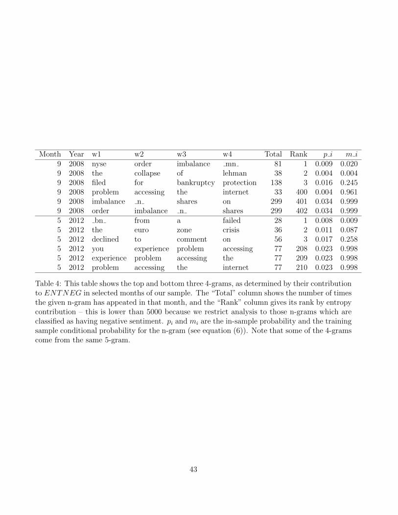
Month Year w1 w2 w3 w4 Total Rank p i m i9 2008 nyse order imbalance mn 81 1 0.009 0.0209 2008 the collapse of lehman 38 2 0.004 0.0049 2008 filed for bankruptcy protection 138 3 0.016 0.2459 2008 problem accessing the internet 33 400 0.004 0.9619 2008 imbalance n shares on 299 401 0.034 0.9999 2008 order imbalance n shares 299 402 0.034 0.9995 2012 bn from a failed 28 1 0.008 0.0095 2012 the euro zone crisis 36 2 0.011 0.0875 2012 declined to comment on 56 3 0.017 0.2585 2012 you experience problem accessing 77 208 0.023 0.9985 2012 experience problem accessing the 77 209 0.023 0.9985 2012 problem accessing the internet 77 210 0.023 0.998

Table 4: This table shows the top and bottom three 4-grams, as determined by their contributionto ENTNEG in selected months of our sample. The “Total” column shows the number of timesthe given n-gram has appeated in that month, and the “Rank” column gives its rank by entropycontribution – this is lower than 5000 because we restrict analysis to those n-grams which areclassified as having negative sentiment. pi and mi are the in-sample probability and the trainingsample conditional probability for the n-gram (see equation (6)). Note that some of the 4-gramscome from the same 5-gram.

43

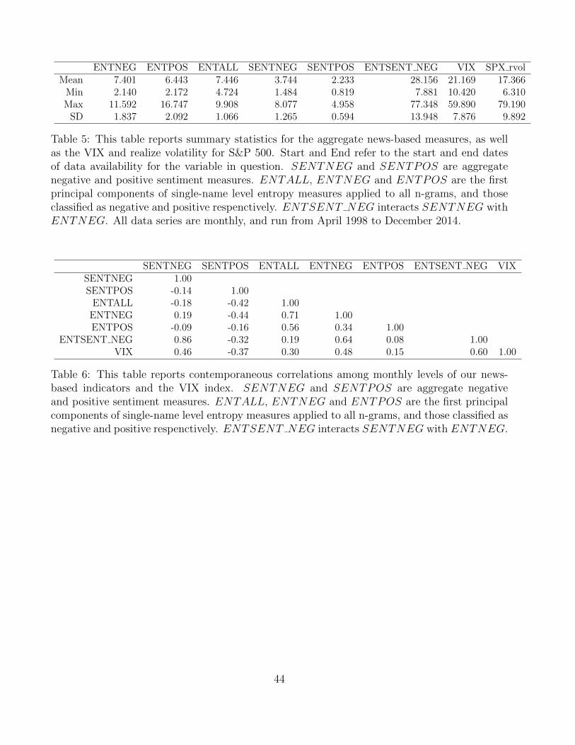
ENTNEG ENTPOS ENTALL SENTNEG SENTPOS ENTSENT NEG VIX SPX rvolMean 7.401 6.443 7.446 3.744 2.233 28.156 21.169 17.366

Min 2.140 2.172 4.724 1.484 0.819 7.881 10.420 6.310Max 11.592 16.747 9.908 8.077 4.958 77.348 59.890 79.190

SD 1.837 2.092 1.066 1.265 0.594 13.948 7.876 9.892

Table 5: This table reports summary statistics for the aggregate news-based measures, as wellas the VIX and realize volatility for S&P 500. Start and End refer to the start and end datesof data availability for the variable in question. SENTNEG and SENTPOS are aggregatenegative and positive sentiment measures. ENTALL, ENTNEG and ENTPOS are the firstprincipal components of single-name level entropy measures applied to all n-grams, and thoseclassified as negative and positive respenctively. ENTSENT NEG interacts SENTNEG withENTNEG. All data series are monthly, and run from April 1998 to December 2014.

SENTNEG SENTPOS ENTALL ENTNEG ENTPOS ENTSENT NEG VIXSENTNEG 1.00SENTPOS -0.14 1.00

ENTALL -0.18 -0.42 1.00ENTNEG 0.19 -0.44 0.71 1.00ENTPOS -0.09 -0.16 0.56 0.34 1.00

ENTSENT NEG 0.86 -0.32 0.19 0.64 0.08 1.00VIX 0.46 -0.37 0.30 0.48 0.15 0.60 1.00

Table 6: This table reports contemporaneous correlations among monthly levels of our news-based indicators and the VIX index. SENTNEG and SENTPOS are aggregate negativeand positive sentiment measures. ENTALL, ENTNEG and ENTPOS are the first principalcomponents of single-name level entropy measures applied to all n-grams, and those classified asnegative and positive respenctively. ENTSENT NEG interacts SENTNEG with ENTNEG.

44

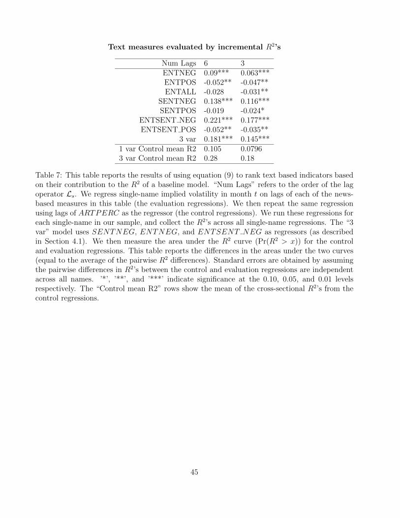
Text measures evaluated by incremental R2’s

Num Lags 6 3ENTNEG 0.09*** 0.063***ENTPOS -0.052** -0.047**ENTALL -0.028 -0.031**

SENTNEG 0.138*** 0.116***SENTPOS -0.019 -0.024*

ENTSENT NEG 0.221*** 0.177***ENTSENT POS -0.052** -0.035**

3 var 0.181*** 0.145***1 var Control mean R2 0.105 0.07963 var Control mean R2 0.28 0.18

Table 7: This table reports the results of using equation (9) to rank text based indicators basedon their contribution to the R2 of a baseline model. “Num Lags” refers to the order of the lagoperator Ls. We regress single-name implied volatility in month t on lags of each of the news-based measures in this table (the evaluation regressions). We then repeat the same regressionusing lags of ARTPERC as the regressor (the control regressions). We run these regressions foreach single-name in our sample, and collect the R2’s across all single-name regressions. The “3var” model uses SENTNEG, ENTNEG, and ENTSENT NEG as regressors (as describedin Section 4.1). We then measure the area under the R2 curve (Pr(R2 > x)) for the controland evaluation regressions. This table reports the differences in the areas under the two curves(equal to the average of the pairwise R2 differences). Standard errors are obtained by assumingthe pairwise differences in R2’s between the control and evaluation regressions are independentacross all names. ’*’, ’**’, and ’***’ indicate significance at the 0.10, 0.05, and 0.01 levelsrespectively. The “Control mean R2” rows show the mean of the cross-sectional R2’s from thecontrol regressions.

45

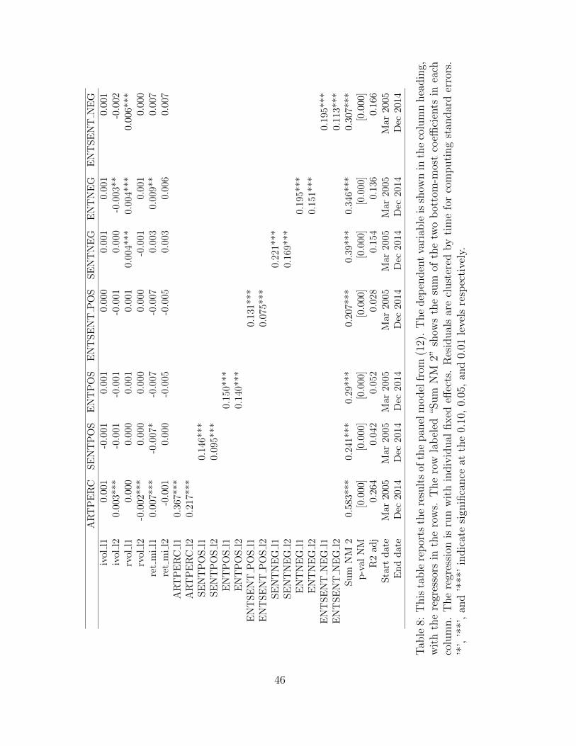
AR

TP

ER

CS

EN

TP

OS

EN

TP

OS

EN

TS

EN

TP

OS

SE

NT

NE

GE

NT

NE

GE

NT

SE

NT

NE

Giv

oll1

0.00

1-0

.001

0.00

10.

000

0.00

10.

001

0.00

1iv

oll2

0.00

3***

-0.0

01-0

.001

-0.0

010.

000

-0.0

03**

-0.0

02rv

oll1

0.00

00.

000

0.00

10.

001

0.00

4***

0.00

4***

0.00

6***

rvol

l2-0

.002

***

0.00

00.

000

0.00

0-0

.001

0.00

10.

000

ret

mi

l10.

007*

**-0

.007

*-0

.007

-0.0

070.

003

0.00

9**

0.00

7re

tm

il2

-0.0

010.

000

-0.0

05-0

.005

0.00

30.

006

0.00

7A

RT

PE

RC

l10.

367*

**A

RT

PE

RC

l20.

217*

**S

EN

TP

OS

l10.

146*

**S

EN

TP

OS

l20.

095*

**E

NT

PO

Sl1

0.15

0***

EN

TP

OS

l20.

140*

**E

NT

SE

NT

PO

Sl1

0.13

1***

EN

TS

EN

TP

OS

l20.

075*

**S

EN

TN

EG

l10.

221*

**S

EN

TN

EG

l20.

169*

**E

NT

NE

Gl1

0.19

5***

EN

TN

EG

l20.

151*

**E

NT

SE

NT

NE

Gl1

0.19

5***

EN

TS

EN

TN

EG

l20.

113*

**S

um

NM

20.

583*

**0.

241*

**0.

29**

*0.

207*

**0.

39**

*0.

346*

**0.

307*

**p

-val

NM

[0.0

00]

[0.0

00]

[0.0

00]

[0.0

00]

[0.0

00]

[0.0

00]

[0.0

00]

R2

adj

0.26

40.

042

0.05

20.

028

0.15

40.

136

0.16

6S

tart

dat

eM

ar20

05M

ar20

05M

ar20

05M

ar20

05M

ar20

05M

ar20

05M

ar20

05E

nd

dat

eD

ec20

14D

ec20

14D

ec20

14D

ec20

14D

ec20

14D

ec20

14D

ec20

14

Tab

le8:

This

table

rep

orts

the

resu

lts

ofth

epan

elm

odel

from

(12)

.T

he

dep

enden

tva

riab

leis

show

nin

the

colu

mn

hea

din

g,w

ith

the

regr

esso

rsin

the

row

s.T

he

row

lab

eled

“Sum

NM

2”sh

ows

the

sum

ofth

etw

ob

otto

m-m

ost

coeffi

cien

tsin

each

colu

mn.

The

regr

essi

onis

run

wit

hin

div

idual

fixed

effec

ts.

Res

idual

sar

ecl

ust

ered

by

tim

efo

rco

mputi

ng

stan

dar

der

rors

.’*

’,’*

*’,

and

’***

’in

dic

ate

sign

ifica

nce

atth

e0.

10,

0.05

,an

d0.

01le

vels

resp

ecti

vely

.

46

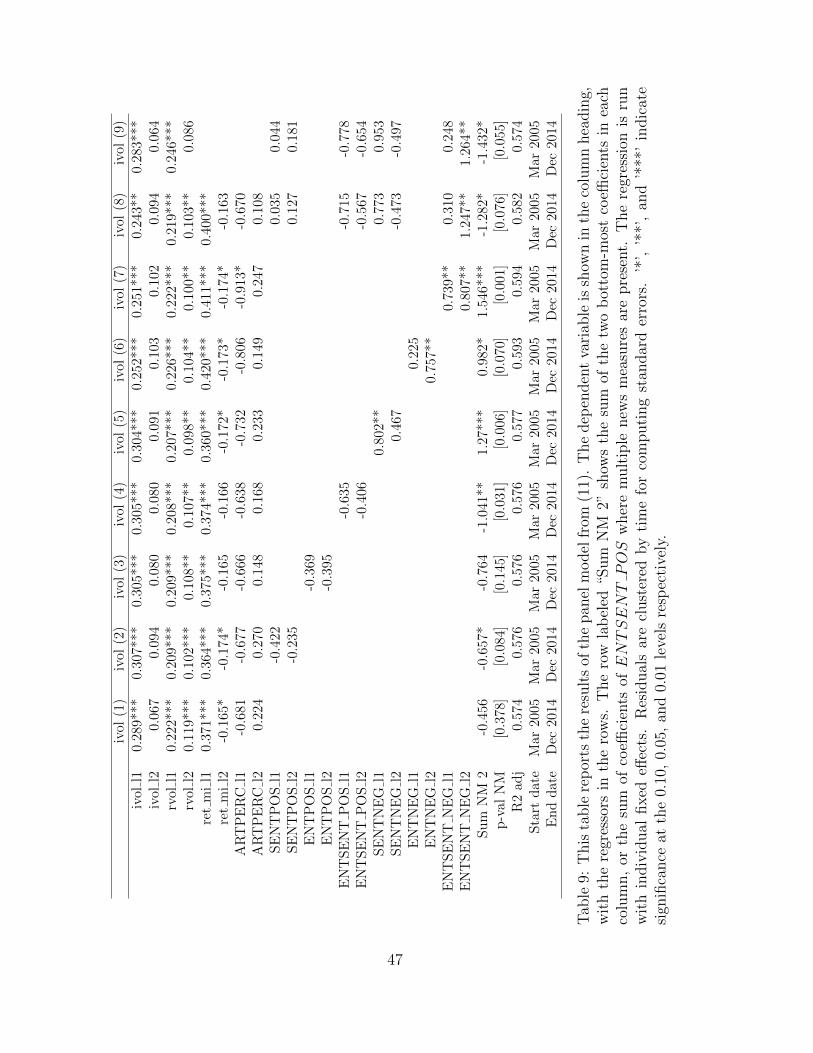
ivol

(1)

ivol

(2)

ivol

(3)

ivol

(4)

ivol

(5)

ivol

(6)

ivol

(7)

ivol

(8)

ivol

(9)

ivol

l10.

289*

**0.

307*

**0.

305*

**0.

305*

**0.

304*

**0.

252*

**0.

251*

**0.

243*

*0.

283*

**iv

oll2

0.06

70.

094

0.08

00.

080

0.09

10.

103

0.10

20.

094

0.06

4rv

oll1

0.22

2***

0.20

9***

0.20

9***

0.20

8***

0.20

7***

0.22

6***

0.22

2***

0.21

9***

0.24

6***

rvol

l20.

119*

**0.

102*

**0.

108*

*0.

107*

*0.

098*

*0.

104*

*0.

100*

*0.

103*

*0.

086

ret

mi

l10.

371*

**0.

364*

**0.

375*

**0.

374*

**0.

360*

**0.

420*

**0.

411*

**0.

400*

**re

tm

il2

-0.1

65*

-0.1

74*

-0.1

65-0

.166

-0.1

72*

-0.1

73*

-0.1

74*

-0.1

63A

RT

PE

RC

l1-0

.681

-0.6

77-0

.666

-0.6

38-0

.732

-0.8

06-0

.913

*-0

.670

AR

TP

ER

Cl2

0.22

40.

270

0.14

80.

168

0.23

30.

149

0.24

70.

108

SE

NT

PO

Sl1

-0.4

220.

035

0.04

4S

EN

TP

OS

l2-0

.235

0.12

70.

181

EN

TP

OS

l1-0

.369

EN

TP

OS

l2-0

.395

EN

TS

EN

TP

OS

l1-0

.635

-0.7

15-0

.778

EN

TS

EN

TP

OS

l2-0

.406

-0.5

67-0

.654

SE

NT

NE

Gl1

0.80

2**

0.77

30.

953

SE

NT

NE

Gl2

0.46

7-0

.473

-0.4

97E

NT

NE

Gl1

0.22

5E

NT

NE

Gl2

0.75

7**

EN

TS

EN

TN

EG

l10.

739*

*0.

310

0.24

8E

NT

SE

NT

NE

Gl2

0.80

7**

1.24

7**

1.26

4**

Su

mN

M2

-0.4

56-0

.657

*-0

.764

-1.0

41**

1.27

***

0.98

2*1.

546*

**-1

.282

*-1

.432

*p

-val

NM

[0.3

78]

[0.0

84]

[0.1

45]

[0.0

31]

[0.0

06]

[0.0

70]

[0.0

01]

[0.0

76]

[0.0

55]

R2

adj

0.57

40.

576

0.57

60.

576

0.57

70.

593

0.59

40.

582

0.57

4S

tart

dat

eM

ar20

05M

ar20

05M

ar20

05M

ar20

05M

ar20

05M

ar20

05M

ar20

05M

ar20

05M

ar20

05E

nd

dat

eD

ec20

14D

ec20

14D

ec20

14D

ec20

14D

ec20

14D

ec20

14D

ec20

14D

ec20

14D

ec20

14

Tab

le9:

This

table

rep

orts

the

resu

lts

ofth

epan

elm

odel

from

(11)

.T

he

dep

enden

tva

riab

leis

show

nin

the

colu

mn

hea

din

g,w

ith

the

regr

esso

rsin

the

row

s.T

he

row

lab

eled

“Sum

NM

2”sh

ows

the

sum

ofth

etw

ob

otto

m-m

ost

coeffi

cien

tsin

each

colu

mn,

orth

esu

mof

coeffi

cien

tsofENTSENTPOS

wher

em

ult

iple

new

sm

easu

res

are

pre

sent.

The

regr

essi

onis

run

wit

hin

div

idual

fixed

effec

ts.

Res

idual

sar

ecl

ust

ered

by

tim

efo

rco

mputi

ng

stan

dar

der

rors

.’*

’,’*

*’,

and

’***

’in

dic

ate

sign

ifica

nce

atth

e0.

10,

0.05

,an

d0.

01le

vels

resp

ecti

vely

.

47

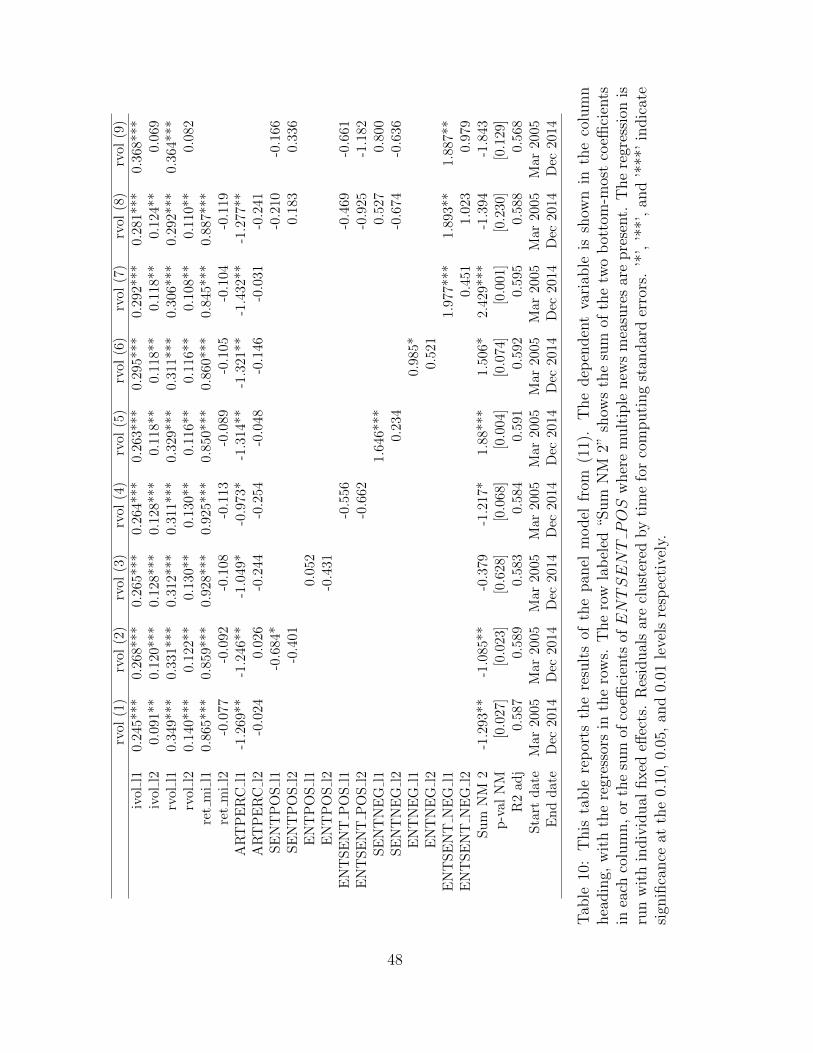
rvol

(1)

rvol

(2)

rvol

(3)

rvol

(4)

rvol

(5)

rvol

(6)

rvol

(7)

rvol

(8)

rvol

(9)

ivol

l10.

245*

**0.

268*

**0.

265*

**0.

264*

**0.

263*

**0.

295*

**0.

292*

**0.

281*

**0.

368*

**iv

oll2

0.09

1**

0.12

0***

0.12

8***

0.12

8***

0.11

8**

0.11

8**

0.11

8**

0.12

4**

0.06

9rv

oll1

0.34

9***

0.33

1***

0.31

2***

0.31

1***

0.32

9***

0.31

1***

0.30

6***

0.29

2***

0.36

4***

rvol

l20.

140*

**0.

122*

*0.

130*

*0.

130*

*0.

116*

*0.

116*

*0.

108*

*0.

110*

*0.

082

ret

mi

l10.

865*

**0.

859*

**0.

928*

**0.

925*

**0.

850*

**0.

860*

**0.

845*

**0.

887*

**re

tm

il2

-0.0

77-0

.092

-0.1

08-0

.113

-0.0

89-0

.105

-0.1

04-0

.119

AR

TP

ER

Cl1

-1.2

69**

-1.2

46**

-1.0

49*

-0.9

73*

-1.3

14**

-1.3

21**

-1.4

32**

-1.2

77**

AR

TP

ER

Cl2

-0.0

240.

026

-0.2

44-0

.254

-0.0

48-0

.146

-0.0

31-0

.241

SE

NT

PO

Sl1

-0.6

84*

-0.2

10-0

.166

SE

NT

PO

Sl2

-0.4

010.

183

0.33

6E

NT

PO

Sl1

0.05

2E

NT

PO

Sl2

-0.4

31E

NT

SE

NT

PO

Sl1

-0.5

56-0

.469

-0.6

61E

NT

SE

NT

PO

Sl2

-0.6

62-0

.925

-1.1

82S

EN

TN

EG

l11.

646*

**0.

527

0.80

0S

EN

TN

EG

l20.

234

-0.6

74-0

.636

EN

TN

EG

l10.

985*

EN

TN

EG

l20.

521

EN

TS

EN

TN

EG

l11.

977*

**1.

893*

*1.

887*

*E

NT

SE

NT

NE

Gl2

0.45

11.

023

0.97

9S

um

NM

2-1

.293

**-1

.085

**-0

.379

-1.2

17*

1.88

***

1.50

6*2.

429*

**-1

.394

-1.8

43p

-val

NM

[0.0

27]

[0.0

23]

[0.6

28]

[0.0

68]

[0.0

04]

[0.0

74]

[0.0

01]

[0.2

30]

[0.1

29]

R2

adj

0.58

70.

589

0.58

30.

584

0.59

10.

592

0.59

50.

588

0.56

8S

tart

dat

eM

ar20

05M

ar20

05M

ar20

05M

ar20

05M

ar20

05M

ar20

05M

ar20

05M

ar20

05M

ar20

05E

nd

dat

eD

ec20

14D

ec20

14D

ec20

14D

ec20

14D

ec20

14D

ec20

14D

ec20

14D

ec20

14D

ec20

14

Tab

le10

:T

his

table

rep

orts

the

resu

lts

ofth

epan

elm

odel

from

(11)

.T

he

dep

enden

tva

riab

leis

show

nin

the

colu

mn

hea

din

g,w

ith

the

regr

esso

rsin

the

row

s.T

he

row

lab

eled

“Sum

NM

2”sh

ows

the

sum

ofth

etw

ob

otto

m-m

ost

coeffi

cien

tsin

each

colu

mn,

orth

esu

mof

coeffi

cien

tsofENTSENTPOS

wher

em

ult

iple

new

sm

easu

res

are

pre

sent.

The

regr

essi

onis

run

wit

hin

div

idual

fixed

effec

ts.

Res

idual

sar

ecl

ust

ered

by

tim

efo

rco

mputi

ng

stan

dar

der

rors

.’*

’,’*

*’,

and

’***

’in

dic

ate

sign

ifica

nce

atth

e0.

10,

0.05

,an

d0.

01le

vels

resp

ecti

vely

.

48

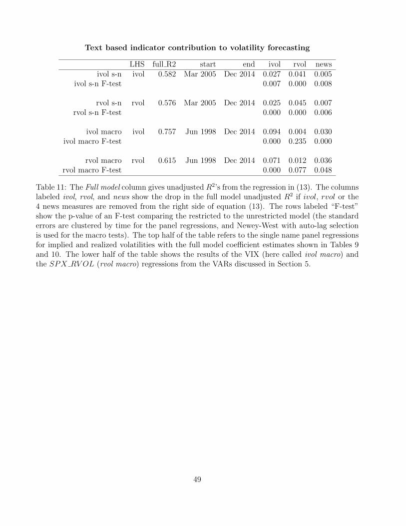
Text based indicator contribution to volatility forecasting

LHS full R2 start end ivol rvol newsivol s-n ivol 0.582 Mar 2005 Dec 2014 0.027 0.041 0.005

ivol s-n F-test 0.007 0.000 0.008

rvol s-n rvol 0.576 Mar 2005 Dec 2014 0.025 0.045 0.007rvol s-n F-test 0.000 0.000 0.006

ivol macro ivol 0.757 Jun 1998 Dec 2014 0.094 0.004 0.030ivol macro F-test 0.000 0.235 0.000

rvol macro rvol 0.615 Jun 1998 Dec 2014 0.071 0.012 0.036rvol macro F-test 0.000 0.077 0.048

Table 11: The Full model column gives unadjusted R2’s from the regression in (13). The columnslabeled ivol, rvol, and news show the drop in the full model unadjusted R2 if ivol, rvol or the4 news measures are removed from the right side of equation (13). The rows labeled “F-test”show the p-value of an F-test comparing the restricted to the unrestricted model (the standarderrors are clustered by time for the panel regressions, and Newey-West with auto-lag selectionis used for the macro tests). The top half of the table refers to the single name panel regressionsfor implied and realized volatilities with the full model coefficient estimates shown in Tables 9and 10. The lower half of the table shows the results of the VIX (here called ivol macro) andthe SPX RV OL (rvol macro) regressions from the VARs discussed in Section 5.

49

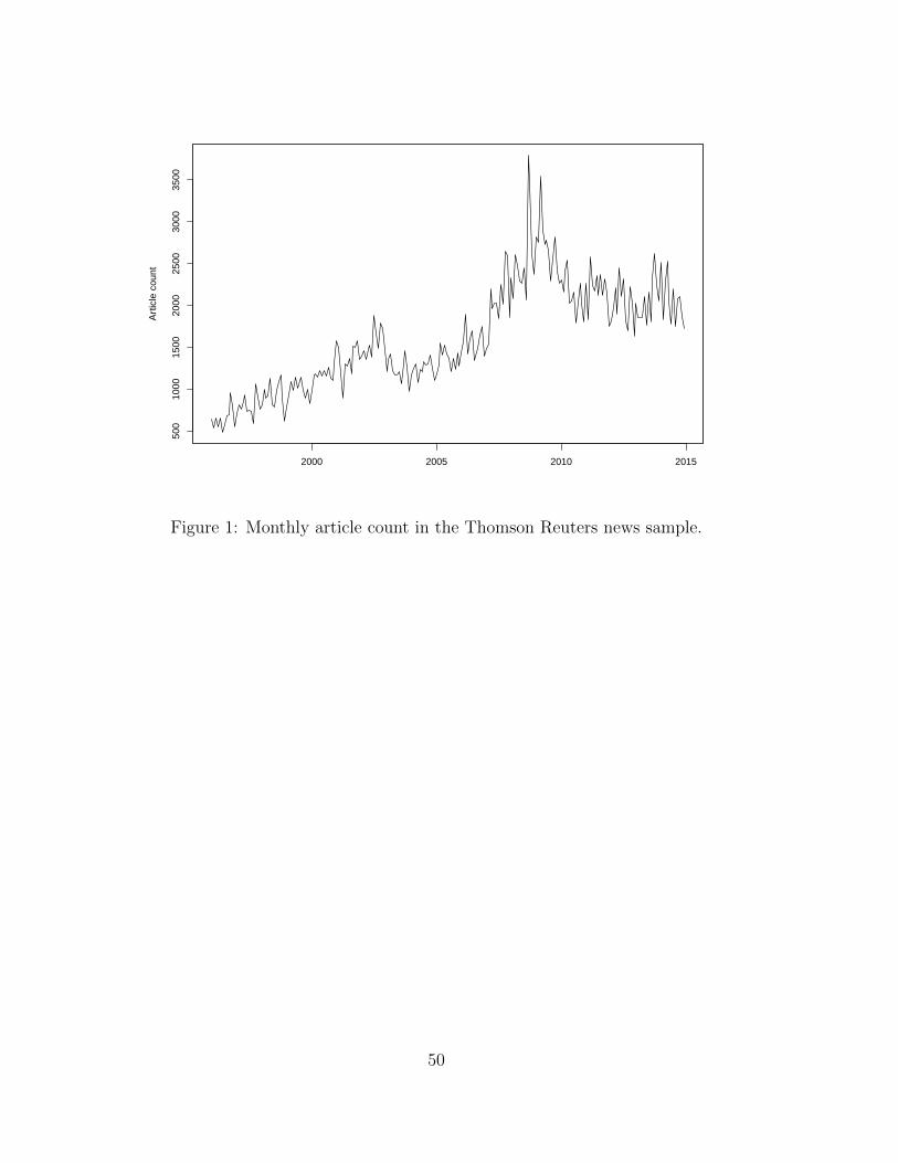
2000 2005 2010 2015

500

1000

1500

2000

2500

3000

3500

Art

icle

cou

nt

Figure 1: Monthly article count in the Thomson Reuters news sample.

50

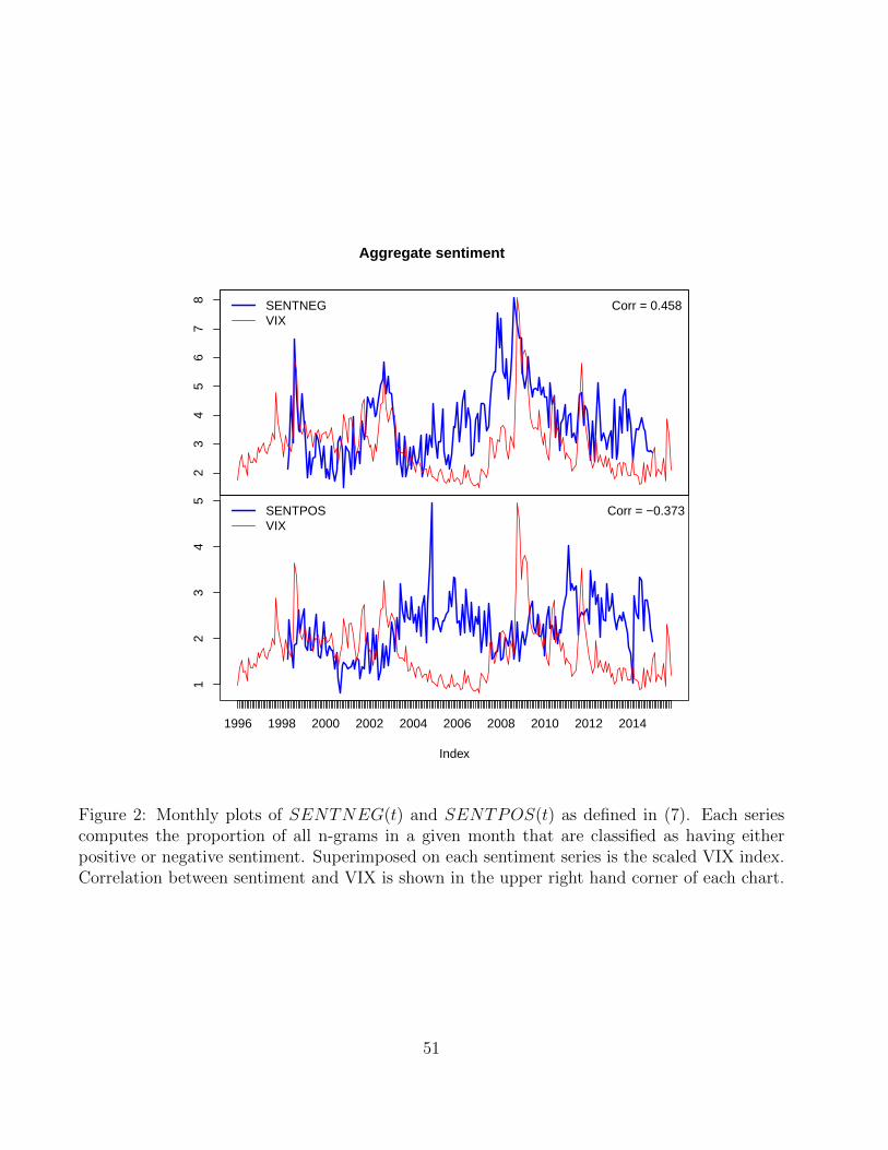
23

45

67

8 SENTNEGVIX

Corr = 0.458

1996 1998 2000 2002 2004 2006 2008 2010 2012 2014

Index

12

34

5

SENTPOSVIX

Corr = −0.373

Aggregate sentiment

Figure 2: Monthly plots of SENTNEG(t) and SENTPOS(t) as defined in (7). Each seriescomputes the proportion of all n-grams in a given month that are classified as having eitherpositive or negative sentiment. Superimposed on each sentiment series is the scaled VIX index.Correlation between sentiment and VIX is shown in the upper right hand corner of each chart.

51

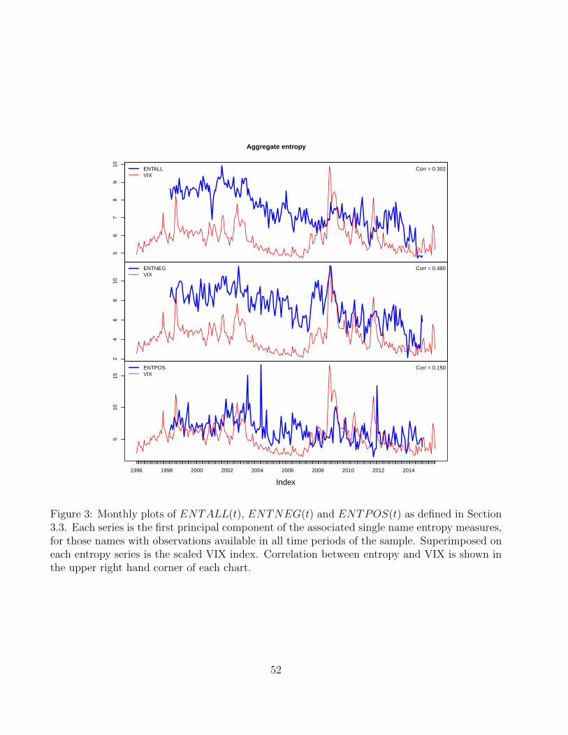
56

78

910

ENTALLVIX

Corr = 0.302

24

68

10

ENTNEGVIX

Corr = 0.480

1996 1998 2000 2002 2004 2006 2008 2010 2012 2014

Index

510

15

ENTPOSVIX

Corr = 0.150

Aggregate entropy

Figure 3: Monthly plots of ENTALL(t), ENTNEG(t) and ENTPOS(t) as defined in Section3.3. Each series is the first principal component of the associated single name entropy measures,for those names with observations available in all time periods of the sample. Superimposed oneach entropy series is the scaled VIX index. Correlation between entropy and VIX is shown inthe upper right hand corner of each chart.

52

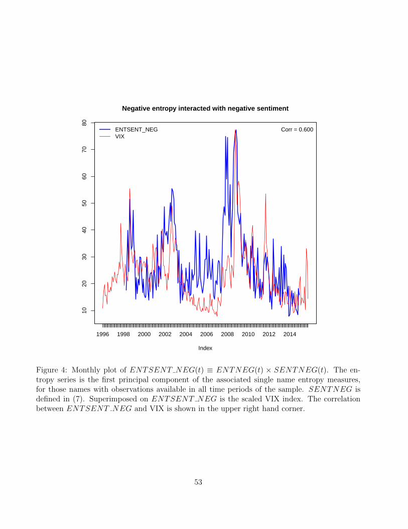
1996 1998 2000 2002 2004 2006 2008 2010 2012 2014

1020

3040

5060

7080

Index

ENTSENT_NEGVIX

Corr = 0.600

Negative entropy interacted with negative sentiment

Figure 4: Monthly plot of ENTSENT NEG(t) ≡ ENTNEG(t) × SENTNEG(t). The en-tropy series is the first principal component of the associated single name entropy measures,for those names with observations available in all time periods of the sample. SENTNEG isdefined in (7). Superimposed on ENTSENT NEG is the scaled VIX index. The correlationbetween ENTSENT NEG and VIX is shown in the upper right hand corner.

53

1 2 3 4 5 6

−2

−1

01

2

Mean and 2xSE bands for cross−section of coefficients

Lag

AR

TIC

LE_P

ER

CTO

T

●●

●●

●

●

●●

●●

●●●

●●●●●●●

●●●●●●●●●●●●●●●●●●●●●●●●●●●●●

1.0 0.8 0.6 0.4 0.2 0.00.

00.

20.

40.

60.

81.

0

1−CDF for R2

r2

Pr(

R2

> x

)

Market data regressed onlagged forecasting variables.Names in cross−section = 41Minimum observations = 60

Reg summary for future implied vol on article count lags=6 ivol=false fwd step=0

Figure 5: The results of the regression in (9) with NEWSj set to the percentage of articlesin month t that mention company j. The ARTPERC variables are normalized to have unitstandard deviation. Shown are the cross-sectional mean of each coefficient with a two standarderror band, and a plot of 1 minus the cumulative distribution function of the unadjusted R2’sfrom the single name regressions, i.e. f(x) = Pr(R2 > x), with ARTPERC as the right handside variable. Note the x-axis starts at 1 and decreases to 0. Data are monthly.

54

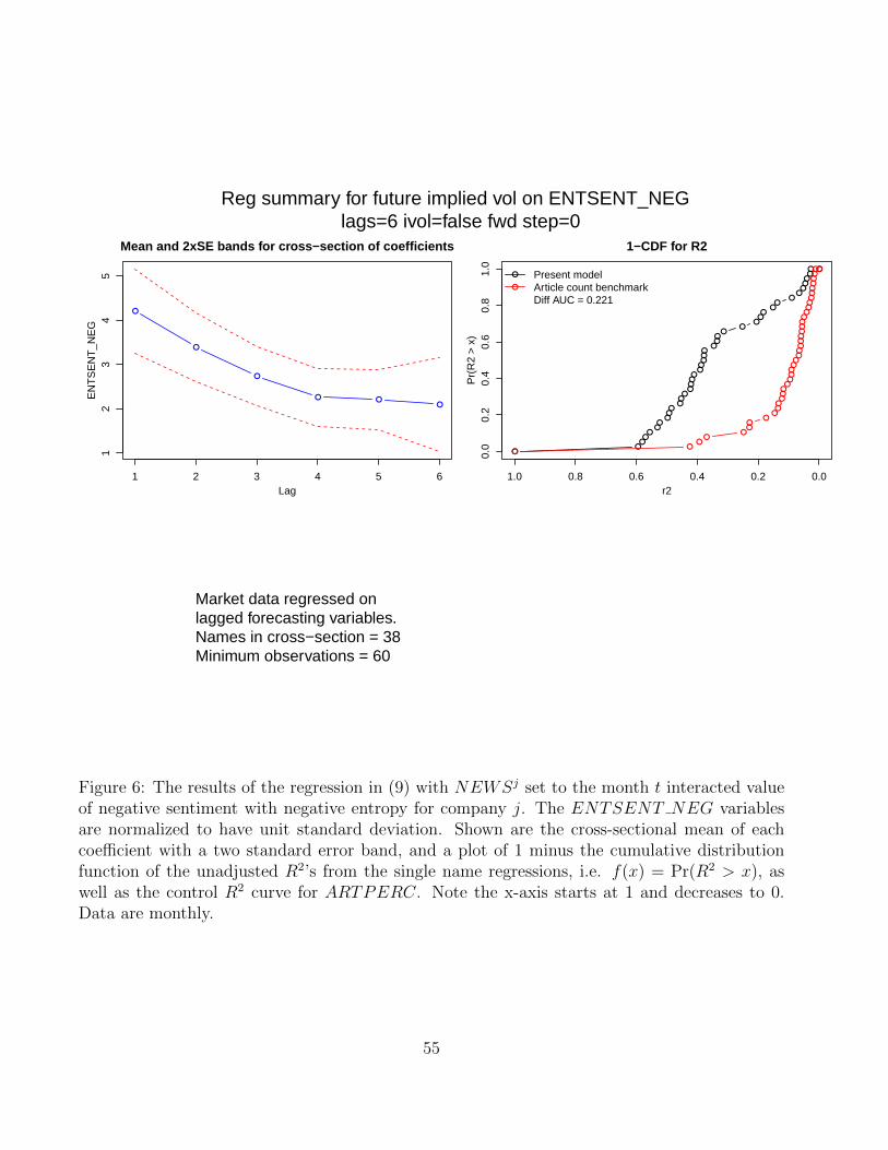
1 2 3 4 5 6

12

34

5

Mean and 2xSE bands for cross−section of coefficients

Lag

EN

TS

EN

T_N

EG

●

●

●

● ●●

●●

●●

●●●

●●●

●●●

●●●●

●●●●●

●●●

●●

●●●

●●

●●

●●●●● ●

1.0 0.8 0.6 0.4 0.2 0.00.

00.

20.

40.

60.

81.

0

1−CDF for R2

r2

Pr(

R2

> x

)

●●

●●

●●●

●●●●●●●

●●●●●●●●●●●●●●●●●●●●●●●●●●

●

●

Present modelArticle count benchmarkDiff AUC = 0.221

Market data regressed onlagged forecasting variables.Names in cross−section = 38Minimum observations = 60

Reg summary for future implied vol on ENTSENT_NEG lags=6 ivol=false fwd step=0

Figure 6: The results of the regression in (9) with NEWSj set to the month t interacted valueof negative sentiment with negative entropy for company j. The ENTSENT NEG variablesare normalized to have unit standard deviation. Shown are the cross-sectional mean of eachcoefficient with a two standard error band, and a plot of 1 minus the cumulative distributionfunction of the unadjusted R2’s from the single name regressions, i.e. f(x) = Pr(R2 > x), aswell as the control R2 curve for ARTPERC. Note the x-axis starts at 1 and decreases to 0.Data are monthly.

55

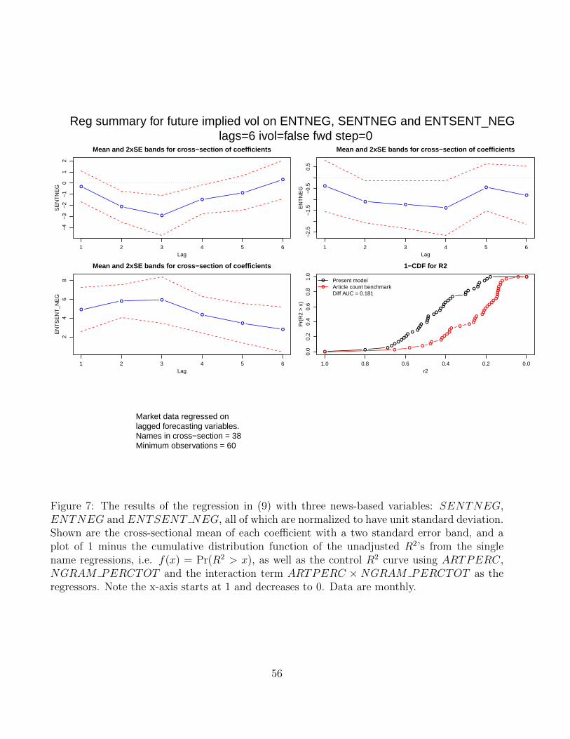
1 2 3 4 5 6

−4

−3

−2

−1

01

2

Mean and 2xSE bands for cross−section of coefficients

Lag

SE

NT

NE

G ●

●

●

●

●

●

1 2 3 4 5 6

−2.

5−

1.5

−0.

50.

5

Mean and 2xSE bands for cross−section of coefficients

Lag

EN

TN

EG

●

●●

●

●

●

1 2 3 4 5 6

24

68

Mean and 2xSE bands for cross−section of coefficients

Lag

EN

TS

EN

T_N

EG

●

● ●

●

●

●

●●

●●

●●

●●

●●

●●●●●

●●●●

●●

●●

●●●

●●

●●●

●●

●●●

●●

● ●

1.0 0.8 0.6 0.4 0.2 0.0

0.0

0.2

0.4

0.6

0.8

1.0

1−CDF for R2

r2

Pr(

R2

> x

)

●●

●●

●●

●●

●●

●●●

●●

●●●●

●●●●●

●●●

●●●●●●●●●●

●● ●

●

●

Present modelArticle count benchmarkDiff AUC = 0.181

Market data regressed onlagged forecasting variables.Names in cross−section = 38Minimum observations = 60

Reg summary for future implied vol on ENTNEG, SENTNEG and ENTSENT_NEG lags=6 ivol=false fwd step=0

Figure 7: The results of the regression in (9) with three news-based variables: SENTNEG,ENTNEG and ENTSENT NEG, all of which are normalized to have unit standard deviation.Shown are the cross-sectional mean of each coefficient with a two standard error band, and aplot of 1 minus the cumulative distribution function of the unadjusted R2’s from the singlename regressions, i.e. f(x) = Pr(R2 > x), as well as the control R2 curve using ARTPERC,NGRAM PERCTOT and the interaction term ARTPERC × NGRAM PERCTOT as theregressors. Note the x-axis starts at 1 and decreases to 0. Data are monthly.

56

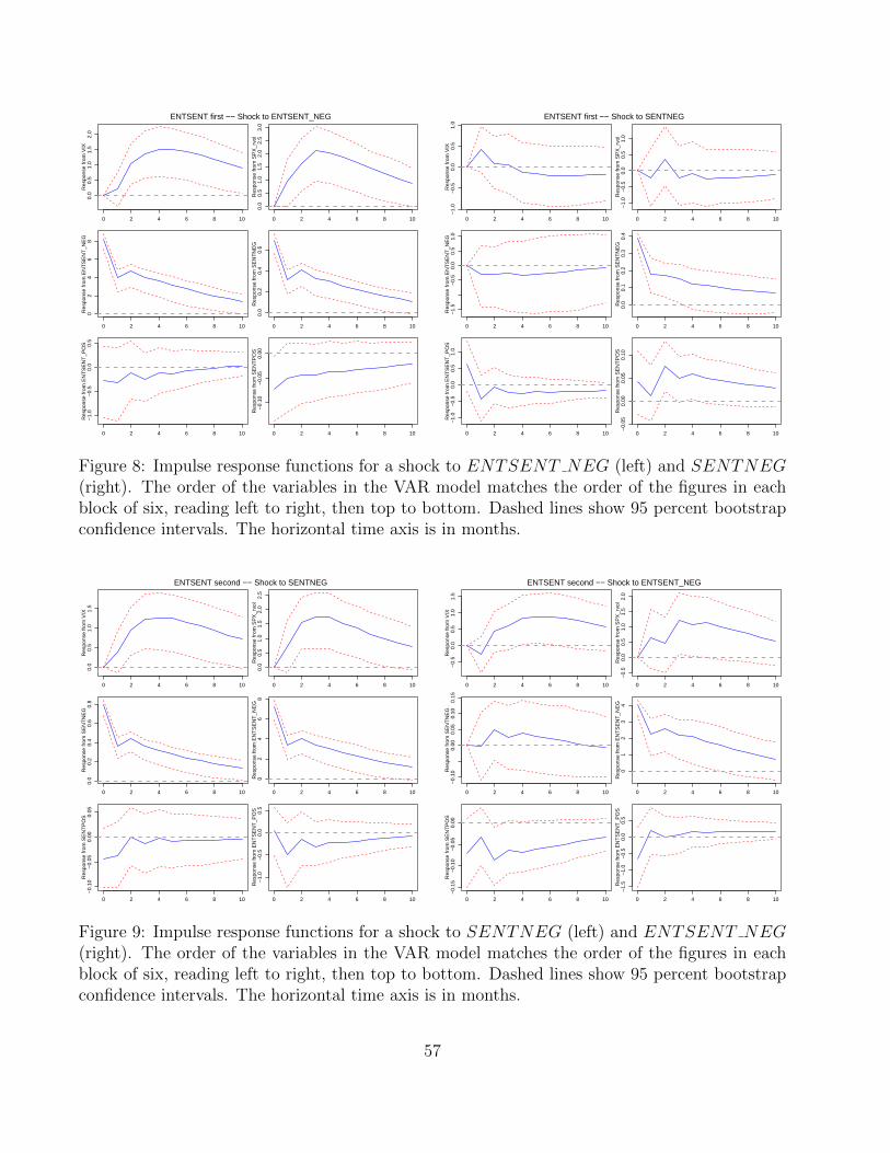
0 2 4 6 8 10

0.0

0.5

1.0

1.5

2.0

Res

pons

e fr

om V

IX

0 2 4 6 8 10

0.0

0.5

1.0

1.5

2.0

2.5

3.0

Res

pons

e fr

om S

PX

_rvo

l

0 2 4 6 8 10

02

46

8R

espo

nse

from

EN

TS

EN

T_N

EG

0 2 4 6 8 10

0.0

0.2

0.4

0.6

Res

pons

e fr

om S

EN

TN

EG

0 2 4 6 8 10

−1.

0−

0.5

0.0

0.5

Res

pons

e fr

om E

NT

SE

NT

_PO

S

0 2 4 6 8 10

−0.

10−

0.05

0.00

Res

pons

e fr

om S

EN

TP

OS

ENTSENT first −− Shock to ENTSENT_NEG

0 2 4 6 8 10

−1.

0−

0.5

0.0

0.5

1.0

Res

pons

e fr

om V

IX

0 2 4 6 8 10

−1.

0−

0.5

0.0

0.5

1.0

Res

pons

e fr

om S

PX

_rvo

l

0 2 4 6 8 10

−1.

5−

0.5

0.0

0.5

1.0

Res

pons

e fr

om E

NT

SE

NT

_NE

G

0 2 4 6 8 10

0.0

0.1

0.2

0.3

0.4

Res

pons

e fr

om S

EN

TN

EG

0 2 4 6 8 10

−1.

0−

0.5

0.0

0.5

1.0

Res

pons

e fr

om E

NT

SE

NT

_PO

S

0 2 4 6 8 10

−0.

050.

000.

050.

10R

espo

nse

from

SE

NT

PO

S

ENTSENT first −− Shock to SENTNEG

Figure 8: Impulse response functions for a shock to ENTSENT NEG (left) and SENTNEG(right). The order of the variables in the VAR model matches the order of the figures in eachblock of six, reading left to right, then top to bottom. Dashed lines show 95 percent bootstrapconfidence intervals. The horizontal time axis is in months.

0 2 4 6 8 10

0.0

0.5

1.0

1.5

Res

pons

e fr

om V

IX

0 2 4 6 8 10

0.0

0.5

1.0

1.5

2.0

2.5

Res

pons

e fr

om S

PX

_rvo

l

0 2 4 6 8 10

0.0

0.2

0.4

0.6

0.8

Res

pons

e fr

om S

EN

TN

EG

0 2 4 6 8 10

02

46

8R

espo

nse

from

EN

TS

EN

T_N

EG

0 2 4 6 8 10

−0.

10−

0.05

0.00

0.05

Res

pons

e fr

om S

EN

TP

OS

0 2 4 6 8 10

−1.

0−

0.5

0.0

0.5

Res

pons

e fr

om E

NT

SE

NT

_PO

S

ENTSENT second −− Shock to SENTNEG

0 2 4 6 8 10

−0.

50.

00.

51.

01.

5R

espo

nse

from

VIX

0 2 4 6 8 10

−0.

50.

00.

51.

01.

52.

0R

espo

nse

from

SP

X_r

vol

0 2 4 6 8 10

−0.

100.

000.

050.

100.

15R

espo

nse

from

SE

NT

NE

G

0 2 4 6 8 10

01

23

4R

espo

nse

from

EN

TS

EN

T_N

EG

0 2 4 6 8 10

−0.

15−

0.10

−0.

050.

00R

espo

nse

from

SE

NT

PO

S

0 2 4 6 8 10

−1.

5−

1.0

−0.

50.

00.

5R

espo

nse

from

EN

TS

EN

T_P

OS

ENTSENT second −− Shock to ENTSENT_NEG

Figure 9: Impulse response functions for a shock to SENTNEG (left) and ENTSENT NEG(right). The order of the variables in the VAR model matches the order of the figures in eachblock of six, reading left to right, then top to bottom. Dashed lines show 95 percent bootstrapconfidence intervals. The horizontal time axis is in months.

57

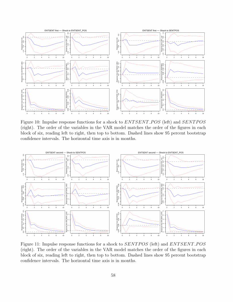
0 2 4 6 8 10

−1.

5−

1.0

−0.

50.

0R

espo

nse

from

VIX

0 2 4 6 8 10

−2.

0−

1.0

0.0

0.5

Res

pons

e fr

om S

PX

_rvo

l

0 2 4 6 8 10

−2

−1

01

Res

pons

e fr

om E

NT

SE

NT

_NE

G

0 2 4 6 8 10

−0.

2−

0.1

0.0

0.1

Res

pons

e fr

om S

EN

TN

EG

0 2 4 6 8 10

01

23

45

6R

espo

nse

from

EN

TS

EN

T_P

OS

0 2 4 6 8 10

0.00

0.10

0.20

0.30

Res

pons

e fr

om S

EN

TP

OS

ENTSENT first −− Shock to ENTSENT_POS

0 2 4 6 8 10

−1.

0−

0.5

0.0

0.5

Res

pons

e fr

om V

IX

0 2 4 6 8 10

−1.

5−

1.0

−0.

50.

00.

51.

0R

espo

nse

from

SP

X_r

vol

0 2 4 6 8 10

−1.

00.

00.

51.

01.

5R

espo

nse

from

EN

TS

EN

T_N

EG

0 2 4 6 8 10

−0.

050.

050.

100.

15R

espo

nse

from

SE

NT

NE

G

0 2 4 6 8 10

−0.

50.

00.

5R

espo

nse

from

EN

TS

EN

T_P

OS

0 2 4 6 8 10

0.0

0.1

0.2

0.3

0.4

Res

pons

e fr

om S

EN

TP

OS

ENTSENT first −− Shock to SENTPOS

Figure 10: Impulse response functions for a shock to ENTSENT POS (left) and SENTPOS(right). The order of the variables in the VAR model matches the order of the figures in eachblock of six, reading left to right, then top to bottom. Dashed lines show 95 percent bootstrapconfidence intervals. The horizontal time axis is in months.

0 2 4 6 8 10

−1.

5−

1.0

−0.

50.

00.

5R

espo

nse

from

VIX

0 2 4 6 8 10

−2.

0−

1.0

0.0

0.5

Res

pons

e fr

om S

PX

_rvo

l

0 2 4 6 8 10

−0.

15−

0.05

0.05

0.15

Res

pons

e fr

om S

EN

TN

EG

0 2 4 6 8 10

−2

−1

01

Res

pons

e fr

om E

NT

SE

NT

_NE

G

0 2 4 6 8 10

0.0

0.1

0.2

0.3

0.4

0.5

Res

pons

e fr

om S

EN

TP

OS

0 2 4 6 8 10

01

23

Res

pons

e fr

om E

NT

SE

NT

_PO

S

ENTSENT second −− Shock to SENTPOS

0 2 4 6 8 10

−1.

0−

0.5

0.0

Res

pons

e fr

om V

IX

0 2 4 6 8 10

−1.

5−

1.0

−0.

50.

00.

5R

espo

nse

from

SP

X_r

vol

0 2 4 6 8 10

−0.

25−

0.15

−0.

050.

05R

espo

nse

from

SE

NT

NE

G

0 2 4 6 8 10

−2.

0−

1.0

0.0

0.5

Res

pons

e fr

om E

NT

SE

NT

_NE

G

0 2 4 6 8 10

−0.

050.

000.

050.

10R

espo

nse

from

SE

NT

PO

S

0 2 4 6 8 10

01

23

45

Res

pons

e fr

om E

NT

SE

NT

_PO

S

ENTSENT second −− Shock to ENTSENT_POS

Figure 11: Impulse response functions for a shock to SENTPOS (left) and ENTSENT POS(right). The order of the variables in the VAR model matches the order of the figures in eachblock of six, reading left to right, then top to bottom. Dashed lines show 95 percent bootstrapconfidence intervals. The horizontal time axis is in months.

58

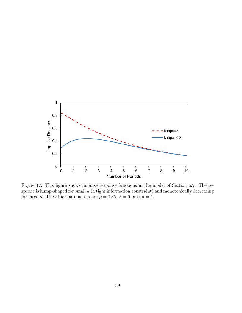
0

0.2

0.4

0.6

0.8

1

0 1 2 3 4 5 6 7 8 9 10

Impu

lse

Res

pons

e

Number of Periods

kappa=3

kappa=0.3

Figure 12: This figure shows impulse response functions in the model of Section 6.2. The re-sponse is hump-shaped for small κ (a tight information constraint) and monotonically decreasingfor large κ. The other parameters are ρ = 0.85, λ = 0, and a = 1.

59