Does Trade Cause Divergence? Dynamic Panel Data Evidence

by

Gabriel J. Felbermayr

Working Paper 0407 June 2004

DDEEPPAARRTTMMEENNTT OOFF EECCOONNOOMMIICCSSJJOOHHAANNNNEESS KKEEPPLLEERR UUNNIIVVEERRSSIITTYY OOFF

LLIINNZZ

Johannes Kepler University of LinzDepartment of Economics

Altenberger Strasse 69A-4040 Linz - Auhof, Austria

www.econ.jku.at

gabriel.felbermayr@jku.atphone +43 (0)70 2468-8265

Does Trade Cause Divergence?

Dynamic Panel Data Evidence.

Gabriel J. Felbermayr¤

June, 2004

Abstract

This paper argues that the empirical trade–growth relationship should be

modelled using a dynamic panel data approach and that it is best estimated with

Blundell and Bond’s (1999) system-GMM estimator. This procedure remedies

some econometric problems such as regressor endogeneity, measurement error

and weak instruments, and allows to control for time-invariant country-speci…c

e¤ects such as institutions or geography. The …ndings are largely plausible and

satisfy intuition better than previous results. They con…rm the existence of a

strong causal e¤ect of trade on growth but fail to …nd evidence for trade as an

independent factor of divergence. Hence, one cannot blame trade as such for the

disappointing performance of initially poor countries.

Keywords: growth empirics, trade, convergence, generalized methods of mo-

ments.

JEL - codes: .F43, O40

¤Johannes Kepler University, Linz, Austria and European University Institute, Florence, Italy. The

author thanks David Roodman for sharing his program codes. Thanks is due to Omar Licandro and

Wilhelm Kohler for numerous discussions and comments.

1 Introduction

This paper has two objectives. First, it argues that the empirical trade-growth re-

lationship should be written as a dynamic panel data model and estimated using the

system-GMM procedure proposed by Blundell and Bond (1998). Second, it applies that

methodology to test a hypothesis frequently found in the earlier endogenous growth

models or in the current popular debate on the e¤ects of globalization, namely, that

international trade is less bene…cial for initially poor countries than it is for more

advanced ones. Is the disappointing growth performance of initially poor countries

causally related to trade liberalization or is it due to other determinants such as insti-

tutional ‡aws or bad governance?

Most economists agree that openness to trade delivers substantial economic ben-

e…ts: according to the classical gains from trade theorem, in an undistorted static

environment, international trade increases the income of a country and helps the rep-

resentative consumer to attain a higher level of utility. While it is possible that the

gains from trade are unevenly distributed between trading partners, there is nothing

in the theory that attributes a decisive role to the initial level of per capita income.

The classical theory is essentially static and requires some rather strong assumptions

such as perfectly competitive markets and the absence of increasing returns to scale.1

A large number of dynamic theoretical papers studies the role of trade openness

in multi-country models of endogenous growth. The older literature emphasizes the

possibility that static comparative advantage may lock poor countries into special-

ization patterns that are not conducive to future productivity growth (Lucas, 1988;

Stokey, 1991; Young, 1991). Depending on the initial value of some state variable (per

capita capital stock, per capita income or the stock of human capital), countries are

sorted into low- and high-productivity-growth groups, while under autarky, all coun-

tries would grow at the same rate. These papers are rather pessimistic because trade1Feenstra (2004) provides an up-to-date review on the theory and empirics of international trade.

2

causes divergence not because of some policy failure or institutional ‡aws, but because

initial conditions place unlucky countries onto the low-growth path. Trade leads to

specialization, which then necessarily implies divergence.

More recently, theorists have provided more detailed arguments why trade may

lead countries to specialize on low productivity growth sectors and/or why trade may

induce a bias in the speed of technical change against some countries (see Gancia,

2003, and the references therein). These papers study the e¤ect of trade liberalization

when countries are a¤ected by other distortions in the form of institutional ‡aws, such

as poor enforcement of property rights. The theory of the second best implies that

in this case trade liberalization can either aggravate or mitigate the adverse e¤ects of

the remaining distortions, so that it may cause some countries to grow more slowly

than others. This stream of research is more optimistic, because it links detrimental

e¤ects of trade to the existence of some distortions which can – in principle – be

removed by institutional reforms.2 Since initially poor countries tend to be those with

poor institutions, the empirical question arises: how can the causal e¤ects of initial

conditions and institutional quality be appropriately separated? The present paper

looks at the interaction between initial income and trade openness and concludes that

trade has not been an engine for divergence in the last-half decade.

In order to estimate the e¤ect of trade on income, empirical researchers typically

run cross-country regressions which are meant to explain income by some measure of

trade openness. This empirical strategy is required, because the direct growth pro-

moting e¤ects of trade – essentially through spillovers are hard to observe empirically.2Of course, in endogenous growth models trade is not necessarily an engine of divergence. The

Schumpeterian research tradition typically concludes that trade leads to convergence. In contrastto Lucas (1988) type models, where there are no international technology spillovers, Grossman andHelpman (1991) and the subsequent R&D based endogenous growth literature, allow for some kind oftechnology di¤usion: either through the public good character of knowledge (chapter 9), or throughthe possibility of poor countries to imitate leaders (chapter 11). In all of these models, trade leadsto income convergence. There are also di¤erent approaches such as Acemoglu and Ventura (2002) orFelbermayr (2004) where trade does not play any role in divergence or convergence.

3

However, in order to identify the causal e¤ect of trade, the researcher has to make

sure that the measure of trade used is orthogonal to the dependent variable. The …rst

paper that uses a convincing instrument to achieve this aim is the one by Frankel and

Romer (1999), who apply a gravity approach to bilateral trade data and construct

trade shares that are by construction orthogonal to income but still strongly correlated

to the actual trade shares. Acemoglu et al. (2001) instrument the quality of institu-

tions with the colonial past of a country. Since then, many other empirical papers have

studied the interaction between per capita income, trade integration and institutions.

However, the vast majority of these models stick with static cross-section regressions,

which assume that all countries are on their respective balanced growth path.3 This as-

sumption is likely to be violated, at the least because the international trading system

has undergone major changes in the last few decades and the speed of convergence,

typically estimated in the empirical literature, is rather small. I reconsider Frankel

and Romer’s (1999) model (henceforth F&R), and, using their instrument for trade,

…nd that it actually performs better in a standard Barro-type cross sectional growth

regression, where conditional convergence is allowed for by including initial income in

the list of covariates.

The present paper uses a rather novel approach to modelling dynamic panel data,

namely, the system-GMM estimator developed by Blundell and Bond (2000). In this

setting, country-speci…c …xed e¤ects such as geographical or time-invariant institutional

characteristics are controlled for by …rst-di¤erencing. Endogenous regressors, in levels

as well as in …rst-di¤erences, are instrumented by their lagged levels. This approach

allows (i) to cast the trade-growth relationship as a dynamic model, (ii) to appropriately3Static regressions focus on the cross-section and relate the level of current per capita income to

trade openness and other regressors. These income regressions can be di¤erenced and read as growthregressions. The more conventional empirical approach regresses the rate of per capita income growthon the level of initial income, current trade and other things. These dynamic growth regressions admita …xed point and can therefore be read as income regressions. In the remainder, we use the terms‘growth regression’ and ‘income regression’ interchangeably.

4

deal with omitted variable bias due to time-invariant country-speci…c …xed e¤ects such

as geographical or institutional characteristics and (iii) to tackle the issue of regressor

endogeneity and measurement error.

This paper argues that the proposed more general model has properties superior to

those of F&R-type models. Using the system-GMM estimator, we …nd quantitatively

plausible and statistically signi…cant evidence for a positive e¤ect of trade openness on

income. This con…rms F&R’s results and shows that they are broadly robust even if all

time-invariant country-speci…c e¤ects (such as geographical or institutional features)

are controlled for, all potentially endogenous regressors are appropriately instrumented,

and the relationship is speci…ed as a dynamic equation.

In the proposed framework, the coe¢cient on instrumented trade is somewhat

smaller but certainly not larger than in the uninstrumented case, suggesting that higher

income is associated with higher trade. Paradoxically, F&R …nd just the contrary and

attribute their counterintuitive result to sampling error or attenuation bias due to mea-

surement problems. Irwin and Terviö (2002) use F&R’s instrument on historical data

and …nd this anomaly again; hence sampling error is unlikely to be the answer. At the

same time, as F&R argue, measurement error must be implausibly large to overcom-

pensate the expected upward bias in the uninstrumented coe¢cient. In the present

paper, where a dynamic panel data approach is used and a GMM-type instrumenta-

tion strategy is chosen, there is no evidence that instrumentation increases the e¤ect

of trade on income. This …nding is robust to the exact methodology and implies that

endogeneity bias is important relative to measurement or sampling error. However,

when a general indicator for a country’s stance of trade policy is added to the speci…-

cation (the Sachs-Warner index), the bene…ts from openness seem to materialize even

without actual trade really taking place. This suggests, that the trade share is indeed

a noisy proxy for the overall e¤ect of openness on income.

Besides advocating the use of a dynamic panel data model, the present paper an-

5

swers a highly relevant question. After controlling for institutional or geographical

characteristics, do initial conditions matter for the causal e¤ect of international trade

on growth? This question is of political interest, since critics of globalization often

argue that market integration is inherently biased against poor countries and that in-

stitutional reform will not be able to remedy this problem. Our results yield little

systematic evidence that trade is causally responsible for the unlucky experiences of

divergence clubs members. If anything, trade seems to be particularly helpful for ini-

tially poor countries. This e¤ect is strongest, when total factor productivity instead of

real GDP per capita is used as the dependent variable. The results are not compatible

with Lucas-type development traps and the feeling of many globalization critiques, that

trade is on its own responsible for the poor fates of many poor countries. Hence, it

seems that backwardness is no handicap for the causal e¤ect of trade on growth. In an

indirect way, the paper provides evidence for the importance of country-speci…c e¤ects

for the curse of economic development. To my knowledge, the present study is the …rst

to study the causal e¤ect of trade in the development process.

The remainder of the paper is organized into …ve sections. The …rst section explains

the empirical model and discusses a consistent way to estimate it. The second section

deals with data issues, while the third one revisits F&R’s results. Section …ve checks

whether trade is causally related to the bad fortunes of initially backward countries.

Finally, the papers o¤ers conclusions and some outlook on future research.

2 Consistently estimating the growth-openness nexus

2.1 The empirical model

The reduced form model that Frankel and Romer (1999) [F&R] and many others have

estimated can be stated as

yi = ®+ ¿Ti +X0i¯ + ui; i = 1; :::; N: (1)

6

The dependent variable is the log of real GDP per capita, yi: Ti is the share of trade

over GDP (exports plus imports over GDP), Xi is a vector of other covariates, and ui

is the error term. In the original F&R model, the vector Xi contains the size of the

population and the land surface. These controls capture the idea that larger countries

depend less on international trade since they bene…t from larger home markets.

The equation is estimated for a cross-section of countries, with observations indexed

by i = 1; :::N; and N is the number of countries. The coe¢cient of interest is ¿ ; the

semi-elasticity of income with respect to the trade share. In the present context,

it has to be interpreted as follows: an increase in the trade share by 1 percentage

point, increases per capita income by ¿ percent. Subsequent researchers have included

more and di¤erent controls, but kept the basic speci…cation. The assumption behind

equation (1) is that all countries are in their respective steady states, so that there is

no need to estimate a dynamic model (see below). To the extent that this assumption

is violated, equation (1) is misspeci…ed and the estimate of ¿ will be biased, regardless

of whether and how other econometric problems, such as the endogeneity of Ti and

other variables; are dealt with.

The choice of speci…cation (1) is surprising, given the robust econometric evidence

that adjustment dynamics are quantitatively important. If one wants to allow for

conditional convergence dynamics, at least two time periods must be considered. Lin-

earizing the solution to an augmented neoclassical growth model around its steady

state yields the following speci…cation (Mankiw et al., 1992, p. 423):

yit = °yi;t¡1+¿Tit+X0it¯+±t+´i+vit; j°j < 1; i = 1; :::;N and t = 1; :::;£; (2)

where t indexes time and £ is the date of the last observation. All variables are

averages over …ve-year means to avoid business cycle e¤ects; thus the models covers

a total period of 5£ years length. The log of real per capita GDP, yit, follows an

AR(1) process with a persistence parameter °. The error term is assumed to have the

standard error term components structure. The term ¿Tit+X0it¯ determines the level

7

of the steady state that country i is converging to. In order to account for global cycle

e¤ects, the oil crises etc. and to allow for continuous growth a comprehensive set of

period dummies (±t) is included. Moreover, for a steady state to exist, we require that

° be smaller than unity in absolute terms.

Subtracting yi;t¡1 on both sides of the equation shows that the above equation can

also be written in its more conventional form

¢yit = (° ¡ 1) yi;t¡1+¿Tit+X0it¯+±t+´i+vit; j°j < 1; i = 1; :::; N and t = 1; :::;£;

(3)

where ¢yit denotes the rate of growth of real GDP per capita and the absolute value

of °¡1 measures the rate of convergence, with the half time of the adjustment process

being given by ln 2= (1 ¡ °). The smaller this rate, the longer it takes for an economy

to come arbitrarily close to its respective steady state. If ° is close to unity, the rate of

convergence is small, and it will take a long time before the new (higher) steady state is

reached, thus giving rise to a protracted period of higher growth. In equation (1), per

capita income can only grow if Ti (or any other growth promoting covariate) increases

over time. Speci…cation (2) allows that the income e¤ect of a once for all change

in Ti is spread out over time. Hence, in equation (2) we can distinguish between

the instantaneous growth e¤ect ¿ and a long-run e¤ect ¿SS = ¿= (1 ¡ °) : The …rst

measures the additional growth that a one-time increase in Ti guarantees during the

current period; the latter provides the e¤ect on steady state income once the adjustment

dynamic has come to an end. The larger ° is, the longer will a bene…cial e¤ect of an

increase in Ti last, and the larger the e¤ect on steady-state income will be. In the limit

case, where ° = 1; a one-time increase in Ti lifts the growth for all t.

Estimating equation (2) poses some important econometric problems. First, it is

almost impossible to control for all determinants of growth. Some of them, for example

initial e¢ciency4, are simply not observed. Others are observed, but there is a large4If initial e¢ciency (TFP) is not controlled for, the error term will be correlated to initial GDP

8

degree of uncertainty on how to measure them, for example institutional quality or

geographical variables. Trivially, initial e¢ciency and geographical variables are time

invariant and may be conveniently captured by the country-speci…c …xed e¤ects ´i:

Many institutional features also do not change very much over the period that a typical

growth model considers (e.g. 1960-2000). Moreover, the time series available for most

indexes of institutional quality are very short. All this suggests, that it may be a good

idea to relegate institutions to the ´i terms. However, one must make sure that the

method chosen to estimate (2) is consistent even if E [yi;t¡1´i] 6= 0 for some i; i.e. if at

least some of the time invariant characteristics of the countries are endogenous. This

rules out the random e¤ects estimator, which is only consistent if individual e¤ects are

uncorrelated with the other regressors.

However, even if yi;t¡1 and ´i are not correlated, if the number of time periods

£+1 does not approach in…nity (which it clearly does not in the present model where

£ + 1 = 8); then estimation by …xed e¤ects or random e¤ects is not consistent (even

as N goes to in…nity), see Nickel (1981). Monte Carlo simulation shows that for panels

with a comparable time dimension, the bias on the coe¢cient on the lagged variable

can be signi…cant, although the bias for the coe¢cient on the other regressors tends to

be minor, in particular if N is quite large. In the context of growth regressions, where

N is typically not larger than 100, the bias may still be sizeable.

A major concern in the recent literature has to do with the endogeneity of regressors.

Measuring the covariates at the beginning of the sample period may provide some help

on this front; however, this is often not desirable (e.g. for ‡ow variables such as the

investment rate) or not practicable (when there are no observations at the beginning

of the period). The literature has devoted much e¤ort to …nding clever instruments for

endogenous regressors; F&R (1999) and Acemoglu et al. (2001) are prominent recent

examples. However, if several regressors are to be instrumented, the requirements for

per capita and bias the estimated convergence rate and the other coe¢cients downward (see Mankiwet al., 1992, p. 424).

9

any proxy to pass as a valid instrument become more stringent (Staiger and Stock,

1997). Hence, one would need an empirical methodology which can deal with the

endogeneity of a whole host of regressors at the same time.

2.2 System-GMM estimation

One prominent way to address the problems enumerated above has been through …rst-

di¤erenced generalized method of moments estimators applied to dynamic panel data

models. The relevant estimator was originally developed by Holtz-Eakin et al. (1988)

and Arellano and Bond (1991). It corrects not only for the bias introduced by the

lagged endogenous variables, but also permits a certain degree of endogeneity in the

other regressors. The approach was introduced into the growth literature by Caselli

et al. (1996). Since then, similar techniques have been applied in growth research by

Benhabib and Spiegel (2000), Forbes (2000) and Levine et al. (2000) among many

others.

The basic idea of the GMM approach is to write the regression equation as a dy-

namic panel data model (our equation (2)), take …rst di¤erences to remove unobserved

time-invariant country-speci…c …xed e¤ects and then instrument the right-hand-side

variables in the …rst-di¤erenced equation using levels of the series lagged two periods

or more, under the assumption, that the time-varying disturbances in the original levels

are not serially correlated. Caselli et al. (1996) argue, that this procedure has impor-

tant advantages over simple cross-section regressions and other estimation methods for

dynamic panel data models. First, estimates will no longer be biased by any omit-

ted variables that are constant over time. Second, the use of instrumental variables

allows parameters to be estimated consistently in models which include endogenous

right-hand-side variables, such as openness or the investment rate. Moreover, as Bond

et al. (2001) explain, the use of instruments allows consistent estimation even in the

presence of measurement error.

10

The procedure used by Caselli et al. (1997) is known in the literature as …rst-

di¤erenced GMM. Di¤erentiation of equation (2) leads to5

¢yit = °¢yi;t¡1 + ¿¢Tit +¢X0it¯ +¢±t +¢vit; (4)

for i = 1; :::;N and t = 3; :::;£. Arellano and Bond (1991) make the rather conventional

assumptions that E [´i] = E [vit] = E [vit´i] = 0 for i = 1; :::; N and t = 3; :::;£:

Moreover, they require that the transient errors are serially uncorrelated E [vit; vi;t¡s] =

0 for all s ¸ t and that the initial conditions are predetermined by at least one period:

E [yi;1vit] = 0 for i = 1; :::; N and t = 3; :::;£:

Together, these assumptions imply the following m = 12 (£ ¡ 1) (£ ¡ 2) moment

restrictions

E [yi;t¡s¢vit] = 0 for t = 3; :::;£ and s ¸ 2: (5)

These are the moment restrictions exploited by the standard linear …rst-di¤erenced

GMM estimator, implying the use of lagged levels dated t¡2 and earlier as instruments

for the equations in …rst-di¤erences.6 This yields a consistent estimator of ° as N ! 1with £ …xed. Arellano and Bond (1991) provide an appropriate test to check the

crucial assumption E [vit; vi;t¡s] = 0, i.e. that there is no serial correlation in the errors

in levels.7 As long as £ > 4; the model will be overidenti…ed. Then, a Sargan test can

be run to test for the validity of the overidentifying restrictions.

However, there is a major drawback with the method adopted by Caselli et al.

(1996). Since time series of income per capital are typically rather persistent and the5Note that in …rst di¤erences predetermined variables (such as yi;t¡1) become endogenous.6Typically, all available lags are used as instruments, this guarantees maximum e¢ciency. The

procedure also implies that fewer instruments are available with earlier observations.7Arellano and Bond (1991) demonstrate that a test of the null hypothesis that the errors in the

di¤erenced equation are not second order serially correlated, is equivalent to testing for …rst orderserial correlation in the errors in levels. We refer to this test as m2: AR(1) is expected in …rstdi¤erences, because ¢vit = vit ¡ vi;t¡1 should correlate with ¢vi;t¡1 = vi;t¡1 ¡ vi;t¡2 since they sharethe same vi;t¡1 term. But higher-order autocorrelation indicates that some lags of the dependentvariable, which might be used as instruments, are in fact endogenous, thus bad instruments: that is,yi;t¡s,where s is the lag, would be correlated with vi;t¡s, which would be correlated with ¢vi;t¡s,which would be correlated with ¢vi;t if there is AR(s).

11

number of time series observations in growth panels is limited, the …rst-di¤erenced

GMM estimator is poorly behaved. The reason is that, under these conditions, lagged

levels of the variables are only weak instruments for subsequent …rst-di¤erences, which

would have close to random walk properties. Blundell and Bond (1998) have proposed

a system GMM estimator that exploits an assumptions about the initial conditions

to obtain moment conditions that remain informative even for persistent series. Bond

et al. (2001) argue that the necessary restrictions are consistent with the standard

empirical growth framework and recommend the system-GMM estimator as the best

available unbiased panel data estimator in the context of growth regressions.

To obtain a linear GMM estimator better suited to estimating autoregressive models

with persistent panel data, Blundell and Bond (1998) consider the additional assump-

tion that E [´i¢yi2] = 0 for i = 1; :::; N: Combined with the assumptions above, this

assumption yields T ¡ 2 further linear moment conditions

E [uit¢yi;t¡1] = 0 for i = 1; :::; N and t = 3; 4; :::;£; (6)

where uit = vit + ´i. These allow the use of lagged …rst-di¤erences of the series as

instruments for equations in levels, as suggested by Blundell and Bond (1998). As

an empirical matter, the validity of the additional instruments can be examined by

conventional tests of over-identifying restrictions, such as the Sargan test. This test

checks whether the instruments, as a group, appear exogenous. Conditions (5) and (6)

provide a stacked system of (£ ¡ 2) equations in …rst-di¤erences and (£ ¡ 2) equations

in levels, corresponding to periods 3; :::;£ for which observations are observed. The

calculation of this system GMM estimator is discussed in more detail in Blundell and

Bond (1998).8

Bond et al. (2001) apply the system GMM estimator to an empirical growth model.8The regression results in the present paper are computed in STATA 8, using a pro-

gram that David Roodman from the Center for Global Development (CGD) has gener-ously provided. The program used to estimte the system-GMM model is available onhttp://fmwww.bc.edu/repec/bocode/x/xtabond2.ado.

12

They show that condition (6) requires that E [´i¢Xit] = 0 for all t and argue that it

looks reasonable to assume that …rst di¤erences in typical left-hand-variables such as

investment rates are uncorrelated with country-speci…c e¤ects. Moreover, if these …rst-

di¤erences were correlated with country-speci…c e¤ects, this would have implausible

long-run implications. Note that the assumption E [´i¢Xit] = 0 does not imply that

country-speci…c e¤ects do not play any role in income determination. They do play a

role for the steady-state level of income per capita, conditional on initial income and

other steady-state determinants like investment, schooling or openness.

3 Data issues

3.1 De…nitions and data sources

In the models discussed above, the vector Xit summarizes a host of determinants that

determine a country’s steady state level of per capita income. To …ll this vector, the

empirical analysis draws on widely used standard data sets. Most variables come from

the Penn World Tables 6.1 compiled by Heston et al. (2002). Data on education

comes from Barro and Lee (1997, 2000). We use average years of schooling in the

total population over 25. The trade share (exports plus imports over GDP) is taken

from Heston et al. (2002). We sometimes use a second measure of openness, the

Sachs-Warner index, as updated by Wacziarg and Welch (2003). Moreover, we need

a measure of total factor productivity (TFP); section 3.3 provides the details on how

this measure is computed.

The data is organized in panel format. The time dimension comprises …ve years

averages, in order to avoid contamination by business cycle e¤ects. Since Islam (1995)

and Caselli et al. (1996) this is a standard convention in dynamic panel data studies. In

order to achieve a more balanced structure of the panel, the …rst period used is 1960-64;

the last period is 1995-99 so that there £ = 8. Moreover, only those countries are kept

13

which we observe at least in …ve connected time periods.9 This eliminates all those

countries that have been newly created since 1990 and a substantial number of countries

that have started reporting only recently. Incidentally, the list of countries used is

almost identical to the 98 country sample investigated by Frankel and Romer (1999).

They argue that this sample includes only countries with reasonable data quality and

excludes those countries, whose income is determined by idiosyncratic factors. Most

importantly, the sample excludes most nations whose exports are predominantly made

up by oil.10 The number of countries that enters in our regressions di¤ers slightly

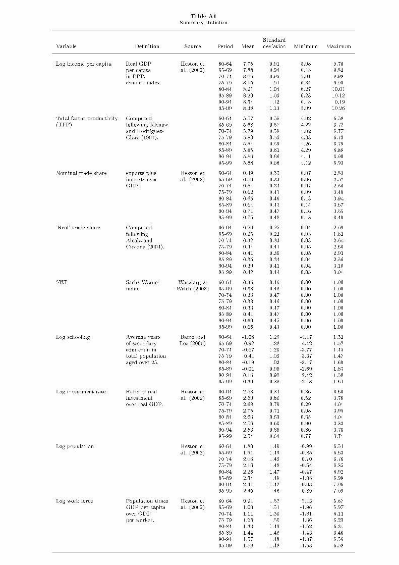
from speci…cation to speci…cation. Table A1 in the appendix provides the summary

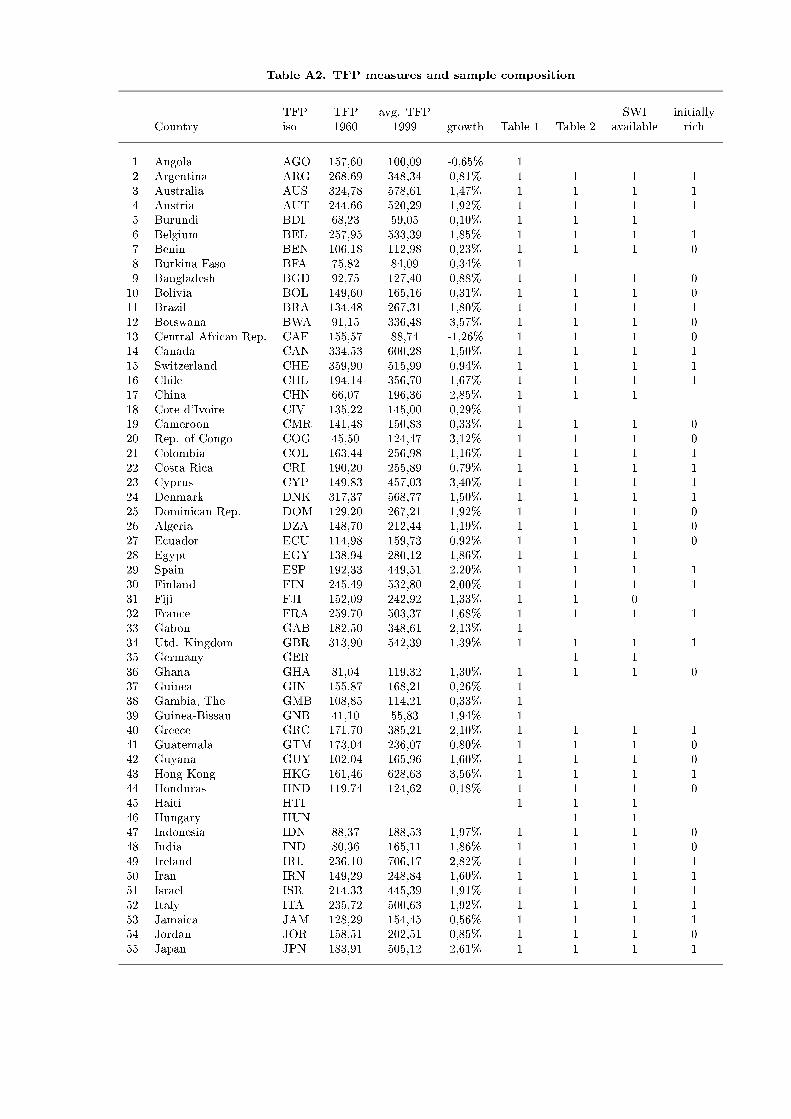
statistics for the data, Table A2 indicates the exact sample composition that underlies

the regressions.11

3.2 Measuring openness

Rodriguez and Rodrik (2001) distinguish between two broad measures of openness: a

…rst continuous measure that is directly related to actual trade ‡ows, and a second

binary one, which records whether a country is in principle open or not. We refer

to the …rst measure as revealed openness and distinguish between the nominal trade

share and a measure called real openness. The second type of measure, the well-known

Sachs-Warner index, captures political openness.

The measure of international trade used in almost all empirical work on the e¤ect on

trade on income or growth is nominal imports plus exports relative to nominal GDP,

usually referred to as openness or simply as the trade share. It has been used in a

large number of studies, from which the papers by Romer and Frankel (1999), Alesina

et al. (2000) and Irwin and Terviö (2002) may be the most well known. Alcalá and

Ciccone (2004) argue that in the context of cross-country productivity studies, there9This procedure has the drawback of wasting the available observations 1950-1960.

10From the OPEC members, only Algeria, Indonesia and Venezuela are in the sample. We conductsensitivity analysis to check whether those countries are important for the results.

11The data base used in the analysis can be obtained from the author at gfelberm@iue.it.

14

are sound theoretical reasons why this measure may result in a misleading picture of

the productivity gains due to trade. If trade increases productivity but these gains are

larger in the tradeable goods sector than in the non-tradeable goods sector, productivity

growth due to higher trade will not be necessarily associated with higher openness.

The reason is that the relatively greater productivity gains in manufacturing lead to

a rise in the relative price of services, which may result in a decrease in openness. To

remedy this problem, Alcalá and Ciccone propose a di¤erent measure that they call

real openness. Real openness is de…ned as imports plus exports in exchange rate US$

relative to GDP in purchasing power parity US$. Using real openness instead of the

nominal trade share as a measure of trade eliminates distortions due to cross-country

di¤erences in the relative price of non-tradeable goods. In the data, real openness is

obtained by multiplying openness by the price level. In the present paper, real openness

is the preferred index when we look at total factor productivity, and the nominal trade

share is preferred when we look at GDP per capita. With slight abuse of terminology,

we refer to Alcalá and Ciccone’s measure as to the ‘real’ trade share.

Another indicator for economic openness is the Sachs-Warner (1995) index (SWI).

The SWI is a binary variable that classi…es an economy as closed if one of the follow-

ing criteria is met: (i) the black market premium is larger than 20 percent, (ii) the

government has a purchasing monopoly on a major export crop and delinks purchase

prices from international prices, (iii) the country is socialist, (iv) own-import-weighted

average frequency of non-tari¤ measures (licenses, prohibitions, and quotas) on capital

goods and intermediates larger than 40 percent, and (v), the own-import-weighted av-

erage tari¤ on capital goods and intermediaries is greater than 40 percent. The SWI

indicator has been recently extended by Wacziarg and Welch (2003) and now covers a

longer time span and a larger number of countries.

Since the SWI index is a binary measure, it provides information on the degree of

trade-friendliness of a country’s institutions rather than on the importance of trade

15

as such. In cross-country regressions, it is therefore no wonder that introducing other

measures of institutional quality undoes the signi…cance of the Sachs-Warner index, as

other institutional variables are likely to be highly collinear to the SWI (Rodriguez and

Rodrik, 2001). Compared to the continuous openness index à la Frankel and Romer,

the SWI may have the advantage that its endogeneity to economic outcomes is less

problematic. In the paper, we use the SWI as an alternative measure of openness to

trade.

3.3 Construction of TFP measures

Growth accounting studies such as Hall and Jones (1999) show that cross-country

income di¤erences are to a large extent due to di¤erences in total factor productivity

(TFP). F&R do not …nd strong evidence for trade to a¤ect income through TFP. In

order to check this result in our more general framework, we need to construct an

appropriate TFP measure.

Following Klenow and Rodriguez-Clare (1997) as well as Benhabib and Spiegel

(2004), total factor productivity is estimated in the following way. Assuming that

initially all countries have been in their respective steady states, and using the simple

closed economy Solow model, initial capital stocks (as of 1960) of country i; Ki0; are

calculated according toKi0Yi0

=I=Yi

°i + ± + ni; (7)

where I=Yi is the average share of physical investment in output from 1960 to 2000,

°i represents the growth rate of output per capita over that period, ni is the average

growth rate of population and ± is a depreciation rate, assumed common to all countries,

and set equal to 0.03. Given initial capital stocks estimates, the capital stock of country

i in period t satis…es

Kit =tPj=0

(1 ¡ ±)t¡j Iij + (1 ¡ ±)tK0 for all t: (8)

16

Next, total factor productivity (TFP) is typically computed using a constant returns

to scale Cobb-Douglas production function with the capital share set to 1=3. For

country i at time t the log of TFP, ait can be written as

ait = yit ¡13kit ¡

23lit; (9)

where kit and lit denote the logarithms of the capital stock and the working population,

respectively. All the relevant data for this exercise come from the Penn World Tables

6.1. Working population has been constructed by computing the ratio between real

GDP per capita and real GDP per worker and then multiplying by population.12

Table A2 in the appendix shows the results for 102 countries. The results are almost

exactly identical to Benhabib and Spiegel, who have used the same data. As in their

analysis, a couple of countries have experienced negative TFP growth over the period.

With the exception of Venezuela, all these countries lie in subsaharan Africa. With the

exception of Nigeria, negative TFP growth is coupled with capital shallowing – i.e. a

negative growth rate of the K=L ratio. At the same time, on the other extreme of the

distribution, strong positive TFP growth goes hand in hand with capital deepening.

Most star performers in terms of TFP growth lie in south-east Asia, but there are

some noteworthy exceptions in subsaharan Africa: Botswana (BWA), the Republic of

Congo (COG) or Mauritius (MUS). Some exceptions notwithstanding, most countries

featuring a TFP growth rate larger than the US rate, have been able to close the gap

to the US.

The following section reviews F&R results and argues that their equation may be

seriously misspeci…ed. Consequentially, an explicitly dynamic estimation procedure is

needed.12Note, that the farther we move away from the initial starting point, the less important will the

(implausible) assumption be, that initially all economies have been in their respective steady states.

17

4 Revisiting Frankel and Romer (1999)

F&R estimate the causal e¤ect of changes in the nominal trade share on real per capita

income in the 1985 cross-section. The problem is that in most economic models, trade

and openness are both endogenous variables so that causal inference requires the use of

instruments. The contribution of F&R’s paper lies in the discovery of a clever instru-

ment for trade: …rst, they use bilateral trade data to estimate a gravity equation that

explains trade (exports plus imports) between country i and country j as a function

of geographical variables only (such as distance, the land area, population etc.), i.e.

deliberately omitting the income variables. Then, F&R retrieve the predicted bilateral

trade volumes and aggregate over j so as to construct total trade volumes for any

country i. In this way, they arrive at a measure of trade, which is by construction

orthogonal to income but still strongly correlated with the actual trade share and is

therefore a valid instrument. Their …ndings are (i) trade causes income, but the statis-

tical signi…cance of the e¤ect is ‘modest’, (ii) the OLS estimate seems to underestimate

the e¤ect of trade. Irwin and Terviö (2002) run the F&R model on historical data and

obtain results very similar to the ones found by F&R, in particular, IV estimates are

consistently larger than OLS estimates.

This section revisits F&R. It reproduces their baseline results for a slightly di¤erent

sample of countries and the up-to-date version of the Penn World Tables but uses

exactly the same instrument for the trade share. The estimates are almost identical

to those found by F&R. However, when initial GDP is added to the regression, the

regression turns out to perform better. In the standard F&R model, Rodriguez and

Rodrik (2000) have shown that the positive causal e¤ect of trade on income vanishes

once geographical latitude is added to the regression. Irwin and Terviö (2002) show

that this e¤ect does not depend on the particular subperiod under consideration.13

13Acemoglu et al. (2001) argue that latitude is itself a good proxy for institutional quality, becauseEuropean settlers chose to install good institutions only in those colonies where the climate was

18

This section shows, that geographical latitude does not destroy the causal e¤ect of

trade if a dynamic speci…cation is chosen. As a consequence, the dynamic speci…cation

may not only be desirable from a theoretical point of view, but may also improve the

robustness of the results.

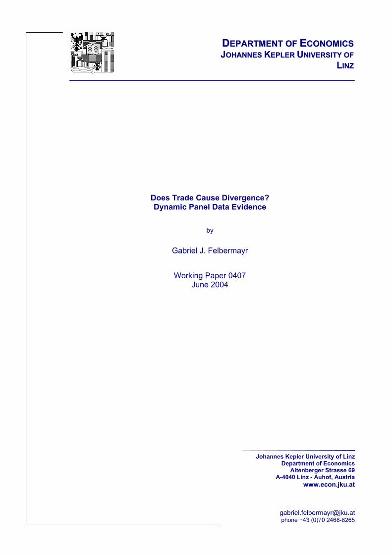
.2.4

.6.8

avg.

pol

itica

l ope

nnes

s (S

WI)

4050

6070

8090

avg.

reve

aled

ope

nnes

s

1950 1960 1970 1980 1990 2000year...

avg. revealed openness avg. political openness (SWI)

Source: Heston et al. (2002) and Wacziarg & Welch (2004).

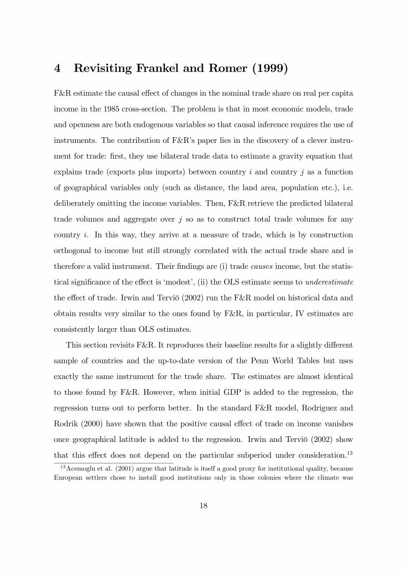
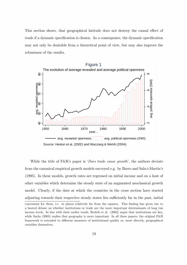
The evolution of average revealed and average political opennessFigure 1

While the title of F&R’s paper is ‘Does trade cause growth’, the authors deviate

from the canonical empirical growth models surveyed e.g. by Barro and Sala-ì-Martin’s

(1995). In these models, growth rates are regressed on initial income and on a host of

other variables which determine the steady state of an augmented neoclassical growth

model. Clearly, if the date at which the countries in the cross section have started

adjusting towards their respective steady states lies su¢ciently far in the past, initial

convenient for them, i.e. in places relatively far from the equator. This …nding has given rise toa heated debate on whether institutions or trade are the more important determinants of long runincome levels. In line with their earlier result, Rodrik et al. (2002) argue that institutions are key,while Sachs (2003) replies that geography is more important. In all these papers, the original F&Rframework is extended to di¤erent measures of institutional quality or, more directly, geographicalvariables themselves.

19

conditions should matter little in explaining current per capita real income. However,

the evolution of the world economy featured some important disruptions prior the date

(1985) at which F&R anchor their analysis and some of the shocks have occurred in the

global trading system. On its right axis, Figure 1 shows that in the last half-decade the

share of countries, classi…ed as open by the Sachs-Warner index has risen dramatically

from something slightly above 20% to 75%. Most of the increase has materialized after

1985, when many developing countries joined the global economy. Prior to that date,

the set of open countries more or less coincided with the group of OECD countries.

However, …gure 1 clouds the fact, that prior to 1985 many countries in the sample

switched from open to closed and vice versa, without there being a universal trend

towards more liberalization. In fact, Wacziarg and Welch (2004) identify 16 countries,

most of them in Central and South America, which experienced periods of temporary

liberalization between 1950 and 1985, some countries even switched their openness

status more than once. Hence, it would be wrong to conclude from Figure 1 that the

time span before 1985 was one where no trade-related shocks occurred.

Moreover, if one turns to the nominal trade share, it is clear that the time prior to

1985 was certainly not a period of tranquility. Average openness of countries peaked in

1980 after rising quite strongly, and then slided back again. The peak was due to the

strong rise in the price of oil, which in the short-run in‡ated the value of world trade.14

Typically, empirical estimates of the speed of conditional convergence are rather small

(Barro and Sala-ì-Martin, 1995) and lie between 2% and 3% (implying half-lives of

between 35 and 23 years). Moreover, many endogenous growth theories imply rather

small rates of convergence, too (see, e.g. Steger, 2003). Hence, it may be unrealistic to

assume that in 1985 countries have been even close to their respective steady states.15

It is then necessary, to cast the econometric model in a dynamic framework. Besides14The average ‘real’ trade share shows a similar pattern.15Mankiw et al. (1992) warn that the static model is “...valid only if countries are in their steady

states or if deviations from steady state are random”.

20

these principal considerations, allowing for conditional convergence in the formulation

of the model has important e¤ects on the results, as the next paragraphs try to show.

To see that the F&R model is probably misspeci…ed, we replicate their exercise with

our data, check Rodriguez and Rodrik’s (2000) critique, reformulate the econometric

framework as a standard cross-sectional growth model and check Rodriguez and Ro-

drik’s critique again. F&R run their regressions for a restricted sample of 98 countries,

for which they believe that data quality is higher. This data excludes oil-producing

countries and countries so small that their incomes are likely to be determined by idio-

syncratic factors. Our sample has 101 observations; the vast majority of which are also

present in F&R’s 98 countries sample. However, we do not use data from the Penn

World Tables 5.6. but from the corrected and updated version 6.1. Table A1 in the

appendix shows the exact list of countries covered.

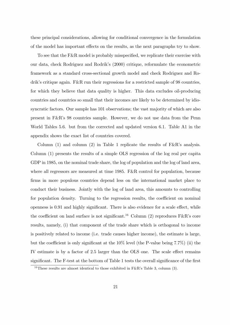
Column (1) and column (2) in Table 1 replicate the results of F&R’s analysis.

Column (1) presents the results of a simple OLS regression of the log real per capita

GDP in 1985, on the nominal trade share, the log of population and the log of land area,

where all regressors are measured at time 1985. F&R control for population, because

…rms in more populous countries depend less on the international market place to

conduct their business. Jointly with the log of land area, this amounts to controlling

for population density. Turning to the regression results, the coe¢cient on nominal

openness is 0.91 and highly signi…cant. There is also evidence for a scale e¤ect, while

the coe¢cient on land surface is not signi…cant.16 Column (2) reproduces F&R’s core

results, namely, (i) that component of the trade share which is orthogonal to income

is positively related to income (i.e. trade causes higher income), the estimate is large,

but the coe¢cient is only signi…cant at the 10% level (the P-value being 7.7%) (ii) the

IV estimate is by a factor of 2.5 larger than the OLS one. The scale e¤ect remains

signi…cant. The F-test at the bottom of Table 1 tests the overall signi…cance of the …rst16These results are almost identical to those exhibited in F&R’s Table 3, column (3).

21

stage regression, in which actual nominal openness is regressed on F&R’s constructed

trade share, on population and on land area. The results are not exactly identical to

those obtained by F&R (Table 3, column (4)), because the sample and the data are

slightly di¤erent. However, the estimated coe¢cients, the associated standard errors

and the R2 are very close.

While F&R’s framework has the advantage of parsimony, it is likely to su¤er from

omitted variables bias. In particular, institutional and geographical characteristics are

missing from the equation. Rodrik and Rodriguez (2000) add geographical latitude to

the model and …nd that the e¤ect of trade disappears. Column (3) shows what happens

if latitude is introduced into the regression. Now, the trade share is statistically not

distinguishable from zero and enters the equation with the wrong side. Strikingly,

income is rather well explained by a model that contains only latitude and a constant.

Both the F&R speci…cation and the R&R amendment assume that all countries in

the sample are on their balanced growth paths. To the extent that they are in the

process of convergence, the F&R and R&R equations are misspeci…ed. The remaining

columns of Table 2 show the results of prototype Barro-type growth regressions, where

equation (2) is estimated for two time observations only:

yi;1985 = ®+ °yi;1960 + ¿Ti;1985 +X0i;1985¯ + ui; i = 1; :::; N: (10)

The log of initial per capita income yi;1960 (1960) is added to the equation and the set

of controls now includes the log of years of schooling in 1960 to provide an additional

proxy for the steady state that the respective economies are converging to. Column

(4) provides a baseline OLS regression. Initial income and schooling enter with the

expected signs and magnitudes. Moreover, compared to the pure cross-section, the

Barro-type framework yields a precisely estimated trade coe¢cient which is much lower

than the one in Column (1). This is no surprise, since the coe¢cient in Column (1) is

not estimated consistently due to omitted variable bias. In the univariate case (where

the vector Xi is empty), the bias from omitting yi;0 is °cov(yi;0; Ti) =var(Ti) : Hence,

22

if initial income and trade in 1985 are positively correlated, and 0 < ° < 1 (as in

virtually all empirical growth studies) the bias is positive. In other words, it is not

high openness in the year of 1985 which is responsible for high income in 1985, but

the fact that the country was already rich to start with, which, in turn, is a function

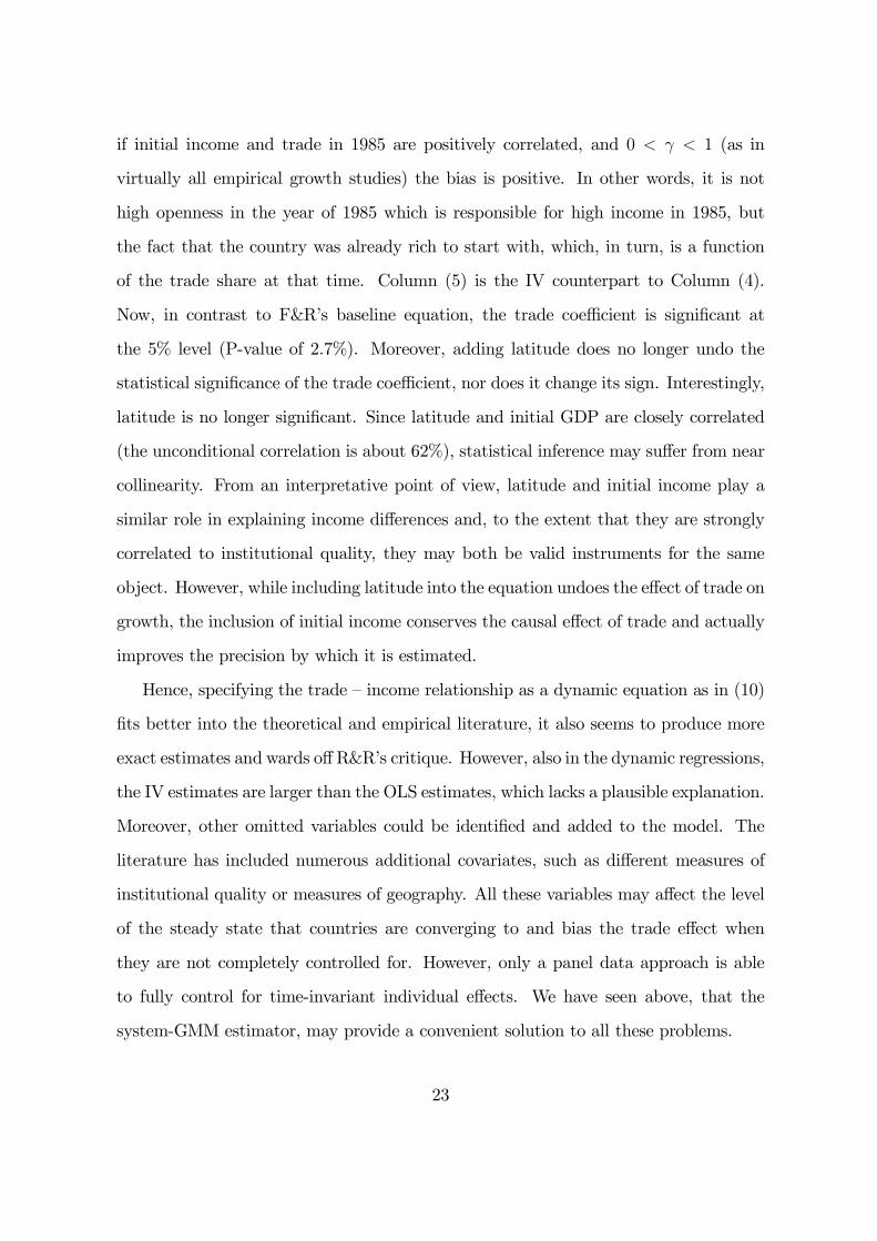
of the trade share at that time. Column (5) is the IV counterpart to Column (4).

Now, in contrast to F&R’s baseline equation, the trade coe¢cient is signi…cant at

the 5% level (P-value of 2.7%). Moreover, adding latitude does no longer undo the

statistical signi…cance of the trade coe¢cient, nor does it change its sign. Interestingly,

latitude is no longer signi…cant. Since latitude and initial GDP are closely correlated

(the unconditional correlation is about 62%), statistical inference may su¤er from near

collinearity. From an interpretative point of view, latitude and initial income play a

similar role in explaining income di¤erences and, to the extent that they are strongly

correlated to institutional quality, they may both be valid instruments for the same

object. However, while including latitude into the equation undoes the e¤ect of trade on

growth, the inclusion of initial income conserves the causal e¤ect of trade and actually

improves the precision by which it is estimated.

Hence, specifying the trade – income relationship as a dynamic equation as in (10)

…ts better into the theoretical and empirical literature, it also seems to produce more

exact estimates and wards o¤ R&R’s critique. However, also in the dynamic regressions,

the IV estimates are larger than the OLS estimates, which lacks a plausible explanation.

Moreover, other omitted variables could be identi…ed and added to the model. The

literature has included numerous additional covariates, such as di¤erent measures of

institutional quality or measures of geography. All these variables may a¤ect the level

of the steady state that countries are converging to and bias the trade e¤ect when

they are not completely controlled for. However, only a panel data approach is able

to fully control for time-invariant individual e¤ects. We have seen above, that the

system-GMM estimator, may provide a convenient solution to all these problems.

23

5 Results from a consistent dynamic panel data ap-proach

5.1 The e¤ect of instrumentation and the baseline model

In this section, we review the income-openness relationship when a GMM-type instru-

mentation strategy is chosen instead of the F&R instrument. Equation (2) is estimated

using di¤erent panel data techniques, with the system-GMM estimator being the pre-

ferred method. The aim of the analysis is to see (i) whether there is a robust positive

causal e¤ect of trade on income when other instruments are used and all time-invariant

country-speci…c …xed e¤ects are accounted for, and (ii) whether instrumenting increases

the coe¢cient of revealed openness relative to the uninstrumented case.

We address point (ii) …rst and show that using GMM-type instruments does not

lead to the kind of counterintuitive results as in F&R. The fact that the IV estimates

exceed the OLS estimates by a large amount is surprising and in contradiction with

economic theory. Normally one would expect that richer countries trade more because

they are rich: high-income countries have better infrastructure which facilitates trade,

demand for tradeable goods may rise faster than demand for nontradeables as countries

grow rich and poor countries may have little choice other than to resort to trade taxes

to …nance government spending, which would tend to depress openness. Hence, in an

OLS regression, trade and the error term should be positively correlated so that the

estimate would be biased upwards.17

In principle, F&R’s …nding may be triggered by sampling error, i.e. that the in-

strument is by pure chance positively correlated with the residual leading to a bias in

the IV results,. and / or by measurement error. Irwin and Terviö (2002) use F&R’s

instrument on a historical data set and …nd again that IV estimates are larger than the17There are arguments in trade theory (e.g. in the dynamic Heckscher-Ohlin model), why countries

may trade less when they grow richer (and in that model, more similar). However, these models aregenerally not corroborated by the data.

24

OLS ones. Hence, it is unlikely, that the wrong sign of the bias is due to sampling er-

ror. Measurement error may be an alternative explanation, because it biases the OLS

estimates downwards and instrumentation is the appropriate way to cure this prob-

lem. F&R argue that nominal openness ... “is only a noisy proxy for the many ways

in which interactions between countries raise income – specialization, spread of ideas,

and so on.” (F&R, p. 393) For example, openness may induce productivity-enhancing

technology spillovers that are not so much related to the volume of trade but rather to

the existence of an open trade relation between two countries. Similarly, trade theory

predicts that one major source for gains from trade resides in the dilution of market

power; again this e¤ect does not require actual trade ‡ows but depends on a credible

threat of entry (contingent markets). Hence, while the endogeneity bias leads OLS to

overestimate, measurement error leads to underestimation so that the sign of the bias

in the OLS estimates is ambiguous and may well be negative if measurement error is

large enough. However, as F&R admit, measurement error must be implausibly large

to overcompensate the endogeneity bias.

A conclusion of all these considerations is that the literature has not come up with

a convincing explanation of F&R’s results yet. One aim of the present study is to check

whether this anomaly persists when a di¤erent instrumentation strategy is chosen and

of country-speci…c …xed e¤ects are controlled for.

Table 2 reports di¤erent panel data estimates for (2). Data is available for a total

of 93 countries, see Table A2 for details. The panel is almost balanced: from the eight

…ve-years intervals available between 1960 and 1999, the …rst interval is lost due to

di¤erentiation of log income; the average number of observations per country is 6.78

which is very close to the maximum of 7. In all regressions reported in Table 2, lagged

income, schooling and investment are instrumented by their …rst order lags. In even

numbered columns, also the trade share is instrumented. This allows to isolate the size

and sign of the endogeneity bias which arises when the endogenous character of the

25

trade share is not appropriately addressed.

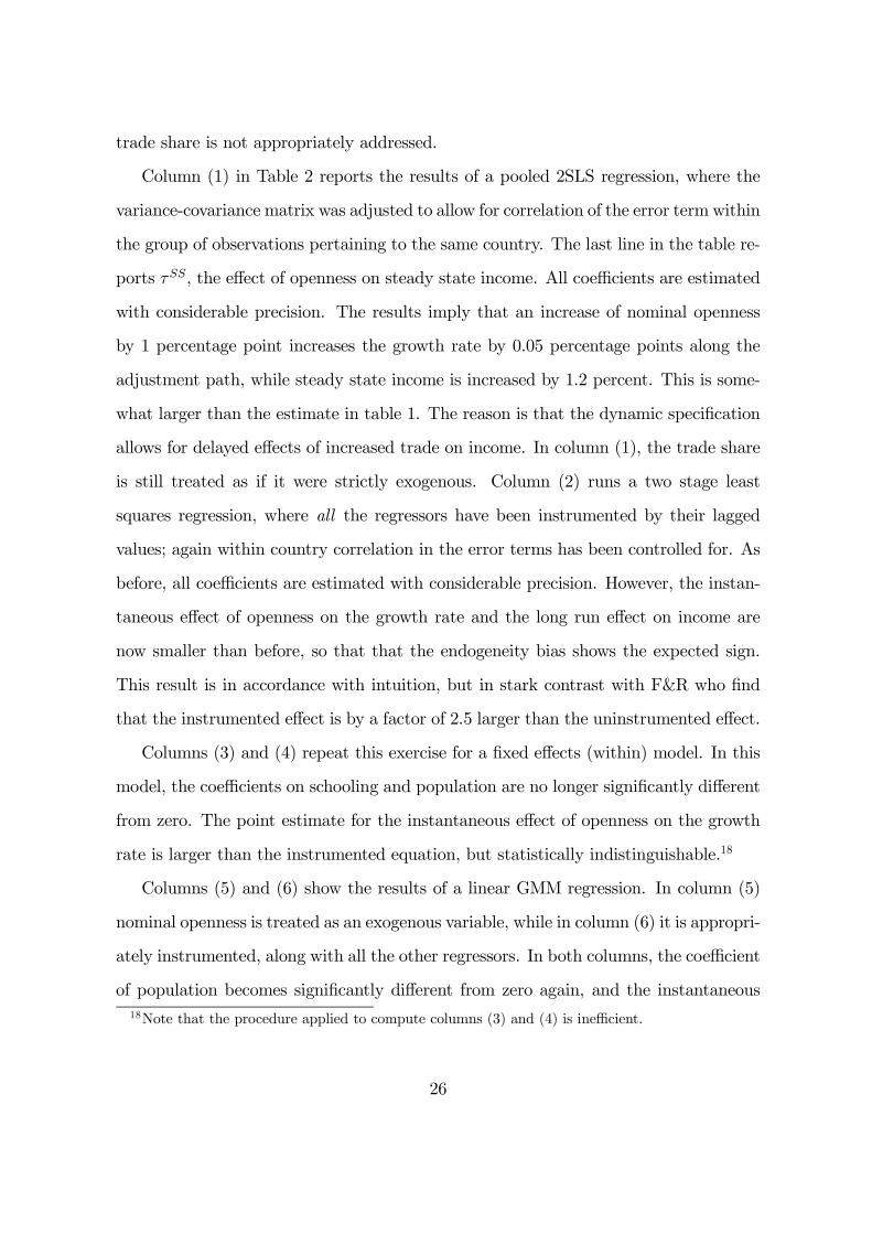
Column (1) in Table 2 reports the results of a pooled 2SLS regression, where the

variance-covariance matrix was adjusted to allow for correlation of the error term within

the group of observations pertaining to the same country. The last line in the table re-

ports ¿SS; the e¤ect of openness on steady state income. All coe¢cients are estimated

with considerable precision. The results imply that an increase of nominal openness

by 1 percentage point increases the growth rate by 0.05 percentage points along the

adjustment path, while steady state income is increased by 1.2 percent. This is some-

what larger than the estimate in table 1. The reason is that the dynamic speci…cation

allows for delayed e¤ects of increased trade on income. In column (1), the trade share

is still treated as if it were strictly exogenous. Column (2) runs a two stage least

squares regression, where all the regressors have been instrumented by their lagged

values; again within country correlation in the error terms has been controlled for. As

before, all coe¢cients are estimated with considerable precision. However, the instan-

taneous e¤ect of openness on the growth rate and the long run e¤ect on income are

now smaller than before, so that that the endogeneity bias shows the expected sign.

This result is in accordance with intuition, but in stark contrast with F&R who …nd

that the instrumented e¤ect is by a factor of 2.5 larger than the uninstrumented e¤ect.

Columns (3) and (4) repeat this exercise for a …xed e¤ects (within) model. In this

model, the coe¢cients on schooling and population are no longer signi…cantly di¤erent

from zero. The point estimate for the instantaneous e¤ect of openness on the growth

rate is larger than the instrumented equation, but statistically indistinguishable.18

Columns (5) and (6) show the results of a linear GMM regression. In column (5)

nominal openness is treated as an exogenous variable, while in column (6) it is appropri-

ately instrumented, along with all the other regressors. In both columns, the coe¢cient

of population becomes signi…cantly di¤erent from zero again, and the instantaneous18Note that the procedure applied to compute columns (3) and (4) is ine¢cient.

26

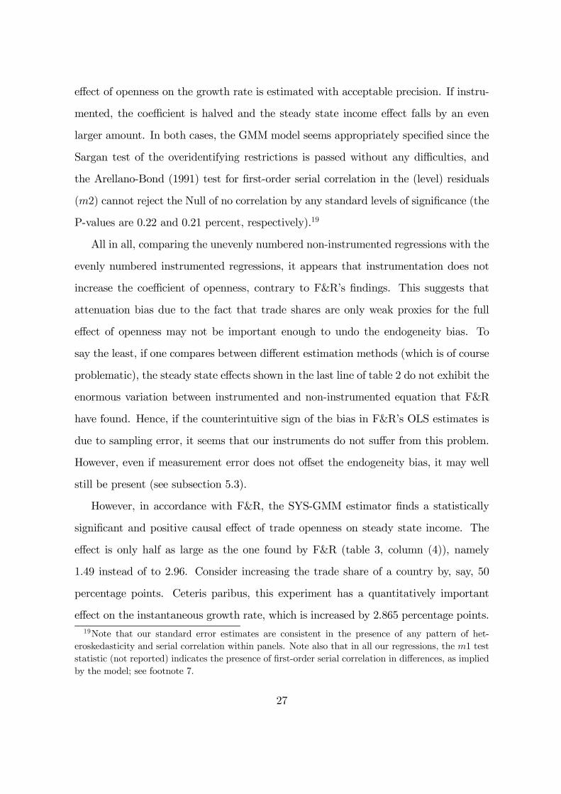
e¤ect of openness on the growth rate is estimated with acceptable precision. If instru-

mented, the coe¢cient is halved and the steady state income e¤ect falls by an even

larger amount. In both cases, the GMM model seems appropriately speci…ed since the

Sargan test of the overidentifying restrictions is passed without any di¢culties, and

the Arellano-Bond (1991) test for …rst-order serial correlation in the (level) residuals

(m2) cannot reject the Null of no correlation by any standard levels of signi…cance (the

P-values are 0.22 and 0.21 percent, respectively).19

All in all, comparing the unevenly numbered non-instrumented regressions with the

evenly numbered instrumented regressions, it appears that instrumentation does not

increase the coe¢cient of openness, contrary to F&R’s …ndings. This suggests that

attenuation bias due to the fact that trade shares are only weak proxies for the full

e¤ect of openness may not be important enough to undo the endogeneity bias. To

say the least, if one compares between di¤erent estimation methods (which is of course

problematic), the steady state e¤ects shown in the last line of table 2 do not exhibit the

enormous variation between instrumented and non-instrumented equation that F&R

have found. Hence, if the counterintuitive sign of the bias in F&R’s OLS estimates is

due to sampling error, it seems that our instruments do not su¤er from this problem.

However, even if measurement error does not o¤set the endogeneity bias, it may well

still be present (see subsection 5.3).

However, in accordance with F&R, the SYS-GMM estimator …nds a statistically

signi…cant and positive causal e¤ect of trade openness on steady state income. The

e¤ect is only half as large as the one found by F&R (table 3, column (4)), namely

1.49 instead of to 2.96. Consider increasing the trade share of a country by, say, 50

percentage points. Ceteris paribus, this experiment has a quantitatively important

e¤ect on the instantaneous growth rate, which is increased by 2.865 percentage points.19Note that our standard error estimates are consistent in the presence of any pattern of het-

eroskedasticity and serial correlation within panels. Note also that in all our regressions, the m1 teststatistic (not reported) indicates the presence of …rst-order serial correlation in di¤erences, as impliedby the model; see footnote 7.

27

Comparing the long-run equilibrium before and after the increase in openness shows

that the experiment boosts steady state income by 74.42%, which is again a very

considerable number. However, compared to F&R, this e¤ect is still small, since they

…nd that income would rise by 148%. Note that the e¤ect obtained with SYS-GMM is

quantitatively very similar to the one found in the 1985 cross section. Thus, it seems

that the largest part of the di¤erence between F&R’s results and the SYS-GMM results

come from choosing a dynamic speci…cation, rather than a static one. In contrast to

other methods, the GMM estimator makes sure that all time-invariant country-speci…c

…xed e¤ects are controlled for, that the lagged income variable on the right-hand-side of

the regression is appropriately dealt with and that all potentially endogenous regressors

are instrumented in a meaningful way.

The regression yields quantitatively plausible and statistically signi…cant coe¢cients

for all regressors. Most importantly, there seems to be evidence for a scale e¤ect since

the coe¢cient of population is positive and signi…cant. This is in line with F&R and

Alcalà and Ciccone.

Moreover, the regression in our Table 2, column (6), uses more than six times as

many observations than F&R. Hence, it seems safe to argue that the true causal e¤ect

from trade to income is smaller than what F&R claim. For the remainder of the paper,

the model reported in column (6) serves as the benchmark.

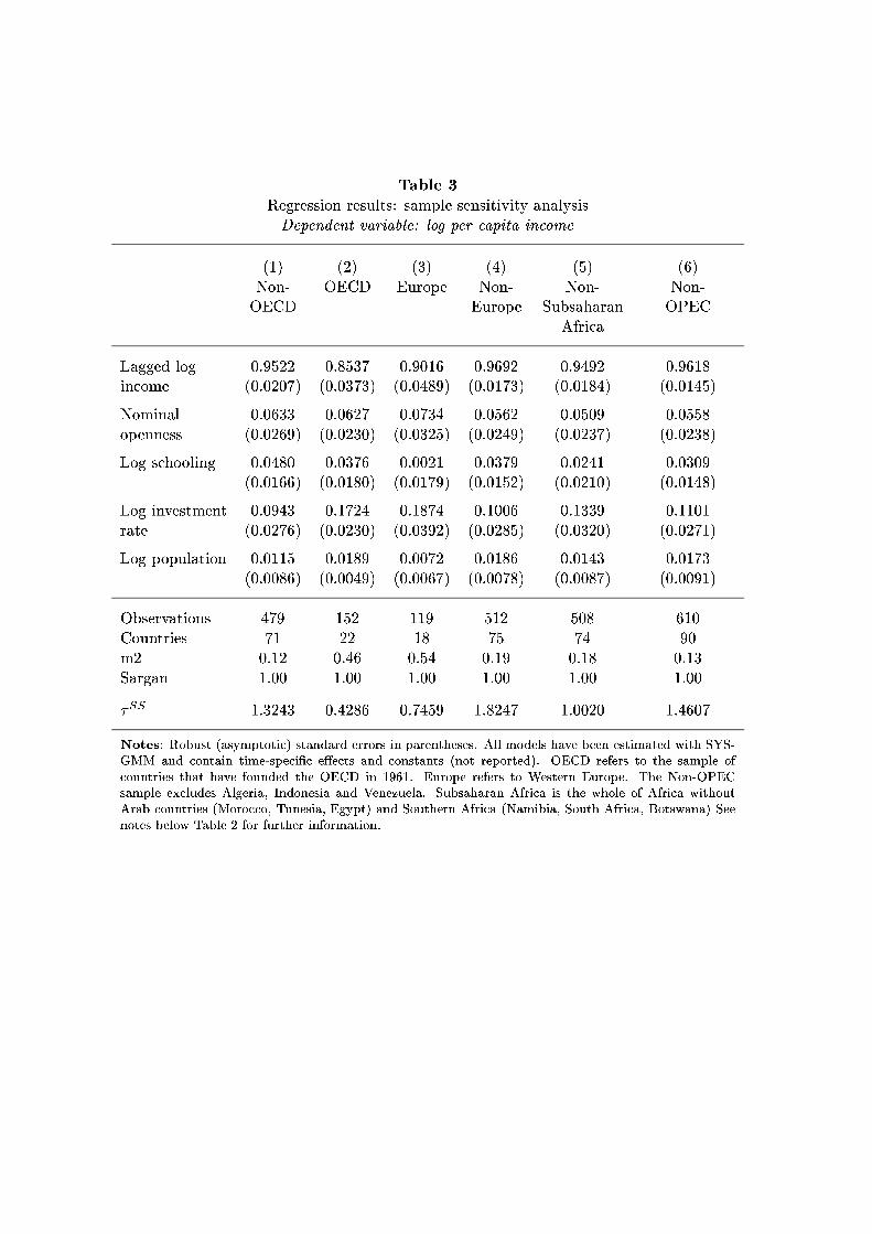
5.2 Sample sensitivity checks

Table 3 reports a number of sensitivity checks. Column (1) includes only non-OECD

countries while column (1) focuses on the much smaller subsample of OECD countries.20

Strikingly, the rate of conditional convergence in the OECD subsample is much larger

than in the non-OECD subsample (3% versus 1%, respectively), while the instanta-20To avoid the problem of endogenous sample selection, the OECD subsample includes only those

countries that have been members from the start (1961). This leaves us with the former EU15 (withoutLuxemburg), plus Switzerland, Norway, Turkey, Canada, USA, New Zealand, Australia and Japan.

28

neous e¤ect of an increase in nominal openness is almost the same in both subsamples.

This implies that the steady-state e¤ect is considerably larger in the non-OECD sam-

ple. Interestingly, the same observation can be made also with respect to schooling

and (albeit to a smaller extent) with respect to the investment rate.

Next we segment the sample into a European subsample (which is of course a

subset of the OECD sample), and a non-European subsample.21 Columns (3) and (4)

show that the coe¢cient on openness is statistically signi…cant and positive in both

the European and the non-European subsample, with the instantaneous e¤ect larger

and the long-run e¤ect smaller in the European subsample. Interestingly, there is no

evidence for a scale e¤ect in the European subsample, while size still matters in the

somewhat larger OECD subsample. This fact may be interpreted as evidence for the

European integration process, which makes the size of the home market more and more

irrelevant.

Column (5) excludes subsaharan Africa from the sample. Compared to the bench-

mark model, the instantaneous and the long-run e¤ects of openness change only slightly

and keep their statistical signi…cance. Thus, excluding low growth / low openness coun-

tries from the sample does not undo the results. However, excluding subsaharan Africa

undoes the signi…cance of the scale e¤ect. Hence, it seems that we …nd a positive scale

e¤ect in the full sample only because of the presence of those relatively closed African

countries whose growth perspectives are hampered by very limited home markets.

Column (6) excludes the three OPEC countries that are present in the full sample

(Algeria, Indonesia and Venezuela). Compared to the benchmark results, this exclusion

leaves all coe¢cients virtually unchanged.21The European sample comprises the former group of EU15 countries without Luxemburg, plus

Cyprus, Switzerland, Norway and Turkey.

29

5.3 Political versus revealed openness

In order to see what the nominal openness index really measures, it may be useful to

isolate the e¤ects of physical shipment of goods and services from those generated by

political openness. As stressed above, many bene…ts of openness do not need actual

trade ‡ows to materialize. Table 4 includes the Sachs-Warner Index (SWI) into the

econometric analysis. For comparison reasons, column (1) reproduces the baseline

result obtained in Table 4, column (6). Column (1) replaces the nominal openness

measure by the SWI. While an increase of the trade share by one percentage point

causes an instantaneous growth e¤ect of about 0.06 percentage points, switching from

being closed to being open causes growth to shoot up by 6.66 percentage points. This

is equivalent to increasing the trade share by 110 percentage points.

Column (3) runs a regression in which both the nominal trade share and the SWI are

present. Strikingly, now the trade share is no longer signi…cant while the SWI coe¢cient

and the associates standard error change only slightly with respect to column (2). If

one controls explicitly for political openness, there is no strong evidence that increasing

the trade share boosts income. Hence, it appears that the bene…cial e¤ects from trade

do not come from the physical delivery of goods as such but more from the general fact

that a country is open and participates in the international economy.

The message of including the SWI index is twofold. First, there is a causal e¤ect

of openness on instantaneous growth regardless of the exact de…nition of openness.

Second, the trade share may indeed be a noisy proxy for openness. This implies that

the pure endogeneity bias is probably larger than what the results in Table 2 suggest.

5.4 Do initially poor countries bene…t less from globalization?

Now, we take up the politically interesting question whether initially poor countries

bene…t from globalization on equal terms than initially rich countries. To check this

question, we divide our sample into two subsamples: of initially ‘rich’ and one of

30

initially ‘poor’ countries. Poor countries are those whose log income per capita in

1960 was smaller than the median level, the subsample of rich countries is just the

remainder. In order to provide a check on whether our results depend on this particular

segmentation of the data, we work with a second de…nition, whereby a country is poor

if its log income per capita in 1960 was smaller than the 25% percentile and rich

otherwise. Only countries for which per capita income is observed in 1960 are in the

sample, hence our panel is perfectly balanced. Table A2 in the appendix informs which

countries are in the sample and which are classi…ed as rich or poor according to our

…rst segmentation.

Table 5 compares the median growth rates measured in the sample as a whole and

in the two subsamples. It turns out that the median growth rate in the poor subsample

was substantially lower rates than that in the rich subsample or in the total sample.

While in the full sample, the median growth rate over the 1960-1999 period was 1.73%,

countries initially poorer than the median grew by a mere 0.80% and those poorer than

the 25%-percentile by an even smaller 0.70%.22

Is trade causally responsible for the lack of absolute convergence, as shown in Table

5, or must other factors be blamed? Our GMM panel approach is a good means to

answer this question, because it controls for all time-invariant country-speci…c e¤ects,

therefore isolating the e¤ect of trade. Denote the indicator of initial per capita GDP

by Ii1: Regardless of whether Ii1 is a binary or a continuous variable, the empirical

speci…cation now contains an interaction term

Tit ¤ Ii1:yit = °yi;t¡1 + ¿ 1Tit + ¿ 2 (Tit ¤ Ii1) +X0it¯ + ±t + (´i + Ii1) + vit: (11)

If ¿2 is strictly negative, the causal e¤ect of trade on growth is smaller for coun-

tries who feature a higher value of Ii1 and trade can be seen as a driving factor for

convergence.22Our measure of divergence probably overstates the true divergence; comparing means leads to

a less dramatic picture. However, while the extent of absolute divergence is disputable, there is noevidence in favor for convergence.

31

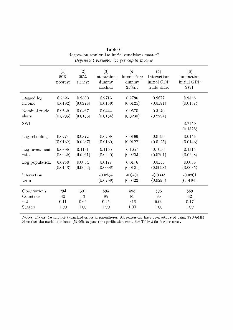
First, we run our baseline regression (2) separately for both subsamples. The results

are shown in columns (1) and (2) in Table 6. The instantaneous growth e¤ect of

openness appears larger for initially poor countries, albeit the e¤ect is imprecisely

estimated. However, there is evidence, that investment has a higher but shorter lived

e¤ect on the growth rate of initially rich countries. Running two separate regressions

exploits only variation within the two subsamples. Hence, we can only conclude that

compared to the other countries in the same group, openness pays o¤ more in the sample

of poor countries. However, it may well be that, as a group, poor countries bene…t

much less from openness than rich countries. To allow for both, within group variation

and between group variation, column (3) adds the interaction term to the regression.

To start with, I1i is a dummy variable that takes the value of one if the country is in

the subsample of initially rich countries and the value of zero if it is in the subsample of

initially poor ones. This allows group speci…c variation in the coe¢cient of openness,

but constrains the other coe¢cients to be identical across groups. It turns out that the

interaction term has a negative sign but is statistically not di¤erent from zero. Hence,

we do not …nd any systematic evidence, that openness causally a¤ects initially poor

countries di¤erently than initially rich ones. The pattern of divergence that emerged

from Table 5 cannot be attributed to trade openness and must be due to some di¤erent

factor. To explain divergence, one would have to turn towards the country-speci…c

…xed-e¤ects which capture institutional and geographical characteristics.

The remaining columns show the results of some robustness checks. In column (4),

the variable Ii1 is still a binary one, and takes the value of one if a country had a 1960

log income per capita larger than the 25%-percentile and the value of zero otherwise.

Again trade does not turn out to be causally responsible for the poor performance of

those countries that in 1960 counted amongst the 25% poorest.

In column (5), Ii1 is just the initial log of per capita income. In contrast to the

cases discussed before, this regression does not pass the speci…cation test m2, the null

32

of serial correlation in the error terms cannot be rejected at the 10% signi…cance level.

However, this problem notwithstanding, initial income does not appear to matter for

the causal e¤ect of trade on income and the result is qualitatively similar to the earlier

regressions.

Finally, column (6) checks whether the insensitivity of the trade e¤ect with respect

to initial GDP depends on the precise de…nition of openness. When the trade share is

replaced by the Sachs-Warner index, the picture does not change qualitatively: again,

there is no evidence that the interaction of initial income with the SWI index plays

any role in determining growth.

Hence, to say the least, if backwardness is not a virtue, as column may (1) suggest,

it certainly does not appear to be a handicap and the causal e¤ect of trade on growth

is not di¤erent for initially poor countries.

5.5 On the role of TFP in the growth-openness nexus

Table 6 reproduces our results if log TFP is used as the dependent variable. Following

Alcalà and Ciccone (2004), real openness is used to measure the importance of trade.

Moreover, instead of population the regression controls for the size of the working force.

Column (1) shows the results of a baseline regression, which is perfectly analogous

to the one run for capita real income. However, in line with F&R’s results, we do

not …nd much evidence for a positive causal e¤ect of trade on TFP. The estimated

coe¢cient is much smaller than when per capita real income is used as the dependent

variable and it is very imprecisely estimated. Schooling does not seem to be causally

related to TFP, while the investment rate turns out to be rather important. The

only interesting …nding in column (1) is that of statistically signi…cant adjustment

dynamics. While this is a common …nding in GDP regressions, there is less evidence in

the literature for conditional convergence in TFP. Moreover, there may be a positive

scale e¤ect: increasing the work force has a (weakly) signi…cant positive e¤ect on the

33

instantaneous growth rate of TFP and the long-run TFP level. However, the results

must be interpreted with caution, because the Arellano-Bond test (m2 ) for second

order serial correlation in the residuals almost rejects the null of no serial correlation

(the P-value is 9%).

Column (2) repeats the analysis but uses the SWI dummy instead of the real trade

share as a measure of openness. The m2 -measure is somewhat more supportive, but

besides the investment rate (and lagged TFP) we do not identify any other causal

e¤ects of openness on the growth rate of TFP. Column (3) puts the real trade share

together with the SWI into the regression. This alters the results exhibited in column

(2) only very slightly.

Now come more interesting results: if the sample is restricted to the 50% countries

with the lowest 1960 TFP level, we …nd a quantitatively important and statistically

signi…cant causal e¤ect of trade on the instantaneous growth rate. In contrast, focussing

on the 50% countries with the highest 1960 TFP level, we fail to identify such an e¤ect.

Column (6) again considers the full sample and checks the interaction poor¤open where

poor is a dummy that takes the value of unity if the country had a 1960 TFP level

below that of the median. Hence, while there was no evidence either for an advantage

or a handicap of backwardness in the GDP regressions, now we are led to conclude

that in terms of total factor productivity, initially less productive countries tend to

bene…t more from an increase in trade. This result has been checked for its robustness

by considering other de…nitions of the group of initially poor countries. However, the

result remains robust.

6 Conclusions

The present paper revisits the empirical relationship between trade and growth in a

panel of countries, using the system-GMM estimator proposed by Blundell and Bond

(1998). This method has the advantage that it allows consistent estimation even if the

34

growth model is speci…ed as a dynamic AR(1) relationship and all the right-hand-side

variables are potentially endogenous and/or prone to measurement error. Moreover,

through …rst-di¤erencing, the procedure o¤ers a natural way to control for institutional

and geographical characteristics as long as they are time-invariant.

The paper …rst argues that the widely cited model by Frankel and Romer (1999)

may be misspeci…ed, because it makes the implicit assumption that all countries are in

their respective steady states. Since the globalization is a rather recent phenomenon,

this seems a questionable requirement. If F&R’s model is reformulated to allow for

adjustment dynamics, the causal e¤ect of trade on growth is estimated more precisely

than in a static framework. Moreover, inclusion of geographical latitude (distance from

the equator) no longer destroys the e¤ect.

F&R’s main contribution was the suggestion of a clever instrument to account

for the endogeneity of the trade share in the trade-growth relationship. However,

they found that the estimate obtained under 2SLS is much larger than the one found

using OLS. This runs against intuition and theoretical reasoning. Using a GMM-type

instrumentation strategy, the present paper …nds that the e¤ect of instrumented trade

is not larger than the uninstrumented one, con…rming the hypothesis that income is

positively associated with trade.

Next, the empirical relationship between trade and growth is estimated using the

system-GMM estimator. It turns out that the more general econometric approach

con…rms F&R’s …nding of a robust and positive causal e¤ect of trade on growth. This

result is found after controlling for country-speci…c …xed-e¤ects, the endogeneity of all

regressors and the presence of a lagged dependent variable on the right-hand-side of

the equation. The model passes a variety of sensitivity checks, suggesting that the

positive trade–growth relationship is rather robust.

Finally, the empirical model is used to check whether trade is causally responsible

for the failure of initially poor countries to catch up with the richer ones. There is little

35

evidence that the trade share has a di¤erent e¤ect for initially poor countries; the point

estimates within the subsample of poor countries and the sign of the interaction e¤ect

actually suggest the contrary, albeit without satisfactory precision. However, when the

model is used to investigate the e¤ect of trade on total factor productivity growth, we

…nd fairly robust evidence that trade is actually more bene…cial for countries that start

with a lower level of TFP.

The system-GMM procedure employed in the present paper is not a panacea. It

has two major drawbacks: …rst, to the extent that institutional features of countries

are time-variant, they are not controlled for; second, the empirical framework accounts

for endogenous growth only by including the time dummies ±t: The …rst problem may

be resolvable as time passes on. At the moment, the time series of institutional quality

indicators, as published by the World Bank or elsewhere, do not cover any extensive

period of time and are therefore of little use in a dynamic panel data framework. The

second problem appears in any stationary econometric model. Its resolution would

require a framework that allows for country-speci…c long-run time e¤ects.

36

References

[1] Acemoglu, Daron, Simon Johnson and James A. Robinson. 2001. ‘The Colonial

Origins of Comparative Development: An Empirical Investigation.’ American Eco-

nomic Review 91(5), 1369-1401.

[2] Acemoglu, Daron and Jaume Ventura. 2002. ‘The World Income Distribution’.

Quarterly Journal of Economics 117(2), 659-94.

[3] Alcalá, Francisco and Antonio Ciccone. 2004. ‘Trade and Productivity’. Quarterly

Journal of Economics 119(2), 613-646.

[4] Alesina, Alberto, Enrico Spoalore and Romain Wacziarg. 2000. ‘Economic Integra-

tion and Political Desintegration.’ American Economic Review 90(2), 1276-1296.

[5] Arellano, Manuel and Bond, Stephen R. 1991. ‘Some Tests of Speci…cation for

Panel Data: Monte Carlo Evidence and an Application to Employment Equations.’

Review of Economic Studies 58(2), 277-297.

[6] Barro, Robert J. and Jong-Wha Lee. 1996. ‘International Measures of Schooling

Years and Schooling Quality.’ American Economic Review 86(2), 218-223.

[7] Barro, Robert J. and Jong-Wha Lee. 2000. ‘International Data on Educational

Attainment: Updates and Implications’. CID Working Paper 42.

[8] Barro, Robert J. and Xavier Sala-ì-Martin. 1995. Economic Growth. (Cambridge,

MA: MIT Press).

[9] Benhabib, Jess and M.M. Spiegel. 2000. ‘The Role of Financial Development In

Growth and Investment.’ Journal of Economic Growth 5(4), 341-360.

37

[10] Benhabib, Jess and M.M. Spiegel. 2004. ‘Human Capital and Technology Dif-

fusion.’ in: Philippe Aghion and Steven Durlauf (eds.), Handbook of Economic

Growth Ch. 22.

[11] Bond, Stephen R., Anke Hoe­er and Jonathan Temple. 2001. ‘GMM Estimation

of Empirical Growth Models’. CEPR Discussion Paper 3048.

[12] Blundell, Richard W. and Stephen, R. Bond. 2000. ‘GMM Estimation with Persis-

tent Panel Data: An Application to Production Functions’. Econometric Reviews

19(3), 321-340.

[13] Caselli, Francesco, Gerardo Esquivel and Fernando Lefort. 1996. ‘Reopening the

Convergence Debate: A New Look at Cross-country Growth Emprics’. Journal of

Economic Growth 1(3), 363-389.

[14] Dollar, David and Aart Kraay. 2003. ‘Institutions, Trade, and Growth’. Journal

of Monetary Economics 50(1), 133-162.

[15] Feenstra, Robert C. 2004. Advanced International Trade: Theory and Evidence.

(Princeton, NJ: Princeton University Press).

[16] Forbes, Kristin J.. 2000. ‘A Reassessment of the Relationship Between Inequality

and Growth’. American Economic Review 90(4), 869-887.

[17] Frankel, Je¤rey, and David Romer. 1999. ‘Does Trade Cause Growth’. American

Economic Review 89(3), 379-399.

[18] Gancia, Gino. 2003. ‘Globalization, Divergence and Stagnation’. Institute for In-

ternational Economic Studies Working Paper 720.

[19] Grossman and Helpman. 1991. Innovation and Growth in the Global Economy.

(Cambridge, MA: MIT Press).

38

[20] Hall, Robert E. and Charles I. Jones. 1999. ‘Why Do Some Countries Produce So

Much More Output Per Worker Than Others?’ Quarterly Journal of Economics

114(1), 83-116.

[21] Heston, Alan, Robert Summers and Bettina Aten. 2002. Penn World Table Ver-

sion 6.1. Center for International Comparisons at the University of Pennsylvania

(CICUP).

[22] Holtz-Eakin, Douglas, Whitney Newey and Harvey S. Rosen. 1988. ‘Estimating

Vector Autoregressions with Panel Data’. Econometrica 56(6), 1371-95.

[23] Islam, Nazrul. 1995. ‘Growth Empirics: A Panel Data Approach.’ The Quarterly

Journal of Economics 110(4), 1127-1170.

[24] Irwin, Douglas A. and Marko Terviö. 2002. ‘Does Trade Raise Income? Evidence

From the Twentieth Century.’ Journal of International Economics 58(1), 1-18.

[25] Klenow, Peter and Andres Rodriguez-Clare. 1997. ‘The Neoclassical Revival in

Growth Economics: Has It Gone Too Far’ in Ben S. Bernanke and Julio Rotem-

berg, eds., NBER Macroeconomics Annual 1997 (Cambridge, MA: MIT Press).

[26] Levine, Ross, Norman Loayza and Thorsten Beck. 2000. Financial Intermediation

and Growth: Causality and Causes. Journal of Monetary Economics 46(1), 31-77.

[27] Lucas, Robert E.. 1988. ‘On the Mechanics of Economic Development.’ Journal of

Monetary Economics 22(1), 3-42.

[28] Mankiw, Gregory, David Romer, and David Weil. 1992. ‘A contribution to the

Empirics of Economic Growth’. Quarterly Journal of Economics 107(2), 407-437.

[29] Nickel, Steven. 1981. ‘Biases in Dynamic Models Using Fixed E¤ects’. Economet-

rica 49(6), 1417-1426.

39

[30] Rodriguez, Francisco and Dani Rodrik. 2001. ‘Trade Policy and Economic Growth:

A Skeptic’s Guide to the Cross-National Evidence’ in Ben S. Bernanke and Ken-

neth Rogo¤, eds., NBER Macroeconomics Annual 2000 (Cambridge, MA: MIT

Press).

[31] Rodrik, Dani, Arvind Subramanian and Francesco Trebbi. 2003. ‘Institutions Rule:

The Primacy of Institutions Over Geography and Integration in Economic Devel-

opment’. mimeo: Harvard University.

[32] Sachs, Je¤rey D. and Andrew Warner. 1995. ‘Economic reform and the process of

global integration.’ Brookings Papers on Economic Activity 1995(1), 1-119.

[33] Sachs, Je¤rey D. 2003. ‘Institutions Don’t Rule: Direct E¤ects of Geography on

Per Capita Income’. NBER Working Paper 9490.

[34] Staiger, D. and J.H. Stock (1997). ‘Instrumental Variables Regression With Weak

Instruments’. Econometrica 65, 557-586.

[35] Steger, Thomas M. 2003. ‘The Segerstrom Model: Stability, Speed of Convergence

and Policy Implications.’ Economic Bulletin 15(4), 1-8,

[36] Stokey, Nancy. 1991. Human Capital, Product Quality, and Growth. Quarterly

Journal of Economics 106(2), 587-616.

[37] Young, Alwyn. 1991, Learning by Doing and the Dynamic E¤ects of International

Trade, Quarterly Journal of Economics 106(2), 369-405.

[38] Wacziarg, Romain T. and Karen Horn Welch. 2003. Trade Liberalization and

Growth: New Evidence. NBER Working Paper 10152.

40