Does the Stock Market Fully Appreciate the Implications of Leading Indicators for

Future Earnings? Evidence from Order Backlog

Shivaram Rajgopal Department of Accounting University of Washington

Box 353200 Seattle, WA 98195 Fax: 206 685 9392

E-mail: rajgopal@u.washington.edu

Terry Shevlin* Deloitte and Touche Professor

Department of Accounting University of Washington

Box 353200 Seattle, WA 98195 Tel: 206 543 7223 Fax: 206 685 9392

E-mail: shevlin@u.washington.edu

and

Mohan Venkatachalam Fuqua School of Business

Duke University P.O. Box 90120

Durham, NC 27708 Tel: 919 660 7859 Fax: 919 660 7971

Email: vmohan@duke.edu

June 11, 2003 *Contact author

Abstract. Although leading indicators are becoming increasingly important for equity

valuation, disclosures of such indicators suffer from the absence of GAAP related

guidance on content and presentation. We explicitly examine (i) whether one leading

indicator � order backlog � predicts future earnings, and (ii) whether market participants

correctly incorporate such predictive ability in determining share prices. We find that the

stock market overweights the contribution of order backlog in predicting future earnings,

and a hedge strategy that exploits such overweighting generates significant future

abnormal returns. However, such mispricing is not due to analysts� inability to

incorporate order backlog into their earnings forecasts.

Keywords: leading indicator, backlog, mispricing, market efficiency, analyst forecasts

JEL classification: M41, G14

1

In this study, we investigate whether capital market participants, i.e., investors and analysts,

incorporate the implications of one leading indicator � order backlog � for future earnings in an

efficient manner when determining stock prices and earnings forecasts. The market value of a

firm�s shares and analyst forecasts should reflect an unbiased expectation of future earnings. To

the extent current earnings persist in the future, the link between current and future earnings is

relatively apparent. However, in today�s dynamic business environment, a substantial portion of

future earnings may reflect the contribution of several leading indicators such as backlog (Behn,

1996), product market share (Amir and Lev, 1996), customer satisfaction (Ittner and Larcker,

1998a), patents (Deng, Lev, and Narin, 1999), web traffic (Trueman, Wong, and Zhang, 2001;

Rajgopal, Venkatachalam, and Kotha, 2003) or managerial actions (Rajgopal, Venkatachalam,

and Kotha, 2002). Under generally accepted U.S. accounting principles, such leading indicators

are not recognized but are often disclosed in the firm�s financial statements. When an

economically significant portion of a firm�s future earnings stems from leading indicators, the

absence of explicit information about the contribution of such indicators to future earnings

complicates the task of equity valuation.

Disclosure issues related to leading indicators have grown in importance in recent years.

One reason for such focus is claims about the declining importance of accounting-based

performance metrics such as earnings and equity book values (see Collins, Maydew, and Weiss,

1997; Francis and Schipper, 1999; Brown, Lo, and Lys, 1999; Lev and Zarowin, 1999). Further,

the Jenkins Committee report (AICPA, 1994) and research on the lead-lag relation between stock

prices and earnings (see Kothari, 2001) kindled an active interest among academics in

understanding whether leading indicators of future earnings could potentially remedy the

perceived fall in the value-relevance of earnings and book value. Several practitioners (e.g.,

2

Kaplan and Norton, 1996; Eccles et al., 2001) have called for a reporting framework that

integrates traditional financial measures and leading indicators. Recently, national regulators

such as the FASB (2001) and SEC (2001) and international regulators such as the Canadian

Institute of Chartered Accountants (1995) and Institute of Chartered Accountants of England and

Wales (2000) have published studies that discuss the possibility of mandating enhanced

disclosures of leading indicators.

The increased importance of non-GAAP leading indicators raises the question of whether

security prices reflect their unbiased contribution to future earnings. In an efficient market, the

stock market correctly impounds the value of a leading indicator for future earnings. Hence,

there ought to be no association between leading indictors and future stock returns. On the other

hand, several characteristics of these leading indicators impede a clear understanding of their

implications for future earnings. Most leading indicators are inherently idiosyncratic to specific

industries and some are even specific to individual firms. Disclosure of such metrics is voluntary

and is open to management discretion. Furthermore, the content and presentation of such

disclosures are not standardized by GAAP. Many indicators are not denominated in dollars,

rendering cross-firm comparison of such indicators difficult. Moreover, a recent FASB study

(FASB 2001) found several problems in the extant disclosures: (i) indicators were presented in

isolation without relating them to the context of the industry and the company; (ii) the

measurement and presentation of some indicators were not consistent over time; (iii) some firms

presented vague metrics such as �organization enhancing customers� or �image enhancing

customers� without a concise definition of the metric or its measurement.

These complications raise the possibility that stock prices do not fully incorporate the

contribution of leading indicators for future earnings. On account of uncertainty inherent in

3

translating leading indicators to value creation, investors may excessively discount the

contribution of such indicators to future earnings. Underpricing may also arise if investors are

functionally fixated on current earnings -- i.e., they mechanically accept firms� current earnings

numbers at face value without adjusting for the long-term benefits of the underlying activities or

processes captured by leading indicators.

In contrast, some observers have suggested that investors overestimate the benefits from

leading indicators, especially in hot sectors of the economy such as Internet-intensive businesses

or the wireless industry (Damodaran, 2001; D�Avolio, Gildor, and Shleifer, 2001). There is wide

coverage of leading indicators such as POPS (population coverage), book-to-bill ratio or

customer satisfaction indices in the media and some firms devote intensive marketing efforts to

promote such indicators. As a result, the market may be overly optimistic about the contribution

of such indicators to future earnings. The objective of our study is to explicitly examine whether

investors appropriately account for the contribution of leading indicators to future earnings.

We choose order backlog as the leading indicator in our empirical tests because an

investigation into the potential mispricing of a widely disseminated, dollar denominated leading

indicator that is readily available and cross-sectionally comparable for a large number of firms

across several industries gives the null of market efficiency the best possible chance of success.

Moreover, order backlog is economically significant (30% of total assets for the median sample

firm) and is somewhat standardized in its definition and disclosure. If the market has difficulty

in interpreting the implications of order backlog for future earnings, it is more than likely that the

market fails to fully appreciate the implications of non-dollar denominated, less widely

disseminated, and less objective leading indicators such as customer satisfaction measures, web

4

traffic, patents or firm-or industry-specific metrics such as manufacturing cycle time or time-to-

market measures.

Our empirical tests use the Mishkin (1983) framework to examine whether market

participants incorporate into stock prices the predictive ability of order backlog for future

earnings. The results indicate that the stock market behaves as if backlog contributes more to

future earnings than is implied by the cross-sectional association between backlog and future

earnings. To corroborate findings from the Mishkin (1983) test, we assess whether abnormal

future returns can be earned by taking positions on current order backlog. We find that a Fama

and MacBeth (1973) type hedge strategy based on taking positions on order backlog can earn

abnormal returns of 7.7% as compared to 16.6% abnormal returns that can be earned from

Sloan�s (1996) accrual-based anomaly. Moreover, abnormal returns based on order backlog are

robust to the inclusion of Fama and French (1992) risk factors and are incremental to abnormal

returns earned from Sloan�s (1996) accrual anomaly.

Next, we examine whether the failure of equity investors to correctly incorporate the

implications of order backlog for future earnings is at least partially explained by the failure of

sophisticated information intermediaries, such as equity analysts, to incorporate the contribution

of backlog to future earnings when generating earnings forecasts. Our results suggest otherwise;

we find that median consensus analysts� forecasts correctly incorporate the information

contained in backlog for future earnings. Finally, we find that even after controlling for

information in analysts forecasts for future earnings, investors continue to place weight on order

backlog information. This result is consistent with market participants not appreciating the fact

that analyst forecasts already incorporate information in order backlog.

5

Our study extends two areas of prior research. First, we contribute to the literature that

documents a relation between stock prices and leading indicators. The association between

leading indicators and stock prices is usually taken as evidence that the market correctly prices

the contribution of such leading indicators to future earnings. However, recent research raises

doubts about that assumption. In particular, survey evidence presented by Ittner and Larcker

(1998b) suggests that even managers question the quality of leading indicator information.

Furthermore, a field study conducted by Banker, Potter, and Srinivasan (2000) indicates that

managers, let alone investors, cannot fully articulate the link between leading indicators and firm

value.

The evidence we present suggests that the market misprices leading indicators although

sophisticated information intermediaries such as analysts fully appreciate these disclosures. To

the extent such abnormal returns imply that there are costs associated with the limited disclosure

of information on order backlog (such as estimated future earnings from backlog), we believe

that our findings can potentially inform standard setting bodies during their deliberations on

standardizing or enhancing the disclosure of non-GAAP leading indicators (see FASB 2001,

SEC 2001). Second, we extend prior research by Sloan (1996) that examines market efficiency

with respect to earnings, accruals, and cash flows, to leading indicators and their contribution to

future earnings.

The remainder of the paper is organized as follows. In Section 1, we briefly describe the

difficulties associated with disclosures of leading indicators, prior research and institutional

details on order backlog. Section 2 discusses the sample while section 3 presents the

experimental procedures employed and the findings. Section 4 investigates whether equity

analysts appreciate the role of backlog in forecasting future earnings and how the stock market

6

interprets backlog in the presence of analyst forecasts. Section 5 provides some concluding

remarks.

1. Background

1.1. Disclosure Issues on Leading Indicators

In recent years, academics, practitioners and regulatory bodies have called for increased

disclosure of leading indicators by firms (e.g., AICPA, 1994; Eccles et al., 2001; Lev, 2001).

These groups argue that traditional financial measures such as book value and earnings have

reduced relevance for valuation purposes, especially in rapidly evolving technology-based

industries.1 Survey evidence suggests that professional analysts use leading indicators reported in

firms� financial reports (Previts et al., 1994). Concurrently, several firms have adopted the use

of leading indicators for internal performance evaluation (Ittner and Larcker, 1998b). Given the

increasing importance of leading indicators for valuation and managerial compensation purposes,

many practitioners have called for a disclosure framework that integrates leading indicators with

traditional financial measures (Kaplan and Norton, 1996; Eccles et al., 2001).

Extant disclosures of leading indicators are subject to several limitations (Eccles et al.,

2001; FASB, 2001). First, disclosures of leading indicators are voluntary in nature and are hence

not available for all firms. Second, the types of measures disclosed and the reporting formats

used vary both in the cross-section and across time. Third, leading indicators are often industry-

specific and sometimes even firm-specific. Fourth, survey evidence reported in Ittner and

Larcker (1998b) indicates that (i) executives have concerns about the quality of leading

indicators in certain areas such as employee performance, environment and innovation; and (ii)

executives view financial information to be of higher quality than leading indicator data. Finally,

two recent studies cast doubt on whether managers, let alone investors, can fully articulate the

7

links between leading indicators and firm value (Banker, Potter, and Srinivasan, 2000; Ittner and

Larcker, 1998b). For example, in a field study covering the hotel industry, Banker, Potter, and

Srinivasan (2000) find that while managers are aware of a relation between customer satisfaction

and firm profitability, they did not fully appreciate the nature and the timing of this relation.

These limitations raise questions about the relevance and reliability of disclosures related to

leading indicators.

Research on the value-relevance of leading indicators suggests that such indicators are

perhaps relevant and reliable enough for researchers to detect an association between leading

indicators and contemporaneous stock prices. In the wireless industry, Amir and Lev (1996) find

that income statement and balance sheet information explain little of the cross-sectional variation

in the market values of wireless firms. However, two leading indicators − service area

population (a product market size measure) and population penetration (a product market share

measure) − are highly value-relevant incremental to traditional financial measures. For a broad

cross-section of industries, Behn (1996) finds that unfulfilled order backlogs are value-relevant.

Other examples of research that documents value-relevance of leading indicators include Ittner

and Larcker (1998a) on customer satisfaction, Chandra, Procassani, and Waymire (1999) on the

book-to-bill ratio in the semi-conductor industry, Deng, Lev, and Narin (1999) on patent counts,

Hughes (2000) on sulfur dioxide emissions, and Francis, Schipper and Vincent (2003) on airline

load factors, home building order backlog, and same stores sales. Research on Internet firms

related to web traffic, loyalty, and the quality of online customer experience (e.g., Trueman,

Wong, and Zhang, 2001; Demers and Lev, 2001; Rajgopal, Venkatachalam, and Kotha, 2002,

2003) highlights the importance of leading indicators for emerging high-technology firms.

8

Most of the cited value-relevance research rests, however, on two important assumptions.

First, the value-relevance of the leading indicator is usually assumed to be indicative of future

earnings or future growth options in the firm. Many of the cited studies do not test whether these

leading indicators predict realized future earnings.2 Second, all the cited studies assume market

efficiency in assessing the relevance and reliability of leading indicators. However, the

assumption of market efficiency, even with respect to widely disseminated financial measures

such as earnings and accruals, has been challenged (e.g., Bernard and Thomas, 1990; Sloan,

1996). Further, a recent commentary by the AAA Financial Accounting Standards Committee

(2002, p. 357) raises questions about investors� ability to use leading indicators appropriately in

firm valuation.

We explicitly examine both these assumptions in the current study. In particular, we

model the association between a leading indicator (in our case, order backlog) and one-year-

ahead realized earnings and assess whether stock prices fully reflect this association. We also

assess whether analyst forecasts incorporate the contribution of backlog to future earnings and

whether the stock market correctly interprets such analyst forecasts. To the extent that market

prices do not appropriately reflect the implications of such leading indicators for future earnings,

our results suggest that information in leading indicators can be exploited to earn abnormal

returns.

1.2. Institutional Details about Order Backlog

Order backlog represents contractual orders that are unfulfilled but are scheduled to be executed

in later accounting periods. Item 101(c) (VIII) of SEC regulations S-K requires disclosure, to the

extent material, of the

�dollar amount of the order backlog believed to be firm, as of a recent date and as of a comparable date in the preceding fiscal year, together with an indication of the portion

9

thereof not reasonably expected to be filled within the current fiscal year, and seasonal or other material aspects of backlog.�

Order backlog information is usually neither audited nor reviewed, although under AICPA

Statement on Auditing Standards No. 8 the auditor is required to read the SEC 10-K filing to

determine whether it is consistent with the financial statements.

Order backlog disclosures are commonly concentrated in a few industries such as durable

manufacturing and computers (see sample description in section 2). These disclosures usually

include data about backlog at the end of the current and previous fiscal year, the percentage

likely to be recognized in revenues in the subsequent year and backlog numbers for significant

segments of the business. To illustrate, Motorola�s 10-K for the fiscal year ended December 31,

2000 contains the following disclosure about its backlog position:

Motorola's aggregate backlog position, including the backlog position of subsidiaries through which some of its business units operate, as of the end of the last two fiscal years, was approximately as follows:

December 31, 2000................................................. $9.62 billion December 31, 1999................................................. $9.92 billion

Except as previously discussed in this Item 1, the orders supporting the 2000 backlog amounts shown in the foregoing table are believed to be generally firm, and approximately 94% of orders on hand at December 31, 2000 are expected to be shipped during 2001. However, this is a forward-looking estimate of the amount expected to be shipped, and future events may cause the percentage actually shipped to change. Motorola�s backlog equals 26% of its fiscal 2000 sales and 23% of total assets at 2000

fiscal year-end. It is also interesting to note that Motorola expects 94% of its backlog to be

reflected in next year�s earnings. In contrast, Lockheed Martin�s backlog will take longer to get

reflected in future earnings, as is evident from the following disclosures made by the company in

its fiscal 2000 10-K:

At December 31, 2000, our total negotiated backlog was $56.4 billion compared with $45.9 billion at the end of 1999�Of our total 2000 year-end backlog, approximately $40.7 billion, or 72%, is not expected to be filled within one year. These amounts include both unfilled firm orders for our products for which funding has been both authorized and appropriated by the customer (Congress in the case of U.S. Government agencies) and firm orders for which funding has not been appropriated.

10

Lockheed Martin�s backlog for fiscal 2000 is 222% of sales and 186% of total assets.

Two observations can be made from a review of these disclosures. First, backlog numbers are

economically significant enough to expect market participants to pay attention to them when

forecasting a firm�s future earnings. Second, the number of years of annual earnings that would

be affected by backlog at any year-end is likely to vary by industry. Our empirical tests assume

that, in the cross-section, year-end backlog substantially feeds into one-period ahead future

earnings. We report results related to one lag because only a small proportion (7%) of our

sample (discussed in the next section) have a backlog-to-annual sales ratio in excess of 100%.

Although firms are required by Item 101(c) (VIII) of SEC regulations S-K to disclose the

proportion of backlog not scheduled to be executed in the next fiscal year, Compustat does not

code that information. Hence, we are unable to use that data in our empirical tests. However,

unreported analyses suggest that backlog follows a random-walk process. Thus, the assumption

that backlog maps into future earnings with just one lag seems reasonable. We relax the one-lag

structure assumption in our sensitivity analyses.

Even if backlog is economically significant, market participants may not use backlog

disclosures unless such disclosures are reliable. Previous studies provide evidence that backlog

disclosures are value-relevant in general (Behn, 1996; Chandra, Procassini, and Waymire, 1999),

and are useful in predicting future sales (Liu, Livnat, and Ryan, 1996). Lev and Thiagarajan

(1993) use the proportion of sales changes to order backlog changes as a revenue management

proxy to predict (and find) a negative contemporaneous association between returns and such

proportion. However, none of the cited papers tests whether market participants fully appreciate

the association between order backlog and future earnings.

2. Sample Selection, Variable Measurement and Descriptive Statistics

11

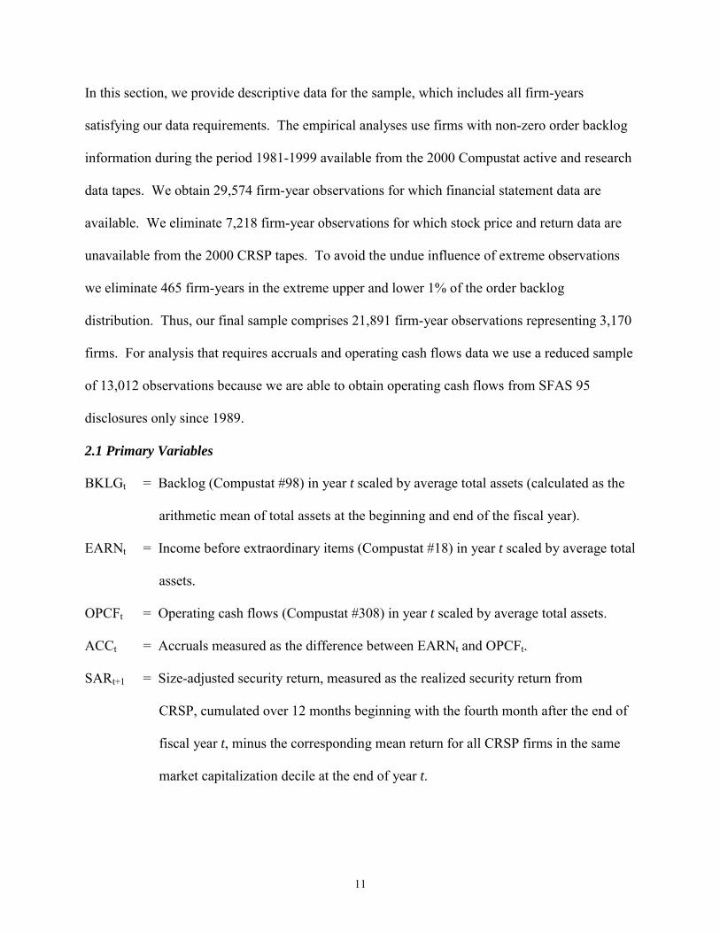
In this section, we provide descriptive data for the sample, which includes all firm-years

satisfying our data requirements. The empirical analyses use firms with non-zero order backlog

information during the period 1981-1999 available from the 2000 Compustat active and research

data tapes. We obtain 29,574 firm-year observations for which financial statement data are

available. We eliminate 7,218 firm-year observations for which stock price and return data are

unavailable from the 2000 CRSP tapes. To avoid the undue influence of extreme observations

we eliminate 465 firm-years in the extreme upper and lower 1% of the order backlog

distribution. Thus, our final sample comprises 21,891 firm-year observations representing 3,170

firms. For analysis that requires accruals and operating cash flows data we use a reduced sample

of 13,012 observations because we are able to obtain operating cash flows from SFAS 95

disclosures only since 1989.

2.1 Primary Variables

BKLGt = Backlog (Compustat #98) in year t scaled by average total assets (calculated as the

arithmetic mean of total assets at the beginning and end of the fiscal year).

EARNt = Income before extraordinary items (Compustat #18) in year t scaled by average total

assets.

OPCFt = Operating cash flows (Compustat #308) in year t scaled by average total assets.

ACCt = Accruals measured as the difference between EARNt and OPCFt.

SARt+1 = Size-adjusted security return, measured as the realized security return from

CRSP, cumulated over 12 months beginning with the fourth month after the end of

fiscal year t, minus the corresponding mean return for all CRSP firms in the same

market capitalization decile at the end of year t.

12

Following Sloan (1996), we control for Fama and French (1992) factors (size, book-to-

market and beta) and prior-year earnings scaled by share price (Basu, 1977) to rule out alternate

explanations for any anomalous security returns. In particular, we consider four variables:

SIZEt = the natural log of the market-value of common equity (MVE), measured at four

months after fiscal year-end.

LnBM t = the natural log of the ratio of book value of common equity to the market

value of common equity (BM), measured at four months after fiscal year-end.3

BETA t = the CAPM beta estimated from a regression of raw monthly returns on the CRSP

value-weighted monthly return index over a period of 60-months ending

four months after each firm�s fiscal year-end.4

EPt = earnings per share divided by stock price measured at four months after fiscal year-end.

Descriptive data related to these variables are reported in Panels A and B of Table 1.

Backlog for the average (median) firm is 46% (30%) of average total assets. The earnings for an

average (median) firm are 0% (4%) of average total assets. Backlog is a large proportion of

average total assets relative to earnings (as a proportion of total assets) because backlog

represents future sales. On average, accruals are negative, consistent with depreciation being a

dominant accrual for these firms. Panel C presents data on the potential relation between order

backlog deflated by assets (i.e., BKLG) and other firm characteristics such as backlog deflated

by sales, earnings, cash flows, and accruals, Fama and French (1992) risk factors, and other

variables shown to predict future returns. In particular, we form ten portfolios sorted on order

backlog (deflated by assets) and report the means of various characteristics of firms in these

portfolios. We find that backlog deflated by sales closely follows the distribution of backlog

deflated by assets. Other than that, there are no clear patterns between BKLG and the reported

13

firm characteristics. Thus, the descriptive evidence presented in panel C indicates prima facie

that BKLG is not strongly related to other well documented anomalies, although we investigate

this issue in greater depth later in the paper. The correlations reported in panel D confirm that

indication. In Panel E we provide the industry composition for our sample firms. Note that a

substantial number of observations (over 70% of the sample) come from two industries - durable

manufacturing and computers (discussed further below).

----Table 1 about here --- 3. Empirical Analyses

We present the empirical tests in several stages. In sections 3.1 and 3.2 we estimate the

historical relation between backlog and future earnings, and the relation between backlog and

future earnings implicit in security prices. A comparison of these historical and market-inferred

weights using the Mishkin (1983) test indicates whether investors correctly appreciate the

importance of order backlog for future earnings. In section 3.3 we investigate whether abnormal

returns can be earned by exploiting investors� misweighting of the contribution of order backlog

to future earnings. In section 4, we examine whether equity analysts use backlog information in

an efficient manner while forecasting future earnings. Finally, we also assess whether market

inefficiencies with respect to backlog are present after controlling for information in analysts�

forecasts.

3.1. Mishkin Test Our initial empirical tests employ the Mishkin (1983) framework to test whether the stock

market is efficient in impounding the information contained in backlog for future earnings. This

framework, introduced by Sloan (1996) to the accounting literature, has since been used by a

number of studies that test for market efficiency. We infer mispricing if the valuation coefficient

14

attributed to backlog by market participants is different from the weight in the association

between backlog and future earnings.

Similar to prior research, we jointly estimate a forecasting specification for the leading

indicator and the rational expectations pricing specification. We extend the earnings forecasting

equation in Sloan (1996) to incorporate the implications of order backlog for future earnings as

follows (firm subscripts suppressed):

EARNt+1 = ω0 + ω1 EARNt + ω2 BKLGt + εt+1 (1)

The coefficient ω1 represents earnings persistence while ω2 captures the incremental contribution

of current order backlog for future earnings. Note that backlog is denominated in sales dollars.

Hence, ω2 incorporates the joint effect of i) the probability of conversion of order backlog into

future sales; and ii) the accounting rate of return (margins) on such converted sales. For the

purposes of our analyses, we assume ω2 is a cross-sectional constant.5

Next, we assume that the market reacts to unexpected earnings conditioned on last year�s

earnings and order backlog. That is:

SARt+1 = β0 + β1 UEARNt+1 + νt+1 (2)

where UEARNt+1, the unexpected earnings variable, is decomposed into realized earnings,

EARNt+1, and expected earnings, E(EARNt+1) with E(.) as the expectation operator:

UEARNt+1 = EARNt+1 � E (EARNt+1) (3)

We substitute the linear prediction of EARNt+1 in equation (1) for expected earnings E(EARNt+1)

embedded in equation (3), and rewrite equation (2) as:

SAR t+1 = β0 + β1 (EARNt+1 � ω0* - ω1* EARNt - ω2* BKLGt) + νt+1 (4)

We refer to equation (4) as the returns equation. Market efficiency with respect to

backlog imposes the constraint that ω2* from the returns equation (4) is the same as ω2 from

15

forecasting equation (1). This nonlinear constraint requires that the stock market rationally

anticipate the implications of current order backlog for future earnings. If ω2 > ω2*, the market

assesses a lower contribution of backlog to future earnings than that warranted by the underlying

cross-sectional association of backlog and future earnings. On the other hand, if ω2 < ω2*, the

market assesses a higher contribution of backlog to future earnings than is warranted.

The two equations in the system are estimated using iterative weighted non-linear least

squares (Mishkin 1983). Market efficiency is tested using a likelihood ratio statistic which is

distributed asymptotically chi-square (q):

2*n* ln (SSRc / SSRu) (5)

where

q = the number of constraints imposed by market efficiency, n = the number of observations in each equation, SSRc = the sum of squared residuals from the constrained weighted system, and SSRu = the sum of squared residuals from the unconstrained weighted system.

3.2. Mishkin Test Results Our initial analyses compare the historical relation between backlog and realized earnings

to the relation between backlog and earnings expectations embedded in security prices. Table 2

reports the historical relation between realized earnings, EARNt+1, and order backlog, BKLGt,

and the stock market�s implicit weighting of order backlog. The coefficient on earnings in the

forecasting equation, ω1 is 0.581 and is statistically different from zero. This coefficient

represents the persistence of the accounting rate of return on assets and is less than unity,

implying thereby that accounting rates of return are mean-reverting (Beaver, 1970; Freeman,

Ohlson, and Penman, 1982). The coefficient on earnings in the returns equation (4), ω1* is 0.536,

but is only weakly different from its counterpart in the forecasting equation (1): the likelihood

16

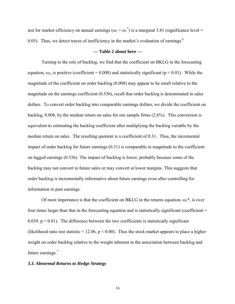
test for market efficiency on annual earnings (ω1 = ω1*) is a marginal 3.81 (significance level =

0.05). Thus, we detect traces of inefficiency in the market�s evaluation of earnings.6

--- Table 2 about here ---

Turning to the role of backlog, we find that the coefficient on BKLG in the forecasting

equation, ω2, is positive (coefficient = 0.008) and statistically significant (p < 0.01). While the

magnitude of the coefficient on order backlog (0.008) may appear to be small relative to the

magnitude on the earnings coefficient (0.536), recall that order backlog is denominated in sales

dollars. To convert order backlog into comparable earnings dollars, we divide the coefficient on

backlog, 0.008, by the median return on sales for our sample firms (2.6%). This conversion is

equivalent to estimating the backlog coefficient after multiplying the backlog variable by the

median return on sales. The resulting quotient is a coefficient of 0.31. Thus, the incremental

impact of order backlog for future earnings (0.31) is comparable in magnitude to the coefficient

on lagged earnings (0.536). The impact of backlog is lower, probably because some of the

backlog may not convert to future sales or may convert at lower margins. This suggests that

order backlog is incrementally informative about future earnings even after controlling for

information in past earnings.

Of most importance is that the coefficient on BKLG in the returns equation, ω2*, is over

four times larger than that in the forecasting equation and is statistically significant (coefficient =

0.039, p < 0.01). The difference between the two coefficients is statistically significant

(likelihood ratio test statistic = 12.06, p < 0.00). Thus the stock market appears to place a higher

weight on order backlog relative to the weight inherent in the association between backlog and

future earnings.7

3.3. Abnormal Returns to Hedge Strategy

17

The preceding section uses the Mishkin test to demonstrate that the stock market overprices

backlog information. However, the Mishkin test is not direct evidence of market inefficiency

for at least two reasons (see Beaver and McNichols, 2001; Wahlen, 2001). First, model

misspecification or the assumptions implicit in the Mishkin procedure (such as linearity of the

model specification, and efficient stock market pricing of omitted variables) may cause an

illusion of market inefficiency (see Kraft, Leone, and Wasley, 2001). Second, because the

coefficients are estimated from a set of contemporaneous observations, the procedure suffers

from a �look-ahead� bias. Investors do not know the implications (i.e., the weight) of backlog

for future earnings until later in the sample period. Hence, we turn to an additional test, the

ability of portfolios formed on the cross-sectional distribution of backlog to predict future

abnormal returns.

The strategy we implement relies on the construction of zero-investment portfolios (Fama

and MacBeth, 1973). Portfolios are formed as follows: First, for each year from 1981 to 1999,

we calculate the scaled decile rank for BKLGt for each firm. In particular, we rank the values of

BKLGt into deciles (0,9) each year and divide the decile number by nine so that each observation

related to BKLGt takes a value ranging between zero and one. We estimate the following cross-

sectional OLS regression for each of the 19 years in the sample:

SAR t+1 = γ0 + γ1BKLGtdec + φt+1 (6)

The basic idea behind the Fama and MacBeth (1973) regressions is to project the size-

adjusted returns on the intercept and the BKLGtdec variable for each cross section and then

aggregate the estimates over the 19 years. Tests of statistical significance of γ1 are based on the

standard error calculated from the distribution of the individual yearly coefficients. This test

18

overcomes bias due to cross-sectional correlation in error terms but assumes independence in

error terms across time (Bernard, 1987).

Coefficient γ1 represents the size-adjusted abnormal return to a zero-investment portfolio

optimally formed to exploit the information in the backlog variable. This is because the weights

assigned to each firm in the BKLGdec variable, represented by the rows of the matrix (X'X)-1X',

where X = [1, BKLGdect], sum to zero. Because the portfolio weights are determined without

foreknowledge of future abnormal returns, we are investigating executable trading strategies.

Our strategy involves taking positions in firms that have reported results within 4 months of the

fiscal-year end to allow for the determination of portfolio weights from (X'X)-1X' used to

ascertain the investment positions. Thus, firms receiving negative weights are sold short and

firms with positive weights are bought. The long and short positions are closed after one year.

The abnormal returns, represented by coefficient γ 1, are comparable to abnormal returns to a

zero-investment portfolio with long (short) positions in firms within the lowest (highest) deciles

of backlog (see Bernard and Thomas, 1990).

Results from the Fama-MacBeth regressions reported in Table 3 generally confirm the

findings from the Mishkin test. There is a negative relation (coefficient = -0.058) between

BKLG and future returns that is statistically significant (t-statistic of 2.38, p < 0.05). The

negative sign on the coefficient on BKLG is consistent with the difference in historical and

security-market weightings of the contribution of current backlog to future earnings documented

using the Mishkin framework. Because the market overestimates the future earnings

implications of backlog we should observe negative abnormal returns for portfolios ranked on

backlog. Thus, the abnormal return of 5.8% to a trading strategy based on order backlog is both

statistically and economically significant.

19

--- Table 3 about here ---

3.4. Robustness Checks and Sensitivity Analyses

3.4.1. Controlling for Fama-French Factors and the Basu (1977) Anomaly

Prior research has shown that future abnormal returns are associated with other variables, such as

firm size (SIZE), book-to-market ratio (BM), and systematic risk (BETA). Fama and French

(1992) conjecture that these variables reflect unknown risk factors and, hence, are associated

with future expected returns. Although panels C and D of Table 1 report the absence of strong

relations between BKLG and the Fama-French factors, to be consistent with standard practice in

recent asset-pricing literature, we investigate whether abnormal returns related to backlog are

independent of returns observed in connection with the Fama-French factors. We also include

the earnings-to-price ratio (EP) to control for the earnings-price anomaly documented by Basu

(1977).

To assess whether the backlog anomaly generates incremental returns to the Fama-French

factors and the Basu anomaly, we estimate the following regression:

SAR t+1 = γ0 + γ1 BKLGdect + γ2 SIZEdec

t + γ3 BETAdect + γ4 LnBMdec

t + γ5 EPdect + ϕt+1 (7)

where SIZEdect, BETAdec

t, and LnBMdect relate to scaled decile ranks (ranging from 0 to 1) for

the three Fama-French factors. EPdect refers to scaled decile ranks of the earnings-price ratio. In

the regression specification (7), coefficient γ1 represents the incremental size-adjusted abnormal

return to a zero-investment portfolio in the backlog variable.

Results reported in panel B of Table 3 indicate that incremental abnormal returns related

to BKLG persist after controlling for potentially confounding variables. However, controlling

for Fama-French factors and the Basu anomaly reduces the incremental return to the BKLG

based hedge portfolio to 4.8% from 5.8% in panel A with no controls. Turning to the control

20

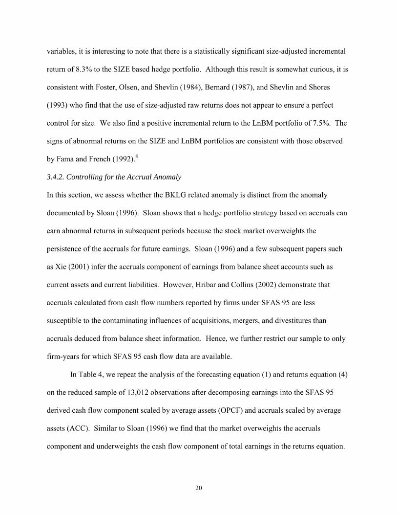
variables, it is interesting to note that there is a statistically significant size-adjusted incremental

return of 8.3% to the SIZE based hedge portfolio. Although this result is somewhat curious, it is

consistent with Foster, Olsen, and Shevlin (1984), Bernard (1987), and Shevlin and Shores

(1993) who find that the use of size-adjusted raw returns does not appear to ensure a perfect

control for size. We also find a positive incremental return to the LnBM portfolio of 7.5%. The

signs of abnormal returns on the SIZE and LnBM portfolios are consistent with those observed

by Fama and French (1992).8

3.4.2. Controlling for the Accrual Anomaly

In this section, we assess whether the BKLG related anomaly is distinct from the anomaly

documented by Sloan (1996). Sloan shows that a hedge portfolio strategy based on accruals can

earn abnormal returns in subsequent periods because the stock market overweights the

persistence of the accruals for future earnings. Sloan (1996) and a few subsequent papers such

as Xie (2001) infer the accruals component of earnings from balance sheet accounts such as

current assets and current liabilities. However, Hribar and Collins (2002) demonstrate that

accruals calculated from cash flow numbers reported by firms under SFAS 95 are less

susceptible to the contaminating influences of acquisitions, mergers, and divestitures than

accruals deduced from balance sheet information. Hence, we further restrict our sample to only

firm-years for which SFAS 95 cash flow data are available.

In Table 4, we repeat the analysis of the forecasting equation (1) and returns equation (4)

on the reduced sample of 13,012 observations after decomposing earnings into the SFAS 95

derived cash flow component scaled by average assets (OPCF) and accruals scaled by average

assets (ACC). Similar to Sloan (1996) we find that the market overweights the accruals

component and underweights the cash flow component of total earnings in the returns equation.

21

Specifically, the coefficient on operating cash flows in the forecasting equation, ω1a, is 0.726,

whereas the coefficient on operating cash flows in the returns equation, ω1a*, is 0.586 and the

difference is significant at conventional levels (likelihood ratio statistic = 11.84, p < 0.01). The

coefficient on accruals in the forecasting equation, ω1b, is 0.390 whereas its counterpart in the

returns equation, ω1b*, is 0.557 (likelihood ratio statistic = 15.31, p < 0.01). Most important,

however, the market continues to overweight BKLG in the returns equation (ω2* is 0.052)

compared to the weight on BKLG in the forecasting equation (ω2 is 0.005) and the difference is

statistically significant (likelihood ratio statistic is 13.91, p < 0.00). Thus, the BKLG anomaly is

incremental to the accruals anomaly documented by Sloan (1996).

--- Table 4 about here ---

To ensure that abnormal returns can be earned from the BKLG anomaly incremental to

those from the accrual anomaly, we augment the Fama-Macbeth type equation (7) with an

additional regressor, ACCdect. This variable represents accruals for year t divided by average

assets ranked into deciles (0,9) each year and scaled by nine so that each observation takes a

value ranging between zero and one.

Panel A of Table 5 reports the results of assuming hedge positions on order backlog for

the reduced sample of firm-years with SFAS 95 data. It turns out that the hedge portfolio return

for the reduced sample is higher at 8.1% as compared to the full sample return of 5.8% reported

earlier. Systematic differences between the reduced sample and the full sample could potentially

account for the higher return on the backlog variable in the reduced sample. For example, we

find that firms in the reduced sample are systematically larger on average (t-statistic to assess

difference in means is 11.43) and have smaller CAPM betas (t-statistic for difference of means is

7.54).

22

--- Table 5 about here ---

Panel B of Table 5 shows that the introduction of Fama-French factors and both the Sloan

and the Basu anomaly do not affect abnormal returns from the BKLG anomaly.9 A zero-

investment strategy on BKLG variable earns incremental abnormal returns of 7.7%.10 In contrast,

Sloan�s accrual strategy appears to earn an incremental abnormal return of 16.6%. Notice that

the negative coefficient on the accruals variable is consistent with the market overreacting to

accruals. Thus, the BKLG strategy earns as much as 46% of the returns from Sloan�s anomaly.11

3.4.3. Additional Sensitivity Analyses

In this section we conduct several additional tests to further assess the robustness of our results.

We begin by considering the sensitivity of our analysis to the assumption of a single-lag relation

of backlog for future earnings. It is quite likely that backlog follows a more complicated process

and investors may also use a more sophisticated expectations model; as a result, our estimates of

the weights implicit on backlog in the estimation equation (ω2) and valuation weight placed by

investors on backlog (ω2*) may be biased. However, following Mishkin (1983) and Abel and

Mishkin (1983), Sloan (1996) argues that the tests of cross-system non-linear constraints remain

valid tests of market efficiency regardless of whether the forecasting equation has omitted

variables (such as a second-lag backlog term). Abel and Mishkin (1983) and Mishkin (1983)

also point out that if the model generating the dependent variables (earnings at t+1 in our setting)

is incorrectly specified, then the standard errors-in-variables problem arises, meaning estimates

of the valuation equation weights, ω1* and ω2*, will be inconsistent, and the test will have lower

power. Rejection of the null hypothesis of efficiency with a test of known low power would be

an even stronger case against efficiency. Thus, our inferences about the degree to which

23

information in prior backlogs is incorporated into the earnings expectations process are likely to

be robust to the actual time series process and the form of investor expectations.

Furthermore, as Soffer and Lys (1999) point out in their appendix 3, ω2 can be viewed as

a weighted average of the extent to which future earnings are related to prior backlog lags that

are correlated with the first lag. Similarly, ω2* can be viewed as a weighted average of the

extent to which investors have incorporated information from prior backlog lags that are

correlated with the first lag. Thus we capture, in a single measure, the degree to which all

information correlated with the first lag is incorporated into earnings expectations. Considering

that the correlation between first-lag of backlog and the second-lag is very high (ρ = 0.87) in our

sample, we argue that modeling the first lag alone is reasonable for the purpose of assessing

deviation from market efficiency with respect to the information in order backlog.

Notwithstanding the above arguments, we incorporate a second-lag of backlog into the

earnings estimation equation (1) and (4) and test whether the weights placed by the market on

both lags of backlog in equation (4�) below are consistent with weights in the forecasting

equation (1�).

EARNt+1 = ω0 + ω1 EARNt + ω2 BKLGt + ω3 BKLGt-1 + εt+1 (1�)

SAR t+1 = β0 + β1 (EARNt+1 � ω0* - ω1* EARNt - ω2* BKLGt - ω3* BKLGt-1) + νt+1 (4�)

The joint test of efficiency (i.e., ω2 = ω2*; ω3 = ω3*) is rejected at conventional levels. More

important, the results (unreported) indicate that the market prices BKLGt-1 (not BKLGt) in an

inefficient manner. This result is probably not surprising given the high correlation between

BKLGt and BKLGt-1. An implication of this finding is that abnormal returns can be earned on

BKLG positions for a period longer than one year. Indeed, we do observe (results not reported)

the presence of abnormal returns on BKLGdec portfolios for three years into the future, after

24

which the abnormal returns are no longer statistically significant. The disappearance of abnormal

returns after three years also suggests that an omitted risk factor cannot explain our findings.

Recall that the coefficient mapping BKLG to future earnings (EARN), is constrained to

be a cross-sectional constant in equation (1). To assess whether our results are sensitive to that

assumption, we perform two sensitivity checks. First, we estimate the earnings forecasting

equation (1) and the returns equation (4) separately for two main industry groups in our sample �

durable manufacturers and computers. Separate estimation by industry does not constrain the

predictive ability of order backlog for future earnings to be a cross-sectional constant. In

unreported results, we find that the market overweights backlog relative to its contribution to

future earnings in both industries. Second, we estimate future earnings from BKLG and

investigate whether investors misprice such earnings. In particular, we construct a new variable,

BKLG-GM, defined as the product of BKLG and the gross margin percentage (1- cost of goods

sold/sales) and substitute that variable in place of BKLG in equations (1) and (4).12 The

unreported results of the Mishkin test indicate that the market continues to overweight the

relation between BKLG-GM and future earnings. In particular, coefficient ω2 on BKLG-GM in

equation (1) is 0.020 whereas investors price BKLG-GM at 0.118 (coefficient ω2*) and the

difference is statistically significant (likelihood ratio statistic = 9.80, p < 0.00). Taken together,

our reported results are not due to the assumption of homogeneity on the conversion of backlog

across industries.

Finally, we assess whether our results are sensitive to the deflator used to scale order

backlog, by using sales as a deflator instead of average total assets in equations (1)

and (4). The untabulated results from this procedure are similar to those reported in the paper.13

4. Do Analysts Appreciate the Implications of Backlog for Future Earnings?

25

In this section we explore whether sophisticated market intermediaries, such as equity analysts,

understand the implications of order backlog for future earnings when they generate earnings

forecasts. Lev and Thiagarajan (1993) identify order backlog as one of the fundamental

variables that analysts appear to use beyond GAAP information. Francis, Schipper, and Vincent

(2003) isolate order backlog as a leading indicator in the home-building industry based on their

assessment of industry reports, analyst reports and popular press articles. Research by Barth,

Kasznik, and McNichols (2001) suggests that financial analysts likely aid investors� assessment

of non-GAAP information. Hence, arguments made in the prior literature support the conjecture

that analysts incorporate backlog data into their earnings forecasts. On the other hand, other

research (Klein, 1990; Abarbanell, 1991; Mendenhall, 1991; Abarbanell and Bernard, 1993; Ali,

Klein, and Rosenfeld, 1992) finds that analysts do not fully utilize available information

efficiently while setting earnings forecasts. Thus, whether analysts incorporate order backlog in

a manner consistent with the cross-sectional association of backlog to future earnings is an open

question.

To address this question we regress future earnings on scaled decile ranks of backlog and

compare the coefficient on backlog ranks with the coefficient from a regression of analyst

forecast of future earnings on these backlog ranks. We estimate the following specifications:

EPSt+1 = δ0 + δ1 EPSt + δ2 BKLGdect + µt+1 (8)

FEPSt+1 = λ0 + λ1 EPSt + λ2 BKLGdect + ηt+1 (9)

FERRt+1 = (δ0- λ0) + (δ1- λ1) EPSt + (δ2- λ2) BKLGdect + (µt+1 - ηt+1) (10)

where FERR is the forecast error computed as the difference between EPSt+1 and FEPSt+1, EPSt+1

is earnings per share for the fiscal year t+1 scaled by stock price at the end of fiscal year t, and

FEPSt+1 if the forecasted year t+1 earnings per share made four months after the end of year t

26

(deflated by stock price at four months after the end of year t).14 We use backlog ranks as

opposed to backlog scaled by average assets to avoid concerns about mismatch in the scaler used

for EPS and FEPS variables.15

Coefficients δ1 and δ2 represent the information content of past earnings and backlog in

forecasting future earnings. Coefficients λ1 and λ2 represent weights that analysts attach to past

earnings and backlog, respectively. The coefficients on the forecast error specification indicate

the difference between the implied weight on backlog (past earnings) for future earnings and the

analysts� weights on backlog (past earnings) in forecasting future earnings. If analysts fail to

adequately incorporate the implications of backlog for future earnings, the coefficient on BKLG

(i.e., δ2-λ2) in equation (10) will be different from zero.

To conduct the analysis, we obtain analysts� consensus earnings forecasts from I/B/E/S.

Because the definition of accounting earnings in I/B/E/S is often different from that in the

Compustat tapes (Abarbanell and Lehavy, 2000) we obtain realized earnings from I/B/E/S for the

purpose of this analysis. This procedure also ensures comparability between analysts� forecasts and

realized earnings. From the I/B/E/S tapes we are able to obtain analyst forecasts for 11,259

observations for the period 1981-1999. Descriptive statistics relating to forecast earnings and

corresponding reported earnings are presented in panel A of Table 1.

Table 6 reports the results of estimating equations (8)�(10). We report mean estimates

from annual cross-sectional regressions. Test-statistics and significance levels of the mean

estimates are again determined using inter-temporal t-tests (see Bernard, 1987). The estimated

coefficient on past earnings per share in earnings forecasting equation (8), i.e., δ1, is 0.488 (see

Panel A of Table 6). The earnings persistence based on I/B/E/S earnings variables is comparable

to the earnings persistence of 0.58 obtained using earnings scaled by average total assets (see

27

Table 2). However, the coefficient on past earnings per share in the analysts� forecasting

equation (9), i.e., λ1, is just 0.221 (see Panel B of Table 6). As is evident from Panel C of Table

7, the difference (δ1 - λ1) is statistically significant at the 1% level (coefficient = 0.267, t = 2.99).

This result is consistent with prior research (Ahmed et al., 2002) that finds analysts under-

estimate the time-series persistence of earnings.

--- Table 6 about here ---

As with the results obtained earlier we find that order backlog information has

implications for future earnings (δ1 = 0.016, t = 3.29). Consistent with the hypothesis that

analysts� forecasts incorporate information in order backlog in addition to information in past

realized earnings, we find that the coefficient on order backlog, λ2, in equation (9) is statistically

positive (coefficient = 0.017, t = 5.07). Furthermore, there is no statistical difference between

the two coefficients. That is, the coefficient (δ2 - λ2) reported in Panel C is not significantly

different from zero. Thus, the results indicate that analysts use backlog information to forecast

future earnings in a manner consistent with the association between backlog and future earnings.

If analysts correctly incorporate the implication of backlog for future earnings, then why

do we observe abnormal returns on order backlog positions? One possibility is that the stock

market overweights backlog information only in firms with low analyst coverage.16 Walther

(1997) and Elgers, Lo, and Pfeiffer (2001) find that the market does not correctly impound the

information in analyst forecasts when firms are covered by fewer analysts. However, we find (in

untabulated analyses) that the backlog anomaly is robust in firms with high analyst coverage

(proxied by firms where number of analysts covering a firm is above the median) as well.

28

Another possibility is that investors fixate on order backlog even though analyst

forecasts efficiently impound its future-earnings effects. To assess this possibility, we estimate

the following regressions:

EPSt+1 = α0 + α1 EPSt + α2 FEPSt+1 + α3 BKLGdect + φt+1 (11)

SARt+1 = ζ0 + ζ1 (EPSt+1 - α0 - α1

* EPSit - α2

* FEPSt+1 - α3* BKLGdec

t) + πt+1 (12)

Equations (11) and (12) are estimated using the Mishkin procedure described earlier. In

equation (11), the coefficient α3 is predicted to be statistically insignificant because the median

analyst forecast, FEPSt+1, already incorporates the forecast of future earnings from backlog. If

investors correctly appreciate the role of order backlog as it relates to future earnings, we would

expect to observe α3* in equation (12) to be insignificant as well.

Table 7 reports the results of estimating equations (11) and (12). Coefficient α3 is

statistically insignificant, as expected. Thus, backlog is not incrementally useful for forecasting

future earnings over analyst forecasts because analysts already efficiently incorporate backlog

information in their forecasts. However, coefficient α3* in the returns equation (12) is positive

and statistically significant consistent with market mispricing information in order backlog. The

likelihood ratio test to assess the equality of coefficient α3 and α3* can be comfortably rejected at

conventional levels of significance (12.15, p < 0.00). Thus, it appears that the stock market

fixates on order backlog although equity analysts appear to correctly use backlog information in

forecasting future earnings. The simultaneous existence of analysts� efficiency with respect to

public information and the stock market�s inefficiency with respect to the same public

information is not without precedent. Doukas, Kim, and Pantzalis (2002) find that analysts�

forecasts and revisions do not exhibit the value-glamour anomaly documented for the stock

market as a whole by Lakonishok, Shleifer, and Vishny (1994) and La Porta et al. (1997).

29

--- Table 7 about here ---

A couple of other findings from equations (11) and (12) are worthy of comment.

Consistent with Sloan (1996), we find that the market does not misweight earnings persistence as

the likelihood ratio test cannot reject the equality of earnings coefficient α1 and α1* at

conventional levels of significance (likelihood ratio statistic is 0.00, p = 0.96). However, the

stock market appears to misweight the role of analyst forecasts in predicting future realized

earnings. Coefficient α 2 on analyst forecasts in the earnings-equation (11) is 0.764, whereas

coefficient α2* on analyst forecasts in the returns-equation (12) is higher at 1.310 and the

difference is statistically significant (likelihood ratio test = 8.64, p < 0.00). Thus, stock market

participants appear to overweight the role of analyst forecasts in predicting future earnings. Prior

literature (e.g., Walther, 1997; Elgers, Lo, and Pfeiffer, 2001) also provides evidence consistent

with investors failing to correctly impound analysts� forecasts, although these papers find that

investors underweight analyst forecasts.

5. Conclusions Previous research has interpreted the value-relevance of leading indicators in an efficient market

context as indicative of future earnings prospects of firms. However, the content and

presentation of the disclosures related to leading indicators is not standardized by GAAP. A

recent FASB report finds that extant disclosures of such indicators are patchy and inconsistent.

Hence, we explore the alternate hypothesis that the stock market possibly misprices these leading

indicators. We examine one aspect of such mispricing by investigating whether security prices

rationally anticipate the role of current backlog for future earnings.

We find that market expectations are inconsistent with the traditional efficient markets

view that stock prices fully reflect publicly available information about the association between

30

current leading indicators and future earnings. In particular, the market behaves as though the

contribution of backlog to future earnings is larger than that warranted by the earnings prediction

model. This anomaly can be exploited to earn abnormal hedge strategy returns, and such returns

are incremental to returns expected on account of Fama-French factors, Basu�s (1977) earnings-

price anomaly and Sloan�s (1996) accrual anomaly.

We probe deeper to evaluate whether analysts correctly appreciate the role of backlog in

predicting future earnings. We find that analysts incorporate backlog information into their

equity forecasts in a manner consistent with the relation between backlog and future earnings.

However, investors appear to value backlog incremental to analyst forecasts that already include

the implications of backlog for future earnings. Thus, the backlog anomaly persists in spite of

analyst forecast efficiency possibly because the stock market fixates on order backlog

information.

Our findings have several implications. The assumption of market efficiency in prior

studies on the value-relevance of non-GAAP indicators may be open to question. Because

investors have trouble appreciating the future-earnings implications of backlog for a set of

relatively mature industries such as durable manufacturers and computers, it is not a stretch to

conjecture that investors likely over-value leading indicators in technology-intensive and early-

stage businesses focused on wireless operations and the Internet. It is also worth noting that

stock analysts in these industries often rely on ratios based on such indicators in their reports

(e.g., price-to-POPS ratio in the wireless industry and price-to-eyeballs ratio in the Internet

sector). Moreover, regulators cite evidence on the value-relevance of non-GAAP leading

indicators (see FASB, 2001; SEC, 2001) in policy papers that recommend enhanced disclosure

of forward-looking information. Given the documented over-weighting of backlog information,

31

perhaps standard-setting bodies could consider asking firms to report explicit data about how

leading indicators might map into future earnings. An example of such disclosure might be the

expected margins on order backlog. We hasten to add that policy recommendations based on

empirical archival research are hazardous on account of difficulties associated with extrapolation

of results from one study and the complex balancing of social costs and benefits of increased

disclosure.

Acknowledgments

We thank an anonymous referee, Bruce Behn, Bokhyeon Baik, Jennifer Francis, John Hand, Pat

Hopkins, Ed Maydew, Michael Mikhail, Steve Penman (editor), Madhav Rajan, Richard Willis

and workshop participants at Duke University, Columbia University, the 2001 University of

Texas-Dallas symposium, University of California at Irvine, and the 2002 BMAS conference at

the University of Texas-Austin and the 2002 AAA meetings at San Antonio for helpful

comments. We appreciate financial support from the Accounting Development Fund at the

University of Washington, Fuqua School of Business, Duke University and the Graduate School

of Business, Stanford University.

32

Notes 1 Recent research (Collins, Maydew and Weiss, 1997; Francis and Schipper, 1999) appears to

support this claim. However, others question whether financial measures have lost relevance

over time (Brown, Lo, and Lys, 1999; Landsman and Maydew, 2002; and Core, Guay, and

Buskirk, 2003).

2 One plausible reason for such an omission is that many of the technology-intensive industries

examined have long gestation lags from product conception to profitability and are hence likely

to report negative earnings in the short-run. Moreover, equity analysts usually do not forecast

future earnings beyond three years and the near-term forecasts of future earnings in technology

intensive industries may still be negative.

3 Whenever the equity book value is negative we replace the BM variable with the lowest

number from the distribution of natural log of the book to market ratio.

4 In estimating the beta we require that monthly return data be available for a minimum of 10

months to enable efficient estimates.

5 We examine the implications of this assumption in sensitivity analyses (section 3.4.3).

6 While this result may appear inconsistent with Sloan�s (1996) finding of market efficiency with

respect to information in past earnings, our unreported results using observations from two sub-

samples used later in the paper (sample of SFAS 95 accrual data in section 3.4.2 and analyst

forecast sample in section 4) indicate no market inefficiency with respect to the time-series

properties of earnings. Furthermore, as reported below, we do not find abnormal returns to the

EP anomaly, thereby suggesting market efficiency with respect to past earnings.

7 In untabulated results using decile rankings of BKLG and EARN instead of actual values, we

continue to find that the stock market does not appear to rationally anticipate the lower

33

contribution of backlog for future earnings. That is, ω2* > ω2 and the likelihood ratio statistic to

test the equality of ω2* and ω2 is 11.63 (p < 0.01).

8 We do not observe any significant time-based clustering of significant coefficients. Out of 10

significant coefficients in Table 3 related to BKLG, four coefficients (1983, 1985, 1987 and

1989) are significant before 1990 and the remaining coefficients (1991, 1993, 1994, 1995, 1998

and 1999) are significant after 1990. In Table 5 (to follow), the six significant coefficients are in

1989, 1990, 1992, 1994, 1995 and 1999.

9 We also control for industry differences by including industry dummies and our inferences are

unaltered.

10 Transactions costs are unlikely to be a major hurdle in exploiting the BKLG anomaly. If a

trader wants to exploit the accrual and the BKLG anomaly, the incremental costs of exploiting

the BKLG anomaly are likely to be trivial. The positions that the trader needs to take to exploit

the accrual anomaly can be netted against those that he needs to take to exploit the BKLG

anomaly, thereby requiring a single trade to achieve the optimal weights in all portfolios.

11 The magnitude of the abnormal return on Sloan�s strategy is larger than the 10.4% that he

documents. This possibly occurs for four reasons. First, Hribar and Collins (2002) show that

accruals backed out of balance sheet accounts such as current assets and current liabilities, as

computed by Sloan, instead of SFAS 95 data tend to understate the extent of abnormal returns

that can be earned from Sloan�s anomaly. Second, Sloan�s sample comes from the years 1962-

1991, whereas our sample in these tests covers the years 1989-1999. Thus, time-period specific

issues might have also influenced our findings. Third, Sloan focuses only on the lowest and

highest deciles, whereas we focus on Fama and Macbeth (1973) type trading strategy that assigns

weights to firms in every decile. In Sloan�s study if one were to focus on the extreme quintiles

34

as opposed to extreme deciles one could earn abnormal returns of 16.7%. Finally, our reduced

sample is an intersection of firms with backlog data and SFAS 95 data. Hence, the abnormal

returns may be different for firms with non-zero backlog.

12 We use gross margins in lieu of return on sales because a significant number of observations

have negative earnings.

13 Another potential sensitivity analysis is to examine the returns to a backlog strategy around

subsequent earnings announcements, which is particularly relevant when the release of tradable

information such as accruals (about predictable earnings changes) is assumed to be concentrated

in announcement periods. However, this assumption is unlikely to hold in our context. This is

because information about the extent of conversion of backlog into future sales, and hence,

earnings, may not necessarily be revealed around earnings announcements given that (i) retailers

provide periodic same store sales data, (ii) automobile manufacturers provide monthly vehicle

sales information, and (iii) airline manufactures (e.g., Boeing) issue press releases about aircraft

deliveries. Hence, information about the contribution of backlog for future earnings is likely to

be incorporated in stock price at various times throughout the year, not just around earnings

announcements.

14 Consistent with a long tradition in analyst forecast research (e.g., Ali, Klein, and Rosenfeld,

1992 and Abarbanell and Bernard, 1993), we scale the median analyst forecast by market price

and not by average total assets (as in the previous sections of the paper). Scaling by average total

assets, which is obtained from Compustat tapes, requires a conversion of the per-share forecast

numbers to a net income number. This can be accomplished by multiplying the number of

outstanding shares in I/B/E/S by the forecast per share. However, data on the number of shares

outstanding for a significant number of firm-years is missing in the I/B/E/S tapes. In an effort to

35

conserve as many firm-year observations as possible for our empirical analyses, we scale the

analyst forecast by lagged market price per share. To be consistent with the scalar for analyst

forecasts, we scale the earnings variables in equations (8), (9), and (10) by stock price as well.

15 As a sensitivity check, we use actual order backlog scaled by average total assets and find that

our inferences are unaffected.

16 In untabulated results, we find evidence of the stock market continuing to overweight backlog

in firms without analyst coverage, i.e., the sub-sample of firms for which we do not have I/B/E/S

forecasts.

36

References

Abarbanell, J. (1991). �Do Analysts� Forecasts Incorporate Information in Prior Stock Price

Changes?� Journal of Accounting and Economics 14, 147-165.

Abarbanell, J., and V. Bernard. (1993). �Tests of Analysts� Overreaction/Underreaction to

Earnings Information as an Explanation for Anomalous Stock Price Behavior.� Journal

of Finance 47, 1187-1207.

Abarbanell, J., and R. Lehavy. (2000). �Differences in Commercial Database Reported Earnings:

Implications for Inferences Concerning Analyst Forecast Rationality, the Association

between Prices and Earnings, and Firm Reporting Discretion.� Working paper,

University of North Carolina at Chapel Hill and University of Michigan.

Abel, A., and F. Mishkin. (1983). �An Integrated View of Tests of Rationality, Market

Efficiency and the Short Run Neutrality of Monetary Policy.� Journal of Monetary

Economics 11, 3-24.

Ahmed, A.S., K. Nainar, X. Zhang, and J. Zhou. (2002). �Do Analysts' Forecasts Fully Reflect

the Information in Accruals?� Working paper, Syracuse University.

Ali, A., A. Klein, and J. Rosenfeld. (1992). �Analysts� Use of Information about Permanent and

Transitory Earnings Components in Forecasting Annual EPS.� The Accounting Review

67, 183-198.

American Institute of Certified Public Accountants (AICPA). (1994). Improving Business

Reporting – A Customer Focus: Meeting the Information Needs of Investors and

Creditors. New York, NY: AICPA.

37

American Accounting Association (AAA) Financial Accounting Standards Committee. (2002).

�Recommendations on Disclosure of Nonfinancial Performance Measures.� Accounting

Horizons 16, 353-362.

Amir, E., and B. Lev. (1996). �Value-Relevance of Nonfinancial Information: The Wireless

Communications Industry.� Journal of Accounting and Economics 22, 3-30.

Barth, M.E., R. Kasznik, and M. F. McNichols. (2001). �Analyst Coverage and Intangible

Assets.� Journal of Accounting Research 39, 1-34.

Banker, R., G. Potter, and D. Srinivasan. (2000). �An Empirical Investigation of an Incentive

Plan that Includes Nonfinancial Performance Measures.� The Accounting Review 75, 65-

92.

Basu, S. (1977). �The Investment Performance of Common Stocks in Relation to their Price to

Earnings Ratios: A Test of the Efficient Markets Hypothesis.� Journal of Finance 32,

663-662.

Beaver, W.H. (1970). �The Time Series Behavior of Earnings.� Journal of Accounting Research

8, 319-346.

Beaver, W.H., and M.F.McNichols. (2001). �Do Stock Prices of Property Casualty Insurers Fully

Reflect Information about Earnings, Accruals, Cash flows, and Development? Review of

Accounting Studies 6, 197-220.

Behn, B.K. (1996). �Value Implications of Unfilled Order Backlogs.� Advances in Accounting

14, 61-84.

Bernard, V. (1987). �Cross-sectional Dependence and Problems in Inference in Market-based

Accounting Research.� Journal of Accounting Research 25, 1-48.

38

Bernard, V., and J. Thomas. (1990). �Evidence that Stock Prices Do Not Fully Reflect the

Implications of Current Earnings for Future Earnings.� Journal of Accounting and

Economics 13, 305-340.

Brown, S., K. Lo, and T. Lys. (1999). �Use of R2 in Accounting Research: Measuring Changes

in Value Relevance Over the Last Four Decades.� Journal of Accounting and Economics

28, 83-115.

Canadian Institute of Chartered Accountants. (1995). Performance Measures in the New

Economy. Toronto, Canada: CICA.

Chandra U., A. Procassini, and G. Waymire. (1999). �The Use of Trade Association Disclosures

by Investors and Analysts: Evidence from the Semiconductor Industry.� Contemporary

Accounting Research 16, 643-670.

Collins, D.W., E.L. Maydew, and I.S. Weiss. (1997). �Changes in the Value-relevance of

Earnings and Book Values over the Past Forty Years.� Journal of Accounting and

Economics 24, 39-67

Core, J., W Guay, and A.VanBuskirk. (2003). �Market Valuations in the New Economy: An

Investigation of What Has Changed.� Journal of Accounting and Economics 34, 43-67.

D�Avolio, G., E. Gildor and A. Shleifer. (2001). �Technology, Information Production, and

Market Efficiency.� Working paper, Harvard Institute of Economic Research.

Damodaran, A. (2001). The Dark Side of Valuation: Valuing Old Tech, New Tech and New

Economy Companies. New Jersey: Financial Times Prentice Hall.

Demers, E., and B. Lev. (2000). �A Rude Awakening: Internet Value Drivers in 2000,� Review

of Accounting Studies 6, 331-359.

Deng, Z, B. Lev, and F. Narin. (1999). �Science and Technology as Predictors of Stock

39

Performance.� Financial Analysts Journal 55, 20-32.

Doukas, J.A., C. Kim, and C. Pantzalis. (2002). �A Test of the Errors-in-Expectations

Explanation of the Value/Glamour Stock Returns Performance: Evidence from Analysts�

Forecasts.� The Journal of Finance 57, 2143-65.

Eccles, R.G., R. H. Herz, M. Keegan, and D.M.H. Phillips. (2001). The Value Reporting

Revolution:Moving Beyond the Earnings Game. New York: John Wiley & Sons.

Elgers, P.T., M.H. Lo, and R.J. Pfeiffer. (2001). �Delayed Security Price Adjustments to

Financial Analysts' Forecasts of Annual Earnings.� The Accounting Review 76, 613-

632.

Fama, E. and K. French. (1992). �The Cross-section of Expected Returns.� Journal of Finance

47, 427-466.

Fama, E. and J. Macbeth. (1973). �Risk, Return and Equilibrium: Empirical Tests.� Journal of

Political Economy 71, 607-636.

Financial Accounting Standards Board (2001). Business and Financial Reporting: Challenges

from the New Economy, New York: FASB.

Foster, G., C. Olsen, and T. Shevlin. (1984). �Earnings Releases, Anomalies, and the Behavior of

Security Returns.� The Accounting Review 59, 574-604.

Francis J., and K. Schipper. (1999). �Have Financial Statements Lost Their Relevance?�

Journal of Accounting Research 37, 319-352.

Francis, J., K. Schipper, and L. Vincent. (2003). �The Relative and Incremental Information

Content of Alternative (to Earnings) Performance Measures.� Contemporary Accounting

Research 20, 121-164.

Freeman, R., J. Ohlson, and S. Penman. (1982). �Book Rate-of-Return and Prediction of

40

Earnings Changes: An Empirical Investigation.� Journal of Accounting Research 20, 3-

42.

Hribar. P.and D.W. Collins (2002). �Errors in Estimating Accruals: Implications for Empirical

Research.� Journal of Accounting Research 40, 105-134.

Institute of Chartered Accountants in England and Wales. (2000). New Measures for the New

Economy. London: ICAEW.

Ittner, C. and D. Larcker. (1998a). �Are Nonfinancial Measures Leading Indicators of Financial

Performance? An Analysis of Customer Satisfaction.� Journal of Accounting Research

36, 1-36.

Ittner, C. and D. Larcker. (1998b). �Innovations in Performance Measurement: Trends and

Research Implications.� Journal of Management Accounting Research 10, 205-238.

Kaplan, R. and D. Norton. (1996). The Balanced Scorecard. Boston: Harvard Business Press.

Klein, A. (1990). �A Direct Test of the Cognitive Bias Theory of Share Price Reversals.�

Journal of Accounting and Economics 13, 155-166.

Kothari, S.P. (2001). �Capital Markets Research in Accounting.� Journal of Accounting and

Economics 31, 105-231.

Kraft, A., A. Leone, and C. Wasley. (2001). �On the Use of Mishkin�s Rational Expectations

Approach to Testing Efficient-Markets Hypotheses in Accounting Research.� Working

paper, University of Rochester.

Lakonishok, J, A. Shleifer, and R. W. Vishny. (1994). �Contrarian Investments, Extrapolation,

and Risk.� The Journal of Finance, 49, 1541-1578.

Landsman, W. and E.Maydew. (2002). �Has the Information Content of Quarterly Earnings

Announcements Declined in the Past Three Decades?� Journal of Accounting Research

41

40, 797-808.

La Porta, R, J. Lakonishok, A. Shleifer, and R.W. Vishny. (1997). �Good News for Value

Stocks: Further Evidence on Market Efficiency.� The Journal of Finance, 50, 1715-1742.

Lev, B. (2001). Intangibles: Management, Measurement, and Reporting. Washington D.C:

Brookings Institution Press.

Lev, B. and S. R. Thiagarajan. (1993). �Fundamental Information Analysis.� Journal of

Accounting Research 31, 190-215.

Lev, B. and P. Zarowin. (1999). �The Boundaries of Financial Reporting and How to Extend

Them.� Journal of Accounting Research 37, 353-385.

Liu, C., J. Livnat, and S.G. Ryan. (1996). �Forward-looking Financial Information: The Order

Backlog as a Predictor of Future Sales.� The Journal of Financial Statement Analysis

(Fall), 89-99.

Mendenhall, R. (1991). �Evidence on the Possible Underweighting of Earnings-Related

Information.� Journal of Accounting Research 29, 170-179.

Mishkin, F. (1983). A Rational Expectations Approach to Macroeconometrics: Testing Policy

Ineffectiveness and Efficient-Markets Models. Chicago: University of Chicago Press.

Previts, G., R. Bricker, T. Robinson, and S. Young. (1994). �A Content Analysis of Sell-Side

Financial Analyst Company Reports.� Accounting Horizons 8, 55-70.

Rajgopal, S., M. Venkatachalam, and S. Kotha. (2002). �Managerial Actions, Stock Returns and

Accounting Earnings: The Case of Business-to-Business Internet Firms.� Journal of

Accounting Research 40, 529-556.

Rajgopal, S., M. Venkatachalam, and S. Kotha. (2003). �The Value Relevance of Network

Advantages: The Case of E-commerce Firms.� Journal of Accounting Research 41,

42

135-162.

Securities and Exchange Commisson, Division of Corporation Finance. (2001). Current

Accounting and Disclosure Issues. Washington D.C.: SEC.

Shevlin, T. and D. Shores. (1993). �Firm Size, Security Returns, and Unexpected Earnings: The

Anomalous Signed-size Effect.� Contemporary Accounting Research 10, 1-30.

Sloan R.G. (1996). �Do Stock Prices Fully Reflect Information in Accruals and Cash Flows

About Future Earnings?� The Accounting Review 71, 1-27.

Soffer, L.C. and T. Lys. (1999). �Post-earnings Announcement Drift and the Dissemination of

Predictable Information.� Contemporary Accounting Research 16, 305-331.

Trueman, B., F. Wong, and X. Zhang. (2001). �The Eyeballs Have It: Searching for the Value in

Internet Stocks.� Journal of Accounting Research 38, 137-162.

Wahlen, J.M. (2001). �Discussion of �Do Stock Prices of Property Casualty Insurers Fully

Reflect Information About Earnings, Accruals, Cash Flow and Development?�� Review

of Accounting Studies 6, 221-228.

Walther, B. (1997). �Investor Sophistication and the Market�s Earnings Expectations.� Journal

of Accounting Research 35, 157-192.

Xie, H. (2001). �Are Discretionary Accruals Mispriced? A Reexamination.� The Accounting

Review 76, 357-373.

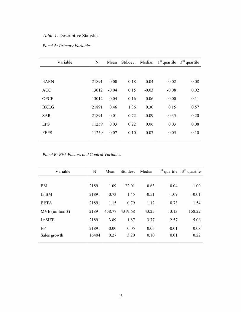
43

Table 1. Descriptive Statistics

Panel A: Primary Variables

Variable N Mean Std.dev. Median 1st quartile 3rd quartile EARN 21891 0.00 0.18 0.04 -0.02 0.08

ACC 13012 -0.04 0.15 -0.03 -0.08 0.02

OPCF 13012 0.04 0.16 0.06 -0.00 0.11

BKLG 21891 0.46 1.36 0.30 0.15 0.57

SAR 21891 0.01 0.72 -0.09 -0.35 0.20

EPS 11259 0.03 0.22 0.06 0.03 0.08

FEPS 11259 0.07 0.10 0.07 0.05 0.10

Panel B: Risk Factors and Control Variables

Variable N Mean Std.dev. Median 1st quartile 3rd quartile

BM 21891 1.09 22.01 0.63 0.04 1.00

LnBM 21891 -0.73 1.45 -0.51 -1.09 -0.01

BETA 21891 1.15 0.79 1.12 0.73 1.54

MVE (million $) 21891 458.77 4319.68 43.25 13.13 158.22

LnSIZE 21891 3.89 1.87 3.77 2.57 5.06

EP 21891 -0.00 0.05 0.05 -0.01 0.08Sales growth 16404 0.27 3.20 0.10 0.01 0.22

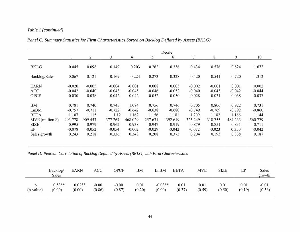
44

Table 1 (continued)

Panel C: Summary Statistics for Firm Characteristics Sorted on Backlog Deflated by Assets (BKLG)

Decile 1 2 3 4 5 6 7 8 9 10

BKLG 0.045 0.098 0.149 0.203 0.262 0.336 0.434 0.576 0.824 1.672 Backlog/Sales 0.067 0.121 0.169 0.224 0.273 0.328 0.420 0.541 0.720 1.312 EARN -0.020 -0.005 -0.004 -0.001 0.008 0.005 -0.002 -0.001 0.001 0.002 ACC -0.042 -0.040 -0.043 -0.045 -0.046 -0.052 -0.040 -0.043 -0.042 -0.044 OPCF 0.030 0.038 0.042 0.042 0.052 0.050 0.028 0.031 0.038 0.037 BM 0.781 0.740 0.745 1.084 0.756 0.746 0.705 0.806 0.922 0.731 LnBM -0.757 -0.711 -0.722 -0.642 -0.638 -0.680 -0.749 -0.769 -0.792 -0.860 BETA 1.107 1.115 1.123 1.162 1.156 1.181 1.209 1.182 1.166 1.144 MVE (million $) 493.778 909.453 377.267 468.029 257.631 392.619 325.249 318.755 484.233 560.779 SIZE 0.995 0.979 0.962 0.938 0.947 0.919 0.879 0.851 0.831 0.711 EP -0.078 -0.052 -0.054 -0.002 -0.029 -0.042 -0.072 -0.023 0.350 -0.042 Sales growth 0.243 0.218 0.336 0.348 0.208 0.373 0.204 0.193 0.338 0.187

Panel D: Pearson Correlation of Backlog Deflated by Assets (BKLG) with Firm Characteristics

Backlog/

Sales EARN ACC OPCF BM LnBM BETA MVE SIZE EP Sales

growth

ρ (p-value)

0.53** (0.00)

0.02** (0.00)

-0.00 (0.86)

-0.00 (0.87)

0.01 (0.20)

-0.03** (0.00)

0.01 (0.37)

0.01 (0.59)

0.01 (0.50)

0.01 (0.19)

-0.01 (0.56)

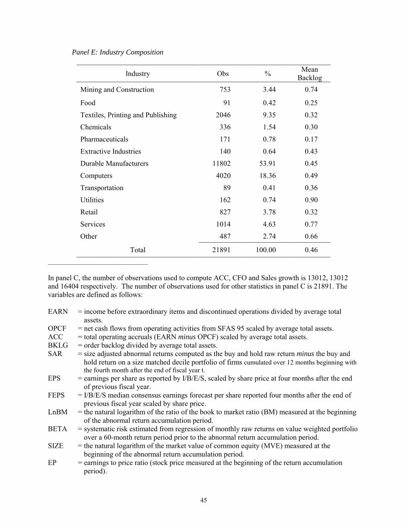
45

Panel E: Industry Composition

Industry Obs % Mean Backlog

Mining and Construction 753 3.44 0.74

Food 91 0.42 0.25

Textiles, Printing and Publishing 2046 9.35 0.32 Chemicals 336 1.54 0.30

Pharmaceuticals 171 0.78 0.17

Extractive Industries 140 0.64 0.43 Durable Manufacturers 11802 53.91 0.45

Computers 4020 18.36 0.49

Transportation 89 0.41 0.36 Utilities 162 0.74 0.90

Retail 827 3.78 0.32

Services 1014 4.63 0.77 Other 487 2.74 0.66

Total 21891 100.00 0.46 ______________________________ In panel C, the number of observations used to compute ACC, CFO and Sales growth is 13012, 13012 and 16404 respectively. The number of observations used for other statistics in panel C is 21891. The variables are defined as follows: EARN = income before extraordinary items and discontinued operations divided by average total

assets. OPCF = net cash flows from operating activities from SFAS 95 scaled by average total assets. ACC = total operating accruals (EARN minus OPCF) scaled by average total assets. BKLG = order backlog divided by average total assets. SAR = size adjusted abnormal returns computed as the buy and hold raw return minus the buy and

hold return on a size matched decile portfolio of firms cumulated over 12 months beginning with the fourth month after the end of fiscal year t.

EPS = earnings per share as reported by I/B/E/S, scaled by share price at four months after the end of previous fiscal year.

FEPS = I/B/E/S median consensus earnings forecast per share reported four months after the end of previous fiscal year scaled by share price.

LnBM = the natural logarithm of the ratio of the book to market ratio (BM) measured at the beginning of the abnormal return accumulation period.

BETA = systematic risk estimated from regression of monthly raw returns on value weighted portfolio over a 60-month return period prior to the abnormal return accumulation period.

SIZE = the natural logarithm of the market value of common equity (MVE) measured at the beginning of the abnormal return accumulation period.

EP = earnings to price ratio (stock price measured at the beginning of the return accumulation period).

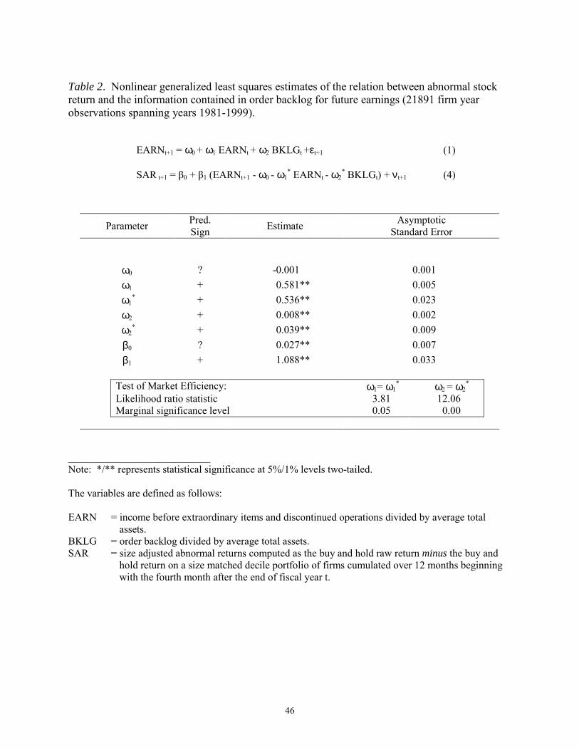
46

Table 2. Nonlinear generalized least squares estimates of the relation between abnormal stock return and the information contained in order backlog for future earnings (21891 firm year observations spanning years 1981-1999).

EARNt+1 = ω0 + ω1 EARNt + ω2 BKLGt +εt+1 (1)

SAR t+1 = β0 + β1 (EARNt+1 - ω0 - ω1* EARNt - ω2

* BKLGt) + νt+1 (4)

Parameter Pred. Sign Estimate Asymptotic

Standard Error

ω0 ? -0.001 0.001 ω1 + 0.581** 0.005

ω1* + 0.536** 0.023

ω2 + 0.008** 0.002 ω2

* + 0.039** 0.009 β0 ? 0.027** 0.007 β1 + 1.088** 0.033

Test of Market Efficiency: ω1= ω1* ω2 = ω2

* Likelihood ratio statistic 3.81 12.06 Marginal significance level 0.05 0.00

______________________________ Note: */** represents statistical significance at 5%/1% levels two-tailed. The variables are defined as follows: EARN = income before extraordinary items and discontinued operations divided by average total

assets. BKLG = order backlog divided by average total assets. SAR = size adjusted abnormal returns computed as the buy and hold raw return minus the buy and

hold return on a size matched decile portfolio of firms cumulated over 12 months beginning with the fourth month after the end of fiscal year t.

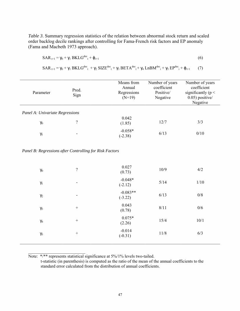
47

Table 3. Summary regression statistics of the relation between abnormal stock return and scaled order backlog decile rankings after controlling for Fama-French risk factors and EP anomaly (Fama and Macbeth 1973 approach).

SAR t+1 = γ0 + γ1 BKLGdec

t + ϕt+1 (6)

SAR t+1 = γ0 + γ1 BKLGdect + γ2 SIZEdec

t + γ3 BETAdect + γ4 LnBMdec

i + γ5 EPdeci + ϕt+1 (7)

Parameter Pred. Sign

Means from Annual

Regressions (N=19)

Number of years coefficient Positive/ Negative

Number of years coefficient

significantly (p < 0.05) positive/

Negative Panel A: Univariate Regressions

γ0 ? 0.042

(1.85) 12/7 3/3

γ1 - -0.058* (-2.38) 6/13 0/10

Panel B: Regressions after Controlling for Risk Factors

γ0 ? 0.027 (0.73) 10/9 4/2

γ1 - -0.048* (-2.12) 5/14 1/10

γ2 - -0.083**

(-3.22) 6/13 0/8

γ3 + 0.043 (0.78) 8/11 0/6

γ4 + 0.075* (2.26) 15/4 10/1

γ5 + -0.014 (-0.31) 11/8 6/3

_____________________________ Note: */** represents statistical significance at 5%/1% levels two-tailed. t-statistic (in parenthesis) is computed as the ratio of the mean of the annual coefficients to the standard error calculated from the distribution of annual coefficients.

48

Table 3 (continued) The variables are defined as follows: SAR = size adjusted abnormal returns computed as the buy and hold raw return minus the buy and

hold return on a size matched decile portfolio of firms cumulated over 12 months beginning with the fourth month after the end of fiscal year t.

BKLGdec = order backlog divided by average total assets, transformed to a scaled-decile variable with values ranging from 0 to 1.

SIZEdec = the natural logarithm of the market value of common equity measured at the beginning of the abnormal return accumulation period, transformed to a scaled-decile variable with values ranging from 0 to 1.

BETAdec = systematic risk estimated from regression of monthly raw returns on value weighted portfolio over a 60-month return period prior to the abnormal return accumulation period, transformed to a scaled-decile variable with values ranging from 0 to 1.

LnBMdec = the natural logarithm of the ratio of the book to market ratio measured at the beginning of the abnormal return accumulation period, transformed to a scaled-decile variable with values ranging from 0 to 1.

EPdec = earnings to price ratio (stock price measured at the beginning of the return accumulation period), transformed to a scaled-decile variable with values ranging from 0 to 1.

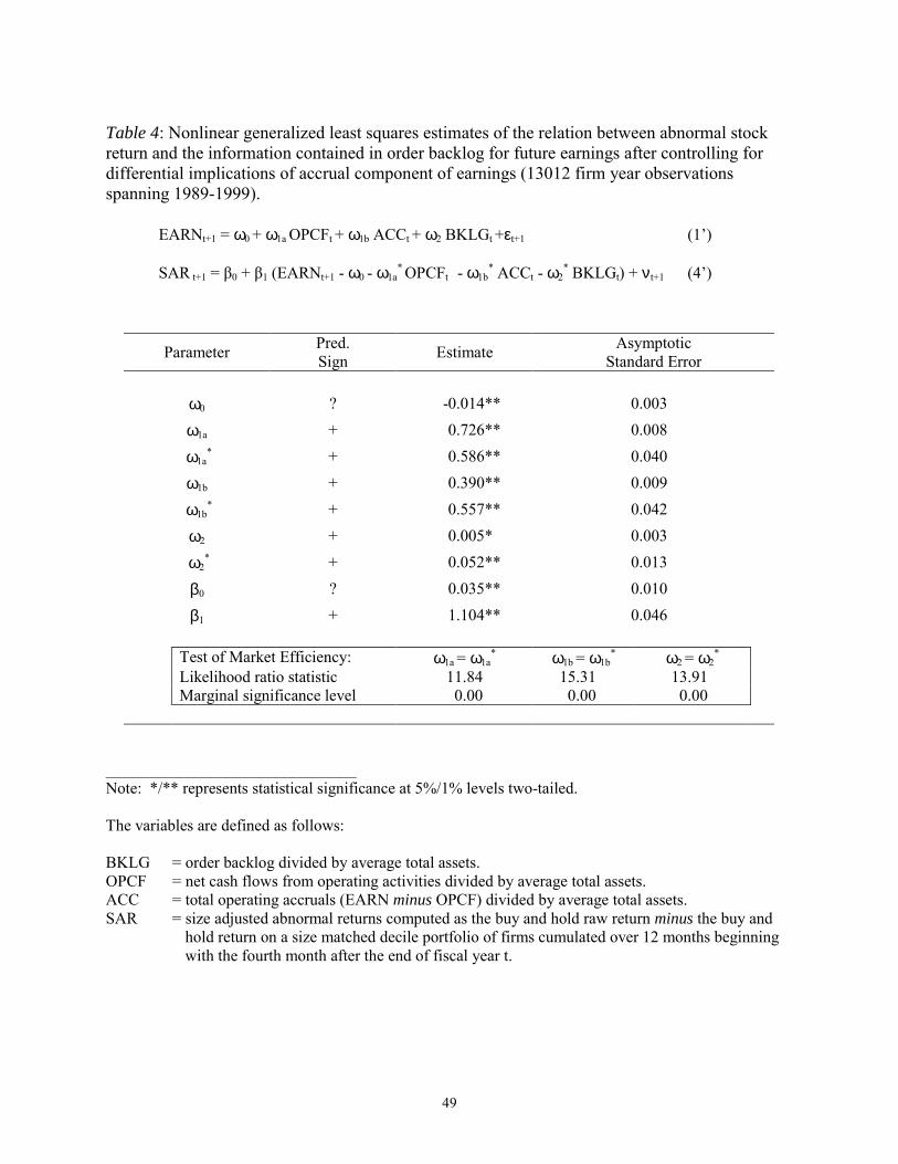
49

Table 4: Nonlinear generalized least squares estimates of the relation between abnormal stock return and the information contained in order backlog for future earnings after controlling for differential implications of accrual component of earnings (13012 firm year observations spanning 1989-1999). EARNt+1 = ω0 + ω1a OPCFt + ω1b ACCt + ω2 BKLGt +εt+1 (1�)

SAR t+1 = β0 + β1 (EARNt+1 - ω0 - ω1a* OPCFt - ω1b

* ACCt - ω2* BKLGt) + νt+1 (4�)

Parameter Pred. Sign Estimate Asymptotic

Standard Error

ω0 ? -0.014** 0.003

ω1a + 0.726** 0.008

ω1a* + 0.586** 0.040

ω1b + 0.390** 0.009

ω1b* + 0.557** 0.042

ω2 + 0.005* 0.003

ω2* + 0.052** 0.013

β0 ? 0.035** 0.010

β1 + 1.104** 0.046 Test of Market Efficiency: ω1a = ω1a

* ω1b = ω1b* ω2 = ω2

* Likelihood ratio statistic 11.84 15.31 13.91 Marginal significance level 0.00 0.00 0.00

_______________________________ Note: */** represents statistical significance at 5%/1% levels two-tailed. The variables are defined as follows: BKLG = order backlog divided by average total assets. OPCF = net cash flows from operating activities divided by average total assets. ACC = total operating accruals (EARN minus OPCF) divided by average total assets. SAR = size adjusted abnormal returns computed as the buy and hold raw return minus the buy and

hold return on a size matched decile portfolio of firms cumulated over 12 months beginning with the fourth month after the end of fiscal year t.

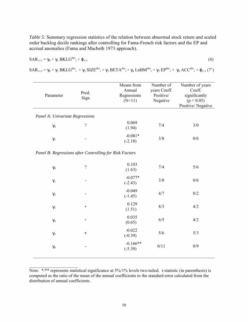
50

Table 5: Summary regression statistics of the relation between abnormal stock return and scaled order backlog decile rankings after controlling for Fama-French risk factors and the EP and accrual anomalies (Fama and Macbeth 1973 approach).

SAR t+1 = γ0 + γ1 BKLGdec

t + ϕt+1 (6) SAR t+1 = γ0 + γ1 BKLGdec

t + γ2 SIZEdect + γ3 BETAdec

t + γ4 LnBMdect + γ5 EPdec

t + γ6 ACCdect + ϕt+1 (7�)

Parameter Pred. Sign

Means from Annual

Regressions (N=11)

Number of years Coeff.

Positive/ Negative

Number of years Coeff.

significantly (p < 0.05)

Positive/ Negative Panel A: Univariate Regressions

γ0 ? 0.069 (1.94) 7/4 3/0

γ1 - -0.081* (-2.18) 3/8 0/6

Panel B: Regressions after Controlling for Risk Factors

γ0 ? 0.103 (1.63) 7/4 5/6

γ1 - -0.077* (-2.43) 3/8 0/6

γ2 - -0.049

(-1.45) 4/7 0/2

γ3 + 0.129 (1.51) 8/3 4/2

γ4 + 0.035 (0.65) 6/5 4/2

γ5 + -0.022 (-0.39) 5/6 5/3

γ6 - -0.166** (-5.30) 0/11 0/9

________________________ Note: */** represents statistical significance at 5%/1% levels two-tailed. t-statistic (in parenthesis) is computed as the ratio of the mean of the annual coefficients to the standard error calculated from the distribution of annual coefficients.

51

Table 5 (continued) The variables are defined as follows: SAR = size adjusted abnormal returns computed as the buy and hold raw return minus the buy and

hold return on a size matched decile portfolio of firms cumulated over 12 months beginning with the fourth month after the end of fiscal year t.

BKLGdec = order backlog divided by average total assets, transformed to a scaled-decile variable with values ranging from 0 to 1.

SIZEdec = the natural logarithm of the market value of common equity measured at the beginning of the abnormal return accumulation period, transformed to a scaled-decile variable with values ranging from 0 to 1.

BETAdec = systematic risk estimated from regression of monthly raw returns on value weighted portfolio over a 60-month return period prior to the abnormal return accumulation period, transformed to a scaled-decile variable with values ranging from 0 to 1.

LnBMdec = the natural logarithm of the ratio of the book to market ratio measured at the beginning of the abnormal return accumulation period, transformed to a scaled-decile variable with values ranging from 0 to 1.

EPdec = earnings to price ratio (stock price measured at the beginning of the return accumulation period), transformed to a scaled-decile variable with values ranging from 0 to 1.

ACCdec = total operating accruals (EARN minus OPCF) divided by average total assets, transformed to a scaled-decile variable with values ranging from 0 to 1.

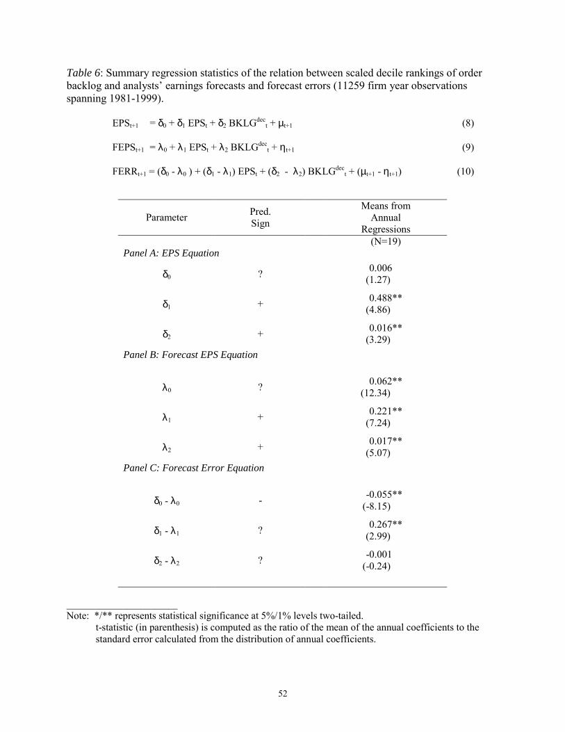
52

Table 6: Summary regression statistics of the relation between scaled decile rankings of order backlog and analysts� earnings forecasts and forecast errors (11259 firm year observations spanning 1981-1999).

EPSt+1 = δ0 + δ1 EPSt + δ2 BKLGdec

t + µt+1 (8) FEPSt+1 = λ0 + λ1 EPSt + λ2 BKLGdec

t + ηt+1 (9)

FERRt+1 = (δ0 - λ0 ) + (δ1 - λ1) EPSt + (δ2 - λ2) BKLGdect + (µt+1 - ηt+1) (10)

Parameter Pred. Sign

Means from Annual

Regressions (N=19) Panel A: EPS Equation

δ0 ? 0.006 (1.27)

δ1 + 0.488** (4.86)

δ2 + 0.016** (3.29)

Panel B: Forecast EPS Equation

λ0 ? 0.062** (12.34)

λ1 + 0.221** (7.24)

λ2 + 0.017** (5.07)

Panel C: Forecast Error Equation

δ0 - λ0 - -0.055** (-8.15)

δ1 - λ1 ? 0.267** (2.99)

δ2 - λ2 ? -0.001 (-0.24)

________________________ Note: */** represents statistical significance at 5%/1% levels two-tailed. t-statistic (in parenthesis) is computed as the ratio of the mean of the annual coefficients to the standard error calculated from the distribution of annual coefficients.

53

Table 6 (continued) The variables are defined as follows: EPS = earnings per share as reported by I/B/E/S, scaled by share price at four months after the end

of previous fiscal year. FEPS = I/B/E/S median consensus earnings forecast per share reported four months after the end of

previous fiscal year scaled by share price. FERR = forecast error computed as EPS minus FEPS. BKLGdec = order backlog divided by average total assets, transformed to a scaled-decile variable with

values ranging from 0 to 1.

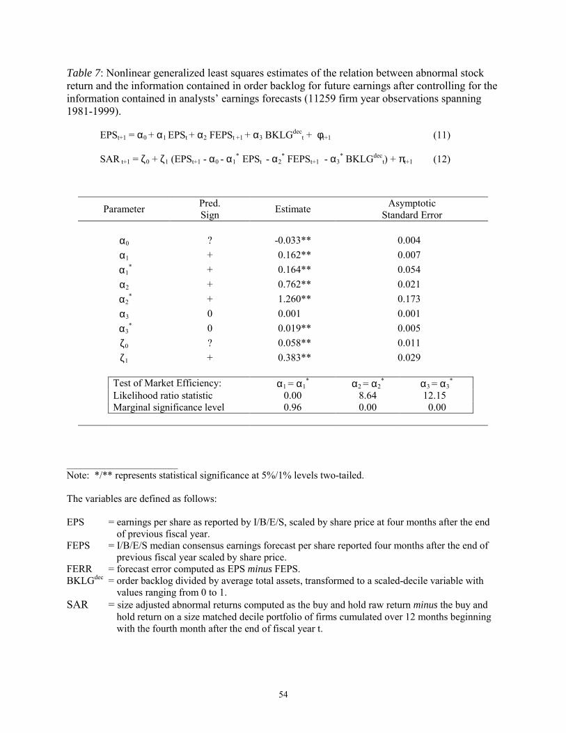
54

Table 7: Nonlinear generalized least squares estimates of the relation between abnormal stock return and the information contained in order backlog for future earnings after controlling for the information contained in analysts� earnings forecasts (11259 firm year observations spanning 1981-1999). EPSt+1 = α0 + α1 EPSt + α2 FEPSt +1 + α3 BKLGdec

t + φt+1 (11)

SAR t+1 = ζ0 + ζ1 (EPSt+1 - α0 - α1* EPSt - α2

* FEPSt+1 - α3* BKLGdec

t) + πt+1 (12)

Parameter Pred. Sign Estimate Asymptotic

Standard Error

α0 ? -0.033** 0.004 α1 + 0.162** 0.007

α1* + 0.164** 0.054

α2 + 0.762** 0.021 α2

* + 1.260** 0.173 α3 0 0.001 0.001

α3* 0 0.019** 0.005

ζ0 ? 0.058** 0.011 ζ1 + 0.383** 0.029

Test of Market Efficiency: α1 = α1

* α2 = α2* α3 = α3

* Likelihood ratio statistic 0.00 8.64 12.15 Marginal significance level 0.96 0.00 0.00

________________________ Note: */** represents statistical significance at 5%/1% levels two-tailed. The variables are defined as follows: EPS = earnings per share as reported by I/B/E/S, scaled by share price at four months after the end

of previous fiscal year. FEPS = I/B/E/S median consensus earnings forecast per share reported four months after the end of

previous fiscal year scaled by share price. FERR = forecast error computed as EPS minus FEPS. BKLGdec = order backlog divided by average total assets, transformed to a scaled-decile variable with

values ranging from 0 to 1. SAR = size adjusted abnormal returns computed as the buy and hold raw return minus the buy and

hold return on a size matched decile portfolio of firms cumulated over 12 months beginning with the fourth month after the end of fiscal year t.