Embed Size (px)
Citation preview
Does the Solow Model Explain the International Variation in the Standard of Living?
(Mankiw, Romer, Weil, QJE 1992)

Solow Model with Technological Progress
• Treat productivity (A term in our model) as due to level of technology.
• Assume that technology is labor-enhancing.
• So, can view labor input in terms of “effective units of labor.”
• Assume growth rate of technology is exogenous and equal to “g.”

Solow Model with Technological Progress
• Similar to way we modeled human capital, except now we assume this “quality” feature is due to technology.
• Later we will enter human capital into the model as a separate input.
• Specification allows production function to be expressed in terms of output per effective labor units and capital per effective labor units.
THE EMPIRICS OF ECONOMIC GROWTH 409
Finally, we discuss the predictions of the Solow model for international variation in rates of return and for capital move- ments. The model predicts that poor countries should tend to have higher rates of return to physical and human capital. We discuss various evidence that one might use to evaluate this prediction. In contrast to many recent authors, we interpret the available evidence on rates of return as generally consistent with the Solow model.
Overall, the findings reported in this paper cast doubt on the recent trend among economists to dismiss the Solow growth model in favor of endogenous-growth models that assume constant or increasing returns to scale in capital. One can explain much of the cross-country variation in income while maintaining the assump- tion of decreasing returns. This conclusion does not imply, how- ever, that the Solow model is a complete theory of growth: one would like also to understand the determinants of saving, popula- tion growth, and worldwide technological change, all of which the Solow model treats as exogenous. Nor does it imply that endogenous- growth models are not important, for they may provide the right explanation of worldwide technological change. Our conclusion does imply, however, that the Solow model gives the right answers to the questions it is designed to address.
I. THE TEXTBOOK SOLOW MODEL
We begin by briefly reviewing the Solow growth model. We focus on the model's implications for cross-country data.
A. The Model Solow's model takes the rates of saving, population growth,
and technological progress as exogenous. There are two inputs, capital and labor, which are paid their marginal products. We assume a Cobb-Douglas production function, so production at time t is given by
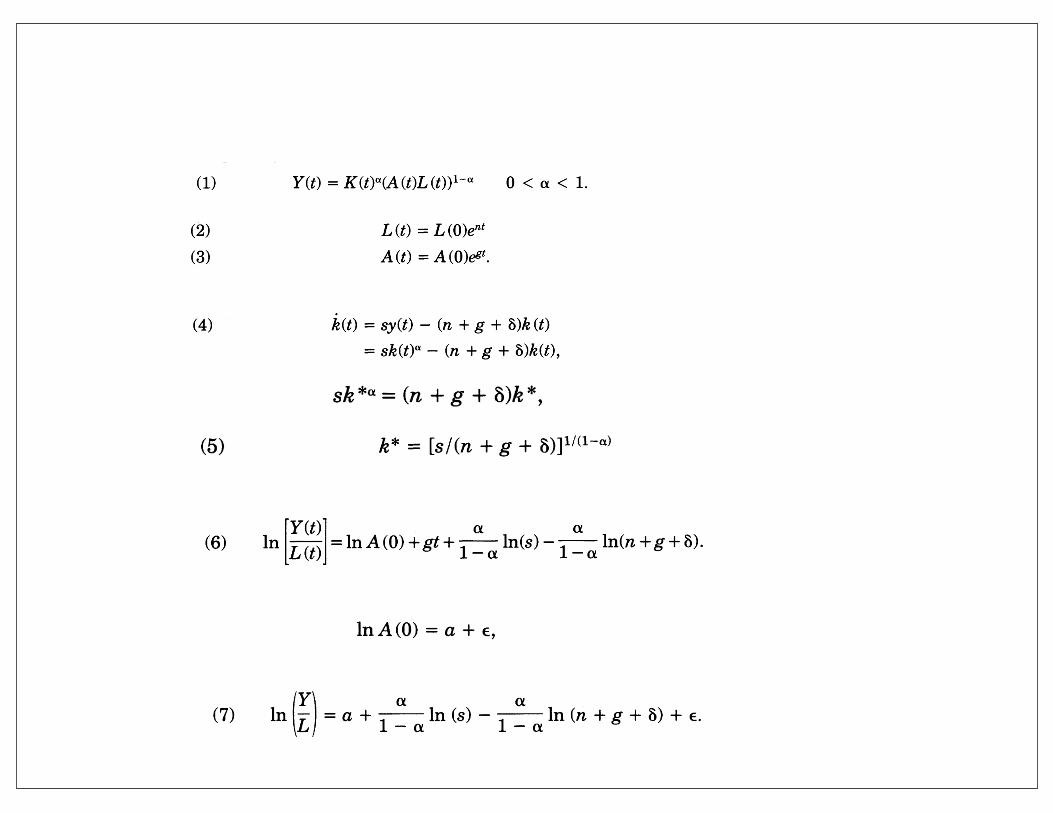
(1) Y(t) = K(t)a(A(t)L(t))l- 0 < a. < 1. The notation is standard: Y is output, K capital, L labor, and A the level of technology. L and A are assumed to grow exogenously at rates n and g:
(2) L (t) = L ()ent (3) A (t) = A (r)ent.
The number of effective units of labor, A (t)L (t), grows at rate n + g.
THE EMPIRICS OF ECONOMIC GROWTH 409
Finally, we discuss the predictions of the Solow model for international variation in rates of return and for capital move- ments. The model predicts that poor countries should tend to have higher rates of return to physical and human capital. We discuss various evidence that one might use to evaluate this prediction. In contrast to many recent authors, we interpret the available evidence on rates of return as generally consistent with the Solow model.
Overall, the findings reported in this paper cast doubt on the recent trend among economists to dismiss the Solow growth model in favor of endogenous-growth models that assume constant or increasing returns to scale in capital. One can explain much of the cross-country variation in income while maintaining the assump- tion of decreasing returns. This conclusion does not imply, how- ever, that the Solow model is a complete theory of growth: one would like also to understand the determinants of saving, popula- tion growth, and worldwide technological change, all of which the Solow model treats as exogenous. Nor does it imply that endogenous- growth models are not important, for they may provide the right explanation of worldwide technological change. Our conclusion does imply, however, that the Solow model gives the right answers to the questions it is designed to address.
I. THE TEXTBOOK SOLOW MODEL
We begin by briefly reviewing the Solow growth model. We focus on the model's implications for cross-country data.
A. The Model Solow's model takes the rates of saving, population growth,
and technological progress as exogenous. There are two inputs, capital and labor, which are paid their marginal products. We assume a Cobb-Douglas production function, so production at time t is given by
(1) Y(t) = K(t)a(A(t)L(t))l- 0 < a. < 1. The notation is standard: Y is output, K capital, L labor, and A the level of technology. L and A are assumed to grow exogenously at rates n and g:
(2) L (t) = L ()ent (3) A (t) = A (r)ent.
The number of effective units of labor, A (t)L (t), grows at rate n + g.
410 QUARTERLY JOURNAL OF ECONOMICS
The model assumes that a constant fraction of output, s, is invested. Defining k as the stock of capital per effective unit of labor, k = KIAL, and y as the level of output per effective unit of labor, y = Y/AL, the evolution of k is governed by
(4) k(t) = sy(t) - (n + g + 8)k (t) = sk(t)0 - (n + g + 8)k(t),
where 8 is the rate of depreciation. Equation (4) implies that k converges to a steady-state value k* defined by sk *a = (n + g + 8)k *, or
(5) k* = [s/(n + g + 5)]1I(1-a)
The steady-state capital-labor ratio is related positively to the rate of saving and negatively to the rate of population growth.
The central predictions of the Solow model concern the impact of saving and population growth on real income. Substituting (5) into the production function and taking logs, we find that steady- state income per capita is
(6)tl [Ot]ln()gt (6) In = In A (0) + gt + 1 In(s) - 1 ln(n + g + 8).
Because the model assumes that factors are paid their marginal products, it predicts not only the signs but also the magnitudes of the coefficients on saving and population growth. Specifically, because capital's share in income (a) is roughly one third, the model implies an elasticity of income per capita with respect to the saving rate of approximately 0.5 and an elasticity with respect to n + g + 8 of approximately -0.5.
B. Specification The natural question to consider is whether the data support
the Solow model's predictions concerning the determinants of standards of living. In other words, we want to investigate whether real income is higher in countries with higher saving rates and lower in countries with higher values of n + g + 5.
We assume that g and 8 are constant across countries. g reflects primarily the advancement of knowledge, which is not country-specific. And there is neither any strong reason to expect depreciation rates to vary greatly across countries, nor are there any data that would allow us to estimate country-specific deprecia- tion rates. In contrast, the A(0) term reflects not just technology
THE EMPIRICS OF ECONOMIC GROWTH 411
but resource endowments, climate, institutions, and so on; it may therefore differ across countries. We assume that
lnA(O) = a + E,
where a is a constant and E is a country-specific shock. Thus, log income per capita at a given time-time 0 for simplicity-is
(7) In a+ In(s)- In(n+g+8)+E.
Equation (7) is our basic empirical specification in this section. We assume that the rates of saving and population growth are
independent of country-specific factors shifting the production function. That is, we assume that s and n are independent of e. This assumption implies that we can estimate equation (7) with ordi- nary least squares (OLS).1
There are three reasons for making this assumption of indepen- dence. First, this assumption is made not only in the Solow model, but also in many standard models of economic growth. In any model in which saving and population growth are endogenous but preferences are isoelastic, s and n are unaffected by E. In other words, under isoelastic utility, permanent differences in the level of technology do not affect saving rates or population growth rates.
Second, much recent theoretical work on growth has been motivated by informal examinations of the relationships between saving, population growth, and income. Many economists have asserted that the Solow model cannot account for the international differences in income, and this alleged failure of the Solow model has stimulated work on endogenous-growth theory. For example, Romer [1987, 1989a] suggests that saving has too large an influence on growth and takes this to be evidence for positive externalities from capital accumulation. Similarly, Lucas [1988] asserts that variation in population growth cannot account for any substantial variation in real incomes along the lines predicted by the Solow model. By maintaining the identifying assumption that s and n are independent of E, we are able to determine whether systematic examination of the data confirms these informal judg- ments.
1. If s and n are endogenous and influenced by the level of income, then estimates of equation (7) using ordinary least squares are potentially inconsistent. In this case, to obtain consistent estimates, one needs to find instrumental variables that are correlated with s and n, but uncorrelated with the country-specific shift in the production function e. Finding such instrumental variables is a formidable task, however.
Solow Model with Technological Progress
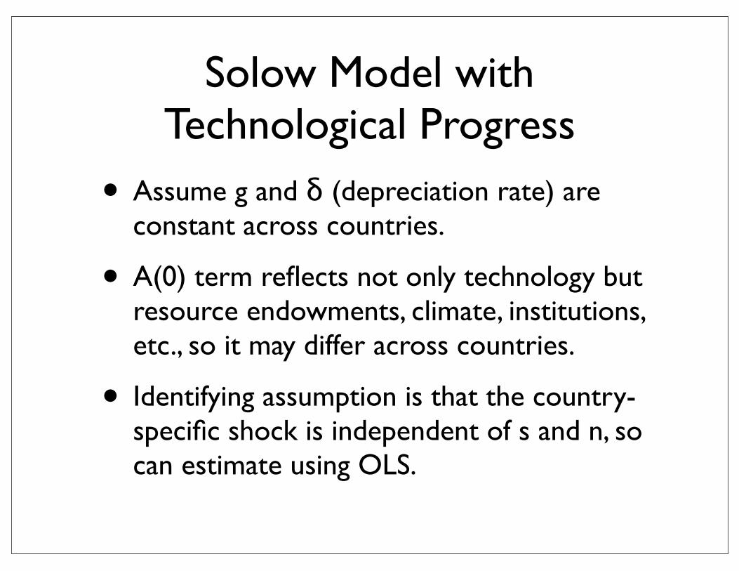
• Assume g and δ (depreciation rate) are constant across countries.
• A(0) term reflects not only technology but resource endowments, climate, institutions, etc., so it may differ across countries.
• Identifying assumption is that the country-specific shock is independent of s and n, so can estimate using OLS.
Solow Model with Technological Progress
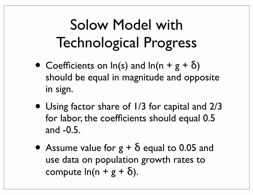
• Coefficients on ln(s) and ln(n + g + δ) should be equal in magnitude and opposite in sign.
• Using factor share of 1/3 for capital and 2/3 for labor, the coefficients should equal 0.5 and -0.5.
• Assume value for g + δ equal to 0.05 and use data on population growth rates to compute ln(n + g + δ).
Estimation Results forTextbook Solow Model
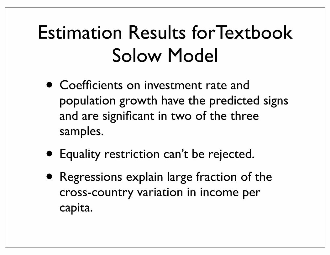
• Coefficients on investment rate and population growth have the predicted signs and are significant in two of the three samples.
• Equality restriction can’t be rejected.
• Regressions explain large fraction of the cross-country variation in income per capita.
414 QUARTERLY JOURNAL OF ECONOMICS
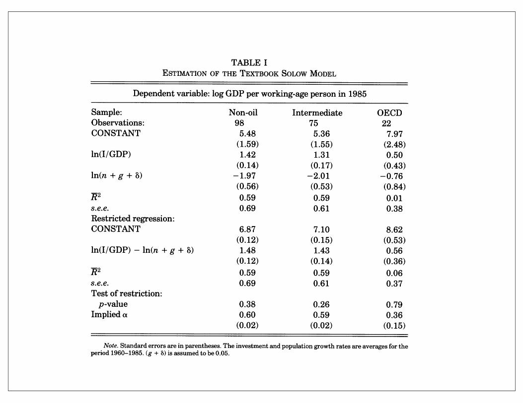
TABLE I ESTIMATION OF THE TEXTBOOK SOLOW MODEL
Dependent variable: log GDP per working-age person in 1985
Sample: Non-oil Intermediate OECD Observations: 98 75 22 CONSTANT 5.48 5.36 7.97
(1.59) (1.55) (2.48) ln(I/GDP) 1.42 1.31 0.50
(0.14) (0.17) (0.43) ln(n + g + 8) -1.97 -2.01 -0.76
(0.56) (0.53) (0.84) H2 0.59 0.59 0.01 s.e.e. 0.69 0.61 0.38 Restricted regression: CONSTANT 6.87 7.10 8.62
(0.12) (0.15) (0.53) ln(I/GDP) - ln(n + g + 8) 1.48 1.43 0.56
(0.12) (0.14) (0.36) 1?2 0.59 0.59 0.06 s.e.e. 0.69 0.61 0.37 Test of restriction:
p-value 0.38 0.26 0.79 Implied a 0.60 0.59 0.36
(0.02) (0.02) (0.15)
Note. Standard errors are in parentheses. The investment and population growth rates are averages for the period 1960-1985. (g + 8) is assumed to be 0.05.
Three aspects of the results support the Solow model. First, the coefficients on saving and population growth have the predicted signs and, for two of the three samples, are highly significant. Second, the restriction that the coefficients on ln(s) and ln(n + g + 8) are equal in magnitude and opposite in sign is not rejected in any of the samples. Third, and perhaps most important, differences in saving and population growth account for a large fraction of the cross-country variation in income per capita. In the regression for the intermediate sample, for example, the adjusted R2 is 0.59. In contrast to the common claim that the Solow model "explains" cross-country variation in labor productivity largely by appealing to variations in technologies, the two readily observable
about 0.03 or 0.04. In addition, growth in income per capita has averaged 1.7 percent per year in the United States and 2.2 percent per year in our intermediate sample; this suggests that g is about 0.02.
Estimation Results forTextbook Solow Model
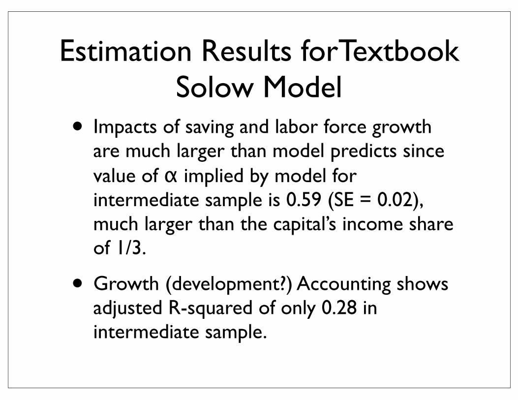
• Impacts of saving and labor force growth are much larger than model predicts since value of α implied by model for intermediate sample is 0.59 (SE = 0.02), much larger than the capital’s income share of 1/3.
• Growth (development?) Accounting shows adjusted R-squared of only 0.28 in intermediate sample.
Solow Model with Human Capital Accumulation
• Add human capital to production function.
• Include additional transition equation for adjustment of the stock of human capital.
• Solve for steady-state values of k and h.
416 QUARTERLY JOURNAL OF ECONOMICS
Table I human capital is an omitted variable. It is this empirical problem that we pursue in this section. We first expand the Solow model of Section I to include human capital. We show how leaving out human capital affects the coefficients on physical capital investment and population growth. We then run regressions analogous to those in Table I to see whether proxies for human capital can resolve the anomalies found in the first section.7
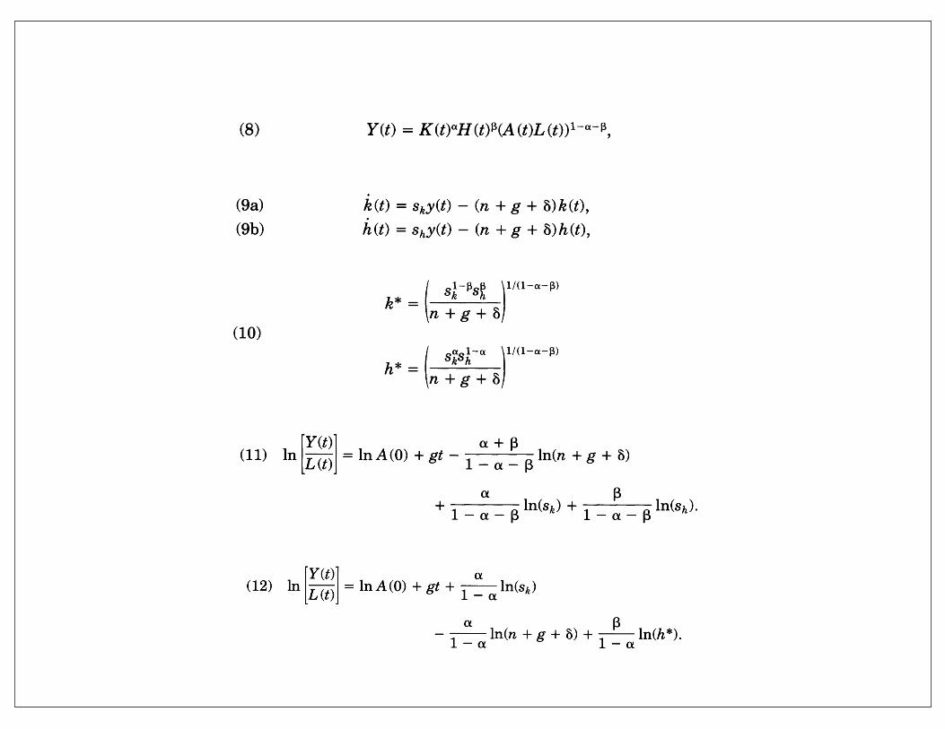
A. The Model Let the production function be
(8) Y(t) = K(t)H(t)P(A(t)L(t))1-a-, where H is the stock of human capital, and all other variables are defined as before. Let Sk be the fraction of income invested in physical capital and Sh the fraction invested in human capital. The evolution of the economy is determined by
(9a) k(t) = sky(t) - (n + g + 8)k(t), (9b) h(t) = Shy(t) - (n + g + 8)h(t),
where y = Y/AL, k = K/AL, and h = H/AL are quantities per effective unit of labor. We are assuming that the same production function applies to human capital, physical capital, and consump- tion. In other words, one unit of consumption can be transformed costlessly into either one unit of physical capital or one unit of human capital. In addition, we are assuming that human capital depreciates at the same rate as physical capital. Lucas [1988] models the production function for human capital as fundamen- tally different from that for other goods. We believe that, at least for an initial examination, it is natural to assume that the two types of production functions are similar.
We assume that a + ,B < 1, which implies that there are decreasing returns to all capital. (If a + ,B = 1, then there are constant returns to scale in the reproducible factors. In this case,
7. Previous authors have provided evidence of the importance of human capital for growth in income. Azariadis and Drazen [1990] find that no country was able to grow quickly during the postwar period without a highly literate labor force. They interpret this as evidence that there is a threshold externality associated with human capital accumulation. Similarly, Rauch [1988] finds that among countries that had achieved 95 percent adult literacy in 1960, there was a strong tendency for income per capita to converge over the period 1950-1985. Romer [1989b] finds that literacy in 1960 helps explain subsequent investment and that, if one corrects for measurement error, literacy has no impact on growth beyond its effect on investment. There is also older work stressing the role of human capital in development; for example, see Krueger [1968] and Easterlin [1981].
416 QUARTERLY JOURNAL OF ECONOMICS
Table I human capital is an omitted variable. It is this empirical problem that we pursue in this section. We first expand the Solow model of Section I to include human capital. We show how leaving out human capital affects the coefficients on physical capital investment and population growth. We then run regressions analogous to those in Table I to see whether proxies for human capital can resolve the anomalies found in the first section.7
A. The Model Let the production function be
(8) Y(t) = K(t)H(t)P(A(t)L(t))1-a-, where H is the stock of human capital, and all other variables are defined as before. Let Sk be the fraction of income invested in physical capital and Sh the fraction invested in human capital. The evolution of the economy is determined by
(9a) k(t) = sky(t) - (n + g + 8)k(t), (9b) h(t) = Shy(t) - (n + g + 8)h(t),
where y = Y/AL, k = K/AL, and h = H/AL are quantities per effective unit of labor. We are assuming that the same production function applies to human capital, physical capital, and consump- tion. In other words, one unit of consumption can be transformed costlessly into either one unit of physical capital or one unit of human capital. In addition, we are assuming that human capital depreciates at the same rate as physical capital. Lucas [1988] models the production function for human capital as fundamen- tally different from that for other goods. We believe that, at least for an initial examination, it is natural to assume that the two types of production functions are similar.
We assume that a + ,B < 1, which implies that there are decreasing returns to all capital. (If a + ,B = 1, then there are constant returns to scale in the reproducible factors. In this case,
7. Previous authors have provided evidence of the importance of human capital for growth in income. Azariadis and Drazen [1990] find that no country was able to grow quickly during the postwar period without a highly literate labor force. They interpret this as evidence that there is a threshold externality associated with human capital accumulation. Similarly, Rauch [1988] finds that among countries that had achieved 95 percent adult literacy in 1960, there was a strong tendency for income per capita to converge over the period 1950-1985. Romer [1989b] finds that literacy in 1960 helps explain subsequent investment and that, if one corrects for measurement error, literacy has no impact on growth beyond its effect on investment. There is also older work stressing the role of human capital in development; for example, see Krueger [1968] and Easterlin [1981].
THE EMPIRICS OF ECONOMIC GROWTH 417
there is no steady state for this model. We discuss this possibility in Section III.) Equations (9a) and (9b) imply that the economy converges to a steady state defined by
\n + g + (10)
(* a k -S a 1/(1-a-)
, n +g+ / Substituting (10) into the production function and taking logs gives an equation for income per capita similar to equation (6) above:
(1 1) In [L(t)| In A(O) + gt - + (I ln(n + g + a Y (t)]_
+ Iln(Sk) + In(Sh)
This equation shows how income per capita depends on population growth and accumulation of physical and human capital.
Like the textbook Solow model, the augmented model predicts coefficients in equation (11) that are functions of the factor shares. As before, a is physical capital's share of income, so we expect a value of a of about one third. Gauging a reasonable value of P, human capital's share, is more difficult. In the United States the minimum wage-roughly the return to labor without human capital-has averaged about 30 to 50 percent of the average wage in manufacturing. This fact suggests that 50 to 70 percent of total labor income represents the return to human capital, or that ,B is between one third and one half.
Equation (11) makes two predictions about the regressions run in Section I, in which human capital was ignored. First, even if In (Sh) is independent of the other right-hand side variables, the coefficient on ln(sk) is greater than a/(1 - a). For example, if a = P = 1/3, then the coefficient on ln(sk) would be 1. Because higher saving leads to higher income, it leads to a higher steady-state level of human capital, even if the percentage of income devoted to human-capital accumulation is unchanged. Hence, the presence of human-capital accumulation increases the impact of physical- capital accumulation on income.
Second, the coefficient on ln(n + g + 8) is larger in absolute
418 QUARTERLY JOURNAL OF ECONOMICS
value than the coefficient on ln(sk). If a =P = 1/3, for example, the coefficient on ln(n + g + 8) would be -2. In this model high population growth lowers income per capita because the amounts of both physical and human capital must be spread more thinly over the population.
There is an alternative way to express the role of human capital in determining income in this model. Combining (11) with the equation for the steady-state level of human capital given in (10) yields an equation for income as a function of the rate of investment in physical capital, the rate of population growth, and the level of human capital:
(12) In [L(t) = InA(O) + gt + 1 _ ln(sk)
aL Wi 1 -a n(n + g + 8) + - ln(h*).
Equation (12) is almost identical to equation (6) in Section I. In that model the level of human capital is a component of the error term. Because the saving and population growth rates influence h *, one should expect human capital to be positively correlated with the saving rate and negatively correlated with population growth. Therefore, omitting the human-capital term biases the coefficients on saving and population growth.
The model with human capital suggests two possible ways to modify our previous regressions. One way is to estimate the augmented model's reduced form, that is, equation (11), in which the rate of human-capital accumulation ln(sh) is added to the right-hand side. The second way is to estimate equation (12), in which the level of human capital In (h *) is added to the right-hand side. Notice that these alternative regressions predict different coefficients on the saving and population growth terms. When testing the augmented Solow model, a primary question is whether the available data on human capital correspond more closely to the rate of accumulation (Sh) or to the level of human capital (h).
B. Data To implement the model, we restrict our focus to human-
capital investment in the form of education-thus ignoring invest- ment in health, among other things. Despite this narrowed focus, measurement of human capital presents great practical difficulties. Most important, a large part of investment in education takes the
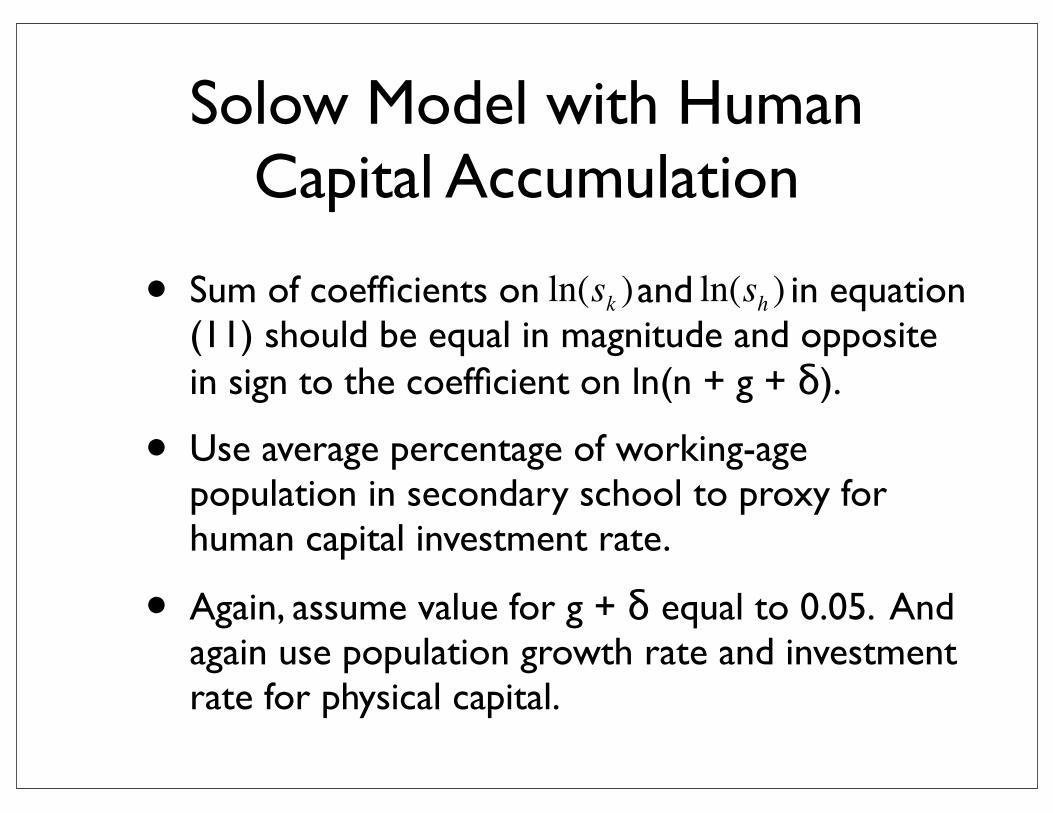
Solow Model with Human Capital Accumulation
• Sum of coefficients on and in equation (11) should be equal in magnitude and opposite in sign to the coefficient on ln(n + g + δ).
• Use average percentage of working-age population in secondary school to proxy for human capital investment rate.
• Again, assume value for g + δ equal to 0.05. And again use population growth rate and investment rate for physical capital.
ln(sk ) ln(sh )
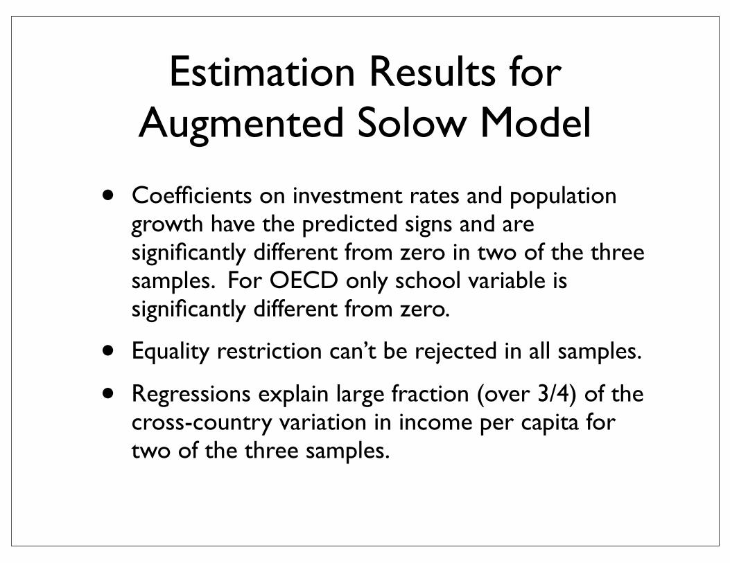
Estimation Results for Augmented Solow Model
• Coefficients on investment rates and population growth have the predicted signs and are significantly different from zero in two of the three samples. For OECD only school variable is significantly different from zero.
• Equality restriction can’t be rejected in all samples.
• Regressions explain large fraction (over 3/4) of the cross-country variation in income per capita for two of the three samples.
420 QUARTERLY JOURNAL OF ECONOMICS
and I/GDP is 0.59 for the intermediate sample, and the correlation between SCHOOL and the population growth rate is -0.38. Thus, including human-capital accumulation could alter substantially the estimated impact of physical-capital accumulation and popula- tion growth on income per capita.
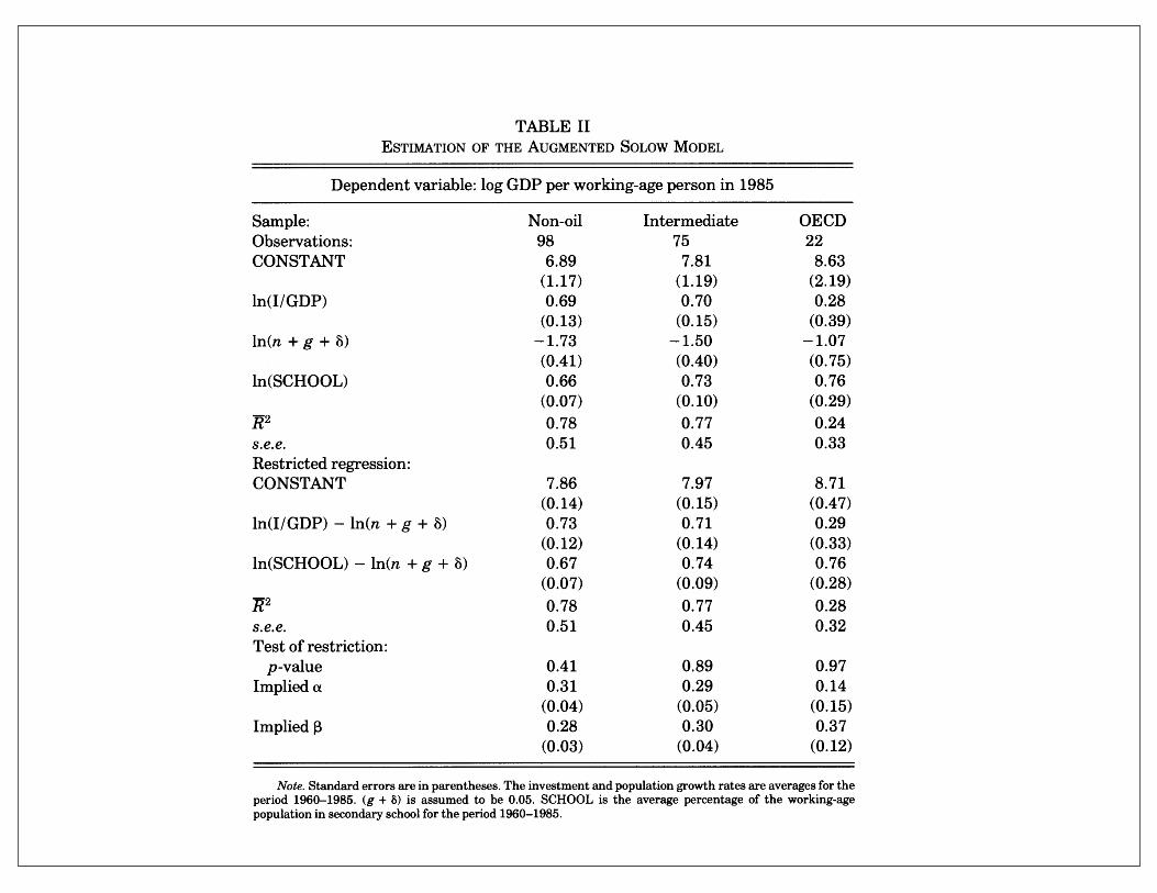
C. Results Table II presents regressions of the log of income per capita on
the log of the investment rate, the log of n + g + 8, and the log of the percentage of the population in secondary school. The human- capital measure enters significantly in all three samples. It also
TABLE II ESTIMATION OF THE AUGMENTED SOLOW MODEL
Dependent variable: log GDP per working-age person in 1985
Sample: Non-oil Intermediate OECD Observations: 98 75 22 CONSTANT 6.89 7.81 8.63
(1.17) (1.19) (2.19) ln(I/GDP) 0.69 0.70 0.28
(0.13) (0.15) (0.39) ln(n + g + 5) -1.73 -1.50 -1.07
(0.41) (0.40) (0.75) ln(SCHOOL) 0.66 0.73 0.76
(0.07) (0.10) (0.29) R2 0.78 0.77 0.24 s.e.e. 0.51 0.45 0.33 Restricted regression: CONSTANT 7.86 7.97 8.71
(0.14) (0.15) (0.47) ln(I/GDP) - ln(n + g + 5) 0.73 0.71 0.29
(0.12) (0.14) (0.33) ln(SCHOOL) - ln(n + g + 5) 0.67 0.74 0.76
(0.07) (0.09) (0.28) R2 0.78 0.77 0.28 s.e.e. 0.51 0.45 0.32 Test of restriction:
p-value 0.41 0.89 0.97 Implied a 0.31 0.29 0.14
(0.04) (0.05) (0.15) Implied , 0.28 0.30 0.37
(0.03) (0.04) (0.12)
Note. Standard errors are in parentheses. The investment and population growth rates are averages for the period 1960-1985. (g + 8) is assumed to be 0.05. SCHOOL is the average percentage of the working-age population in secondary school for the period 1960-1985.
Estimation Results for Augmented Solow Model
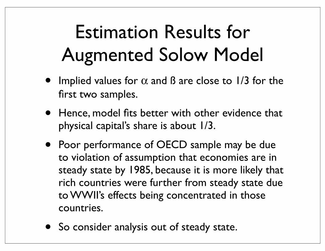
• Implied values for α and ß are close to 1/3 for the first two samples.
• Hence, model fits better with other evidence that physical capital’s share is about 1/3.
• Poor performance of OECD sample may be due to violation of assumption that economies are in steady state by 1985, because it is more likely that rich countries were further from steady state due to WWII’s effects being concentrated in those countries.
• So consider analysis out of steady state.
Convergence to Steady State
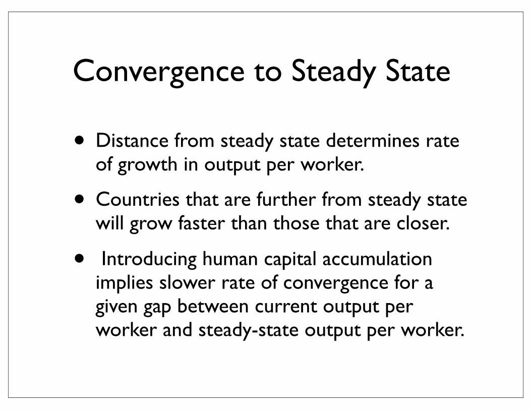
• Distance from steady state determines rate of growth in output per worker.
• Countries that are further from steady state will grow faster than those that are closer.
• Introducing human capital accumulation implies slower rate of convergence for a given gap between current output per worker and steady-state output per worker.
THE EMPIRICS OF ECONOMIC GROWTH 423
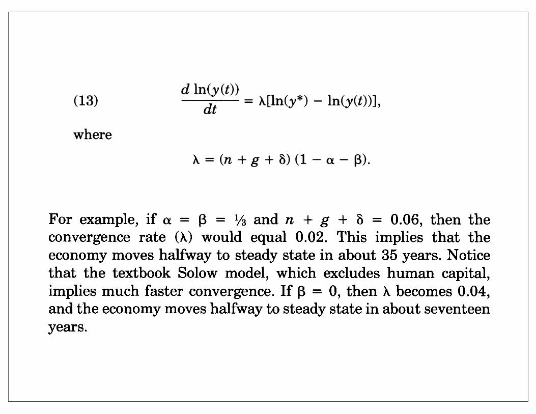
For example, if a = P = 1/3 and n + g + 8 = 0.06, then the convergence rate (A) would equal 0.02. This implies that the economy moves halfway to steady state in about 35 years. Notice that the textbook Solow model, which excludes human capital, implies much faster convergence. If IB = 0, then X becomes 0.04, and the economy moves halfway to steady state in about seventeen years.
The model suggests a natural regression to study the rate of convergence. Equation (13) implies that
(14) ln(y(t)) = (1 - e-At) ln(y*) + e-At ln(y(0)),
where y(O) is income per effective worker at some initial date. Subtracting In (y(O)) from both sides, (15) ln(y(t)) - ln(y(0)) = (1 - e-t) ln(y*) - (1 - e-At) ln(y(0)).
Finally, substituting for y*:
(16) ln(y(t)) - ln(y(0)) = (1 - e-t) ln(sk)
+ (1 - e-t) ln(sh)
- (1 - eAxt) l _ _ In(n + g + 8) - (1 - e-t) ln(y(0)).
Thus, in the Solow model the growth of income is a function of the determinants of the ultimate steady state and the initial level of income.
Endogenous-growth models make predictions very different from the Solow model regarding convergence among countries. In endogenous-growth models there is no steady-state level of income; differences among countries in income per capita can persist indefinitely, even if the countries have the same saving and population growth rates.12 Endogenous-growth models with a
12. Although we do not explore the issue here, endogenous-growth models also make quantitative predictions about the impact of saving on growth. The models are typically characterized by constant returns to reproducible factors of production, namely physical and human capital. Our model of Section II with a + , = 1 and g = 0 provides a simple way of analyzing the predictions of models of endogenous growth. With these modifications to the model of Section II, the production function is Y = AKaH1-a. In this form the model predicts that the ratio of physical to human capital, K/H, will converge to SkiSh, and that K, H, and Y will then all grow at rate A(Sk)a(Sh )'-a. The derivative of this "steady-state" growth rate with respect to Sk is then aA(ShlSk) 1- = atI(KIY). The impact of saving on growth depends on the
422 QUARTERLY JOURNAL OF ECONOMICS
Advocates of endogenous-growth models present them as alternatives to the Solow model and motivate them by an alleged empirical failure of the Solow model to explain cross-country differences. Barro [1989] presents the argument succinctly: In neoclassical growth models with diminishing returns, such as Solow (1956), Cass (1965) and Koopmans (1965), a country's per capita growth rate tends to be inversely related to its starting level of income per person. Therefore, in the absence of shocks, poor and rich countries would tend to converge in terms of levels of per capita income. However, this convergence hypothesis seems to be inconsistent with the cross-country evidence, which indicates that per capita growth rates are uncorrelated with the starting level of per capita product.
Our first goal in this section is to reexamine this evidence on convergence to assess whether it contradicts the Solow model.
Our second goal is to generalize our previous results. To implement the Solow model, we have been assuming that countries in 1985 were in their steady states (or, more generally, that the deviations from steady state were random). Yet this assumption is questionable. We therefore examine the predictions of the aug- mented Solow model for behavior out of the steady state.
A. Theory The Solow model predicts that countries reach different steady
states. In Section II we argued that much of the cross-country differences in income per capita can be traced to differing determi- nants of the steady state in the Solow growth model: accumulation of human and physical capital and population growth. Thus, the Solow model does not predict convergence; it predicts only that income per capita in a given country converges to that country's steady-state value. In other words, the Solow model predicts convergence only after controlling for the determinants of the steady state, a phenomenon that might be called "conditional convergence."
In addition, the Solow model makes quantitative predictions about the speed of convergence to steady state. Let y * be the steady-state level of income per effective worker given by equation (11), and let y(t) be the actual value at time t. Approximating around the steady state, the speed of convergence is given by
d ln(y(t)) (13) dt = X[ln(y*) -ln(y(t))],
where
A = (n + g + a) (1-a -
Convergence to Steady State
• Equation (13) can be used to derive an estimating equation to test for convergence.
• This leads to an equation that expresses growth in output per worker as a function of the steady state and the initial level of output per worker:
422 QUARTERLY JOURNAL OF ECONOMICS
Advocates of endogenous-growth models present them as alternatives to the Solow model and motivate them by an alleged empirical failure of the Solow model to explain cross-country differences. Barro [1989] presents the argument succinctly: In neoclassical growth models with diminishing returns, such as Solow (1956), Cass (1965) and Koopmans (1965), a country's per capita growth rate tends to be inversely related to its starting level of income per person. Therefore, in the absence of shocks, poor and rich countries would tend to converge in terms of levels of per capita income. However, this convergence hypothesis seems to be inconsistent with the cross-country evidence, which indicates that per capita growth rates are uncorrelated with the starting level of per capita product.
Our first goal in this section is to reexamine this evidence on convergence to assess whether it contradicts the Solow model.
Our second goal is to generalize our previous results. To implement the Solow model, we have been assuming that countries in 1985 were in their steady states (or, more generally, that the deviations from steady state were random). Yet this assumption is questionable. We therefore examine the predictions of the aug- mented Solow model for behavior out of the steady state.
A. Theory The Solow model predicts that countries reach different steady
states. In Section II we argued that much of the cross-country differences in income per capita can be traced to differing determi- nants of the steady state in the Solow growth model: accumulation of human and physical capital and population growth. Thus, the Solow model does not predict convergence; it predicts only that income per capita in a given country converges to that country's steady-state value. In other words, the Solow model predicts convergence only after controlling for the determinants of the steady state, a phenomenon that might be called "conditional convergence."
In addition, the Solow model makes quantitative predictions about the speed of convergence to steady state. Let y * be the steady-state level of income per effective worker given by equation (11), and let y(t) be the actual value at time t. Approximating around the steady state, the speed of convergence is given by
d ln(y(t)) (13) dt = X[ln(y*) -ln(y(t))],
where
A = (n + g + a) (1-a -
THE EMPIRICS OF ECONOMIC GROWTH 423
For example, if a = P = 1/3 and n + g + 8 = 0.06, then the convergence rate (A) would equal 0.02. This implies that the economy moves halfway to steady state in about 35 years. Notice that the textbook Solow model, which excludes human capital, implies much faster convergence. If IB = 0, then X becomes 0.04, and the economy moves halfway to steady state in about seventeen years.
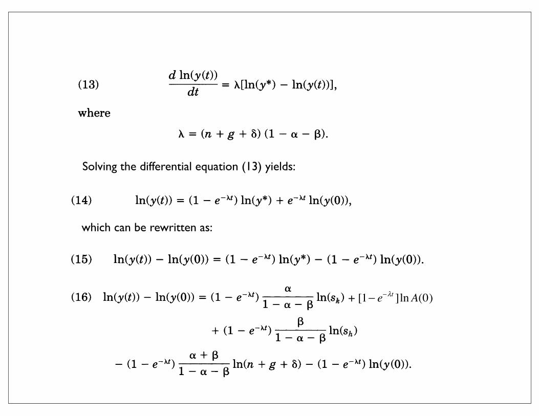
The model suggests a natural regression to study the rate of convergence. Equation (13) implies that
(14) ln(y(t)) = (1 - e-At) ln(y*) + e-At ln(y(0)),
where y(O) is income per effective worker at some initial date. Subtracting In (y(O)) from both sides, (15) ln(y(t)) - ln(y(0)) = (1 - e-t) ln(y*) - (1 - e-At) ln(y(0)).
Finally, substituting for y*:
(16) ln(y(t)) - ln(y(0)) = (1 - e-t) ln(sk)
+ (1 - e-t) ln(sh)
- (1 - eAxt) l _ _ In(n + g + 8) - (1 - e-t) ln(y(0)).
Thus, in the Solow model the growth of income is a function of the determinants of the ultimate steady state and the initial level of income.
Endogenous-growth models make predictions very different from the Solow model regarding convergence among countries. In endogenous-growth models there is no steady-state level of income; differences among countries in income per capita can persist indefinitely, even if the countries have the same saving and population growth rates.12 Endogenous-growth models with a
12. Although we do not explore the issue here, endogenous-growth models also make quantitative predictions about the impact of saving on growth. The models are typically characterized by constant returns to reproducible factors of production, namely physical and human capital. Our model of Section II with a + , = 1 and g = 0 provides a simple way of analyzing the predictions of models of endogenous growth. With these modifications to the model of Section II, the production function is Y = AKaH1-a. In this form the model predicts that the ratio of physical to human capital, K/H, will converge to SkiSh, and that K, H, and Y will then all grow at rate A(Sk)a(Sh )'-a. The derivative of this "steady-state" growth rate with respect to Sk is then aA(ShlSk) 1- = atI(KIY). The impact of saving on growth depends on the
THE EMPIRICS OF ECONOMIC GROWTH 423
For example, if a = P = 1/3 and n + g + 8 = 0.06, then the convergence rate (A) would equal 0.02. This implies that the economy moves halfway to steady state in about 35 years. Notice that the textbook Solow model, which excludes human capital, implies much faster convergence. If IB = 0, then X becomes 0.04, and the economy moves halfway to steady state in about seventeen years.
The model suggests a natural regression to study the rate of convergence. Equation (13) implies that
(14) ln(y(t)) = (1 - e-At) ln(y*) + e-At ln(y(0)),
where y(O) is income per effective worker at some initial date. Subtracting In (y(O)) from both sides, (15) ln(y(t)) - ln(y(0)) = (1 - e-t) ln(y*) - (1 - e-At) ln(y(0)).
Finally, substituting for y*:
(16) ln(y(t)) - ln(y(0)) = (1 - e-t) ln(sk)
+ (1 - e-t) ln(sh)
- (1 - eAxt) l _ _ In(n + g + 8) - (1 - e-t) ln(y(0)).
Thus, in the Solow model the growth of income is a function of the determinants of the ultimate steady state and the initial level of income.
Endogenous-growth models make predictions very different from the Solow model regarding convergence among countries. In endogenous-growth models there is no steady-state level of income; differences among countries in income per capita can persist indefinitely, even if the countries have the same saving and population growth rates.12 Endogenous-growth models with a
12. Although we do not explore the issue here, endogenous-growth models also make quantitative predictions about the impact of saving on growth. The models are typically characterized by constant returns to reproducible factors of production, namely physical and human capital. Our model of Section II with a + , = 1 and g = 0 provides a simple way of analyzing the predictions of models of endogenous growth. With these modifications to the model of Section II, the production function is Y = AKaH1-a. In this form the model predicts that the ratio of physical to human capital, K/H, will converge to SkiSh, and that K, H, and Y will then all grow at rate A(Sk)a(Sh )'-a. The derivative of this "steady-state" growth rate with respect to Sk is then aA(ShlSk) 1- = atI(KIY). The impact of saving on growth depends on the
+ [1− e−λt ]lnA(0)
Solving the differential equation (13) yields:
which can be rewritten as:
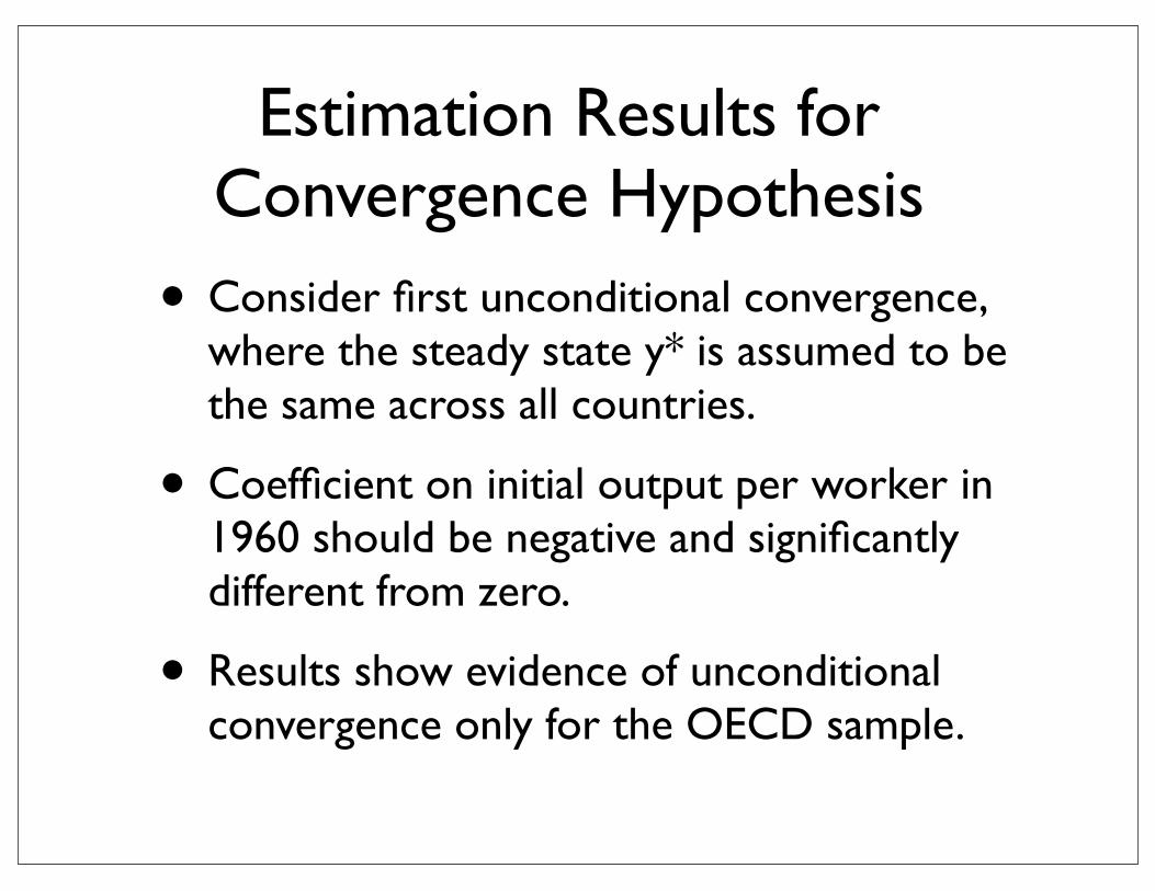
Estimation Results for Convergence Hypothesis
• Consider first unconditional convergence, where the steady state y* is assumed to be the same across all countries.
• Coefficient on initial output per worker in 1960 should be negative and significantly different from zero.
• Results show evidence of unconditional convergence only for the OECD sample.
THE EMPIRICS OF ECONOMIC GROWTH 425
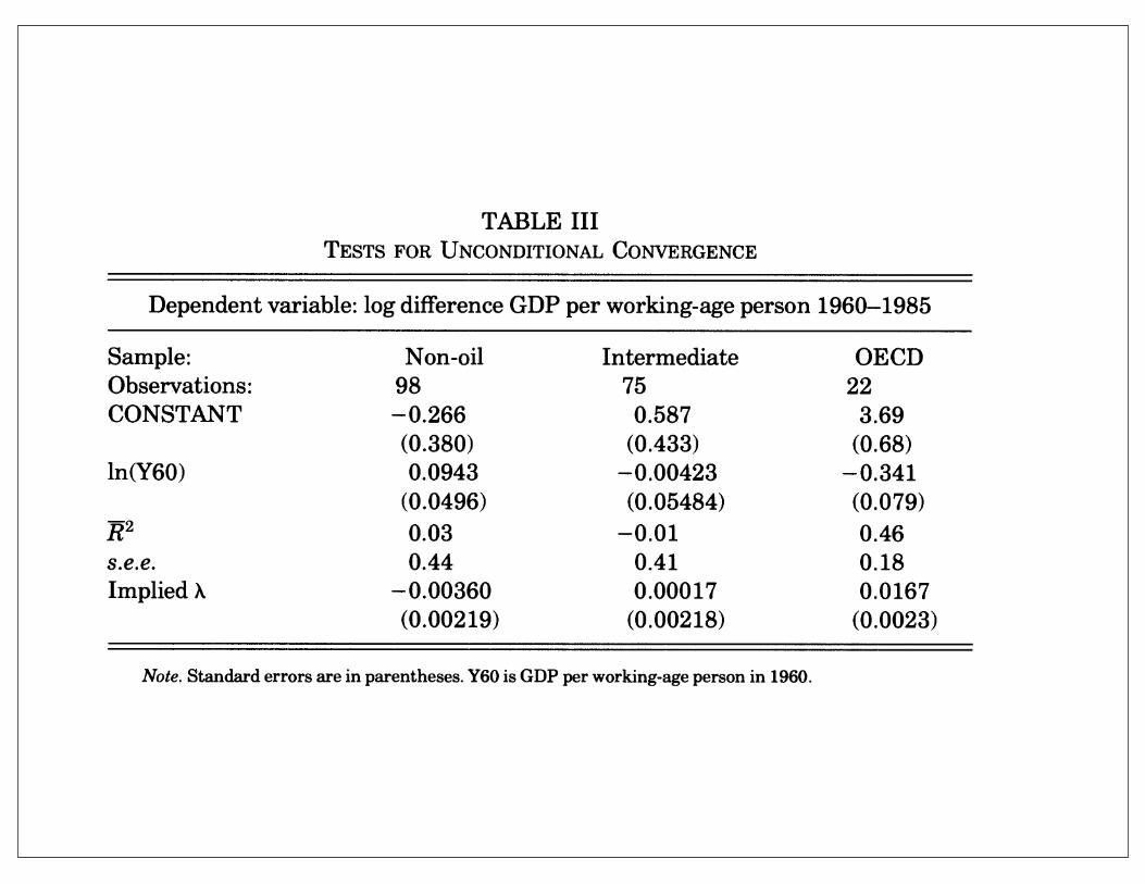
TABLE III TESTS FOR UNCONDITIONAL CONVERGENCE
Dependent variable: log difference GDP per working-age person 1960-1985
Sample: Non-oil Intermediate OECD Observations: 98 75 22 CONSTANT -0.266 0.587 3.69
(0.380) (0.433) (0.68) ln(Y60) 0.0943 -0.00423 -0.341
(0.0496) (0.05484) (0.079) R2 0.03 -0.01 0.46 s.e.e. 0.44 0.41 0.18 Implied X -0.00360 0.00017 0.0167
(0.00219) (0.00218) (0.0023)
Note. Standard errors are in parentheses. Y60 is GDP per working-age person in 1960.
essentially zero. There is no tendency for poor countries to grow faster on average than rich countries.
Table III does show, however, that there is a significant tendency toward convergence in the OECD sample. The coefficient on the initial level of income per capita is significantly negative, and the adjusted R2 of the regression is 0.46. This result confirms the findings of Dowrick and Nguyen [1989], among others.
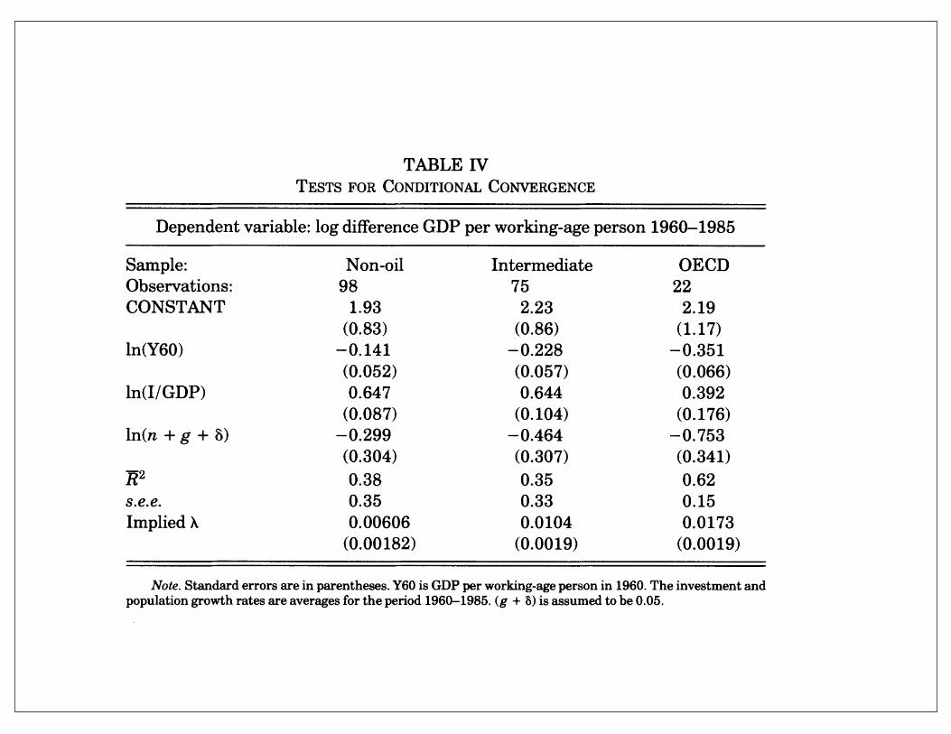
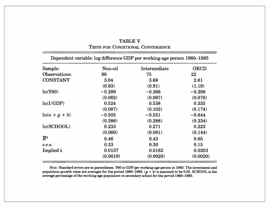
Table IV adds our measures of the rates of investment and population growth to the right-hand side of the regression. In all three samples the coefficient on the initial level of income is now significantly negative; that is, there is strong evidence of conver- gence. Moreover, the inclusion of investment and population growth rates improves substantially the fit of the regression. Table V adds our measure of human capital to the right-hand side of the regression in Table IV. This new variable further lowers the coefficient on the initial level of income, and it again improves the fit of the regression.
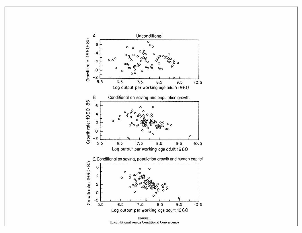
Figure I presents a graphical demonstration of the effect of adding measures of population growth and accumulation of human and physical capital to the usual "convergence picture," first presented by Romer [1987]. The top panel presents a scatterplot for our intermediate sample of the average annual growth rate of income per capita from 1960 to 1985 against the log of income per capita in 1960. Clearly, there is no evidence that countries that start off poor tend to grow faster. The second panel of the figure
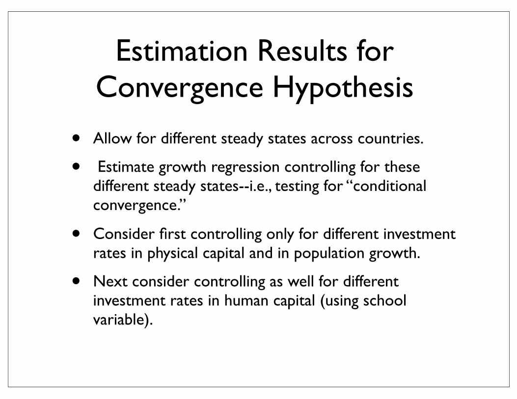
Estimation Results for Convergence Hypothesis
• Allow for different steady states across countries.
• Estimate growth regression controlling for these different steady states--i.e., testing for “conditional convergence.”
• Consider first controlling only for different investment rates in physical capital and in population growth.
• Next consider controlling as well for different investment rates in human capital (using school variable).
426 QUARTERLY JOURNAL OF ECONOMICS
TABLE IV TESTS FOR CONDITIONAL CONVERGENCE
Dependent variable: log difference GDP per working-age person 1960-1985
Sample: Non-oil Intermediate OECD Observations: 98 75 22 CONSTANT 1.93 2.23 2.19
(0.83) (0.86) (1.17) ln(Y60) -0.141 -0.228 -0.351
(0.052) (0.057) (0.066) ln(I/GDP) 0.647 0.644 0.392
(0.087) (0.104) (0.176) ln(n + g + 8) -0.299 -0.464 -0.753
(0.304) (0.307) (0.341) R72 0.38 0.35 0.62 s.e.e. 0.35 0.33 0.15 Implied X 0.00606 0.0104 0.0173
(0.00182) (0.0019) (0.0019)
Note. Standard errors are in parentheses. Y60 is GDP per working-age person in 1960. The investment and population growth rates are averages for the period 1960-1985. (g + 8) is assumed to be 0.05.
TABLE V TESTS FOR CONDITIONAL CONVERGENCE
Dependent variable: log difference GDP per working-age person 1960-1985
Sample: Non-oil Intermediate OECD Observations: 98 75 22 CONSTANT 3.04 3.69 2.81
(0.83) (0.91) (1.19) ln(Y60) -0.289 -0.366 -0.398
(0.062) (0.067) (0.070) ln(I/GDP) 0.524 0.538 0.335
(0.087) (0.102) (0.174) ln(n + g + 8) -0.505 -0.551 -0.844
(0.288) (0.288) (0.334) ln(SCHOOL) 0.233 0.271 0.223
(0.060) (0.081) (0.144) R2 0.46 0.43 0.65 s.e.e. 0.33 0.30 0.15 Implied X 0.0137 0.0182 0.0203
(0.0019) (0.0020) (0.0020)
Note. Standard errors are in parentheses. Y60 is GDP per working-age person in 1960. The investment and population growth rates are averages for the period 1960-1985. (g + 8) is assumed to be 0.05. SCHOOL is the average percentage of the working-age population in secondary school for the period 1960-1985.
THE EMPIRICS OF ECONOMIC GROWTH 427
A. Unconditional co 6 0 6 0 0 00 (0 ~~~~~0 0 Q) 4 Oo
R 0 0O 0 -- ~~00 0 0
2 2 o ? 0 o
-~0 0 Oo0 00 ? -2 s 5,5 6,5 7,5 8,5 9.5 10.5
Log output per working age adult: 1960
B. Conditional on saving and population growth 6 ~~ ~~0 0
060 0 0 o0c~ 08 W, 4 _CP O? ?? ?0 8
= 2 0 o D 0
o 020 0
5 s,5 6.5 7, 5 8.5 9.5 10,5 Log output per working age adult:1960
C. Conditional on saving, population growth and human capital LO
6 0 0 0~~~~~~
2 - ? ? O??b 9 lb8 0~~~~~~
? -2 w 5.5 6.5 7.5 8.5 9.5 10.5
Log output per working age adult: 1960 FIGURE I
Unconditional versus Conditional Convergence
Estimation Results for Convergence Hypothesis
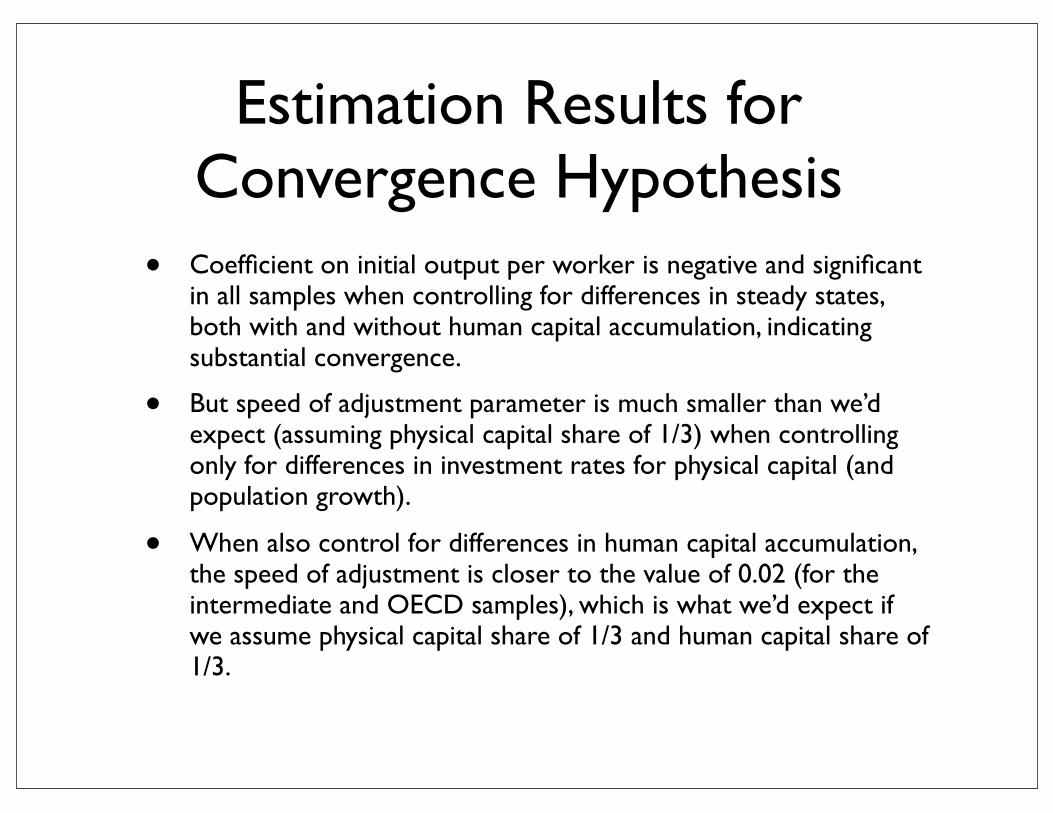
• Coefficient on initial output per worker is negative and significant in all samples when controlling for differences in steady states, both with and without human capital accumulation, indicating substantial convergence.
• But speed of adjustment parameter is much smaller than we’d expect (assuming physical capital share of 1/3) when controlling only for differences in investment rates for physical capital (and population growth).
• When also control for differences in human capital accumulation, the speed of adjustment is closer to the value of 0.02 (for the intermediate and OECD samples), which is what we’d expect if we assume physical capital share of 1/3 and human capital share of 1/3.
THE EMPIRICS OF ECONOMIC GROWTH 429
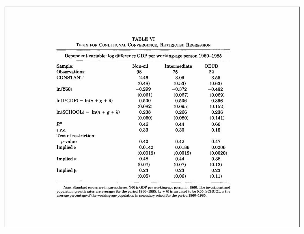
TABLE VI TESTS FOR CONDITIONAL CONVERGENCE, RESTRICTED REGRESSION
Dependent variable: log difference GDP per working-age person 1960-1985
Sample: Non-oil Intermediate OECD Observations: 98 75 22 CONSTANT 2.46 3.09 3.55
(0.48) (0.53) (0.63) ln(Y60) -0.299 -0.372 -0.402
(0.061) (0.067) (0.069) ln(I/GDP) - ln(n + g + 5) 0.500 0.506 0.396
(0.082) (0.095) (0.152) ln(SCHOOL) - ln(n + g + 5) 0.238 0.266 0.236
(0.060) (0.080) (0.141) R2 0.46 0.44 0.66 s.e.e. 0.33 0.30 0.15 Test of restriction:
p-value 0.40 0.42 0.47 ImpliedX 0.0142 0.0186 0.0206
(0.0019) (0.0019) (0.0020) Implied (x 0.48 0.44 0.38
(0.07) (0.07) (0.13) Implied 13 0.23 0.23 0.23
(0.05) (0.06) (0.11)
Note. Standard errors are in parentheses. Y60 is GDP per working-age person in 1960. The investment and population growth rates are averages for the period 1960-1985. (g + 5) is assumed to be 0.05. SCHOOL is the average percentage of the working-age population in secondary school for the period 1960-1985.
specifications that do not consider out-of-steady-state dynamics. Similarly, the greater importance of departures from steady state for the OECD would explain the finding of greater unconditional convergence. We find this interpretation plausible: World War II surely caused large departures from the steady state, and it surely had larger effects on the OECD than on the rest of the world. With a value of X of 0.02, almost half of the departure from steady state in 1945 would have remained by the end of our sample in 1985.
Overall, our interpretation of the evidence on convergence contrasts sharply with that of endogenous-growth advocates. In particular, we believe that the study of convergence does not show a failure of the Solow model. After controlling for those variables that the Solow model says determine the steady state, there is substantial convergence in income per capita. Moreover, conver- gence occurs at approximately the rate that the model predicts.
Estimation Results for Convergence Hypothesis
• Sum of coefficients on and in equation (16) should be equal in magnitude and opposite in sign to the coefficient on ln(n + g + δ).
• Cannot reject this restriction.
• Implied values for income share of physical capital of range from 0.38 to 0.48 and the implied values for income share of human capital is 0.23 in all three samples.
• These convergence regression estimates give larger weight to physical capital and a smaller weight to human capital compared to the estimates explaining variation in output per worker (Table II).
ln(sk ) ln(sh )